Real-Time RGBD Odometry for Fused-State Navigation Systems

Abstract

This article describes an algorithm that provides visual odometry estimates from sequential pairs of RGBD images. The key contribution of this article on RGBD odometry is that it provides both an odometry estimate and a covariance for the odometry parameters in real-time via a representative covariance matrix. Accurate, real-time parameter covariance is essential to effectively fuse odometry measurements into most navigation systems. To date, this topic has seen little treatment in research which limits the impact existing RGBD odometry approaches have for localization in these systems. Covariance estimates are obtained via a statistical perturbation approach motivated by real-world models of RGBD sensor measurement noise. Results discuss the accuracy of our RGBD odometry approach with respect to ground truth obtained from a motion capture system and characterizes the suitability of this approach for estimating the true RGBD odometry parameter uncertainty.

I Introduction

Visual image sensors, e.g., digital cameras, have become an important component to many autonomous and semi-autonomous navigational systems. In many of these contexts, image processing algorithms process sensed images to generate autonomous odometry estimates for the vehicle; referred to as visual odometry. Early work on visual odometry dates back more than 20 years and applications of this approach are pervasive in commercial, governmental and military navigation systems. Algorithms for visual odometry compute the change in pose, i.e., position and orientation, of the robot as a function of observed changes in sequential images. As such, visual odometry estimates allow vehicles to autonomously track their position for mapping, localization or both of these tasks simultaneously, i.e., the Simultaneous Localization and Mapping (SLAM) applications. The small form factor, low power consumption and powerful imaging capabilities of imaging sensors make them an attractive as a source of odometry in GPS-denied contexts and for ground-based, underground, indoor and near ground navigation.

While visual odometry using conventional digital cameras is a classical topic, recent introduction of commercial sensors that capture both color (RGB) images and depth (D) simultaneously, referred to as RGBD sensors, has created significant interest for their potential application for autonomous 3D mapping and odometry. These sensors capture color-attributed $(X,Y,Z)$ surface data at ranges up to 6m. from a 58.5H x 46.6V degree field of view. The angular resolution of the sensor is ~5 pixels per degree and sensed images are generated at rates up to 30 Hz.

As in other visual odometry approaches, RGBD-based odometry methods solve for the motion of the camera, referred to as ego-motion, using data from a time-sequence of sensed images. When the geometric relationship between the camera and vehicle body frame is known, estimated camera motions also serve as estimates for vehicle odometry.

Algorithms that compute odometry from RGBD images typically match corresponding 3D $(X,Y,Z)$ surface measurements obtained from sequential frames of sensed RGBD image data. Since the image data is measured with respect to the camera coordinate system, camera motions induce changes in the $(X,Y,Z)$ surface coordinates of stationary objects in the camera view. The transformation that aligns corresponding $(X,Y,Z)$ measurements in two frames indicates how the camera orientation and position changed between these frames which, as mentioned previously, also specifies vehicle odometry.

While several methods for RGBD odometry estimation exist in the literature, published work on this topic lacks sensitivity to the larger issue of integrating RGBD odometry estimates into autonomous navigation systems. Researchers and practitioners acknowledge that visual odometry can provide highly inaccurate odometry estimates; especially when incorrect correspondences are computed. As shown in Fig. 1, navigation systems cope with this issue by adding odometry sensors in the form of wheel-based odometry (ground vehicles) or Inertial Measurement Units (IMUs) (aerial vehicles) and subsequently fusing this data into a 3D state estimate for the vehicle. Fused state estimates are typically produced by filtering sensor data using an Extended Kalman Filter (EKF) [1] or particle filter. Regardless of the filter type, fused-state estimation requires uncertainty estimates for each sensor measurement that, for an EKF, re-weight the measurements by attributing values having low uncertainty larger weight than other values. As such, navigational systems that seek to leverage RGBD odometry require uncertainty estimates for these parameters.

For EKF-based navigation systems, absence of the RGBD odometry parameter covariance implies that these systems include hand-specified or ad-hoc estimates for the covariance of these parameters. For example, one potential approach in this context is to assume a worst-case covariance for the translational and orientation parameters via a user-specified constant-valued diagonal covariance matrix. Yet, without means for outlier rejection, artificially large covariances must be assumed to cope with the possibility of potentially inaccurate RGBD odometry parameters. When outlier rejection is applied, ad-hoc methods must be used that dynamically change the parameter covariances which artificially adjusts the weight of RGBD odometry estimates. While such ad-hoc approaches may be more effective in leveraging RGBD odometry values, the artificially chosen covariances do not characterize the true parameter uncertainty. As a result, even sophisticated ad-hoc methods will significantly limit the beneficial impact that RGBD odometry can have for system navigation.

The key contribution of this article on RGBD odometry is that it provides both an odometry estimate and a covariance for the odometry parameters in real-time via a representative covariance matrix. This article proposes a statistical perturbation-based approach based on observed RGBD measurement noise to compute the parameter covariance estimates essential for efficiently leveraging estimated RGBD odometry values in navigation systems. Results discuss the accuracy of our RGBD odometry approach with respect to ground truth obtained from a motion capture system and characterizes the suitability of this approach for estimating the true RGBD odometry parameter uncertainty.

This article is divided into six sections as follows: § II discusses prior work on RGBD odometry related to this article, § III discusses background information critical to the explanation of the odometry algorithm, § IV discusses the RGBD odometry and covariance parameter estimation algorithm, § V presents results for experimental odometry parameter and covariance estimation and performance of the odometry estimation algorithm versus ground truth data obtained via motion capture, § VI summarizes the impact of this work and discusses aspects of this work that motivate future research.

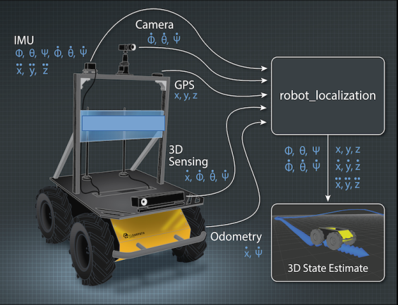
Figure 1: A typical fused-state estimator described in [1] is shown. Fused-state navigation systems integrate visual odometry, e.g., RGBD odometry, with odometry from sensors such as IMUs, GPS, and wheel odometry to provide a single 3D state estimate for the vehicle. Accurate fused-state estimation relies heavily on knowledge of uncertainty in each sensor measurement to determine the best possible state estimate. This article introduces an RGBD odometry algorithm that provides both odometry values and uncertainties for the estimated odometry values which are critical to this important application.

II Prior Work

Since the commercial introduction of RGBD sensors, researchers have been developing methods to leverage the additional depth data to improve state-of-the-art for navigation and mapping. We touch on the most popular approaches for RGBD odometry here which

In [2] authors compute odometry from RGBD images by expediting the ICP algorithm [3]. Their approach computes and matches edges from the RGB data in sequential frames to quickly find matching 3D points from the depth image. The depth images are then aligned by aligning 3D points at edge locations and uses the resulting transform as an initial guess to accelerate the convergence of the computationally-costly generalized ICP algorithm, [4], which solves for the final estimate using a point-to-plane error metric.

In [5] a MAV is navigated in dark environments using 6DoF localization provided by fusing a fast odometry algorithm and generalizing a ground-based Monte Carlo Localization approach [6] for their 6DoF MAV application. Real-time odometry is obtained by expressing the relative pose estimation problem as a differential equation on each 3D point that models the change in the 3D point location as a function of the changing pose parameters. The approach is made real-time by sub-sampling the image data which reduces the full-frame (640x480) image to a much smaller (80x60) image for processing.

In [7] a warping function is used to map pixels in sequential RGBD images. The warping function combines an appearance model with a depth/geometric model to solve for the transformation parameters that minimize the differences between measured RGB colors and depths in the warped/aligned RGBD images.

While each of the approaches above for RGBD odometry have different strengths and weaknesses, they all suffer from a lack of consideration of the parameter uncertainty. As mentioned in the introduction, no visual odometry approach has been demonstrated to be completely free of incorrect odometry estimates. As such, regardless of the sophistication and accuracy of the approach, it is critical to provide uncertainty measures for RGBD odometry estimates. Absence of this information severely limits the utility of this information for its primary purpose: as a component to a fused-state navigational system.

III Background Information

The proposed approach for odometry draws heavily from published results on RGBD sensor characterization, computer vision, image processing and 3D surface matching literature. This section includes aspects from the literature critical to understanding the RGBD odometry algorithm and subtle variations on published approaches we use that, to our knowledge, have not been previously published elsewhere.

III-A Robust Correspondence Computation in RGBD Image Pairs

Rather than matching all measured surface points and solving for the point cloud alignment using ICP [3] or GICP [4], our odometry reduces the measured data in both frames to a set of visually-distinct surface locations automatically selected via a user-specified OpenCV feature detection algorithm, e.g., SIFT [8], SURF [9] , BRIEF [10], ORB [11] etc. A user-specified OpenCV feature descriptor is then computed at each detection location to create a set of feature descriptors for each RGB image. Robust methods then compute a correspondence between the RGBD images in a two-stage process:

• Stage 1 identifies salient visual matches between the RGB feature descriptors using a symmetric version of Lowe’s ratio test.

• Stage 2 refines correspondences from Stage 1 by applying the Random Sample Consensus (RANSAC) algorithm [12] to identify the triplet of corresponding $(X,Y,Z)$ measurements that, when geometrically aligned, result in the largest amount of inliers, i.e., geometrically close, pairs in the remaining point set.

The two stages operate on distinct subsets measurements from the data. Stage 1 exploits salient measurements from the RGB image data. Stage 2 exploits salient measurements in the 3D data. While the order of the stages 1 and 2 could be switched, the computational cost of the RANSAC algorithm increases significantly when no initial correspondence is available (see [13] for RANSAC computational complexity analysis). This motivates use of RANSAC downstream from RGB feature matching which, for most OpenCV features, is significantly faster to compute.

Stage 1: Robust Image Feature Correspondence via Lowe’s Ratio Test and Symmetry Criteria

As with many time-based imaging and computer vision algorithms, e.g., optical flow, face tracking, and stereo reconstruction from images, our RGBD odometry approach seeks to find a collection of corresponding pixels from two sequential images in time. As in other approaches, we compute sets of visual features from each image, $(F,G)$, that are assumed invariant to small changes in viewpoint. Correspondences are found by pairing elements from the feature sets, $(f_{i},g_{j})$. These correspondences are found by imposing a metric on the feature space, e.g., a Euclidean metric $\left\|f_{i}-g_{j}\right\|$, and then associating features using a criterion on this metric, e.g., nearest neighbors: $j=\min_{k}\left(\left\|f_{i}-g_{k}\right\|,\,\,g_{k}\in G\right)$. Unfortunately, application of this type of matching often results in many incorrect correspondences; especially when many features share similar values.

In this work we adopt a symmetric version of Lowe’s ratio test [8] to identify and reject potentially incorrect visual feature correspondences. Conceptually, this is accomplished by examining the uncertainty in the match. If computation were not a concern, this uncertainty could be found by perturbing the value of $f_{i}$ and observing the variability of the corresponding element $g_{j}$ but this is not feasible in real-time applications. Lowe’s test simplifies this decision by dividing the distances between $f_{i}$ and it’s 2-nearest neighbors $(g_{j},g_{k})$ where $\left\|f_{i}-g_{j}\right\|\leq\left\|f_{i}-g_{k}\right\|$ creating the ratio $\frac{\left\|f_{i}-g_{j}\right\|}{\left\|f_{i}-g_{k}\right\|}$. A user-specified salience parameter, $\lambda_{ratio}$, is applied to reject correspondences that satisfy the inequality $\frac{\left\|f_{i}-g_{j}\right\|}{\left\|f_{i}-g_{k}\right\|}>\lambda_{ratio}$. Features that pass this test ensure the match for $f_{i}$ into the set of $G$ is salient since the two best candidate matches in $G$ have significantly different distances for their best and next-best matches. Unfortunately, Lowe’s ratio is asymmetric as it does not ensure that the match between $g_{j}$ into the set $F$ is also salient. Symmetry is achieved by applying the ratio test first for the element $f_{i}$; ensuring distinct matches from $f_{i}\rightarrow G$ and then again for $g_{j}$; ensuring distinct matches from $g_{j}\rightarrow F$. Feature matches that satisfy this symmetric version of Lowe’s ratio test are considered to be candidate correspondences between two images. Results shown in this article were generated by applying this test with $\lambda_{ratio}=0.8$ which ensures that, for each correspondence, the 2nd best match, $\left\|f_{i}-g_{k}\right\|$, has a distance that is 25% larger than the best match$\left\|f_{i}-g_{j}\right\|$.

Stage 2: Robust 3D $(X,Y,Z)$ Odometry via RANSAC and RANSAC Refinement

A second stage uses the image locations and depths of the visual correspondences from Stage 1 to generate a pair of $(X,Y,Z)$ point clouds. Since the correspondences between points in these clouds are given via the visual correspondence, it is possible to directly estimate the transformation in terms of a rotation matrix, $\mathbf{R}$, and translation, $\mathbf{t}$, that best-aligns the two pointsets in terms of the sum of their squared distances using solutions to the “absolute orientation” problem, e.g., [14, 15]. However, incorrect correspondences may still exist in the data and, if so, they can introduce significant error.

The RANSAC algorithm leverages the geometric structure of the measured 3D data to reject these incorrect correspondences. It accomplishes this by randomly selecting triplets of corresponding points, computing the transformation,$\left(\mathbf{R},\mathbf{t}\right)$, that best aligns the triangles these points describe and then scoring the triplet according to the number of observed inliers in the aligned point clouds. Inliers are determined by thresholding the geometric distance between corresponding points after alignment with a user-specified parameter, $\lambda_{inlier}$, such that a point pair $(\mathbf{p}_{i},\mathbf{p}_{j})$ is marked as an inlier if $\left\|\mathbf{p}_{i}-\left(\mathbf{R}\mathbf{p}_{j}+\mathbf{t}\right)\right\|<\lambda_{inlier}$. In this way, the RANSAC-estimated transformation, $\widehat{\left(\mathbf{R},\mathbf{t}\right)}$, is given by aligning the triplet of points having best geometric agreement (in terms of inlier count) between the two point clouds.

We use the RANSAC algorithm included as part of the Point Cloud Library (PCL v1.7) which also has an option to refine the inlier threshold. The refinement process allows the RANSAC algorithm to dynamically reduce the inlier threshold by replacing it with the observed standard deviation of the inlier distances at the end of each trial. Specifically the inlier threshold is replaced when the observed variation of the inliers is smaller than the existing distance threshold, e.g., for each refinement iteration the new threshold $\hat{\lambda}_{inlier}=\min\left(3\sigma_{inliers},\lambda_{inlier}\right)$. Results shown in this article are generated using PCL’s RANSAC algorithm (with refinement) with user-specified settings that allow a maximum of 200 RANSAC iterations and an inlier distance threshold of $\lambda_{inlier}=5cm.$

III-B RGBD Cameras: Calibration, 3D Reconstruction, and Noise

Calibration

Primesense sensors are shipped with factory-set calibration parameters written into their firmware. These parameters characterize the physical characteristics of the RGB and IR/Depth cameras that make up the RGBD sensor and allows data from these cameras to be fused to generate color-attributed $(X,Y,Z)$ point clouds. While it is possible to use the factory-provided calibration settings, better odometry estimates are possible using experimentally calibrated parameters. Calibration describes the process of estimating the in-situ image formation parameters for both the RGB and IR imaging sensors and the transformation, i.e., rotation and translation, between these two sensors. Calibration of the intrinsic, i.e., image formation, parameters for each camera, provide values for the $(x,y)$ focal distance,$(f_{x},f_{y})$, the image center/principal point, $(c_{x},c_{y}),$ and the $(x,y)$ pixel position shift, $(\delta_{x},\delta_{y})$, that occur due to radial and tangential lens distortions. Estimates for these values are obtained by detecting (via image processing) the $(x,y)$ image positions of features in images of a calibration pattern having a-priori known structure (typically a chess board). After intrinsic calibration, the extrinsic parameters of the sensor pair, i.e, the relative position and orientation of the RGB and IR sensor, is estimated by applying a similar procedure to images from both cameras when viewing the same calibration pattern.

The key benefit of accurate calibration is to reduce the uncertainty in the location of projected depth and color measurements (intrinsic parameters) and to align/register the depth and color measurements from these two sensors to a common $(x,y)$ image coordinate system (extrinsic parameters) which, for simplicity, is taken to coincide with the coordinate system of the RGB camera sensor. When using the factory-shipped calibration values, this registration can occur on-board the Primesense sensor (hardware registration). Experimentally estimated calibration parameters are typically more accurate than factory settings at the expense of additional computational cost (software registration).

Work in this article uses the factory-provided extrinsic calibration values for hardware registration of the RGB/IR images and experimentally calibrated values for the intrinsic/image formation parameters. This compromise uses RGBD sensor hardware to perform the computationally costly registration step and software to reconstruct 3D position values. While use of the factory-provided extrinsic parameters can potentially sacrifice accuracy, we found these values resulted in similar odometry and simultaneously significantly reduced the software driver execution overhead. As RGBD cameras are fixed focal length, the camera calibration parameters are fixed in time and are recalled by the odometry algorithm during initialization.

Point Cloud Reconstruction

Measured 3D $(X,Y,Z)$ positions of sensed surfaces can be directly computed from the intrinsic RGBD camera parameters and the measured depth image values. The $Z$ coordinate is directly taken as the depth value and the $(X,Y)$ coordinates are computed using the pinhole camera model. In a typical pinhole camera model 3D $(X,Y,Z)$ points are projected to $(x,y)$ image locations, e.g., for the image columns the $x$ image coordinate is $x=f_{x}\frac{X}{Z}+c_{x}-\delta_{x}$. However, for a depth image, this equation is re-organized to “back-project” the depth into the 3D scene and recover the 3D $(X,Y)$ coordinates as shown by equation (1)

$$\begin{array}[]{ccc}X&=&(x+\delta_{x}-c_{x})Z/f_{x}\\ Y&=&(y+\delta_{y}-c_{y})Z/f_{y}\\ Z&=&Z\end{array}$$ (1)

where $Z$ denotes the sensed depth at image position $(x,y)$ and the remaining values are the intrinsic calibration parameters for the RGB camera.

Measurement Noise

Studies of accuracy for the Kinect sensor show that assuming a Gaussian noise model for the normalized disparity provides good fits to observed measurement errors on planar targets where the distribution parameters are mean $0$ and standard deviation $\sigma_{d^{\prime}}=0.5$ pixels [16]. Since depth is a linear function of disparity, this directly implies a Gaussian noise model having mean $0$ and standard deviation $\sigma_{Z}=\frac{m}{f_{x}b}Z^{2}\sigma_{d^{\prime}}$ for depth measurements where $\frac{m}{f_{x}b}=-2.85e^{-3}$ is the linearized slope for the normalized disparity empirically found in [16]. Since 3D $(X,Y)$ coordinates are also derived from the pixel location and the depth, their distributions are also known as shown below:

$$\begin{array}[]{ccc}\sigma_{X}&=&\frac{x_{im}-c_{x}+\delta_{x}}{f_{x}}\sigma_{Z}=\frac{x_{im}-c_{x}+\delta_{x}}{f_{x}}(1.425e^{-3})Z^{2}\\ \sigma_{Y}&=&\frac{y_{im}-c_{y}+\delta_{y}}{f_{y}}\sigma_{Z}=\frac{y_{im}-c_{y}+\delta_{y}}{f_{y}}(1.425e^{-3})Z^{2}\\ \sigma_{Z}&=&\frac{m}{f_{x}b}Z^{2}\sigma_{d^{\prime}}=(1.425e^{-3})Z^{2}\end{array}$$ (2)

These equations indicate that 3D coordinate measurement uncertainty increases as a quadratic function of the depth for all 3 coordinate values. However, the quadratic coefficient for the $(X,Y)$ coordinate standard deviation is at most half that in the depth direction, i.e., $(\sigma_{X},\sigma_{Y})\approx 0.5\sigma_{Z}$ at the image periphery where $\frac{x-c_{x}}{f}\approx 0.5$, and this value is significantly smaller for pixels close to the optical axis.

For example, consider a “standard” Primesense sensor having no lens distortion and typical factory-set sensor values: $(f_{x},f_{y})=f=586\pm 30$ for focal length, $(640,480)$ for image $(x,y)$ dimension, and $(c_{x},c_{y})=(320,240)$ for the image center. In this case the ratios $(\frac{x-c_{x}+\delta_{x}}{f_{x}},\frac{y-c_{y}+\delta_{y}}{f_{y}})=(0,0)$ at the image center and $(\frac{x-c_{x}+\delta_{x}}{f_{x}},\frac{y-c_{y}+\delta_{y}}{f_{y}})=(0.548\pm 0.028,.411\pm 0.021)$ at the $(x,y)$ positions on the image boundary. With this in mind, the $(X,Y,Z)$ coordinates of a depth image are modeled as measurements from a non-stationary Gaussian process whose mean is $0$ at all points but whose variance changes based on the value of the triplet $(x,y,Z)$.

III-C Odometry Covariance Estimation

The RGBD reconstruction equations (1) and measurement noise equations (2) provide a statistical model for $(X,Y,Z)$ measurement errors one can expect to observe in RGBD data. Our approach for odometry parameter covariance estimation creates two point clouds from the set of inliers identified by the previously mentioned RANSAC algorithm. We then simulate an alternate instance of the measured point cloud pair by perturbing the $(X,Y,Z)$ position of each point with random samples taken from a $0$ mean Gaussian distribution whose standard deviation is given by measurement noise equations (2). Each pair of perturbed point clouds is aligned via the solution to the absolute orientation problem ([14]) to generate an estimate of the odometry parameters. For a set of $N$ perturbed point cloud pairs, let $\xi_{n}$ denote the odometry parameters obtained by aligning the $n^{th}$ simulated point cloud pair. Unbiased estimates for the statistical mean, $\widehat{\mu}$, and covariance, $\widehat{\Sigma}$, of the odometry parameters is computed via:

$$\widehat{\mu}=\frac{1}{N}\sum_{n=1}^{N}\xi_{n},\,\,\,\,\widehat{\sum}=\frac{1}{N-1}\sum_{n=1}^{N}(\xi_{n}-\widehat{\mu})(\xi_{n}-\widehat{\mu})^{t}$$

Covariance estimates published in this article are generated by perturbing each point cloud pair 100 times, i.e., $N=100$.

IV Methodology

Our approach for odometry seeks to compute instantaneous odometry directly from sensor measurements in a manner similar to a sensor driver. As such, there is no attempt for higher-level processing such as temporal consistency [17] or keyframing [18]. Given this design goal, such tasks are more appropriate for user-space or client-level application development where the problem domain will drive the algorithm choice and design.

The following steps outline of the RGBD odometry driver:

1. Reduce the dimension of the data by converting the RGB image into a sparse collection of feature descriptors that characterize salient pixels in the RGB image.

   1. Discard measurements at the image periphery and measurements having invalid or out-of-range depth values.

   2. Detect feature locations in the RGB image and extract image descriptors for each feature location.

2. For sequential pairs of RGBD images in time, match their feature descriptors to compute candidate pixel correspondences between the image pair using Lowe’s Ratio test as discussed in § III.

3. Using only the candidate pixel correspondences from (2), compute two sparse $(X,Y,Z)$ point clouds from the RGBD feature correspondences using equation (1) from § III.

4. Apply Random Sample Consensus (RANSAC) to find the triplet of corresponding $(X,Y,Z)$ points that, when aligned using the rotation and translation $\widehat{\left(\mathbf{R},\mathbf{t}\right)}$, maximize the geometric agreement (number of inliers) of the corresponding point cloud data as described in § III.

5. The subset of points marked as inliers from (4) are used to generate a new pair of point clouds. We then perturb the $(X,Y,Z)$ data in each point cloud according to the measurement noise models of equation (2) and empirically compute the 6x6 covariance matrix, $\widehat{\sum}$, of the odometry parameters as described in § III.

The 6DoF odometry estimate, $\xi$, is taken taken directly from the alignment transformation parameters, $\widehat{\left(\mathbf{R},\mathbf{t}\right)}$, computed in step 4. These values characterize the vehicle position and angular velocities during the time interval spanned by each measured image pair. Step 5 provides, $\widehat{\Sigma}$, our estimate for the covariance of the odometry parameters.

V Results

To evaluate our approach for RGBD odometry we implemented the algorithm as a C++ node using the Robot Operating System (ROS) development framework [19]. Experiments were conducted using an XTion Pro Live RGBD camera at full-frame (640x480) resolution and framerate (30Hz). The frame-to-frame odometry performance is tracked by calibrating the pose of the RGBD camera to a motion capture system (Optitrack). In our experiments, we initialize the RGBD camera pose to coincide with the measured pose as given by averaging 5 seconds (500 samples) of motion capture data while the RGBD camera is stationary. After initialization, the pose of the RGBD camera is measured by the motion capture systems independent from the pose obtained via the time integration of the frame-to-frame odometry estimates.

Name	Value
OpenCV Detector Algorithm	“ORB”
OpenCV Descriptor Algorithm	“ORB”
$\lambda_{ratio}$	0.8
$\lambda_{inlier}$	5cm.
RANSAC MAX ITERATIONS	200
NUMBER PERTURBATIONS	100

Table I: Parameters used for the proposed RGBD odometry algorithm to generate results in this article.

Using the algorithm parameter values shown in Table I, our RGBD algorithm runs in real-time (30Hz) on full-frame RGBD data on a quad-core Intel i5 CPU with a clock speed 2.67GHz and our results are generated using this configuration and hardware. We have also run this algorithm, without modification, on an Odroid-XU3 which is a very small (9.4cm.x7cm.x1.8cm.) and lightweight (~ 72gram) single board computer having a quad-core Arm7 CPU with a clock speed of 1.4GHz. Our RGBD algorithm runs on full-frame RGBD data at a rate of 7.25Hz on this platform and has similar odometry performance.

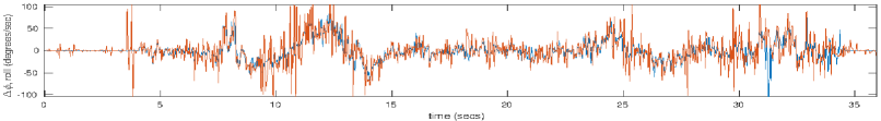
(a)

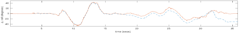
(b)

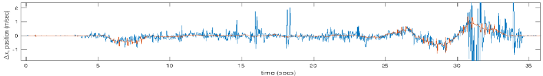
(c)

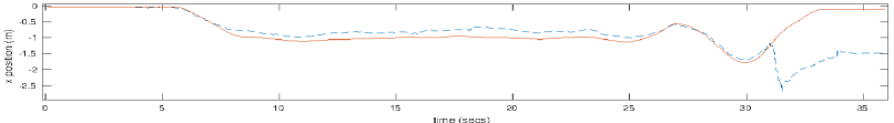
(d)

Figure 2: (a,b,c,d) show estimated (blue/dashed) and motion-capture (orange/solid) values for the velocity and position of the body-frame $x$-axis during the experiment. (a,b) show the $x$-axis angular velocity and angular position (roll) respectively. (c,d) show x position velocities and the absolute x position respectively. As one would expect, pairs (a,b) and (c,d) have (integral,derivative) relationships. Inaccurate velocities from visual odometry, e.g., those at time 32 sec., are coupled with large covariance (see Fig. 3 time index 32 sec.) which indicates to fused-state navigation systems that these estimates are not reliable.

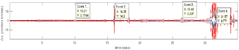
(a)

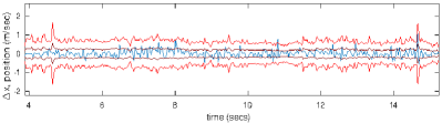
(b)

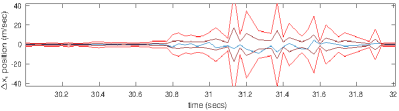
(c)

Figure 3: Plots (a-c) show three views of odometry error (blue) and the $\pm 1\sigma$ (purple) and $\pm 3\sigma$ (red) confidence intervals for the $x$ position velocity during the 35 second odometry experiment. (b,c) show close-up views of time intervals (4,14) sec., (b), and, (30,32) sec. showing instances having normal odometry, (b), and highly uncertain odometry, (c). Four time events of interest are marked on plot (a). Events 1 and 3 mark instances where odometry is tracking well and parameter variance is smoothly changing. Events 2 and 4 mark instances where the odometry is perceived to be highly-uncertain and have large associated covariance estimates. As evident in these plots, covariance values dramatically increase for inaccurate odometry estimates. This allows fused-state navigation to ignore unreliable odometry estimates when they occur.

Our results analyze a single 35 second experiment with motion-tracked RGBD odometry to assess algorithm performance. In this experiment the sensor views an indoor environment (the laboratory) which includes office furniture, boxes, chairs and a camera calibration pattern. The full 6DoF range of motions were generated in the experiment by manually carrying the camera around the laboratory and includes motions having simultaneous $(X,Y,Z)$ and (roll, pitch, yaw) variations at positional velocities approaching 1m/s and angular velocities approaching 50-100 degrees/s. The experiment also includes medium (~2m. range) and long (~5m. range) depth images and images of highly distinct surfaces, e.g., shipping boxes and textured floor tiles as well as visually confusing surfaces, e.g., a calibration pattern consisting of regularly spaced black squares on a white background. All of these contexts promise to provide opportunities to observe and characterize the odometry parameter estimate accuracy and the accuracy of the associated covariance of these parameters.

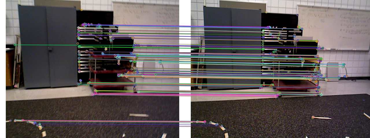
(a) Event 1: Accurate odometry: depth ~3m., slow velocity (no blurring).

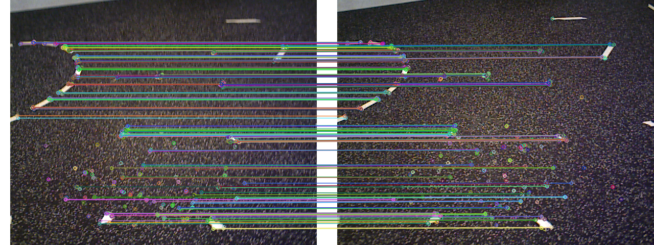
(b) Event 2: Odometry error: depth ~1m., some incorrect visual correspondences.

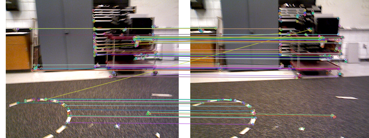
(c) Event 3: Accurate odometry: depth ~3m., higher velocity (blurring).

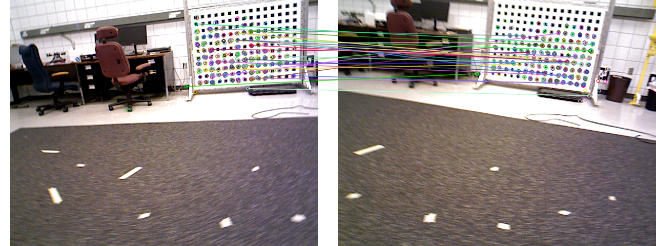
(d) Event 4: Worst-case scenario: high velocity, incorrect visual correspondences.

Figure 4: (a-d) show RGB image pairs from the RGBD sensor at Events 1-4 from Fig. 3 respectively. (Left column) Events (1) and (3) show that correct visual correspondences lead to accurate RGBD odometry. In these cases the estimated odometry covariance tends to vary smoothly and increases roughly proportional to vehicle velocity which induces blur to images. (Right column) Events (2) and (4) show that incorrect visual correspondences lead to inaccurate RGBD odometry. While this can introduce error to RGBD-only based estimates for pose (Fig. 2(b,d)), the estimated covariance at these time instances increases dramatically (see red curve of Fig. 3). This allows fused-state navigation systems to automatically reject these estimates when they occur. As such, the covariance estimation approach proposed here enables fused-state navigation systems to benefit from accurate RGBD odometry when it is available.

Figure 2 depicts estimated (blue/dashed) and motion-capture (orange/solid) values for the velocity and position of the of the body-frame x-axis during the experiment. Since motion capture systems measure absolute pose, i.e., position and orientation, velocities must be computed by taking the time-differential of the motion capture data. For this reason, the motion capture angular velocities are particularly noisy since perturbations in the measured orientation over short time intervals induce large instantaneous angular velocity measurements. The close proximity of the estimated and measured velocities in plots (a,c) show that, in most cases, the RGBD odometry algorithm tracks well. Errors in angular velocity visible in (a) are localized to time instants at time indices 16 sec. and 32 sec. The error at time 16 sec. appears to be due to a combination of a erroneously high velocity estimate from the motion capture and erroneously low error from the estimated odometry. The error at time 32 sec. occurs when the camera makes inaccurate visual matches that cannot be corrected and result in a failed (highly inaccurate) odometry estimate. A similar pattern exists for the $x$ position, (d), and position velocities, (c). As one would expect, odometry errors in (a,c) introduce offsets between the motion capture and estimated body frame $x$-axis angle (b) and $x$ position (d) since these quantities are obtained by integrating the their respective velocity signals (a,c).

Figure 3 depicts odometry errors for the vehicle, i.e., body-frame, $x$-axis (blue) and the estimated $\pm 1\sigma$ (purple) and $\pm 3\sigma$ (red) confidence intervals for the $x$-axis velocity parameter. Four events of interest are marked in Fig. 3. Events (1,3) demonstrate typical, i.e., nominal, RGBD odometry performance as the vehicle velocity and scene depth simultaneously vary. Events (2,4) demonstrate atypical, i.e., potentially erroneous, RGBD odometry and demonstrate that, for both time instances where the odometry is inaccurate, the covariance dramatically increases.

Analysis of the odometry error indicates that the estimated covariances underestimate the experimentally measured odometry parameter uncertainty. This is to be expected since the simulated point clouds from which this covariance is derived does not account for noise from many sources such as incorrect visual feature correspondences. Despite this, the estimated covariances increase and decrease in a manner that is approximately proportional to the experimentally observed parameter covariance.

Analysis of the data collected shows that taking $\Sigma=9\widehat{\Sigma}$ will place ~99% of measurements within their respective $3\sigma$ bounds for all 6DoF. While the error distributions are not Gaussian, they behave reasonably well and $\Sigma$ should be a functional measure for sensor fusion. For this reason, we propose taking $\Sigma=9\widehat{\Sigma}$ as an estimate for the measurement uncertainty (Further analysis of the required multiple to place ~95% of sample within $2\sigma$ may be a more practical choice.)

Figure 3 shows the associated $\pm 3\sigma$ curves for x position velocity estimates (red). Inspection of the covariance curve shows smooth variations where the odometry parameters are valid that tend to increase with vehicle velocity. The curve also includes large jumps in the covariance, e.g., Events (2,4), where potentially invalid odometry estimates occur.

Figure 3(a-c) depicts representative image pairs for Events 1-4 respectively. In each case, the image pair is shown with 2D visual features indicated by circles on the image. The subset of visual features that have been matched, as described in Step (2) of our algorithm (see § IV), have a line shown that connects corresponding feature locations in the image pair. The left column shows frame pairs from approximately time index 10 sec. and 26 sec. At these times the RGBD camera views similar scenes but has significantly different velocities. The velocity increase is visually apparent in the blurring artifacts which are absent in Event 1 and present in Event 3. We feel that image blur due to higher vehicle velocity contributes to inexact visual feature matches and that the observed increase in parameter covariance that coincides in time with higher vehicle velocities is evidence of this phenomena. Events (2,4) show instances where we have either intentionally (Event 4) or unintentionally (Event 2) caused the visual odometry estimate to fail. The potential for failure in visual odometry is a phenomenon shared in differing degrees by all visual odometry algorithms. In this article, one can see that the RGBD odometry parameter covariance increases dramatically in these contexts which allows fused-state navigational systems to autonomously discard these estimates when they do occur.

VI Conclusion

This article proposes a method to estimate 6DoF odometry parameters and their parameter covariance from RGBD image data in real-time. The proposed method applies robust methods to accurately identify pairs of $(X,Y,Z)$ surface measurements in sequential pairs of images. Using RGBD sensor $(X,Y,Z)$ measurement and measurement noise models, perturbations are introduced to corresponding pairs of $(X,Y,Z)$ points to simulate plausible alternative odometry estimates for the same image pair. The covariance of the resulting odometry parameters serves as an estimate for odometry parameter uncertainty in the form of a full-rank 6x6 covariance matrix. Observation of the odometry errors with respect to a calibrated motion capture system indicate that the estimated covariances underestimate the true uncertainty of the odometry parameters. This is to be expected since the perturbation approach applied does not model all sources of uncertainty in the estimate. While many additional error sources exist, we feel that modeling uncertainty in correspondences and, to a lesser degree, uncertainty in the true $(x,y)$ projected pixel position, i.e., $(\delta_{x},\delta_{y})$ from equations (1) show the most promise for explaining differences observed between the apparent experimental parameter covariance and our real-time estimate for that value. Despite this, real-time covariances estimated by the proposed algorithm increase and decrease in a manner that is approximately proportional to the experimentally observed parameter covariance. As such, we propose pre-multiplying estimated covariances by an experimentally motivated factor ($9\widehat{\Sigma}$). The resulting odometry is real-time, representative of the true uncertainty and modestly conservative which makes it ideal for inclusion in typical fused-state odometry estimation approaches. This dynamic behavior greatly expands the navigational benefits of RGBD sensors by leveraging good RGBD odometry parameter estimates when they are available and vice-versa. This is especially important in situations where a pairwise RGBD odometry fails to return a plausible motion as evidenced in our experiments which show a dramatic increases in parameter covariance for these events.

VII Acknowledgment

This research is sponsored by an AFRL/National Research Council fellowship and results are made possible by resources made available from AFRL’s Autonomous Vehicles Laboratory at the University of Florida Research Engineering Education Facility (REEF) in Shalimar, FL.

References

- [1] T. Moore and D. Stouch, “A generalized extended kalman filter implementation for the robot operating system,” in Proceedings of the 13th International Conference on Intelligent Autonomous Systems (IAS-13), Springer, July 2014.
- [2] I. Dryanovski, C. Jaramillo, and J. Xiao, “Incremental registration of rgb-d images,” in Robotics and Automation (ICRA), 2012 IEEE International Conference on, pp. 1685–1690, May 2012.
- [3] P. Besl and N. D. McKay, “A method for registration of 3-d shapes,” Pattern Analysis and Machine Intelligence, IEEE Transactions on, vol. 14, pp. 239–256, Feb 1992.
- [4] A. Segal, D. Haehnel, and S. Thrun, “Generalized-ICp,” in Proceedings of Robotics: Science and Systems, (Seattle, USA), June 2009.
- [5] Z. Fang and S. Scherer, “Real-time onboard 6dof localization of an indoor mav in degraded visual environments using a rgb-d camera,” in Robotics and Automation (ICRA), 2015 IEEE International Conference on, pp. 5253–5259, May 2015.
- [6] S. Thrun, W. Burgard, and D. Fox, Probabilistic Robotics (Intelligent Robotics and Autonomous Agents). The MIT Press, 2005.
- [7] C. Kerl, J. Sturm, and D. Cremers, “Dense visual SLAM for rgb-d cameras,” in Intelligent Robots and Systems (IROS), 2013 IEEE/RSJ International Conference on, pp. 2100–2106, Nov. 2013.
- [8] D. G. Lowe, “Distinctive image features from scale-invariant keypoints,” Int. J. Comput. Vision, vol. 60, pp. 91–110, Nov. 2004.
- [9] H. Bay, A. Ess, T. Tuytelaars, and L. Van Gool, “Speeded-up robust features (surf),” Comput. Vis. Image Underst., vol. 110, pp. 346–359, June 2008.
- [10] M. Calonder, V. Lepetit, C. Strecha, and P. Fua, “Brief: Binary robust independent elementary features,” in Proceedings of the 11th European Conference on Computer Vision: Part IV, ECCV’10, (Berlin, Heidelberg), pp. 778–792, Springer-Verlag, 2010.
- [11] E. Rublee, V. Rabaud, K. Konolige, and G. Bradski, “Orb: An efficient alternative to sift or surf,” in Proceedings of the 2011 International Conference on Computer Vision, ICCV ’11, (Washington, DC, USA), pp. 2564–2571, IEEE Computer Society, 2011.
- [12] M. A. Fischler and R. C. Bolles, “Random sample consensus: A paradigm for model fitting with applications to image analysis and automated cartography,” Commun. ACM, vol. 24, pp. 381–395, June 1981.
- [13] R. Schnabel, R. Wahl, and R. Klein, “Efficient ransac for point-cloud shape detection,” Computer Graphics Forum, vol. 26, pp. 214–226, June 2007.
- [14] S. Umeyama, “Least-squares estimation of transformation parameters between two point patterns,” IEEE Trans. Pattern Anal. Mach. Intell., vol. 13, pp. 376–380, Apr. 1991.
- [15] B. K. P. Horn, “Closed-form solution of absolute orientation using unit quaternions,” Journal of the Optical Society of America A, vol. 4, no. 4, pp. 629–642, 1987.
- [16] K. Khoshelham and S. O. Elberink, “Accuracy and resolution of kinect depth data for indoor mapping applications,” Sensors, vol. 12, no. 2, p. 1437, 2012.
- [17] L. De-Maeztu, U. Elordi, M. Nieto, J. Barandiaran, and O. Otaegui, “A temporally consistent grid-based visual odometry framework for multi-core architectures,” J. Real-Time Image Process., vol. 10, pp. 759–769, Dec. 2015.
- [18] S. Leutenegger, S. Lynen, M. Bosse, R. Siegwart, and P. Furgale, “Keyframe-based visual-inertial odometry using nonlinear optimization,” Int. J. Rob. Res., vol. 34, pp. 314–334, Mar. 2015.
- [19] M. Quigley, K. Conley, B. P. Gerkey, J. Faust, T. Foote, J. Leibs, R. Wheeler, and A. Y. Ng, “Ros: an open-source robot operating system,” in ICRA Workshop on Open Source Software, 2009.