Symmetry Breaking in Symmetric
Tensor Decomposition

Abstract.

In this note, we consider the highly nonconvex optimization problem associated with computing the rank decomposition of symmetric tensors. We formulate the invariance properties of the loss function and show that critical points detected by standard gradient based methods are symmetry breaking with respect to the target tensor. The phenomena, seen for different choices of target tensors and norms, make possible the use of recently developed analytic and algebraic tools for studying nonconvex optimization landscapes exhibiting symmetry breaking phenomena of similar nature.

1. Introduction

We consider the problem of approximating a symmetric tensor as a sum of rank-1 symmetric tensors. Concretely, given an order $n$ symmetric tensor $T\in{\rm Sym}^{n}(\mathbb{R}^{d})$ and rank $k\in\mathbb{N}$, we study the nonconvex optimization problem

$$\min_{W\in M(k,d)}{\mathcal{L}}_{\star}(W)\coloneqq\left\|\sum_{i=1}^{k}\mathbf{w}_{i}^{\otimes{}n}-T\right\|_{\star}^{2},$$ (1)

with $M(k,d)$ denoting the space of $k\times d$ matrices, $\|\cdot\|_{\star}$ a tensor norm, and $\mathbf{w}_{i}$ the $i$-th row of $W$. We emphasize odd $n$ where (1) is equivalent to standard tensor rank decomposition, also known as the real symmetric canonical polyadic decomposition (CPD). However, methods are quite general.

The problem of finding a tensor approximation of bounded rank arises naturally in various scientific fields, including machine learning, biomedical engineering and psychometrics, see [1, 2, 3, 4, 5, 6, 7] and references therein for applications. The associated optimization problem is highly nonconvex and exhibits a variety of saddles and spurious (i.e., non-global local) minima that can cause a complete failure of gradient-based optimization methods. It is therefore of interest to study and characterize geometric obstructions of the this nature that exist in the associated loss landscape.

In this note, we show that, empirically, critical points of ${\mathcal{L}}_{\star}$ are symmetry breaking, a property defined in terms of isotropy groups, i.e., the group of all row and column permutations, denoted by $(S_{k}\times S_{d})_{C}\subseteq S_{k}\times S_{d}$, that fix the weights of a given critical point $C\in M(k,d)$. We found that critical points detected by gradient-based methods $(S_{k}\times S_{d})_{C}$ are typically large and conform with the structure of the target tensor $T$ (and so lie on low-dimensional subspaces), see Figure 1. The presence of symmetry breaking phenomena makes possible the derivation of sharp analytic estimates for families of critical points, their loss and their Hessian spectrum [8].

Our contributions in order of appearance may be stated as follows. In Section 3, invariance properties of ${\mathcal{L}}_{\star}$ are studied for different choices of inner products and target tensors, emphasizing the dependence of the invariance properties on the target tensor. In Section 4, numerical results are provided, indicating various isotropy groups of critical points that are found numerically. Results are given for the Frobenius inner product of order 3 and order 5 tensors, and for the inner product associated with the standard Gaussian distribution. Relevant background from multilinear algebra and group action is briefly reviewed in Section 2.

Next, we relate our results to the existing literature.

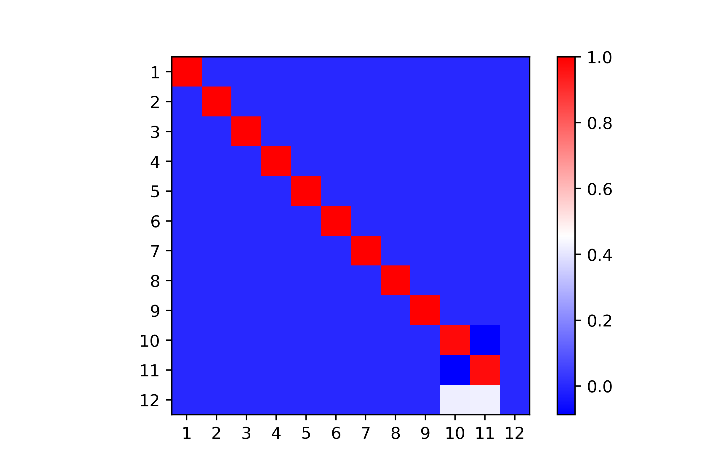
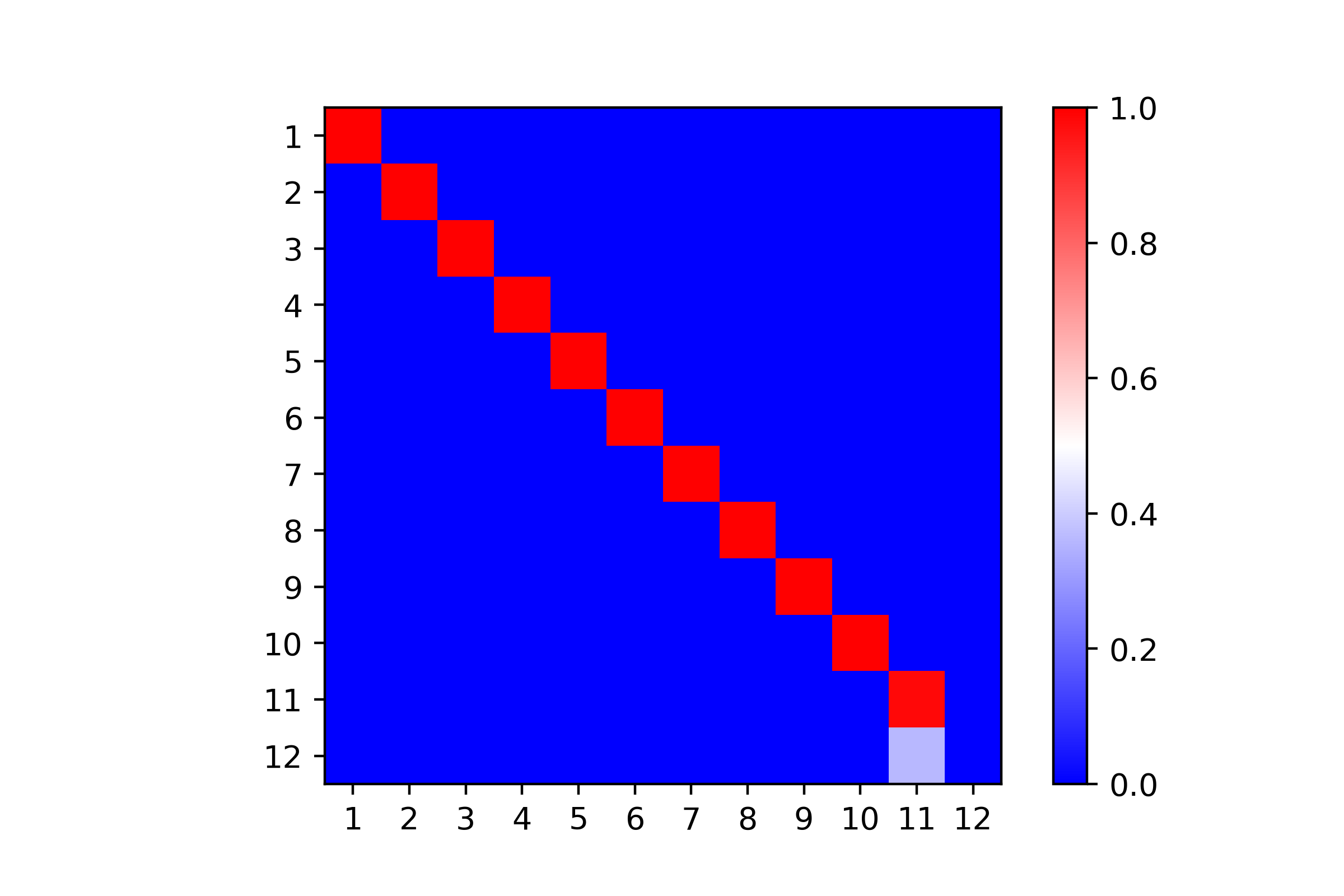
Figure 1. Spurious minima of optimization problem (1) under the Frobenius norm and problem parameters $d=k=12$, order $3$ symmetric tensors and target tensor $T=\sum_{i=1}^{k}\mathbf{e}_{i}^{\otimes{}3}$. (Left) a $12\times 12$-spurious minimum fixed by the group of row and column permutations $\Delta(S_{9}\times S_{2}\times S_{1})\subseteq S_{12}\times S_{12}$. (Right) a $12\times 12$-spurious minimum fixed by $\Delta(S_{10}\times S_{1}\times S_{1})$.

Symmetric tensor decomposition.

We briefly mention current algorithms for symmetric tensor decomposition. A straightforward yet practical method is based on direct first-order optimization of $\mathcal{L}$ in (1); see [9] and the Matlab implementations [10, 11]. A more computationally intensive although provable method (assuming $T$ is rank $r$ and $r=O(n^{\frac{d-1}{2}})$) was provided in [12], based on an algebraic construction called generating polynomials. For $n=3$ and $r\leq d$, a classic but theoretically convenient method was derived from simultaneous diagonalization of matrix slices [13] . For $n=4$ and $r=O(n^{2})$, the work [14] presented a provable algorithm using matrix eigendecompositions, which was robustified using ideas from the sums-of-squares hierarchy in [15]. In [16], a tensor power method was used, constructed from a matrix flattening of $T$, to find the components $\mathbf{w}_{i}$ sequentially. Also, [17] showed how to implement direct optimization of (1) in an efficient manner for moment tensors $T$ in an online setting.

Symmetry breaking in nonconvex loss landscapes.

It has been recently found that spurious minima occurring for a version of optimization problem (1) defined by use of the ReLU activation break the symmetry of global minima [18] (a formal exposition shall be given later in Section 3). Here, we report phenomena of symmetry breaking occurring for symmetric tensor decomposition problems. These were later used in [19] to study families of critical points building on methods developed in a line of work concerning phenomena of symmetry breaking, which we now survey. In [20], path-based techniques are introduced, allowing the construction of infinite families of critical points for ReLU two-layer networks using Puiseux series. In [21], results from the representation theory of the symmetric group are used to obtain precise analytic estimates on the Hessian spectrum. In [22], it is shown that certain families of saddles transform into spurious minima at a fractional dimensionality. In addition, Hessian spectra at spurious minima are shown to coincide with that of global minima modulo $O(d^{-{1}/{2}})$-terms. In [23], it is proved that adding neurons can turn symmetric spurious minima into saddles. In [24], generic $S_{d}$-equivariant steady-state bifurcation is studied, emphasizing irreducible representations along which spurious minima may be created and annihilated. In [25], it is shown that the way subspaces invariant to the action of subgroups of $S_{d}$ are arranged relative to ones fixed by the action determines the admissible types of structure and symmetry of curves along which ${\mathcal{L}}$ is minimized and maximized.

2. Preliminaries

We review relevant background material from multilinear algebra and group actions needed for a formal study of symmetry breaking.

2.1. Tensor preliminaries

A tensor of order $n$ is an element of the tensor product of $n$ vector spaces $V_{1}\otimes\ldots\otimes V_{n}$. Assuming $V_{i}$ are real vector spaces, we may choose a base for each factor $V_{i}$ and so identify a tensor with a multi-dimensional array in $\mathbb{R}^{d_{1}\times\ldots\times d_{n}}$ with $d_{i}=\dim(V_{i})$. We write $T_{i_{1},\ldots,i_{n}}$ for the $(i_{1},\ldots,i_{n})$-th coordinate of $T$. Given vectors $\mathbf{v}_{i}\in\mathbb{R}^{d_{i}}$, $i=1,\ldots,n$, we write $\mathbf{v}_{1}\otimes\ldots\otimes\mathbf{v}_{n}$ for the outer product of these vectors, that is, the element in $\mathbb{R}^{d_{1}}\otimes\ldots\otimes\mathbb{R}^{d_{n}}$ such that $(\mathbf{v}_{1}\otimes\ldots\otimes\mathbf{v}_{n})_{i_{1},\ldots,i_{n}}=({v_{1}})_{i_{1}}\ldots(v_{n})_{i_{n}}$. Also, we write $\mathbf{v}^{\otimes n}:=\mathbf{v}\otimes\ldots\otimes\mathbf{v}$ ($n$-times). The Frobenius inner product of two tensors $T,S$ of the same shape is defined to be $\langle T,S\rangle_{F}=\sum_{i_{1},\ldots,i_{n}}T_{i_{1}\ldots i_{n}}S_{i_{1}\ldots i_{n}}$. We will also consider other inner products of tensors. For the Frobenius inner product,

$$\langle\mathbf{v}_{1}\otimes\ldots\otimes\mathbf{v}_{n},\mathbf{w}_{1}\otimes\ldots\otimes\mathbf{w}_{n}\rangle_{F}=\prod_{i=1}^{n}\langle\mathbf{v}_{i},\mathbf{w}_{i}\rangle$$ (2)

for all $\mathbf{v}_{i},\mathbf{w}_{i}\in\mathbb{R}^{d_{i}},i=1,\ldots,n$. In particular, $\langle\mathbf{v}^{\otimes n},\mathbf{w}^{\otimes n}\rangle_{F}=\langle\mathbf{v},\mathbf{w}\rangle^{n}$.

A tensor $T\in(\mathbb{R}^{d})^{\otimes{}n}$ is symmetric if it is invariant under permutation of indices, that is, if $T_{i_{1},\ldots,i_{n}}=T_{i_{\sigma(1)},\ldots,i_{\sigma(n)}}$ for any permutation $\sigma\in S_{n}$. The space of symmetric tensors of order $n$ on $\mathbb{R}^{d}$, denoted by ${\rm S}^{n}(\mathbb{R}^{d})$, is $\binom{d+n-1}{n}$-dimensional and is isomorphic to the space of homogeneous polynomials of degree $n$ in $d$ variables. An natural isomorphism is given by the map

$$S\mapsto P_{S},~{}~{}P_{S}(x)\coloneqq\langle S,x^{\otimes r}\rangle_{F}.$$ (3)

When $n=2$, this is the usual correspondence between symmetric matrices and quadratic forms. We consider two choices of inner products for ${\rm S}^{n}(\mathbb{R}^{d})$: the restriction of the Frobenius inner product $\langle\cdot,\cdot\rangle_{F}$ to $S^{n}(\mathbb{R}^{d})$, and

$$\langle S,T\rangle_{\mathcal{D}}\coloneqq\mathbb{E}_{\mathbf{x}\sim\mathcal{D}}[\langle S,\mathbf{x}^{\otimes n}\rangle_{F}\langle T,\mathbf{x}^{\otimes n}\rangle_{F}],$$ (4)

where $\mathcal{D}$ is a distribution on $\mathbb{R}^{d}$ dominating the Lebesgue measure and chosen so that the above expectation is finite for any $S,T\in S^{n}(\mathbb{R}^{d})$.

Proposition 1 (Notation and assumptions as above).

The bivariate function $\langle\cdot,\cdot\rangle_{\mathcal{D}}:S^{n}(\mathbb{R}^{d})\times S^{n}(\mathbb{R}^{d})\to\mathbb{R}$ defines an inner product on $S^{n}(\mathbb{R}^{d})$.

Note that over $\mathbb{R}^{\otimes{}d}$, $\langle\cdot,\cdot\rangle_{\mathcal{D}}$ is not positive definite, and so the explicit restriction to $S^{n}(\mathbb{R}^{d})$ is necessary.

Proof It is easy to verify that $\langle\cdot,\cdot\rangle_{\mathcal{D}}$ is a symmetric bilinear form. To prove that $\langle\cdot,\cdot\rangle_{\mathcal{D}}$ is positive definite, observe that for any $S\in S^{n}(\mathbb{R}^{d})$,

$$\langle S,S\rangle_{\mathcal{D}} =\mathbb{E}_{\mathbf{x}\sim\mathcal{D}}[(\langle S,\mathbf{x}^{\otimes n}\rangle_{F})^{2}]\geq 0.$$ (5)

Now, let $S$ be such that (5) holds with equality, and assume by way of contradiction that there exists $\mathbf{x}_{0}\in\mathbb{R}^{d}$ such that $P_{S}(\mathbf{x}_{0})\coloneqq\langle S,\mathbf{x}_{0}^{\otimes n}\rangle_{F}\neq 0$. By continuity, there exists an open set $U\in\mathbb{R}^{d}$ such that $P^{2}_{S}(\mathbf{x})>P_{S}^{2}(\mathbf{x}_{0})/2>0$ on $U$. Therefore, by the law of total expectation,

$$\langle S,S\rangle_{\mathcal{D}}\geq\mathbb{E}[P^{2}_{S}(\mathbf{x})~{}|~{}U]\mathbb{P}[U]\geq\mathbb{P}[U]P_{S}^{2}(\mathbf{x}_{0})/2>0,$$ (6)

contradicting equality in (5). Thus, $\langle S,\mathbf{x}^{\otimes n}\rangle_{F}$ is a homogeneous polynomial vanishing everywhere on $\mathbb{R}^{d}$, and so (necessarily over a field of characteristic zero) $S=0$, concluding the proof. ∎

We shall be particularly interested in the cubic-Gaussian inner product defined by setting $\mathcal{D}=\mathcal{N}(0,I_{d})$ and $n=3$. We denote the corresponding loss function (over ${\rm sym}^{3}(\mathbb{R}^{d})$) by ${\mathcal{L}}_{\mathcal{N}}$.

In terms of the coefficients of $P_{S}(x)=\sum a_{p_{1},\ldots,p_{d}}x_{1}^{p_{1}}\ldots x_{d}^{p_{d}}$ and $P_{T}(x)=\sum b_{p_{1},\ldots,p_{d}}x_{1}^{p_{1}}\ldots x_{d}^{p_{d}}$, the Frobenius inner product on $S^{n}(\mathbb{R}^{d})$ is given by

$$\langle S,T\rangle_{F}=\sum_{p_{1}+\ldots+p_{d}=n}\binom{n}{p_{1},\ldots,p_{d}}a_{p_{1},\ldots,p_{d}}b_{p_{1},\ldots,p_{d}}.$$ (7)

The inner product $\langle\cdot,\cdot\rangle_{\mathcal{D}}$ reads

$$\langle T,S\rangle_{\mathcal{D}}=\sum_{\begin{subarray}{c}p_{1}+\ldots+p_{d}=n\\ q_{1}+\ldots+q_{d}=n\end{subarray}}\mathbb{E}[x_{1}^{p_{1}+q_{1}}\ldots x_{d}^{p_{d}+q_{d}}]a_{p_{1},\ldots,p_{d}}b_{q_{1},\ldots,q_{d}}.$$ (8)

For the standard multivariate normal distribution $\mathcal{D}=\mathcal{N}(0,I_{d})$, the above may be given in an explicit form,

$$\langle S,T\rangle_{\mathcal{N}}=\sum h_{\mathbf{p}+\mathbf{q}}a_{p_{1},\ldots,p_{d}}b_{p_{1},\ldots,p_{d}},$$ (9)

$$\mbox{ where }h_{\mathbf{r}}:=\begin{cases}0&\mbox{if }r_{i}\mbox{ is odd for some }i\in\{1,\ldots,d\},\\ \prod_{i=1}^{d}{(r_{i}-1)!!}&\mbox{otherwise. }\end{cases}$$

Comparing (7) and (8), it is seen that no data distribution induces the Frobenius product. Indeed, in (8), whether a term $a_{p_{1},\ldots,p_{d}}$ is multiplied by $b_{q_{1},\ldots,q_{d}}$ depends only on ${p_{1}+q_{1}},\ldots,{p_{d}+q_{d}}$, and so in particular if the coefficient of $a_{p_{1},\ldots,p_{d}}b_{q_{1},\ldots,q_{d}}$ is non-zero then, assuming, e.g., $p_{1}>0$, so is the coefficient corresponding to $a_{p_{1}-1,\ldots,p_{d}}b_{q_{1}+1,\ldots,q_{d}}$. In the Frobenius product however the coefficient of $a_{p_{1},\ldots,p_{d}}b_{q_{1},\ldots,q_{d}}$ is non-zero if and only if $(p_{1},\ldots,p_{d})=(q_{1},\ldots,q_{d})$.

Remark 1.

In the language of homogeneous polynomials, by considering problem (1) with structured targets $T$, we are studying the Waring decompositions of partially symmetric homogeneous polynomials [7].

The data-dependent inner product defined in (4) can also be expressed in terms a similarity measure between vectors in $\mathbb{R}^{d}$, often referred to as a kernel. Given $\mathbf{w},\mathbf{v}\in\mathbb{R}^{d}$, we define

$${\kappa}_{\mathcal{D}}(\mathbf{w},\mathbf{v})\coloneqq\mathbb{E}_{\mathbf{x}\sim\mathcal{D}}[\rho(\langle\mathbf{w},\mathbf{x}\rangle)\rho(\langle\mathbf{v},\mathbf{x}\rangle)],$$ (10)

with $\mathcal{D}$ denoting a distribution over $\mathbb{R}^{d}$ and $\rho:\mathbb{R}\to\mathbb{R}$ a measurable function. For example, the inner product defined by the choice of $\rho(z)=\max\{z,0\}$, the ReLU activation function, and $\mathcal{D}=\mathcal{N}(0,I_{d})$ is used in the study of two-layer ReLU neural networks [18].

Proposition 2 (Notation and assumptions as above).

Let $\rho(z)=z^{n}$. If $S,T\in S^{n}(\mathbb{R}^{d})$ are given by $S=\sum_{i=1}^{k}\alpha_{i}\mathbf{w}_{i}^{\otimes{}n}$ and $T=\sum_{j=1}^{h}\beta_{j}\mathbf{v}_{j}^{\otimes{}n}$, with $\mathbf{w}_{i}$ (resp. $\mathbf{v}_{i}$) denoting $k$ (resp. $h$) $d$-dimensional vectors, then

$$\langle S,T\rangle_{\mathcal{D}}=\sum_{i=1}^{k}\sum_{j=1}^{h}\alpha_{i}\beta_{j}{\kappa}_{\mathcal{D}}(\mathbf{w}_{i},\mathbf{v}_{j}).$$ (11)

The expression of $\langle S,T\rangle_{\mathcal{D}}$ in terms of ${\kappa}_{\mathcal{D}}$ comes handy when studying the invariance properties of the loss function, see Section 3.

Proof The result follows by a direct computation. ∎

We refer to the data-dependent kernel corresponding to $\mathcal{D}=\mathcal{N}(0,I_{d})$ and $\rho(z)=z^{3}$ as the cubic-Gaussian kernel, given in explicit terms by

$${\kappa}_{\mathcal{N},3}(\mathbf{w},\mathbf{v}) ={6}\langle\mathbf{w},\mathbf{v}\rangle^{3}+9\|\mathbf{w}\|_{2}^{2}\|\mathbf{v}\|_{2}^{2}\langle\mathbf{v},\mathbf{w}\rangle.$$ (12)

This formula is a direct consequence of Isserlis’s Theorem [27], stating that for any $2r$ $d$-dimensional vectors $\mathbf{v}_{1},\ldots,\mathbf{v}_{2r}\in\mathbb{R}^{d}$,

$$\mathbb{E}_{\mathbf{x}\sim\mathcal{N}(0,I_{d})}[(\mathbf{v}_{1}\cdot\mathbf{x})(\mathbf{v}_{2}\cdot\mathbf{x}) \dots(\mathbf{v}_{2r}\cdot\mathbf{x})]$$ (13)

$$=\frac{1}{2^{r}r!}\sum_{\sigma\in S_{2r}}(\mathbf{v}_{\sigma(1)}\cdot\mathbf{v}_{\sigma(2)})\ldots(\mathbf{v}_{\sigma({2r-1})}\cdot\mathbf{v}_{\sigma({2r})}).$$

Finally, we recall the definition of rank for symmetric tensors. A symmetric tensor $T\in{\rm Sym}^{n}(\mathbb{R}^{d})$ is said to have rank-$1$ if $T=\lambda\mathbf{v}^{\otimes n}$ for some $\lambda\in\mathbb{R}\setminus\{0\}$ and $\mathbf{v}\in\mathbb{R}^{d}\setminus\{0\}$. More generally, a tensor $T$ has (real symmetric) rank-$r$ if it can be written as a linear combination of $r$ rank-$1$ tensors $T=\lambda_{1}\mathbf{v}_{1}^{\otimes n}+\ldots+\lambda_{r}\mathbf{v}_{r}^{\otimes n}$, but not as a combination of $r-1$ rank-$1$ tensors. For $n=2$, this definition agrees with the usual notion of rank for symmetric matrices. We shall only be interested in symmetric tensors of odd order, and so $\lambda_{i}$ may be absorbed into the vectors $\mathbf{v}_{i}$ and be dropped altogether.

2.2. Groups, actions and symmetry

We start with an example that is used later. Elementary concepts from group theory are assumed known.

Example 1.

Let $\text{GL}(d)$ denote the set of invertible linear maps on $\mathbb{R}^{d}$. Under composition, $\text{GL}(d)$ is a group, called the general linear group. The orthogonal group $\text{O}(d)$ is the subgroup of $\text{GL}(d)$ that preserves Euclidean distances, i.e., $\text{O}(d)=\{A\in\text{GL}(d):\|Ax\|_{2}=\|x\|_{2}\;\text{for all }x\in\mathbb{R}^{d}\}.$ Upon choosing a basis for $\mathbb{R}^{d}$, both ${{\text{GL}(d,\real)}}$ and $\text{O}(d)$ can be viewed as groups of invertible $d\times d$ matrices.

Groups often arise as transformations of a set or space, so we are led to the notion of a $G$-space $X$ where we have an action of a group $G$ on a set $X$. Formally, a group action is a group homomorphism from $G$ to the group of bijections of $X$. For example, $S_{d}$ naturally acts on $[d]:=\{1,\ldots,d\}$ as the group of permutations, while both $\textup{GL}(d)$ and $\text{O}(d)$ act on $\mathbb{R}^{d}$ as groups of linear transformations (or matrix multiplication).

Example 2.

Our study of the invariance properties of ${\mathcal{L}}_{\star}$ will rely on the action of the product group $S_{k}\times S_{d}\subseteq S_{k\times d},~{}k,d\in\mbox{$\mathbb{N}$}$ on the product set ${[k]}\times{[d]}$ defined by

$$(\pi,\rho)(i,j):=(\pi^{-1}(i),\rho^{-1}(j))\,\,\textup{ for all }(\pi,\rho)\in S_{k}\times S_{d},(i,j)\in{[k]}\times{[d]}.$$ (14)

By identifying $(i,j)\in{[k]}\times{[d]}$ with the entry $(i,j)$-entry in a matrix, this induces a linear representation on the space $M(k,d)$ of real $k\times d$ matrices $A=\left(A_{ij}\right)$ via

$$(\pi,\rho)\left(A_{ij}\right):=\left(A_{\pi^{-1}(i),\rho^{-1}(j)}\right).$$ (15)

Here, $\pi$ acts by permuting the rows of $A$, and $\rho$ by permuting the columns of $A$. In terms of permutation matrices $P_{\pi}\in O(k)$ where

$$(P_{\pi})_{ij}=\begin{cases}1&i=\pi(j),\\ 0&\text{otherwise},\end{cases}$$

and $P_{\rho}\in O(d)$ similarly defined, the action is $(\pi,\rho)(A)=P_{\pi}AP_{\rho}^{\top}$.

Given a weight matrix $W\in M(k,d)$, the largest subgroup of $S_{k}\times S_{d}$ fixing $W$ is called the isotropy subgroup (or stabilizer) of $W$ and is used as a means of measuring the symmetry of $W$. For example, the isotropy subgroup of $I_{d}\in M(d,d)$ is the diagonal subgroup $\Delta S_{d}$, where $\Delta$ maps a given subgroup $G\subseteq S_{d}$ to its diagonal counterpart $\{(g,g):g\in G\}\subseteq S_{d}\times S_{d}$. The fixed point space corresponding to a given $G\subseteq S_{k}\times S_{d}$ is defined by

$$M(k,d)^{G}\coloneqq\{W\in M(k,d)~{}|~{}gW=W\,\,\forall h\in G\},$$

forming a linear subspace of $M(k,d)$. Critical points with isotropy, e.g., $\Delta S_{d}$, $\Delta(S_{d-1}\times S_{1})$ and $\Delta(S_{d-3}\times S_{2}\times S_{1})$ lie therefore on linear subspaces of fixed dimensionality (respectively, 2, 5 and 11), see Section 4.

3. Invariance properties

A real-valued function $f$ with domain $X$ is $G$-invariant if $f(g\mathbf{x})=f(\mathbf{x})$ for all $\mathbf{x}\in X,~{}g\in G$. Regard ${\mathcal{L}}_{\star}$ as a function on the $S_{k}\times S_{d}$-space $M(k,d)$ (see Example 2). Permuting the order of the summation in (1) does not change the function value, and so ${\mathcal{L}}_{\star}$ is left $S_{k}$-invariant, i.e., invariant under row permutations of $W$, for any choices of $T$. Additional invariance properties of ${\mathcal{L}}_{\star}$ are given by the structure of the target tensor $T$.

We extend the definition of ${\mathcal{L}}_{\star}$ so as to make the dependence on the target tensor explicit, writing, by a slight abuse of notation,

$${\mathcal{L}}_{\star}(W;V)\coloneqq\left\|\sum_{i=1}^{k}\mathbf{w}_{i}^{\otimes{}n}-\sum_{i=1}^{h}\mathbf{v}_{i}^{\otimes{}n}\right\|_{\star}^{2},$$ (16)

with $\mathbf{w}_{i}$ (resp. $\mathbf{v}_{i}$) denoting the rows of $W\in M(k,d)$ (resp. $V\in M(h,d)$). Clearly, ${\mathcal{L}}_{\star}$ is left $S_{h}$-invariant with respect to the second argument $V$, i.e., invariant to row permutations of $V$. Under the Frobenius inner product,

$${\mathcal{L}}_{F} (W;V)=\langle\sum_{i=1}^{k}\mathbf{w}_{i}^{\otimes{}n}-\sum_{i=1}^{h}\mathbf{v}_{i}^{\otimes{}n}-\sum_{i=1}^{k}\mathbf{w}_{i}^{\otimes{}n}-\sum_{i=1}^{h}\mathbf{v}_{i}^{\otimes{}n}\rangle_{F}$$

$$=\sum_{i,j=1}^{k}\langle\mathbf{w}_{i}^{\otimes{}n},\mathbf{w}_{j}^{\otimes{}n}\rangle_{F}-2\sum_{i=1}^{k}\sum_{j=1}^{h}\langle\mathbf{w}_{i}^{\otimes{}n},\mathbf{v}_{j}^{\otimes{}n}\rangle_{F}+\sum_{i,j=1}^{h}\langle\mathbf{v}_{i}^{\otimes{}n},\mathbf{v}_{j}^{\otimes{}n}\rangle_{F}$$

$$=\sum_{i,j=1}^{k}\langle\mathbf{w}_{i},\mathbf{w}_{j}\rangle^{n}-2\sum_{i=1}^{k}\sum_{j=1}^{h}\langle\mathbf{w}_{i},\mathbf{v}_{j}\rangle^{n}+\sum_{i,j=1}^{h}\langle\mathbf{v}_{i},\mathbf{v}_{j}\rangle^{n}.$$ (17)

The inner product $\langle\cdot,\cdot\rangle^{n}$ is invariant to the action of $O(d)$ on $\mathbb{R}^{d}$, hence ${\mathcal{L}}_{F}(W;V)={\mathcal{L}}_{F}(WU;VU)$ for all $U\in O(d)$. By Proposition 2,

$${\mathcal{L}}_{\mathcal{N}} (W;V)=\left\|\sum_{i=1}^{k}\mathbf{w}_{i}^{\otimes{}n}-\sum_{j=1}^{h}\mathbf{v}_{j}^{\otimes{}n}\right\|^{2}_{\mathcal{N}}$$ (18)

$$=\sum_{i,j=1}^{k}{\kappa}_{\mathcal{N},3}(\mathbf{w}_{i},\mathbf{w}_{j})-2\sum_{i=1}^{k}\sum_{j=1}^{h}{\kappa}_{\mathcal{N},3}(\mathbf{w}_{i},\mathbf{v}_{j})+\sum_{i,j=1}^{h}{\kappa}_{\mathcal{N},3}(\mathbf{v}_{i},\mathbf{v}_{j}).$$

The kernel ${\kappa}_{\mathcal{N},3}$ is also invariant to the action of $O(d)$ on $\mathbb{R}^{d}$ as seen by (12), and so by the same argument above, ${\mathcal{L}}_{\mathcal{N}}(W;V)={\mathcal{L}}_{\mathcal{N}}(WU;VU)$ for all $U\in O(d)$. Thus, in the following, arguments used to derive the invariance properties of ${\mathcal{L}}_{\star}$ apply equally to $\star=F$ and $\star=\mathcal{N}$.

Assuming momentarily that $h=d$ and $V=I_{d}$, we have for all $(\pi,\rho)\in S_{k}\times S_{d}$:

$${\mathcal{L}}_{\star}(W) ={\mathcal{L}}_{\star}(W;I_{d})={\mathcal{L}}_{\star}(W;P_{\rho}P_{\rho}^{\top})={\mathcal{L}}_{\star}(WP_{\rho};P_{\rho})$$

$$={\mathcal{L}}_{\star}(P_{\pi}WP_{\rho};I_{d})={\mathcal{L}}_{\star}(P_{\pi}WP_{\rho}).$$ (19)

Thus, ${\mathcal{L}}_{\star}$ is $S_{k}\times S_{d}$-invariant when $V=I_{d}$. More generally, if $V\in M(h,d)$ and $\sigma\in S_{h}$, $\rho\in S_{d}$ are such that $VP_{\rho}=P_{\sigma}V$, then

$${\mathcal{L}}_{\star}(W) ={\mathcal{L}}_{\star}(W;V)={\mathcal{L}}_{\star}(WP_{\rho};VP_{\rho})={\mathcal{L}}_{\star}(WP_{\rho};P_{\sigma}V)$$

$$={\mathcal{L}}_{\star}(WP_{\rho};V)={\mathcal{L}}_{\star}(WP_{\rho}).$$ (20)

It is seen that symmetries of the target tensor are reflected by the invariance properties of the loss function. For example, if $V\in M(d,d)$ is a circulant matrix, then $VP_{\rho}=P_{\rho}V$ holds for any cyclic permutation $\rho\in S_{d}$. Thus, (3) implies that ${\mathcal{L}}_{\star}(W)={\mathcal{L}}_{\star}(P_{\pi}WP_{\rho})$ for any permutation $\pi\in S_{k}$ and any cyclic permutation $\rho\in S_{d}$. Symmetry breaking for circulant matrices is discussed in the next section.

4. Numerical results

Having established the invariance properties of the loss function, we now turn to investigate how critical points of ${\mathcal{L}}_{\star}$ reflect this symmetry. The numerical results are obtained by first initializing the entries of $W$ to i.i.d. centered Gaussians with variance $1/d$, an initialization scheme often referred to as Xavier initialization. The vanilla gradient descent algorithm is then used to minimize (1) until the gradient norm has been driven below a threshold of $1\mathrm{e-}6$ (unless otherwise stated). For convenience, we provide here the gradient expressions for the loss function in terms of the representation given in (18) with ${\kappa}_{\mathcal{N},3}$ replaced by a general kernel ${\kappa}:\mathbb{R}^{d}\times\mathbb{R}^{d}\to\mathbb{R}$ function. Assuming differentiability of the loss function at $W$,

$$\nabla{\mathcal{L}}_{\kappa}(W) =\sum_{i=1}^{k}\mathbf{e}_{i}\otimes\left(\sum_{j=1}^{k}\kappa_{\mathbf{w}}(\mathbf{w}_{i},\mathbf{w}_{j})-\sum_{j=1}^{h}\kappa_{\mathbf{w}}(\mathbf{w}_{i},\mathbf{v}_{j})\right),$$ (21)

where $\kappa_{\mathbf{w}}$ denotes the derivative of $\kappa$ with respect to the first argument, and $\mathbf{e}_{i}$ denotes the $i$-th unit vector. (The kernel representing optimization problem (1) under the Frobenius norm is given by $k(\cdot,\cdot)=\langle\cdot,\cdot\rangle^{n}$.) Upon convergence, the weight matrices are permuted so as to align with $\Delta(S_{d_{1}}\times S_{d_{2}}\times\cdots\times S_{d_{p}})$-isotropy group for $d_{1}\geq d_{2}\geq\dots\geq d_{p}$, when possible. The Hessian expression, given for (18), is,

$$\nabla^{2}{\mathcal{L}}_{\kappa}(W) =\sum_{i,j=1}^{k}\mathbf{e}_{i}\mathbf{e}_{j}^{\top}\otimes\kappa_{\mathbf{w},\mathbf{v}}(\mathbf{w}_{i},\mathbf{w}_{j})$$ (22)

$$+\sum_{i=1}^{k}\mathbf{e}_{i}\mathbf{e}_{i}^{\top}\otimes\left(\sum_{j=1}^{k}\kappa_{\mathbf{w},\mathbf{w}}(\mathbf{w}_{i},\mathbf{w}_{j})-\sum_{j=1}^{h}\kappa_{\mathbf{w},\mathbf{w}}(\mathbf{w}_{i},\mathbf{v}_{j})\right),$$

with $\kappa_{\mathbf{w},\mathbf{w}}$ (resp. $\kappa_{\mathbf{w},\mathbf{v}}$) denoting the derivative of $\kappa_{\mathbf{w}}$ with respect to $\mathbf{w}$ (resp. $\mathbf{v}$), assuming twice differentiability.

Identity target tensor

First, we consider (1) with $T=\sum_{i=1}^{h}\mathbf{e}_{i}$, assuming $d=k=h$ and $n\in\{3,5\}$. Spurious minima obtained by repeating the training procedure described earlier exhibit, consistently over all experiments, large isotropy subgroups of $S_{d}\times S_{d}$. Several minima obtained under the Frobenius norm are presented in Figure 1 and Figure 2. Minima obtained under the cubic-Gaussian norm are presented in Figure 3. All are seen to be symmetry breaking.

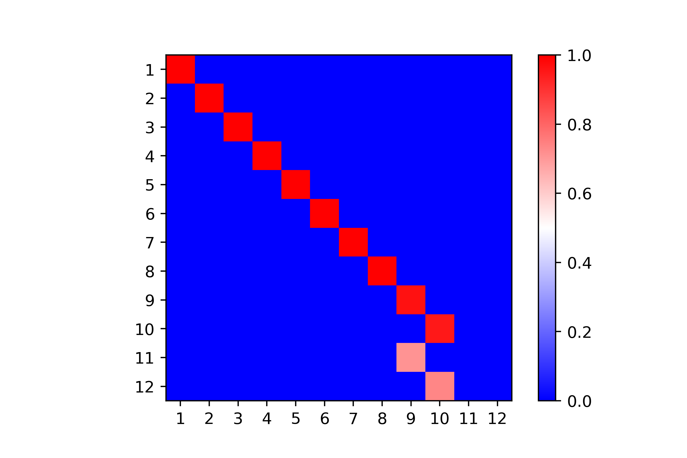
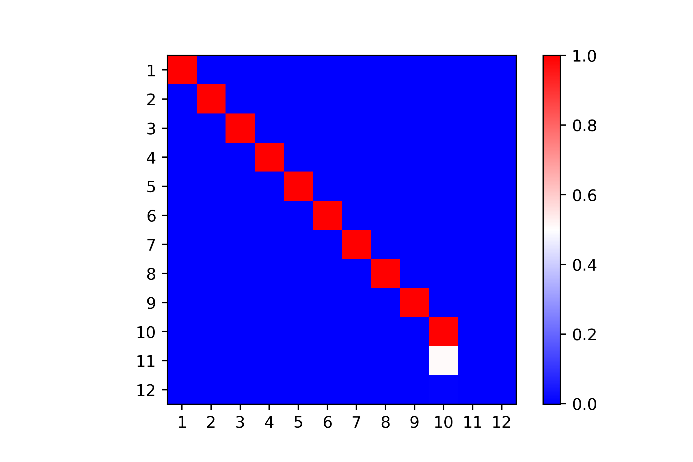
Figure 2. Spurious minima of optimization problem (1) under the Frobenius norm and with problem parameters $d=k=12,~{}n=5$ and $T=\sum_{i=1}^{k}\mathbf{e}_{i}^{\otimes{}5}$. (Left) a spurious minimum of isotropy $\Delta(S_{8}\times\langle(9~{}10)(11~{}12)\rangle)$. (Right) a spurious minimum of isotropy $\Delta(S_{9}\times S_{1}^{3})$.

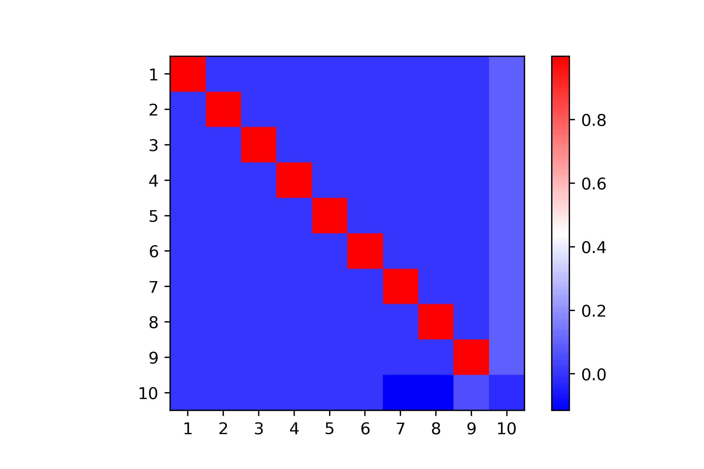
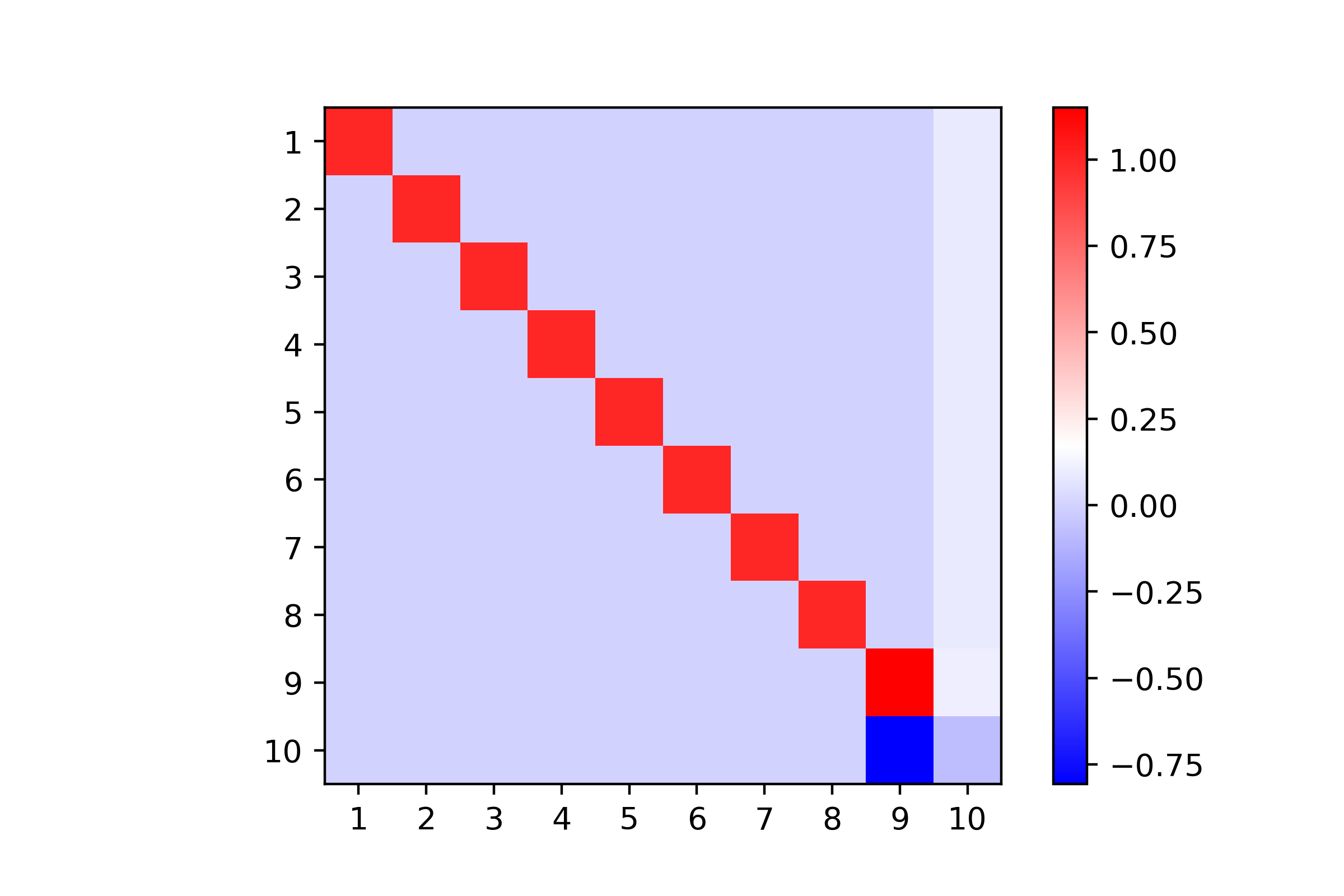
Figure 3. Spurious minima of optimization problem (1) under the cubic-Gaussian norm and problem parameters $d=k=10,~{}n=3$ and $T=\sum_{i=1}^{d}\mathbf{e}_{i}^{\otimes{}3}$. (Left) a spurious minimum of isotropy $\Delta(S_{6}\times S_{2}\times S_{1}^{2})$. (Right) a spurious minimum of isotropy $\Delta(S_{8}\times S_{1}^{2})$.

Convolutional target tensor

We now consider convolutional target tensors, demonstrating in particular symmetry breaking for non-identity target tensors. Specifically, we study problem (1) with target tensor $T_{\text{Lap}}:=\sum_{i=1}^{d}\mathbf{v}_{i}$, where $\mathbf{v}_{i}$ denote the rows of the circulant Laplacian-filter matrix

$$V_{\text{Lap}}:=\begin{pmatrix}-2&1&0&\cdots&0&1\\ \\ &\ddots&&\ddots&&\\ \\ 1&0&\cdots&0&1&-2\\ \end{pmatrix}.$$ (23)

The circulant structure of $V_{\text{Lap}}$ gives a $\Delta\mathbb{Z}_{d}$-isotropy, corresponding to convolutional filters used in contemporary artificial neural network architectures. Spurious minima obtained by repeating the training procedure described earlier exhibit, consistently over all runs, large isotropy subgroups of $S_{d}\times\mathbb{Z}_{d}$. An example of an approximated critical point is given in Figure 4.

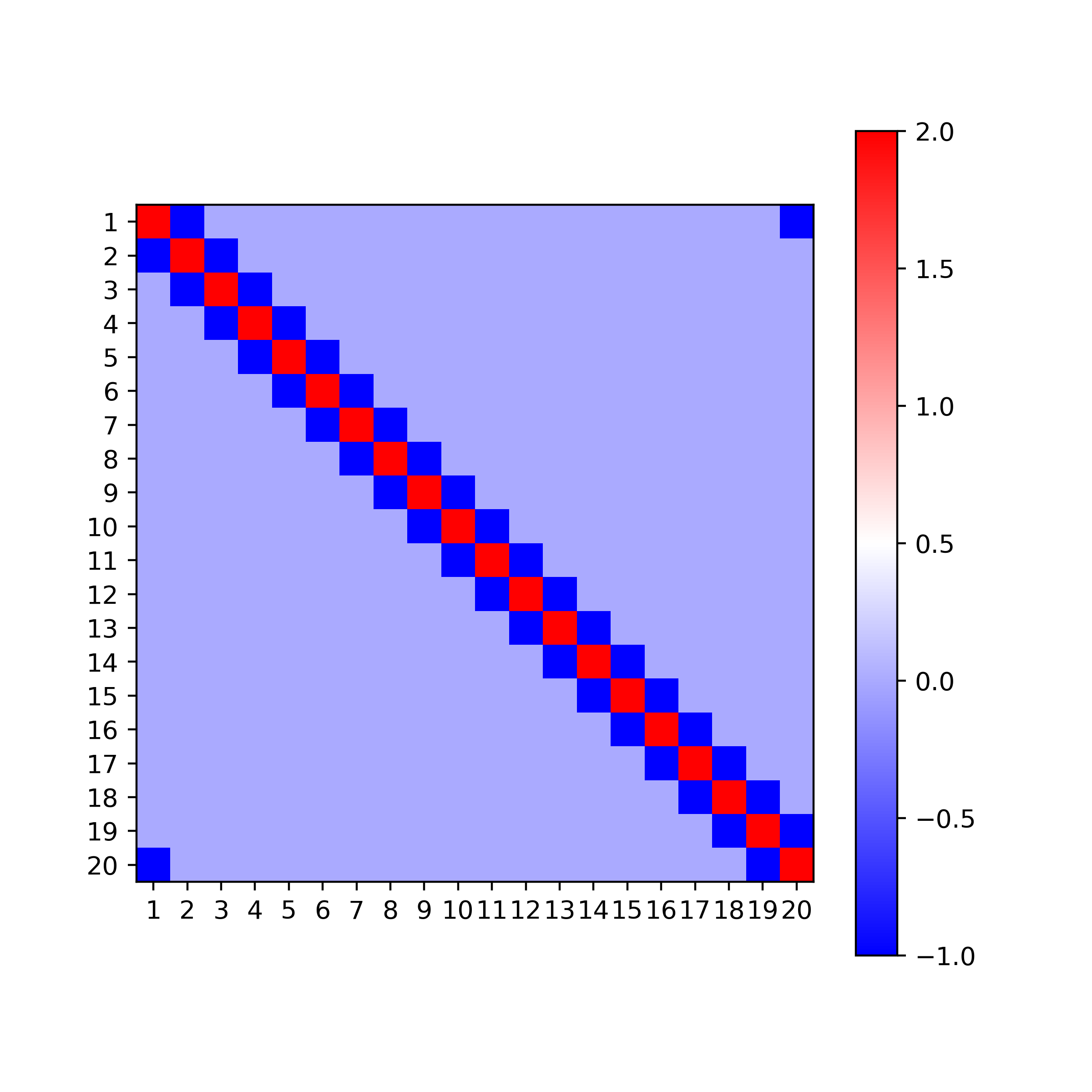
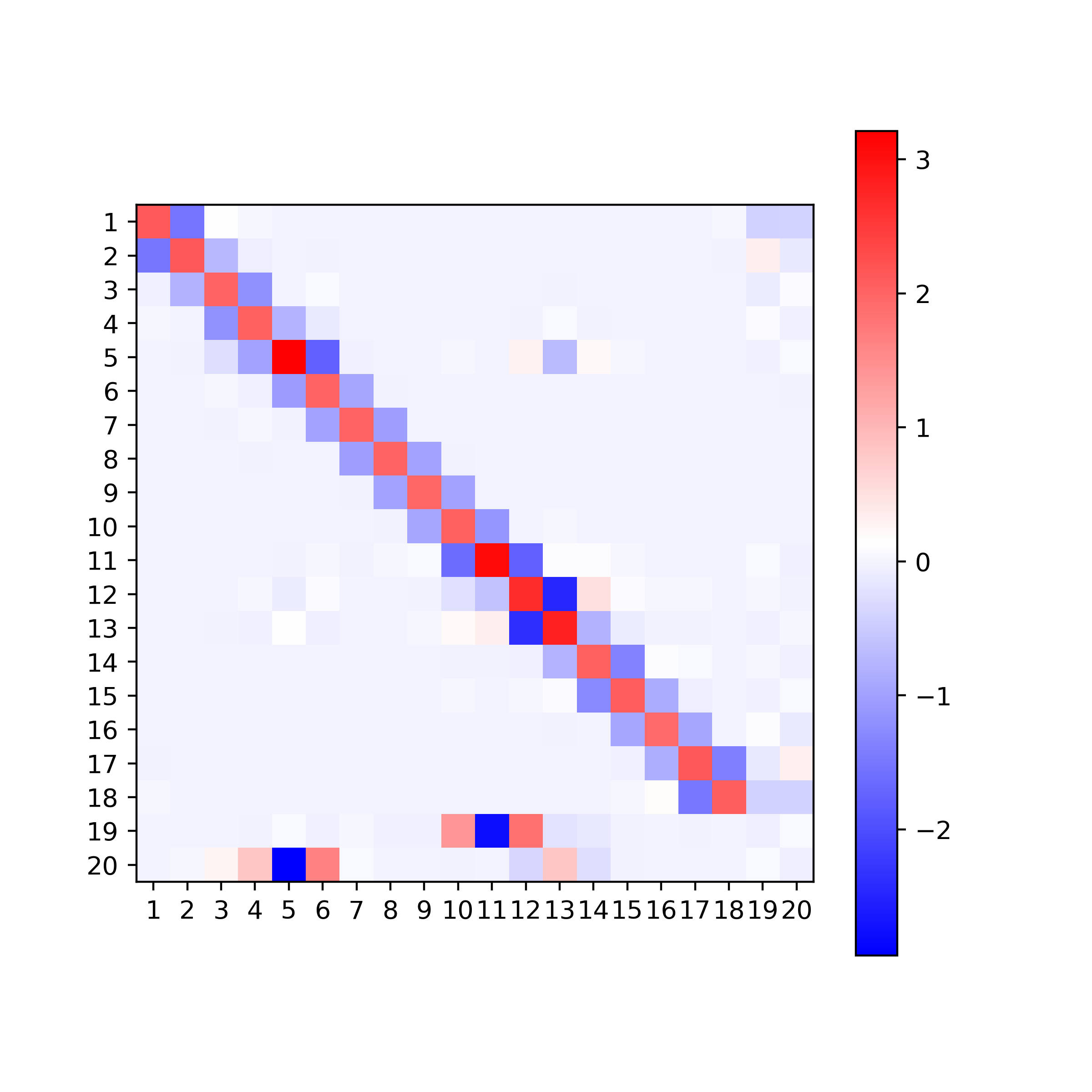
Figure 4. An approximated critical point of ${\mathcal{L}}_{\mathcal{N}}$ for $d=k=20$ and the Laplacian target tensor $T_{\text{Lap}}$. (Left) the target weight matrix $V_{\text{Lap}}$. (Right) a critical point computed numerically (with gradient norm $<1\mathrm{e-}2$)

5. Conclusion

In this note, we present a numerical study indicating that symmetry breaking phenomena occur for symmetric tensor decomposition problems. Our formulation of the invariance properties of the loss function (18) subsumes a wide class of nonconvex kernel-like nonconvex optimization problems. A particular implication is that symmetry breaking phenomena of the nature studied in this work applies more generally than for two layer ReLU networks, the setting in which the phenomenon was first observed. The numerical results provided were later used in [8] to study and characterize infinite families of critical points.

References

- [1] P. Comon, “Tensor decompositions,” Mathematics in Signal Processing V, pp. 1–24, 2002.
- [2] P. Comon and M. Rajih, “Blind identification of under-determined mixtures based on the characteristic function,” Signal Processing, vol. 86, no. 9, pp. 2271–2281, 2006.
- [3] L. De Lathauwer, B. De Moor, and J. Vandewalle, “A multilinear singular value decomposition,” SIAM Journal on Matrix Analysis and Applications, vol. 21, no. 4, pp. 1253–1278, 2000.
- [4] T. G. Kolda and B. W. Bader, “Tensor decompositions and applications,” SIAM Review, vol. 51, no. 3, pp. 455–500, 2009.
- [5] N. D. Sidiropoulos, R. Bro, and G. B. Giannakis, “Parallel factor analysis in sensor array processing,” IEEE Transactions on Signal Processing, vol. 48, no. 8, pp. 2377–2388, 2000.
- [6] A. Smilde, R. Bro, and P. Geladi, Multi-Way Analysis: Applications in the Chemical Sciences. John Wiley & Sons, 2005.
- [7] J. Landsberg, Tensors: Geometry and Applications: Geometry and Applications. Volume 128 of Graduate Studies in Mathematics, American Mathematical Society, 2011.
- [8] Y. Arjevani and G. Vinograd, “Symmetry & critical points for symmetric tensor decompositions problems,” arXiv preprint arXiv:2306.5319838, 2023.
- [9] T. G. Kolda, “Numerical optimization for symmetric tensor decomposition,” Mathematical Programming, vol. 151, no. 1, pp. 225–248, 2015.
- [10] N. Vervliet, O. Debals, L. Sorber, M. Van Barel, and L. De Lathauwer Tensorlab 3.0, Available online, Mar. 2016.
- [11] B. W. Bader, T. G. Kolda, et al. Tensor Toolbox for MATLAB, Version 3.2, www.tensortoolbox.org, February 10, 2021.
- [12] J. Nie, “Generating polynomials and symmetric tensor decompositions,” Foundations of Computational Mathematics, vol. 17, no. 2, pp. 423–465, 2017.
- [13] “Foundations of the PARAFAC procedure: models and conditions for an “explanatory” multimodal factor analysis,” UCLA Working Papers in Phonetics, vol. 16, pp. 1–84, 1970.
- [14] L. De Lathauwer, J. Castaing, and J.-F. Cardoso, “Fourth-order cumulant-based blind identification of underdetermined mixtures,” IEEE Transactions on Signal Processing, vol. 55, no. 6, pp. 2965–2973, 2007.
- [15] S. B. Hopkins, T. Schramm, and J. Shi, “A robust spectral algorithm for overcomplete tensor decomposition,” in Conference on Learning Theory, pp. 1683–1722, PMLR, 2019.
- [16] J. Kileel and J. M. Pereira, “Subspace power method for symmetric tensor decomposition and generalized PCA,” arXiv preprint arXiv:1912.04007, 2019.
- [17] S. Sherman and T. G. Kolda, “Estimating higher-order moments using symmetric tensor decomposition,” SIAM Journal on Matrix Analysis and Applications, vol. 41, no. 3, pp. 1369–1387, 2020.
- [18] Y. Arjevani and M. Field, “On the principle of least symmetry breaking in shallow ReLU models,” arXiv preprint arXiv:1912.11939, 2019.
- [19] Y. Arjevani and M. Field, “Symmetry & critical points for symmetric tensor decomposition problems,” 2022.
- [20] Y. Arjevani and M. Field, “Symmetry & critical points for a model shallow neural network,” Physica D: Nonlinear Phenomena, vol. 427, p. 133014, 2021.
- [21] Y. Arjevani and M. Field, “Analytic characterization of the hessian in shallow relu models: A tale of symmetry,” Advances in Neural Information Processing Systems, vol. 33, pp. 5441–5452, 2020.
- [22] Y. Arjevani and M. Field, “Analytic study of families of spurious minima in two-layer relu neural networks: a tale of symmetry ii,” Advances in Neural Information Processing Systems, vol. 34, pp. 15162–15174, 2021.
- [23] Y. Arjevani and M. Field, “Annihilation of spurious minima in two-layer relu networks,” Advances in Neural Information Processing Systems, vol. 35, pp. 37510–37523, 2022.
- [24] Y. Arjevani and M. Field, “Equivariant bifurcation, quadratic equivariants, and symmetry breaking for the standard representation of s k,” Nonlinearity, vol. 35, no. 6, p. 2809, 2022.
- [25] Y. Arjevani, “Hidden minima in two-layer relu networks,” arXiv preprint arXiv:2312.06234, 2023.
- [26] Y. Arjevani, J. Bruna, M. Field, J. Kileel, M. Trager, and F. Williams, “Symmetry breaking in symmetric tensor decomposition,” arXiv preprint arXiv:2103.06234, 2021.
- [27] L. Isserlis, “On a formula for the product-moment coefficient of any order of a normal frequency distribution in any number of variables,” Biometrika, vol. 12, no. 1/2, pp. 134–139, 1918.