HU-EP-21/05-RTG

Virtual corrections to $gg\to ZH$ via a transverse momentum expansion

Lina Alasfar^a, Giuseppe Degrassi^b, Pier Paolo Giardino^c, Ramona Gröber^d, Marco Vitti^b

(a) Humboldt-Universität zu Berlin, Institut für Physik, D-12489 Berlin, Germany
(b) Dipartimento di Matematica e Fisica, Università di Roma Tre and
INFN, sezione di Roma Tre, I-00146 Rome, Italy
(c) Instituto Galego de Física de Altas Enerxías, Universidade de Santiago de Compostela, 15782 Santiago de Compostela, Galicia-Spain
(d) Dipartimento di Fisica e Astronomia ’G. Galilei’, Università di Padova and INFN, sezione di Padova, I-35131 Padova, Italy

We compute the next-to-leading virtual QCD corrections to the partonic cross section of the production of a Higgs boson in association with a $Z$ boson in gluon fusion. The calculation is based on the recently introduced method of evaluating the amplitude via an expansion in terms of a small transverse momentum. We generalize the method to the case of different masses in the final state and of a process not symmetric in the forward-backward direction exchange. Our analytic approach gives a very good approximation (better than percent) of the partonic cross section in the center of mass energy region up to $\sim 750\,\textrm{GeV}$, where at the LHC $\sim 98\%$ of the total hadronic cross section is concentrated.

1 Introduction

The study of the characteristics of the Higgs boson is one of the primary tasks of the LHC program: the forthcoming Run3 and the High-Luminosity phase will increase the accuracy in the measurement of Higgs production cross sections and decay rates, allowing for a more stringent test of the Standard Model (SM) predictions. One of the main production processes being investigated is the so called Higgs-strahlung process $pp\to VH$, in which a single Higgs boson is emitted together with a weak vector boson ($V=Z,W$). The leptonic decays of the weak boson can be exploited as a trigger for measurements of elusive Higgs decays. In particular, the decay $H\rightarrow b\bar{b}$ has been observed for the first time by ATLAS and CMS, using an analysis focused precisely on the associated production category [1, 2].

In this paper, we are interested in the associated production of a Higgs and a $Z$ boson. The theoretical predictions for $pp\rightarrow ZH$ are accurate at next-to-next-to-leading-order (NNLO) in QCD, and at next-to-leading-order (NLO) in the EW interactions [3]. The leading and next-to-leading contributions are connected to the $q\bar{q}$-initiated channel, allowing to interpret $pp\rightarrow ZH$ mainly as a Drell-Yan process [4, 5].

The gluon-initiated channel $gg\rightarrow ZH$ arises for the first time at NNLO in QCD. It is an $\mathcal{O}(\alpha_{\scriptscriptstyle S}^{2})$ correction, but the contribution from this process to the hadronic cross section is non-negligible because of the large gluon luminosity at the LHC. It has been shown that the relevance of $gg\rightarrow ZH$ is even more enhanced in the boosted kinematic regime, to the point of being comparable to the quark-initiated contribution near the $t\bar{t}$ threshold [6]. The factorization- and renormalization-scale uncertainties related to the gluon-induced process also affect significantly the uncertainty on the total $pp\rightarrow ZH$ cross section. This issue is specific to the $ZH$ final state, since the gluon-induced channel is absent in $pp\rightarrow WH$. The knowledge of the NLO corrections to $gg\rightarrow ZH$ would reduce the scale uncertainties, facilitating precision studies in the next runs of the LHC. The $gg\rightarrow ZH$ contribution is relevant also for New Physics (NP) studies, since it is sensible to both sign and magnitude of the top Yukawa coupling, dipole operators [7] and can receive additional contributions from new particles [8].

An improved knowledge of the SM prediction for the gluon-induced contribution is therefore very important both for precision measurements of $ZH$ production within the SM and for testing NP in this channel. The leading order (LO) contribution to the $gg\rightarrow ZH$ amplitude, given by one-loop diagrams, was computed exactly in refs.[9, 10]. At the NLO the virtual correction part contains two-loop multi-scale integrals that constitute, at present, an obstacle to an exact evaluation of the NLO contribution. Specifically, the corrections due to the two-loop box diagrams are still not known analytically. A first computation of the NLO terms was obtained in ref.[11] using an asymptotic expansion in the limit $m_{t}\rightarrow\infty$ and $m_{b}=0$, and pointed to a $K$-factor of about 100% with respect to the LO contribution. Soft gluon resummation has been performed in ref.[12] including next-to-leading logarithmic terms, and the result has been matched to the fixed NLO computation of ref.[11]. Finite top-quark-mass effects to $gg\rightarrow ZH$ have been investigated in ref.[13] using a combination of large-$m_{t}$ expansion (LME) and Padé approximants. In addition, a data-driven method to extract the non-Drell-Yan part of $pp\rightarrow ZH$, which is dominated by the gluon-induced contribution, has been proposed in ref.[14], exploiting the known relation between $WH$ and $ZH$ associated production when only the Drell-Yan component of the two processes is considered. A qualitative study focusing on patterns in the differential distribution has been conducted in ref.[15], where $2\rightarrow 2$ and $2\rightarrow 3$ LO matrix elements were merged and matched to improve the description of the kinematics.

Very recently, a new analytic computation of the NLO virtual contribution based on a high-energy expansion of the amplitude, supported by Padé approximants, and on an improved LME, has been carried out [16]. The results are in agreement with a new exact numerical study [17], in the energy regions where the expansions are legitimate. Nonetheless, an improvement on the analytic calculation is still desirable, since the heavy-top and the high-energy expansions do not cover well the region $350\,{\rm GeV}\lesssim\sqrt{\hat{s}}\lesssim 750\,{\rm GeV}$, where $\sqrt{\hat{s}}$ is the partonic center of mass energy. It should be remarked that this region provides a significant part of the hadronic cross section at the LHC, about 68%.

In this paper, we present an analytic calculation of the virtual NLO QCD corrections to the $gg\to ZH$ process that covers the region $\sqrt{\hat{s}}\lesssim 750\,{\rm GeV}$, which contributes about 98% to the hadronic cross section. The most difficult parts, i.e. the two-loop box diagrams, are computed in terms of a forward kinematics [18] via an expansion in the $Z$ (or Higgs) transverse momentum, $p_{\scriptscriptstyle T}$, while the rest of the virtual corrections is computed exactly. We remark that our calculation is complementary to the results of ref.[16], which covers the region of large transverse momentum of the $Z$. Furthermore, the merging of the two analyses allows an analytic evaluation of the NLO virtual corrections in $gg\to ZH$ in the entire phase space.

The paper is structured as follows: in the next section we introduce our notation and the definitions of the form factors in terms of which we express the amplitude. In section 3, we present the expansion of the amplitude in terms of the $Z$ transverse momentum. Section 4 is devoted to a discussion of the expected range of validity of the evaluation of the amplitude via a $p_{\scriptscriptstyle T}$-expansion, by comparing the exact result for the LO cross section with the $p_{\scriptscriptstyle T}$-approximated one. In section 5 we present an outline of our NLO computation, while the next section contains our NLO results. Finally we present our conclusions. The paper is complemented by two appendices. In appendix A, we report the explicit expressions for the orthogonal projectors we employ in the calculation. We present also the relation between our form factors and the ones used in ref.[16]. In appendix B, we report the exact results for the triangle and the reducible double-triangle contributions.

2 Definitions

In this section we introduce our definitions for the calculation of the NLO QCD corrections to the associated production of a Higgs and a $Z$ boson from gluon fusion.

The amplitude $g^{\mu}_{a}(p_{1})g^{\nu}_{b}(p_{2})\to Z^{\rho}(p_{3})H(p_{4})$ can be written as

$${\cal A}=i\sqrt{2}\frac{m_{\scriptscriptstyle Z}G_{\scriptscriptstyle F}\alpha_{\scriptscriptstyle S}(\mu_{R})}{\pi}\delta_{ab}\epsilon^{a}_{\mu}(p_{1})\epsilon^{b}_{\nu}(p_{2})\epsilon_{\rho}(p_{3})\hat{{\cal A}}^{\mu\nu\rho}(p_{1},p_{2},p_{3}),$$ (1)

$$\hat{{\cal A}}^{\mu\nu\rho}(p_{1},p_{2},p_{3})=\sum_{i=1}^{6}\mathcal{P}_{i}^{\mu\nu\rho}(p_{1},p_{2},p_{3}){\cal A}_{i}(\hat{s},\hat{t},\hat{u},m_{t},m_{\scriptscriptstyle H},m_{\scriptscriptstyle Z}),$$ (2)

where $G_{\scriptscriptstyle F}$ is the Fermi constant, $\alpha_{\scriptscriptstyle S}(\mu_{R})$ is the strong coupling constant defined at a scale $\mu_{R}$ and $\epsilon^{a}_{\mu}(p_{1})\epsilon^{b}_{\nu}(p_{2})\epsilon_{\rho}(p_{3})$ are the polarization vectors of the gluons and the $Z$ boson, respectively. The tensors $\mathcal{P}_{i}^{\mu\nu\rho}$ are a set of orthogonal projectors, whose explicit expressions are presented in appendix A. The corresponding form factors ${\cal A}_{i}(\hat{s},\hat{t},\hat{u},m_{t},m_{\scriptscriptstyle H},m_{\scriptscriptstyle Z})$ are functions of the masses of the top quark ($m_{t}$), Higgs ($m_{\scriptscriptstyle H}$) and $Z$ ($m_{\scriptscriptstyle Z}$) bosons, and of the partonic Mandelstam variables

$$\hat{s}=(p_{1}+p_{2})^{2},~{}~{}\hat{t}=(p_{1}+p_{3})^{2},~{}~{}\hat{u}=(p_{2}+p_{3})^{2},$$ (3)

where $\hat{s}+\hat{t}+\hat{u}=m_{\scriptscriptstyle Z}^{2}+m_{\scriptscriptstyle H}^{2}$ and we took all the momenta to be incoming.

The ${\cal A}_{i}$ form factors can be expanded up to NLO terms as

$${\cal A}_{i}={\cal A}_{i}^{(0)}+\frac{\alpha_{\scriptscriptstyle S}}{\pi}{\cal A}_{i}^{(1)}$$ (4)

and the Born partonic cross section can be written as

$$\hat{\sigma}^{(0)}(\hat{s})=\frac{m_{\scriptscriptstyle Z}^{2}G_{\scriptscriptstyle F}^{2}\alpha_{\scriptscriptstyle S}(\mu_{R})^{2}}{64\hat{s}^{2}(2\pi)^{3}}\int^{\hat{t}^{+}}_{\hat{t}^{-}}d\hat{t}\sum_{i}\left|{\cal A}_{i}^{(0)}\right|^{2},$$ (5)

where $\hat{t}^{\pm}=[-\hat{s}+m_{\scriptscriptstyle H}^{2}+m_{\scriptscriptstyle Z}^{2}\pm\sqrt{(\hat{s}-m_{\scriptscriptstyle H}^{2}-m_{\scriptscriptstyle Z}^{2})^{2}-4m_{\scriptscriptstyle H}^{2}m_{\scriptscriptstyle Z}^{2}}\,]/2$.

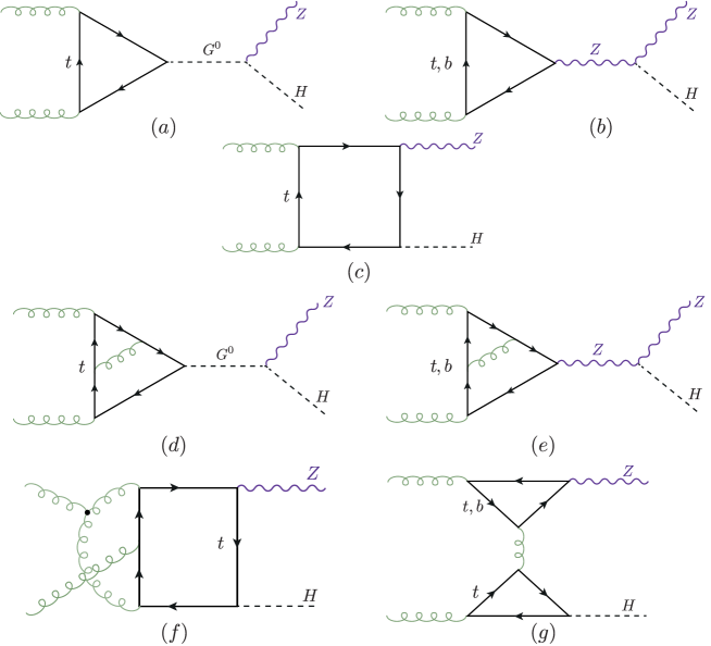
Figure 1: Examples of Feynman diagrams contributing to $gg\to ZH$ at LO and NLO.

The Feynman diagrams that contribute to the $gg\to ZH$ amplitude up to NLO can be separated into triangle, box and double-triangle contributions, the last type appearing for the first time at the NLO level. Examples of LO (NLO) triangle and box categories are shown in fig.1 $(a)$ - $(c)$ ($(d)$ - $(f)$). Due to the presence of a $\gamma_{5}$ in the axial coupling of the $Z$ boson to the fermions in the loop, the projectors $\mathcal{P}_{i}^{\mu\nu\rho}$ are proportional to the Levi-Civita total anti-symmetric tensor $\epsilon^{\alpha\beta\gamma\delta}$ (see appendix A), whose treatment in dimensional regularization is, as well known, delicate and will be discussed in section 5.

In our calculation we treat all the quarks but the top as massless. As a consequence, the contribution to the amplitude of the first two generations vanishes. Concerning the third generation, the contribution of the bottom is present in the triangle diagrams with the exchange of a $Z$ boson (fig.1$(b),(e)$) and in the double-triangle diagrams (fig.1$(g)$). A nice observation in ref.[11] allows to compute easily the full (top+bottom) triangle contribution. As noticed in that reference, the triangle contribution with a $Z$ exchange contains a $ggZ^{*}$ subamplitude which in the Landau gauge can be related to the decay of a massive vector boson with mass $\sqrt{\hat{s}}$ into two massless ones, a process that is forbidden by the Landau-Yang theorem [19, 20]. As a consequence, the full triangle contribution can be obtained from the top triangle diagrams with the exchange of the unphysical scalar $G^{0}$, with the propagator of the $G^{0}$ evaluated in the Landau gauge. This part of the top triangle diagrams can be obtained from the decay amplitude of a pseudoscalar boson into two gluons which is known in the literature in the full mass dependence up to NLO terms [21, 22].

Given the above observation, our calculation of the NLO corrections to the $gg\to ZH$ amplitude focuses on the analytic evaluation of the double-triangle (fig.1$(g)$) and two-loop box contributions (fig.1$(f)$). The former contribution is evaluated exactly. The latter is evaluated via two different expansions: i) via a LME, following ref.[23], up to and including ${\cal O}(1/m_{t}^{6})$ terms, which is expected to work below the $2\,m_{t}$ threshold; ii) via an expansion in terms of the $Z$ transverse momentum, following ref.[18], whose details are presented in the next section.

3 Expansion in the transverse momentum

The transverse momentum of the $Z$ boson can be written in terms of the Mandelstam variables as

$$p_{\scriptscriptstyle T}^{2}=\frac{\hat{t}\hat{u}-m_{\scriptscriptstyle Z}^{2}m_{\scriptscriptstyle H}^{2}}{\hat{s}}.$$ (6)

From eq.(6), together with the relation between the Mandelstam variables, one finds

$$p_{\scriptscriptstyle T}^{2}+\frac{m_{\scriptscriptstyle H}^{2}+m_{\scriptscriptstyle Z}^{2}}{2}\leq\frac{\hat{s}}{4}+\frac{\Delta_{m}^{2}}{\hat{s}},$$ (7)

where $\Delta_{m}=(m_{\scriptscriptstyle H}^{2}-m_{\scriptscriptstyle Z}^{2})/2$. Eq.(7) implies $p_{\scriptscriptstyle T}^{2}/\hat{s}<1$ that, together with the kinematical constraints $m_{\scriptscriptstyle H}^{2}/\hat{s}<1$ and $m_{\scriptscriptstyle Z}^{2}/\hat{s}<1$, allows the expansion of the amplitude in terms of these three ratios.

A direct expansion in $p_{\scriptscriptstyle T}$ is not possible at amplitude level, since $p_{\scriptscriptstyle T}$ itself does not appear in the amplitudes. However, as we argued in ref.[18], the expansion in $p_{\scriptscriptstyle T}^{2}/\hat{s}\ll 1$ is equivalent to an expansion in terms of the ratio of the reduced Mandelstam variables $t^{\prime}/s^{\prime}\ll 1$ or $u^{\prime}/s^{\prime}\ll 1$, depending whether we are considering the process to be in a forward or backward kinematics. The $s^{\prime},\,t^{\prime}$ and $u^{\prime}$ variables are defined as

$$s^{\prime}=p_{1}\cdot p_{2}=\frac{\hat{s}}{2},~{}~{}t^{\prime}=p_{1}\cdot p_{3}=\frac{\hat{t}-m_{\scriptscriptstyle Z}^{2}}{2},~{}~{}u^{\prime}=p_{2}\cdot p_{3}=\frac{\hat{u}-m_{\scriptscriptstyle Z}^{2}}{2}$$ (8)

and satisfy

$$s^{\prime}+t^{\prime}+u^{\prime}=\Delta_{m}.$$ (9)

The cross section of a $2\to 2$ process can always be expanded into a forward and backward contribution. Looking at the dependence of $\sigma$ upon $t^{\prime},\,u^{\prime}$ we can write

$$\sigma \propto \int^{t_{f}}_{t_{i}}dt^{\prime}\mathcal{F}(t^{\prime},u^{\prime})=\int^{t_{m}}_{t_{i}}dt^{\prime}\mathcal{F}(t^{\prime},u^{\prime})+\int^{t_{f}}_{t_{m}}dt^{\prime}\mathcal{F}(t^{\prime},u^{\prime})$$ (10)

$$\sim \int^{t_{m}}_{t_{i}}dt^{\prime}\mathcal{F}(t^{\prime}\sim 0,u^{\prime}\sim-s^{\prime})+\int^{t_{f}}_{t_{m}}dt^{\prime}\mathcal{F}(t^{\prime}\sim-s^{\prime},u^{\prime}\sim 0)$$

where $t_{i}=(\hat{t}^{-}-m_{\scriptscriptstyle Z}^{2})/2$, $t_{f}=(\hat{t}^{+}-m_{\scriptscriptstyle Z}^{2})/2$ and $t_{m}$ is the value of $t^{\prime}$ at which $t^{\prime}=u^{\prime}=(-s^{\prime}+\Delta_{m})/2$. The two terms in the second line of eq.(10) represent the expansion in the forward and backward kinematics, respectively.
If the amplitude is symmetric under $t^{\prime}\leftrightarrow u^{\prime}$ exchange then

$$\sigma \propto \int^{t_{m}}_{t_{i}}dt^{\prime}\mathcal{F}(0,-s^{\prime})+\int^{t_{f}}_{t_{m}}dt^{\prime}\mathcal{F}(-s^{\prime},0)=$$ (11)

$$\int^{t_{m}}_{t_{i}}dt^{\prime}\mathcal{F}(0,-s^{\prime})+\int^{t_{f}}_{t_{m}}dt^{\prime}\mathcal{F}(0,-s^{\prime})=\int^{t_{f}}_{t_{i}}dt^{\prime}\mathcal{F}(0,-s^{\prime})$$

so that the expansion in the forward kinematics actually covers the entire phase space.

In the case of $gg\to ZH$ the process itself is not symmetric under the $t^{\prime}\leftrightarrow u^{\prime}$ exchange. However, as can be seen from the explicit expressions of the projectors in appendix A, it can be written as a sum of symmetric and antisymmetric form factors. To perform only the expansion in the forward kinematics one can proceed in the following way. On the symmetric form factors the expansion can be directly performed. For the antisymmetric ones, it is sufficient first to extract the overall antisymmetric factor $(\hat{t}-\hat{u})$ just by multiplying the form factor by $1/(\hat{t}-\hat{u})$, written as $1/(2s^{\prime}-4t^{\prime}-2\Delta_{m})$, then perform the expansion in the forward kinematics and finally multiply back by $(\hat{t}-\hat{u})$.

As discussed in ref.[18], to implement the $p_{\scriptscriptstyle T}$-expansion at the level of Feynman diagrams it is convenient to introduce the vector $r^{\mu}=p_{1}^{\mu}+p_{3}^{\mu}$, which satisfies

$$r^{2}=\hat{t},~{}~{}r\cdot p_{1}=\frac{\hat{t}-m_{\scriptscriptstyle Z}^{2}}{2},~{}~{}r\cdot p_{2}=-\frac{\hat{t}-m_{\scriptscriptstyle H}^{2}}{2},$$ (12)

and therefore can be also written as

$$r^{\mu}=-\frac{\hat{t}-m_{\scriptscriptstyle H}^{2}}{\hat{s}}p_{1}^{\mu}+\frac{\hat{t}-m_{\scriptscriptstyle Z}^{2}}{\hat{s}}p_{2}^{\mu}+r_{\perp}^{\mu}=\frac{t^{\prime}}{s^{\prime}}\,(p_{2}^{\mu}-p_{1}^{\mu})-\frac{\Delta_{m}}{s^{\prime}}\,p_{1}^{\mu}+r_{\perp}^{\mu},$$ (13)

where

$$r_{\perp}^{2}=-p_{\scriptscriptstyle T}^{2}.$$ (14)

From eq.(6) one obtains

$$t^{\prime}=-\frac{s^{\prime}}{2}\left\{1-\frac{\Delta_{m}}{s^{\prime}}\pm\sqrt{\left(1-\frac{\Delta_{m}}{s^{\prime}}\right)^{2}-2\frac{p_{\scriptscriptstyle T}^{2}+m_{\scriptscriptstyle Z}^{2}}{s^{\prime}}}\right\}$$ (15)

that implies that the expansion in small $p_{\scriptscriptstyle T}$ (the minus sign case in eq.(15)) can be realized at the level of Feynman diagrams, by expanding the propagators in terms of the vector $r^{\mu}$ around $r^{\mu}\sim 0$ or, equivalently, $p_{3}^{\mu}\sim-p_{1}^{\mu}$, see eq.(13).

The outcome of the evaluation of the $gg\to ZH$ amplitude via a $p_{\scriptscriptstyle T}$-expansion is expressed in terms of a series of Master Integrals (MIs) that are functions of $\hat{s}$ and $m_{t}^{2}$ only, and whose coefficients can be organized in terms of powers of ratios of small over large parameters where $p_{\scriptscriptstyle T}^{2},\,m_{\scriptscriptstyle H}^{2}$ and $m_{\scriptscriptstyle Z}^{2}$ are identified as the small parameters while $m_{t}^{2}$ and $\hat{s}$ as the large ones. Thus, the range of validity of the expansion depends on the condition that $p_{\scriptscriptstyle T}^{2}$ can be treated as a “small parameter” with respect to $m_{t}^{2}$ because all the other ratios, small over large, are always smaller than 1.

4 LO Comparison

In order to investigate the range of validity of the evaluation of the $gg\to ZH$ amplitude via a $p_{\scriptscriptstyle T}$-expansion, we compare the exact result for the LO partonic cross section [9, 10] with the result obtained via our $p_{\scriptscriptstyle T}$-expansion. The latter is expressed in terms of the same four MIs that enter into the analogous calculation of the $gg\to HH$ LO amplitude [18], or

$$B_{0}[\hat{s},m_{t}^{2},m_{t}^{2}]\equiv B_{0}^{+}, B_{0}[-\hat{s},m_{t}^{2},m_{t}^{2}]\equiv B_{0}^{-},$$ (16)

$$C_{0}[0,0,\hat{s},m_{t}^{2},m_{t}^{2},m_{t}^{2}]\equiv C_{0}^{+}, ~{}~{}~{}C_{0}[0,0,-\hat{s},m_{t}^{2},m_{t}^{2},m_{t}^{2}]\equiv C_{0}^{-}$$ (17)

where

$$B_{0}[q^{2},m_{1}^{2},m_{2}^{2}]=\frac{1}{i\pi^{2}}\int\frac{d^{n}k}{\mu^{n-4}}\frac{1}{(k^{2}-m_{1}^{2})((k+q)^{2}-m_{2}^{2})}$$ (18)

$$C_{0}[q_{a}^{2},q_{b}^{2},(q_{a}+q_{b})^{2},m_{1}^{2},m_{2}^{2},m_{3}^{2}]=\hfill$$

$$\frac{1}{i\pi^{2}}\int\frac{d^{n}k}{\mu^{n-4}}\frac{1}{[k^{2}-m_{1}^{2}][(k+q_{a})^{2}-m_{2}^{2}][(k-q_{b})^{2}-m_{3}^{2}]}$$ (19)

are the Passarino-Veltman functions [24], with $n$ the dimension of spacetime and $\mu$ the ’t Hooft mass.

As an illustration of our LO result we present the explicit expressions for one symmetric, ${\cal A}_{2}$, and one antisymmetric, ${\cal A}_{6}$, form factor including the first correction in the ratio of small over large parameters which will be referred to as ${\mathcal{O}}(p_{\scriptscriptstyle T}^{2})$. We divide the result into triangle ($\triangle$) and box ($\square$) contribution or

$$\mathcal{A}_{2}^{(0,\triangle)} = -\frac{p_{\scriptscriptstyle T}}{\sqrt{2}\left(m_{\scriptscriptstyle Z}^{2}+p_{\scriptscriptstyle T}^{2}\right)}(\hat{s}-\Delta_{m})\,m_{t}^{2}C_{0}^{+},$$ (20)

$$\mathcal{A}_{2}^{(0,\square)} = \frac{p_{\scriptscriptstyle T}}{\sqrt{2}\left(m_{\scriptscriptstyle Z}^{2}+p_{\scriptscriptstyle T}^{2}\right)}\,\Biggl{\{}\Biggr{.}$$

$$\Biggl{(}m_{t}^{2}-m_{\scriptscriptstyle Z}^{2}\frac{\hat{s}-6m_{t}^{2}}{4\hat{s}}-p_{\scriptscriptstyle T}^{2}\frac{12m_{t}^{4}-16m_{t}^{2}\hat{s}+\hat{s}^{2}}{12\hat{s}^{2}}\Biggr{)}B_{0}^{+}$$

$$- \Biggl{(}m_{t}^{2}-\Delta_{m}\frac{m_{t}^{2}}{\left(4m_{t}^{2}+\hat{s}\right)}+m_{\scriptscriptstyle Z}^{2}\frac{24m_{t}^{4}-6m_{t}^{2}\hat{s}-\hat{s}^{2}}{4\hat{s}\left(4m_{t}^{2}+\hat{s}\right)}-$$

$$~{}~{}~{}~{}~{}~{}~{}p_{\scriptscriptstyle T}^{2}\frac{48m_{t}^{6}-68m_{t}^{4}\hat{s}-4m_{t}^{2}\hat{s}^{2}+\hat{s}^{3}}{12\hat{s}^{2}\left(4m_{t}^{2}+\hat{s}\right)}\Biggr{)}B_{0}^{-}$$

$$+ \Biggl{(}2m_{t}^{2}-\Delta_{m}+m_{\scriptscriptstyle Z}^{2}\frac{3m_{t}^{2}-\hat{s}}{\hat{s}}+p_{\scriptscriptstyle T}^{2}\frac{3m_{t}^{2}\hat{s}-2m_{t}^{4}}{\hat{s}^{2}}\Biggr{)}m_{t}^{2}\,C_{0}^{-}$$

$$+ \Biggl{(}\hat{s}-2m_{t}^{2}+m_{\scriptscriptstyle Z}^{2}\frac{\hat{s}-3m_{t}^{2}}{\hat{s}}+p_{\scriptscriptstyle T}^{2}\frac{2m_{t}^{4}-3m_{t}^{2}\hat{s}+\hat{s}^{2}}{\hat{s}^{2}}\Biggr{)}m_{t}^{2}\,C_{0}^{+}$$

$$+ \log\left(\frac{m_{t}^{2}}{\mu^{2}}\right)\frac{m_{t}^{2}}{\left(4m_{t}^{2}+\hat{s}\right)}\Biggl{(}\Delta_{m}+2m_{\scriptscriptstyle Z}^{2}+p_{\scriptscriptstyle T}^{2}\frac{2\hat{s}-2m_{t}^{2}}{3\hat{s}}\Biggr{)}$$

$$- \Delta_{m}\frac{2m_{t}^{2}}{\left(4m_{t}^{2}+\hat{s}\right)}+m_{\scriptscriptstyle Z}^{2}\frac{\hat{s}-12m_{t}^{2}}{4\left(4m_{t}^{2}+\hat{s}\right)}+p_{\scriptscriptstyle T}^{2}\frac{8m_{t}^{4}-2m_{t}^{2}\hat{s}+\hat{s}^{2}}{4\hat{s}(4m_{t}^{2}+\hat{s})}\Biggl{.}\Biggl{\}},$$

and

$$\mathcal{A}_{6}^{(0,\triangle)} = 0,$$ (22)

$$\mathcal{A}_{6}^{(0,\square)} = \frac{\hat{t}-\hat{u}}{\hat{s}^{2}}\,p_{\scriptscriptstyle T}\Biggl{[}\frac{m_{t}^{2}}{2}\Bigl{(}B_{0}^{-}-B_{0}^{+}\Bigr{)}-\frac{\hat{s}}{4}$$ (23)

$$- \frac{2m_{t}^{2}+\hat{s}}{2}m_{t}^{2}\,C_{0}^{-}+\frac{2m_{t}^{2}-\hat{s}}{2}m_{t}^{2}\,C_{0}^{+}\Biggr{]},$$

where in eqs.(LABEL:Adb,23) the $B_{0}$ functions are understood as the finite part of the integrals on the right hand side of eq.(18).

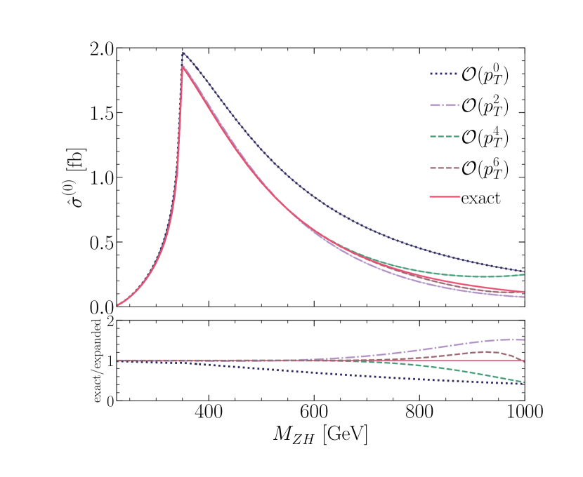
Figure 2: LO partonic cross section as a function of the invariant mass $M_{ZH}$. The full result (red line) is plotted together with results at different orders in the $p_{\scriptscriptstyle T}$-expansion (dashed lines). In the bottom part, the ratio of the full result over the $p_{\scriptscriptstyle T}$-expanded one at various orders is shown.

In fig.2 the exact partonic LO cross section (red line) is shown as a function of the invariant mass of the $ZH$ system, $M_{ZH}$, and compared to various $p_{\scriptscriptstyle T}$-expanded results. For the numerical evaluation of the cross section here and in the following, we used as SM input parameters

$$\begin{split}m_{\scriptscriptstyle Z}=91.1876\,\,\textrm{GeV},~{}~{}m_{\scriptscriptstyle H}=125.1\,\textrm{GeV},~{}~{}m_{t}=173.21\,\,\textrm{GeV},\\ m_{b}=0\,\,\textrm{GeV},~{}~{}G_{F}=1.16637\,\,\textrm{GeV}^{-2},~{}~{}\alpha_{s}(m_{\scriptscriptstyle Z})=0.118.\end{split}$$

In the lower part of fig.2 the ratio of the exact result over the $p_{\scriptscriptstyle T}$-expanded one is shown. From this ratio one can see that the $\mathcal{O}(p_{\scriptscriptstyle T}^{0})$ contribution covers well the $ZH$ invariant mass region $M_{ZH}\lesssim 2m_{t}$, corresponding to the range of validity of an expansion in the large top quark mass. Furthermore, when the contributions up to $\mathcal{O}(p_{\scriptscriptstyle T}^{4})$ are taken into account a remarkable agreement with the exact result is found up to $M_{ZH}\lesssim 750\,\textrm{GeV}$. This agreement is extended to sligthly higher values of $M_{ZH}$ when the $\mathcal{O}(p_{\scriptscriptstyle T}^{6})$ contribution is included, a finding in close analogy to the result for di-Higgs production [18]. Similar conclusions can be drawn from table 1, where it is shown that the partonic cross section at $\mathcal{O}(p_{\scriptscriptstyle T}^{4})$ agrees with the full result for $M_{ZH}\lesssim 600\,\textrm{GeV}$ on the permille level and the agreement further improves when $\mathcal{O}(p_{\scriptscriptstyle T}^{6})$ terms are included. As a final remark for this section, we notice that, from the comparison with the LO exact result, the $p_{\scriptscriptstyle T}$-expanded evaluation of the amplitude is expected to provide an accurate result up to $M_{ZH}\sim 700-750\,\textrm{GeV}$ that corresponds, from eq.(7), to $p_{\scriptscriptstyle T}\lesssim 300-350\,\,\textrm{GeV}\approx 2\,m_{t}$.

$M_{ZH}$ [GeV]	$\mathcal{O}(p_{\scriptscriptstyle T}^{0})$	$\mathcal{O}(p_{\scriptscriptstyle T}^{2})$	$\mathcal{O}(p_{\scriptscriptstyle T}^{4})$	$\mathcal{O}(p_{\scriptscriptstyle T}^{6})$	full
300	0.3547	0.3393	0.3373	0.3371	0.3371
350	1.9385	1.8413	1.8292	1.8279	1.8278
400	1.6990	1.5347	1.5161	1.5143	1.5142
600	0.8328	0.5653	0.5804	0.5792	0.5794
750	0.5129	0.2482	0.3129	0.2841	0.2919

Table 1: The partonic cross section $\hat{\sigma}^{(0)}$ at various orders in $p_{\scriptscriptstyle T}$ and the full computation for several values of $M_{ZH}$.

5 Outline of the NLO Computation

In this section we discuss our evaluation of the three different types of diagrams that appear in the virtual corrections to the $gg\to ZH$ amplitude at the NLO.

The triangle contribution (fig.1$(d),(e)$) was evaluated using the observation of ref.[11], i.e. we adapted the result of ref.[22] for the decay of a pseudoscalar boson into two gluons to our case. This contribution is evaluated exactly and explicit expressions for the form factors are presented in appendix B. We notice that if we interpret the exact result in terms of our counting of the expansion in $p_{\scriptscriptstyle T}$, the $p_{\scriptscriptstyle T}$-expansion of the triangle contribution stops at ${\cal O}(p_{\scriptscriptstyle T}^{2})$.

Given the reducible structure of the double-triangle diagrams (fig.1$(g)$), an exact result for the double-triangle contribution can be derived in terms of products of one-loop Passarino-Veltman functions [24]. Explicit expressions for this contribution are presented in appendix B. Although we write the amplitude using a different tensorial structure with respect to ref.[16] we checked, using the relations between the two tensorial structures reported in appendix A, that our result is in agreement with the one presented in ref.[13].

The box contribution (fig.1$(f)$) was computed evaluating the two-loop multi-scale Feynman integrals via two different expansions: a LME up to and including $\mathcal{O}(1/m_{t}^{6})$ terms, and an expansion in the transverse momentum up to and including ${\cal O}(p_{\scriptscriptstyle T}^{4})$ terms. The former expansion was used as “control” expansion of the latter. Indeed, the $p_{\scriptscriptstyle T}$-expanded result actually “contains” the LME one. The LME differs from the expansion in $p_{\scriptscriptstyle T}$ by the fact that $\hat{s}$ is treated as a small parameter with respect to $m_{t}^{2}$, and not on the same footing as in the latter case. This implies that if the $p_{\scriptscriptstyle T}$-expanded result is further expanded in terms of the $\hat{s}/m_{t}^{2}$ ratio the LME result has to be recovered. This way, we were able to reproduce, at the analytic level, our LME result.

We conclude this section outlining some technical details concerning our computation. We generated the amplitudes using FeynArts [25] and contracted them with the projectors as defined in appendix A using FeynCalc [26, 27] and in-house Mathematica routines. We used dimensional regularization and the rule for the contraction of two epsilon tensors written in terms of the determinant of $n$-dimensional metric tensors. This is not a consistent procedure and needs to be corrected. A correction term should be added [28] to the form factors computed as described above, ${\cal A}^{(1,ndr)}_{i}$, namely

$${\cal A}^{(1)}_{i}={\cal A}^{(1,ndr)}_{i}-\frac{\alpha_{\scriptscriptstyle S}}{\pi}C_{F}{\cal A}_{i}^{(0)}~{}.$$ (24)

In order to check eq.(24), following ref.[29] we bypassed the problem of the treatment of $\gamma_{5}$ in dimensional regularization computing the amplitude via a LME working in 4 dimension, employing the Background Field Method (BFM) [30] and using as regularization scheme the Pauli-Villars method. This result was compared with the LME evaluation of ${\cal A}^{(1,ndr)}_{i}$, finding that the difference between the two evaluations was indeed given by the second term on the right-hand-side of eq.(24).

After the contraction of the epsilon tensors the diagrams were expanded as described in section 3. They were reduced to MIs using FIRE [31] and LiteRed [32]. The resulting MIs were exactly the same as previously found for di-Higgs production [18]. Nearly all of them are expressed in terms of generalised harmonic polylogarithms with the exception of two elliptic integrals [33, 34]. The top quark mass was renormalized in the onshell scheme and the IR poles were subtracted as in ref.[35].

6 NLO results

We now present our numerical results for the virtual corrections. We have implemented our results into a FORTRAN programme. For the evaluation of the generalised harmonic polylogarithms we use the code handyG [36], while the elliptic integrals are evaluated using the routines of ref.[34]. In order to facilitate the comparison of our results with the ones presented in the literature, we define the finite part of the virtual corrections as in ref.[16]

$$\begin{split}\mathcal{V}_{fin}&=\frac{G_{F}^{2}m_{Z}^{2}}{16}\left(\frac{\alpha_{\scriptscriptstyle S}}{\pi}\right)^{2}\left[\sum_{i}\left|\mathcal{A}_{i}^{(0)}\right|^{2}\frac{C_{A}}{2}\left(\pi^{2}-\log^{2}\left(\frac{\mu_{R}^{2}}{\hat{s}}\right)\right)\right.\\ &\left.+2\sum_{i}\text{Re}\left[\mathcal{A}_{i}^{(0)}\left(\mathcal{A}_{i}^{(1)}\right)^{*}\right]\right]\,\end{split}$$ (25)

and in the numerical evaluation of eq.(25) we fixed $\mu_{R}=\sqrt{\hat{s}}$.

First, both the triangle and box LME contributions to $\mathcal{A}_{i}^{(1)}$ up to $\mathcal{O}(1/m_{t}^{6})$ terms were checked, at the analytic level, against the results of refs.[13, 16] finding perfect agreement. Then, the $p_{\scriptscriptstyle T}$-expanded results for low $M_{ZH}$ were confronted numerically with the LME ones, finding a good numerical agreement. We recall that, at the same order in the expansion, the $p_{\scriptscriptstyle T}$-expanded terms are more accurate than the LME ones, although computationally more demanding.

In ref.[17] a numerical evaluation of eq.(25) was presented. In that reference the exact NLO amplitude was reduced to a set of MIs that were evaluated numerically using the code pySecDec [37, 38]. Table 3 of that reference presents the numerical results for various points in the phase space. For the four points in that table lying within the range of validity of our expansion we find a difference with respect to our results of less than 1 permille in 3 cases and reaching the 1 permille level in one case, similarly to what we find at LO. It should be noticed that small differences on the permille level can be explained not only by the different approaches (exact vs. $p_{\scriptscriptstyle T}$-expanded) but also by the fact that in ref.[17] the $m_{\scriptscriptstyle Z}^{2}/m_{t}^{2}$ and $m_{\scriptscriptstyle H}^{2}/m_{t}^{2}$ ratios were approximated by a ratio of two integer numbers.

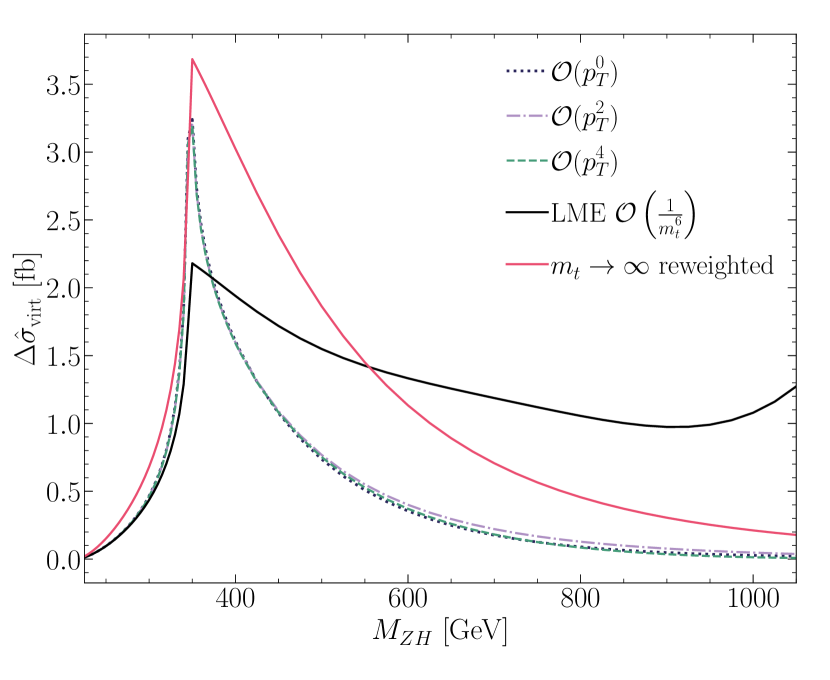
Figure 3: $\Delta\hat{\sigma}_{virt}$ defined by eq.(26), shown as a function of $M_{ZH}$. The various orders of the $p_{\scriptscriptstyle T}$-expansion are plotted as dashed lines, while the black and red continuous lines stand for the LME and reweighted $m_{t}\rightarrow\infty$ results, respectively.

In order to present our results we define a virtual part of the partonic cross section from the finite part of the virtual corrections in eq.(25) by

$$\Delta\hat{\sigma}_{virt}=\int_{\hat{t}^{-}}^{\hat{t}^{+}}d\hat{t}\frac{\alpha_{s}}{16\pi^{2}}\frac{1}{\hat{s}^{2}}\mathcal{V}_{fin}\,$$ (26)

and show it in fig.3. The dashed lines in the plot show the different orders in our expansion. For all parts of the matrix elements we use the best results available, i.e. both $\mathcal{A}^{(0)}$ and the double-triangle contribution are evaluated exactly, while for $\mathcal{A}^{(1)}$ we use the various orders in the $p_{\scriptscriptstyle T}$-expansion. For comparison, we show the results where $\mathcal{A}^{(1)}$ is replaced by the one computed in LME up to $\mathcal{O}(1/m_{t}^{6})$ (full black line), which as mentioned before is valid up to $M_{ZH}<2m_{t}$. We see that within the validity of the LME our results agree well with it. Furthermore, we show the results in the infinite top mass limit reweighted by the full amplitudes squared (full red line), corresponding to the approach of ref.[11], keeping though the double triangle contribution in full top mass dependence. Differently from the LME line, the $m_{t}\to\infty$ reweighted one shows a behaviour, for $M_{ZH}\gtrsim 400\,\textrm{GeV}$, similar to the behaviour of the $p_{\scriptscriptstyle T}$ lines. Still, the difference between the reweighted result and the $p_{\scriptscriptstyle T}$-expanded ones is significant. The $p_{\scriptscriptstyle T}$-expanded results show very good convergence. The zero order in our expansion agrees extremely well with the higher orders in the expansion, and all the three results are very close up to $M_{ZH}\sim 500\,\textrm{GeV}$.

Finally, we note that the evaluation of $\mathcal{V}_{fin}$ requires a running time per phase space point less than one second. In addition, the integration over the $\hat{t}$ variable in eq.(26) converges very well, such that fig.3 could be produced on a standard laptop in a few hours. Thus, our computation of the two-loop virtual corrections in $gg\to ZH$ is suitable to be used within a Monte Carlo code.

7 Conclusion

In this paper, we computed the two-loop NLO virtual corrections to the $gg\to ZH$ process. Among the two-loop Feynman diagrams contributing to the process, the ones belonging to the triangle and double-triangle topology were computed exactly. The ones belonging to the box topology, which contain multiscale integrals, were evaluated via an expansion in the $Z$ transverse momentum. This novel approach of computing a process in the forward kinematics was originally proposed in ref.[18] for double Higgs production where the particles in the final state have the same mass. In this paper, we extended the method to the more general case of two different masses in the final state and to a process whose amplitude is not symmetric under the $\hat{t}\leftrightarrow\hat{u}$ exchange.

The result of the evaluation of the box contribution is expressed, both at one- and two-loop level, in terms of the same set of MIs that was found in ref.[18] for double Higgs production. The two-loop MIs can be all expressed in terms of generalised harmonic polylogarithms with the exception of two elliptic integrals.

As we have shown explicitly at the LO, the range of validity of our computation covers values of the invariant mass $M_{ZH}\lesssim 750\text{ GeV}$ corresponding to 98.5% of the phase space at LHC energies. We showed that few terms in our expansion were sufficient to obtain an incredible good agreement with the numerical evalution of ${\mathcal{V}}_{fin}$ presented in ref.[17], at the level of a permille or less difference between our analytic result and the numerical one.

The advantage of our analytic approach compared to the numerical calculation is also in the computing time. With an average evaluation time of half a second per phase space point, an inclusion into a Monte Carlo programme is realistic. Due to the flexibility of our analytic results, an application to beyond-the-Standard Model is certainly possible.

Finally, we remark that our calculation complements nicely the results obtained in ref.[16] using a high-energy expansion, that according to the authors provides precise results for $p_{\scriptscriptstyle T}\gtrsim 200\,\textrm{GeV}$. The merging of the two analyses is going to provide a result that covers the whole phase space, can be easily implemented into a Monte Carlo code and presents the flexibility of an analytic calculation.

A Orthogonal Projectors in $gg\to ZH$

In this appendix we present the explicit expressions of the projectors $\mathcal{P}_{i}^{\mu\nu\rho}$ appearing in eq.(2). The projectors are all normalized to 1. They are:

$$\mathcal{P}_{1}^{\mu\nu\rho} = \frac{m_{\scriptscriptstyle Z}}{\sqrt{2}s^{\prime}p_{\scriptscriptstyle T}^{2}}\biggl{[}p_{1}^{\nu}\epsilon^{\mu\rho p_{1}p_{2}}-p_{2}^{\mu}\epsilon^{\nu\rho p_{1}p_{2}}+q_{t}^{\mu}\epsilon^{\nu\rho p_{2}p_{3}}$$ (A.1)

$$+ q_{u}^{\nu}\epsilon^{\mu\rho p_{1}p_{3}}+s^{\prime}\epsilon^{\mu\nu\rho p_{2}}-s^{\prime}\epsilon^{\mu\nu\rho p_{1}}\biggr{]},$$ (A.2)

$$\mathcal{P}_{2}^{\mu\nu\rho} = \frac{1}{\sqrt{2}s^{\prime}p_{\scriptscriptstyle T}}\biggl{[}q_{u}^{\nu}\epsilon^{\mu\rho p_{1}p_{3}}+q_{t}^{\mu}\epsilon^{\nu\rho p_{2}p_{3}}\biggr{]},$$ (A.3)

$$\mathcal{P}_{3}^{\mu\nu\rho} = \frac{\sqrt{3}}{2s^{\prime}p_{\scriptscriptstyle T}}\biggl{[}s^{\prime}\epsilon^{\mu\nu\rho p_{1}}+s^{\prime}\epsilon^{\mu\nu\rho p_{2}}-p_{1}^{\nu}\epsilon^{\mu\rho p_{1}p_{2}}-p_{2}^{\mu}\epsilon^{\nu\rho p_{1}p_{2}}$$ (A.4)

$$+ \left(q_{u}^{\nu}\epsilon^{\mu\rho p_{1}p_{3}}-q_{t}^{\mu}\epsilon^{\nu\rho p_{2}p_{3}}\right)\left(\frac{1}{3}+\frac{m_{\scriptscriptstyle Z}^{2}}{p_{\scriptscriptstyle T}^{2}}\right)$$

$$+ \frac{m_{\scriptscriptstyle Z}^{2}}{p_{\scriptscriptstyle T}^{2}}\left(q_{t}^{\mu}\epsilon^{\nu\rho p_{2}p_{1}}-q_{u}^{\nu}\epsilon^{\mu\rho p_{1}p_{2}}\right)\biggr{]},$$

$$\mathcal{P}_{4}^{\mu\nu\rho} = \frac{m_{\scriptscriptstyle Z}}{\sqrt{2}s^{\prime}p_{\scriptscriptstyle T}^{2}}\biggl{[}q_{t}^{\mu}(\epsilon^{\nu\rho p_{2}p_{1}}-\epsilon^{\nu\rho p_{2}p_{3}})-q_{u}^{\nu}(\epsilon^{\mu\rho p_{1}p_{2}}-\epsilon^{\mu\rho p_{1}p_{3}})\biggr{]},$$ (A.5)

$$\mathcal{P}_{5}^{\mu\nu\rho} = \frac{1}{\sqrt{6}s^{\prime}p_{\scriptscriptstyle T}}\biggl{[}q_{t}^{\mu}\epsilon^{\nu\rho p_{2}p_{3}}-q_{u}^{\nu}\epsilon^{\mu\rho p_{1}p_{3}}\biggr{]},$$ (A.6)

$$\mathcal{P}_{6}^{\mu\nu\rho} = \frac{1}{s^{\prime}p_{\scriptscriptstyle T}}\biggl{[}g^{\mu\nu}\epsilon^{\rho p_{1}p_{2}p_{3}}+s^{\prime}\epsilon^{\mu\nu\rho p_{3}}+p_{1}^{\nu}\epsilon^{\mu\rho p_{2}p_{3}}-p_{2}^{\mu}\epsilon^{\nu\rho p_{1}p_{3}}-\frac{s^{\prime}}{2}\epsilon^{\mu\nu\rho p_{2}}$$ (A.7)

$$+ \frac{1}{2}\left(p_{1}^{\nu}\epsilon^{\mu\rho p_{1}p_{2}}+p_{2}^{\mu}\epsilon^{\nu\rho p_{1}p_{2}}+q_{u}^{\nu}\epsilon^{\mu\rho p_{1}p_{3}}-q_{t}^{\mu}\epsilon^{\nu\rho p_{2}p_{3}}-s^{\prime}\epsilon^{\mu\nu\rho p_{1}}\right)$$

$$+ \frac{m_{\scriptscriptstyle Z}^{2}}{2p_{\scriptscriptstyle T}^{2}}(q_{t}^{\mu}\epsilon^{\nu\rho p_{2}p_{1}}-q_{u}^{\nu}\epsilon^{\mu\rho p_{1}p_{2}}+q_{u}^{\nu}\epsilon^{\mu\rho p_{1}p_{3}}-q_{t}^{\mu}\epsilon^{\nu\rho p_{2}p_{3}})\biggr{]}~{},$$

where we defined $q_{t}^{\mu}=(p_{3}^{\mu}-\frac{t^{\prime}}{s^{\prime}}p_{2}^{\mu})$ and $q_{u}^{\nu}=(p_{3}^{\nu}-\frac{u^{\prime}}{s^{\prime}}p_{1}^{\nu})$ and we used the shorthand notation $\epsilon^{\mu\nu\rho p_{2}}\equiv\epsilon^{\mu\nu\rho\sigma}p_{2}^{\sigma}$.

Using these projectors we obtained the relations between the form factors ${\cal A}_{i}$ defined in in eq.(2) and those defined in section 2 of ref.[16]:

$${\cal A}_{1} = \frac{p_{\scriptscriptstyle T}^{2}}{2\sqrt{2}m_{\scriptscriptstyle Z}(p_{\scriptscriptstyle T}^{2}+m_{\scriptscriptstyle Z}^{2})}\biggl{[}(t^{\prime}+u^{\prime})F_{12}^{+}-(t^{\prime}-u^{\prime})F_{12}^{-}\biggr{]},$$ (A.8)

$${\cal A}_{2} = -\frac{p_{\scriptscriptstyle T}}{2\sqrt{2}(p_{\scriptscriptstyle T}^{2}+m_{\scriptscriptstyle Z}^{2})}\biggl{[}(t^{\prime}+u^{\prime})F_{12}^{+}-(t^{\prime}-u^{\prime})F_{12}^{-}$$ (A.9)

$$- \frac{p_{\scriptscriptstyle T}^{2}+m_{\scriptscriptstyle Z}^{2}}{2s^{\prime}}((t^{\prime}+u^{\prime})F_{3}^{+}-(t^{\prime}-u^{\prime})F_{3}^{-})\biggr{]},$$

$${\cal A}_{3} = \frac{p_{\scriptscriptstyle T}}{2\sqrt{3}(p_{\scriptscriptstyle T}^{2}+m_{\scriptscriptstyle Z}^{2})}\biggl{[}(t^{\prime}+u^{\prime})F_{12}^{-}-(t^{\prime}-u^{\prime})F_{12}^{+}$$ (A.10)

$$+ (p_{\scriptscriptstyle T}^{2}+m_{\scriptscriptstyle Z}^{2})(F_{2}^{-}+F_{4})\biggr{]},$$

$${\cal A}_{4} = -\frac{m_{\scriptscriptstyle Z}}{2\sqrt{2}(p_{\scriptscriptstyle T}^{2}+m_{\scriptscriptstyle Z}^{2})}\biggr{[}(t^{\prime}+u^{\prime})F_{12}^{-}-(t^{\prime}-u^{\prime})F_{12}^{+}$$ (A.11)

$$+ (p_{\scriptscriptstyle T}^{2}+m_{\scriptscriptstyle Z}^{2})\left((1-\frac{p_{\scriptscriptstyle T}^{2}}{m_{\scriptscriptstyle Z}^{2}})F_{2}^{-}+2F_{4}\right)\biggl{]},$$

$${\cal A}_{5} = \frac{p_{\scriptscriptstyle T}}{2\sqrt{6}(p_{\scriptscriptstyle T}^{2}+m_{\scriptscriptstyle Z}^{2})}\biggr{[}(t^{\prime}+u^{\prime})F_{12}^{-}-(t^{\prime}-u^{\prime})F_{12}^{+}$$

$$+ (p_{\scriptscriptstyle T}^{2}+m_{\scriptscriptstyle Z}^{2})\left(4(F_{2}^{-}+F_{4})+\frac{3}{2s^{\prime}}\left((t^{\prime}+u^{\prime})F_{3}^{-}-(t^{\prime}-u^{\prime})F_{3}^{+}\right)\right)\biggr{]},$$

$${\cal A}_{6} = \frac{p_{\scriptscriptstyle T}}{2}F_{4}.$$ (A.13)

B Two-loop Results

The NLO amplitude can be written in terms of three contributions, namely the two-loop 1PI triangle, the two-loop 1PI box and the reducible double-triangle diagrams,

$$\mathcal{A}_{i}^{(1)}=\mathcal{A}_{i}^{(1,\triangle)}+\mathcal{A}_{i}^{(1,\square)}+\mathcal{A}_{i}^{(1,\bowtie)}~{}.$$ (B.1)

We present here the exact results for the double-triangle and triangle contributions to all the form factors. We find

$$\mathcal{A}_{1}^{(1,\bowtie)} = -\frac{m_{t}^{2}p_{\scriptscriptstyle T}^{2}}{4\sqrt{2}~{}m_{\scriptscriptstyle Z}\left(m_{\scriptscriptstyle Z}^{2}+p_{\scriptscriptstyle T}^{2}\right)^{2}}\Biggl{[}F_{t}(\hat{t})\left(G_{t}(\hat{t},\hat{u})-G_{b}(\hat{t},\hat{u})\right)+(\hat{t}\leftrightarrow\hat{u})\Biggr{]},$$ (B.2)

$$\mathcal{A}_{2}^{(1,\bowtie)} = \frac{m_{t}^{2}p_{\scriptscriptstyle T}}{4\sqrt{2}\left(m_{\scriptscriptstyle Z}^{2}+p_{\scriptscriptstyle T}^{2}\right)^{2}}\Biggl{[}F_{t}(\hat{t})\left(G_{t}(\hat{t},\hat{u})-G_{b}(\hat{t},\hat{u})\right)+(\hat{t}\leftrightarrow\hat{u})\Biggr{]},$$ (B.3)

$$\mathcal{A}_{3}^{(1,\bowtie)} = \frac{m_{t}^{2}p_{\scriptscriptstyle T}}{4\sqrt{3}~{}\hat{s}\left(m_{\scriptscriptstyle Z}^{2}+p_{\scriptscriptstyle T}^{2}\right)^{2}}\Biggl{[}\left(m_{\scriptscriptstyle H}^{2}-\hat{t}\right)F_{t}(\hat{t})\left(G_{t}(\hat{t},\hat{u})-G_{b}(\hat{t},\hat{u})\right)-(\hat{t}\leftrightarrow\hat{u})\Biggr{]},$$

$$\mathcal{A}_{4}^{(1,\bowtie)} = -\frac{m_{t}^{2}}{4\sqrt{2}~{}m_{\scriptscriptstyle Z}\hat{s}^{2}\left(m_{\scriptscriptstyle Z}^{2}+p_{\scriptscriptstyle T}^{2}\right)^{2}}\Biggl{[}\Bigl{(}m_{\scriptscriptstyle Z}^{2}\left(m_{\scriptscriptstyle H}^{2}-\hat{t}\right)^{2}$$ (B.5)

$$- \hat{t}\left(m_{\scriptscriptstyle Z}^{2}-\hat{u}\right)^{2}\Bigr{)}F_{t}(\hat{t})\left(G_{t}(\hat{t},\hat{u})-G_{b}(\hat{t},\hat{u})\right)-(\hat{t}\leftrightarrow\hat{u})\Biggr{]},$$

$$\mathcal{A}_{5}^{(1,\bowtie)} = -\frac{m_{t}^{2}p_{\scriptscriptstyle T}}{4\sqrt{6}~{}\hat{s}\left(m_{\scriptscriptstyle Z}^{2}+p_{\scriptscriptstyle T}^{2}\right)^{2}}\Biggl{[}\left(4m_{\scriptscriptstyle Z}^{2}-\hat{s}-4\hat{u}\right)F_{t}(\hat{t})\left(G_{t}(\hat{t},\hat{u})-G_{b}(\hat{t},\hat{u})\right)$$ (B.6)

$$- (\hat{t}\leftrightarrow\hat{u})\Biggr{]},$$

$$\mathcal{A}_{6}^{(1,\bowtie)} = 0,$$ (B.7)

where

$$F_{t}(\hat{t}) = \frac{1}{\left(m_{\scriptscriptstyle H}^{2}-\hat{t}\right)^{2}}\Biggl{[}2\hat{t}\Bigl{(}B_{0}\left(\hat{t},m_{t}^{2},m_{t}^{2}\right)-B_{0}\left(m_{\scriptscriptstyle H}^{2},m_{t}^{2},m_{t}^{2}\right)\Bigr{)}$$

$$+ \left(m_{\scriptscriptstyle H}^{2}-\hat{t}\right)\Bigl{(}\left(m_{\scriptscriptstyle H}^{2}-4m_{t}^{2}-\hat{t}\right)C_{0}\left(0,m_{\scriptscriptstyle H}^{2},\hat{t},m_{t}^{2},m_{t}^{2},m_{t}^{2}\right)-2\Bigr{)}\Biggr{]},$$

$$G_{x}(\hat{t},\hat{u}) = \left(m_{\scriptscriptstyle Z}^{2}-\hat{u}\right)\Biggl{[}m_{\scriptscriptstyle Z}^{2}\Bigl{(}B_{0}\left(\hat{t},m_{x}^{2},m_{x}^{2}\right)-B_{0}\left(m_{\scriptscriptstyle Z}^{2},m_{x}^{2},m_{x}^{2}\right)\Bigr{)}$$ (B.9)

$$+ \left(\hat{t}-m_{\scriptscriptstyle Z}^{2}\right)\Bigl{(}2m_{x}^{2}C_{0}\left(0,\hat{t},m_{\scriptscriptstyle Z}^{2},m_{x}^{2},m_{x}^{2},m_{x}^{2}\right)+1\Bigr{)}\Biggr{]}.$$

Instead, for the triangle diagrams, we obtain

$$\mathcal{A}_{1}^{(1,\triangle)} = \frac{p_{\scriptscriptstyle T}^{2}~{}(\hat{s}-\Delta_{m})}{4\sqrt{2}m_{\scriptscriptstyle Z}}\frac{\mathcal{K}_{t}^{(2l)}}{\left(p_{\scriptscriptstyle T}^{2}+m_{\scriptscriptstyle Z}^{2}\right)},$$ (B.10)

$$\mathcal{A}_{2}^{(1,\triangle)} = -\frac{p_{\scriptscriptstyle T}~{}(\hat{s}-\Delta_{m})}{4\sqrt{2}}\frac{\mathcal{K}_{t}^{(2l)}}{\left(p_{\scriptscriptstyle T}^{2}+m_{\scriptscriptstyle Z}^{2}\right)},$$ (B.11)

$$\mathcal{A}_{3}^{(1,\triangle)} = \frac{p_{\scriptscriptstyle T}~{}(\hat{t}-\hat{u})}{4\sqrt{3}}\frac{\mathcal{K}_{t}^{(2l)}}{\left(p_{\scriptscriptstyle T}^{2}+m_{\scriptscriptstyle Z}^{2}\right)},$$ (B.12)

$$\mathcal{A}_{4}^{(1,\triangle)} = -\frac{m_{\scriptscriptstyle Z}~{}(\hat{t}-\hat{u})}{4\sqrt{2}}\frac{\mathcal{K}_{t}^{(2l)}}{\left(p_{\scriptscriptstyle T}^{2}+m_{\scriptscriptstyle Z}^{2}\right)},$$ (B.13)

$$\mathcal{A}_{5}^{(1,\triangle)} = -\frac{p_{\scriptscriptstyle T}~{}(\hat{t}-\hat{u})}{4\sqrt{6}}\frac{\mathcal{K}_{t}^{(2l)}}{\left(p_{\scriptscriptstyle T}^{2}+m_{\scriptscriptstyle Z}^{2}\right)},$$ (B.14)

$$\mathcal{A}_{6}^{(1,\triangle)} = 0,$$ (B.15)

where the $\mathcal{K}_{t}^{(2l)}$ function is defined in eq.(4.11) of ref.[22].

We do not show the explicit results for the $p_{\scriptscriptstyle T}$-expansion of the two-loop box diagrams, since the analytic expressions are very lengthy, even for the lowest order term of the expansion.

References

- [1] ATLAS Collaboration, M. Aaboud et al., “Observation of decays and production with the ATLAS detector,” Phys. Lett. B 786 (2018) 59–86, arXiv:1808.08238 [hep-ex].
- [2] CMS Collaboration, A. M. Sirunyan et al., “Observation of Higgs boson decay to bottom quarks,” Phys. Rev. Lett. 121 no. 12, (2018) 121801, arXiv:1808.08242 [hep-ex].
- [3] S. Amoroso et al., “Les Houches 2019: Physics at TeV Colliders: Standard Model Working Group Report,” in 11th Les Houches Workshop on Physics at TeV Colliders: PhysTeV Les Houches. 3, 2020. arXiv:2003.01700 [hep-ph].
- [4] T. Han and S. Willenbrock, “QCD correction to the p p — W H and Z H total cross-sections,” Phys. Lett. B 273 (1991) 167–172.
- [5] O. Brein, A. Djouadi, and R. Harlander, “NNLO QCD corrections to the Higgs-strahlung processes at hadron colliders,” Phys. Lett. B 579 (2004) 149–156, arXiv:hep-ph/0307206.
- [6] C. Englert, M. McCullough, and M. Spannowsky, “Gluon-initiated associated production boosts Higgs physics,” Phys. Rev. D 89 no. 1, (2014) 013013, arXiv:1310.4828 [hep-ph].
- [7] C. Englert, R. Rosenfeld, M. Spannowsky, and A. Tonero, “New physics and signal-background interference in associated production,” EPL 114 no. 3, (2016) 31001, arXiv:1603.05304 [hep-ph].
- [8] R. V. Harlander, S. Liebler, and T. Zirke, “Higgs Strahlung at the Large Hadron Collider in the 2-Higgs-Doublet Model,” JHEP 02 (2014) 023, arXiv:1307.8122 [hep-ph].
- [9] B. A. Kniehl, “Associated Production of Higgs and Z Bosons From Gluon Fusion in Hadron Collisions,” Phys. Rev. D 42 (1990) 2253–2258.
- [10] D. A. Dicus and C. Kao, “Higgs Boson - Production From Gluon Fusion,” Phys. Rev. D 38 (1988) 1008. [Erratum: Phys.Rev.D 42, 2412 (1990)].
- [11] L. Altenkamp, S. Dittmaier, R. V. Harlander, H. Rzehak, and T. J. Zirke, “Gluon-induced Higgs-strahlung at next-to-leading order QCD,” JHEP 02 (2013) 078, arXiv:1211.5015 [hep-ph].
- [12] R. V. Harlander, A. Kulesza, V. Theeuwes, and T. Zirke, “Soft gluon resummation for gluon-induced Higgs Strahlung,” JHEP 11 (2014) 082, arXiv:1410.0217 [hep-ph].
- [13] A. Hasselhuhn, T. Luthe, and M. Steinhauser, “On top quark mass effects to at NLO,” JHEP 01 (2017) 073, arXiv:1611.05881 [hep-ph].
- [14] R. Harlander, J. Klappert, C. Pandini, and A. Papaefstathiou, “Exploiting the WH/ZH symmetry in the search for New Physics,” Eur. Phys. J. C 78 no. 9, (2018) 760, arXiv:1804.02299 [hep-ph].
- [15] B. Hespel, F. Maltoni, and E. Vryonidou, “Higgs and Z boson associated production via gluon fusion in the SM and the 2HDM,” JHEP 06 (2015) 065, arXiv:1503.01656 [hep-ph].
- [16] J. Davies, G. Mishima, and M. Steinhauser, “Virtual corrections to in the high-energy and large- limits,” arXiv:2011.12314 [hep-ph].
- [17] L. Chen, G. Heinrich, S. P. Jones, M. Kerner, J. Klappert, and J. Schlenk, “ production in gluon fusion: two-loop amplitudes with full top quark mass dependence,” arXiv:2011.12325 [hep-ph].
- [18] R. Bonciani, G. Degrassi, P. P. Giardino, and R. Gröber, “Analytical Method for Next-to-Leading-Order QCD Corrections to Double-Higgs Production,” Phys. Rev. Lett. 121 no. 16, (2018) 162003, arXiv:1806.11564 [hep-ph].
- [19] L. D. Landau, “On the angular momentum of a system of two photons,” Dokl. Akad. Nauk SSSR 60 no. 2, (1948) 207–209.
- [20] C.-N. Yang, “Selection Rules for the Dematerialization of a Particle Into Two Photons,” Phys. Rev. 77 (1950) 242–245.
- [21] M. Spira, A. Djouadi, D. Graudenz, and P. M. Zerwas, “Higgs boson production at the LHC,” Nucl. Phys. B 453 (1995) 17–82, arXiv:hep-ph/9504378.
- [22] U. Aglietti, R. Bonciani, G. Degrassi, and A. Vicini, “Analytic Results for Virtual QCD Corrections to Higgs Production and Decay,” JHEP 01 (2007) 021, arXiv:hep-ph/0611266.
- [23] G. Degrassi and P. Slavich, “NLO QCD bottom corrections to Higgs boson production in the MSSM,” JHEP 11 (2010) 044, arXiv:1007.3465 [hep-ph].
- [24] G. Passarino and M. J. G. Veltman, “One Loop corrections for annihilation into in the Weinberg Model,” Nucl. Phys. B160 (1979) 151.
- [25] T. Hahn, “Generating Feynman diagrams and amplitudes with FeynArts 3,” Comput. Phys. Commun. 140 (2001) 418–431, arXiv:hep-ph/0012260.
- [26] R. Mertig, M. Bohm, and A. Denner, “FEYN CALC: Computer algebraic calculation of Feynman amplitudes,” Comput. Phys. Commun. 64 (1991) 345–359.
- [27] V. Shtabovenko, R. Mertig, and F. Orellana, “New Developments in FeynCalc 9.0,” Comput. Phys. Commun. 207 (2016) 432–444, arXiv:1601.01167 [hep-ph].
- [28] S. Larin, “The Renormalization of the axial anomaly in dimensional regularization,” Phys. Lett. B 303 (1993) 113–118, arXiv:hep-ph/9302240.
- [29] G. Degrassi, S. Di Vita, and P. Slavich, “NLO QCD corrections to pseudoscalar Higgs production in the MSSM,” JHEP 08 (2011) 128, arXiv:1107.0914 [hep-ph].
- [30] L. F. Abbott, “The Background Field Method Beyond One Loop,” Nucl. Phys. B 185 (1981) 189–203.
- [31] A. V. Smirnov, “FIRE5: a C++ implementation of Feynman Integral REduction,” Comput. Phys. Commun. 189 (2015) 182–191, arXiv:1408.2372 [hep-ph].
- [32] R. N. Lee, “LiteRed 1.4: a powerful tool for reduction of multiloop integrals,” J. Phys. Conf. Ser. 523 (2014) 012059, arXiv:1310.1145 [hep-ph].
- [33] A. von Manteuffel and L. Tancredi, “A non-planar two-loop three-point function beyond multiple polylogarithms,” JHEP 06 (2017) 127, arXiv:1701.05905 [hep-ph].
- [34] R. Bonciani, G. Degrassi, P. P. Giardino, and R. Gröber, “A Numerical Routine for the Crossed Vertex Diagram with a Massive-Particle Loop,” Comput. Phys. Commun. 241 (2019) 122–131, arXiv:1812.02698 [hep-ph].
- [35] G. Degrassi, P. P. Giardino, and R. Gröber, “On the two-loop virtual QCD corrections to Higgs boson pair production in the Standard Model,” Eur. Phys. J. C 76 no. 7, (2016) 411, arXiv:1603.00385 [hep-ph].
- [36] L. Naterop, A. Signer, and Y. Ulrich, “handyG —Rapid numerical evaluation of generalised polylogarithms in Fortran,” Comput. Phys. Commun. 253 (2020) 107165, arXiv:1909.01656 [hep-ph].
- [37] S. Borowka, G. Heinrich, S. Jahn, S. P. Jones, M. Kerner, J. Schlenk, and T. Zirke, “pySecDec: a toolbox for the numerical evaluation of multi-scale integrals,” Comput. Phys. Commun. 222 (2018) 313–326, arXiv:1703.09692 [hep-ph].
- [38] S. Borowka, G. Heinrich, S. Jahn, S. P. Jones, M. Kerner, and J. Schlenk, “A GPU compatible quasi-Monte Carlo integrator interfaced to pySecDec,” Comput. Phys. Commun. 240 (2019) 120–137, arXiv:1811.11720 [physics.comp-ph].