Reservoir Computing as a Tool for Climate
Predictability Studies

Abstract

Reduced-order dynamical models play a central role in developing our understanding of predictability of climate irrespective of whether we are dealing with the actual climate system or surrogate climate-models. In this context, the Linear-Inverse-Modeling (LIM) approach, by capturing a few essential interactions between dynamical components of the full system, has proven valuable in providing insights into predictability of the full system.

We demonstrate that Reservoir Computing (RC), a form of learning suitable for systems with chaotic dynamics, provides an alternative nonlinear approach that improves on the predictive skill of the LIM approach. We do this in the example setting of predicting sea-surface-temperature in the North Atlantic in the pre-industrial control simulation of a popular earth system model, the Community-Earth-System-Model so that we can compare the performance of the new RC based approach with the traditional LIM approach both when learning data is plentiful and when such data is more limited. The improved predictive skill of the RC approach over a wide range of conditions—larger number of retained EOF coefficients, extending well into the limited data regime, etc.—suggests that this machine-learning technique may have a use in climate predictability studies. While the possibility of developing a climate emulator—the ability to continue the evolution of the system on the attractor long after failing to be able to track the reference trajectory—is demonstrated in the Lorenz-63 system, it is suggested that further development of the RC approach may permit such uses of the new approach in more realistic predictability studies.

Journal of Advances in Modeling Earth Systems (JAMES) Los Alamos National Lab, Los Alamos, NM 87544 B. T. Nadigabalu@lanl.gov

Plain Language Summary

Because of the chaotic nature of the dynamics underlying many complex systems such as weather and climate, evolution of ensembles of trajectories have to be considered in order to produce future predictions of such systems. An analysis of the dynamics of such ensembles provides insights into mechanisms that make the system predictable. Because comprehensive models of such complex systems are very costly to run, reduced order dynamical models of them are a useful tool in conducting such ensemble-based predictability studies. We develop such a computationally-inexpensive reduced order model using machine learning and show that it’s predictive skill is comparable to those of Linear Inverse Model (state of the art) when training data is plentiful, but much better when such data is more limited. Consequently we think that this new method has wide applicability. Furthermore, given the nonlinear nature of the new method, it has the potential to provide new insights into predictability of complex systems.

1 Introduction

Following the pioneering work of Lorenz (e.g., Lorenz, 1965, 1969, and others), understanding to what degree different aspects of the climate system are predictable has become a foundational aspect of climate science. Indeed, since predictability of climate can arise in two distinct ways, two kinds of predictability are identified and are of interest (Lorenz, 1975). In predictability of the first kind, predictability arises from variability internal to the climate system at various timescales when appropriately initialized and with error-growth/decorrelation from observations being controlled by the chaotic nature of the underlying dynamics. On the other hand, our ability to anticipate the response of the climate system to forcing external to the system, over a longer time scale gives rise to predictability of the second kind. However, since our ability to predict variations in climate as occurs due to internal/natural variability is much less developed than our ability to predict the response of the climate system to external forcing (e.g., see Stocker ., 2013, and references therein), we concern ourselves with tools to address issues related to predictability of the first kind in this article.

In the context of predictability of the first kind, because of the chaotic nature of climate dynamics, it is necessary to consider the evolution of an ensemble of trajectories be able to track the true trajectory of the climate system. However, since we are limited to observing the one climate system as it evolves, it is inevitable to have to use models to make progress on understanding predictability of the first kind. From the point of view of modeling, even if the probabilistic evolution of the climate system can be formulated correctly (e.g., as with the Liouville equation as in Ehrendorfer (1994)), the immense range of scales involved and the computational complexity of such a formulation renders it impractical and ensemble intergration of (severely) truncated models is the only feasible alternative. In any such model, while on the one hand, the difficulty of observationally estimating the state of the climate system inevitably leads to initial condition errors, the truncated representation of the climate system, on the other hand leads to model error. Here, by model error we refer to deficiencies in the model such as insufficient resolution and inaccurate parameterizations of unresolved processes which lead to the model’s inability to accurately simulate the delicate dynamical balance of processes that underlies both the mean state and the modes of variability of the climate system. Because of these errors—initial condition errors and model errors—model predictions invariably decorrelate rapidly from observations (e.g., see Nadiga, Verma ., 2019) and for this reason predictability studies have had to largely focus on so-called “perfect model” scenarios wherein a model trajectory is assumed to be the trajectory of interest (“true” trajectory) and the analysis of an ensemble of model integrations forms the basis for characterizing predictability.

Although imperfect, extensive investments in climate modeling over the past half a century have led to the development of a number of comprehensive climate models and Earth System Models (ESMs), and, they are proving invaluable in improving our understanding of various details of the climate system including its variability. The comprehensive nature of these models, however, renders them extremely resource-intensive, computationally and otherwise. Even as ensemble-based predictability studies with such models are beginning to be performed at great expense, the model-specific nature of such studies makes it difficult to relate the results of such studies to the actual climate system. To wit, while studies of the Atlantic Meridional Overturning Circulation (AMOC) in many models have found decadal to multidecadal predictability (e.g., see Griffies  Bryan, 1997; Pohlmann ., 2004; Collins ., 2006; Hawkins  Sutton, 2008; Sévellec ., 2008), these findings have tended to be disparate and model-specific, and establishing the relevance of such findings to the real system has been difficult.

A hierarchy of models, in terms of their complexity, has typically been important to advancing our understanding of various phenomena in climate science. For example, reduced-order dynamical models were central to Lorenz’s discovery of chaos and the ensuing body of work related to predictability Lorenz (e.g., Lorenz, 1965, 1969, and others). As such, it should not be surprising that reduced-order dynamical and empirical representations of comprehensive climate models and observations continue to serve as essential tools in our quest to further the understanding of predictability of climate today. One such reduced-order dynamical representation that has proved valuable is the Linear Inverse Model (LIM). While more fundamentally rooted in the fluctuation-dissipation theorem of equilibrium statistical mechanics, its typical usage in climate science follows the work of Hasselmann (Hasselmann, 1988) and Penland and co-workers (e.g., see Penland, 1989; Penland  Sardeshmukh, 1995; Farrell  Ioannou, 2001). The LIM approach consists of a linear dynamical system forced by white noise, where the linear dynamical operator and the covariance of the noise in a reduced dimensional space—typically Empirical Orthogonal Function (EOF) space are inferred from data. Indeed, predictions using the LIM approach have been shown to be skilful in a number of settings including the El Nino Southern Oscillation (ENSO) (e.g., see Penland  Magorian, 1993), the Pacific Decadal Oscillation (PDO) (e.g., see Newman, 2007; Alexander ., 2008), and the Atlantic Meridional Overturning Circulation (AMOC) (e.g., see Hawkins  Sutton, 2009).

Indeed, it is thought that the LIM approach is capable of capturing a large fraction of the predictable signal in a variety of settings. To wit, Newman  Sardeshmukh (2017), in analyzing the predictability of tropical sea surface temperature (SST) anomalies found that the forecast skill of a LIM derived from observed covariances of SST, sea surface height (SSH) and wind fields was close to that of the (fully nonlinear and first-principles based) operational North American Multi-Model Ensemble. The question then arises as to whether a linear approach, as with a LIM, captures the entirety of the predictable signal or as to whether there are predictable dynamics that are nonlinear and therefore not capturable in a linear framework. A first step towards exploring this issue consists of addressing the question of whether the predictive skill of the well established LIM methodology can be improved upon by further consideration of non-linearity. This will be the focus of the present article.

The issue of improving on the skill of the LIM approach by further consideration of nonlinearity itself has received substantial attention, although largely in the context of ENSO: Various authors ((e.g. Timmermann ., 2001; Kondrashov ., 2005, and others; also see Kondrashov . (2018))) have considered nonlinear extensions of LIMs, but the benefits of such extensions in terms of improved hindcast skill has been difficult to establish and generalize.

Given the successes of data-driven methods in fields such as computer vision, natural language processing, etc., over the past few decades, an alternative approach to considering, nonlinearity has been to adapt the artificial neural network (ANN) approach. While initial work in the area (e.g. Grieger  Latif, 1994; Hsieh  Tang, 1998, and others) was of an exploratory nature, later studies starting with (Tang ., 2000) show improved skill of the (nonlinear) ANN approach in comparison to linear methods (e.g., Ham ., 2019, and others).

In the context of methods relevant to predictability studies where we are interested in modeling temporal dynamics/processes, ANNs can be categorized as either feedforward neural networks (FNN) or recurrent neural networks (RNN). The use of feedforward networks in this setting leverages the capability of such networks to approximate a continuous function arbitrarily well (Cybenko, 1989) to learn the right hand side of an evolution operator. Here the evolution operator is typically related to an underlying (unknown) partial differential equation system if the system is considered in a physical domain or a set of ordinary differential equations if the system is considered in a modal domain and temporal evolution itself is achieved by the use of traditional time integration schemes (e.g., see Scher  Messori, 2019; Weyn ., 2019; DeGennaro ., 2019; Weyn ., 2020). Alternatively, an FNN can be used to directly learn the future state at a fixed time increment given its recent history. The latter RNN architecture, however, is distinguished by the presence of cyclical connections in how the neurons are connected (e.g., see Lukoševičius  Jaeger, 2009) and we concern ourselves with this architecture for the rest of this article. Such an RNN while featuring deterministic dynamics that transforms an input time series into an output time series through nonlinear filters, is capable of exhibiting self-sustained temporal dynamics.

In the context of RNNs, in response to various shortcomings of mainstream RNN architectures, an important one of which was the difficulty of training them, a new approach was proposed independently by Jaeger (2001) and Maass . (2002), and which has subsequently come to be known as Reservoir Computing (RC). In RC, an RNN that is randomly created and that remains unchanged during training—the reservoir—is passively excited by the input signal and maintains in the resevoir’s state a nonlinear transformation of the input history. Training then simply consists of using linear regression to obtain the weights that best give the desired output signal as a linear combination of the input and the resevoir state. In particular, since RC has outperformed other methods of nonlinear system identification, prediction, and classification in the context of chaotic dynamics (e.g., Jaeger  Haas, 2004; Pathak ., 2018, and others), we consider its use as a tool in climate predictability studies, while noting recent use of RC methods in the context of weather prediction (Arcomano ., 2020).

The rest of the article is structured as follows: In the next section we present the details of the problem we consider. Following that, in section 3, we present the Linear Inverse Model approach to the problem and discuss various details of the approach. After presenting details of the reservoir computing approach to the problem in section 4, we compare the results of this approach with the results of the LIM approach in section 5. A discussion of the results and some additional experiments using the Lorenz-63 system towards gaining some insight into the RC method and its performance in the climate setting are presented in section 6. A few implications of the study and a short discussion of the pros and cons of the new methodology then concludes the article.

2 Predictability of the North Atlantic Sea Surface Temperature

The utility of skilful near-term (subseasonal to decadal) predictions of regional climate is manifold and range from assessing societal and ecological impacts of a changing climate (e.g., see Council ., 2008; Adger, 2010) to planning and managing infrastructure (e.g., see Wilbanks  Fernandez, 2014) to insurance and risk management (e.g., see Mills, 2005) to adapt to such changes. In the framework of comprehensive climate and earth system models, a host of reasons, including the scientific challenges involved in being able to estimate the state of the climate system with sufficient accuracy and the complex, multiscale and chaotic dynamical nature of the climate system which complicates the process of accounting for uncertainty in the future evolution of errors in the initial state estimate, make predictions of the first kind more difficult than being able to model the response of the climate system to secular changes in external forcing such as due to greenhouse gases (e.g., see Meehl . (2009, 2014)). As such, our ability to produce longer term projections, projections that are contolled by external forcing related predictability, is better developed than our ability to produce near-term (subseasonal to decadal) predictions—predictions that are (increasingly) controlled by natural variability related predictability (as the prediction lead time decreases). It should, however, also be noted that the response of the climate system to external forcing can be/is modulated by natural variability, leading to the response to external forcing being amplified or mitigated on certain time scales of natural variability.

Remaining in the framework of comprehensive climate models, while initialized predictions of climate seek to augment the external forcing related predictability that is realized in uninitialized long term projections by predictability related to natural variability, there are a number of issues that remain to be resolved before such initialized predictions are skillful (e.g., see Kim ., 2012; Kharin ., 2012; Sanchez-Gomez ., 2016; Nadiga, Verma ., 2019). For example, in many such models observation based initialization in the presence of model bias leads to a rather rapid departure of the initialized prediction trajectory from observations necessitating post-processing of the predictions before they can show any skill at all. For these reasons, we concern ourselves with a statistical approach to the problem of near-term prediction of climate presently.

We consider the variability of SST in the North Atlantic over the last 800 years of the pre-industrial control (piControl; a simulation in which external forcing is held fixed) simulation of the Community Earth System Model (CESM2; Danabasoglu ., 2020) as part of the sixth phase of the Coupled Model Intercomparison Project (CMIP6). CESM2 is a global coupled ocean-atmosphere-land-land ice model and the piControl simulation we consider uses the Community Atmosphere Model (CAM6) and the Parallel Ocean Program (POP2), and at a nominal 1^o horizontal resolution in both the atmosphere and the ocean; the reader is referred to Danabasoglu . (2020) for details. This data is publicly available from the CMIP archive at https://esgf-node.llnl.gov/projects/cmip6 and its mirrors.

Two measures of predictability of SST in the North Atlantic are shown in Fig. 1. On the left is potential predictability and on the right is a decorrelation time. Potential predictability is defined as the ratio of the standard deviation of the N-year average of SST (in the current context) to the corresponding standard deviation of the 1-year average (Boer, 2004). As such, this measure assumes that variability on the longer (N$>$1) timescales is the signal related to potentially predictable processes (such as due to slow deterministic ocean dynamics) while that on the (faster) interannual scale is noise (attributable to processes such as chaotic internal variability). Potential predictability using a ten year average is shown in the left panel of Fig. 1.

Various definitions of decorrelation time ($\tau_{D}$) are possible (e.g., see Von Storch  Zwiers, 2001, and references therein) and three were considered:

$$\tau^{(1)}_{D}= 1+2\sum_{k=1}^{\infty}\rho(k),$$ (1)

$$\tau^{(2)}_{D}= 1+2\sum_{k=1}^{\infty}\rho^{2}(k),$$ (2)

and simply the e-folding time of the auto-correlation function $\rho(k)$ ($\tau^{(3)}_{D}=k$ at which $\rho(k)$ falls below $1/e$ for the first time). The computed values of $\tau^{(2)}_{D}$ and $\tau^{(3)}_{D}$ showed strong similarity with the former greater than the latter by about 20%, whereas $\tau^{(1)}_{D}$ showed a much larger range of values. For brevity and as a more conservative estimate of predictability, $\tau^{(3)}_{D}$ is shown in the right panel of Fig. 1. In this figure, the color bar for the decorrelation time is shown in months .

Both measures of predictability in Fig. 1 indicate that the more northern regions of the North Atlantic are more predictable, and that in these regions, predictability may extend to times as long as about eight years. We note that this finding is consistent with previous analysis of the variability of SST of the global ocean, both in observations and climate models that has identified the North Atlantic as a region that possesses significant predictability (Delworth  Mann, 2000; Boer, 2004; Hawkins ., 2011, and others). As such, we consider the spatio-temporal variability of SST in the North Atlantic for our example setting.

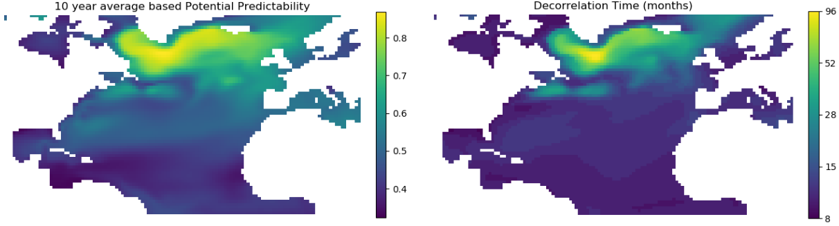
Figure 1: Two measures of predictability of SST in the North Atlantic. On the left is shown potential predictability computed as the pointwise ratio of the standard deviation of the ten year average to the standard deviation of the one year average. On the right is shown a measure of the decorrelation time computed as the pointwise e-folding time of the auto-correlation function. The time is shown in months on the colorbar.

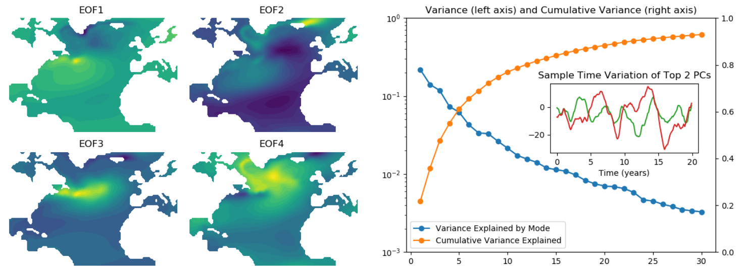
Figure 2: The leading EOFs of North Atlantic SST are shown on the left. Scale information is omitted since the EOFs are normalized. The main plot in the right panel shows the fraction of variance captured by individual modes (left axis) and the cumulative variance captured as a function of the mode number (right axis). The inset in the right panel shows time variations of the two leading principal components over a period of 20 years.

3 Linear Inverse Modeling

Since we are interested in predicting interannual variations of the SST based on data from the CESM2 simulation described above, we consider a twelve month moving-window average of the monthly SST field in what follows. The measures of predictability considered in the previous section were estimated in a spatially-local, pointwise fashion. A commonly used approach to further consider the effects of spatial covariance is that of empirial orthogonal function (EOF) analysis (equivalently principal component analysis PCA) (e.g., see Von Storch  Zwiers, 2001, and references therein). Furthermore, a truncated EOF basis also serves as an effective strategy to reduce the dimension of the system under consideration:

$$T({\mathbf{x}},t)=\sum_{k=1}^{N}e_{k}({\mathbf{x}})y_{k}(t),$$ (3)

where T is SST, $e_{k}({\mathbf{x}})$ is the $k-th$ EOF, $y_{k}(t)$ its corresponding time coefficient or principal component, and where $N$ the number of EOFs retained is much smaller than the number of spatial locations ${\mathbf{x}}$.

The spatial pattern of the first four EOFs on performing the analysis using the full record of 800 years is shown in the left panel of Fig. 2; scaling information/colorbars are omitted since the EOF patterns are normalized. The main plot in the right panel of Fig. 2 shows the fraction of variance captured by individual modes and the cumulative variance captured as a function of the mode number (using two separate vertical axes on the left and right respectively). While the first four modes capture about 50% of the variance, the first thirty modes capture about 95% of the variance. To give the reader a feel for the nature of temporal variability in the EOF basis, the inset in the right panel of Fig. 2 shows time variations of the two leading principal components (time coefficients) over a period of 20 years.

In its typical usage in climate science, the LIM approach consists of considering the evolution of the leading principal components as a linear dynamical system that is forced by white noise (e.g., see Hasselmann, 1988; Penland, 1989; Penland  Sardeshmukh, 1995; Farrell  Ioannou, 2001):

$$\frac{d{\mathbf{y}}}{dt}={\mathbf{B}}{\mathbf{y}}+\boldsymbol{\xi},$$ (4)

where ${\mathbf{y}}$ is the state vector, i.e., the truncated vector of principle components. In (4) ${\mathbf{B}}$ is a constant deterministic matrix determined as:

$${\mathbf{B}}=\frac{1}{\tau_{0}}\ln\left({\mathbf{C}}_{\tau_{0}}{\mathbf{C}}_{0}^{-1}\right),$$ (5)

where ${\mathbf{C}}_{\tau_{0}}=\left<{\mathbf{y}}(t+\tau_{0}){\mathbf{y}}^{T}(t)\right>$ is the lagged covariance at a chosen lag $\tau_{0}$, ${\mathbf{C}}_{0}=\left<{\mathbf{y}}(t){\mathbf{y}}^{T}(t)\right>$ is the (zero-lag) covariance, and $\boldsymbol{\xi}$ is a (vector) white noise process with a covariance matrix ${\mathbf{Q}}$ ($=\left<\boldsymbol{\xi}\boldsymbol{\xi}^{T}\right>$) that is determined from:

$${\mathbf{B}}{\mathbf{C}}_{0}+{\mathbf{C}}_{0}{\mathbf{B}}^{T}+{\mathbf{Q}}=0.$$ (6)

See Penland (1989) for details. The LIM (4), can then be used to predict ${\mathbf{y}}$ at lead time $\tau$ as

$${\mathbf{y}}_{L}(t+\tau)=\exp(\tau{\mathbf{B}}){\mathbf{y}}(t)+\exp(\tau{\mathbf{B}})\int_{t}^{t+\tau}\exp(-t^{\prime}{\mathbf{B}})\boldsymbol{\xi}(t^{\prime})dt^{\prime}.$$ (7)

However, if we are only interested in the ensemble average over realizations of the noise process, then

$$\bar{{\mathbf{y}}}_{L}(t+\tau)=\exp(\tau{\mathbf{B}}){\mathbf{y}}(t).$$ (8)

In the rest of the article, we’ll only consider the ensemble average prediction and drop the overbar for convenience:

$${\mathbf{y}}_{L}(t+\tau)=\exp(\tau{\mathbf{B}}){\mathbf{y}}(t)={\mathbf{P}}_{\tau}{\mathbf{y}}(t).$$ (9)

Here it is important to note that ${\mathbf{P}}_{\tau}$, the propagator of the state vector ${\mathbf{y}}$ over a period $\tau$ has to tend to zero at long lead times:

$$\lim\limits_{\tau\rightarrow\infty}\;{\mathbf{P}}_{\tau}=0$$ (10)

or equivalently that the real part of all of the eigenvalues of ${\mathbf{B}}$ have to be negative for the LIM to be useful.

Finally, if, the true dynamics of the system were indeed linear, the expected mean square error of the prediction ${\mathbf{y}}_{L}(t+\tau)$ at lead time $\tau$ is (related to the covariance of the (vector) noise process and) given by

$$\epsilon_{ifL}(\tau)=\frac{\hbox{tr}\left({\mathbf{C}}_{0}-{\mathbf{P}}_{\tau}{\mathbf{C}}_{0}{\mathbf{P}}^{T}_{\tau}\right)}{\hbox{tr}({\mathbf{C}}_{0})},$$ (11)

where tr($\cdot$) is the trace of the relevant matrix. However, since the actual evolution of the principal components of SST is likely nonlinear, a comparison of the actual error of the ensemble-averaged prediction ${\mathbf{y}}_{L}(t+\tau)$ in (9) to the theoretical estimate of the error if the actual evolution were to be linear in (11) can be used as a measure of nonlinearity in the actual evolution.

We end this section by noting a couple of alternative/complementary views of the LIM approach. While we presented the LIM approach here as a somewhat ad-hoc “reduced order modeling” approach, the methodology has deeper roots in statistical mechanics and dynamical systems theory. Indeed the SST prediction problem can be recast as one seeking, in effect, a global space-time response of a statistically steady surface ocean from a dynamical systems perspective. In this context, the Fluctuation Dissipation Theorem (FDT) of statistical mechanics relates the linear response of the system to certain space-time correlation functions of the undisturbed system (e.g., see Leith, 1975; Gritsun  Branstator, 2007; Abramov  Majda, 2007): The surface ocean is continuously experiencing small forcings of numerous different types, and these generate corresponding fluctuation responses. Therefore, given a sufficiently detailed space-time map of these correlations, the FDT allows the response to a given force to be extracted and resolved, leading exactly to the LIM formulation described above.

Alternatively, when used as a data-driven approach to approximate the evolution of an underlying nonlinear dynamical system, the LIM approach, in common with the Dynamical Mode Decomposition (DMD) approach (e.g., see Tu ., 2014), arises in the context of spectral analysis of the Koopman operator—a linear but infinite-dimensional operator whose modes and eigenvalues capture the evolution of observables describing any dynamical system, even nonlinear ones (e.g., see Tu ., 2014). In this context, (a) the propagator $P_{\tau}$ in (9) is the Koopman operator, on using the state vector itself as the observable. However, since the Koopman operator acts on functions rather than on the state itself, the Koopman operator steps the observation operator forward in time, and since the observation operator here is the identity operator, in effect the state is stepped forward in time, and (b) rather than thinking of $P_{\tau}$ as arising from a linearization of the underlying dynamics, it is better thought of as an average of the nonlinear dynamics evaluated over an ensemble of snapshots (e.g., see Blumenthal, 1991).

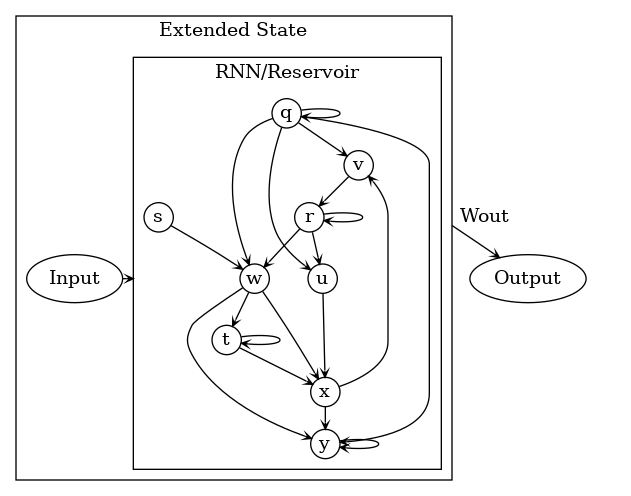
Figure 3: A schematic of the reservoir computing architecture. The connectivity between the neurons in the reservoir is random and training is limited to determining ${\mathbf{W}}_{out}$ using (a regularized form of) linear regression over the training data. In the prediction phase, the output becomes the input for the next time step.

4 Reservoir Computing

As mentioned in the introduction, Reservoir Computing is a form of Recurrent Neural Network (RNN) in which a randomly created reservoir stores a set of nonlinear transformations of the input signal and in which training consists of using linear regression to obtain the weights that best give the desired output signal as a linear combination of the input and the resevoir state (e.g., see Lukoševičius  Jaeger, 2009, and references therein).

Following the development in Lukoševičius  Jaeger (2009), in general, an RNN may be thought of as mapping a (vector) input time series ${\mathbf{u}}(n)$ to a (vector) output time series ${\mathbf{y}}(n)$ with $n=1,\ldots,T$, and e.g., as shown in schematic Fig. 3. We note here that when the dimensionality of the problem is reduced, as we do by using EOFs here, ${\mathbf{y}}(n)$ comprises of the time evolving coefficients of the retained modes. However, if such dimension reduction techniques were not employed, while ${\mathbf{y}}(n)$ would comprise of the temporally evolving values of relevant variables at different spatial locations, spatial-locality of the governing dynamics would lead us to consider separate reservoirs for each of the domain-decomposed neighborhoods with further exchange of (boundary or halo) information between adjoining reservoirs at regular time intervals. For the kinds of applications we consider in this article, it is natural to consider ${\mathbf{u}}(n)={\mathbf{y}}(n-1)$ (autonomous dynamics). (But for the difference that augmenting the input vector ${\mathbf{u}}(n)$ by a unit entry is a convenient way of including bias in both the reservoir update (see (14)) and in the readout (see (12)). As such, input and output in this article refer to the evolving state vector ${\mathbf{y}}$ at two subsequent time steps and where the time step is fixed at a month. Note that we refer to the vector ${\mathbf{y}}$ as the state vector, the vector ${\mathbf{r}}$ as the resevoir state (vector), and the combined vector {${\mathbf{r}},{\mathbf{y}}$} as the extended state (vector). Finally, when we mention input in the rest of the article, we refer to ${\mathbf{u}}(n)$ in the more general (non-autonomous) setting or to ${\mathbf{y}}(n)$ in the present (autonomous) setting.

4.1 Nonlinear Kernels and Linear Readout

Indeed, to investigate the possibility of improving on the Linear inverse modeling approach of the previous section, we are interested in going beyond ${\mathbf{y}}(n+1)={\mathbf{W}}{\mathbf{y}}(n)$ where (and in the rest of the article) ${\mathbf{W}}$ is a constant weight matrix. A generic approach to nonlinear modeling is to first consider transformation of the input ${\mathbf{y}}(n)$ into a high-dimensional set of nonlinear features ${\mathbf{r}}(n)$ and then apply linear techniques such as linear regression to obtain a nonlinear model. Following this approach in the present context leads to the nonlinear model

$${\mathbf{y}}(n+1)={\mathbf{W}}_{out}\tilde{{\mathbf{r}}}(n).$$ (12)

Here, again, ${\mathbf{W}}_{out}$ is a constant weight matrix of dimension $N_{y}\times N_{\tilde{r}}$, but with $N_{\tilde{r}}\gg N_{y}$ typically, and where $\tilde{{\mathbf{r}}}$ is the combined vector of ${\mathbf{r}}(n)$, the set of nonlinear features and ${\mathbf{y}}(n)$, the input: $\tilde{{\mathbf{r}}}=\left\{{\mathbf{r}}(n),{\mathbf{y}}(n)\right\}$, with $N_{\tilde{r}}=N_{r}+N_{u}$.

4.2 Recurrent Neural Networks

The storage of the nonlinear expansion/transformations of the input with memory in an RNN is given by the evolution of the RNN state as

$${\mathbf{r}}(n)=f\left({\mathbf{W}}{\mathbf{r}}(n-1)+{\mathbf{W}}_{in}{\mathbf{u}}(n)\right),n=1,\ldots,T,$$ (13)

where ${\mathbf{r}}(n)$ and ${\mathbf{u}}(n)$ are respectively the vector of RNN states and the vector of inputs at time step $n$, and $f(\cdot)$ is the activation function applied element-wise. In (13), ${\mathbf{W}}_{in}$ and ${\mathbf{W}}$ are both weight matrices with dimensions $N_{r}\times N_{u}$ and $N_{r}\times N_{r}$ respectively. We note here that the bias term in (13) is included by adding a unit entry to the input vector.

Indeed, a yet-simpler approximation that foregoes the connectivity between the neurons in the reservoir in (13) and relies entirely on random features to construct kernel machines has been considered by various authors (e.g., see Rahimi  Recht, 2008; Gottwald  Reich, 2020).

Finally, we note that, to account for certain details of the system such as the data frequency, (e.g., on expressing data frequency in terms of a characteristic decorrelation time of the system), it is useful to generalize (13) by introducing a so-called “leakage” parameter $\alpha_{lk}$:

$${\mathbf{r}}(n)=\left(1-\alpha_{lk}\right){\mathbf{r}}(n-1)+\alpha_{lk}f\left({\mathbf{W}}{\mathbf{r}}(n-1)+{\mathbf{W}}_{in}{\mathbf{u}}(n)\right),n=1,\ldots,T.$$ (14)

4.3 Constancy of RNN Weights in Reservoir Computing

While in most forms of RNNs, training is accomplished by iteratively adapting all weights involved (e.g., ${\mathbf{W}}_{in}$, ${\mathbf{W}}$, and ${\mathbf{W}}_{out}$), in reservoir computing, all weight vectors except ${\mathbf{W}}_{out}$, the weights associated with the output layer are set randomly and held constant, and training is accomplished by setting ${\mathbf{W}}_{out}$ using linear regression. In so doing, RC methods differ from other RNNs in partitioning off the recurrent (bulk) parts of the network as a dynamic reservoir of nonlinear transformations of the input history and isolating the training to readout parts of the network that not only do not contain any recurrences but are also usually linear.

Notwithstanding the vastly simplified nature of RC in comparison to other RNN methodologies, it still remains that setting up a “good” reservoir for a particular problem or for a class of problems is still poorly understood. In response to this, and again in common with other ML techniques, there is a proliferation of RC methodologies. As such, and again in common with the use of most machine learning techniques, a certain degree of trial and error using accumulated experience/heuristics in the field as a guide is essential to successfully using the RC approach.

4.4 Echo State Networks: Weighted Sum and Nonlinearity

Given our primary interest in investigating the effects of considering nonlinearity in prediction problems related to climate and comparing prediction skill against the well established LIM approach, we focus on simple but robust formulations of the RC method. As such, we focus on Echo State Networks (ESN) (e.g., see Jaeger ., 2007, and references therein), networks that essentially embody the “weighted sum and nonlinearity” aspect of RCs seen in (12) and (14) and training is reduced to linear regression.

4.5 Echo State Property and Scaling of Input Connections

Analogous to the LIM requirement that ${\mathbf{P}}_{\tau}\rightarrow 0$ as $\tau\rightarrow\infty$ for it to be useful, a requirement for ESNs to work is that they should posses the echo state property (Jaeger, 2001) whereby the effect of a previous reservoir state ${\mathbf{r}}(n)$ and the corresponding input ${\mathbf{u}}(n)$ on a future state ${\mathbf{r}}(n+k)$ should vanish as $k\rightarrow\infty$. While this is usually assured when the spectral radius of ${\mathbf{W}}$ is less than unity, this requirement on the spectral radius is quite often not necessary (e.g., see Jaeger ., 2007, and references therein). Here, the spectral radius of ${\mathbf{W}}$ is given by the eigenvalue of ${\mathbf{W}}$ that has the largest magnitude. Specifically, a random matrix of dimension $N_{r}\times N_{r}$ with sparsity $S$, $\widehat{{\mathbf{W}}}$, was generated using a unit normal distribution centered at zero ($N(0,1)$). Thereafter, the individual entries of the matrix were rescaled by the magnitude of the eigenvalue with the largest magnitude ($\lambda_{max}$) to obtain the random reservoir connectivity matrix ${\mathbf{W}}$ with specified spectral radius ($\rho$) as

$${\mathbf{W}}=\frac{\rho}{\lambda_{max}}\widehat{{\mathbf{W}}}\left(N(0,1)\right).$$ (15)

While the spectral radius of the reservoir connectivity matrix ${\mathbf{W}}$ is related to the echo state property of the reservoir, how strongly the reservoir dynamics is driven by current value of the state vector (${\mathbf{u}}(n)\equiv{\mathbf{y}}(n-1)$) itself is related to magnitude of the entries of ${\mathbf{W}}_{in}$: Again, a random matrix of dimension $N_{r}\times N_{u}$ is generated using a unit normal distribution and then multiplied elementwise by a factor $\alpha^{2}_{in}$ to obtain ${\mathbf{W}}_{in}$:

$${\mathbf{W}}_{in}=\alpha^{2}_{in}\widehat{{\mathbf{W}}}_{in}\left(N(0,1)\right)$$ (16)

4.6 Training of Linear Readout using Ridge Regression

Having set the internal connectivity of the reservoir and its connectivity to the input, it remains to determine ${\mathbf{W}}_{out}$ before the network can be tested and used to predict the future evolution of the system. This process of training the readout (12) is achieved as follows: Given the (standarized) state vector $y$ over a training period ${\mathbf{y}}(n),n=1,\ldots,T_{tr}+1$, the reservoir state $r(n),n=1,\ldots,T_{tr}$ is computed using (14) after initializing the reservoir state (${\mathbf{r}}(0)=0$). After an initial washout period $T_{wo}$, the extended state of the system (i.e., the state of the resevoir and the input state vector) is collected together in a collection matrix ${\mathbf{R}}$ of dimension $N_{\tilde{r}}\times\left(T_{tr}-T_{wo}\right)$. Over the same period, a matrix ${\mathbf{Y}}$ of dimension $N_{y}\times\left(T_{tr}-T_{wo}\right)$ that comprises the one-step-advanced state vector $y(n+1),n=T_{wo}+1,\ldots,T_{tr}$ is formed. Then, writing the readout equation (12) in a matrix form leads to

$${\mathbf{Y}}={\mathbf{W}}_{out}{\mathbf{R}}$$ (17)

which constitutes a linear regression problem to determine a ${\mathbf{W}}_{out}$ (that typically minimizes the quadratic error between the two sides of (17)). While the Moore-Penrose pseudoinverse of ${\mathbf{R}}$ provides a direct and numerically-stable solution to the linear regression problem, it can be expensive memory-wise for long training periods (e.g., see. Lukoševičius  Jaeger, 2009). Ridge regression (equivalently the Tikhonov regularization) provides a solution to (17)

$${\mathbf{W}}_{out}={\mathbf{Y}}{\mathbf{R}}^{T}\left({\mathbf{R}}{\mathbf{R}}^{T}+\alpha^{2}{\mathbf{I}}\right)^{-1}$$ (18)

that is also numerically stable, but is also usually faster than the pseudoinverse. Furthermore regularization, through the $\alpha^{2}$ term, in (18), by limiting the magnitude of entries in ${\mathbf{W}}_{out}$ serves to mitigate sensitivity to noise and overfitting (Lukoševičius  Jaeger, 2009), and making ridge regression the solution of choice.

4.7 Making Predictions with Reservoir Computing

Predictions can be made with the trained reservoir by continuing the update of the system beyond the end of training ($n=T_{tr}$). In particular, the reservoir is updated according to (14), the one-step prediction is obtained from (12), the two-step prediction is obtained by feeding the one-step prediction as input and so on. Considering that the weights ${\mathbf{W}}$ and ${\mathbf{W}}_{in}$ are random, we average over $N_{rand}$ realizations of the network to obtain the averaged prediction, much in the sense of considering the average prediction of a LIM over multiple realizations of the noise process, as in (8). Again, for convenience and as with the LIM prediction, we generally omit the overbar for the prediction ${\mathbf{y}}_{R}(T_{tr}+n),n=1,\ldots$

4.8 The Reservoir Computing Algorithm and Parameter Values

Data: Evolution of the state vector ${\mathbf{y}}$ over the training period ${\mathbf{y}}(n),n=1,\ldots,T_{tr}$

Result: Prediction ${\mathbf{y}}_{R}(T_{tr}+\left(k-1\right)T_{skip}+n),\;;k=1,\ldots,N_{st},\;n=1,\ldots,T_{pred}$

for $\xi$ = 1 to $N_{rand}$ do

      Build Reservoir: Using values from Table 1 and description in this section

      Set up reservoir connectivity matrix ${\mathbf{W}}$ using (15)

      Set up input to reservoir connection matrix ${\mathbf{W}}_{in}$ using (16)

      Train Readout:

      Initialize reservoir state ${\mathbf{r}}(0)=0$

      Form input (${\mathbf{u}}$) and output (${\mathbf{y}}$) vectors over training period

      Step reservoir over training period using (14)

      Collect extended state (reservoir state and state vector) {${\mathbf{r}},{\mathbf{y}}$} over the training period, after discarding a short burn-in/wash-out period $T_{wo}$, in the form a matrix ${\mathbf{R}}$, and target one-step-prediction in the form a matrix ${\mathbf{Y}}$

      Obtain ${\mathbf{W}}_{out}$ using ridge regression (18)

      Predict future evolution:

      for $k=1$ to $N_{st}$ do

           $T_{st}=T_{tr}+\left(k-1\right)T_{skip}$

           (Re)compute reservoir evolution to $T_{st}$ using data

           for $n=1$ to $T_{pred}$ do

                Update reservoir state ${\mathbf{r}}(T_{st}+n)$ using (14)

                Obtain prediction ${\mathbf{y}}(T_{st}+n+1)$ using (12)

                Use prediction as input for next time step: ${\mathbf{u}}(T_{st}+n+1)\leftarrow{\mathbf{y}}(T_{st}+n+1)$

               

                end for

               

                end for

               

                end for

               ${\mathbf{y}}_{R}\leftarrow\left<{\mathbf{y}}(T_{tr}+\left(k-1\right)T_{skip}+n)\right>_{\xi},\;k=1,\ldots,N_{st},\;n=1,\ldots,T_{pred}$

Algorithm 1 A recap of the reservoir computing methodology used in the article.

Table 1: Parameter values and other details of the reservoir computing method used.

Details of Reservoir Architecture
Type	Echo State Network
Topology	Random
Number of neurons in reservoir, $N_{r}$	200
Spectral radius ($\rho$ in (15))	1
Sparsity of reservoir connectivity matrix	0
Scale for input connections ($\alpha^{2}_{in}$ in (16))	$10^{-2}$
Initial washout period $T_{wo}$ in months	min(100, 0.1*$T_{tr}$)
Ridge regression coefficient ($\alpha^{2}$ in (18))	0.1
Activation function $f$	Symmetric tanh
Distribution for random weight matrices	Centered unit normal
Number of instances to average over, $N_{rand}$	32

We note that in using RC in this study, our emphasis is on simplicity rather than the best performance. As such we forego both, the many other variations in architecture that are possible with RC, and extensive tuning of the reservoir for performance. A reasonable set of parameters that was found in an initial exploration of the methodology in one of the cases constitutes for the most part the single set of parameters that are used for all the cases. A recap of the algorithm in Algo. 1 and a listing of the parameter values used in Table. 1 completes the description of the reservoir computing approach we adopt and we next proceed to compare the performance of this simple (nonlinear) network against the linear inverse modeling approach.

5 Comparison of Skill of Reservoir Computing and LIM Approaches

The requirement that the real parts of all of the eigenvalues of ${\mathbf{B}}$ in (4) be negative for the LIM approach to be useful can be particularly problematic when the data record is short. When this has been the case, a variety of ad-hoc fixes have been adopted by practitioners to ensure the stability requirement. For example, Hawkins . (2011) satisfy the requirement by limiting the number of EOFs considered (to 7 in their context). Other ways of ensuring the stability of LIM is by increasing the level of smoothing of the data, etc.

5.1 Learning from Long Runs of Data

In the first setting that we will consider, we want to avoid the need for such ad-hoc fixes or restrictions when using the LIM approach. As such, we use a long training period: That is we use the initial 60% of the 800 year record as training data.

The determination of the (constant) matrix ${\mathbf{B}}$ of the LIM (4) using (5) involves the choice of a lag $\tau_{0}$, and the dependence of ${\mathbf{B}}$ on $\tau_{0}$ (also suggestive of nonlinearity in the behavior of the system), has to be addressed. We examined the dependence of error (NRMSE) and anomaly correlation coefficient (ACC) on the choice of lag $\tau_{0}$ and picked the value of $\tau_{0}$ that produced minimum error and maximum correlation. On examining error and correlation for $\tau_{0}\in\{1,2,3,4,6,12,18,24\}$ months, we found the performance to be best at a lag of six months, while noting that the performance with a lag of twelve months was only slightly worse. As such, a lag $\tau_{0}$ of six months was chosen and we call this ’bestLIM’ for brevity. The choice of lag is determined by evaluating the skill of predictions over a 20% validation segment of the data. After the lag is thus fixed, training is performed a second time over the 80% of data (comprising the training and validation segments) and testing is performed over the remaining 20%.

Since the parameters in the RC approach are fixed at the values specified in the table, in this setting, the RC system is trained over the same 80% of data (comprising the training and validation segments) and testing is performed over the remaining 20%. That is a ${\mathbf{W}}_{out}$ is found through linear regression as described in the previous section and held fixed, while predictions starting at a number of different start dates, $T_{skip}$ months apart, are initialized using the correct state of the reservoir for the start date.

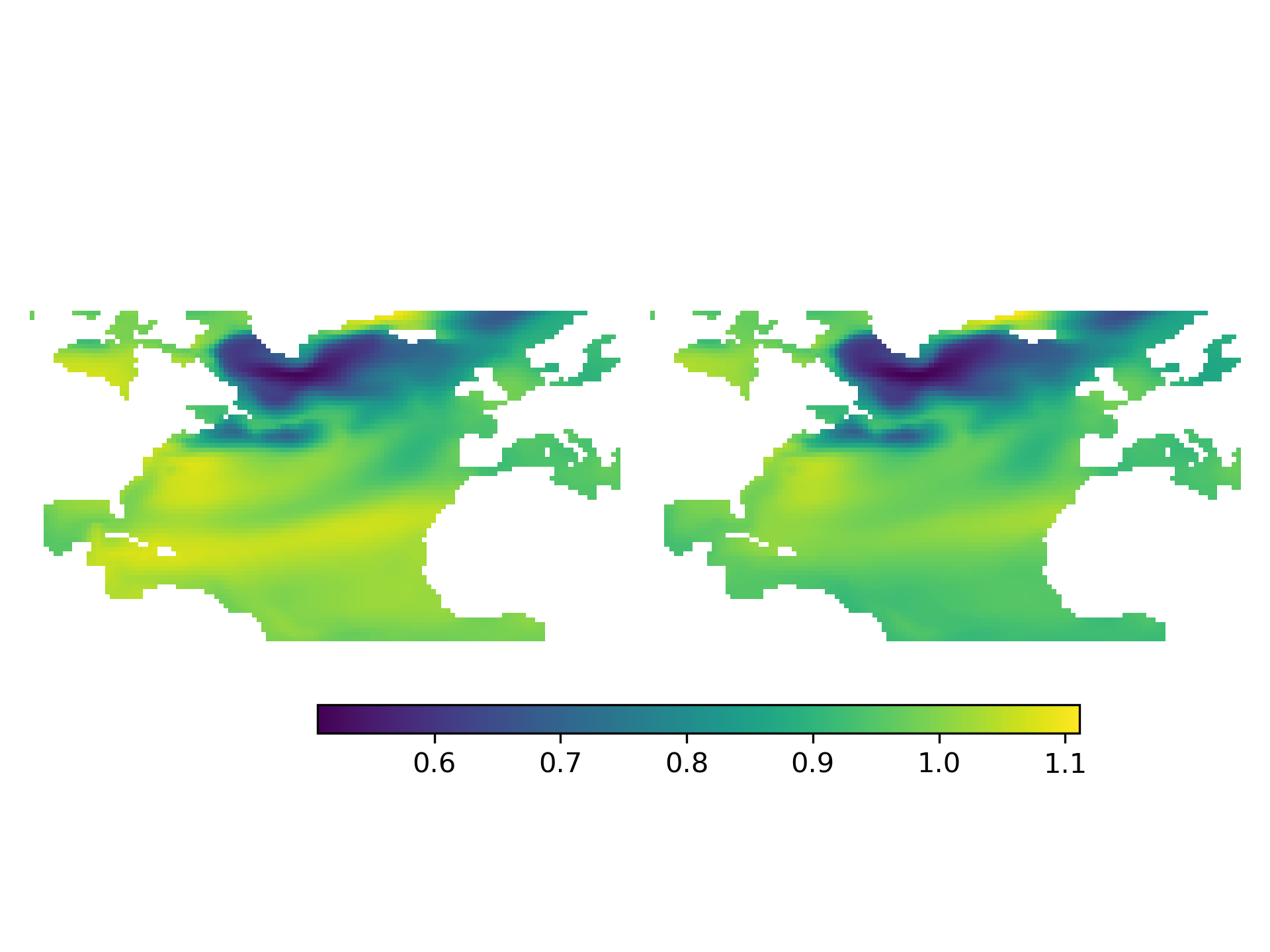
Figure 4: Spatial distribution of the normalized root mean square error at a prediction lead time of one year, averaged over ($N_{st}$=213) prediction starts. The LIM result is shown on the left and the RC result on the right. While the overall patterns of error are similar (lower errors in the sub-polar gyre, etc.), the RC methodology is seen to display consistently smaller errors (e.g., note the brighter yellow in the LIM result midway between Florida and Africa and further South).

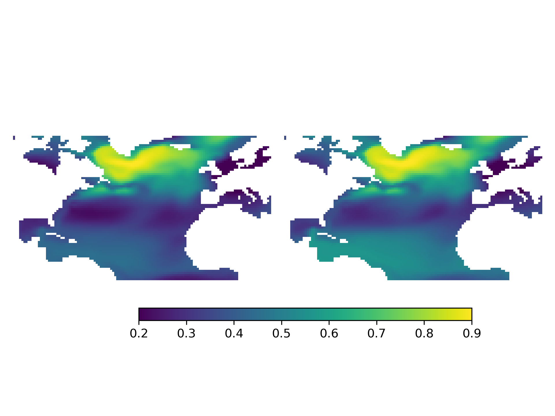
Figure 5: Anomaly correlation coefficient between the reference CESM2 SST and the LIM predictions (left) and the RC predictions (right) at the same prediction lead time of one year, computed over ($N_{st}$=213) prediction starts. Similar to the comparisons of errors in Fig. 4, while the overall patterns are again the same in the two approaches, the RC methodology displays consistently higher correlation skill (e.g., again focussing on the region midway between Florida and Africa and further South).

Figure 6: Spatially integrated skill measures are shown as a function of prediction lead time. Normalized RMSE is shown in thick lines using the left axis and anomaly correlation coefficient is shown in dot-dashed lines using the right axis. LIM results are shown in blue and RC results are shown in orange. The main plot shows results for predictions using 30 EOFs. The corresponding results for predictions using 4 EOFs is shown in the inset. All three axes in the inset have the same limits as in the main plot. The thinner blue line in the main plot is a theoretical estimate of the error in the LIM approach if the actual dynamics (that of SST in CESM2) were linear (notated as ifLinear in the legend; see (10)). The difference between the actual LIM error (thick blue line) and this theoretical estimate of error (ifLinear) is an indication of nonlinear dynamics in the data. The RC results show better skill, although not by much in this setting where training data is plentiful (480 years).

Predictions were limited to lead times $T_{pred}$ of 18 months since at that time, the NRMSE had already reached values close to 0.9 and the ACC had fallen to about 0.4 indicating the eventual approach to levels of skill achieved by climatology. In order to make the comparisons between the LIM and the RC approach statistically significant, predictions were started every ($T_{skip}$) 18 months over the testing period and then statistics were computed over such predictions (213 of them).

Figure 4 shows the spatial distribution of NRMSE at a prediction lead time of 12 months using the two methods, with the LIM result on the left and the RC result on the right. First, the overall similarity of the distribution of prediction error with the two methods indicates overall similarity in the behavior of the two methods. It also reiterates the greater predictability of the North Atlantic SST at higher latitudes, in the region of the subpolar gyre as compared to the mid and lower latitudes. Next, the smaller differences between the two panels reveals that the prediction error with the RC methodology is consistently lower than with the LIM approach.

Figure 5 shows the spatial distribution of the anomaly correlation coefficient for the two methods again at the same prediction lead time of 12 months as in Fig. 4. The comparison of the two panels again reveals overall similarity, but again with the RC predictions showing consistently higher correlation to the reference ESM results.

To be able to better compare the skill of predictions using the two methods, we next consider the spatially-averaged prediction error and correlation as a function of prediction lead time. This is shown in Fig. 6. In this figure, the LIM results (and diagnostics) are shown in blue lines where as the RC related results are shown in orange lines. The plots show NRMSE as a function of prediction lead time in heavy solid lines and uses the left axis, and ACC likewise in dot-dashed lines and uses the right axis. In addition, the thinner blue line shows the theoretical estimate of error of the LIM if the actual system were itself linear, and as given by (11). The main plot is for predictions using 30 EOFs where as the inset plot is for predictions using 4 EOFs. The inset plot uses the same limits for the horizontal axis and for each of the two vertical axes as in the main plot.

The difference between the theoretical estimate of LIM error if the actual system were linear and the actual LIM error indicates that there is indeed nonlinearity in the actual system and provides a basis for the expectation that nonlinear methods may be able to improve on the linear approach of LIM. Indeed, this expectation is seen to be realized by the simple RC model which essentially embodies a “weighted sum and nonlinearity” approach. While the improvement of predictive skill of RC over that of LIM is small, it is significant and consistent, both in terms of its variation with lead time and at different number of EOFs. The significance of this improvement is further reiterated on recalling that LIMs have been speculated to capture the bulk of the predictable signal in experiments that compare LIM predictions with predictions of full dynamical models (Newman  Sardeshmukh, 2017).

5.2 Learning from Limited Data

In the previous subsection we established the approximate similarity of the LIM approach and the RC approach, but with the RC predictions exhibiting better skill, when data is plentiful. Physically, training over such long samples of data amounts to generalizing the (18 month) response over a wide variety of situations. The dominance of linear behavior in that setting can be understood in numerous ways including statistical mechanics (fluctuation-dissipation theorem) and statistics. While it should be evident, we explicitly note that this does not mean that the system itself is linear. To wit, the commonplace recognition of the chaotic nature of climate (and weather) on the short timescale is clear evidence of the nonlinearity of the underlying dynamics. In this section, we are interested in this regime, a regime where nonlinearity has a greater role to play. The relevance of this regime to (initialized) interannual prediction (cf. CMIP) cannot be overstated.

As such, we now focus on comparing the two methods when training data is more limited: We limit the training period ($T_{tr}$) to about ten years (11.5 to 13.3 years; see below). With 800 years of data, we started the learning process every six years to have a large enough number of samples to estimate skill statistics. In particular, as in the previous section, the training period (now, of 10 years) was followed by a validation period and a testing period of equal lengths. The testing comprised of either three prediction starts over a testing period of 3.3 years (to give a 60:20:20 training:validation:test split) or just one 18 month prediction. Even as the second testing protocol places reduced emphasis on generalization error in evaluating predictive skill, it was considered for the reason that such single predictions are quite often of significant interest. We note that a new LIM model and a new RC model is learnt for each of the short (about 13 or 16.7 year) segments. As before, the best lag for each LIM was determined over the corresponding validation period, but this time only lags of 1, 2, 3, and 4 months were considered. Thereafter, the LIM state matrix was recomputed and the RC model trained (i.e., ${\mathbf{W}}_{out}$ was computed) over the combined training and validation splits (as in Sec. 5.1).

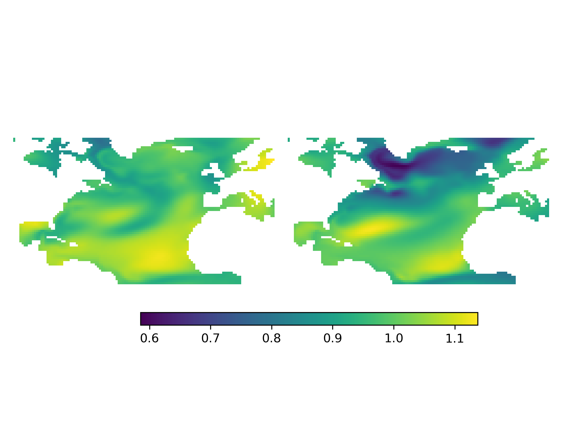
Figure 7: Comparison of NRMSE in the LIM predictions (left) and RC predictions (right), again at a lead time of one year (as in Fig. 4), but when training data is limited to about ten years. In this setting, the errors in the RC predictions are seen to be much smaller than in the LIM predictions.

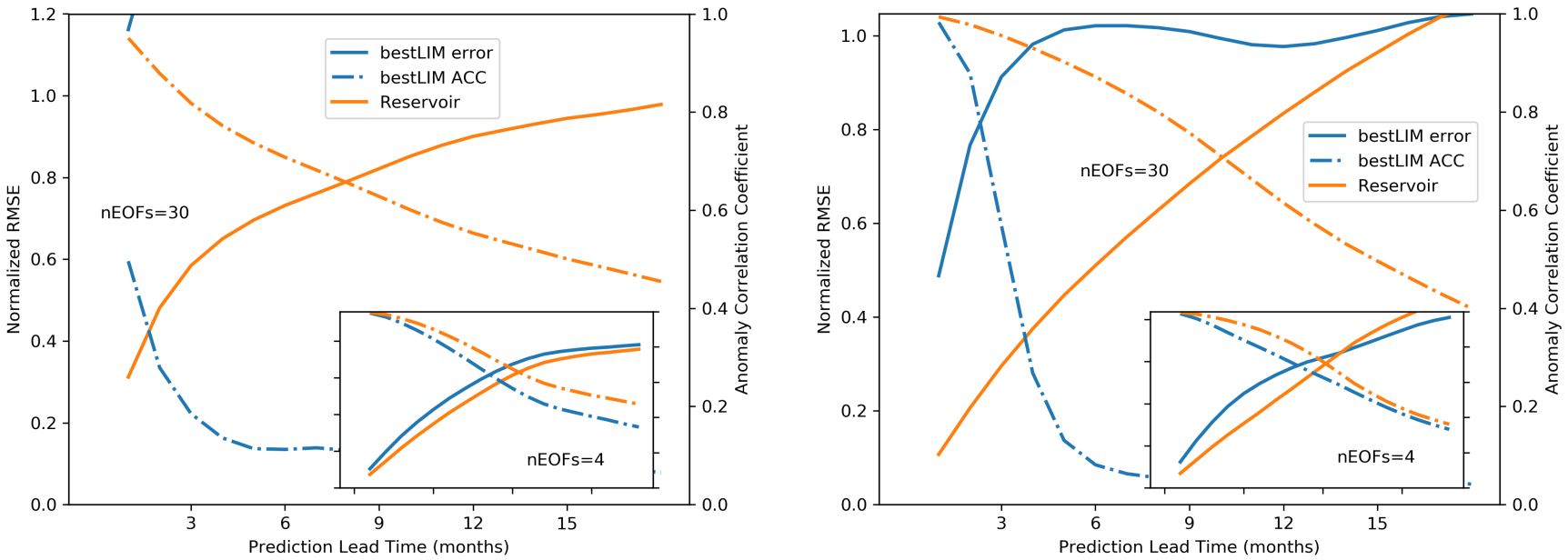
Figure 8: Like in Fig. 6, this figure compares the spatially-integrated NRMSE (left axis) and ACC (right axis) for LIM predictions (blue) and RC predictions (orange) as a function of prediction lead time when training data is limited to about 10 years. The main plots are for predictions that retain 30 EOFs whereas the inset plots are for predictions that retain only 4 EOFs. The panel on the left corresponds to testing over (at least) 20% of the data segment considered whereas the panel on the right shows results when testing is limited to predicting over a single 18 month period. The RC predictions are seen to be more skilful than the LIM predictions when 30 EOFs are retained. When only 4 EOFs are retained, their skills are comparable.

As alluded to earlier, the LIM approach can be problematic in this setting in that the learnt system can be unstable. That is, one or more of the eigenvalues of the estimated system matrix ${\mathbf{B}}$ can be positive in the limited data setting, not because of shortcomings of the estimation technique, but because the short runs of data are indeed best explained in the linear framework by a system matrix that has unstable eigenvalues. It seems that such an unstable system matrix is prone to not generalizing well and leads to problems with predictions. Rather than make ad-hoc adjustments to the procedure such as limiting the number of EOFs considered or increasing the smoothing of the data, other than noting this problem, we eliminate the LIM prediction from computing skill measures when the prediction is flagged to be unrealistic (e.g., if the predicted amplitude of any of the EOF coefficients exceeded ten times the climatological standard deviation over the prediction period). In so doing, the measures of skill for the LIM approach we present will be (artificially) inflated. For future reference, we also note that when greater than 50% of the predictions are so flagged, skill measures are considered unreliable and not used/presented (e.g., the leftmost points on the blue curves in the main panel of Fig. 9 are omitted for this reason).

Using the same format as in Fig. 4, the error using LIM and RC is shown in Fig. 7 again at a prediction lead time of 12 months (in the case where testing comprises of prediction over a single 18 month period). While the spatial distribution of errors is somewhat similar in the two methods in the sense that errors at the lower latitudes are higher, etc., RC errors are seen to be much lower than LIM errors. Similarly, the ACC for the RC predictions are seen to be much larger than for the LIM predictions (not shown). The variation of the spatially-averaged error and correlation measures as a function of prediction lead time is shown in Fig. 8 for the two testing protocols. Again, blue lines are used for LIM results and orange lines for RC results and the format is the same as in Fig. 6. These results show that when learning from short stretches of data, whereas the RC approach has much greater skill than the LIM approach when the temporal evolution of the coefficients of a large number of EOFs is being modeled (main plots in Fig. 8), their skill is comparable when only very few (four) EOFs are retained (inset plots in Fig. 8). Practically speaking, this last point is somewhat of academic interest alone. What we mean by that is: Since the skill of the RC approach with 30 EOF coefficients is not much worse than with only 4 EOF coefficients, even if the skill of the RC approach with 4 coefficients were to be worse or even much worse (than that of the LIM approach), practically one would opt for the 30 EOF coefficient prediction since it explains a much larger fraction of the variance at similar or better skill.

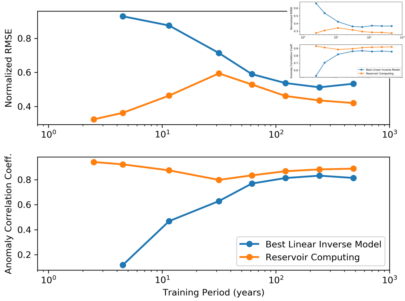
Figure 9: NRMSE and ACC of predictions of the year-1 averaged state. The main plots are for predictions retaining 30 EOF coefficients. The inset plots are for those retaining only 4. While the LIM predictions display a monotonic behavior (more data, more accurate), the RC predictions show a distinct non-monotonic behavior with a regime where accuracy improves on limiting training data.

On comparing Figs. 8 and 6, it is evident that when the RC approach outperforms the LIM approach it is largely because of the degradation of skill of the LIM approach; the skill of RC remains comparable when learning from long or short stretches of data. If $N_{y}$ (practically the same as $N_{u}$) is the number of EOFs retained, LIM in essence has to estimate $N_{y}\left(N_{y}+1\right)/2$ parameters (${\mathbf{C}}_{\tau_{0}}$ in (4)) over the training data whereas the RC approach has to estimate a much larger number of parameters that corresponds to the size of the ${\mathbf{W}}_{out}$ matrix ($\approx N_{y}\left(N_{y}+N_{r}\right)$, $N_{r}\gg N_{y}$). As such, one might expect that limited data will have a greater deleterious effect on the RC approach. Clearly, that is not the case.

At first glance, this behavior may be viewed in terms of RC being successful in fitting a better local model since it allows for nonlinearity. But, it is important to note that the better model also generalizes since otherwise we wouldn’t be seeing improvemnts in skill over the test data. In addition, we suggest that it is this behavior—the ability to perform well in situations where the number of parameters that have to be learnt are far greater than the number of samples they have to be learnt from—that the RC method shares in common with other machine and deep learning techniques and which constitutes an improvement over traditional statistical methods such as LIMs.

In order to further verify this behavior, a number of other experiments were conducted and Fig. 9 shows results from one such experiment. In this figure, the NRMSE and ACC skill measures for the prediction of the average state over the first year is plotted as a function of the training period. The main plot is for computations that retained 30 EOF coefficients whereas the inset plot is for computations that retained only four. For the case of the shortest period of training data, since greater than 50% of the predictions were flagged as unrealistic in the LIM approach, the skill measures are not indicated for that case. Perusing the plots right to left, the (more-or-less) monotonic degradation of accuracy of the LIM predictions with decreasing training data is as would be expected from a statistical perspective. The RC predictions, however, show a clear departure from this expectation with a pronounced non-monotonic behavior: skill of the RC predictions are worst at intermediate length training data (around 30 years for 30 retained EOFs and around 10 years for 4 retained EOFs). While this aspect needs to be investigated further and will be reported on in the future, we speculate that this non-monotonic behavior is related to a transition from a regime where the RC response is strongly non-linear when data is limited to a regime where the RC response is more linear when larger amounts of data are available for training.

6 Discussion

We considered a combination of settings, that included long and short learning periods and when a small number of EOFs are retained (that explained $\approx$ 50% of variance) vs. when a larger number of EOFs are retained (that explained $\approx$ 95% of variance). In almost all of these cases, the RC approach performs at least as well as the LIM approach. For simplicity, these cases can be considered as falling into two categories: one where training data is plentiful in comparison to the number of parameters to be estimated and one where data is more limited in that sense. Whereas when learning data was plentiful, the RC approach was only marginally better than the LIM approach, the RC approach performed much better than the LIM approach in settings of limited data. This difference in performance was mostly related to the strong degradation of the performance of the LIM approach. The predictive skill as a function of lead time (prediction-horizon) of the RC approach in the limited data setting was similar to that in the pentiful data setting. This needs to be investigated further. Nevertheless, the reasonable performance of the RC approach in the limited data setting is a significant and important strength. Indeed, in a more general context, it is this related ability of machine learning and deep learning models to generalize from limited data that has led to their widespread popularity (e.g., see Zhang ., 2017).

At this point, it is natural to wonder if the set of parameters used were in some sense optimal and as to what the sensitivity of the results is to changes in the parameters. As to the former, we recall that a set of parameters found to work reasonably during an initial exploration of the methodology in a particular setting was modified minimally and used to carry out all the computations in the previous section. For instance, if we consider the computation in which the RC results show a larger NRMSE at lead times of about a year and longer (inset of right panel in Fig. 8), with some searching, we were able to find new parameter settings where NRMSE of the RC predictions were everywhere lower. We avoided such a search mainly to keep the presentation simple. As to the latter other than noting that such a sensitivity analysis is beyond the scope of this article, considering the different settings in which the same set of parameters has performed reasonably, we are inclined to think that the qualitative nature of the results are likely robust, and will not change, for small but significant changes in the parameters. A limited range of (opportunistic) testing that resulted, more often than not, to not change the qualitative nature of the results presented is consistent with our expectation.

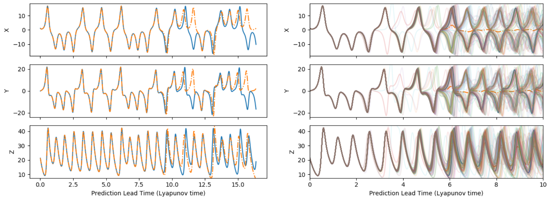
Figure 10: Reservoir computing based predictions of the Lorenz-63 system. On the left is an individual prediction whereas the full ensemble (of 128 realizations) and the ensemble-mean are shown on the right for each of the three variables (rows). The reference trajectory is shown in blue (evident in the left column, but obscured by the ensemble mean or the ensemble-members in the right column). The prediction lead time on the x-axis is non-dimensionalized in terms of the Lyapunov time (an e-folding time for error growth).

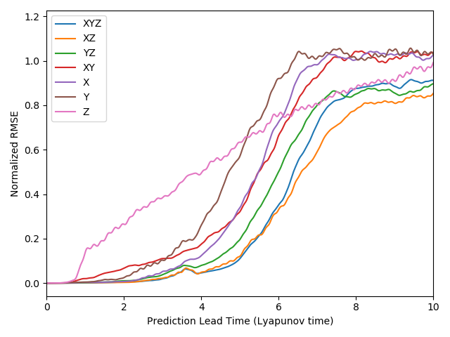
Figure 11: Normalized error as a function of prediction lead time for predictions using reservoir computing. In general (see body for details), the predictive skill diminishes when only progressively smaller parts of the system are observed and used in the RC learning and prediction procedure.

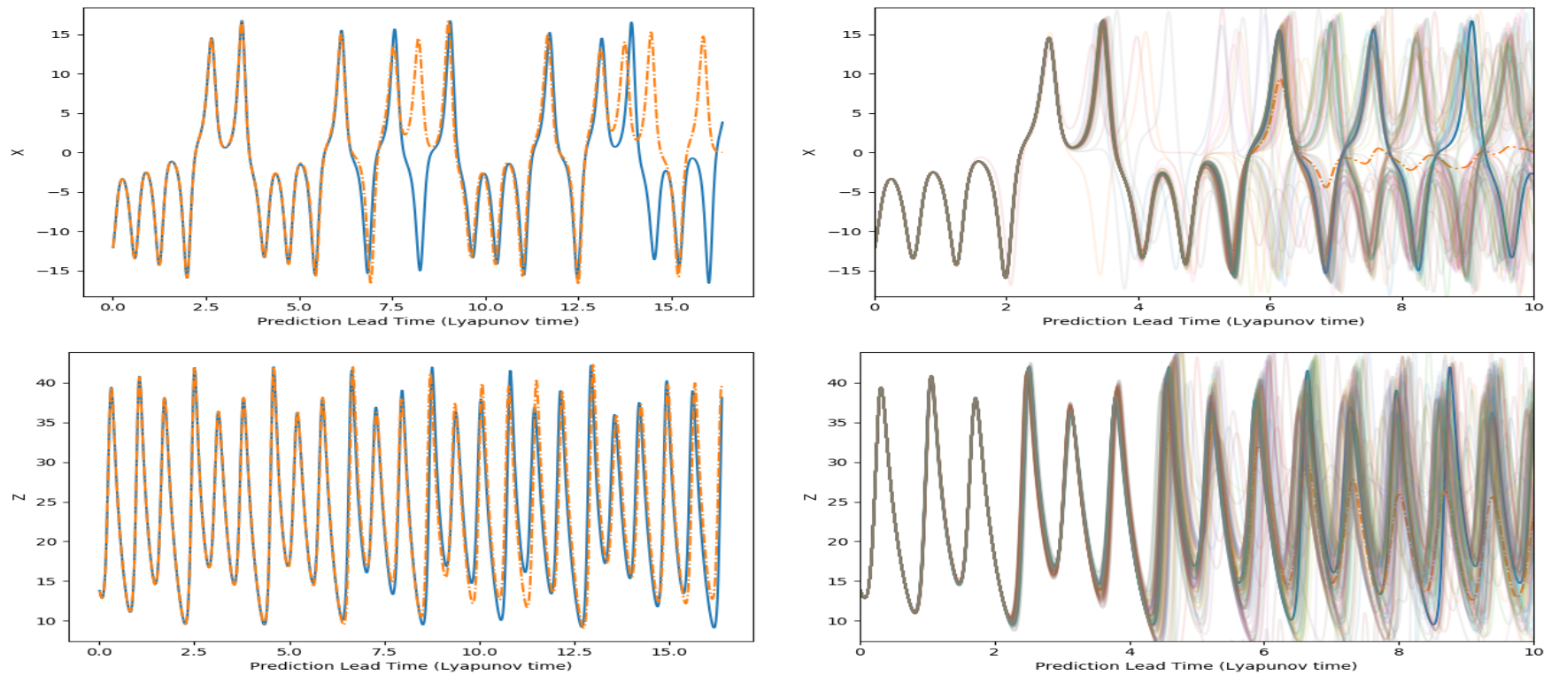
Figure 12: This figure follows the scheme in Fig. 10. Whereas Fig. 10 was for RC predictions when the system was fully observed, this figure is for RC predictions when only one of the variables was used in the RC learning and prediction procedure. Top: RC learning and prediction using only the $x$ variable in (21) (results are similar with $y$ alone). Bottom: with only $z$ variable.

Machine learning methods span a wide range of complexity and it remains an open question as to what methods are most suited for climate predictability studies in settings such as the one we consider and how far prediction skill itself can be improved. In this context, we note that preliminary results in other on-going related work where we consider other RNN architectures (Nadiga, Jiang  Farimani, 2019; Park ., 2019; Jiang ., 2019) suggest that comparable skill may be obtained using techniques with more complexity such as Convolutional Long Short Term Memory (convLSTM) architectures and that the skill of less complex architectures such as Multi-Layer Perceptrons (MLP) tends to be poor (also see Chattopadhyay ., 2020).

On the other hand, and as mentioned earlier, it might be the case that the reservoir computing paradigm that we have considered here is well suited for the problem at hand in that they have proved exceptionally good at tasks related to nonlinear system identification, prediction, and classification in the context of chaotic dynamics. To wit, Fig. 10 compares the predicted evolution of an ensemble of trajectories to a reference trajectory of the iconic Lorenz-63 system (Lorenz, 1963), hereafter referred to as L63:

$$\dot{x} = 28x-y-xz$$ (19)

$$\dot{y} = 10\left(y-x\right)$$ (20)

$$\dot{z} = -\frac{8}{3}z+xy$$ (21)

Here, the three-dimensional state vector (or a subset of it) was sampled every 0.01 time units for 100 time units after discarding an initial integration period of 10 time units and learning of the chaotic attractor and variability was achieved using the same reservoir computing approach and parameters as described in the previous section, but with a couple of modifications. The leakage parameter $\alpha_{lk}$ in the reservoir update equation (14) is now changed from the value of unity to 0.2 to approximately account for the fact that the average decorrelation time in this setting is about five times greater than that in the North Atlantic SST setting, measured in terms of the respective time intervals between data points. Furthermore, since in the previous setting we were trying to model one aspect in one region of a more complicated and more extensive multiscale system that was possibly sampled infrequently, we might expect that regularization (related to ridge regression) would be more important than in the presently setting where we are dealing with a toy three dimensional model that is well sampled. Indeed, on trying a few smaller values for the $\alpha^{2}$ parameter in (18), we find that the predictions are better at a value of 10^-6 for the $\alpha^{2}$ parameter. In other details, the data was split in a 60:40 train:test fashion, predictions were continued for 18 time units and predictions over the test section were started every 0.2 time units to allow for 110 start times. Performance measures were averaged over the 110 starts and the ensemble average of the predictions were performed over 128 realizations.

In both the panels of this figure, the x-axis corresponds to the prediction lead time non-dimensionalized in terms of the Lyapunov time ($\approx$ 0.11 time units), a characteristic time related to error doubling. The panel on the left shows a case where the RC is seen to follow the reference trajectory over as long a period as ten times the Lyapunov time. The panel on the right shows the ensemble of RC predictions for the same reference trajectory. While the ensemble mean of the RC predictions (dot dashed orange) tracks the reference trajectory till approximately 5.5 Lyapunov times, a number of the ensemble members are seen to deviate earlier. It is also interesting to note that at later times, after the ensemble mean has departed from the reference trajectory, the structure of the attractor is still seen to be well predicted. That is in the case of the Lorenz ’63 system, the RC prediction system learns and predicts the structure of the attractor well in addition to be being able to predict the exact reference trajectory over significant periods of time (many Lyapunov times). Thus, like the results of Pathak . (2018), Fig. 10 demonstrates the skill of RC, in being able to learn chaotic variability.

We conducted a few more experiments to be able to relate the good performance of the RC approach in the L63 context to the kinds of performance that we presented in the previous section in the context of predicting SST in the North Atlantic in the pre-industrial control run of the CESM2 climate model. Figure. 11 documents the results of these experiments in terms of the growth of error as a function of prediction lead time when the system is fully observed (blue lines) or only partially observed (other colors). Here, by partially observed, we mean that the learning and prediction were performed with only one or two of the three variable system (for a total of six cases—the six colors other than blue). One set of RC predictions when the system was fully observed (blue line) was considered in Fig. 10. While we prefer the use of NRMSE as a convenient diagnostic for various reasons, its usage in Fig. 11 hides the fact that when different combinations of variables are chosen for learning and prediction, the reference level of climatological variance changes in each of the experiments. It is for this reason that the error in a partial-observation experiment (e.g., the experiment labeled XZ) can show up as being less than in the fully observed system. Otherwise, a conclusion that may be drawn from these experiments is that the skill in the RC predictions decreases as fewer variables of the system are observed. That is to say, the faster loss of skill in the SST context may likewise be due to the fact that regional SST is only one small component of the, more complicated, full model climate system that is being modeled in isolation.

Plots similar to Fig. 10—the fully observed case—are shown in Fig. 12 for (one of the 110 sample predictions each) for the two cases where only the X variable is observed (top row) and only the Z variable is observed (bottom row). The case when only the Y variable is observed is similar to when only the X variable is observed and so not shown. Again, beyond times when the reference trajectory is correctly predicted, the RC predictions are seen to capture the climatological behavior reasonably. This is in spite of the fact that the dimension of the observed and modeled system is too low to even allow for chaotic behavior (cf. Poincare-Bendixon theorem, (e.g., see Guckenheimer  Holmes, 2013)). We conclude this section by noting that we are working on further improvements to the RC methodology that will permit us to use it similarly (as in the L63 setting) as a climate emulator.

7 Conclusion

Ensemble simulations are an essential tool for understanding predictability of climate. Thus, when dealing with observations of the actual climate system or with comprehensive climate models in their own right, reduced-order dynamical models play a central role by enabling simulation of large ensembles when such ensemble simulations are otherwise either not possible or are computationally expensive and resource-intensive. Furthermore such reduced order dynamical models facilitate the testing and comparison of dynamical mechanisms across models and in observational data.

While the LIM approach has proved valuable as such a reduced order modeling strategy, we have demonstrated that the nonlinear reservoir computing approach exhibits useful skill over a wider range of conditions including extending into regimes of limited data (more nonlinear) and being able to accomodate large numbers of EOF coefficients (that explain a greater fraction of the variance). While such improved predictive skill of the new approach needs to be verified in other settings, we do not see a priori reasons why this should be difficult or impossible unless of course the system itself is largely linear. Clearly, establishing predictive skill of a method is the first step towards facilitating its use in understanding issues related to predictability such as the dynamics of error growth and the structure of optimal perturbations, and we expect to report on these topics in the near future.

The difference in computational cost between the LIM approach and the RC approach is not a significant consideration in the reduced order modeling framework that we have considered: In particular, given the linear setting and the additive nature of the stochastic forcing in the LIM approach, explicit averaging over noise realizations is not required. However, the nonlinear nature of the RC approach necessitates explicit averaging over random realizations of the weights involved (but the realizations are trivially parallelizable). Apart from that, a crude estimation of the asymptotic scaling of the RC approach suggests an O($N^{2}_{\tilde{r}}T_{tr}$) scaling for the plentiful data regime and O($N^{3}_{\tilde{r}}$) in the very short training data regime, making it’s computational cost very low in the reduced dimension setting we have considered.

In addition to the previously mentioned difficulty of optimizing the design of the reservoir, the issue of interaction of randomnes of the weight matrices with other hyper-parameters needs to be better understood. For example, in certain hyper-parameter regimes, while some realizations of the random weights may give reasonable predictions, others could be unreasonable. That is to say, the ensemble can be over-dispersive. It is possible that such behavior is more common when the reservoir is operating in a regime that is close to violating the “echo state property.” Even though the latter property is controlled by parameters such as the spectral radius of the connectivity matrix, it is difficult to guarantee the property in an a priori fashion while also guaranteeing reasonable performance. A solution to this problem resides in part in tuning the system to be away from such regimes using hyper-parameter tuning. A less-attractive alternative (because it modifies the ensemble spread explicitly) is to address this issue in a posterior fashion as was done for the LIM approach in the limited data setting.

Aside from such practical considerations, at a more fundamental level, given its basis in nonlinear kernel methods, it is possible that the RC approach, will give insights into the nature of predictability that are not accessible to linear points of view, where an example of an insight provided by the LIM approach is that of non-normal finite time amplification of perturbations in an asymptotically stable system (e.g., see Penland  Sardeshmukh, 1995; Farrell  Ioannou, 2001). For example, apart from improved predictive skill, it is possible that future developments of the RC method will permit its use as a climate emulator.

References

- Abramov \BBA Majda (\APACyear2007) \APACinsertmetastarabramov2007blended{APACrefauthors}Abramov, R\BPBIV.\BCBT \BBA Majda, A\BPBIJ. \APACrefYearMonthDay2007. \BBOQ\APACrefatitleBlended response algorithms for linear fluctuation-dissipation for complex nonlinear dynamical systems Blended response algorithms for linear fluctuation-dissipation for complex nonlinear dynamical systems.\BBCQ \APACjournalVolNumPagesNonlinearity20122793. \PrintBackRefs\CurrentBib
- Adger (\APACyear2010) \APACinsertmetastaradger2010social{APACrefauthors}Adger, W\BPBIN. \APACrefYearMonthDay2010. \BBOQ\APACrefatitleSocial capital, collective action, and adaptation to climate change Social capital, collective action, and adaptation to climate change.\BBCQ \BIn \APACrefbtitleDer klimawandel Der klimawandel (\BPGS 327–345). \APACaddressPublisherSpringer. \PrintBackRefs\CurrentBib
- Alexander \BOthers. (\APACyear2008) \APACinsertmetastaralexander2008forecasting{APACrefauthors}Alexander, M\BPBIA., Matrosova, L., Penland, C., Scott, J\BPBID.\BCBL \BBA Chang, P. \APACrefYearMonthDay2008. \BBOQ\APACrefatitleForecasting Pacific SSTs: Linear inverse model predictions of the PDO Forecasting pacific ssts: Linear inverse model predictions of the pdo.\BBCQ \APACjournalVolNumPagesJournal of Climate212385–402. \PrintBackRefs\CurrentBib
- Arcomano \BOthers. (\APACyear2020) \APACinsertmetastararcomano2020machine{APACrefauthors}Arcomano, T., Szunyogh, I., Pathak, J., Wikner, A., Hunt, B\BPBIR.\BCBL \BBA Ott, E. \APACrefYearMonthDay2020. \BBOQ\APACrefatitleA Machine Learning-Based Global Atmospheric Forecast Model A machine learning-based global atmospheric forecast model.\BBCQ \APACjournalVolNumPagesGeophysical Research Letters479e2020GL087776. \PrintBackRefs\CurrentBib
- Blumenthal (\APACyear1991) \APACinsertmetastarblumenthal1991predictability{APACrefauthors}Blumenthal, M\BPBIB. \APACrefYearMonthDay1991. \BBOQ\APACrefatitlePredictability of a coupled ocean–atmosphere model Predictability of a coupled ocean–atmosphere model.\BBCQ \APACjournalVolNumPagesJournal of climate48766–784. \PrintBackRefs\CurrentBib
- Boer (\APACyear2004) \APACinsertmetastarboer2004long{APACrefauthors}Boer, G\BPBIJ. \APACrefYearMonthDay2004. \BBOQ\APACrefatitleLong time-scale potential predictability in an ensemble of coupled climate models Long time-scale potential predictability in an ensemble of coupled climate models.\BBCQ \APACjournalVolNumPagesClimate dynamics23129–44. \PrintBackRefs\CurrentBib
- Chattopadhyay \BOthers. (\APACyear2020) \APACinsertmetastarchattopadhyay2020data{APACrefauthors}Chattopadhyay, A., Hassanzadeh, P.\BCBL \BBA Subramanian, D. \APACrefYearMonthDay2020. \BBOQ\APACrefatitleData-driven predictions of a multiscale Lorenz 96 chaotic system using machine-learning methods: reservoir computing, artificial neural network, and long short-term memory network Data-driven predictions of a multiscale lorenz 96 chaotic system using machine-learning methods: reservoir computing, artificial neural network, and long short-term memory network.\BBCQ \APACjournalVolNumPagesNonlinear Processes in Geophysics273373–389. \PrintBackRefs\CurrentBib
- Collins \BOthers. (\APACyear2006) \APACinsertmetastarcollins2006interannual{APACrefauthors}Collins, M., Botzet, M., Carril, A., Drange, H., Jouzeau, A., Latif, M.\BDBLothers \APACrefYearMonthDay2006. \BBOQ\APACrefatitleInterannual to decadal climate predictability in the North Atlantic: a multimodel-ensemble study Interannual to decadal climate predictability in the north atlantic: a multimodel-ensemble study.\BBCQ \APACjournalVolNumPagesJournal of climate1971195–1203. \PrintBackRefs\CurrentBib
- Council \BOthers. (\APACyear2008) \APACinsertmetastarnational2008ecological{APACrefauthors}Council, N\BPBIR.\BCBT \BOthersPeriod. \APACrefYear2008. \APACrefbtitleEcological impacts of climate change Ecological impacts of climate change. \APACaddressPublisherNational Academies Press. \PrintBackRefs\CurrentBib
- Cybenko (\APACyear1989) \APACinsertmetastarcybenko1989approximation{APACrefauthors}Cybenko, G. \APACrefYearMonthDay1989. \BBOQ\APACrefatitleApproximation by superpositions of a sigmoidal function Approximation by superpositions of a sigmoidal function.\BBCQ \APACjournalVolNumPagesMathematics of control, signals and systems24303–314. \PrintBackRefs\CurrentBib
- Danabasoglu \BOthers. (\APACyear2020) \APACinsertmetastardanabasoglu2020community{APACrefauthors}Danabasoglu, G., Lamarque, J\BHBIF., Bacmeister, J., Bailey, D., DuVivier, A., Edwards, J.\BDBLothers \APACrefYearMonthDay2020. \BBOQ\APACrefatitleThe Community Earth System Model version 2 (CESM2) The community earth system model version 2 (cesm2).\BBCQ \APACjournalVolNumPagesJournal of Advances in Modeling Earth Systems122e2019MS001916. \PrintBackRefs\CurrentBib
- DeGennaro \BOthers. (\APACyear2019) \APACinsertmetastardegennaro2018model{APACrefauthors}DeGennaro, A\BPBIM., Urban, N\BPBIM., Nadiga, B\BPBIT.\BCBL \BBA Haut, T. \APACrefYearMonthDay2019. \BBOQ\APACrefatitleMODEL STRUCTURAL INFERENCE USING LOCAL DYNAMIC OPERATORS Model structural inference using local dynamic operators.\BBCQ \APACjournalVolNumPagesInternational Journal for Uncertainty Quantification9159–83. {APACrefURL} \urlhttp://dx.doi.org/10.1615/Int.J.UncertaintyQuantification.2019025828 {APACrefDOI} 10.1615/Int.J.UncertaintyQuantification.2019025828 \PrintBackRefs\CurrentBib
- Delworth \BBA Mann (\APACyear2000) \APACinsertmetastardelworth2000observed{APACrefauthors}Delworth, T\BPBIL.\BCBT \BBA Mann, M\BPBIE. \APACrefYearMonthDay2000. \BBOQ\APACrefatitleObserved and simulated multidecadal variability in the Northern Hemisphere Observed and simulated multidecadal variability in the northern hemisphere.\BBCQ \APACjournalVolNumPagesClimate Dynamics169661–676. \PrintBackRefs\CurrentBib
- Ehrendorfer (\APACyear1994) \APACinsertmetastarehrendorfer1994liouville{APACrefauthors}Ehrendorfer, M. \APACrefYearMonthDay1994. \BBOQ\APACrefatitleThe Liouville equation and its potential usefulness for the prediction of forecast skill. Part I: Theory The liouville equation and its potential usefulness for the prediction of forecast skill. part i: Theory.\BBCQ \APACjournalVolNumPagesMonthly Weather Review1224703–713. \PrintBackRefs\CurrentBib
- Farrell \BBA Ioannou (\APACyear2001) \APACinsertmetastarfarrell2001accurate{APACrefauthors}Farrell, B\BPBIF.\BCBT \BBA Ioannou, P\BPBIJ. \APACrefYearMonthDay2001. \BBOQ\APACrefatitleAccurate low-dimensional approximation of the linear dynamics of fluid flow Accurate low-dimensional approximation of the linear dynamics of fluid flow.\BBCQ \APACjournalVolNumPagesJournal of the atmospheric sciences58182771–2789. \PrintBackRefs\CurrentBib
- Gottwald \BBA Reich (\APACyear2020) \APACinsertmetastargottwald2020supervised{APACrefauthors}Gottwald, G\BPBIA.\BCBT \BBA Reich, S. \APACrefYearMonthDay2020. \BBOQ\APACrefatitleSupervised learning from noisy observations: Combining machine-learning techniques with data assimilation Supervised learning from noisy observations: Combining machine-learning techniques with data assimilation.\BBCQ \APACjournalVolNumPagesarXiv preprint arXiv:2007.07383. \PrintBackRefs\CurrentBib
- Grieger \BBA Latif (\APACyear1994) \APACinsertmetastargrieger1994reconstruction{APACrefauthors}Grieger, B.\BCBT \BBA Latif, M. \APACrefYearMonthDay1994. \BBOQ\APACrefatitleReconstruction of the El Niño attractor with neural networks Reconstruction of the el niño attractor with neural networks.\BBCQ \APACjournalVolNumPagesClimate Dynamics106-7267–276. \PrintBackRefs\CurrentBib
- Griffies \BBA Bryan (\APACyear1997) \APACinsertmetastargriffies1997predictability{APACrefauthors}Griffies, S\BPBIM.\BCBT \BBA Bryan, K. \APACrefYearMonthDay1997. \BBOQ\APACrefatitlePredictability of North Atlantic multidecadal climate variability Predictability of north atlantic multidecadal climate variability.\BBCQ \APACjournalVolNumPagesScience2755297181–184. \PrintBackRefs\CurrentBib
- Gritsun \BBA Branstator (\APACyear2007) \APACinsertmetastargritsun2007climate{APACrefauthors}Gritsun, A.\BCBT \BBA Branstator, G. \APACrefYearMonthDay2007. \BBOQ\APACrefatitleClimate response using a three-dimensional operator based on the fluctuation–dissipation theorem Climate response using a three-dimensional operator based on the fluctuation–dissipation theorem.\BBCQ \APACjournalVolNumPagesJournal of the atmospheric sciences6472558–2575. \PrintBackRefs\CurrentBib
- Guckenheimer \BBA Holmes (\APACyear2013) \APACinsertmetastarguckenheimer2013nonlinear{APACrefauthors}Guckenheimer, J.\BCBT \BBA Holmes, P. \APACrefYear2013. \APACrefbtitleNonlinear oscillations, dynamical systems, and bifurcations of vector fields Nonlinear oscillations, dynamical systems, and bifurcations of vector fields (\BVOL 42). \APACaddressPublisherSpringer Science & Business Media. \PrintBackRefs\CurrentBib
- Ham \BOthers. (\APACyear2019) \APACinsertmetastarham2019deep{APACrefauthors}Ham, Y\BHBIG., Kim, J\BHBIH.\BCBL \BBA Luo, J\BHBIJ. \APACrefYearMonthDay2019. \BBOQ\APACrefatitleDeep learning for multi-year ENSO forecasts Deep learning for multi-year ENSO forecasts.\BBCQ \APACjournalVolNumPagesNature5737775568–572. \PrintBackRefs\CurrentBib
- Hasselmann (\APACyear1988) \APACinsertmetastarhasselmann1988pips{APACrefauthors}Hasselmann, K. \APACrefYearMonthDay1988. \BBOQ\APACrefatitlePIPs and POPs: The reduction of complex dynamical systems using principal interaction and oscillation patterns Pips and pops: The reduction of complex dynamical systems using principal interaction and oscillation patterns.\BBCQ \APACjournalVolNumPagesJournal of Geophysical Research: Atmospheres93D911015–11021. \PrintBackRefs\CurrentBib
- Hawkins \BOthers. (\APACyear2011) \APACinsertmetastarhawkins2011evaluating{APACrefauthors}Hawkins, E., Robson, J., Sutton, R., Smith, D.\BCBL \BBA Keenlyside, N. \APACrefYearMonthDay2011. \BBOQ\APACrefatitleEvaluating the potential for statistical decadal predictions of sea surface temperatures with a perfect model approach Evaluating the potential for statistical decadal predictions of sea surface temperatures with a perfect model approach.\BBCQ \APACjournalVolNumPagesClimate dynamics3711-122495–2509. \PrintBackRefs\CurrentBib
- Hawkins \BBA Sutton (\APACyear2008) \APACinsertmetastarhawkins2008potential{APACrefauthors}Hawkins, E.\BCBT \BBA Sutton, R. \APACrefYearMonthDay2008. \BBOQ\APACrefatitlePotential predictability of rapid changes in the Atlantic meridional overturning circulation Potential predictability of rapid changes in the atlantic meridional overturning circulation.\BBCQ \APACjournalVolNumPagesGeophysical research letters3511. \PrintBackRefs\CurrentBib
- Hawkins \BBA Sutton (\APACyear2009) \APACinsertmetastarhawkins2009decadal{APACrefauthors}Hawkins, E.\BCBT \BBA Sutton, R. \APACrefYearMonthDay2009. \BBOQ\APACrefatitleDecadal predictability of the Atlantic Ocean in a coupled GCM: Forecast skill and optimal perturbations using linear inverse modeling Decadal predictability of the atlantic ocean in a coupled gcm: Forecast skill and optimal perturbations using linear inverse modeling.\BBCQ \APACjournalVolNumPagesJournal of Climate22143960–3978. \PrintBackRefs\CurrentBib
- Hsieh \BBA Tang (\APACyear1998) \APACinsertmetastarhsieh1998applying{APACrefauthors}Hsieh, W\BPBIW.\BCBT \BBA Tang, B. \APACrefYearMonthDay1998. \BBOQ\APACrefatitleApplying neural network models to prediction and data analysis in meteorology and oceanography Applying neural network models to prediction and data analysis in meteorology and oceanography.\BBCQ \APACjournalVolNumPagesBulletin of the American Meteorological Society7991855–1870. \PrintBackRefs\CurrentBib
- Jaeger (\APACyear2001) \APACinsertmetastarjaeger2001echo{APACrefauthors}Jaeger, H. \APACrefYearMonthDay2001. \BBOQ\APACrefatitleThe “echo state” approach to analysing and training recurrent neural networks-with an erratum note The “echo state” approach to analysing and training recurrent neural networks-with an erratum note.\BBCQ \APACjournalVolNumPagesBonn, Germany: German National Research Center for Information Technology GMD Technical Report1483413. \PrintBackRefs\CurrentBib
- Jaeger \BBA Haas (\APACyear2004) \APACinsertmetastarjaeger2004harnessing{APACrefauthors}Jaeger, H.\BCBT \BBA Haas, H. \APACrefYearMonthDay2004. \BBOQ\APACrefatitleHarnessing nonlinearity: Predicting chaotic systems and saving energy in wireless communication Harnessing nonlinearity: Predicting chaotic systems and saving energy in wireless communication.\BBCQ \APACjournalVolNumPagesscience304566778–80. \PrintBackRefs\CurrentBib
- Jaeger \BOthers. (\APACyear2007) \APACinsertmetastarjaeger2007special{APACrefauthors}Jaeger, H., Maass, W.\BCBL \BBA Principe, J. \APACrefYearMonthDay2007. \BBOQ\APACrefatitleSpecial issue on echo state networks and liquid state machines. Special issue on echo state networks and liquid state machines.\BBCQ \PrintBackRefs\CurrentBib
- Jiang \BOthers. (\APACyear2019) \APACinsertmetastarjiang2019interannual{APACrefauthors}Jiang, C., Nadiga, B\BPBIT.\BCBL \BBA Farimani, A. \APACrefYearMonthDay2019. \BBOQ\APACrefatitleInterannual Variability of Climate using Deep Learning Interannual variability of climate using deep learning.\BBCQ \APACjournalVolNumPagesin Proceedings of the 9th International Workshop on Climate Informatics: CI 2019, Brajard, J., Charantonis, A., Chen, C., & Runge, J. (Eds.). (No. NCAR/TN-561+PROC). doi:10.5065/y82j-f154. \PrintBackRefs\CurrentBib
- Kharin \BOthers. (\APACyear2012) \APACinsertmetastarkharin2012statistical{APACrefauthors}Kharin, V., Boer, G., Merryfield, W., Scinocca, J.\BCBL \BBA Lee, W\BHBIS. \APACrefYearMonthDay2012. \BBOQ\APACrefatitleStatistical adjustment of decadal predictions in a changing climate Statistical adjustment of decadal predictions in a changing climate.\BBCQ \APACjournalVolNumPagesGeophysical Research Letters3919. \PrintBackRefs\CurrentBib
- Kim \BOthers. (\APACyear2012) \APACinsertmetastarkim2012evaluation{APACrefauthors}Kim, H\BHBIM., Webster, P\BPBIJ.\BCBL \BBA Curry, J\BPBIA. \APACrefYearMonthDay2012. \BBOQ\APACrefatitleEvaluation of short-term climate change prediction in multi-model CMIP5 decadal hindcasts Evaluation of short-term climate change prediction in multi-model cmip5 decadal hindcasts.\BBCQ \APACjournalVolNumPagesGeophysical Research Letters3910. \PrintBackRefs\CurrentBib
- Kondrashov \BOthers. (\APACyear2018) \APACinsertmetastarkondrashov2018data{APACrefauthors}Kondrashov, D., Chekroun, M\BPBID., Yuan, X.\BCBL \BBA Ghil, M. \APACrefYearMonthDay2018. \BBOQ\APACrefatitleData-adaptive harmonic decomposition and stochastic modeling of Arctic sea ice Data-adaptive harmonic decomposition and stochastic modeling of arctic sea ice.\BBCQ \BIn \APACrefbtitleAdvances in Nonlinear Geosciences Advances in nonlinear geosciences (\BPGS 179–205). \APACaddressPublisherSpringer. \PrintBackRefs\CurrentBib
- Kondrashov \BOthers. (\APACyear2005) \APACinsertmetastarkondrashov2005hierarchy{APACrefauthors}Kondrashov, D., Kravtsov, S., Robertson, A\BPBIW.\BCBL \BBA Ghil, M. \APACrefYearMonthDay2005. \BBOQ\APACrefatitleA hierarchy of data-based ENSO models A hierarchy of data-based ENSO models.\BBCQ \APACjournalVolNumPagesJournal of climate18214425–4444. \PrintBackRefs\CurrentBib
- Leith (\APACyear1975) \APACinsertmetastarleith1975climate{APACrefauthors}Leith, C. \APACrefYearMonthDay1975. \BBOQ\APACrefatitleClimate response and fluctuation dissipation Climate response and fluctuation dissipation.\BBCQ \APACjournalVolNumPagesJournal of the Atmospheric Sciences32102022–2026. \PrintBackRefs\CurrentBib
- Lorenz (\APACyear1963) \APACinsertmetastarlorenz1963deterministic{APACrefauthors}Lorenz, E\BPBIN. \APACrefYearMonthDay1963. \BBOQ\APACrefatitleDeterministic nonperiodic flow Deterministic nonperiodic flow.\BBCQ \APACjournalVolNumPagesJournal of the atmospheric sciences202130–141. \PrintBackRefs\CurrentBib
- Lorenz (\APACyear1965) \APACinsertmetastarlorenz1965study{APACrefauthors}Lorenz, E\BPBIN. \APACrefYearMonthDay1965. \BBOQ\APACrefatitleA study of the predictability of a 28-variable atmospheric model A study of the predictability of a 28-variable atmospheric model.\BBCQ \APACjournalVolNumPagesTellus173321–333. \PrintBackRefs\CurrentBib
- Lorenz (\APACyear1969) \APACinsertmetastarlorenz1969three{APACrefauthors}Lorenz, E\BPBIN. \APACrefYearMonthDay1969. \BBOQ\APACrefatitleThree approaches to atmospheric predictability Three approaches to atmospheric predictability.\BBCQ \APACjournalVolNumPagesBull. Amer. Meteor. Soc503454349. \PrintBackRefs\CurrentBib
- Lorenz (\APACyear1975) \APACinsertmetastarlorenz1975predictability{APACrefauthors}Lorenz, E\BPBIN. \APACrefYearMonthDay1975. \BBOQ\APACrefatitleClimate predictability Climate predictability.\BBCQ \BIn \APACrefbtitleThe physical basis of climate modeling. GARP Publication Series, WMO The physical basis of climate modeling. garp publication series, WMO (\BVOL 16, \BPGS 132–136). \PrintBackRefs\CurrentBib
- Lukoševičius \BBA Jaeger (\APACyear2009) \APACinsertmetastarlukovsevivcius2009reservoir{APACrefauthors}Lukoševičius, M.\BCBT \BBA Jaeger, H. \APACrefYearMonthDay2009. \BBOQ\APACrefatitleReservoir computing approaches to recurrent neural network training Reservoir computing approaches to recurrent neural network training.\BBCQ \APACjournalVolNumPagesComputer Science Review33127–149. \PrintBackRefs\CurrentBib
- Maass \BOthers. (\APACyear2002) \APACinsertmetastarmaass2002real{APACrefauthors}Maass, W., Natschläger, T.\BCBL \BBA Markram, H. \APACrefYearMonthDay2002. \BBOQ\APACrefatitleReal-time computing without stable states: A new framework for neural computation based on perturbations Real-time computing without stable states: A new framework for neural computation based on perturbations.\BBCQ \APACjournalVolNumPagesNeural computation14112531–2560. \PrintBackRefs\CurrentBib
- Meehl \BOthers. (\APACyear2014) \APACinsertmetastarmeehl2014decadal{APACrefauthors}Meehl, G\BPBIA., Goddard, L., Boer, G., Burgman, R., Branstator, G., Cassou, C.\BDBLothers \APACrefYearMonthDay2014. \BBOQ\APACrefatitleDecadal climate prediction: an update from the trenches Decadal climate prediction: an update from the trenches.\BBCQ \APACjournalVolNumPagesBulletin of the American Meteorological Society952243–267. \PrintBackRefs\CurrentBib
- Meehl \BOthers. (\APACyear2009) \APACinsertmetastarmeehl2009decadal{APACrefauthors}Meehl, G\BPBIA., Goddard, L., Murphy, J., Stouffer, R\BPBIJ., Boer, G., Danabasoglu, G.\BDBLothers \APACrefYearMonthDay2009. \BBOQ\APACrefatitleDecadal prediction: can it be skillful? Decadal prediction: can it be skillful?\BBCQ \APACjournalVolNumPagesBulletin of the American Meteorological Society90101467–1486. \PrintBackRefs\CurrentBib
- Mills (\APACyear2005) \APACinsertmetastarmills2005insurance{APACrefauthors}Mills, E. \APACrefYearMonthDay2005. \BBOQ\APACrefatitleInsurance in a climate of change Insurance in a climate of change.\BBCQ \APACjournalVolNumPagesScience30957371040–1044. \PrintBackRefs\CurrentBib
- Nadiga, Jiang\BCBL \BBA Farimani (\APACyear2019) \APACinsertmetastarnadiga2019predicting{APACrefauthors}Nadiga, B\BPBIT., Jiang, C.\BCBL \BBA Farimani, A. \APACrefYearMonthDay2019. \BBOQ\APACrefatitlePredicting interannual variability of climate using deep learning Predicting interannual variability of climate using deep learning.\BBCQ \APACjournalVolNumPagesAPSG20–007. \PrintBackRefs\CurrentBib
- Nadiga, Verma\BCBL \BOthers. (\APACyear2019) \APACinsertmetastarnadiga2019enhancing{APACrefauthors}Nadiga, B\BPBIT., Verma, T., Weijer, W.\BCBL \BBA Urban, N\BPBIM. \APACrefYearMonthDay2019. \BBOQ\APACrefatitleEnhancing skill of initialized decadal predictions using a dynamic model of drift Enhancing skill of initialized decadal predictions using a dynamic model of drift.\BBCQ \APACjournalVolNumPagesGeophysical Research Letters46169991–9999. \PrintBackRefs\CurrentBib
- Newman (\APACyear2007) \APACinsertmetastarnewman2007interannual{APACrefauthors}Newman, M. \APACrefYearMonthDay2007. \BBOQ\APACrefatitleInterannual to decadal predictability of tropical and North Pacific sea surface temperatures Interannual to decadal predictability of tropical and north pacific sea surface temperatures.\BBCQ \APACjournalVolNumPagesJournal of climate20112333–2356. \PrintBackRefs\CurrentBib
- Newman \BBA Sardeshmukh (\APACyear2017) \APACinsertmetastarnewman2017we{APACrefauthors}Newman, M.\BCBT \BBA Sardeshmukh, P\BPBID. \APACrefYearMonthDay2017. \BBOQ\APACrefatitleAre we near the predictability limit of tropical Indo-Pacific sea surface temperatures? Are we near the predictability limit of tropical indo-pacific sea surface temperatures?\BBCQ \APACjournalVolNumPagesGeophysical Research Letters44168520–8529. \PrintBackRefs\CurrentBib
- Park \BOthers. (\APACyear2019) \APACinsertmetastarparkmachine{APACrefauthors}Park, J\BPBIH., Yoo, S.\BCBL \BBA Nadiga, B\BPBIT. \APACrefYearMonthDay2019. \BBOQ\APACrefatitleMachine learning climate variability Machine learning climate variability.\BBCQ \APACjournalVolNumPagesNeurIPS 2019 workshop on Machine Learning and the Physical Sciences, \urlhttps://ml4physicalsciences.github.io/files/NeurIPS_ML4PS_2019_84.pdf. \PrintBackRefs\CurrentBib
- Pathak \BOthers. (\APACyear2018) \APACinsertmetastarpathak2018model{APACrefauthors}Pathak, J., Hunt, B., Girvan, M., Lu, Z.\BCBL \BBA Ott, E. \APACrefYearMonthDay2018. \BBOQ\APACrefatitleModel-free prediction of large spatiotemporally chaotic systems from data: A reservoir computing approach Model-free prediction of large spatiotemporally chaotic systems from data: A reservoir computing approach.\BBCQ \APACjournalVolNumPagesPhysical review letters1202024102. \PrintBackRefs\CurrentBib
- Penland (\APACyear1989) \APACinsertmetastarpenland1989random{APACrefauthors}Penland, C. \APACrefYearMonthDay1989. \BBOQ\APACrefatitleRandom forcing and forecasting using principal oscillation pattern analysis Random forcing and forecasting using principal oscillation pattern analysis.\BBCQ \APACjournalVolNumPagesMonthly Weather Review117102165–2185. \PrintBackRefs\CurrentBib
- Penland \BBA Magorian (\APACyear1993) \APACinsertmetastarpenland1993prediction{APACrefauthors}Penland, C.\BCBT \BBA Magorian, T. \APACrefYearMonthDay1993. \BBOQ\APACrefatitlePrediction of Niño 3 sea surface temperatures using linear inverse modeling Prediction of niño 3 sea surface temperatures using linear inverse modeling.\BBCQ \APACjournalVolNumPagesJournal of Climate661067–1076. \PrintBackRefs\CurrentBib
- Penland \BBA Sardeshmukh (\APACyear1995) \APACinsertmetastarpenland1995optimal{APACrefauthors}Penland, C.\BCBT \BBA Sardeshmukh, P\BPBID. \APACrefYearMonthDay1995. \BBOQ\APACrefatitleThe optimal growth of tropical sea surface temperature anomalies The optimal growth of tropical sea surface temperature anomalies.\BBCQ \APACjournalVolNumPagesJournal of climate881999–2024. \PrintBackRefs\CurrentBib
- Pohlmann \BOthers. (\APACyear2004) \APACinsertmetastarpohlmann2004estimating{APACrefauthors}Pohlmann, H., Botzet, M., Latif, M., Roesch, A., Wild, M.\BCBL \BBA Tschuck, P. \APACrefYearMonthDay2004. \BBOQ\APACrefatitleEstimating the decadal predictability of a coupled AOGCM Estimating the decadal predictability of a coupled aogcm.\BBCQ \APACjournalVolNumPagesJournal of Climate17224463–4472. \PrintBackRefs\CurrentBib
- Rahimi \BBA Recht (\APACyear2008) \APACinsertmetastarrahimi2008random{APACrefauthors}Rahimi, A.\BCBT \BBA Recht, B. \APACrefYearMonthDay2008. \BBOQ\APACrefatitleRandom features for large-scale kernel machines Random features for large-scale kernel machines.\BBCQ \BIn \APACrefbtitleAdvances in neural information processing systems Advances in neural information processing systems (\BPGS 1177–1184). \PrintBackRefs\CurrentBib
- Sanchez-Gomez \BOthers. (\APACyear2016) \APACinsertmetastarsanchez2016drift{APACrefauthors}Sanchez-Gomez, E., Cassou, C., Ruprich-Robert, Y., Fernandez, E.\BCBL \BBA Terray, L. \APACrefYearMonthDay2016. \BBOQ\APACrefatitleDrift dynamics in a coupled model initialized for decadal forecasts Drift dynamics in a coupled model initialized for decadal forecasts.\BBCQ \APACjournalVolNumPagesClimate Dynamics465-61819–1840. \PrintBackRefs\CurrentBib
- Scher \BBA Messori (\APACyear2019) \APACinsertmetastarscher2019weather{APACrefauthors}Scher, S.\BCBT \BBA Messori, G. \APACrefYearMonthDay2019. \BBOQ\APACrefatitleWeather and climate forecasting with neural networks: using general circulation models (GCMs) with different complexity as a study ground Weather and climate forecasting with neural networks: using general circulation models (gcms) with different complexity as a study ground.\BBCQ \APACjournalVolNumPagesGeoscientific Model Development1272797–2809. \PrintBackRefs\CurrentBib
- Sévellec \BOthers. (\APACyear2008) \APACinsertmetastarsevellec2008optimal{APACrefauthors}Sévellec, F., Huck, T., Ben Jelloul, M., Grima, N., Vialard, J.\BCBL \BBA Weaver, A. \APACrefYearMonthDay2008. \BBOQ\APACrefatitleOptimal surface salinity perturbations of the meridional overturning and heat transport in a global ocean general circulation model Optimal surface salinity perturbations of the meridional overturning and heat transport in a global ocean general circulation model.\BBCQ \APACjournalVolNumPagesJournal of Physical Oceanography38122739–2754. \PrintBackRefs\CurrentBib
- Stocker \BOthers. (\APACyear2013) \APACinsertmetastarstocker2013climate{APACrefauthors}Stocker, T\BPBIF., Qin, D., Plattner, G\BHBIK., Tignor, M., Allen, S\BPBIK., Boschung, J.\BDBLothers \APACrefYearMonthDay2013. \BBOQ\APACrefatitleClimate change 2013: The physical science basis Climate change 2013: The physical science basis.\BBCQ \APACjournalVolNumPagesContribution of working group I to the fifth assessment report of the intergovernmental panel on climate change1535. \PrintBackRefs\CurrentBib
- Tang \BOthers. (\APACyear2000) \APACinsertmetastartang2000skill{APACrefauthors}Tang, B., Hsieh, W\BPBIW., Monahan, A\BPBIH.\BCBL \BBA Tangang, F\BPBIT. \APACrefYearMonthDay2000. \BBOQ\APACrefatitleSkill comparisons between neural networks and canonical correlation analysis in predicting the equatorial Pacific sea surface temperatures Skill comparisons between neural networks and canonical correlation analysis in predicting the equatorial pacific sea surface temperatures.\BBCQ \APACjournalVolNumPagesJournal of Climate131287–293. \PrintBackRefs\CurrentBib
- Timmermann \BOthers. (\APACyear2001) \APACinsertmetastartimmermann2001empirical{APACrefauthors}Timmermann, A., Voss, H.\BCBL \BBA Pasmanter, R. \APACrefYearMonthDay2001. \BBOQ\APACrefatitleEmpirical dynamical system modeling of ENSO using nonlinear inverse techniques Empirical dynamical system modeling of ENSO using nonlinear inverse techniques.\BBCQ \APACjournalVolNumPagesJournal of physical oceanography3161579–1598. \PrintBackRefs\CurrentBib
- Tu \BOthers. (\APACyear2014) \APACinsertmetastartu2014dynamic{APACrefauthors}Tu, J\BPBIH., Rowley, C\BPBIW., Luchtenburg, D\BPBIM., Brunton, S\BPBIL.\BCBL \BBA Kutz, J\BPBIN. \APACrefYearMonthDay2014. \BBOQ\APACrefatitleOn dynamic mode decomposition: Theory and applications On dynamic mode decomposition: Theory and applications.\BBCQ \APACjournalVolNumPagesJournal of Computational Dynamics12391–421. \PrintBackRefs\CurrentBib
- Von Storch \BBA Zwiers (\APACyear2001) \APACinsertmetastarvon2001statistical{APACrefauthors}Von Storch, H.\BCBT \BBA Zwiers, F\BPBIW. \APACrefYear2001. \APACrefbtitleStatistical analysis in climate research Statistical analysis in climate research. \APACaddressPublisherCambridge university press. \PrintBackRefs\CurrentBib
- Weyn \BOthers. (\APACyear2019) \APACinsertmetastarweyn2019can{APACrefauthors}Weyn, J\BPBIA., Durran, D\BPBIR.\BCBL \BBA Caruana, R. \APACrefYearMonthDay2019. \BBOQ\APACrefatitleCan machines learn to predict weather? Using deep learning to predict gridded 500-hPa geopotential height from historical weather data Can machines learn to predict weather? using deep learning to predict gridded 500-hpa geopotential height from historical weather data.\BBCQ \APACjournalVolNumPagesJournal of Advances in Modeling Earth Systems1182680–2693. \PrintBackRefs\CurrentBib
- Weyn \BOthers. (\APACyear2020) \APACinsertmetastarweyn2020improving{APACrefauthors}Weyn, J\BPBIA., Durran, D\BPBIR.\BCBL \BBA Caruana, R. \APACrefYearMonthDay2020. \BBOQ\APACrefatitleImproving data-driven global weather prediction using deep convolutional neural networks on a cubed sphere Improving data-driven global weather prediction using deep convolutional neural networks on a cubed sphere.\BBCQ \APACjournalVolNumPagesarXiv preprint arXiv:2003.11927. \PrintBackRefs\CurrentBib
- Wilbanks \BBA Fernandez (\APACyear2014) \APACinsertmetastarwilbanks2014climate{APACrefauthors}Wilbanks, T\BPBIJ.\BCBT \BBA Fernandez, S. \APACrefYear2014. \APACrefbtitleClimate change and infrastructure, urban systems, and vulnerabilities: Technical report for the US Department of Energy in support of the national climate assessment Climate change and infrastructure, urban systems, and vulnerabilities: Technical report for the us department of energy in support of the national climate assessment. \APACaddressPublisherIsland Press. \PrintBackRefs\CurrentBib
- Zhang \BOthers. (\APACyear2017) \APACinsertmetastarzhang2017understanding{APACrefauthors}Zhang, C., Bengio, S., Hardt, M., Recht, B.\BCBL \BBA Vinyals, O. \APACrefYearMonthDay2017. \APACrefbtitleUnderstanding deep learning requires rethinking generalization. Understanding deep learning requires rethinking generalization. \PrintBackRefs\CurrentBib