Piecewise linear regression and classification

Abstract

This paper proposes a method for solving multivariate regression and classification problems using piecewise linear predictors over a polyhedral partition of the feature space. The resulting algorithm that we call PARC (Piecewise Affine Regression and Classification) alternates between ($i$) solving ridge regression problems for numeric targets, softmax regression problems for categorical targets, and either softmax regression or cluster centroid computation for piecewise linear separation, and ($ii$) assigning the training points to different clusters on the basis of a criterion that balances prediction accuracy and piecewise-linear separability. We prove that PARC is a block-coordinate descent algorithm that optimizes a suitably constructed objective function, and that it converges in a finite number of steps to a local minimum of that function. The accuracy of the algorithm is extensively tested numerically on synthetic and real-world datasets, showing that the approach provides an extension of linear regression/classification that is particularly useful when the obtained predictor is used as part of an optimization model. A Python implementation of the algorithm described in this paper is available at http://cse.lab.imtlucca.it/~bemporad/parc.

Keywords: Multivariate regression, multi-category classification, piecewise linear functions, softmax regression, mixed-integer programming

1 Introduction

Several methods exist for solving supervised learning problems of regression and classification (Hastie et al., 2009; Bishop, 2006). The main goal is to estimate a model of the data generation process to predict at best the target value corresponding to a combination of features not seen before. However, not all methods are suitable to optimize on top of the estimated model, i.e., to solve a mathematical programming problem that contains the estimated model as part of the constraints and/or the objective function. For example, to find the best combination of features providing a desired target, possibly under constraints on the features one can choose. In this case, the model is used as a surrogate of the underlying (and unknown) features-to-target mapping to formulate the decision problem. Applications range from derivative-free black-box optimization (Kushner, 1964; Jones, 2001; Brochu et al., 2010; Bemporad, 2020; Bemporad and Piga, 2021), to engineering design (Queipo et al., 2005), and control engineering, in particular model predictive control (Camacho and Bordons, 1999; Mayne et al., 2018; Borrelli et al., 2017), where actuation commands are decided in real-time by a numerical optimization algorithm based on a dynamical model of the controlled process that is learned from data (Ljung, 1999; Schoukens and Ljung, 2019), see for instance the approach proposed recently in (Masti and Bemporad, 2020).

When optimizing over a learned model is a goal, a clear tradeoff exists between the accuracy of the model on test data and the complexity of the model, which ultimately determines the complexity of the mathematical programming problem resulting from using the model. On one extreme, we have linear regression models, which are very simple to represent as linear relations among optimization variables but have limited expressiveness. On the other extreme, random forests and other ensemble methods, k-nearest neighbors, kernel support vector machines, and other methods, can capture the underlying model very accurately but are difficult to encode in an optimization problem. Neural networks and Gaussian processes can be a good compromise between the compactness of the model and the representation of the feature-to-target relation, but are nonlinear models leading to nonconvex optimization problems that are possibly difficult to solve to global optimality.

In this paper, we advocate the use of piecewise linear (PWL) models as a good tradeoff between their simplicity, due to the linearity of the model on polyhedral regions of the feature-vector space, and expressiveness, due to the good approximation properties of piecewise linear functions (Breiman, 1993; Lin and Unbehauen, 1992; Chua and Deng, 1988; Julián et al., 2000; Bemporad et al., 2011). We refer to such models with the more appropriate, although less common, term piecewise affine (PWA), to highlight the presence of an intercept in each submodel. PWA models can be easily encoded into optimization problems by using mixed-integer linear inequalities (Bemporad and Morari, 1999), and hence optimize over them to reach a global minimum by using mixed-integer programming (Lodi, 2010), for which excellent public domain and commercial packages exist.

Many classical machine learning methods have an underlying PWA structure: ridge classification, logistic (and more generally softmax) regression, hinging hyperplanes (Breiman, 1993), and neural networks with ReLU activation functions, they all require evaluating the maximum of linear functions to predict target values; the predictor associated with a decision tree is a piecewise constant (PWC) function over a partition of the feature-vector space in boxes; $k$-nearest neighbor classifiers can be also expressed as PWC functions over polyhedral partitions (the comparison of squared Euclidean norms $\|x-x_{i}\|_{2}^{2}\leq\|x-x_{j}\|_{2}^{2}$ used to determine the nearest neighbors of $x$ is equivalent to the linear relation $2(x_{j}-x_{i})^{\prime}x\leq\|x_{j}\|_{2}^{2}-\|x_{i}\|_{2}^{2}$), although the number of polyhedra largely grows with the number of training samples.

Different piecewise affine regression methods have been proposed in the system identification literature for getting switching linear dynamical models from data (Ferrari-Trecate et al., 2003; Roll et al., 2004; Bemporad et al., 2005; Nakada et al., 2005; Hartmann et al., 2015). See also the survey paper (Paoletti et al., 2007) and the recursive PWA regression algorithms proposed in (Bako et al., 2011; Breschi et al., 2016). Most of such methods identify a prescribed number of linear models and associate one of them to each training datapoint, therefore determining a clustering of the data. As a last step, a multicategory discrimination problem is solved to determine a function that piecewise-linearly separates the clusters (Bennett and Mangasarian, 1994). For instance, the approach of Nakada et al. (2005) consists of first clustering the feature+target vectors by using a Gaussian mixture model, then use support vector classification to separate the feature-vector space. In (Ferrari-Trecate et al., 2003), the authors propose instead to cluster the vectors whose entries are the coefficients of local linear models, one model per datapoint, then piecewise-linearly separate the clusters. In (Breschi et al., 2016), $K$ recursive least-squares problems for regression are run in parallel to cluster data in on-line fashion, based on both quality of fit obtained by each linear model and proximity to the current centroids of the clusters, and finally the obtained clusters are separated by a PWL function.

1.1 Contribution

This paper proposes a general supervised learning method for regression and/or classification of multiple targets that results in a PWA predictor over a single PWA partition of the feature space in $K$ polyhedral cells. In each polyhedron, the predictor is either affine (for numeric targets) or given by the max of affine functions, i.e., convex piecewise affine (for categorical targets). Our goal is to obtain an overall predictor that admits a simple encoding with binary and real variables, to be able to solve optimization problems involving the prediction function via mixed-integer linear or quadratic programming. The number $K$ of linear predictors is therefore limited by the tolerated complexity of the resulting mixed-integer encoding of the PWA predictor.

Rather than first clustering the training data and fitting $K$ different linear predictors, and then finding a PWL separation function to get the PWA partition, we simultaneously cluster, PWL-separate, and fit by solving a block-coordinate descent problem, similarly to the K-means algorithm (Lloyd, 1957), where we alternate between fitting models/separating clusters and reassigning training data to clusters. We call the algorithm PARC (Piecewise Affine Regression and Classification) and show that it converges in a finite number of iterations by showing that the sum of the loss functions associated with regression, classification, piecewise linear separation errors decreases at each iteration. PWL separation is obtained by solving softmax regression problems or, as a simpler alternative, by taking the Voronoi partition induced by the cluster centroids.

We test the PARC algorithm on different synthetic and real-world datasets. After showing that PARC can reconstruct an underlying PWA function from its samples, we investigate the effect of $K$ in reconstructing a nonlinear function, also showing how to optimize with respect to the feature vector so that the corresponding target is as close as possible to a given reference value. Then we test PARC on many real-world datasets proposed for regression and classification, comparing its performance to alternative regression and classification techniques that admit a mixed-integer encoding of the predictor of similar complexity, such as simple neural networks based on ReLU activation functions and small decision trees.

A Python implementation of the PARC algorithm is available at http://cse.lab.imtlucca.it/~bemporad/parc.

1.2 Outline

After formulating the multivariate PWL regression and classification problem in Section 2, we describe the proposed PARC algorithm and prove its convergence properties in Section 3. In Section 4 we define the PWA prediction function for regression and classification, showing how to encode it using mixed-integer linear inequalities using big-M techniques. Section 5 presents numerical tests on synthetic and real-world datasets. Some conclusions are finally drawn in Section 6.

1.3 Notation and definitions

Given a finite set ${\mathcal{C}}$, $\mathop{\rm card}\nolimits{\mathcal{C}}$ denotes its number of elements (cardinality). Given a vector $a\in{\mathbb{R}}^{n}$, $\|a\|_{2}$ is the Euclidean norm of $a$, $[a]_{i}$ denotes the $i$th component of $a$. Given two vectors $a,b\in{\mathbb{R}}^{n}$, we denote by $[a=b]$ the binary quantity that is $1$ if $a=b$ or $0$ otherwise. Given a matrix $A\in{\mathbb{R}}^{m\times n}$, $\|A\|_{F}$ denotes the Frobenius norm of $A$. Given a polyhedron $P\subseteq{\mathbb{R}}^{n}$, $\mathring{P}$ denotes its interior. Given a finite set $S$ of real numbers $\{s_{1},\ldots,s_{K}\}$ we denote by

$$\arg\min_{s\in S}=\min_{h}\{h\in\{1,\ldots,K\}:s_{h}\leq s_{j},\ \forall j\in\{1,\ldots,K\}\}$$ (1)

Taking the smallest index $h$ in (1) breaks ties in case of multiple minimizers. The $\arg\max$ function of a set $S$ is defined similarly by replacing $s_{h}\leq s_{j}$ with $s_{h}\geq s_{j}$ in (1).

Definition 1

A collection ${\mathcal{P}}$ of sets $\{P_{1},\ldots,P_{K}\}$ is said a polyhedral partition of ${\mathbb{R}}^{n}$ if $P_{i}$ is a polyhedron, $P_{i}\subseteq{\mathbb{R}}^{n}$, $\forall i=1,\ldots,K$, $\cup_{i=1}^{K}P_{i}={\mathbb{R}}^{n}$, and $\mathring{P}_{i}\cap\mathring{P}_{j}=\emptyset$, $\forall i,j=1,\ldots,K$, $i\neq j$.

Definition 2

A function $j:{\mathbb{R}}^{n}\rightarrow\{1,\ldots,K\}$ is said integer piecewise constant (IPWC) (Cimini and Bemporad, 2017) if there exist a polyhedral partition ${\mathcal{P}}=\{P_{1},\ldots,P_{K}\}$ of ${\mathbb{R}}^{n}$ such that

$$j(x)=\arg\min_{h}\{h\in\{1,\ldots,K\}:\ x\in P_{h}\}$$ (2)

for all $x\in{\mathbb{R}}^{n}$.

The “$\arg\min$” in (2) prevents possible multiple definitions of $j(x)$ on overlapping boundaries $P_{i}\cap P_{j}\neq\emptyset$.

Definition 3

A function $f:{\mathbb{R}}^{n}\to{\mathbb{R}}^{m}$ is said piecewise affine (PWA) if there exists an IPWC function $j:{\mathbb{R}}^{n}\to\{1,\ldots,K\}$ defined over a polyhedral partition ${\mathcal{P}}$ and $K$ pairs $(a^{i},b^{i})$, $a^{i}\in{\mathbb{R}}^{m\times n}$, $b^{i}\in{\mathbb{R}}^{m}$, such that

$$f(x)=a^{j(x)}x+b^{j(x)}$$ (3)

for all $x\in{\mathbb{R}}^{n}$. It is said piecewise constant if $a^{i}=0$, $\forall i\in\{1,\ldots,K\}$.

Definition 4

A piecewise linear (PWL) separation function $\Phi:{\mathbb{R}}^{n}\to{\mathbb{R}}$ (Bennett and Mangasarian, 1994) is defined by

$$\Phi(x) = \omega^{j(x)}x+\gamma^{j(x)}$$ (4a)

$$j(x) = \displaystyle{\min\left\{\arg\max_{j=1,\ldots,K}\{\omega^{j}x+\gamma^{j}\}\right\}}$$ (4b)

where $\omega^{j}\in{\mathbb{R}}^{n}$, $\gamma^{j}\in{\mathbb{R}}$, $\forall j=1,\ldots,K$.

A PWL separation function is convex (Schechter, 1987) and PWA over the polyhedral partition ${\mathcal{P}}=\{P_{1},\ldots,P_{K}\}$ where

$$P_{j}=\{x\in{\mathbb{R}}^{n}:\ (\omega^{h}-\omega^{j})x\leq\gamma^{j}-\gamma^{h},\ \forall h=1,\ldots,K,\ h\neq j\},\ j=1,\ldots,K$$ (5)

2 Problem statement

We have a training dataset $(x_{k},y_{k})$, $k=1,\ldots,N$, where $x_{k}$ contains $n_{c}$ numerical and $n_{d}$ categorical features, each one of the latter containing $n_{i}$ possible values $\{v^{i}_{1},\ldots,v^{i}_{n_{i}}\}$, $i=1,\ldots,n_{d}$, and $y_{k}$ contains $m_{c}$ numerical targets and $m_{d}$ categorical targets, each one containing $m_{i}$ possible values $\{w^{i}_{1},\ldots,w^{i}_{m_{i}}\}$, $i=1,\ldots,m_{d}$. We assume that categorical features have been one-hot encoded into $n_{i}-1$ binary values, so that $x_{k}\in{\mathcal{X}}$, ${\mathcal{X}}={\mathbb{R}}^{n_{c}}\times\{0,1\}^{s_{x}}$, $s_{x}=\sum_{i=1}^{n_{d}}(n_{i}-1)$. By letting $n=n_{c}+s_{x}$ we have $x_{k}\in{\mathbb{R}}^{n}$. Moreover, let $y_{k}=\left[\begin{smallmatrix}y_{ck}\\ y_{dk}\end{smallmatrix}\right]$, $y_{ck}\in{\mathbb{R}}^{m_{c}}$, $[y_{dk}]_{i}\in\{w^{i}_{1},\ldots,w^{i}_{m_{i}}\}$, $\forall i=1,\ldots,m_{d}$, and define ${\mathcal{Y}}={\mathbb{R}}^{m_{c}}\times\{w^{1}_{1},\ldots,w^{1}_{m_{1}}\}\times\ldots\times\{w^{m_{d}}_{1},\ldots,w^{m_{d}}_{m_{m_{d}}}\}$, so that we have $y_{k}\in{\mathcal{Y}}$.

Several approaches exist to solve regression problems to predict the numerical components $y_{c}$ and classification problems for the categorical target vector $y_{d}$. In this paper, we are interested in generalizing linear predictors for regression and classification to piecewise linear predictors $\hat{y}:{\mathbb{R}}^{n}\to{\mathcal{Y}}$ over a single polyhedral partition ${\mathcal{P}}=\{P_{1},\ldots,P_{K}\}$ of ${\mathbb{R}}^{n}$. More precisely, we want to solve the posed multivariate regression and classification problem by finding the following predictors

$$[\hat{y}_{c}(x)]_{i} = a^{j(x)}_{i}x+b^{j(x)}_{i},\ i=1,\ldots,m_{c}$$ (6a)

$$\hbox{}[\hat{y}_{d}(x)]_{i} = w^{i}_{h},\ h=\arg\max_{t\in I(i)}\{a^{j(x)}_{t}x+b^{j(x)}_{t}\},\ i=1,\ldots,m_{d}$$ (6b)

where $j(x)$ is defined as in (2) and the coefficient/intercept values $a^{j}\in{\mathbb{R}}^{n}$, $b^{j}\in{\mathbb{R}}$ define a PWA function $f:{\mathbb{R}}^{n}\to{\mathbb{R}}^{m}$ as in (3), in which $m=m_{c}+\sum_{i=1}^{m_{d}}m_{i}$. In (6), $I(i)$ denotes the set of indices corresponding to the $i$th categorical target $[y_{d}]_{i}$, $I(i)=\{t(i)+1,\ldots,t(i)+m_{i}\}$, $t(i)=m_{c}+\sum_{h=1}^{i-1}m_{h}$. Note that subtracting the same quantity $\bar{a}x+\bar{b}$ from all the affine terms in (6b) does not change the maximizer, for any arbitrary $\bar{a}\in{\mathbb{R}}^{n}$, $\bar{b}\in{\mathbb{R}}$. To well-pose $\hat{y}_{d}$, according to (1) we also assume that the smallest index is taken in case ties occur when taking the maximum in (6b).

We emphasize that all the components of $\hat{y}(x)$ in (6) share the same polyhedral partition ${\mathcal{P}}$. A motivation for this requirement is to be able to efficiently solve optimization problems involving the resulting predictor $\hat{y}$ using mixed-integer programming, as we will detail in Section 4.1. Clearly, if this is not a requirement, by treating each target independently the problem can be decomposed in $m_{c}$ PWA regression problems and $m_{d}$ PWA classification problems.

Our goal is to jointly separate the training dataset in $K$ clusters ${\mathcal{C}}_{1},\ldots,{\mathcal{C}}_{K}$, ${\mathcal{C}}_{1}=\{x_{k}:k\in J_{j}\}$, where $\cup_{i=1}^{K}J_{i}=\{1,\ldots,N\}$, $J_{i}\cap J_{j}=\emptyset$, $\forall i,j\in\{1,\ldots,N\}$, $i\neq j$, and to find optimal coefficients/intercepts $a^{j}$, $b^{j}$ for (6). In particular, if the clusters were given, for each numerical target $[y_{c}]_{i}$, $i=1,\ldots,m_{c}$, we solve the ridge regression problem

$$\min_{a^{j}_{i},b^{j}_{i}}\alpha_{j}(\|a^{j}_{i}\|_{2}^{2}+(b^{j}_{i})^{2})+\sum_{k\in J_{j}}(y_{ki}-a^{j}_{i}x_{k}-b^{j}_{i})^{2}$$ (7)

with respect to the vector $a^{j}_{i}\in{\mathbb{R}}^{n}$ of coefficients and intercept $b^{j}_{i}\in{\mathbb{R}}$, where $\alpha_{j}=\frac{\mathop{\rm card}\nolimits{J_{j}}}{N}\alpha$ and $\alpha>0$ is an $\ell_{2}$-regularization parameter. For each binary target $[y_{d}]_{i}$, $i=1,\ldots,m_{d}$, we solve the regularized softmax regression problem, a.k.a. Multinomial Logistic Regression (MLR) problems (Cox, 1966; Thiel, 1969),

$$\min_{\scriptsize\begin{array}[]{c}\{a^{j}_{h},b^{j}_{h}\}\\ h\in I(i)\end{array}} \sum_{h\in I(i)}\alpha_{j}(\|a^{j}_{h}\|_{2}^{2}+(b^{j}_{h})^{2})-\sum_{h=1}^{m_{i}}\sum_{\scriptsize\begin{array}[]{c}k\in J_{j}:\\ \hbox{}[y_{dk}]_{i}=w^{i}_{h}\end{array}}\log\frac{e^{a^{j}_{h+t(i)}x_{k}+b^{j}_{h+t(i)}}}{\sum_{t\in I(i)}e^{a^{j}_{t}x_{k}+b^{j}_{t}}}$$ (12)

Note that, by setting $\alpha>0$, both (7) and (12) are strictly convex problems, and therefore their optimizers are unique. It is well known that in the case of binary targets $[y_{d}]_{i}\in\{0,1\}$, problem (12) is equivalent to the regularized logistic regression problem

$$\min_{a^{j}_{h},b^{j}_{h}}\alpha_{j}(\|a^{j}_{h}\|_{2}^{2}+(b^{j}_{h})^{2})+\sum_{k\in J_{j}}\log\left(1+e^{(1-2[y_{dk}]_{i})(a^{j}_{i}x_{k}+b^{j}_{i})}\right)$$ (13)

where $h=t(i)+1$. Similarly, for preparing the background for what will follow in the next sections, we can rewrite (12) as

$$\min_{\scriptsize\begin{array}[]{c}\{a^{j}_{h},b^{j}_{h}\}\\ h\in I(i)\end{array}} \sum_{h\in I(i)}\alpha_{j}(\|a^{j}_{h}\|_{2}^{2}+(b^{j}_{h})^{2})+\sum_{h=1}^{m_{i}}\sum_{\scriptsize\begin{array}[]{c}k\in J_{j}:\\ \hbox{}[y_{dk}]_{i}=w^{i}_{h}\end{array}}\log\left(\sum_{t\in I(i)}e^{a^{j}_{t}x_{k}+b^{j}_{t}}\right)$$ (22)

$$-a^{j}_{h+t(i)}x_{k}-b^{j}_{h+t(i)}=\min_{\scriptsize\begin{array}[]{c}\{a^{j}_{h},b^{j}_{h}\}\\ h\in\par I(i)\end{array}}\sum_{h\in I(i)}\alpha_{j}(\|a^{j}_{h}\|_{2}^{2}+(b^{j}_{h})^{2})+\sum_{k\in J_{j}}\log\left(\sum_{t\in I(i)}e^{a^{j}_{t}x_{k}+b^{j}_{t}}\right)$$

$$-\sum_{h=1}^{m_{i}}[[y_{dk}]_{i}=w^{i}_{h}](a^{j}_{h+t(i)}x_{k}+b^{j}_{h+t(i)})$$

2.1 Piecewise linear separation

Clustering the feature vectors $\{x_{k}\}$ in ${\mathcal{C}}_{1},\ldots,{\mathcal{C}}_{K}$ should be based on two goals. On the one hand, we wish to have all the data values $(x_{k},y_{k})$ that can be best predicted by $(a^{j},b^{j})$ in the same cluster ${\mathcal{C}}_{j}$. On the other hand, we would like the clusters ${\mathcal{C}}_{1},\ldots,{\mathcal{C}}_{K}$ to be piecewise linearly separable, i.e., that there exist a PWL separation function $\Phi:{\mathbb{R}}^{n}\to{\mathbb{R}}$ as in (4) such that ${\mathcal{C}}_{i}\subseteq P_{i}$. The above goals are usually conflicting (unless $y_{k}$ is a piecewise linear function of $x_{k}$), and we will have to trade them off.

Several approaches exist to find a PWL separation function $\Phi$ of given clusters ${\mathcal{C}}_{1},\ldots,{\mathcal{C}}_{K}$, usually attempting at minimizing the number of misclassified feature vectors $x_{k}$ (i.e., $x_{k}\in{\mathcal{C}}_{i}$ and $x_{k}\not\in P_{i}$) in case the clusters are not piecewise-linearly separable. Linear programming was proposed in (Bennett and Mangasarian, 1994) to solve the following problem

$$\min_{\omega,\gamma}\sum_{j=1}^{K}\sum_{\scriptsize\begin{array}[]{c}h=1\\ h\neq j\end{array}}^{K}\sum_{k:\ x_{k}\in{\mathcal{C}}_{j}}^{N}\frac{1}{\mathop{\rm card}\nolimits{\mathcal{C}}_{j}}\max\{(\omega^{h}-\omega^{j})x_{k}+\gamma^{j}-\gamma^{j}+1,0\}$$

Other approaches based on the piecewise smooth optimization algorithm of (Bemporad et al., 2015) and averaged stochastic gradient descent (Bottou, 2012) were described in (Breschi et al., 2016). In this paper, we use instead $\ell_{2}$-regularized softmax regression

$$\begin{array}[]{rl}\min_{\omega,\gamma}&\beta(\|\omega\|_{F}^{2}+\|\gamma\|_{2}^{2})+\displaystyle{\sum_{j=1}^{K}\sum_{k:\ \par x_{k}\in{\mathcal{C}}_{j}}-\log\frac{e^{\omega^{j}x_{k}+\gamma^{j}}}{\sum_{i=1}^{K}e^{\omega^{i}x_{k}+\gamma^{i}}}}\end{array}$$ (23a)

with $$\beta\geq 0 \omega,\gamma$$, whose solution provides the PWL separation function (4) as

$$j(x)=\arg\max_{j=1,\ldots,K}\frac{e^{\omega^{j}x+\gamma^{j}}}{\sum_{i=1}^{K}e^{\omega^{i}x+\gamma^{i}}}=\arg\max_{j=1,\ldots,L}\omega^{j}x+\gamma^{j}$$ (23b)

and hence a polyhedral partition ${\mathcal{P}}$ of the feature vector space as in (5). Note that, as observed earlier, there are infinitely many PWL functions $\Phi(x)$ as in (4a) providing the same piecewise-constant function $j(x)$. Hence, as it is customary, one can set one pair $(\omega^{i},\gamma^{i})=(0,0)$, for instance $\omega^{K}=0$, $\gamma^{K}=0$ (this is equivalent to dividing both the numerator and denominator in the first maximization in (23b) by $e^{\omega^{K}x+\gamma^{K}}$), and solve the reduced problem

$$\begin{array}[]{rl}\min_{\{\omega^{j},\gamma^{j}\}_{j=1}^{K-1}}&\beta(\|\omega\|_{F}^{2}+\|\gamma\|_{2}^{2})+\displaystyle{\sum_{j=1}^{K}\sum_{k:\ x_{k}\in{\mathcal{C}}_{j}}-\log\frac{e^{\omega^{j}x_{k}+\gamma^{j}}}{1+\sum_{i=1}^{K-1}e^{\omega^{i}x_{k}+\gamma^{i}}}}\end{array}$$ (24)

An alternative approach to softmax regression is to obtain ${\mathcal{P}}$ from the Voronoi diagram of the centroids

$$\bar{x}_{j}=\arg\min_{x}\sum_{k\in J_{j}}\|x_{k}-x\|_{2}^{2}=\frac{1}{\mathop{\rm card}\nolimits{{\mathcal{C}}_{j}}}\sum_{k\in J_{j}}x_{k}$$ (25)

of the clusters, inducing the PWL separation function as in (4) with

$$j(x) = \arg\min_{j=1,\ldots,K}\|x-\bar{x}_{j}\|_{2}^{2}=\arg\max_{j=1,\ldots,K}\omega^{j}x+\gamma^{j}$$ (26a)

$$\omega^{j} = \bar{x}_{j}^{\prime},\ \gamma^{j}=-\frac{1}{2}\|\bar{x}_{j}\|_{2}^{2}$$ (26b)

Note that the Voronoi partitioning (26) has $Kn$ degrees of freedom (the centroids $\bar{x}_{j}$), while softmax regression (23b) has $Kn+(K-n-1)$ degrees of freedom.

3 Algorithm

In the previous section, we have seen how to get the coefficients $a^{j},b^{j}$ by ridge (7) or softmax (12) regression when the clusters ${\mathcal{C}}$ are given, and how to get a PWL partition of ${\mathcal{C}}$. The question remains on how to determine the clusters ${\mathcal{C}}_{1},\ldots,{\mathcal{C}}_{K}$.

Let us assume that the coefficients $a^{j},b^{j}$ have been fixed. Following (7) and (22) we could assign each training vector $x_{k}$ to the corresponding cluster ${\mathcal{C}}_{j}$ such that the following weighted sum of losses

$$V^{y}(a^{j},b^{j},x_{k},y_{k}) = \sum_{i=1}^{m_{c}}\mu_{ci}(y_{ki}-a^{j}_{i}x_{k}-b^{j}_{i})^{2}$$ (28)

$$+\sum_{i=1}^{m_{d}}\mu_{di}\log\left(\sum_{t\in I(i)}e^{a^{j}_{t}x_{k}+b^{j}_{t}}\right)-\sum_{h=1}^{m_{i}}[[y_{dk}]_{i}=w^{i}_{h}](a^{j}_{h+t(i)}x_{k}+b^{j}_{h+t(i)})$$

is minimized, where $\mu_{c}\in{\mathbb{R}}^{m_{c}}$, $\mu_{d}\in{\mathbb{R}}^{m_{d}}$ are vectors of relative weights on fit losses.

Besides the average quality of prediction (28), we also want to consider the location of the feature vectors $x_{k}$ to promote PWL separability of the resulting clusters using the two approaches (softmax regression and Voronoi diagrams) proposed in Section 2.1. Softmax regression induces the criterion

$$V^{x}_{s}(\omega^{j},\gamma^{j},x_{k})=-\log\frac{e^{\omega^{j}x_{k}+\gamma^{j}}}{1+\sum_{i=1}^{K-1}e^{\omega^{i}x_{k}+\gamma^{i}}}=\log\left(1+\sum_{i=1}^{K-1}e^{\omega^{i}x_{k}+\gamma^{i}}\right)-\omega^{j}x_{k}-\gamma^{j}$$ (29a)

for $$j=1,\ldots,K \omega^{K}=0 \gamma^{K}=0 j V^{x}_{s} j$$, where , . Note that the last logarithmic term in (29a) does not depend on , so that it might be neglected in case gets minimized with respect to .

Alternatively, because of (26), Voronoi diagrams suggest penalizing the distance between $x_{k}$ and the centroid $\bar{x}_{j}$ of the cluster

$$V^{x}_{v}(\bar{x}_{j},x_{k})=\|x_{k}-\bar{x}_{j}\|_{2}^{2}$$ (29b)

Criteria (29a) and (29b) can be combined as follows:

$$V^{x}(\omega^{j},\gamma^{j},x_{k})=\left\{\begin{array}[]{ll}V^{x}_{s}(\omega^{j},\gamma^{j},x_{k})&\mbox{if PWL partitioning~{}(\ref{eq:PWL-partition}) is used}\\ V^{x}_{v}((\omega^{j})^{\prime},x_{k})+0\cdot\gamma_{j}&\mbox{if Voronoi partitions~{}(\ref{eq:Voronoi-partition}) are used}\end{array}\right.$$ (29c)

Then, each training vector $x_{k}$ is assigned to the cluster ${\mathcal{C}}_{j_{k}}$ such that

$$j_{k}=\arg\min_{j=1,\ldots,K}V^{y}(a^{j},b^{j},x_{k},y_{k})+\sigma V^{x}(\omega^{j},\gamma^{j},x_{k})$$ (30)

where $\sigma\geq 0$ is a relative weight that allows trading off between target fitting and PWL separability of the clusters. Note that, according to the definition in (1), in the case of multiple minima the optimizer $j_{k}$ in (30) is always selected as the smallest index among optimal indices.

The idea described in this paper is to alternate between fitting linear predictors as in (7)–(12) and reassigning vectors to clusters as in (30), as described in Algorithm 1 that we call PARC (Piecewise Affine Regression and Classification).

The following theorem proves that indeed PARC is an algorithm, as it terminates in a finite number of steps to a local minimum of the problem of finding the $K$ best linear predictors.

Theorem 1

Algorithm 1 converges in a finite number of steps to a local minimum of the following mixed-integer optimization problem

$$\min_{a,b,\omega,\gamma,z} V(a,b,\omega,\gamma,z)$$

$$\mathop{\rm s.t.}\nolimits \displaystyle{\sum_{j=1}^{K}z_{kj}=1},\ \forall k=1,\ldots,N$$ (31a)

$$V(a,b,\omega,\gamma,z) = \sigma\beta(\|\omega\|_{F}^{2}+\|\gamma\|_{2}^{2})+\sum_{j=1}^{K}\sum_{k=1}^{N}z_{kj}\left(\frac{\alpha}{N}(\|a^{j}\|_{F}^{2}+\|b^{j}\|_{2}^{2})+\right.$$ (31b)

$$\left.V^{y}(a^{j},b^{j},x_{k},y_{k})+\sigma V^{x}(\omega^{j},\gamma^{j},x_{k})\right)$$

where $a^{j}\in{\mathbb{R}}^{m\times n}$, $b^{j}\in{\mathbb{R}}^{m}$, $\omega^{j}\in{\mathbb{R}}^{K\times n}$,$\gamma^{j}\in{\mathbb{R}}^{K}$, $\forall j=1,\ldots,K$, $z\in\{0,1\}^{N\times K}$, and with either $\omega^{K}=0$, $\gamma^{K}=0$, and $\beta\geq 0$ if PWL partioning (5) is used, or $\gamma^{j}=-\frac{1}{2}\|\omega^{j}\|_{2}^{2}$, $\forall j=1,\ldots,K$, and $\beta=0$ if Voronoi partions (26) are used.

Proof. We prove the theorem by showing that Algorithm 1 is a block-coordinate descent algorithm for problem (31), alternating between the minimization with respect to $(a,b,\omega,\gamma)$ and with respect to $z$. The proof follows arguments similar to those used to prove convergence of unsupervised learning approaches like K-means. The binary variables $z_{kj}$ are hidden variables such that $z_{kj}=1$ if and only if the target vector $y_{k}$ is predicted by $j(x_{k})=j$ as in (6).

The initial clustering ${\mathcal{C}}_{1},\ldots,{\mathcal{C}}_{K}$ of $\{x_{k}\}$ determines the initialization of the latent variables, i.e., $z_{kj}=1$ if and only if $x_{k}\in{\mathcal{C}}_{j}$, or equivalently $k\in J_{j}$. Let us consider $z$ fixed. Since

$$\sum_{j=1}^{K}\sum_{k=1}^{N}z_{kj}\left(\frac{\alpha}{N}(\|a^{j}\|_{F}^{2}+\|b^{j}\|_{2}^{2})\right) = \sum_{j=1}^{K}\frac{\mathop{\rm card}\nolimits{J_{j}}}{N}\alpha(\|a^{j}\|_{F}^{2}+\|b^{j}\|_{2}^{2})$$

$$= \sum_{j=1}^{K}\sum_{i=1}^{m_{c}+m_{d}}\alpha_{j}(\|a^{j}_{i}\|_{2}^{2}+(b^{j}_{i})^{2})$$

problem (31) becomes separable into ($i$) $Km_{c}$ independent optimization problems of the form (7), ($ii$) $Km_{d}$ softmax regression problems as in (12), and ($iii$) either a softmax regression problem as in (23a) or $K$ optimization problems as in (25).

Let $a^{j}$, $b^{j}$, $\omega^{j}$, $\gamma^{j}$ be the solution to such problems and consider now them fixed. In this case, problem (31) becomes

$$\begin{array}[]{rl}\min_{z\in\{0,1\}^{N\times K}}&\displaystyle{\sum_{k=1}^{N}\sum_{j=1}^{K}z_{kj}\left(V^{y}(a^{j},b^{j},x_{k},y_{k})+\sigma V^{x}(a^{j},b^{j},\omega^{j},\gamma^{j},x_{k})\right)}\\ \mathop{\rm s.t.}\nolimits&\displaystyle{\sum_{j=1}^{K}z_{kj}=1},\ \forall k=1,\ldots,N\end{array}$$ (32)

which is separable with respect to $k$ into $N$ independent binary optimization problems. The solution of (32) is given by computing $j_{k}$ as in (30) and by setting $z_{j_{k}}=1$ and $z_{j}=0$ for all $j=1,\ldots,K$, $j\neq j_{k}$.

Having shown that PARC is a coordinate-descent algorithm, the cost $V(a,b,\omega$, $\gamma$, $z)$ in (31) is monotonically non-increasing at each iteration of Algorithm 1. Moreover, since all the terms in the function are nonnegative, the sequence of optimal cost values is lower-bounded by zero, so it converges asymptotically. Moreover, as the number of possible combinations $\{z_{kj}\}$ are finite, Algorithm 1 always terminates after a finite number of steps, since we have assumed that the smallest index $j_{k}$ is always taken in (30) in case of multiple optimizers. The latter implies that no chattering between different combinations $z_{kj}$ having the same cost $V$ is possible. $\Box$

Algorithm 1 PARC (Piecewise Affine Regression and Classification)

Input: Training dataset $(x_{k},y_{k})$, $k=1,\ldots,N$; number $K$ of desired linear predictors; $\ell_{2}$-regularization parameters $\alpha>0$, $\beta\geq 0$; fitting/separation tradeoff parameter $\sigma\geq 0$; output weight vector $\mu\in{\mathbb{R}}^{m}$, $\mu\geq 0$; initial clustering ${\mathcal{C}}_{1},\ldots,{\mathcal{C}}_{K}$ of $\{x_{k}\}$.  

1. $i\leftarrow 1$;

2. Repeat

   1. For all $j=1,\ldots,K$ do

      1. Solve the ridge regression problem (7), $\forall i=1,\ldots,m_{c}$;

      2. Solve the softmax regression problem (12), $\forall i=m_{c}+1,\ldots,m$;

   2. PWL separation: either compute the cluster centroids $\omega^{j}=\bar{x}_{j}^{\prime}$ (25) and set $\gamma_{j}=0$, $j=1,\ldots,K$ (Voronoi partitioning), or $\omega^{j},\gamma^{j}$ as in (23a) (general PWL separation);

   3. For all $k=1,\ldots,N$ do

      1. Evaluate $j_{k}$ as in (30);

      2. Reassign $x_{k}$ to cluster ${\mathcal{C}}_{j_{k}}$;

3. Until convergence;

4. End.

    Output: Final number $K_{f}$ of clusters; coefficients $a_{j}$ and intercepts $b_{j}$ of linear functions, and $\omega^{j},\gamma^{j}$ of PWL separation function, $j=1,\ldots,K_{f}$, final clusters ${\mathcal{C}}_{1},\ldots,{\mathcal{C}}_{K_{f}}$.

Theorem 1 proved that PARC converges in a finite number of steps. Hence, a termination criterion for Step 0. of Algorithm 1 is that $z$ does not change from the previous iteration. An additional termination criterion is to introduce a tolerance $\epsilon>0$ and stop when the optimal cost $V(a,b,\omega,\gamma,z)$ has not decreased more than $\epsilon$ with respect to the previous iteration. In this case, as the reassignment in Step 0.(0..3)0..3.2 may have changed the $z$ matrix, Steps 0.(0..1)0..1.1–0.(0..1)0..1.2 must be executed before stopping, in order to update the coefficients/intercepts $(a,b)$ accordingly.

Note that PARC is only guaranteed to converge to a local minimum; whether this is also a global one depends on the provided initial clustering ${\mathcal{C}}_{1},\ldots,{\mathcal{C}}_{K}$, i.e., on the initial guess on $z$. In this paper, we initialize $z$ by running the K-means++ algorithm (Arthur and Vassilvitskii, 2007) on the set of feature vectors $x_{1},\ldots,x_{N}$. For solving single-target regression problems, an alternative approach to get the initial clustering could be to associate to each datapoint $x_{k}$ the coefficients $c_{k}$ of the linear hyperplane fitting the $K_{n}$ nearest neighbors of $x_{k}$ (cf. Ferrari-Trecate et al. (2003)), for example, by setting $K_{n}=2(n+1)$, and then run K-means on the set $c_{1},\ldots,c_{n}$ to get an assignment $\delta_{k}$. This latter approach, however, can be sensitive to noise on measured targets and is not used in the numerical experiments reported in Section 5.

As in the K-means algorithm, some clusters may become empty during the iterations, i.e., some indices $j$ are such that $z_{kj}=0$ for all $k=1,\ldots,N$. In this case, Step 0.0..1 of Algorithm 1 only loops on the indices $j$ for which $z_{kj}=1$ for some $k$. Note that the values of $a^{j}$, $b^{j}$, $\omega^{j}$, and $\gamma^{j}$, where $j$ is the index of an empty cluster, do not affect the value of the overall function $V$ as their contribution is multiplied by 0 for all $k=1,\ldots,N$. Note also that some categories may disappear from the subset of samples in the cluster in the case of multi-category targets. In this case, still (12) provides a solution for the coefficients $a_{j}^{h},b^{j}_{h}$ corresponding to missing categories $h$, so that $V^{y}$ in (28) remains well posed.

After the algorithm stops, clusters ${\mathcal{C}}_{j}$ containing less than $c_{\rm min}$ elements can be also eliminated, interpreting the corresponding samples as outliers (alternatively, their elements could be reassigned to the remaining clusters). We mention that after the PARC algorithm terminates, for each numeric target $[y_{c}]_{i}$ and cluster ${\mathcal{C}}_{j}$ one can further fine-tune the corresponding coefficients/intercepts $a_{i}^{j}$, $b_{i}^{j}$ by choosing the $\ell_{2}$-regularization parameter $\alpha^{j}$ in each region via leave-one-out cross-validation on the subset of datapoints contained in the cluster. In case some features or targets have very different ranges, the numeric components in $x_{k}$, $y_{k}$ should be scaled.

Note that purely solving $m_{c}$ ridge and $m_{d}$ softmax regression on the entire dataset corresponds to the special case of running PARC with $K=1$. Note also that, when $\sigma\rightarrow+\infty$, PARC will determine a PWL separation of the feature vectors, then solve $m_{c}$ ridge and $m_{d}$ softmax regression on each cluster. In this case, if the initial clustering ${\mathcal{C}}$ is determined by K-means, PARC stops after one iteration.

We remark that evaluating (28) and (29a) (as well as solving softmax regression problems) requires computing the logarithm of the sum of exponential, see, e.g., the recent paper (Blanchard et al., 2019) for numerically accurate implementations.

When the PWL separation (23a) is used, or in case of classification problems, most of the computation effort spent by PARC is due to solving softmax regression problems. In our implementation, we have used the general L-BFGS-B algorithm (Byrd et al., 1995), with warm-start equal to the value obtained from the previous PARC iteration for the same set of optimization variables. Other efficient methods for solving MLR problems have been proposed in the literature, such as iteratively reweighted least squares (IRLS), that is a Newton-Raphson method (O’Leary, 1990), stochastic average gradient (SAG) descent (Schmidt et al., 2017), the alternating direction method of multipliers (ADMM) (Boyd et al., 2011), and methods based on majorization-minimization (MM) methods (Krishnapuram et al., 2005; Facchinei et al., 2015; Jyothi and Babu, 2020).

We remark that PARC converges even if the softmax regression problem (23a) is not solved to optimality. Indeed, the proof of Theorem 1 still holds as long as the optimal cost in (23a) decreases with respect to the last computed value of $\omega,\gamma$. This suggests that during intermediate PARC iterations, in case general PWL separation is used, to save computations one can avoid using tight optimization tolerances in Step 0.0..2. Clearly, loosening the solution of problem (23a) can impact the total number of PARC iterations; hence, there is a tradeoff to take into account.

We finally remark that Steps 0.0..1 and 0.0..3 can be parallelized for speeding computations up.

4 Predictor

After determining the coefficients $a^{j}$, $b^{j}$ by running PARC, we can define the prediction functions $\hat{y}_{c}$, $\hat{y}_{d}$, and hence the overall predictor $\hat{y}$ as in (6). This clearly requires defining $j(x)$, i.e., a function that associates to any vector $x\in{\mathbb{R}}^{n}$ the corresponding predictor out of the $K$ available. Note that the obtained clusters ${\mathcal{C}}_{j}$ may not be piecewise-linearly separable.

In principle any classification method on the dataset $\{x_{k},\delta_{k}\}$, where $\delta_{k}=j$ if and only if $x_{k}\in{\mathcal{C}}_{j}$, can be used to define $j(x)$. For example, nearest neighbors ($j(x)=\arg\min_{k=1,\ldots,N}\|x-x_{k}\|_{2}^{2}$), decision trees, naïve Bayes, or one-to-all neural or support vector classifiers to mention a few. In this paper, we are interested in defining $j(x)$ using a polyhedral partition ${\mathcal{P}}=\{P_{1},\ldots,P_{K}\}$ as stated in Section 2, that is to select $j(x)$ such that it is IPWC as defined in (2). Therefore, the natural choice is to use the values of $(\omega^{j},\gamma^{j})$ returned by PARC to define a PWL separation function by setting $j(x)$ as in (23b), which defines $P_{j}$ as in (5), or, if Voronoi partitioning is used in PARC, set $j(x)=\arg\min_{j=1,\ldots,K_{f}}\|x-\bar{x}_{j}\|_{2}^{2}$, which leads to polyhedral cells $P_{j}$ as in (26). As the clusters ${\mathcal{C}}_{1},\ldots,{\mathcal{C}}_{K_{f}}$ may not be piecewise-linearly separable, after defining the partition ${\mathcal{P}}=\{P_{1},\ldots,P_{K_{f}}\}$, one can cluster the datapoints again by redefining ${\mathcal{C}}_{j}=\{x_{k}:\ x_{k}\in P_{j},\ k=1,\ldots,N\}$ and then execute one last time Steps 0.(0..1)0..1.1–0.(0..1)0..1.2 of the PARC algorithm to get the final coefficients $a,b$ defining the predictors $\hat{y}_{c}$, $\hat{y}_{d}$. Note that these may not be continuous functions of the feature vector $x$.

Finally, we remark that the number of floating point operations (flops) required to evaluate the predictor $\hat{y}(x)$ at a given $x$ is roughly $K$ times that of a linear predictor, as it involves $K$ scalar products $[\omega^{j}\ \gamma^{j}]\left[\begin{smallmatrix}x\\ 1\end{smallmatrix}\right]$ as in (23b) or (26) ($2K(n_{x}+1)$ flops), taking their maximum, and then evaluate a linear predictor (another $2(n_{x}+1)$ flops per target in case of regression (6a) and $2m_{i}(n_{x}+1)$ flops and a maximum for multi-category targets (6b)).

4.1 Mixed-integer encoding

To optimize over the estimated model $\hat{y}$ we need to suitably encode its numeric components $\hat{y}_{c}$ and categorical components $\hat{y}_{d}$ by introducing binary variables. First, let us introduce a binary vector $\delta\in\{0,1\}^{K}$ to encode the PWL partition induced by (4)

$$(\omega^{i}-\omega^{j})x \leq \gamma^{j}-\gamma^{i}+M_{ji}(1-\delta_{j}),\ \forall i=1,\ldots,K,\ i\neq j,\ \forall j=1,\ldots,K$$ (33a)

$$\sum_{j=1}^{K}\delta_{j} = 1$$ (33b)

where $\omega^{j},\gamma^{j}$ are the coefficients optimized by the PARC algorithm when PWL separation (4) is used (with $\omega^{K}=0$, $\gamma^{K}=0$), or $\omega^{j}=\bar{x}_{j}^{\prime}$ and $\gamma=-\|\bar{x}_{j}\|_{2}^{2}$ if Voronoi partitioning (26) is used instead. The constraint (33a) is the “big-M” reformulation of the logical constraint $[\delta_{j}=1]\rightarrow[x\in P_{i}]$, that, together with the exclusive-or (SOS-1) constraint (33b) models the constraint $[\delta_{j}=1]\leftrightarrow[x\in P_{i}]$. The values of $M_{ji}$ are upper-bounds that need to satisfy

$$M_{ji}\geq\max_{x\in{\mathcal{B}}}(\omega^{i}-\omega^{j})x-\gamma^{j}+\gamma^{i},\ \forall i,j=1,\ldots,K,\ i\neq j$$ (34)

where ${\mathcal{B}}\subset{\mathbb{R}}^{n}$ is a compact subset of features of interest. For example, given the dataset $\{x_{k}\}_{k=1}^{N}$ of features, we can set ${\mathcal{B}}$ as a box containing all the sample feature vectors so that the values $M_{ij}$ in (34) can be easily computed by solving $K(K-1)$ linear programs. A simpler way to estimate the values $M_{ji}$ is given by the following lemma (Lee and Kouvaritakis, 2000, Lemma 1):

Lemma 1

Let ${\mathcal{B}}=\{x\in{\mathbb{R}}^{n}:\ x_{\rm min}\leq x\leq x_{\rm max}$ and $v\in{\mathbb{R}}^{n}$. Let $v^{+}=\max\{v,0\}$, $v^{-}=\max\{v,0\}$. Then

$$\sum_{i=1}^{n}v_{i}^{+}x_{\rm min,i}-v_{i}^{-}x_{\rm max,i}\leq v^{\prime}x\leq\sum_{i=1}^{n}v_{i}^{+}x_{\rm max,i}-v_{i}^{-}x_{\rm min,i}$$ (35)

Proof. Since $x_{\rm min,i}\leq x_{i}\leq x_{\rm max,i}$ and $v=v^{+}-v^{-}$, we get

$$v^{\prime}x=\sum_{i=1}^{n}v_{i}x_{i}=\sum_{i=1}^{n}(v_{i}^{+}-v_{i}^{-})x_{i}\leq\sum_{i=1}^{n}v_{i}^{+}x_{\rm max,i}-v_{i}^{-}x_{\rm min,i}$$

and similarly $v^{\prime}x\geq\sum_{i=1}^{n}v_{i}^{+}x_{\rm min,i}-v_{i}^{-}x_{\rm max,i}$. $\Box$

By applying Lemma 1 for $v=\omega^{i}-\omega^{j}$, (34) is satisfied by setting

$$M_{ji}=\gamma^{i}-\gamma^{j}+\sum_{h=1}^{n}\max\{\omega^{i}_{h}-\omega^{j}_{h},0\}x_{\rm max,h}-\max\{\omega^{j}_{h}-\omega^{i}_{h},0\}x_{\rm min,h}$$ (36)

for all $i,j=1,\ldots,K,\ i\neq j$.

Having encoded the PWL partition, the $i$th predictor is given by

$$[\hat{y}_{c}(x)]_{i}=\sum_{j=1}^{K}p_{ij}$$ (37a)

where $$p_{ij}\in{\mathbb{R}} p_{ji}=\delta_{j}(a^{j}_{i}x+b_{i}^{j})$$ are optimization variables representing the product . This is modeled by the following mixed-integer linear inequalities

$$\begin{array}[]{rcl}p_{ji}&\leq&a^{j}_{i}x+b_{i}^{j}-M^{c-}_{ji}(1-\delta_{j})\\ p_{ji}&\geq&a^{j}_{i}x+b_{i}^{j}-M^{c+}_{ji}(1-\delta_{j})\\ p_{ji}&\leq&M^{c+}_{ji}\delta_{j}\\ p_{ji}&\geq&M^{c-}_{ji}\delta_{j}\end{array}$$ (37b)

The coefficients $$M^{c-}_{ji} M^{c+}_{ji} M^{c-}_{ji}\leq\min_{x\in{\mathcal{B}}}a^{j}_{i}x+b_{i}^{j}\leq\max_{x\in{\mathcal{B}}}a^{j}_{i}x+b_{i}^{j}\leq M^{c+}_{ji}$$, need to satisfy and can be obtained by linear programming or, more simply, by applying Lemma 1.

Regarding the $m_{d}$ classifiers $\hat{y}_{di}$, to model the “$\arg\max$” in (6b) we further introduce $s_{y}$ binary variables $\nu_{ih}\in\{0,1\}$, $h=1,\ldots,m_{i}$, $i=1,\ldots,m_{d}$, satisfying the following big-M constraints

$$(a^{j}_{h}-a^{j}_{t})x\geq b^{j}_{t}-b^{j}_{h}-M^{d}_{ht}(2-\nu_{ih}-\delta_{j}),\ \forall h,t\in I(i),\ h\neq t,\ \forall j=1,\ldots,K$$ (37c)

$$\sum_{h=1}^{m_{i}}\nu_{ih}=1,\ \forall i=1,\ldots,m_{d}$$ (37d)

where the coefficients $M^{d}_{ht}$ must satisfy $\displaystyle{M^{d}_{ht}\geq\max_{j=1,\ldots,K}\{\max_{x\in{\mathcal{B}}}(a^{j}_{t}-a^{j}_{h})x+b^{j}_{t}-b^{j}_{h}\}}$. Note that the constraints in (37c) become redundant when $\delta_{j}=0$ or $\nu_{ih}=0$ and lead to $a^{j}_{h}x+b^{j}_{h}\geq a^{j}_{t}+b^{j}_{t}$ for all $t\in I(i)$, $t\neq h$, when $\nu_{ih}=1$ and $\delta_{j}=1$, which is the binary equivalent of $[\hat{y}_{d}(x)]_{i}=w^{i}_{h}$ for $x\in P_{j}$. Then, the $i$th classifier is given by

$$[\hat{y}_{d}(x)]_{i}=\sum_{h=1}^{m_{i}}w^{i}_{h}\nu_{ih}$$ (37e)

In conclusion, (33) and (37e) provide a mixed-integer linear reformulation of the predictors $\hat{y}_{c},\hat{y}_{d}$ as in (6) returned by the PARC algorithm. This enables solving optimization problems involving the estimated model, possibly under linear and logical constraints on features and targets. For example, given a target vector $y_{\rm ref}$, the problem of finding the feature vector $x^{*}$ such that $\hat{y}_{c}(x^{*})\approx y_{\rm ref}$ can be solved by minimizing $\|\hat{y}_{c}(x)-y_{\rm ref}\|_{\infty}$ as in the following mixed-integer linear program (MILP)

$$\min_{x,p,\delta,\epsilon} \epsilon$$

$$\mathop{\rm s.t.}\nolimits \epsilon\geq\pm\left(\sum_{j=1}^{K}p_{ij}-y_{{\rm ref},i}\right)$$

Constraints (33), (37a), (37b)

The benefit of the MILP formulation (4.1) is that it can be solved to global optimality by very efficient solvers. Note that if a more refined nonlinear predictor $\hat{y}_{NL}$ is available, for example, a feedforward neural network trained on the same dataset, the solution $x^{*}$ can be used to warm-start a nonlinear programming solver based on $\hat{y}_{NL}$, which would give better chances to find a global minimizer.

5 Examples

We test the PARC algorithm on different examples. First, we consider synthetic data generated from sampling a piecewise affine function and see whether PARC can recover the function. Second, we consider synthetic data from a toy example in which a nonlinear function generates the data, so to test the effect of the main hyper-parameters of PARC, namely $K$ and $\sigma$, also optimizing over the model using mixed-integer linear programming. In Section 5.2 we will instead test PARC on several regression and classification examples on real datasets from the PMLB repository (Olson et al., 2017). All the results have been obtained in Python 3.8.3 on an Intel Core i9-10885H CPU @2.40GHz machine. The scikit-learn package (Pedregosa et al., 2011) is used to solve ridge and softmax regression problems, the latter using L-BFGS to solve the nonlinear programming problem (12).

5.1 Synthetic datasets

5.1.1 Piecewise affine function

We first test whether PARC can reconstruct targets generated from the following randomly-generated PWA function

$$f(x) = \max\left\{\left[\begin{smallmatrix}0.8031\\ 0.0219\\ -0.3227\end{smallmatrix}\right]^{\prime}\left[\begin{smallmatrix}x_{1}\\ x_{2}\\ 1\end{smallmatrix}\right],\left[\begin{smallmatrix}0.2458\\ -0.5823\\ -0.1997\end{smallmatrix}\right]^{\prime}\left[\begin{smallmatrix}x_{1}\\ x_{2}\\ 1\end{smallmatrix}\right],\left[\begin{smallmatrix}0.0942\\ -0.5617\\ -0.1622\end{smallmatrix}\right]^{\prime}\left[\begin{smallmatrix}x_{1}\\ x_{2}\\ 1\end{smallmatrix}\right],\left[\begin{smallmatrix}0.9462\\ -0.7299\\ -0.7141\end{smallmatrix}\right]^{\prime}\left[\begin{smallmatrix}x_{1}\\ x_{2}\\ 1\end{smallmatrix}\right],\right.$$ (39)

$$\left.\left[\begin{smallmatrix}-0.4799\\ 0.1084\\ -0.1210\end{smallmatrix}\right]^{\prime}\left[\begin{smallmatrix}x_{1}\\ x_{2}\\ 1\end{smallmatrix}\right],\left[\begin{smallmatrix}0.5770\\ 0.1574\\ -0.1788\end{smallmatrix}\right]^{\prime}\left[\begin{smallmatrix}x_{1}\\ x_{2}\\ 1\end{smallmatrix}\right]\right\}$$

We generate a dataset of 1000 random samples uniformly distributed in the box $[-1,1]\times[-1,1]$, plotted in Figures 1(a) and 1(c), from which we extract $N=800$ training samples and leave the remaining $N=200$ samples for testing. Figure 1(d) shows the partition generated by the PWL function (39) as in (5).

We run PARC with $K=6$, $\sigma=0$, PWL partitioning (23b) and $\beta=10^{-3}$, stopping tolerance $\epsilon=10^{-4}$ on $V(a,b,\omega,\gamma,z)$, which converges in $2.2$ s after 8 iterations. The sequence of function values $V$ is reported in Figure 1(b). The final polyhedral partition obtained by PARC is shown in Figure 1(d). In this ideal case, PARC can recover the underlying function generating the data quite well.

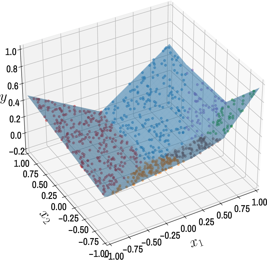
(a) True PWA function (39) and dataset

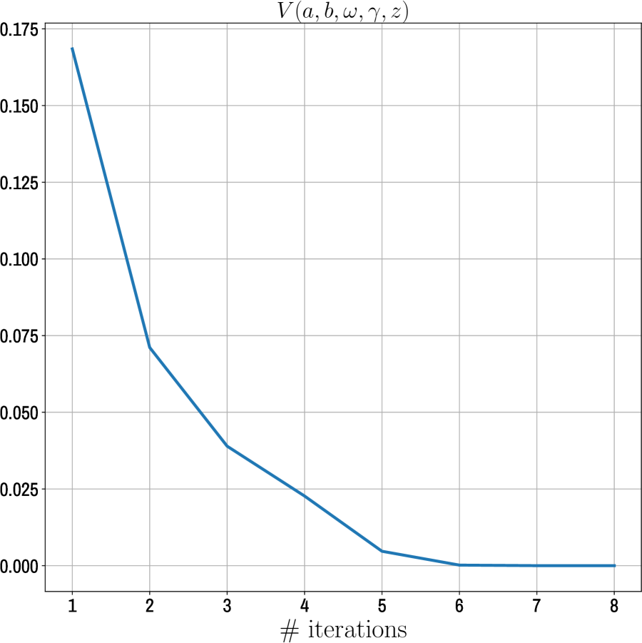
(b) Cost function during PARC iterations

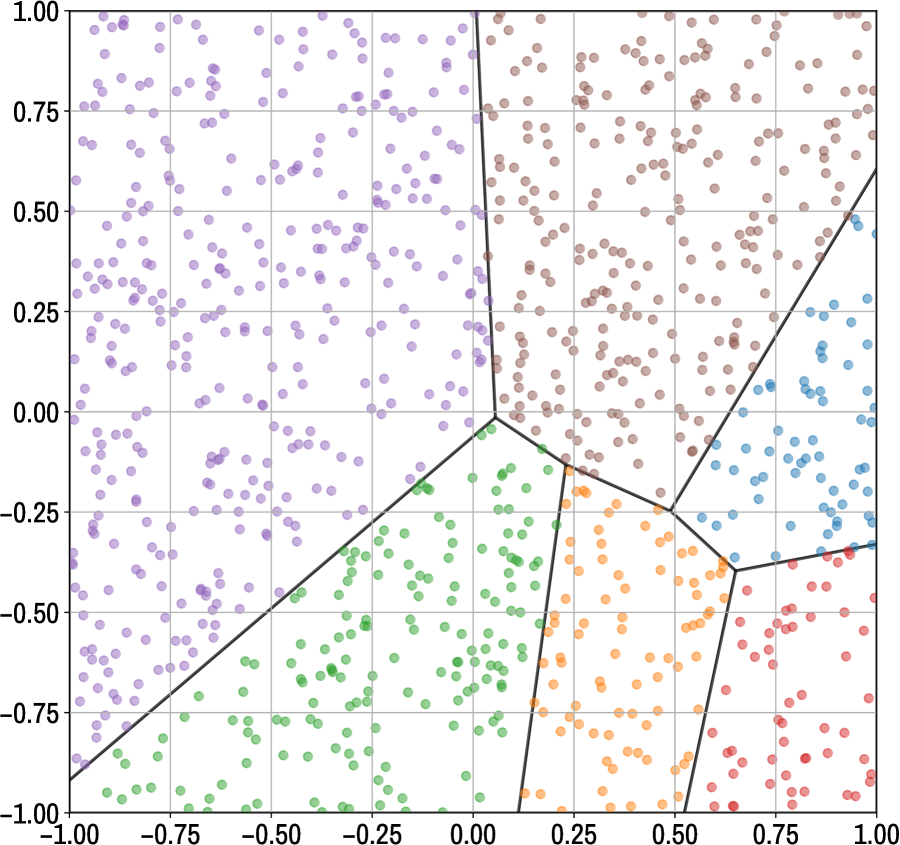
(c) True PWA partition induced by (39)

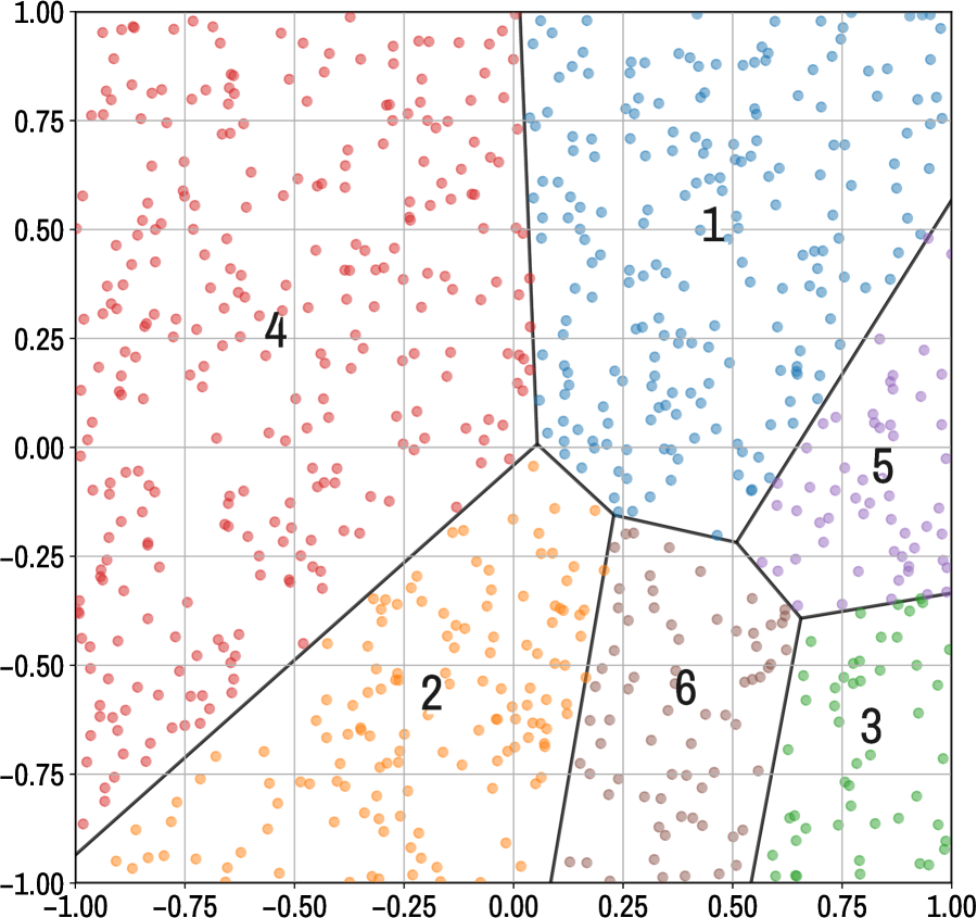
(d) PWA partition generated by PARC

Figure 1: PARC algorithm for regression on training data generated by the PWA function (39).

5.1.2 Nonlinear function

We solve another simple regression example on a dataset of $N=1000$ randomly-generated samples of the nonlinear function

$$y(x_{1},x_{2})=\sin\left(4x_{1}-5\left(x_{2}-\frac{1}{2}\right)^{2}\right)+2x_{2}$$ (40)

Again we use 80% of the samples as training data and the remaining 20% for testing. The function and the training dataset are shown in Figures 2, 3. We run PARC with $\sigma=1$, $\epsilon=10^{-4}$, PWL partitioning (23b) with $\beta=10^{-3}$, and different values of $K$. The level sets and training data are reported in Figure 2. The resulting piecewise linear regression functions are shown in Figure 3, which also shows the solution obtained by solving the MILP (4.1) for $y_{\rm ref}=3$.

The results obtained by running PARC for different values of $K$, $\sigma$ and the two alternative separation criteria (Voronoi partitioning and softmax regression with $\beta=10^{-3}$) are reported in Table 1 (R²-score on training data), Table 2 (R²-score on test data), Table 4 (CPU time [s] to execute PARC), Table 3 (number of PARC iterations). The best results are usually obtained for $\sigma=1$ using softmax regression (S) for PWL partitioning as in (23a).

The CPU time spent to solve the MILP (4.1) using the CBC solver through the Python MIP package  for $K$ = 3, 5, 8, 12, and 30 is, respectively, 8, 29, 85, 251, and 1420 ms. Note that the case $K=1$ corresponds to ridge regression on the entire dataset, while $\sigma=10000$ approximates the case $\sigma\rightarrow+\infty$, corresponding to pure PWL separation + ridge regression on each cluster.

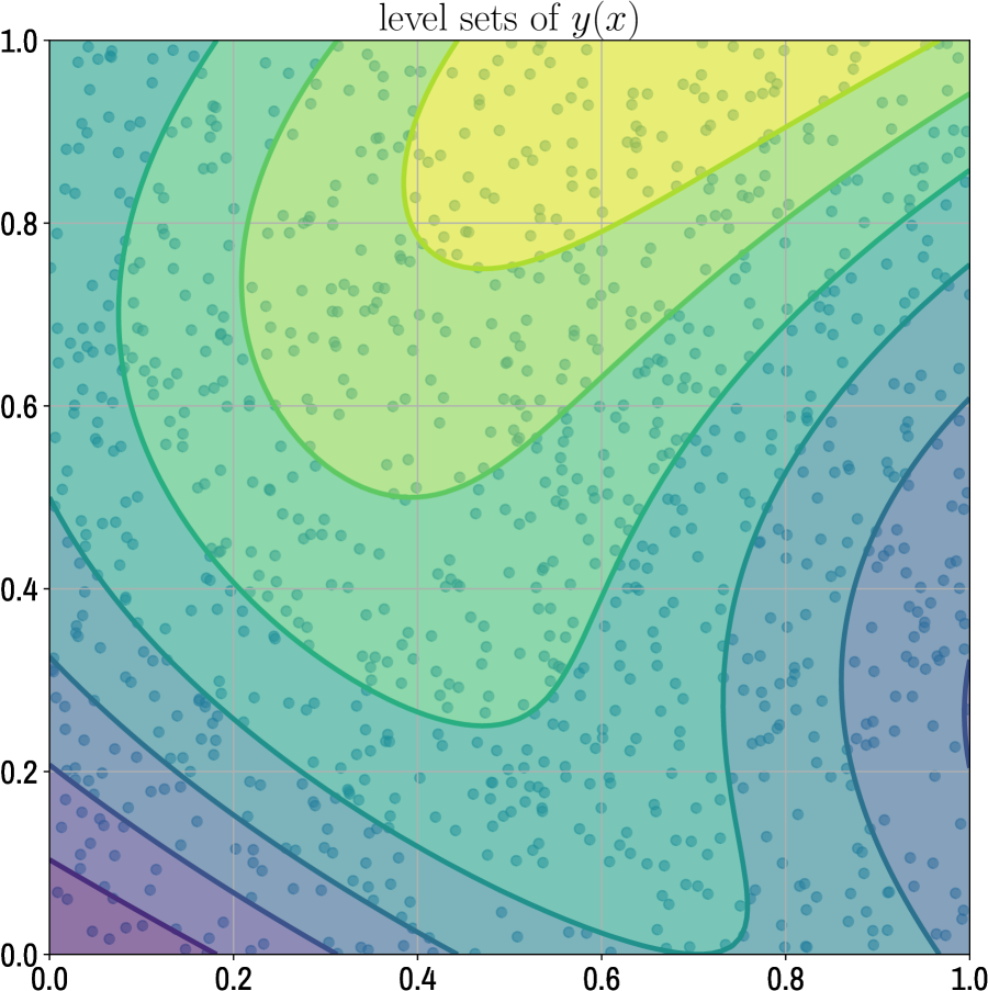
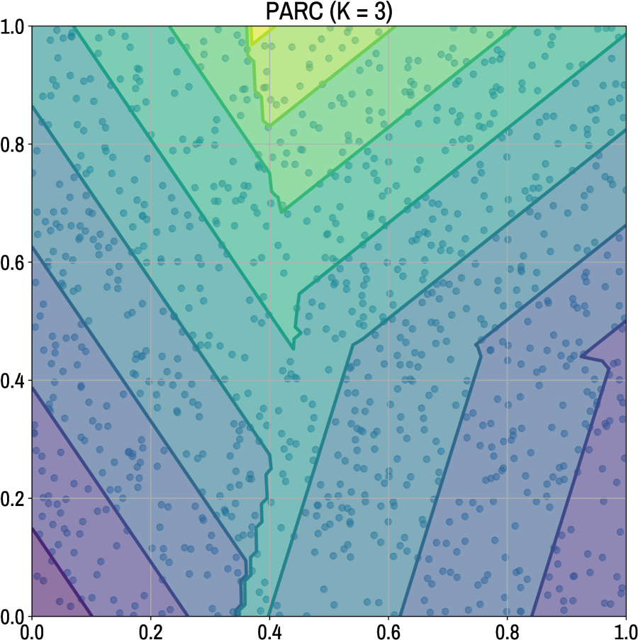
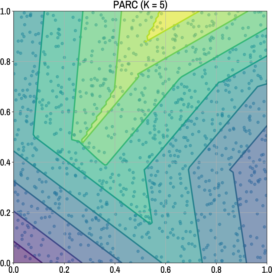
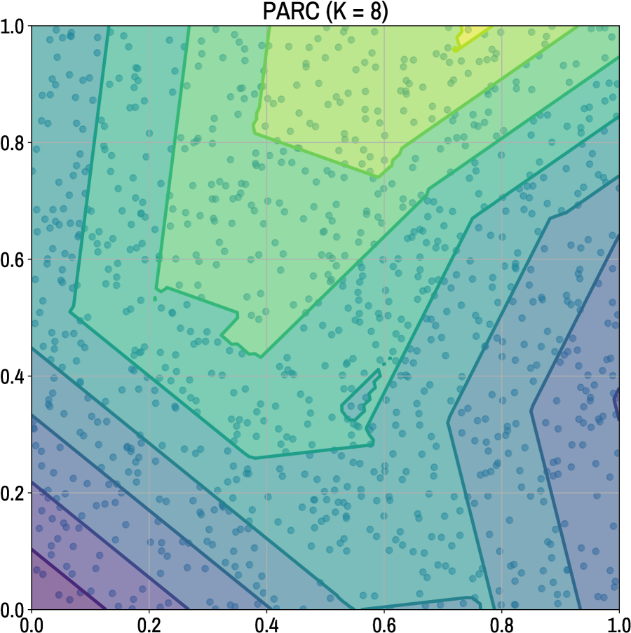
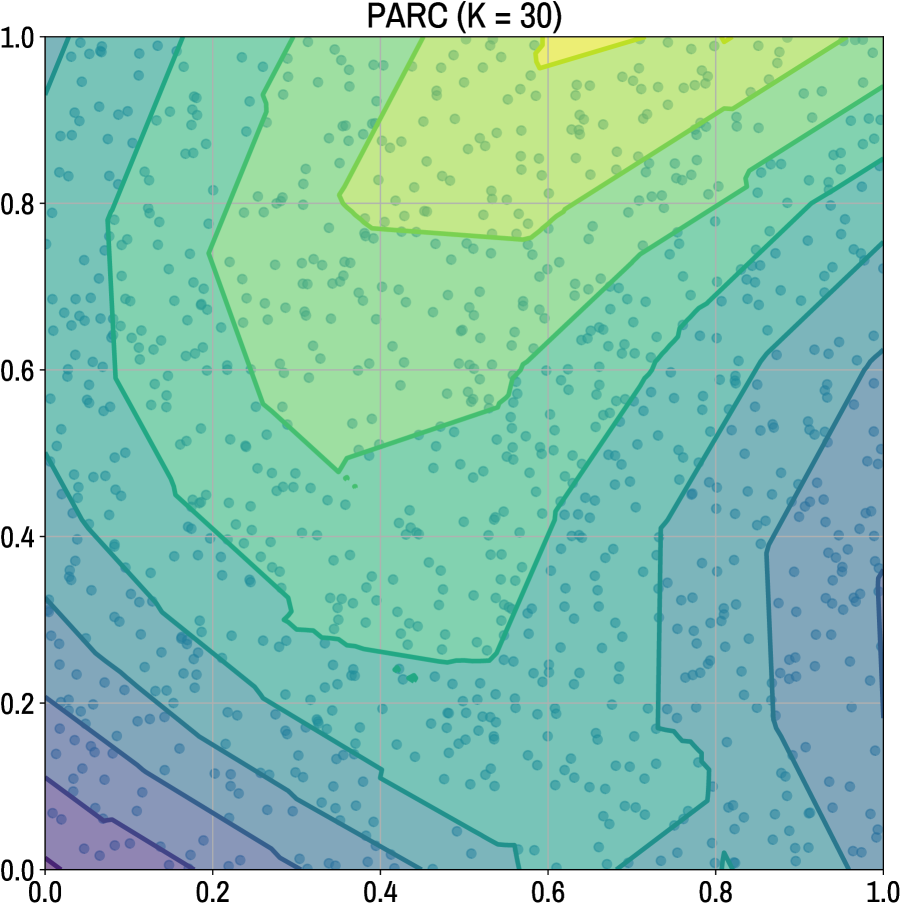
Figure 2: Training data and results of PARC for regression: nonlinear function (40).

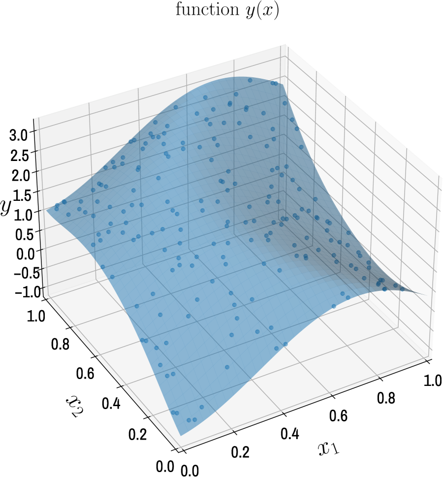
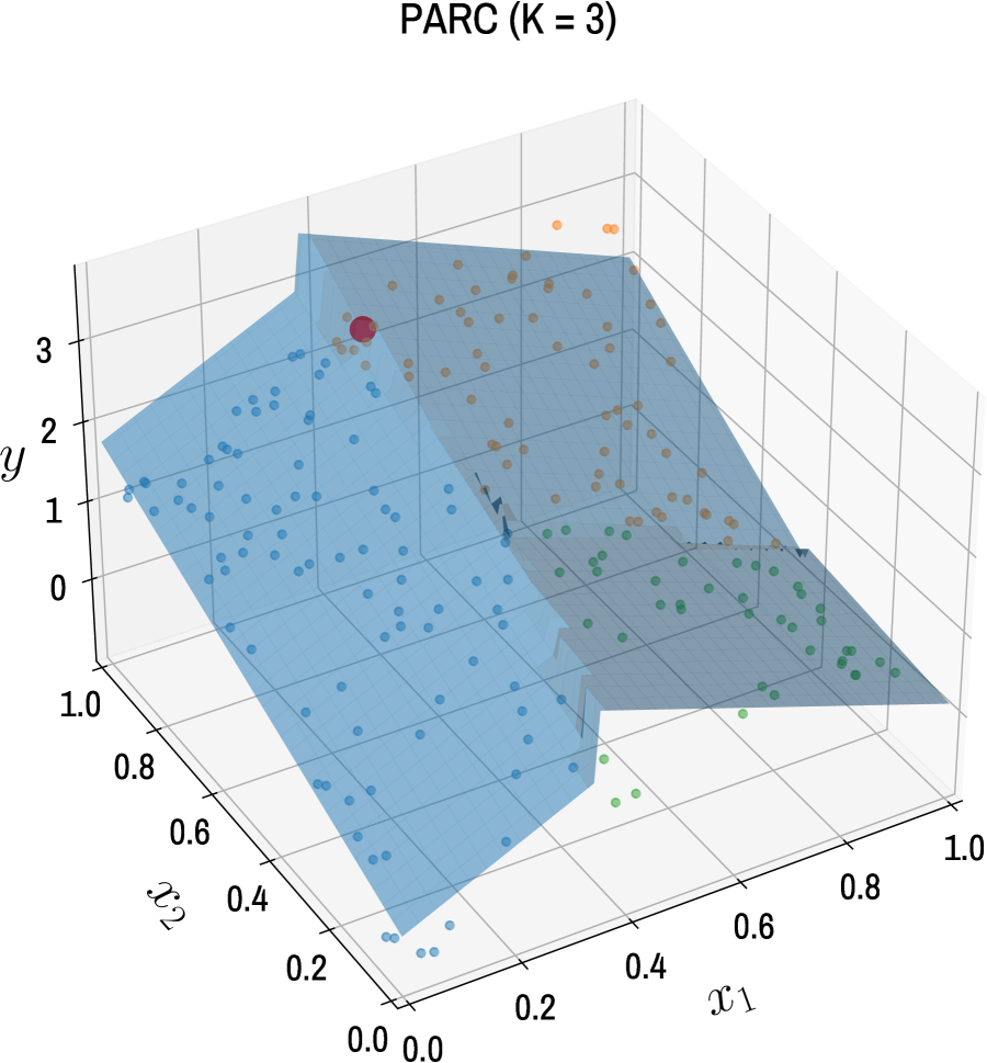
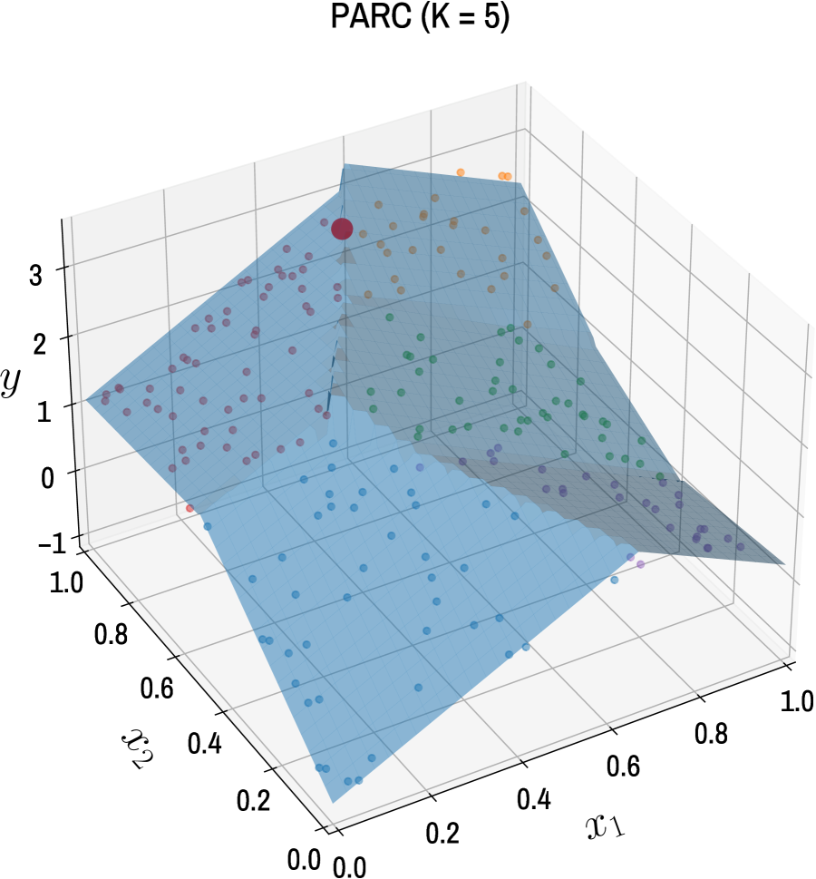
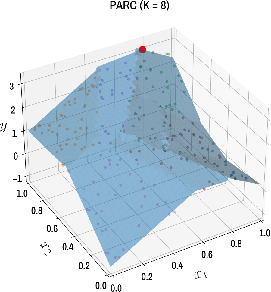
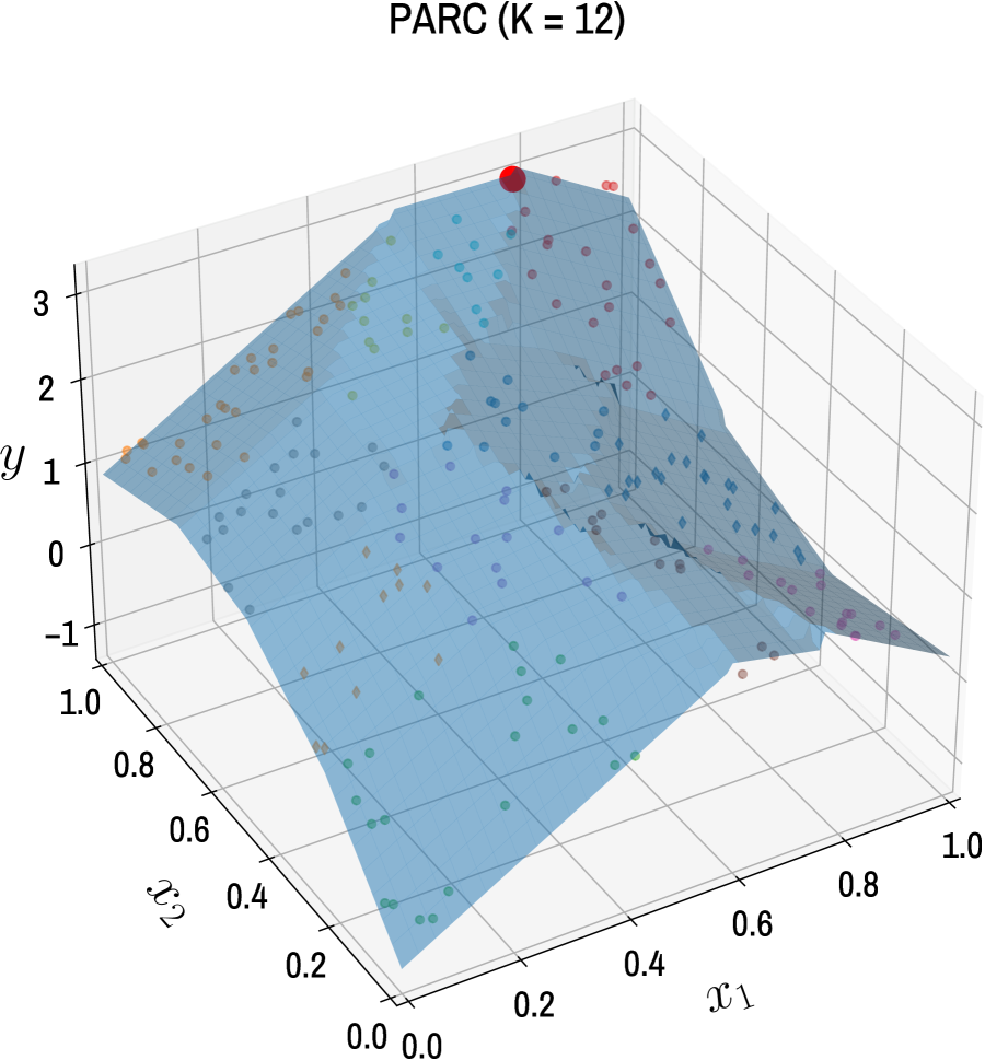
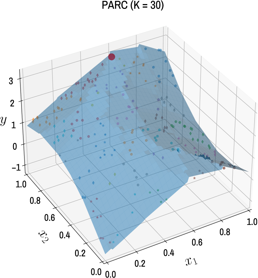
Figure 3: Training data and results of PARC for regression: nonlinear function (40). The result of the MILP optimization (4.1) is represented by the red dot.

$\sigma$	$K=1$	$K=3$	$K=5$	$K=8$	$K=12$	$K=30$
(S) 0	0.565 (1.4%)	0.899 (2.0%)	0.979 (0.2%)	0.991 (0.2%)	0.995 (0.2%)	0.998 (0.1%)
(V) 0	0.565 (1.4%)	0.886 (3.1%)	0.974 (0.3%)	0.986 (0.2%)	0.993 (0.2%)	0.998 (0.0%)
(S) 0.01	0.565 (1.4%)	0.899 (2.2%)	0.979 (0.2%)	0.991 (0.2%)	0.995 (0.1%)	0.999 (0.1%)
(V) 0.01	0.565 (1.4%)	0.887 (3.1%)	0.973 (0.3%)	0.986 (0.2%)	0.993 (0.1%)	0.998 (0.0%)
(S) 1	0.565 (1.4%)	0.895 (2.3%)	0.982 (0.2%)	0.994 (0.2%)	0.998 (0.0%)	0.999 (0.0%)
(V) 1	0.565 (1.4%)	0.881 (3.0%)	0.974 (0.3%)	0.986 (0.2%)	0.994 (0.1%)	0.999 (0.0%)
(S) 100	0.565 (1.4%)	0.908 (0.9%)	0.977 (0.5%)	0.986 (0.2%)	0.994 (0.1%)	0.999 (0.0%)
(V) 100	0.565 (1.4%)	0.887 (3.6%)	0.972 (0.4%)	0.989 (0.3%)	0.995 (0.0%)	0.999 (0.0%)
(S) 10000	0.565 (1.4%)	0.834 (2.1%)	0.969 (0.3%)	0.985 (0.2%)	0.994 (0.1%)	0.999 (0.0%)
(V) 10000	0.565 (1.4%)	0.865 (3.6%)	0.971 (0.3%)	0.985 (0.2%)	0.994 (0.1%)	0.999 (0.0%)

Table 1: PARC regression on targets from nonlinear function (40): R² score on training data, mean (std). PWL separation: (S) = softmax regression, (V) for Voronoi partitioning.

$\sigma$	$K=1$	$K=3$	$K=5$	$K=8$	$K=12$	$K=30$
(S) 0	0.548 (6.5%)	0.889 (2.6%)	0.976 (0.5%)	0.989 (0.3%)	0.994 (0.2%)	0.997 (0.1%)
(V) 0	0.548 (6.5%)	0.872 (3.6%)	0.970 (0.7%)	0.985 (0.4%)	0.993 (0.2%)	0.998 (0.1%)
(S) 0.01	0.548 (6.5%)	0.894 (2.5%)	0.976 (0.5%)	0.989 (0.4%)	0.994 (0.1%)	0.998 (0.1%)
(V) 0.01	0.548 (6.5%)	0.877 (3.3%)	0.969 (0.6%)	0.985 (0.3%)	0.992 (0.3%)	0.997 (0.1%)
(S) 1	0.548 (6.5%)	0.883 (2.8%)	0.981 (0.3%)	0.993 (0.2%)	0.997 (0.1%)	0.999 (0.0%)
(V) 1	0.548 (6.5%)	0.868 (3.5%)	0.970 (0.7%)	0.985 (0.3%)	0.993 (0.2%)	0.998 (0.1%)
(S) 100	0.548 (6.5%)	0.898 (1.6%)	0.970 (1.0%)	0.982 (0.2%)	0.992 (0.2%)	0.998 (0.0%)
(V) 100	0.548 (6.5%)	0.874 (4.1%)	0.967 (0.8%)	0.987 (0.4%)	0.993 (0.2%)	0.998 (0.1%)
(S) 10000	0.548 (6.5%)	0.816 (3.2%)	0.963 (0.8%)	0.980 (0.3%)	0.992 (0.1%)	0.998 (0.0%)
(V) 10000	0.548 (6.5%)	0.846 (4.4%)	0.965 (0.8%)	0.982 (0.3%)	0.993 (0.2%)	0.998 (0.0%)

Table 2: PARC regression on targets from nonlinear function (40): R² score on test data, mean (std). PWL separation: (S) = softmax regression, (V) for Voronoi partitioning.

$\sigma$	$K=1$	$K=3$	$K=5$	$K=8$	$K=12$	$K=30$
(S) 0	1.0 (0.0%)	18.9 (44.6%)	13.1 (27.3%)	16.9 (28.4%)	18.9 (22.8%)	13.0 (17.9%)
(V) 0	1.0 (0.0%)	20.2 (39.7%)	12.8 (26.3%)	17.1 (30.4%)	20.1 (27.4%)	13.9 (20.5%)
(S) 0.01	1.0 (0.0%)	17.7 (42.4%)	13.3 (37.0%)	17.4 (28.3%)	20.5 (39.6%)	12.3 (19.6%)
(V) 0.01	1.0 (0.0%)	17.8 (43.0%)	13.8 (32.7%)	14.3 (26.3%)	19.7 (31.5%)	14.5 (33.8%)
(S) 1	1.0 (0.0%)	19.2 (46.0%)	11.2 (27.2%)	15.5 (27.3%)	14.2 (17.8%)	7.9 (14.9%)
(V) 1	1.0 (0.0%)	19.4 (41.4%)	13.0 (39.1%)	15.1 (23.1%)	18.9 (36.4%)	12.5 (33.2%)
(S) 100	1.0 (0.0%)	19.4 (24.1%)	8.2 (36.3%)	5.8 (32.5%)	4.0 (37.8%)	5.2 (24.0%)
(V) 100	1.0 (0.0%)	17.4 (49.1%)	11.4 (41.7%)	17.2 (42.6%)	12.8 (23.5%)	8.9 (22.7%)
(S) 10000	1.0 (0.0%)	3.0 (31.2%)	3.1 (26.8%)	3.4 (30.0%)	4.6 (27.0%)	5.5 (29.9%)
(V) 10000	1.0 (0.0%)	11.7 (53.7%)	5.9 (45.8%)	4.5 (29.7%)	4.2 (37.1%)	3.5 (64.5%)

Table 3: PARC regression on targets from nonlinear function (40): number of PARC iterations, mean (std). PWL separation: (S) = softmax regression, (V) for Voronoi partitioning.

$\sigma$	$K=1$	$K=3$	$K=5$	$K=8$	$K=12$	$K=30$
(S) 0	0.12 (9.8%)	1.33 (43.6%)	1.46 (24.6%)	2.90 (28.0%)	5.18 (21.1%)	7.14 (17.3%)
(V) 0	0.04 (11.4%)	0.78 (36.1%)	0.77 (24.9%)	1.58 (30.7%)	2.64 (26.3%)	4.44 (19.5%)
(S) 0.01	0.12 (7.7%)	1.25 (40.3%)	1.48 (36.4%)	2.95 (30.1%)	5.47 (40.9%)	7.22 (18.7%)
(V) 0.01	0.04 (13.2%)	0.65 (41.2%)	0.82 (31.4%)	1.31 (25.1%)	2.58 (30.8%)	4.61 (32.8%)
(S) 1	0.12 (10.4%)	1.36 (43.8%)	1.42 (24.7%)	3.36 (26.0%)	4.14 (15.9%)	4.26 (14.9%)
(V) 1	0.04 (13.5%)	0.71 (38.6%)	0.78 (35.7%)	1.36 (22.7%)	2.48 (36.0%)	3.98 (31.1%)
(S) 100	0.12 (8.9%)	1.45 (24.2%)	1.11 (34.5%)	1.10 (30.4%)	1.04 (35.6%)	2.68 (22.1%)
(V) 100	0.04 (10.6%)	0.64 (44.9%)	0.69 (38.0%)	1.56 (43.5%)	1.70 (21.9%)	2.90 (21.0%)
(S) 10000	0.12 (9.2%)	0.24 (27.1%)	0.41 (22.6%)	0.66 (26.9%)	1.14 (24.2%)	2.80 (27.2%)
(V) 10000	0.04 (11.5%)	0.45 (49.7%)	0.38 (39.7%)	0.45 (24.8%)	0.62 (31.4%)	1.21 (61.8%)

Table 4: PARC regression on targets from nonlinear function (40): training time [s], mean (std). PWL separation: (S) = softmax regression, (V) for Voronoi partitioning.

5.2 Real-world datasets

We test the PARC algorithm on real-world datasets for regression and classification from the PMLB repository (Olson et al., 2017). The features containing four or less distinct values are treated as categorical and one-hot encoded, all the remaining features as numerical. In all tests, $N_{\rm tot}$ denotes the total number of samples in the dataset, whose 80% is used for training and the rest 20% for testing. PARC is run with $\sigma=1$, softmax regression for PWL partitioning (23a), $\epsilon=10^{-4}$, $\alpha=0.1$, $\beta=10^{-3}$. The minimum size of a cluster not to be discarded is 1% of the number $N$ of training samples. Prediction quality is measured in terms of $R^{2}$ score (in case of regression problems), or accuracy score $a$ (for classification), respectively defined as

$$R^{2}=1-\frac{\sum_{k=1}^{N}(y_{k}-\hat{y}(x_{k}))^{2}}{\sum_{k=1}^{N}(y_{k}-\frac{1}{N}\sum_{k=1}^{N}y_{k})^{2}},\quad a=\frac{1}{N}\sum_{k=1}^{N}[\hat{y}(x_{k})=y_{k}]$$

The neural networks and decision trees used for comparison are trained using scikit-learn (Pedregosa et al., 2011) functions. The stochastic optimizer Adam (Kingma and Ba, 2015) is used for training the coefficient and bias terms of the neural network.

5.2.1 Regression problems

We extracted all the datasets from the PMLB repository with numeric targets containing between $N_{\rm tot}=500$ and $5000$ samples and between $n_{x}=2$ and $20$ features (before one-hot encoding categorical features). Five-fold cross-validation is run on the training dataset for all values of $K$ between $2$ and $15$ to determine the value $K^{*}$ that is optimal in terms of average $R^{2}$ score. For comparison, we run PARC with fixed values of $K$ and compare against other methods providing piecewise linear partitions, particularly a neural network with ReLU activation function with a single layer of $K^{*}$ neurons and a decision tree with ten non-leaf nodes. Note that the neural network requires $K^{*}$ binary variables to encode the ReLU activation functions in a MIP, the same number as the PWL regressor determined by PARC, as described in Section 4.1. In contrast, the decision tree requires ten binary variables.

The $R^{2}$ scores obtained on the datasets are shown in Table 5 (training data) and in Table 6 (test data). The CPU time spent on solving the training problems is reported in Table 7.

The results show that PARC often provides better fit on training data, especially for large values of $K$. On test data, PARC and neural networks with $K^{*}$ ReLU neurons provide the best results. Some poor results of PARC on test data for large values of $K$ are usually associated with overfitting the training dataset, see for example 522_pm10, 547_no2, 627_fri_C1_1000_5.

5.2.2 Classification problems

We extracted all datasets from the PMLB repository with categorical targets with at most $m_{1}=10$ classes, containing between $N_{\rm tot}=1000$ and 5000 samples, and between $n_{x}=2$ and 20 features (before one-hot encoding categorical features). We compare PARC with $K=2$, $3$, $5$ to softmax regression (corresponding to setting $K=1$ in PARC), a neural network (NN) with ReLU activation function and a single layer of $K=5$ neurons, and a decision tree (DT) with $5$ non-leaf nodes. Encoding the PARC classifier as an MIP requires $K+m_{1}$ binary variables as described in Section 4.1, the NN requires $5+m_{1}$ binary variables for MIP encoding, the DT requires $5+m_{1}$ binary variables ($m_{1}$ variables are required to encode the $\arg\max$ selecting the class with highest score). In this test campaign, computing $K^{*}$ by cross-validation has not shown to bring significant benefits and is not reported.

The accuracy scores obtained on the datasets are shown in Table 8 (training data) and in Table 9 (test data). The CPU time spent on solving the training problems is reported in Table 10. On training data, PARC with $K=5$ provides the best accuracy in about 75% of the datasets, with neural networks based on $5$ ReLU neurons better performing in the remaining cases. On test data, most methods perform similarly, with neural networks providing slightly superior accuracy.

6 Conclusions

The regression and classification algorithm proposed in this paper generalizes linear regression and classification approaches, in particular, ridge regression and softmax regression, to a piecewise linear form. Such a form is amenable for mixed-integer encoding, particularly beneficial when the obtained predictor becomes part of an optimization model. Results on synthetic and real-world datasets show that the accuracy of the method is comparable to that of alternative approaches that admit a piecewise linear form of similar complexity. A possible drawback of PARC is its computation time, mainly due to solving a sequence of softmax regression problems. This makes PARC applicable to datasets whose size, in terms of number of samples and features, is such that standard softmax regression is a feasible approach.

Other regression and classification methods, such as deep neural networks, more complex decision trees, and even random forests may achieve better scores on test data and reduced training time. However, they would return predictors that are more complicated to optimize over the predictor than the proposed piecewise linear models.

The proposed algorithm can be extended in several ways. For example, $\ell_{1}$-penalties can be introduced in (28) to promote sparsity of $a,b$. The proof of Theorem 1 can be easily extended to cover such a modification. Moreover, basis functions $\phi_{i}(x)$ can be used instead of $x$ directly, such as canonical piecewise linear functions (Lin and Unbehauen, 1992; Chua and Deng, 1988; Julián et al., 2000) to maintain the PWL nature of the predictor, with possibly different basis functions chosen for partitioning the feature space and for fitting targets.

The proposed algorithm is also extendable to other regression, classification, and separation methods than linear ones, as long as we can associate a suitable cost function $V^{y}$/$V^{x}$. As an example, neural networks with ReLU activation functions might be used instead of ridge regression for extended flexibility, for which we can define $V_{y}(a^{j},b^{j},x_{k},y_{k})$ as the loss computed on the training data of cluster #$j$.

Ongoing research is devoted to alternative methods to obtain the initial assignment of datapoints to clusters, as this is a crucial step that affects the quality of the minimum PARC converges to, and to applying the proposed method to data-driven model predictive control of hybrid dynamical systems.

dataset	PARC	PARC	PARC	PARC	ridge	NN	DT
$N_{\rm tot}$, $n_{x}$, $K^{*}$	$K^{*}$	$K=3$	$K=5$	$K=12$	$K=1$	$K^{*}$	$10$
1028_SWD	0.466	0.484	0.515	0.529	0.441	0.423	0.388
1000, 21, 2	(1.2%)	(1.2%)	(1.2%)	(1.2%)	(1.1%)	(6.9%)	(1.8%)
1029_LEV	0.589	0.600	0.612	0.623	0.577	0.561	0.466
1000, 16, 2	(1.4%)	(1.5%)	(1.5%)	(1.3%)	(1.4%)	(2.3%)	(1.7%)
1030_ERA	0.427	0.427	0.427	0.427	0.427	0.321	0.347
1000, 51, 2	(1.4%)	(1.4%)	(1.4%)	(1.4%)	(1.4%)	(10.3%)	(1.4%)
522_pm10	0.382	0.419	0.515	0.768	0.246	0.280	0.423
500, 29, 2	(2.3%)	(3.1%)	(3.3%)	(3.2%)	(1.8%)	(7.6%)	(1.6%)
529_pollen	0.796	0.794	0.794	0.796	0.793	0.793	0.486
3848, 4, 15	(0.3%)	(0.2%)	(0.2%)	(0.2%)	(0.2%)	(0.3%)	(0.7%)
547_no2	0.630	0.666	0.706	0.855	0.559	0.563	0.612
500, 29, 2	(1.8%)	(1.8%)	(1.7%)	(1.4%)	(1.7%)	(3.0%)	(1.6%)
593_fri_c1_1000_10	0.766	0.636	0.755	0.828	0.306	0.689	0.751
1000, 10, 5	(10.3%)	(7.2%)	(10.6%)	(4.1%)	(1.0%)	(28.0%)	(0.9%)
595_fri_c0_1000_10	0.835	0.805	0.836	0.893	0.722	0.805	0.677
1000, 10, 4	(2.7%)	(2.1%)	(2.4%)	(1.1%)	(0.7%)	(4.8%)	(1.1%)
597_fri_c2_500_5	0.934	0.622	0.907	0.945	0.282	0.930	0.821
500, 5, 11	(1.9%)	(8.6%)	(2.4%)	(2.3%)	(1.5%)	(1.2%)	(0.8%)
599_fri_c2_1000_5	0.933	0.698	0.849	0.937	0.312	0.942	0.791
1000, 5, 10	(1.3%)	(10.7%)	(7.9%)	(0.9%)	(1.0%)	(0.5%)	(0.8%)
604_fri_c4_500_10	0.837	0.698	0.829	0.891	0.297	0.806	0.757
500, 10, 7	(7.2%)	(8.2%)	(7.1%)	(3.3%)	(2.1%)	(20.6%)	(1.1%)
606_fri_c2_1000_10	0.766	0.617	0.783	0.855	0.329	0.488	0.771
1000, 10, 4	(5.4%)	(10.9%)	(5.0%)	(4.4%)	(1.2%)	(22.1%)	(0.9%)
608_fri_c3_1000_10	0.842	0.494	0.854	0.872	0.305	0.901	0.748
1000, 10, 7	(4.6%)	(7.5%)	(2.8%)	(3.7%)	(1.2%)	(8.6%)	(1.2%)
609_fri_c0_1000_5	0.936	0.821	0.877	0.934	0.730	0.909	0.676
1000, 5, 15	(0.7%)	(2.8%)	(2.3%)	(0.6%)	(0.8%)	(1.6%)	(0.8%)
612_fri_c1_1000_5	0.909	0.563	0.750	0.898	0.264	0.943	0.746
1000, 5, 14	(2.6%)	(24.3%)	(11.8%)	(4.2%)	(0.9%)	(0.4%)	(0.7%)
617_fri_c3_500_5	0.906	0.820	0.879	0.927	0.270	0.892	0.780
500, 5, 10	(2.8%)	(6.4%)	(2.2%)	(2.1%)	(1.6%)	(1.0%)	(1.2%)
623_fri_c4_1000_10	0.854	0.675	0.852	0.887	0.300	0.870	0.746
1000, 10, 6	(5.9%)	(8.5%)	(5.0%)	(2.3%)	(1.1%)	(16.2%)	(1.0%)
627_fri_c2_500_10	0.711	0.624	0.725	0.841	0.301	0.455	0.798
500, 10, 5	(7.6%)	(17.5%)	(8.3%)	(4.7%)	(1.2%)	(21.1%)	(1.1%)
628_fri_c3_1000_5	0.934	0.550	0.907	0.937	0.268	0.903	0.738
1000, 5, 7	(0.9%)	(9.7%)	(1.8%)	(0.8%)	(0.9%)	(7.0%)	(0.9%)
631_fri_c1_500_5	0.904	0.901	0.777	0.916	0.294	0.842	0.757
500, 5, 9	(3.4%)	(0.8%)	(10.4%)	(2.7%)	(2.0%)	(18.1%)	(0.8%)
641_fri_c1_500_10	0.746	0.798	0.768	0.823	0.288	0.371	0.789
500, 10, 3	(18.4%)	(13.5%)	(6.9%)	(3.6%)	(1.6%)	(21.4%)	(1.0%)
646_fri_c3_500_10	0.877	0.643	0.886	0.894	0.357	0.706	0.774
500, 10, 5	(5.4%)	(12.3%)	(2.9%)	(3.0%)	(1.9%)	(23.3%)	(1.8%)
649_fri_c0_500_5	0.928	0.824	0.893	0.936	0.738	0.886	0.717
500, 5, 10	(0.9%)	(3.3%)	(1.7%)	(1.0%)	(1.1%)	(2.0%)	(1.2%)
654_fri_c0_500_10	0.822	0.797	0.825	0.890	0.700	0.797	0.697
500, 10, 5	(2.5%)	(2.3%)	(2.1%)	(2.3%)	(1.3%)	(4.8%)	(1.4%)
666_rmftsa_ladata	0.660	0.671	0.723	0.811	0.581	0.525	0.732
508, 10, 2	(4.1%)	(3.0%)	(3.2%)	(2.1%)	(2.2%)	(10.3%)	(2.2%)
titanic	0.278	0.295	0.296	0.279	0.253	0.292	0.300
2201, 5, 12	(1.1%)	(1.2%)	(1.1%)	(1.1%)	(1.1%)	(1.1%)	(0.8%)

Table 5: Real-world datasets for regression: average $R^{2}$ score (standard deviation) over 20 runs on training data (best result is highlighted in boldface).

dataset	PARC	PARC	PARC	PARC	ridge	NN	DT
$N_{\rm tot}$, $n_{x}$, $K^{*}$	$K^{*}$	$K=3$	$K=5$	$K=12$	$K=1$	$K^{*}$	$10$
1028_SWD	0.413	0.403	0.383	0.372	0.425	0.423	0.334
1000, 21, 2	(4.6%)	(5.0%)	(4.8%)	(5.1%)	(4.6%)	(6.9%)	(4.2%)
1029_LEV	0.536	0.533	0.519	0.510	0.542	0.561	0.412
1000, 16, 2	(6.2%)	(6.7%)	(7.1%)	(7.6%)	(6.5%)	(2.3%)	(8.3%)
1030_ERA	0.339	0.339	0.339	0.339	0.339	0.321	0.269
1000, 51, 2	(6.7%)	(6.7%)	(6.7%)	(6.7%)	(6.8%)	(10.3%)	(6.5%)
522_pm10	0.095	0.043	-0.048	-0.896	0.095	0.280	0.177
500, 29, 2	(12.3%)	(12.2%)	(14.4%)	(61.6%)	(8.1%)	(7.6%)	(11.5%)
529_pollen	0.793	0.796	0.796	0.793	0.796	0.793	0.438
3848, 4, 15	(1.0%)	(1.0%)	(1.0%)	(0.9%)	(1.0%)	(0.3%)	(1.7%)
547_no2	0.478	0.468	0.403	-0.189	0.488	0.563	0.420
500, 29, 2	(9.0%)	(11.0%)	(12.2%)	(32.1%)	(8.3%)	(3.0%)	(7.1%)
593_fri_c1_1000_10	0.696	0.582	0.694	0.693	0.292	0.689	0.671
1000, 10, 5	(12.4%)	(9.1%)	(12.4%)	(8.6%)	(3.8%)	(28.0%)	(3.4%)
595_fri_c0_1000_10	0.804	0.760	0.788	0.813	0.693	0.805	0.585
1000, 10, 4	(3.8%)	(4.9%)	(3.2%)	(3.8%)	(3.1%)	(4.8%)	(2.9%)
597_fri_c2_500_5	0.889	0.570	0.888	0.891	0.274	0.930	0.701
500, 5, 11	(7.0%)	(11.0%)	(4.8%)	(4.6%)	(6.7%)	(1.2%)	(5.3%)
599_fri_c2_1000_5	0.920	0.674	0.828	0.924	0.277	0.942	0.724
1000, 5, 10	(1.9%)	(12.4%)	(9.8%)	(1.5%)	(4.2%)	(0.5%)	(2.9%)
604_fri_c4_500_10	0.579	0.596	0.624	0.433	0.235	0.806	0.610
500, 10, 7	(23.1%)	(13.0%)	(13.6%)	(42.2%)	(10.0%)	(20.6%)	(6.1%)
606_fri_c2_1000_10	0.710	0.575	0.725	0.700	0.302	0.488	0.712
1000, 10, 4	(8.0%)	(11.0%)	(7.8%)	(9.6%)	(5.4%)	(22.1%)	(3.0%)
608_fri_c3_1000_10	0.766	0.420	0.804	0.729	0.269	0.901	0.658
1000, 10, 7	(8.5%)	(9.9%)	(3.9%)	(9.5%)	(5.4%)	(8.6%)	(4.9%)
609_fri_c0_1000_5	0.918	0.811	0.861	0.917	0.725	0.909	0.580
1000, 5, 15	(1.5%)	(3.5%)	(3.6%)	(1.5%)	(3.1%)	(1.6%)	(3.4%)
612_fri_c1_1000_5	0.877	0.524	0.725	0.865	0.256	0.943	0.690
1000, 5, 14	(4.5%)	(26.0%)	(12.8%)	(7.1%)	(3.4%)	(0.4%)	(2.5%)
617_fri_c3_500_5	0.806	0.781	0.814	0.831	0.206	0.892	0.622
500, 5, 10	(5.6%)	(7.8%)	(7.5%)	(7.7%)	(7.2%)	(1.0%)	(6.0%)
623_fri_c4_1000_10	0.775	0.642	0.814	0.766	0.291	0.870	0.659
1000, 10, 6	(11.6%)	(10.2%)	(8.3%)	(10.7%)	(4.9%)	(16.2%)	(3.9%)
627_fri_c2_500_10	0.547	0.521	0.587	0.375	0.252	0.455	0.654
500, 10, 5	(16.5%)	(23.0%)	(11.3%)	(24.0%)	(6.1%)	(21.1%)	(6.0%)
628_fri_c3_1000_5	0.928	0.554	0.902	0.921	0.278	0.903	0.651
1000, 5, 7	(2.5%)	(9.0%)	(2.2%)	(2.2%)	(3.6%)	(7.0%)	(2.9%)
631_fri_c1_500_5	0.857	0.883	0.735	0.828	0.266	0.842	0.674
500, 5, 9	(5.6%)	(2.5%)	(15.3%)	(7.8%)	(8.9%)	(18.1%)	(6.5%)
641_fri_c1_500_10	0.658	0.730	0.659	0.350	0.253	0.371	0.690
500, 10, 3	(27.2%)	(21.7%)	(14.7%)	(19.8%)	(7.8%)	(21.4%)	(4.1%)
646_fri_c3_500_10	0.767	0.547	0.791	0.552	0.295	0.706	0.616
500, 10, 5	(10.0%)	(16.4%)	(8.3%)	(15.0%)	(9.0%)	(23.3%)	(6.9%)
649_fri_c0_500_5	0.881	0.782	0.859	0.874	0.706	0.886	0.585
500, 5, 10	(3.0%)	(7.0%)	(4.0%)	(3.8%)	(5.2%)	(2.0%)	(6.0%)
654_fri_c0_500_10	0.708	0.729	0.722	0.604	0.656	0.797	0.569
500, 10, 5	(5.2%)	(5.5%)	(4.3%)	(15.7%)	(5.7%)	(4.8%)	(6.4%)
666_rmftsa_ladata	0.605	0.600	0.586	0.424	0.569	0.525	0.436
508, 10, 2	(11.0%)	(7.2%)	(11.6%)	(21.5%)	(7.9%)	(10.3%)	(17.7%)
titanic	0.263	0.280	0.280	0.264	0.248	0.292	0.273
2201, 5, 12	(4.0%)	(4.3%)	(4.3%)	(3.8%)	(4.4%)	(1.1%)	(3.1%)

Table 6: Real-world datasets for regression: average $R^{2}$ score (standard deviation) over 20 runs on test data (best result is highlighted in boldface).

	PARC	PARC	PARC	PARC	ridge	NN	DT
dataset	$K^{*}$	$K=3$	$K=5$	$K=12$	$K=1$	$K^{*}$	$10$
1028_SWD	0.6666	1.1096	1.7139	3.2273	0.0006	0.5088	0.0005
1029_LEV	0.5621	1.0421	1.6887	3.3071	0.0005	0.5423	0.0007
1030_ERA	0.4840	1.1526	2.3644	3.9153	0.0007	0.3873	0.0021
522_pm10	0.6238	1.0649	1.5356	2.8125	0.0004	0.3289	0.0011
529_pollen	12.2727	4.3129	5.6963	10.3119	0.0003	0.3802	0.0038
547_no2	0.7249	0.9619	1.5235	2.7249	0.0006	0.3504	0.0011
593_fri_c1_1000_10	1.8327	1.1290	1.8705	3.5305	0.0003	0.8015	0.0022
595_fri_c0_1000_10	1.5308	1.3855	1.7471	3.2421	0.0004	0.4898	0.0022
597_fri_c2_500_5	1.3449	0.4908	0.7735	1.3944	0.0003	0.4973	0.0009
599_fri_c2_1000_5	2.5124	1.1925	1.5406	2.8690	0.0005	0.6089	0.0012
604_fri_c4_500_10	1.0416	0.7536	0.9042	1.4882	0.0005	0.7006	0.0010
606_fri_c2_1000_10	1.5651	1.3613	1.8140	3.3661	0.0004	0.5473	0.0021
608_fri_c3_1000_10	2.1771	1.3441	1.9553	3.7203	0.0004	0.9239	0.0020
609_fri_c0_1000_5	3.0561	1.0232	1.4174	2.5315	0.0003	0.3431	0.0012
612_fri_c1_1000_5	3.3496	1.1189	1.5416	2.9122	0.0003	0.5835	0.0012
617_fri_c3_500_5	1.5364	0.6323	0.9217	1.7485	0.0003	0.5978	0.0007
623_fri_c4_1000_10	2.1292	1.4544	1.9706	3.7491	0.0005	0.9320	0.0022
627_fri_c2_500_10	0.7763	0.7443	0.8311	1.2776	0.0007	0.4008	0.0010
628_fri_c3_1000_5	2.1933	1.2742	1.7093	3.3434	0.0007	0.7285	0.0012
631_fri_c1_500_5	1.3440	0.6531	0.8145	1.5589	0.0004	0.5135	0.0006
641_fri_c1_500_10	0.6197	0.6375	0.7895	1.4259	0.0005	0.3879	0.0011
646_fri_c3_500_10	0.8552	0.6777	0.8998	1.4902	0.0005	0.5253	0.0012
649_fri_c0_500_5	1.0869	0.5163	0.7222	1.2470	0.0005	0.2539	0.0000
654_fri_c0_500_10	0.7623	0.5628	0.7580	1.2344	0.0005	0.3452	0.0010
666_rmftsa_ladata	0.4828	0.6842	0.9532	1.6299	0.0003	0.4306	0.0009
titanic	1.3399	0.8540	0.9237	1.3155	0.0003	0.3517	0.0004

Table 7: Real-world datasets for regression: average CPU time (s) over 20 runs on regression data.

dataset	PARC	PARC	PARC	softmax	NN	DT
$N_{\rm tot}$, $n_{x}$, $m_{1}$	$K=2$	$K=3$	$K=5$	$K=1$	$5$	$5$
car	0.96	0.97	0.98	0.95	0.97	0.84
1728, 15, 4	(0.8%)	(1.0%)	(1.1%)	(0.4%)	(1.0%)	(0.6%)
churn	0.91	0.90	0.90	0.87	0.93	0.94
5000, 21, 2	(1.9%)	(1.3%)	(1.0%)	(0.2%)	(1.3%)	(0.2%)
cmc	0.58	0.57	0.60	0.53	0.59	0.58
1473, 17, 3	(1.0%)	(1.3%)	(1.4%)	(0.9%)	(1.7%)	(0.7%)
contraceptive	0.59	0.58	0.60	0.53	0.59	0.58
1473, 17, 3	(1.0%)	(0.8%)	(1.0%)	(0.7%)	(2.6%)	(0.7%)
credit_g	0.79	0.82	0.88	0.77	0.85	0.78
1000, 37, 2	(0.7%)	(1.2%)	(1.3%)	(0.9%)	(1.2%)	(0.9%)
flare	0.84	0.85	0.85	0.84	0.84	0.85
1066, 13, 2	(0.7%)	(0.7%)	(0.9%)	(0.5%)	(0.6%)	(0.7%)
GAMETES_E**0.1H	0.64	0.64	0.70	0.56	0.75	0.57
1600, 40, 2	(1.8%)	(1.3%)	(1.2%)	(1.0%)	(1.1%)	(1.8%)
GAMETES_E**0.4H	0.69	0.72	0.80	0.55	0.84	0.54
1600, 38, 2	(6.3%)	(4.8%)	(5.0%)	(1.0%)	(0.8%)	(1.7%)
GAMETES_E**0.2H	0.62	0.64	0.69	0.58	0.68	0.57
1600, 40, 2	(1.1%)	(1.1%)	(1.1%)	(0.9%)	(1.9%)	(0.7%)
GAMETES_H**_50	0.62	0.64	0.70	0.55	0.77	0.57
1600, 39, 2	(2.0%)	(2.0%)	(2.0%)	(0.8%)	(1.5%)	(2.4%)
GAMETES_H**_75	0.63	0.70	0.73	0.56	0.79	0.56
1600, 39, 2	(2.1%)	(3.5%)	(3.2%)	(0.9%)	(1.3%)	(2.8%)
german	0.80	0.83	0.88	0.77	0.85	0.78
1000, 37, 2	(0.8%)	(1.1%)	(1.2%)	(0.8%)	(1.3%)	(1.0%)
led7	0.75	0.75	0.75	0.75	0.73	0.69
3200, 7, 10	(0.6%)	(0.6%)	(0.5%)	(0.6%)	(1.5%)	(0.7%)
mfeat_morphological	0.77	0.77	0.77	0.76	0.74	0.72
2000, 7, 10	(0.5%)	(0.5%)	(0.6%)	(0.5%)	(2.1%)	(0.8%)
mofn_3_7_10	1.00	1.00	1.00	1.00	1.00	0.88
1324, 10, 2	(0.0%)	(0.0%)	(0.0%)	(0.0%)	(0.0%)	(0.5%)
parity5+5	0.55	0.59	0.69	0.52	0.61	0.54
1124, 10, 2	(2.6%)	(8.0%)	(13.8%)	(1.3%)	(14.4%)	(1.4%)
segmentation	0.97	0.98	0.98	0.97	0.97	0.94
2310, 21, 7	(0.5%)	(0.5%)	(0.3%)	(0.3%)	(0.5%)	(0.3%)
solar_flare_2	0.79	0.80	0.81	0.78	0.78	0.77
1066, 16, 6	(0.8%)	(0.9%)	(0.8%)	(0.8%)	(1.2%)	(0.9%)
wine_quality_red	0.62	0.64	0.66	0.61	0.62	0.62
1599, 11, 6	(1.0%)	(1.0%)	(1.2%)	(0.5%)	(1.1%)	(1.3%)
wine_quality_white	0.55	0.55	0.57	0.54	0.56	0.54
4898, 11, 7	(0.4%)	(0.6%)	(0.7%)	(0.3%)	(0.4%)	(0.6%)
yeast	0.61	0.62	0.64	0.60	0.60	0.61
1479, 9, 9	(0.8%)	(1.0%)	(1.1%)	(0.7%)	(1.0%)	(1.0%)

Table 8: Real-world datasets for classification: average accuracy score (standard deviation) over 20 runs on training data (best result is highlighted in boldface).

dataset	PARC	PARC	PARC	softmax	NN	DT
$N_{\rm tot}$, $n_{x}$, $m_{1}$	$K=2$	$K=3$	$K=5$	$K=1$	$5$	$5$
car	0.94	0.94	0.95	0.93	0.95	0.81
1728, 15, 4	(1.7%)	(1.1%)	(2.1%)	(1.2%)	(2.0%)	(1.7%)
churn	0.90	0.89	0.88	0.86	0.92	0.93
5000, 21, 2	(1.6%)	(1.9%)	(1.0%)	(0.8%)	(1.6%)	(0.7%)
cmc	0.55	0.53	0.52	0.51	0.56	0.56
1473, 17, 3	(2.9%)	(2.9%)	(2.5%)	(3.3%)	(2.6%)	(2.6%)
contraceptive	0.54	0.52	0.52	0.50	0.54	0.56
1473, 17, 3	(2.6%)	(2.1%)	(2.3%)	(2.4%)	(2.9%)	(2.9%)
credit_g	0.73	0.72	0.69	0.74	0.72	0.73
1000, 37, 2	(2.5%)	(3.3%)	(2.4%)	(2.9%)	(2.8%)	(2.6%)
flare	0.82	0.82	0.82	0.83	0.83	0.81
1066, 13, 2	(2.3%)	(2.4%)	(2.8%)	(2.6%)	(2.2%)	(2.6%)
GAMETES_E**0.1H	0.54	0.51	0.53	0.48	0.62	0.50
1600, 40, 2	(3.6%)	(2.3%)	(3.5%)	(2.7%)	(2.6%)	(2.9%)
GAMETES_E**0.4H	0.62	0.63	0.68	0.47	0.75	0.49
1600, 38, 2	(8.8%)	(7.2%)	(6.5%)	(2.6%)	(2.4%)	(2.7%)
GAMETES_E**0.2H	0.51	0.51	0.51	0.51	0.51	0.51
1600, 40, 2	(2.0%)	(2.2%)	(2.7%)	(2.6%)	(2.3%)	(2.6%)
GAMETES_H**_50	0.52	0.52	0.54	0.49	0.65	0.51
1600, 39, 2	(3.7%)	(3.6%)	(4.4%)	(2.1%)	(2.9%)	(4.9%)
GAMETES_H**_75	0.51	0.61	0.58	0.49	0.68	0.51
1600, 39, 2	(2.9%)	(4.5%)	(5.3%)	(1.8%)	(3.1%)	(5.1%)
german	0.73	0.71	0.70	0.74	0.73	0.72
1000, 37, 2	(3.2%)	(3.1%)	(3.3%)	(3.3%)	(3.0%)	(3.0%)
led7	0.73	0.73	0.73	0.73	0.72	0.68
3200, 7, 10	(2.0%)	(1.9%)	(1.9%)	(1.9%)	(1.9%)	(1.7%)
mfeat_morphological	0.74	0.74	0.74	0.74	0.73	0.69
2000, 7, 10	(1.9%)	(2.0%)	(1.9%)	(2.1%)	(3.1%)	(2.3%)
mofn_3_7_10	1.00	1.00	1.00	1.00	1.00	0.83
1324, 10, 2	(0.0%)	(0.0%)	(0.0%)	(0.0%)	(0.0%)	(1.7%)
parity5+5	0.43	0.51	0.60	0.44	0.57	0.42
1124, 10, 2	(4.5%)	(11.9%)	(18.4%)	(2.9%)	(16.1%)	(3.1%)
segmentation	0.95	0.95	0.95	0.96	0.95	0.93
2310, 21, 7	(0.9%)	(1.0%)	(0.9%)	(0.9%)	(0.8%)	(1.0%)
solar_flare_2	0.76	0.75	0.74	0.76	0.76	0.75
1066, 16, 6	(2.5%)	(2.5%)	(2.3%)	(3.2%)	(2.7%)	(3.4%)
wine_quality_red	0.58	0.59	0.58	0.59	0.60	0.56
1599, 11, 6	(2.1%)	(1.3%)	(2.9%)	(2.5%)	(1.8%)	(1.9%)
wine_quality_white	0.54	0.54	0.54	0.54	0.54	0.52
4898, 11, 7	(1.4%)	(1.3%)	(1.6%)	(1.2%)	(1.3%)	(1.7%)
yeast	0.59	0.58	0.58	0.59	0.57	0.57
1479, 9, 9	(2.3%)	(2.5%)	(2.5%)	(2.1%)	(2.6%)	(3.2%)

Table 9: Real-world datasets for classification: average accuracy score (standard deviation) over 20 runs on test data (best result is highlighted in boldface).

	PARC	PARC	PARC	softmax	NN	DT
dataset	$K=2$	$K=3$	$K=5$	$K=1$	$5$	$5$
car	7.4924	9.0169	12.8278	0.1412	2.4207	0.0008
churn	13.9831	22.0390	36.4420	0.0743	2.6273	0.0159
cmc	7.5515	19.7245	9.6798	0.0709	1.0552	0.0010
contraceptive	6.4513	20.1851	9.4557	0.0690	1.0272	0.0011
credit_g	2.3672	4.7748	8.7926	0.0391	1.3028	0.0015
flare	1.5304	2.1173	4.0786	0.0249	0.2994	0.0004
GAMETES_E**0.1H	2.7267	4.9315	10.3220	0.0547	1.7027	0.0017
GAMETES_E**0.4H	2.8602	5.4326	10.3689	0.0553	1.5453	0.0013
GAMETES_E**0.2H	2.9306	5.0253	9.8749	0.0538	1.4765	0.0017
GAMETES_H**_50	2.8087	5.2419	9.8828	0.0668	1.7266	0.0013
GAMETES_H**_75	2.3300	5.1630	10.4145	0.0482	1.6610	0.0016
german	2.4934	4.5721	8.6540	0.0431	1.2316	0.0015
led7	12.2785	23.7578	38.3652	0.2652	2.7853	0.0009
mfeat_morphological	41.7433	38.5157	30.7540	0.4099	3.0499	0.0025
mofn_3_7_10	0.4777	0.6472	1.0741	0.0135	0.8536	0.0007
parity5+5	1.0691	2.9022	5.4212	0.0067	0.6364	0.0005
segmentation	44.5708	31.6451	28.3626	0.4591	2.9740	0.0091
solar_flare_2	8.4624	9.0207	8.2567	0.2303	1.3513	0.0007
wine_quality_red	21.8689	44.5064	16.4515	0.1968	1.3265	0.0027
wine_quality_white	46.1583	65.0352	104.6381	0.7758	3.0010	0.0072
yeast	8.9445	24.1496	36.5156	0.1863	1.6473	0.0014

Table 10: Real-world datasets for classification: average CPU time (s) over 20 runs on classification data.

References

- (1)
- Arthur and Vassilvitskii (2007) Arthur, D. and Vassilvitskii, S.: 2007, K-means++: The advantages of careful seeding, Proceedings of the eighteenth annual ACM-SIAM symposium on Discrete algorithms. Society for Industrial and Applied Mathematics pp. 1027–1035.
- Bako et al. (2011) Bako, L., Boukharouba, K., Duviella, E. and Lecoeuche, S.: 2011, A recursive identification algorithm for switched linear/affine models, Nonlinear Analysis: Hybrid Systems 5(2), 242–253.
- Bemporad (2020) Bemporad, A.: 2020, Global optimization via inverse distance weighting and radial basis functions, Computational Optimization and Applications 77, 571–595. Code available at http://cse.lab.imtlucca.it/~bemporad/glis.
- Bemporad et al. (2015) Bemporad, A., Bernardini, D. and Patrinos, P.: 2015, A convex feasibility approach to anytime model predictive control, Technical report, IMT Institute for Advanced Studies, Lucca. http://arxiv.org/abs/1502.07974.
- Bemporad et al. (2005) Bemporad, A., Garulli, A., Paoletti, S. and Vicino, A.: 2005, A bounded-error approach to piecewise affine system identification, IEEE Trans. Automatic Control 50(10), 1567–1580.
- Bemporad and Morari (1999) Bemporad, A. and Morari, M.: 1999, Control of systems integrating logic, dynamics, and constraints, Automatica 35(3), 407–427.
- Bemporad et al. (2011) Bemporad, A., Oliveri, A., Poggi, T. and Storace, M.: 2011, Ultra-fast stabilizing model predictive control via canonical piecewise affine approximations, IEEE Trans. Automatic Control 56(12), 2883–2897.
- Bemporad and Piga (2021) Bemporad, A. and Piga, D.: 2021, Active preference learning based on radial basis functions, Machine Learning 110(2), 417–448. Code available at http://cse.lab.imtlucca.it/~bemporad/glis.
- Bennett and Mangasarian (1994) Bennett, K. and Mangasarian, O.: 1994, Multicategory discrimination via linear programming, Optimization Methods and Software 3, 27–39.
- Bishop (2006) Bishop, C.: 2006, Pattern recognition and machine learning, Springer.
-
Blanchard et al. (2019)
Blanchard, P., Higham, D. and Higham, N.: 2019, Accurately computing the
log-sum-exp and softmax functions, MIMS EPrint: 2019.16 .
http://eprints.maths.manchester.ac.uk/2765/ - Borrelli et al. (2017) Borrelli, F., Bemporad, A. and Morari, M.: 2017, Predictive control for linear and hybrid systems, Cambridge University Press.
- Bottou (2012) Bottou, L.: 2012, Stochastic gradient descent tricks, Neural Networks: Tricks of the Trade, Springer, pp. 421–436.
- Boyd et al. (2011) Boyd, S., Parikh, N., Chu, E., Peleato, B. and Eckstein, J.: 2011, Distributed optimization and statistical learning via the alternating direction method of multipliers, Foundations and Trends in Machine Learning 3(1), 1–122.
- Breiman (1993) Breiman, L.: 1993, Hinging hyperplanes for regression, classification, and function approximation, IEEE Transactions on Information Theory 39(3), 999–1013.
- Breschi et al. (2016) Breschi, V., Piga, D. and Bemporad, A.: 2016, Piecewise affine regression via recursive multiple least squares and multicategory discrimination, Automatica 73, 155–162.
- Brochu et al. (2010) Brochu, E., Cora, V. and Freitas, N. D.: 2010, A tutorial on Bayesian optimization of expensive cost functions, with application to active user modeling and hierarchical reinforcement learning, arXiv preprint arXiv:1012.2599 .
- Byrd et al. (1995) Byrd, R., Lu, P., Nocedal, J. and Zhu, C.: 1995, A limited memory algorithm for bound constrained optimization, SIAM Journal on scientific computing 16(5), 1190–1208.
- Camacho and Bordons (1999) Camacho, E. and Bordons, C.: 1999, Model Predictive Control, Advanced Textbooks in Control and Signal Processing, Springer, London.
- Chua and Deng (1988) Chua, L. and Deng, A.: 1988, Canonical piecewise-linear representation, IEEE Transactions on Circuits and Systems 35(1), 101–111.
- Cimini and Bemporad (2017) Cimini, G. and Bemporad, A.: 2017, Exact complexity certification of active-set methods for quadratic programming, IEEE Trans. Automatic Control 62(12), 6094–6109.
- Cox (1966) Cox, D.: 1966, Some procedures connected with the logistic qualitative response curve, in F. David (ed.), Research Papers in Probability and Statistics (Festschrift for J. Neyman), pp. 55––71.
- Facchinei et al. (2015) Facchinei, F., Scutari, G. and Sagratella, S.: 2015, Parallel selective algorithms for nonconvex big data optimization, IEEE Transactions on Signal Processing 63(7), 1874–1889.
- Ferrari-Trecate et al. (2003) Ferrari-Trecate, G., Muselli, M., Liberati, D. and Morari, M.: 2003, A clustering technique for the identification of piecewise affine systems, Automatica 39(2), 205–217.
- Hartmann et al. (2015) Hartmann, A., Lemos, J. M., Costa, R. S., Xavier, J. and Vinga, S.: 2015, Identification of switched ARX models via convex optimization and expectation maximization, Journal of Process Control 28, 9–16.
- Hastie et al. (2009) Hastie, T., Tibshirani, R. and Friedman, J.: 2009, The elements of statistical learning: data mining, inference, and prediction, Springer Science & Business Media.
- Jones (2001) Jones, D.: 2001, A taxonomy of global optimization methods based on response surfaces, Journal of Global Optimization 21(4), 345–383.
- Julián et al. (2000) Julián, P., Desages, A. and D’Amico, B.: 2000, Orthonormal high-level canonical pwl functions with applications to model reduction, IEEE Transactions on Circuits and Systems I: Fundamental Theory and Applications 47(5), 702–712.
- Jyothi and Babu (2020) Jyothi, R. and Babu, P.: 2020, PIANO: A fast parallel iterative algorithm for multinomial and sparse multinomial logistic regression, arXiv preprint arXiv:2002.09133 .
- Kingma and Ba (2015) Kingma, D. and Ba, L.: 2015, Adam: A method for stochastic optimization, Proc. 3rd Int. Conf. on Learning Representations (ICLR), San Diego, CA, USA.
- Krishnapuram et al. (2005) Krishnapuram, B., Carin, L., Figueiredo, M. and Hartemink, A.: 2005, Sparse multinomial logistic regression: Fast algorithms and generalization bounds, IEEE transactions on pattern analysis and machine intelligence 27(6), 957–968.
- Kushner (1964) Kushner, H.: 1964, A new method of locating the maximum point of an arbitrary multipeak curve in the presence of noise, Journal of Basic Engineering 86(1), 97–106.
- Lee and Kouvaritakis (2000) Lee, Y. and Kouvaritakis, B.: 2000, A linear programming approach to constrained robust predictive control, IEEE Transactions on Automatic Control 45(9), 1765–1770.
- Lin and Unbehauen (1992) Lin, J. and Unbehauen, R.: 1992, Canonical piecewise-linear approximations, IEEE Transactions on Circuits and Systems I: Fundamental Theory and Applications 39(8), 697–699.
- Ljung (1999) Ljung, L.: 1999, System Identification : Theory for the User, edn, Prentice Hall.
- Lloyd (1957) Lloyd, S.: 1957, Least square quantization in PCM, Bell Telephone Laboratories Paper. Also published in IEEE Trans. Inform. Theor., vol. 18, n. 2, pp. 129–137, 1982 .
- Lodi (2010) Lodi, A.: 2010, Mixed integer programming computation, 50 years of integer programming 1958-2008, Springer, pp. 619–645.
- Masti and Bemporad (2020) Masti, D. and Bemporad, A.: 2020, Learning nonlinear state-space models using autoencoders, Automatica . In press.
- Mayne et al. (2018) Mayne, D., Rawlings, J. and Diehl, M.: 2018, Model Predictive Control: Theory and Design, 2 edn, Nob Hill Publishing, LCC, Madison,WI.
- Nakada et al. (2005) Nakada, H., Takaba, K. and Katayama, T.: 2005, Identification of piecewise affine systems based on statistical clustering technique, Automatica 41(5), 905–913.
- O’Leary (1990) O’Leary, D.: 1990, Robust regression computation using iteratively reweighted least squares, SIAM Journal on Matrix Analysis and Applications 11(3), 466–480.
-
Olson et al. (2017)
Olson, R. S., La Cava, W., Orzechowski, P., Urbanowicz, R. J. and Moore,
J. H.:
2017, PMLB: a large benchmark suite for machine learning evaluation and
comparison, BioData Mining 10(1), 36.
https://epistasislab.github.io/pmlb - Paoletti et al. (2007) Paoletti, S., Juloski, A. L., Ferrari-Trecate, G. and Vidal, R.: 2007, Identification of hybrid systems a tutorial, European journal of control 13(2), 242–260.
- Pedregosa et al. (2011) Pedregosa, F., Varoquaux, G., Gramfort, A., Michel, V., Thirion, B., Grisel, O., Blondel, M., Prettenhofer, P., Weiss, R., Dubourg, V., Vanderplas, J., Passos, A., Cournapeau, D., Brucher, M., Perrot, M. and Duchesnay, E.: 2011, Scikit-learn: Machine learning in Python, Journal of Machine Learning Research 12, 2825–2830.
- Queipo et al. (2005) Queipo, N., Haftka, R., Shyy, W., Goel, T., Vaidyanathan, R. and Tucker, P.: 2005, Surrogate-based analysis and optimization, Progress in aerospace sciences 41(1), 1–28.
- Roll et al. (2004) Roll, J., Bemporad, A. and Ljung, L.: 2004, Identification of piecewise affine systems via mixed-integer programming, Automatica 40(1), 37–50.
- Schechter (1987) Schechter, M.: 1987, Polyhedral functions and multiparametric linear programming, Journal of Optimization Theory and Applications 53(2), 269–280.
- Schmidt et al. (2017) Schmidt, M., Roux, N. L. and Bach, F.: 2017, Minimizing finite sums with the stochastic average gradient, Mathematical Programming 162(1-2), 83–112.
- Schoukens and Ljung (2019) Schoukens, J. and Ljung, L.: 2019, Nonlinear system identification: A user-oriented road map, IEEE Control Systems Magazine 39(6), 28–99.
- Thiel (1969) Thiel, H.: 1969, A multinomial extension of the linear logit model, International Economic Review 10(3), 251–259.