Detection of Galactic and Extragalactic Millimeter-Wavelength Transient Sources with SPT-3G

S. Guns Department of Physics, University of California, Berkeley, CA, 94720, USA A. Foster Department of Physics, Case Western Reserve University, Cleveland, OH, 44106, USA C. Daley Department of Astronomy, University of Illinois at Urbana-Champaign, 1002 West Green Street, Urbana, IL, 61801, USA A. Rahlin Fermi National Accelerator Laboratory, MS209, P.O. Box 500, Batavia, IL, 60510, USA Kavli Institute for Cosmological Physics, University of Chicago, 5640 South Ellis Avenue, Chicago, IL, 60637, USA N. Whitehorn Department of Physics and Astronomy, Michigan State University, East Lansing, MI 48824, USA Department of Physics and Astronomy, University of California, Los Angeles, CA, 90095, USA P. A. R. Ade School of Physics and Astronomy, Cardiff University, Cardiff CF24 3YB, United Kingdom Z. Ahmed Kavli Institute for Particle Astrophysics and Cosmology, Stanford University, 452 Lomita Mall, Stanford, CA, 94305, USA SLAC National Accelerator Laboratory, 2575 Sand Hill Road, Menlo Park, CA, 94025, USA E. Anderes Department of Statistics, University of California, One Shields Avenue, Davis, CA 95616, USA A. J. Anderson Fermi National Accelerator Laboratory, MS209, P.O. Box 500, Batavia, IL, 60510, USA Kavli Institute for Cosmological Physics, University of Chicago, 5640 South Ellis Avenue, Chicago, IL, 60637, USA M. Archipley Department of Astronomy, University of Illinois at Urbana-Champaign, 1002 West Green Street, Urbana, IL, 61801, USA J. S. Avva Department of Physics, University of California, Berkeley, CA, 94720, USA K. Aylor Department of Physics & Astronomy, University of California, One Shields Avenue, Davis, CA 95616, USA L. Balkenhol School of Physics, University of Melbourne, Parkville, VIC 3010, Australia P. S. Barry High-Energy Physics Division, Argonne National Laboratory, 9700 South Cass Avenue., Argonne, IL, 60439, USA Kavli Institute for Cosmological Physics, University of Chicago, 5640 South Ellis Avenue, Chicago, IL, 60637, USA R. Basu Thakur Kavli Institute for Cosmological Physics, University of Chicago, 5640 South Ellis Avenue, Chicago, IL, 60637, USA California Institute of Technology, 1200 East California Boulevard., Pasadena, CA, 91125, USA K. Benabed Institut d’Astrophysique de Paris, UMR 7095, CNRS & Sorbonne Université, 98 bis boulevard Arago, 75014 Paris, France A. N. Bender High-Energy Physics Division, Argonne National Laboratory, 9700 South Cass Avenue., Argonne, IL, 60439, USA Kavli Institute for Cosmological Physics, University of Chicago, 5640 South Ellis Avenue, Chicago, IL, 60637, USA B. A. Benson Fermi National Accelerator Laboratory, MS209, P.O. Box 500, Batavia, IL, 60510, USA Kavli Institute for Cosmological Physics, University of Chicago, 5640 South Ellis Avenue, Chicago, IL, 60637, USA Department of Astronomy and Astrophysics, University of Chicago, 5640 South Ellis Avenue, Chicago, IL, 60637, USA F. Bianchini Kavli Institute for Particle Astrophysics and Cosmology, Stanford University, 452 Lomita Mall, Stanford, CA, 94305, USA Department of Physics, Stanford University, 382 Via Pueblo Mall, Stanford, CA, 94305, USA School of Physics, University of Melbourne, Parkville, VIC 3010, Australia L. E. Bleem High-Energy Physics Division, Argonne National Laboratory, 9700 South Cass Avenue., Argonne, IL, 60439, USA Kavli Institute for Cosmological Physics, University of Chicago, 5640 South Ellis Avenue, Chicago, IL, 60637, USA F. R. Bouchet Institut d’Astrophysique de Paris, UMR 7095, CNRS & Sorbonne Université, 98 bis boulevard Arago, 75014 Paris, France L. Bryant Enrico Fermi Institute, University of Chicago, 5640 South Ellis Avenue, Chicago, IL, 60637, USA K. Byrum High-Energy Physics Division, Argonne National Laboratory, 9700 South Cass Avenue., Argonne, IL, 60439, USA J. E. Carlstrom Kavli Institute for Cosmological Physics, University of Chicago, 5640 South Ellis Avenue, Chicago, IL, 60637, USA Enrico Fermi Institute, University of Chicago, 5640 South Ellis Avenue, Chicago, IL, 60637, USA Department of Physics, University of Chicago, 5640 South Ellis Avenue, Chicago, IL, 60637, USA High-Energy Physics Division, Argonne National Laboratory, 9700 South Cass Avenue., Argonne, IL, 60439, USA Department of Astronomy and Astrophysics, University of Chicago, 5640 South Ellis Avenue, Chicago, IL, 60637, USA F. W. Carter High-Energy Physics Division, Argonne National Laboratory, 9700 South Cass Avenue., Argonne, IL, 60439, USA Kavli Institute for Cosmological Physics, University of Chicago, 5640 South Ellis Avenue, Chicago, IL, 60637, USA T. W. Cecil High-Energy Physics Division, Argonne National Laboratory, 9700 South Cass Avenue., Argonne, IL, 60439, USA C. L. Chang High-Energy Physics Division, Argonne National Laboratory, 9700 South Cass Avenue., Argonne, IL, 60439, USA Kavli Institute for Cosmological Physics, University of Chicago, 5640 South Ellis Avenue, Chicago, IL, 60637, USA Department of Astronomy and Astrophysics, University of Chicago, 5640 South Ellis Avenue, Chicago, IL, 60637, USA P. Chaubal School of Physics, University of Melbourne, Parkville, VIC 3010, Australia G. Chen University of Chicago, 5640 South Ellis Avenue, Chicago, IL, 60637, USA H.-M. Cho SLAC National Accelerator Laboratory, 2575 Sand Hill Road, Menlo Park, CA, 94025, USA T.-L. Chou Department of Physics, University of Chicago, 5640 South Ellis Avenue, Chicago, IL, 60637, USA Kavli Institute for Cosmological Physics, University of Chicago, 5640 South Ellis Avenue, Chicago, IL, 60637, USA J.-F. Cliche Department of Physics and McGill Space Institute, McGill University, 3600 Rue University, Montreal, Quebec H3A 2T8, Canada T. M. Crawford Kavli Institute for Cosmological Physics, University of Chicago, 5640 South Ellis Avenue, Chicago, IL, 60637, USA Department of Astronomy and Astrophysics, University of Chicago, 5640 South Ellis Avenue, Chicago, IL, 60637, USA A. Cukierman Kavli Institute for Particle Astrophysics and Cosmology, Stanford University, 452 Lomita Mall, Stanford, CA, 94305, USA SLAC National Accelerator Laboratory, 2575 Sand Hill Road, Menlo Park, CA, 94025, USA Department of Physics, Stanford University, 382 Via Pueblo Mall, Stanford, CA, 94305, USA T. de Haan High Energy Accelerator Research Organization (KEK), Tsukuba, Ibaraki 305-0801, Japan E. V. Denison NIST Quantum Devices Group, 325 Broadway Mailcode 817.03, Boulder, CO, 80305, USA K. Dibert Department of Astronomy and Astrophysics, University of Chicago, 5640 South Ellis Avenue, Chicago, IL, 60637, USA Kavli Institute for Cosmological Physics, University of Chicago, 5640 South Ellis Avenue, Chicago, IL, 60637, USA J. Ding Materials Sciences Division, Argonne National Laboratory, 9700 South Cass Avenue, Argonne, IL, 60439, USA M. A. Dobbs Department of Physics and McGill Space Institute, McGill University, 3600 Rue University, Montreal, Quebec H3A 2T8, Canada Canadian Institute for Advanced Research, CIFAR Program in Gravity and the Extreme Universe, Toronto, ON, M5G 1Z8, Canada D. Dutcher Department of Physics, University of Chicago, 5640 South Ellis Avenue, Chicago, IL, 60637, USA Kavli Institute for Cosmological Physics, University of Chicago, 5640 South Ellis Avenue, Chicago, IL, 60637, USA W. Everett CASA, Department of Astrophysical and Planetary Sciences, University of Colorado, Boulder, CO, 80309, USA C. Feng Department of Physics, University of Illinois Urbana-Champaign, 1110 West Green Street, Urbana, IL, 61801, USA K. R. Ferguson Department of Physics and Astronomy, University of California, Los Angeles, CA, 90095, USA J. Fu Department of Astronomy, University of Illinois at Urbana-Champaign, 1002 West Green Street, Urbana, IL, 61801, USA S. Galli Institut d’Astrophysique de Paris, UMR 7095, CNRS & Sorbonne Université, 98 bis boulevard Arago, 75014 Paris, France A. E. Gambrel Kavli Institute for Cosmological Physics, University of Chicago, 5640 South Ellis Avenue, Chicago, IL, 60637, USA R. W. Gardner Enrico Fermi Institute, University of Chicago, 5640 South Ellis Avenue, Chicago, IL, 60637, USA N. Goeckner-Wald Department of Physics, Stanford University, 382 Via Pueblo Mall, Stanford, CA, 94305, USA Kavli Institute for Particle Astrophysics and Cosmology, Stanford University, 452 Lomita Mall, Stanford, CA, 94305, USA R. Gualtieri High-Energy Physics Division, Argonne National Laboratory, 9700 South Cass Avenue., Argonne, IL, 60439, USA N. Gupta School of Physics, University of Melbourne, Parkville, VIC 3010, Australia R. Guyser Department of Astronomy, University of Illinois at Urbana-Champaign, 1002 West Green Street, Urbana, IL, 61801, USA N. W. Halverson CASA, Department of Astrophysical and Planetary Sciences, University of Colorado, Boulder, CO, 80309, USA Department of Physics, University of Colorado, Boulder, CO, 80309, USA A. H. Harke-Hosemann High-Energy Physics Division, Argonne National Laboratory, 9700 South Cass Avenue., Argonne, IL, 60439, USA Department of Astronomy, University of Illinois at Urbana-Champaign, 1002 West Green Street, Urbana, IL, 61801, USA N. L. Harrington Department of Physics, University of California, Berkeley, CA, 94720, USA J. W. Henning High-Energy Physics Division, Argonne National Laboratory, 9700 South Cass Avenue., Argonne, IL, 60439, USA Kavli Institute for Cosmological Physics, University of Chicago, 5640 South Ellis Avenue, Chicago, IL, 60637, USA G. C. Hilton NIST Quantum Devices Group, 325 Broadway Mailcode 817.03, Boulder, CO, 80305, USA E. Hivon Institut d’Astrophysique de Paris, UMR 7095, CNRS & Sorbonne Université, 98 bis boulevard Arago, 75014 Paris, France G. P. Holder Department of Physics, University of Illinois Urbana-Champaign, 1110 West Green Street, Urbana, IL, 61801, USA W. L. Holzapfel Department of Physics, University of California, Berkeley, CA, 94720, USA J. C. Hood Kavli Institute for Cosmological Physics, University of Chicago, 5640 South Ellis Avenue, Chicago, IL, 60637, USA D. Howe University of Chicago, 5640 South Ellis Avenue, Chicago, IL, 60637, USA N. Huang Department of Physics, University of California, Berkeley, CA, 94720, USA K. D. Irwin Kavli Institute for Particle Astrophysics and Cosmology, Stanford University, 452 Lomita Mall, Stanford, CA, 94305, USA Department of Physics, Stanford University, 382 Via Pueblo Mall, Stanford, CA, 94305, USA SLAC National Accelerator Laboratory, 2575 Sand Hill Road, Menlo Park, CA, 94025, USA O. B. Jeong Department of Physics, University of California, Berkeley, CA, 94720, USA M. Jonas Fermi National Accelerator Laboratory, MS209, P.O. Box 500, Batavia, IL, 60510, USA A. Jones University of Chicago, 5640 South Ellis Avenue, Chicago, IL, 60637, USA T. S. Khaire Materials Sciences Division, Argonne National Laboratory, 9700 South Cass Avenue, Argonne, IL, 60439, USA L. Knox Department of Physics & Astronomy, University of California, One Shields Avenue, Davis, CA 95616, USA A. M. Kofman Department of Physics & Astronomy, University of Pennsylvania, 209 S. 33rd Street, Philadelphia, PA 19064, USA M. Korman Department of Physics, Case Western Reserve University, Cleveland, OH, 44106, USA D. L. Kubik Fermi National Accelerator Laboratory, MS209, P.O. Box 500, Batavia, IL, 60510, USA S. Kuhlmann High-Energy Physics Division, Argonne National Laboratory, 9700 South Cass Avenue., Argonne, IL, 60439, USA C.-L. Kuo Kavli Institute for Particle Astrophysics and Cosmology, Stanford University, 452 Lomita Mall, Stanford, CA, 94305, USA Department of Physics, Stanford University, 382 Via Pueblo Mall, Stanford, CA, 94305, USA SLAC National Accelerator Laboratory, 2575 Sand Hill Road, Menlo Park, CA, 94025, USA A. T. Lee Department of Physics, University of California, Berkeley, CA, 94720, USA Physics Division, Lawrence Berkeley National Laboratory, Berkeley, CA, 94720, USA E. M. Leitch Kavli Institute for Cosmological Physics, University of Chicago, 5640 South Ellis Avenue, Chicago, IL, 60637, USA Department of Astronomy and Astrophysics, University of Chicago, 5640 South Ellis Avenue, Chicago, IL, 60637, USA A. E. Lowitz Kavli Institute for Cosmological Physics, University of Chicago, 5640 South Ellis Avenue, Chicago, IL, 60637, USA C. Lu Department of Physics, University of Illinois Urbana-Champaign, 1110 West Green Street, Urbana, IL, 61801, USA D. P. Marrone Steward Observatory, University of Arizona, 933 North Cherry Avenue, Tucson, AZ 85721, USA S. S. Meyer Kavli Institute for Cosmological Physics, University of Chicago, 5640 South Ellis Avenue, Chicago, IL, 60637, USA Enrico Fermi Institute, University of Chicago, 5640 South Ellis Avenue, Chicago, IL, 60637, USA Department of Physics, University of Chicago, 5640 South Ellis Avenue, Chicago, IL, 60637, USA Department of Astronomy and Astrophysics, University of Chicago, 5640 South Ellis Avenue, Chicago, IL, 60637, USA D. Michalik University of Chicago, 5640 South Ellis Avenue, Chicago, IL, 60637, USA M. Millea Department of Physics, University of California, Berkeley, CA, 94720, USA J. Montgomery Department of Physics and McGill Space Institute, McGill University, 3600 Rue University, Montreal, Quebec H3A 2T8, Canada A. Nadolski Department of Astronomy, University of Illinois at Urbana-Champaign, 1002 West Green Street, Urbana, IL, 61801, USA T. Natoli Kavli Institute for Cosmological Physics, University of Chicago, 5640 South Ellis Avenue, Chicago, IL, 60637, USA Department of Astronomy and Astrophysics, University of Chicago, 5640 South Ellis Avenue, Chicago, IL, 60637, USA H. Nguyen Fermi National Accelerator Laboratory, MS209, P.O. Box 500, Batavia, IL, 60510, USA G. I. Noble Department of Physics and McGill Space Institute, McGill University, 3600 Rue University, Montreal, Quebec H3A 2T8, Canada V. Novosad Materials Sciences Division, Argonne National Laboratory, 9700 South Cass Avenue, Argonne, IL, 60439, USA Y. Omori Kavli Institute for Particle Astrophysics and Cosmology, Stanford University, 452 Lomita Mall, Stanford, CA, 94305, USA Department of Physics, Stanford University, 382 Via Pueblo Mall, Stanford, CA, 94305, USA S. Padin Kavli Institute for Cosmological Physics, University of Chicago, 5640 South Ellis Avenue, Chicago, IL, 60637, USA California Institute of Technology, 1200 East California Boulevard., Pasadena, CA, 91125, USA Z. Pan High-Energy Physics Division, Argonne National Laboratory, 9700 South Cass Avenue., Argonne, IL, 60439, USA Kavli Institute for Cosmological Physics, University of Chicago, 5640 South Ellis Avenue, Chicago, IL, 60637, USA Department of Physics, University of Chicago, 5640 South Ellis Avenue, Chicago, IL, 60637, USA P. Paschos Enrico Fermi Institute, University of Chicago, 5640 South Ellis Avenue, Chicago, IL, 60637, USA J. Pearson Materials Sciences Division, Argonne National Laboratory, 9700 South Cass Avenue, Argonne, IL, 60439, USA K. A. Phadke Department of Astronomy, University of Illinois at Urbana-Champaign, 1002 West Green Street, Urbana, IL, 61801, USA C. M. Posada Materials Sciences Division, Argonne National Laboratory, 9700 South Cass Avenue, Argonne, IL, 60439, USA K. Prabhu Department of Physics & Astronomy, University of California, One Shields Avenue, Davis, CA 95616, USA W. Quan Department of Physics, University of Chicago, 5640 South Ellis Avenue, Chicago, IL, 60637, USA Kavli Institute for Cosmological Physics, University of Chicago, 5640 South Ellis Avenue, Chicago, IL, 60637, USA C. L. Reichardt School of Physics, University of Melbourne, Parkville, VIC 3010, Australia D. Riebel University of Chicago, 5640 South Ellis Avenue, Chicago, IL, 60637, USA B. Riedel Enrico Fermi Institute, University of Chicago, 5640 South Ellis Avenue, Chicago, IL, 60637, USA M. Rouble Department of Physics and McGill Space Institute, McGill University, 3600 Rue University, Montreal, Quebec H3A 2T8, Canada J. E. Ruhl Department of Physics, Case Western Reserve University, Cleveland, OH, 44106, USA J. T. Sayre CASA, Department of Astrophysical and Planetary Sciences, University of Colorado, Boulder, CO, 80309, USA E. Schiappucci School of Physics, University of Melbourne, Parkville, VIC 3010, Australia E. Shirokoff Kavli Institute for Cosmological Physics, University of Chicago, 5640 South Ellis Avenue, Chicago, IL, 60637, USA Department of Astronomy and Astrophysics, University of Chicago, 5640 South Ellis Avenue, Chicago, IL, 60637, USA G. Smecher Three-Speed Logic, Inc., Victoria, B.C., V8S 3Z5, Canada J. A. Sobrin Department of Physics, University of Chicago, 5640 South Ellis Avenue, Chicago, IL, 60637, USA Kavli Institute for Cosmological Physics, University of Chicago, 5640 South Ellis Avenue, Chicago, IL, 60637, USA A. A. Stark Harvard-Smithsonian Center for Astrophysics, 60 Garden Street, Cambridge, MA, 02138, USA J. Stephen Enrico Fermi Institute, University of Chicago, 5640 South Ellis Avenue, Chicago, IL, 60637, USA K. T. Story Kavli Institute for Particle Astrophysics and Cosmology, Stanford University, 452 Lomita Mall, Stanford, CA, 94305, USA Department of Physics, Stanford University, 382 Via Pueblo Mall, Stanford, CA, 94305, USA A. Suzuki Physics Division, Lawrence Berkeley National Laboratory, Berkeley, CA, 94720, USA K. L. Thompson Kavli Institute for Particle Astrophysics and Cosmology, Stanford University, 452 Lomita Mall, Stanford, CA, 94305, USA Department of Physics, Stanford University, 382 Via Pueblo Mall, Stanford, CA, 94305, USA SLAC National Accelerator Laboratory, 2575 Sand Hill Road, Menlo Park, CA, 94025, USA B. Thorne Department of Physics & Astronomy, University of California, One Shields Avenue, Davis, CA 95616, USA C. Tucker School of Physics and Astronomy, Cardiff University, Cardiff CF24 3YB, United Kingdom C. Umilta Department of Physics, University of Illinois Urbana-Champaign, 1110 West Green Street, Urbana, IL, 61801, USA L. R. Vale NIST Quantum Devices Group, 325 Broadway Mailcode 817.03, Boulder, CO, 80305, USA J. D. Vieira Department of Astronomy, University of Illinois at Urbana-Champaign, 1002 West Green Street, Urbana, IL, 61801, USA Department of Physics, University of Illinois Urbana-Champaign, 1110 West Green Street, Urbana, IL, 61801, USA Center for Astrophysical Surveys, National Center for Supercomputing Applications, Urbana, IL, 61801, USA G. Wang High-Energy Physics Division, Argonne National Laboratory, 9700 South Cass Avenue., Argonne, IL, 60439, USA W. L. K. Wu Kavli Institute for Particle Astrophysics and Cosmology, Stanford University, 452 Lomita Mall, Stanford, CA, 94305, USA SLAC National Accelerator Laboratory, 2575 Sand Hill Road, Menlo Park, CA, 94025, USA Kavli Institute for Cosmological Physics, University of Chicago, 5640 South Ellis Avenue, Chicago, IL, 60637, USA V. Yefremenko High-Energy Physics Division, Argonne National Laboratory, 9700 South Cass Avenue., Argonne, IL, 60439, USA K. W. Yoon Kavli Institute for Particle Astrophysics and Cosmology, Stanford University, 452 Lomita Mall, Stanford, CA, 94305, USA Department of Physics, Stanford University, 382 Via Pueblo Mall, Stanford, CA, 94305, USA SLAC National Accelerator Laboratory, 2575 Sand Hill Road, Menlo Park, CA, 94025, USA M. R. Young Department of Astronomy & Astrophysics, University of Toronto, 50 St. George Street, Toronto, ON, M5S 3H4, Canada L. Zhang Department of Physics, University of California, Santa Barbara, CA 93106, USA Department of Physics, University of Illinois Urbana-Champaign, 1110 West Green Street, Urbana, IL, 61801, USA

Abstract

High-angular-resolution cosmic microwave background experiments provide a unique opportunity to conduct a survey of time-variable sources at millimeter wavelengths, a population which has primarily been understood through follow-up measurements of detections in other bands. Here we report the first results of an astronomical transient survey with the South Pole Telescope (SPT) using the SPT-3G camera to observe 1500 square degrees of the southern sky. The observations took place from March to November 2020 in three bands centered at $95\text{\,}\mathrm{G}\mathrm{H}\mathrm{z}150\text{\,}\mathrm{G}\mathrm{H}\mathrm{z}220\text{\,}\mathrm{G}\mathrm{H}\mathrm{z}$ . This survey yielded the detection of fifteen transient events from sources not previously detected by the SPT. The majority are associated with variable stars of different types, expanding the number of such detected flares by more than a factor of two. The stellar flares are unpolarized and bright, in some cases exceeding 1 Jy, and have durations from a few minutes to several hours. Another population of detected events last for 2–3 weeks and appear to be extragalactic in origin. Though data availability at other wavelengths is limited, we find evidence for concurrent optical activity for two of the stellar flares. Future data from SPT-3G and forthcoming instruments will provide real-time detection of millimeter-wave transients on timescales of minutes to months.

^†^†facilities: ASAS, ASKAP, Fermi, Gaia, NEOWISE, ROSAT, SPT (SPT-3G), TESS, WISE

\savesymbol

tablenum \restoresymbolSIXtablenum

1 Introduction

Long-wavelength (infrared and longer) transient sources have been predicted to be a powerful source of information on a wide class of high-energy astrophysical objects, including gamma-ray burst afterglows, the jet launch area of active galactic nuclei (AGN), tidal-disruption events, stellar flares, and more (e.g. Metzger et al., 2015). Ongoing efforts to deploy dedicated transient surveys at longer-than-optical wavelengths have already yielded detections of galactic and extragalactic transients in the near infrared (De et al., 2020) and at radio frequencies (Mooley et al., 2016; Law et al., 2018; Lacy et al., 2020).

The transient millimeter-wavelength (mm-wave) sky is currently largely unexplored except in follow-up observations of sources detected first at other wavelengths (Metzger et al., 2015). Telescopes designed for observations of the cosmic microwave background (CMB) are optimized for wide-field surveys, operate at millimeter wavelengths, and have a typical observing strategy in which a patch of sky up to thousands of square degrees is re-observed regularly, making them powerful instruments for transient surveys (Holder et al., 2019).

Whitehorn et al. (2016) performed the first transient survey with a CMB experiment using SPTpol, the second-generation camera on the South Pole Telescope (SPT), and found one transient candidate with no apparent counterpart. Recently, the Atacama Cosmology Telescope (ACT) serendipitously discovered three flares associated with stars (Naess et al., 2020) similar to those previously observed by Brown & Brown (2006); Beasley & Bastian (1998); Massi et al. (2006); Salter et al. (2010); Bower et al. (2003).

In this paper we report the first results from a transient-detection program using SPT-3G, the third-generation camera on the SPT, during the austral winter of 2020. This analysis improves on the sensitivity of the earlier SPTpol study through substantial improvements in observing cadence, survey area, wavelength coverage, and point-source sensitivity. In this study, we found 15 unique transient events: 13 short-duration events associated with an eclectic mix of 8 nearby stars (with 3 stars having multiple events) and 2 longer-duration events of likely extragalactic origin. The transient events associated with stars have very large ( $>100\times$ ) increases in mm-wave luminosity over the source’s quiescent state, with peak flux densities exceeding $1\text{\,}\mathrm{J}\mathrm{y}$ in some cases, placing them among the brightest mm-wave objects in the SPT-3G footprint when they are flaring.

2 The SPT Instrument and Survey

The SPT is a 10-meter telescope located at Amundsen-Scott South Pole Station, Antarctica, and is optimized to survey the CMB at mm wavelengths (Carlstrom et al., 2011). The SPT-3G camera consists of $\sim 16\,000$ multichroic, polarization-sensitive bolometric detectors which operate in three bands across the atmospheric transmission windows at $95\text{\,}\mathrm{G}\mathrm{H}\mathrm{z}150\text{\,}\mathrm{G}\mathrm{H}\mathrm{z}220\text{\,}\mathrm{G}\mathrm{H}\mathrm{z}$ , with angular resolution of $\sim$ 1 arcminute. The SPT-3G survey covers a $1500\text{\,}\deg^{2}$ footprint spanning $-42\text{\,}\mathrm{\SIUnitSymbolDegree}-70\text{\,}\mathrm{\SIUnitSymbolDegree}$ in declination (Dec) and $-50\text{\,}\mathrm{\SIUnitSymbolDegree}50\text{\,}\mathrm{\SIUnitSymbolDegree}$ in right ascension (RA), and has been observed in the current configuration since 2018 (Dutcher et al., 2018). We observe this footprint on a cadence set by the 16-hour observing day (limited by the cryogenic refrigeration cycle).

Due to detector responsivity and linearity constraints from atmospheric loading, the SPT-3G footprint is broken up into 4 subfields centered at declinations of $-$$,-$$,-$$$ , and $-$$$ . Each subfield is observed by rastering the telescope in scans at constant elevation, taking an $11 . ' 25$ step in elevation and repeating until the full elevation range of the subfield has been observed. This process takes approximately 2 hours. During an observing day, two subfields are observed three times each, with the remaining time in the observing day used for calibration observations and detector re-tuning. As a result, the re-observation cadence of a given point in the field ranges from 2 hours to 20 hours. Our cadence is chosen to reach a uniform survey depth between each of the subfields over the course of an observing season. While the cadence is not optimally designed for transient searches, it still allows us to have rapid ( ${\sim}2$ -hour) near-daily observations over a 36-week observing season and to effectively probe flaring sources at a variety of timescales. For more detailed information on the SPT-3G experiment, see Bender et al. (2018).

3 Methods

3.1 Transient Detection

To detect transient sources, we construct maps of each subfield observation using a pipeline similar to the one used for analysis of the CMB power spectrum (Dutcher et al., 2021). This pipeline applies a number of filtering steps to reduce low-frequency noise (primarily from atmospheric emission) in the detectors’ time-ordered data (TOD), then weights and bins the TOD into an intensity map of the field.

After the map binning step, we make difference maps by subtracting a year-long average map of the survey field, constructed using 2019 SPT-3G data. This effectively removes all static backgrounds including, but not limited to, the CMB, galaxy clusters, and non-time-varying point sources. Many of the AGN in the footprint are variable. To prevent detections of variability in bright AGN, we mask all point sources that had an average flux above $5\text{\,}\mathrm{m}\mathrm{J}\mathrm{y}$ in 2019 SPT-3G data, using a mask radius of up to $5 '$ , depending on brightness. We apply an additional noise filter using a weighted convolution in map space. The filter uses an annulus with an outer radius of $5 '$ and an inner radius of $2 '$ , and acts as a high-pass filter to remove noise on scales larger than $5 '$ without subtracting signal power contained within $2 '$ of each map location. Finally, we apply another real-space convolution filter using a beam template to maximize sensitivity to point sources. The beam template is constructed from measurements of in-field bright point sources and dedicated Saturn observations in a manner similar to Dutcher et al. (2021).

For a given location (map pixel) on the sky, we consider its multi-band flux density as a function of time $\phi^{b}_{t}$ ( $b\in\{$95\text{\,}\mathrm{G}\mathrm{H}\mathrm{z}$,$150\text{\,}\mathrm{G}\mathrm{H}\mathrm{z}$\}$ ). We then use a multi-band extension of the maximum-likelihood transient finding method used in our previous study (Whitehorn et al., 2016) and derived from that used in Braun et al. (2010). The $220\text{\,}\mathrm{G}\mathrm{H}\mathrm{z}$ maps have median noise levels that are on average five times higher than the other bands, and for reasonable flare spectra make negligible contributions to the total sensitivity. To save on processing time they are excluded from the likelihood, which is especially important for any live search for which local computing resources at the South Pole are limited. We inspect the $220\text{\,}\mathrm{G}\mathrm{H}\mathrm{z}$ data for a given flare post-detection only. The multi-band likelihood takes the form

-2\,\mathrm{ln}\mathcal{L}(f)=\sum_{t}\sum_{b}\left[\frac{\phi_{t}^{b}-f_{t}^{b}}{\sigma_{t}^{b}}\right]^{2},

(1)

where $f$ is the time-domain flare model and $\sigma^{b}_{t}$ is the map noise estimate for the given band, pixel, and time. We use a Gaussian ansatz for the flare model $f$ with independent amplitudes for each band (Whitehorn et al., 2016) to provide a smoothly optimizable function for the detection—but not parameter estimation—of flaring sources:

f^{b}_{t}\equiv f(t;S_{b},t_{0},w)=S_{b}\exp\left[-\frac{(t-t_{0})^{2}}{2w^{2}}\right],

(2)

where $S_{b}$ is a flux density (in mJy) for each band $b$ , $t_{0}$ is the event time and $w$ the flare width. The test statistic that is used to infer significance is the ratio of the likelihood function at the extremal (best-fit) parameter values to the null hypothesis likelihood at zero amplitude, with an additional term to account for the statistical preference for short duration events:

\mathrm{TS}\equiv 2\,\mathrm{ln}\mathcal{L}(f)-2\,\mathrm{ln}\mathcal{L}(0)+2\,\mathrm{ln}\Bigl{(}\frac{w}{\Delta T}\Bigr{)}

(3)

where $\Delta T$ is the total duration of the data set and $\mathcal{L}(0)$ is the likelihood at zero amplitude for both bands, which does not depend on either $t_{0}$ or $w$ . The third term (the width penalty) is necessary because, as the flare width $w$ gets smaller, there are many more uncorrelated starting times $t_{0}$ , leading to a maximization bias in the likelihood for short flare widths. To remove the bias, we apply a likelihood penalty term $P(w)\sim\mathrm{ln}(w)$ which is approximately equivalent to marginalizing over a uniform prior in $w$ (Braun et al., 2010).

We maximize Equation (3) to find the best-fit parameters $(\hat{S}_{b},\hat{t}_{0},\hat{w})$ for a candidate event. Following Wilks’ theorem, the TS value is approximately $\chi^{2}$ -distributed, with a number of degrees of freedom obtained by fitting to the distribution of negative fluctuations in the maps, which are signal-free and match the distribution of positive fluctuations in the noise-dominated low-TS region. We then place a cut on TS and report here all events with $\mathrm{TS}>100$ , corresponding to a $9.7\sigma$ detection (see Section 3.2 for more discussion).

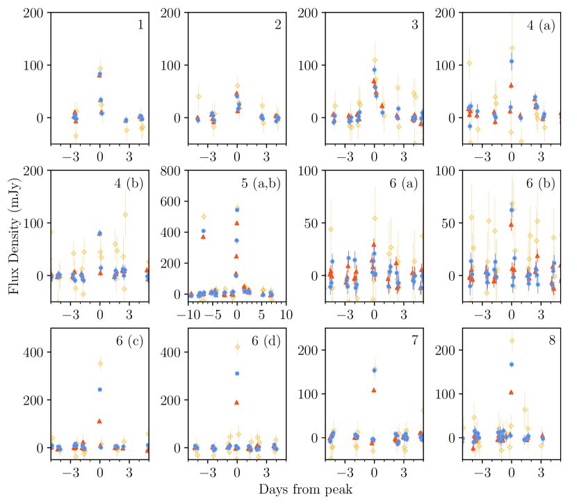
Using computing resources at the South Pole, $0 . ' 25$ -resolution maps are automatically created and filtered following every two-hour subfield observation. We then construct lightcurves stretching back $14\text{\,}\mathrm{d}\mathrm{a}\mathrm{y}\mathrm{s}$ for each pixel in the subfield. Due to the observing cadence outlined in Section 2, lightcurves tend to have 2-3 clustered data points followed by a gap in time, giving rise to the characteristic time coverage seen in Figure 1. We run the flare fitting algorithm on each lightcurve and flag significant events for further analysis. This analysis pipeline allows for flare detection within no more than twelve hours from the flare time, giving us the ability to send out online alerts to recommend follow-up in other bands. The majority of sources described in this article were observed before this online detection system was activated, but were analyzed using the same pipeline after the fact.

When a transient event is detected, we generate polarized flux density lightcurves in order to determine the peak event amplitude, spectral index, and polarization fraction. To estimate the spectral index $\alpha$ , we fit a frequency-dependent flux model $\phi^{b}=\phi^{$150\text{\,}\mathrm{G}\mathrm{H}\mathrm{z}$}(\frac{b}{$150\text{\,}\mathrm{G}\mathrm{H}\mathrm{z}$})^{\alpha}$ to the three bands using a $\chi^{2}$ metric. We marginalize over the $150\text{\,}\mathrm{G}\mathrm{H}\mathrm{z}$ flux density by using the best-fit $\phi^{$150\text{\,}\mathrm{G}\mathrm{H}\mathrm{z}$}$ for each $\alpha$ , and estimate $1\sigma$ confidence intervals using a $\Delta\chi^{2}=1$ criterion. Polarization fractions are estimated from the Stokes- $Q$ and Stokes- $U$ lightcurves using the maximum-likelihood approach of Vaillancourt (2006) to reduce noise bias on the polarized flux density $P=\sqrt{Q^{2}+U^{2}}$ .

3.2 Backgrounds

The sources presented in this paper belong to a small category of emitters that show highly significant events ( $\mathrm{TS}>100$ , corresponding to $>9.7\sigma$ ) and are, with two exceptions, detected in multiple observations, ruling out an origin in an instrumental glitch, satellite pass, or other noise source. At this level of significance, the expected rate of events from Gaussian fluctuations sourced by instrumental and atmospheric noise is below 1 event per million years of observing. False detections may also be caused by non-astrophysical in-band emitters; these are expected to be the dominant noise source at short timescales. The only such contamination we unambiguously detected at this high significance level was thermal emission from weather balloons launched from the South Pole station by the Antarctic Meteorological Research Center (AMRC)¹¹1https://amrc.ssec.wisc.edu and the National Oceanic and Atmospheric Administration (NOAA).²²2https://www.esrl.noaa.gov/gmd/ozwv/ozsondes/spo.html A small fraction of these balloons drifted through the telescope’s field of view shortly after launch. Based on the typical launch cadence and our observing strategy we expect to detect $\mathcal{O}(10)$ such balloons over the course of an observing season. Weather balloons can show up in maps at brightnesses exceeding $1\text{\,}\mathrm{J}\mathrm{y}$ . Typically, their proximity and fast movement creates recognizable extended structure over scales of many arcminutes. Rather than implement a cut on this signal within an observation, we placed a requirement as part of our detection pipeline that sources appear at a signal-to-noise ratio $>3$ and a fixed location in more than one independent observation. This makes the search presented here insensitive to contamination by man-made sources which are not fixed in RA/Dec and rapidly move out of the field, at the cost of reducing sensitivity to rapid events. Two of the 15 detected flares (source 7 and 8) were originally detected by other means, as part of debugging the analysis pipeline, and are included here despite being detected in only one observation. In the case of these two sources, a number of other checks were performed (looking at sub-observation-scale data to ensure the source was stationary for a significant amount of time and cross-checking with balloon launch schedules) to ensure the astrophysical origin of the flare. In the future, we expect to be able to automate both weather balloon detection and sub-observation timescale analysis, and relax the multiple-observation requirement across the board.

4 Results

Refer to caption — Figure 1: Lightcurves of the 13 stellar flares observed in this study at $95\text{\,}\mathrm{G}\mathrm{H}\mathrm{z}$ (red), $150\text{\,}\mathrm{G}\mathrm{H}\mathrm{z}$ (blue), and $220\text{\,}\mathrm{G}\mathrm{H}\mathrm{z}$ (gold). Two of the flares for Z Ind were close in time and are shown together in one panel. In all cases, the rise and fall times are short (hours or less) and the spectra approximately flat.

				Peak Flux Density (mJy)
ID	RA	Dec	Time (UTC)	$95\text{\,}\mathrm{G}\mathrm{H}\mathrm{z}$	$150\text{\,}\mathrm{G}\mathrm{H}\mathrm{z}$	$220\text{\,}\mathrm{G}\mathrm{H}\mathrm{z}$	$\mathrm{TS}$
1	$23 h 20 m 47 . s 6$	$- 67 ° 23 ' 23 ″$	2020-03-26 02:25	$81$ p m 4	$83$ p m 5	$93$ p m 19	709
2	$23 h 13 m 53 . s 1$	$- 68 ° 17 ' 34 ″$	2020-04-01 18:12	$46$ p m 4	$40$ p m 5	$61$ p m 20	213
3	$21 h 01 m 21 . s 2$	$- 49 ° 33 ' 15 ″$	2020-04-02 14:50	$70$ p m 6	$91$ p m 9	$103$ p m 36	541
4 (a)	$21 h 20 m 44 . s 5$	$- 54 ° 37 ' 56 ″$	2020-06-03 02:35	$61$ p m 6	$108$ p m 17	$230$ p m 69
(b)			2020-09-04 09:15	$80$ p m 6	$80$ p m 6	$44$ p m 25	134
5 (a)	$21 h 54 m 23 . s 8$	$- 49 ° 56 ' 36 ″$	2020-06-17 09:20	$370$ p m 6	$408$ p m 7	$501$ p m 28
(b)			2020-06-24 06:09	$459$ p m 6	$543$ p m 8	$558$ p m 30	$16\,416$
6 (a)	$02 h 34 m 22 . s 4$	$- 43 ° 47 ' 53 ″$	2020-06-21 10:42	$29$ p m 6	$21$ p m 7	$54$ p m 30
(b)			2020-07-10 08:24	$48$ p m 6	$62$ p m 7	$68$ p m 27
(c)			2020-09-17 04:51	$111$ p m 6	$243$ p m 8	$352$ p m 32
(d)			2020-11-05 15:34	$189$ p m 6	$310$ p m 8	$422$ p m 33	2715
7	$02 h 55 m 31 . s 6$	$- 57 ° 02 ' 54 ″$	2020-09-18 06:34	$109$ p m 5	$154$ p m 7	$157$ p m 25	1119
8	$00 h 21 m 28 . s 7$	$- 63 ° 51 ' 10 ″$	2020-11-14 01:47	$104$ p m 5	$167$ p m 7	$221$ p m 25	1184
9	$22 h 41 m 16 . s 7$	$- 54 ° 01 ' 07 ″$	2020-07-08	$13$ p m 2	$13$ p m 2	$14$ p m 7	221
10	$03 h 01 m 16 . s 1$	$- 57 ° 19 ' 21 ″$	2020-07-08	$24$ p m 2	$36$ p m 3	$40$ p m 10	1090

Table 1: Transient events detected by SPT-3G between March 23, 2020 and November 15, 2020. Each unique source was given a numbered ID, and each flare was labeled by a letter in the case of multiple flares. Source RA and Dec are the best-fit locations measured by SPT-3G. The horizontal line differentiates the stellar flares (above) from the long-duration, likely extragalactic transients (below). All sources listed have average flux densities below

5\text{\,}\mathrm{m}\mathrm{J}\mathrm{y}

150\text{\,}\mathrm{G}\mathrm{H}\mathrm{z}

in 2019 SPT-3G data. Peak flux densities are averaged over subfield observations and quoted relative to the 2019 average. Peak flare times correspond to the beginning of the subfield observation in the case of stellar flares, and to the center of a week-long integration in the case of the long-duration transients. The test statistic (

\mathrm{TS}

) value is computed on the full 2020 lightcurve for each source and is shown only for the flare that maximizes the

\mathrm{TS}

(generally the brightest one); the cut value used in this search is

TS>100

. Several stars showed other flares that had a signal-to-noise

>5

in at least one observing band and are also shown in this table.

During 3500 hours of observations taken over an 8-month period from 23 March to 15 November, 2020, we observed 10 unique sources with at least one $\mathrm{TS}>100$ event at locations not associated with point sources previously detected by any SPT survey. This was enforced for SPT-3G by masking point sources with an average $150\text{\,}\mathrm{G}\mathrm{H}\mathrm{z}$ flux density greater than $5\text{\,}\mathrm{m}\mathrm{J}\mathrm{y}$ in 2019.

After detecting a source with at least one flare above the $\mathrm{TS}$ threshold, we inspect the lightcurve and tag other flares with signal-to-noise $>5$ in at least one of the observing bands, bringing the total up to the 15 events shown in Table 1. The detected flares have emission timescales ranging from tens of minutes to three weeks, with peak brightnesses (averaged over the $\sim$ 20 minutes of on-source time during the subfield observation) at $150\text{\,}\mathrm{G}\mathrm{H}\mathrm{z}$ from $15\text{\,}\mathrm{m}\mathrm{J}\mathrm{y}540\text{\,}\mathrm{m}\mathrm{J}\mathrm{y}$ , nearing the brightest mm-wave sources in the SPT-3G footprint. Given the upper limit on quiescent flux density in 2019 SPT-3G data of $<5\text{\,}\mathrm{m}\mathrm{J}\mathrm{y}$ for these objects, this represents factors of at least $4100$ increase in luminosity above the sources’ quiescent states.

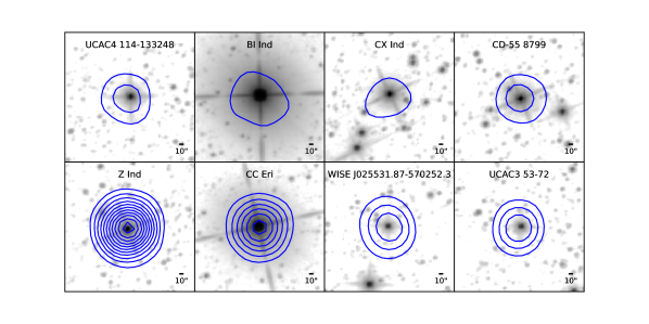
The detected objects are split into two classes. The majority (13 flares from 8 objects) are associated with stars of a wide variety of types (Section 4.1) and reminiscent of a small number of reports in the literature by e.g. Naess et al. (2020); Massi et al. (2006); Brown & Brown (2006) of serendipitously detected mm-wave stellar flares. Stellar flare associations in WISE with SPT-3G flux density contours are shown in Figure 2. The fast timescale of emission (from tens of minutes to hours) and approximately flat spectra are suggestive of synchrotron emission, but the lack of detectable linear polarization and sometimes-rising spectra (Table 2) imply the emission region is likely inhomogeneous or optically thick for at least part of the observing period. The remaining two events are not spatially coincident with any cataloged galactic sources, suggesting an extragalactic origin. These two sources (Section 4.2) had triangular light curves lasting $2\text{\,}\mathrm{w}\mathrm{e}\mathrm{e}\mathrm{k}\mathrm{s}3\text{\,}\mathrm{w}\mathrm{e}\mathrm{e}\mathrm{k}\mathrm{s}$ , with flat spectra and peak flux densities between $15\text{\,}\mathrm{m}\mathrm{J}\mathrm{y}40\text{\,}\mathrm{m}\mathrm{J}\mathrm{y}$ . Due to the high instantaneous signal-to-noise on the short-duration flares, the typical positional uncertainties for these events are $\lesssim$ $10\text{\,}\mathrm{a}\mathrm{r}\mathrm{c}\mathrm{s}\mathrm{e}\mathrm{c}$ , leading to unambiguous associations with known variable stars. Position determination for the two long-duration sources is discussed in more detail in Section 4.2.

		Pol. Frac. (95% UL)
ID	Spectral Index	$95\text{\,}\mathrm{G}\mathrm{H}\mathrm{z}$	$150\text{\,}\mathrm{G}\mathrm{H}\mathrm{z}$
1	$0.10$ p m 0.16	$<0.24$	$<0.20$
2	$-0.1$ p m 0.3	$<0.44$	$<0.37$
3	$0.6$ p m 0.2	$<0.33$	$<0.30$
4 (a)	$1.0$ p m 0.4	$<0.34$	$<0.55$
(b)	$-0.2$ p m 0.2	$<0.33$	$<0.25$
5 (a)	$0.25$ p m 0.05	$<0.06$	$<0.06$
(b)	$0.30$ p m 0.04	$<0.04$	$<0.06$
6 (a)	$-0.4$ p m 0.9	$<0.79$	$<1$
(b)	$0.6$ p m 0.3	$<0.47$	$<0.33$
(c)	$1.52$ p m 0.10	$<0.16$	$<0.11$
(d)	$1.04$ p m 0.07	$<0.12$	$<0.09$
7	$0.71$ p m 0.11	$<0.16$	$<0.14$
8	$1.07$ p m 0.10	$<0.31$	$<0.14$
9	Figure 9	$<0.46$	$<0.59$
10	Figure 9	$<0.31$	$<0.27$

Table 2: Spectral indices and

95\text{\,}\mathrm{\char 37\relax}

upper-limit polarization fractions for the transient events listed in Table 1. No sources had statistically significant detections of polarization. Polarization fractions shown are calculated only at flare peaks.

220\text{\,}\mathrm{G}\mathrm{H}\mathrm{z}

polarization fractions are omitted from this table due to low signal-to-noise.

A large fraction of the flares were in locations covered by the All-Sky Automated Survey for SuperNovae (ASAS-SN, Shappee et al., 2014; Kochanek et al., 2017), which provides optical lightcurves with a daily or near-daily cadence. For two of the stellar flares, we found evidence for optical activity in the ASAS-SN data. Additionally, one of those two was under observation by the Transiting Exoplanet Survey Satellite (TESS, Ricker et al., 2015) at the time of the flare, providing simultaneous mm-wave and optical coverage of an energetic stellar flare with high time resolution. The remaining flares were not associated with optical excesses, and none of the events reported here were coincident with reports to alert systems (GCN³³3https://gcn.gsfc.nasa.gov/ or ATel⁴⁴4http://www.astronomerstelegram.org).

4.1 Stellar flares

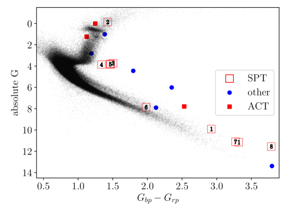
The observed flares arise in a wide variety of stars. The Hertzsprung-Russell (HR) diagram for these stars is shown in Figure 3, using data from the Gaia mission (Gaia Collaboration et al., 2016, 2018). Most of the associated stars are known to be X-ray emitters, with counterparts in the ROSAT All-Sky Survey 2RXS catalog (Boller et al., 2016). Only the two M dwarfs, UCAC3 53-724 and WISE J025531.87-570252.3, are not known X-ray emitters. By selecting on mm-wave flaring in stars, we appear to be highly biased toward stars that are X-ray sources. Coronal activity is related to both flaring and X-ray emission so the correspondence is not unexpected. We randomly selected stars in the SPT-3G footprint with Gaia apparent magnitude G $<$ 15 and found that less than $1\%$ had a 2RXS source within $1 '$ . We also found that the probability of a random point being within $15 ″$ (the furthest SPT-3G flare position association is $13 ″$ ) of a Gaia source of G $<$ 15 within the SPT-3G $1500\text{\,}\deg^{2}$ footprint is $2\times 10^{-3}$ , lending further confidence to the associations.

ID	Association	Distance (pc)	$\nu L_{\nu}^{95}$ ( $\mathrm{erg}\text{\,}{\mathrm{s}}^{-1}$ )	$\nu L_{\nu}^{150}$ ( $\mathrm{erg}\text{\,}{\mathrm{s}}^{-1}$ )	$\nu L_{\nu}^{220}$ ( $\mathrm{erg}\text{\,}{\mathrm{s}}^{-1}$ )	Type
1	UCAC4 114-133248	$41.0$ p m 0.1	$1.6\text{\times}{10}^{28}$	$2.5\text{\times}{10}^{28}$	$4.1\text{\times}{10}^{28}$	Double M Dwarfs^∗
2	BI Ind	$312$ p m 3	$5.1\text{\times}{10}^{29}$	$7.0\text{\times}{10}^{29}$	$1.6\text{\times}{10}^{30}$	RS CVn^∗
3	CX Ind	$235$ p m 3	$4.4\text{\times}{10}^{29}$	$9.0\text{\times}{10}^{29}$	$1.5\text{\times}{10}^{30}$	BY Dra Variable^∗
4 (a)	CD-55 8799	$201$ p m 2	$2.8\text{\times}{10}^{29}$	$7.9\text{\times}{10}^{29}$	$2.5\text{\times}{10}^{30}$	Rotational Variable^∗
(b)			$3.7\text{\times}{10}^{29}$	$5.8\text{\times}{10}^{29}$	$4.7\text{\times}{10}^{29}$
5 (a)	Z Ind	$199$ p m 1	$1.7\text{\times}{10}^{30}$	$2.9\text{\times}{10}^{30}$	$5.2\text{\times}{10}^{30}$	Rotational Variable^∗
(b)			$2.1\text{\times}{10}^{30}$	$3.9\text{\times}{10}^{30}$	$5.8\text{\times}{10}^{30}$
6 (a)	CC Eri	$11.537$ p m 0.005	$4.4\text{\times}{10}^{26}$	$5.0\text{\times}{10}^{26}$	$1.9\text{\times}{10}^{27}$	BY Dra Variable^∗
(b)			$7.3\text{\times}{10}^{26}$	$1.5\text{\times}{10}^{27}$	$2.4\text{\times}{10}^{27}$
(c)			$1.7\text{\times}{10}^{27}$	$5.8\text{\times}{10}^{27}$	$1.2\text{\times}{10}^{28}$
(d)			$2.9\text{\times}{10}^{27}$	$7.4\text{\times}{10}^{27}$	$1.5\text{\times}{10}^{28}$
7	WISE J025531.87-570252.3	$45.6$ p m 0.1	$2.6\text{\times}{10}^{28}$	$5.8\text{\times}{10}^{28}$	$8.6\text{\times}{10}^{28}$	M Dwarf
8	UCAC3 53-724	$43.9$ p m 0.2	$2.3\text{\times}{10}^{28}$	$5.8\text{\times}{10}^{28}$	$1.1\text{\times}{10}^{29}$	M Dwarf

Table 3: Assumed associations of stellar flares and physical properties of events: parallax-based distance, isotropic mm-wave luminosity

\nu L_{\nu}

, and type of star. All sources with types showing an asterisk have 2RXS X-ray sources within

1 ​'

. Distances were pulled from the Gaia DR2 (Gaia Collaboration et al., 2018).

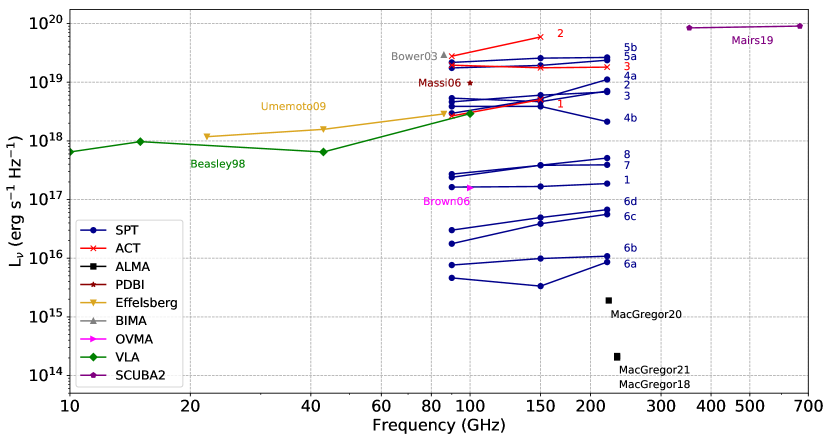
The isotropic mm-wave luminosities $\nu L_{\nu}$ of the flaring events are shown in Table 3 and range from roughly $2\text{\times}{10}^{27}\text{\,}\mathrm{erg}\text{\,}{\mathrm{s}}^{-1}6\text{\times}{10}^{30}\text{\,}\mathrm{erg}\text{\,}{\mathrm{s}}^{-1}$ in the SPT-3G bands. At the bright end, this is comparable to previous mm-wave flares seen in RS CVn stars (Brown & Brown, 2006; Beasley & Bastian, 1998) or T Tauri stars (Massi et al., 2006; Salter et al., 2010; Bower et al., 2003), although not as luminous as the sub-mm flare event in JW 566 (Mairs et al., 2019). The faint flares are brighter than those previously seen at similar wavelengths in M dwarfs (MacGregor et al., 2020). jhe isotropic luminosities per unit frequency $L_{\nu}$ of SPT stellar flares and selected mm-wave flares from the literature are compared in Figure 4.

While the stars have a wide range in properties, there are some themes that emerge. BI Ind (Source 2) is known to be of the type RS CVn and it has been suggested that both CX Ind (Source 3) and CD-55 8799 (Source 4) are RS CVn stars (Berdnikov & Pastukhova, 2008); this classification would be consistent with the similar energetics observed in the flares. BI Ind and the two historical RS CVn flare stars mentioned above are all in the giant branch of the HR diagram; however the possible RS CVn stars CX Ind and CD-55 8799 are redder and lower-luminosity than the typical giant. The flare energy for BI Ind is comparable to the two historical flare stars. Two stars associated with mm-wave flares detected by ACT are also in that part of the HR diagram, with similar flare energy, although these stars have not previously been identified as RS CVn.

Two sources (CX Ind, Source 3 and CC Eri, Source 6) are classified as BY Draconis-type variables in the SIMBAD⁵⁵5http://simbad.u-strasbg.fr/simbad database, as is the previously known flare star AU Mic, which lies very close in the HR diagram to CC Eri. Two other sources are classified as “Rotationally Variable,” but are almost indistinguishable in the HR diagram from CX Ind. In terms of flare energy, CC Eri has substantially lower energy flux than the RS CVn stars, although more than ten times the flux of AU Mic, while CX Ind is energetically comparable to BI Ind. The remaining three stellar flares (Sources 1, 7, and 8) detected in this work are late M dwarfs, with one of them (UCAC4 114-133248, Source 1) actually a pair of M dwarfs. The flare energy flux is comparable in these three cases (few $\times$ $10^{28}\text{\,}\mathrm{erg}\text{\,}{\mathrm{s}}^{-1}$ ), but in all cases at least a thousand times more luminous than the well-known Proxima Centauri mm-wave flare seen by MacGregor et al. (2018).

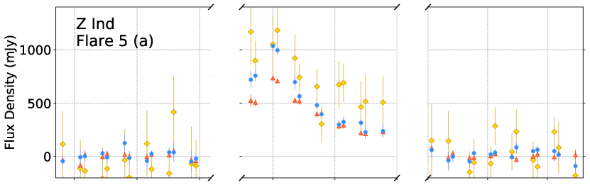
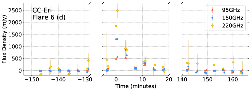
As described in Section 2, the SPT-3G raster scan observing strategy allows a limited ability to observe timescales shorter than 2 hours by examining the individual detector scans over a source position within an observation. There are typically 10 raster scans covering any given point in the subfield, which occur over $\sim$ 20 minutes of the 2-hour observation window. Depending on the right ascension of the source, these rasters are spaced a maximum of 3 minutes apart. A preliminary examination of these data for flare 5(a), associated with Z Ind, and flare 6(d), associated with CC Eri, shows a true peak brightness exceeding $1\text{\,}\mathrm{J}\mathrm{y}$ at $150\text{\,}\mathrm{G}\mathrm{H}\mathrm{z}$ , with emission falling rapidly on 10-minute scales (see Figure 5). Due to the sub-observation timescales of some of these flares, the measured per-observation peak flux density, as reported in Table 1, is below the true peak amplitude. Future analyses may be able to trigger on such sub-observation data and provide a more detailed view of the sky at these minute scales than we present in this publication.

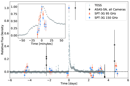
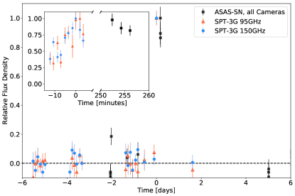
We searched the ASAS-SN variable stars database for optical flux data near the peak times of the stellar flares. Six of the eight stars had some simultaneous ASAS-SN coverage. Of these, two show strong evidence for optical activity related to the millimeter-wave flares detected by SPT-3G: WISE J025531.87-5702523 (Source 7) and UCAC3 53-724 (Source 8), both M Dwarfs. Source 8 has a single ASAS-SN observation consisting of three successive 15-second exposures in V-band, showing a $5\sigma$ increase in flux roughly 4 hours after the observed SPT-3G peak. There are large gaps in both the SPT-3G and ASAS-SN data, and no obvious conclusions can be drawn about the relation between the two detections. Source 7 has one ASAS-SN data point significantly above mean nearly 15 hours after the SPT-3G flare. Serendipitously, TESS had near-continuous coverage of Source 7 in the $600\text{\,}\mathrm{n}\mathrm{m}1000\text{\,}\mathrm{n}\mathrm{m}$ band for the entire duration of the SPT-3G observation, providing high-time-resolution data that shows a bright optical flare beginning some minutes before the first SPT-3G detection and decaying slowly over the next several hours (Brasseur et al., 2019). We show lightcurves for both of the flares with significant optical counterparts in Figure 6. The data from different instruments are rescaled to allow comparison of the time behavior of both sources without making any inference about relative or absolute luminosities. As seen in the TESS data, the optical counterpart to the millimeter-wave flare of Source 7 starts rising an hour before the beginning of SPT-3G coverage. Starting at the first SPT-3G data point, both optical and mm rise rapidly until peaking 10 minutes later. The mm-wave lightcurve quickly falls back to half the observed peak flux before losing coverage, while the optical slowly decays and does not fall back to quiescence until some 24 hours after the peak.

4.2 Extragalactic transients

The two remaining sources are not obviously associated with any galactic source but, at low confidence, may be associated with WISE galaxies. For these two longer-duration sources, the Fermi All-sky Variability Analysis (Abdollahi et al., 2017) shows no significant associated gamma ray flare within several degrees of either source. In addition, no significant optical activity was seen in ASAS-SN for either source. Source positions are determined from the peak of the likelihood surface ( $\mathrm{TS}$ surface) created by applying the transient-finding algorithm to every pixel in a $3 '$ $\times$ $3 '$ box around the source. Statistical positional uncertainties are expected to scale as the ratio of the beam width to signal-to-noise, and are estimated from the width of the $\mathrm{TS}$ surface using $\Delta\mathrm{TS}=2.3$ for a $\chi^{2}$ distribution with $2$ degrees of freedom. To the extent that the flaring lightcurves approximate the Gaussian ansatz for the flare model, the $\mathrm{TS}$ map represents the optimally weighted combination of the different observing bands and periods in order to maximize localization precision. When we apply this method to the stars, where the association is unambiguous, there is an additional variance in position that is consistent with residual pointing uncertainty of $4 . ″ 4$ in addition to the statistical uncertainties in localization. We add this additional uncertainty in quadrature to estimate the position uncertainties, finding sources 9 and 10 to have position uncertainties of $7 . ″ 6$ and $5 . ″ 2$ , respectively, as shown in Figure 7.

Source 9 (SPT-SV J224116.7-540107) is $38 ″$ from a weak ROSAT X-ray emitter 2RXS J224112.8-540103, which has a positional uncertainty of $\sim 21 ″$ (Boller et al., 2016). This X-ray source has been associated with WISEA J224115.38-540102.3 (Salvato et al., 2018), a galaxy that is $12 ″$ from the SPT-3G position. There is another WISE galaxy that is closer, WISEA J224117.10-540105.2, at a separation of only $4 ″$ , but 2 magnitudes fainter in WISE W1 (Band 1, $3.4\text{\,}\mu\mathrm{m}$ ). The larger sky density of such faint galaxies greatly increases the probability of chance alignment, even at this much closer distance. Using the local density of AllWISE sources (Cutri & et al., 2014) within a $1 °$ radius, the probability of a random AllWISE source being brighter and closer than either the dim or bright potential counterpart are $6\text{\,}\mathrm{\char 37\relax}$ and $8\text{\,}\mathrm{\char 37\relax}$ , respectively.

Thus, it is not possible to make a definitive association of source 9 with a cataloged object. Further study will be required to determine the counterpart for this source, for example with ALMA follow-up or detailed SED modeling using multiwavelength data.

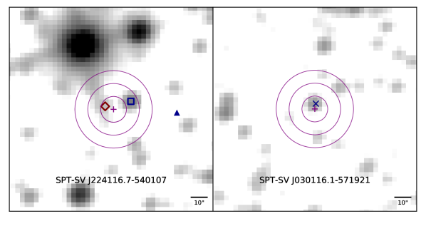
Source 10 (SPT-SV J030116.1-57192) is within $3 ″$ of the galaxy WISEA J030116.15-571917.7, with the next-closest source being $17 ″$ away and substantially fainter (1.4 magnitudes in W1), making this association more secure. The localizations of source 9 and 10 are shown in Figure 7.

The physical mechanism of the transient emission is unknown. It is possible that the events are flares from AGN, which often have flaring behavior on this timescale. A post-detection analysis revealed an average $150\text{\,}\mathrm{G}\mathrm{H}\mathrm{z}$ flux density in 2019 of $4.1\pm 0.6\text{\,}\mathrm{m}\mathrm{J}\mathrm{y}$ and $2.5\pm 0.6\text{\,}\mathrm{m}\mathrm{J}\mathrm{y}$ for source 9 and 10 respectively. The luminosity increase of source 9 from the 2019 average to the peak of the detected flare—a factor of 4—is at the upper limit of what is observed in brighter ( $>10\text{\,}\mathrm{m}\mathrm{J}\mathrm{y}$ ) sources monitored by SPT-3G. Source 10 increased by a factor of 15, which is much larger than what is typical for bright AGN observed by the SPT or by Trippe et al. (2011) in this band (even at the 95% CL lower limit, which is still a factor of 7.4 increase) and may represent an origin different from ordinary AGN flaring or the potential for greater variability in faint AGN at millimeter wavelengths.

There is no cataloged radio source associated with either position, so both would require AGN with flat or rising spectra at radio wavelengths. Radio observations made with the 887 MHz Australian Square Kilometer Array Pathfinder (ASKAP) at points in time before and after the main mm flare of both sources (ASKAP observations on 28/29 March 2020 and 29/30 August 2020) do not show any evidence of either source at a depth of $0.20\text{\,}\mathrm{m}\mathrm{J}\mathrm{y}$ (Hotan et al., 2020). No overlapping ASKAP observations were made during the peak period of June–July 2020. Follow-up observations of these galaxies with deep radio and mm-wave observations may be able to identify possible AGN activity in these sources and shed light on whether the events observed here are part of some continuing flaring behavior from these objects.

The timescales and energies (assuming these sources are at an unremarkable redshift $z\lesssim 1$ ) are also consistent with expectations for tidal disruption events or an object like AT2018cow (Ho et al., 2019), but there were no transient alerts from observations at other wavelengths issued that match these objects.

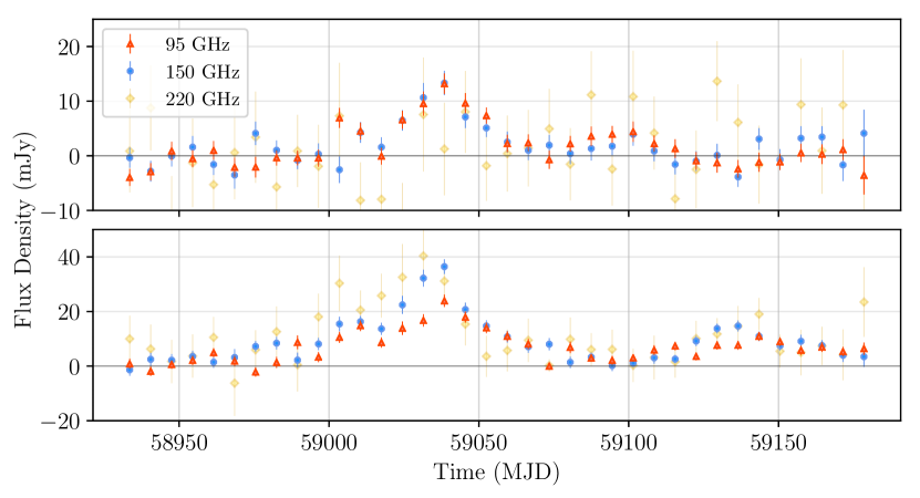
It is perhaps notable that both long-duration transient events, though $35 °$ apart on the sky, rise and fall with similar looking lightcurves and peak in the same week of 2020 (see Figure 8). Given the 36-week observing period this is not an unlikely coincidence. Additionally, most possible sources of systematic contamination can be eliminated by the fact that the two sources sit in different subfields. The center line of the SPT-3G footprint is at $- 56 °$ declination, and the top and bottom half of the field use independent bolometer tunings, different HII calibration sources, and are observed on different observing days. The individual maps that contain the brightest transient observations show no signs of miscalibration, excess noise or excess pointing jitter, and other in-field sources have fluxes consistent with previous and subsequent observations. It is possible that some of the same physics is at play in these two sources to explain the similarity in flare shape and duration; further observations of similar events will provide more information.

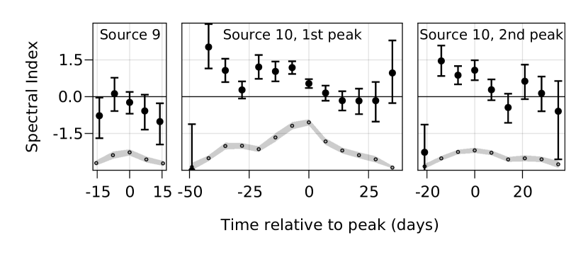
The emission spectrum of Source 10 shows a rising spectrum before the peak of the emission and a flat spectrum thereafter (Figure 9), while the dimmer Source 9 has large spectral uncertainties. This is consistent, though not uniquely so, with a self-absorbed synchrotron spectrum from a young cooling jet, with the initial brightening arising from falling self-absorption more than counteracting the cooling source and the peak of the spectrum moving through SPT-3G’s observing bands at the peak emission time. No linear polarization was detected from the two sources at either the flare peak (Table 2) or when integrating over the flare, the latter approach giving $2\sigma$ polarization fraction upper limits of 0.14, 0.12, and 0.49 at $95\text{\,}\mathrm{G}\mathrm{H}\mathrm{z}150\text{\,}\mathrm{G}\mathrm{H}\mathrm{z}220\text{\,}\mathrm{G}\mathrm{H}\mathrm{z}$ respectively for Source 10, and 0.22 and 0.32 at $95\text{\,}\mathrm{G}\mathrm{H}\mathrm{z}150\text{\,}\mathrm{G}\mathrm{H}\mathrm{z}$ for Source 9. These limits are weak enough that polarization information does not provide strong constraints on the emission mechanism or local magnetic field coherence in the emission region.

5 Discussion and Conclusions

The detection of 15 bright millimeter-wavelength flares in this work, many far above threshold for SPT-3G, suggests that these kinds of flares are common, and that a large number of sources remain to be detected. For example, a naive extrapolation of the rate of stellar flares seen in this paper—the rate of extragalactic transients is too small to draw a robust conclusion—would imply a rate of around a thousand flares of similar brightness per year over the whole sky. Further, the stellar flares seen here are short enough in time (minutes to hours) that many are missed by SPT-3G as a result of our observing cadence and analysis choices for this search. In addition to those missed because we are less sensitive to flares on timescales shorter than a few hours, our observing strategy has day-long gaps between re-observations of each subfield pair (Section 2). This reduces the observing efficiency for hour-scale sources to approximately $23\text{\,}\mathrm{\char 37\relax}$ over our $1500\text{\,}\deg^{2}$ survey, which implies that the true rate of bright stellar flares of the type seen here is at least 4000 per year on the full sky.

The extragalactic transients seen here are more of a puzzle. The emission seen from both sources has a spectrum that evolves from rising to flat or falling, consistent with a newly emitted jet, and both sources show a second, smaller flare days to weeks afterwards. Both sources were convincingly detected (though at low flux density) in the 2019 average map, but it is unclear what emission mechanism(s) caused the extreme flares seen here. One possibility is that these flares were the result of regular AGN activity, but such large ratios of outburst to mean luminosity ( $\sim 4$ and $\sim 15$ for sources 9 and 10, respectively) are rare: Typical SPT-3G AGN fluxes vary by much smaller factors of $\lesssim 50\%$ , with excursions to above 3 observed only in extreme cases (seen in $<1\%$ of SPT-3G sources), and no sources seen with luminosity ratios above 4 when comparing 2020 peak to 2019 average flux data. That sample, however, consists of brighter AGN and might not be representative of the unexplored population of faint AGN.

Such large luminosity variations are not unprecedented, especially over long timescales. The transient source ACT-T J061647-402140⁶⁶6https://www.astronomerstelegram.org/?read=12738, a possible mm-wave counterpart to the transient gamma-ray blazar Fermi 0617-4026, increased in brightness by a similar factor of $\sim 13$ between June 2016 and January 2018. Comparing the ACT flux densities with the 2010-2011 flux densities of the spatially coincident source SPT-S J061647-402147⁷⁷7https://www.astronomerstelegram.org/?read=12837 indicates an increase in flux by a factor of 15-20 over ${\sim}7$ years. The emission seen is also too long in duration to be a GRB afterglow, which typically last for a few days (Ghirlanda et al., 2013). Other possibilities, like a tidal disruption event, cannot be tested with the limited amount of data available.

The SPT-3G camera will continue to observe this $1500\text{\,}\deg^{2}$ footprint until the completion of the survey at the end of 2023. This should at least quadruple the number of detected mm-wave transients with similar brightness, potentially probe new classes of variable mm-wave sources, and discover many more fainter sources as improvements in the analysis increase the sensitivity and time resolution of the search. An already operating online alert system, using the methods described in this article, will soon provide public notice of these detections with latencies of $<24$ hours, enabling multi-wavelength follow-up to determine the nature of the emission seen in this work, as well as characterization of new sources while they are exhibiting variability.

Acknowledgments

The authors thank Anna Ho for helpful comments on a draft version of this paper. We are also grateful to Jeff DeRosa and Johan Booth for providing guidance for South Pole weather balloons. Thanks to Charles Gammie, Leslie Looney, Paul Ricker, Bob Rutledge, and Laura Chomiuk for invaluable early discussions. The South Pole Telescope program is supported by the National Science Foundation (NSF) through grants PLR-1248097 and OPP-1852617, with this analysis and the online transient program supported by grant AST-1716965. Partial support is also provided by the NSF Physics Frontier Center grant PHY-1125897 to the Kavli Institute of Cosmological Physics at the University of Chicago, the Kavli Foundation, and the Gordon and Betty Moore Foundation through grant GBMF#947 to the University of Chicago. Argonne National Laboratory’s work was supported by the U.S. Department of Energy, Office of High Energy Physics, under contract DE-AC02-06CH11357. Work at Fermi National Accelerator Laboratory, a DOE-OS, HEP User Facility managed by the Fermi Research Alliance, LLC, was supported under Contract No. DE-AC02-07CH11359. The Cardiff authors acknowledge support from the UK Science and Technologies Facilities Council (STFC). The IAP authors acknowledge support from the Centre National d’Études Spatiales (CNES). JV acknowledges support from the Sloan Foundation. The Melbourne authors acknowledge support from the Australian Research Council’s Discovery Project scheme (DP200101068). The McGill authors acknowledge funding from the Natural Sciences and Engineering Research Council of Canada, Canadian Institute for Advanced Research, and the Fonds de recherche du Québec Nature et technologies. The UCLA and MSU authors acknowledge support from NSF AST-1716965 and CSSI-1835865. This research was done using resources provided by the Open Science Grid (Pordes et al., 2007; Sfiligoi et al., 2009), which is supported by the NSF award 1148698, and the U.S. Department of Energy’s Office of Science. The data analysis pipeline also uses the scientific python stack (Hunter, 2007; Jones et al., 2001; van der Walt et al., 2011). This work has made use of data from the European Space Agency (ESA) mission Gaia (https://www.cosmos.esa.int/gaia), processed by the Gaia Data Processing and Analysis Consortium (DPAC, https://www.cosmos.esa.int/web/gaia/dpac/consortium). Funding for the DPAC has been provided by national institutions, in particular the institutions participating in the Gaia Multilateral Agreement. This publication makes use of data products from the Wide-field Infrared Survey Explorer, which is a joint project of the University of California, Los Angeles, and the Jet Propulsion Laboratory/California Institute of Technology, and NEOWISE, which is a project of the Jet Propulsion Laboratory/California Institute of Technology. WISE and NEOWISE are funded by the National Aeronautics and Space Administration. This research has made use of the NASA/IPAC Infrared Science Archive, which is operated by the Jet Propulsion Laboratory, California Institute of Technology, under contract with the National Aeronautics and Space Administration. This paper includes data collected by the TESS mission. Funding for the TESS mission is provided by the NASA’s Science Mission Directorate.

References

Abdollahi et al. (2017) Abdollahi, S., Ackermann, M., Ajello, M., et al. 2017, ApJ, 846, 34
Beasley & Bastian (1998) Beasley, A. J., & Bastian, T. S. 1998, in Astronomical Society of the Pacific Conference Series, Vol. 144, IAU Colloq. 164: Radio Emission from Galactic and Extragalactic Compact Sources, ed. J. A. Zensus, G. B. Taylor, & J. M. Wrobel, 321
Bender et al. (2018) Bender, A. N., Ade, P. A. R., Ahmed, Z., et al. 2018, in Proc. SPIE, Vol. 10708, Proc. SPIE, 1070803
Berdnikov & Pastukhova (2008) Berdnikov, L. N., & Pastukhova, E. N. 2008, Peremennye Zvezdy, 28, 9
Boller et al. (2016) Boller, T., Freyberg, M. J., Trümper, J., et al. 2016, A&A, 588, A103
Bower et al. (2003) Bower, G. C., Plambeck, R. L., Bolatto, A., et al. 2003, ApJ, 598, 1140
Brasseur et al. (2019) Brasseur, C. E., Phillip, C., Fleming, S. W., Mullally, S. E., & White, R. L. 2019, Astrocut: Tools for creating cutouts of TESS images
Braun et al. (2010) Braun, J., Baker, M., Dumm, J., et al. 2010, Astroparticle Physics, 33, 175
Brown & Brown (2006) Brown, J. M., & Brown, A. 2006, ApJ, 638, L37
Carlstrom et al. (2011) Carlstrom, J. E., Ade, P. A. R., Aird, K. A., et al. 2011, PASP, 123, 568
Cutri & et al. (2014) Cutri, R. M., & et al. 2014, VizieR Online Data Catalog, II/328
De et al. (2020) De, K., Hankins, M. J., Kasliwal, M. M., et al. 2020, Publications of the Astronomical Society of the Pacific, 132, 025001
Dutcher et al. (2018) Dutcher, D., Ade, P. A. R., Ahmed, Z., et al. 2018, in Proc. SPIE, Vol. 10708, Proc. SPIE, 107081Z
Dutcher et al. (2021) Dutcher, D., Balkenhol, L., Ade, P. A. R., et al. 2021, arXiv e-prints, arXiv:2101.01684
Gaia Collaboration et al. (2016) Gaia Collaboration, Prusti, T., de Bruijne, J. H. J., et al. 2016, A&A, 595, A1
Gaia Collaboration et al. (2018) Gaia Collaboration, Brown, A. G. A., Vallenari, A., et al. 2018, A&A, 616, A1
Ghirlanda et al. (2013) Ghirlanda, G., Salvaterra, R., Burlon, D., et al. 2013, MNRAS, 435, 2543
Ho et al. (2019) Ho, A. Y. Q., Phinney, E. S., Ravi, V., et al. 2019, ApJ, 871, 73
Holder et al. (2019) Holder, G., Berger, E., Bleem, L., et al. 2019, BAAS, 51, 331
Hotan et al. (2020) Hotan, A., McConnell, D., Whiting, M., & Huynh, M. 2020, ASKAP Data Products for Project AS110 (The Rapid ASKAP Continuum Survey) catalogues. v1. CSIRO. Data Collection.
Hunter (2007) Hunter, J. D. 2007, Computing In Science & Engineering, 9, 90
Jones et al. (2001) Jones, E., Oliphant, T., Peterson, P., et al. 2001, SciPy: Open source scientific tools for Python, [Online; accessed 2014-10-22]
Kochanek et al. (2017) Kochanek, C. S., Shappee, B. J., Stanek, K. Z., et al. 2017, PASP, 129, 104502
Lacy et al. (2020) Lacy, M., Baum, S. A., Chandler, C. J., et al. 2020, Publications of the Astronomical Society of the Pacific, 132, 035001
Lang (2014) Lang, D. 2014, The Astronomical Journal, 147, 108
Law et al. (2018) Law, C. J., Gaensler, B. M., Metzger, B. D., Ofek, E. O., & Sironi, L. 2018, The Astrophysical Journal, 866, L22
MacGregor et al. (2020) MacGregor, M. A., Osten, R. A., & Hughes, A. M. 2020, arXiv e-prints, arXiv:2001.10546
MacGregor et al. (2018) MacGregor, M. A., Weinberger, A. J., Wilner, D. J., Kowalski, A. F., & Cranmer, S. R. 2018, ApJ, 855, L2
MacGregor et al. (2021) MacGregor, M. A., Weinberger, A. J., Loyd, R. O. P., et al. 2021, ApJ, 911, L25
Mairs et al. (2019) Mairs, S., Lalchand, B., Bower, G. C., et al. 2019, ApJ, 871, 72
Massi et al. (2006) Massi, M., Forbrich, J., Menten, K. M., et al. 2006, A&A, 453, 959
Metzger et al. (2015) Metzger, B. D., Williams, P. K. G., & Berger, E. 2015, ApJ, 806, 224
Mooley et al. (2016) Mooley, K. P., Hallinan, G., Bourke, S., et al. 2016, The Astrophysical Journal, 818, 105
Naess et al. (2020) Naess, S., Battaglia, N., Bond, J. R., et al. 2020, arXiv e-prints, arXiv:2012.14347
Pordes et al. (2007) Pordes, R., et al. 2007, J. Phys. Conf. Ser., 78, 012057
Ricker et al. (2015) Ricker, G. R., Winn, J. N., Vanderspek, R., et al. 2015, Journal of Astronomical Telescopes, Instruments, and Systems, 1, 014003
Salter et al. (2010) Salter, D. M., Kóspál, Á., Getman, K. V., et al. 2010, A&A, 521, A32
Salvato et al. (2018) Salvato, M., Buchner, J., Budavári, T., et al. 2018, MNRAS, 473, 4937
Sfiligoi et al. (2009) Sfiligoi, I., Bradley, D. C., Holzman, B., et al. 2009, in 2, Vol. 2, 2009 WRI World Congress on Computer Science and Information Engineering, 428
Shappee et al. (2014) Shappee, B. J., Prieto, J. L., Grupe, D., et al. 2014, ApJ, 788, 48
Trippe et al. (2011) Trippe, S., Krips, M., Piétu, V., et al. 2011, A&A, 533, A97
Umemoto et al. (2009) Umemoto, T., Saito, M., Nakanishi, K., Kuno, N., & Tsuboi, M. 2009, Astronomical Society of the Pacific Conference Series, Vol. 402, ed. Y. Hagiwara, E. Fomalont, M. Tsuboi, and M. Yasuhiro, 400
Vaillancourt (2006) Vaillancourt, J. E. 2006, PASP, 118, 1340
van der Walt et al. (2011) van der Walt, S., Colbert, S., & Varoquaux, G. 2011, Computing in Science Engineering, 13, 22
Whitehorn et al. (2016) Whitehorn, N., Natoli, T., Ade, P. A. R., et al. 2016, ApJ, 830, 143