Automatic Speaker Independent Dysarthric Speech Intelligibility Assessment System

Abstract

Dysarthria is a condition which hampers the ability of an individual to control the muscles that play a major role in speech delivery. The loss of fine control over muscles that assist the movement of lips, vocal chords, tongue and diaphragm results in abnormal speech delivery. One can assess the severity level of dysarthria by analyzing the intelligibility of speech spoken by an individual. Continuous intelligibility assessment helps speech language pathologists not only study the impact of medication but also allows them to plan personalized therapy. It helps the clinicians immensely if the intelligibility assessment system is reliable, automatic, simple for (a) patients to undergo and (b) clinicians to interpret. Lack of availability of dysarthric data has resulted in development of speaker dependent automatic intelligibility assessment systems which requires patients to speak a large number of utterances. In this paper, we propose (a) a cost minimization procedure to select an optimal (small) number of utterances that need to be spoken by the dysarthric patient, (b) four different speaker independent intelligibility assessment systems which require the patient to speak a small number of words, and (c) the assessment score is close to the perceptual score that the Speech Language Pathologist (SLP) can relate to. The need for small number of utterances to be spoken by the patient and the score being relatable to the SLP benefits both the dysarthric patient and the clinician from usability perspective.

url]www.tcs.com

1 Introduction

Dysarthria is a condition which hampers the ability of a person to control the muscles that play a major role in speech delivery. The loss of fine control over muscles that assist the movement of lips, vocal chords, tongue and diaphragm results in abnormal speech delivery. Among other things, this condition affects verbal communication because of hampered intelligibility of spoken speech.

It is believed that $7$ of the $12$ cranial nerves, which perform the task of sending sensory and motor information to all the muscles of the body, are related to speech and language. Damage to any of these nerves can result in hampering control of muscles that assist in speech production [1]. Generally dysarthria is a result of a disease or a stroke that affects the nervous system and not a disease in itself. The speech production is a complex mix of respiration, phonation, resonance, articulation, and prosody. If any of these speech process is affected because of lack of muscle control speech production suffers. Depending on the degree of loss of control over the muscles that assist in articulation dysarthria can range from mild where a person sounds as good as a healthy speaker to severe where it might be very difficult for a listener to understand what is being spoken. There are $6$ types of dysarthria, namely, (a) Ataxic, (b) Flaccid, (c) Hyperkinetic, (d) Hypokinetic, (e) Spastic and (f) Mixed (a mix of Flaccid and Spastic dysarthria).

Table 1: Causes for Different Dysarthria [1].

	Dysarthria Type
Possible Causes	Ataxic	Flaccid	Hyperkinetic	Hypokinetic	Mixed	Spastic
Stroke (Cerebro Vascular Accident)	✓	✓	✓		✓	✓
Trauma	✓	✓			✓	✓
Tumor	✓	✓	✓			✓
Congenital conditions	✓	✓				✓
Infection	✓					✓
Amyotrophic lateral sclerosis					✓
Athetosis			✓
Ballism			✓
Chorea Infection			✓
Drug-induced Dyskinesia			✓
Dystonia			✓
Gilles de la Tourette’s syndrome			✓
Palsies		✓
Parkinsonism Drug-induced				✓
Toxic effects	✓
Viral Infection		✓

The cause for different types of dysarthria is well studied in literature [1]. As seen in Table 1, cerebrovascular accident (CVA), commonly also known as stroke, can result in any kind of dysarthria except, Hypokinetic dysarthria, whereas drug induced Parkinsonism can only cause Hypokinetic dysarthria. Trauma and Tumor can also result in a variety of dysarthria types (see Table 1). While Toxic effects can only induce Ataxia, Viral Infection causes Flaccid dysarthria, diseases like Athetosis, Ballism, Chorea Infection, Drug-induced Dyskinesia, Dystonia and Gilles de la Tourette’s syndrome are known to result in Hyperkinetic dysarthria.

Table 2: Different Dysarthria effecting Speech Characteristics [1].

	Dysarthria Type
Speech Characteristics	Ataxic	Flaccid	Hyperkinetic	Hypokinetic	Mixed	Spastic
Imprecise consonants	✓	✓	✓	✓	✓	✓
Monopitch		✓	✓	✓	✓	✓
Monocloudness			✓	✓	✓	✓
Distorted vowels	✓		✓		✓
Harsh voice (quality)	✓		✓	✓	✓	✓
Hypernasality		✓			✓	✓
Excess and equal stress	✓				✓
Irregular articulatory breakdowns	✓		✓
Low pitch					✓	✓
Reduced stress				✓		✓
Short phrases					✓	✓
Slow rate					✓	✓
Strained-strangled voice			✓			✓
Breathy voice		✓		✓
Inappropriate silences				✓
Loudness control problems	✓
Nasal emission		✓
Prolonged intervals					✓
Short rushes of speech				✓
Variable nasality	✓

A comprehensive mapping between different types of dysarthria and the speech characteristics in shown in Table 2. Out of the 20 speech characteristics, the inability to precisely articulate consonants is a prime characteristic across all types of dysarthria. One of the prime speech characteristic, across all type of dysarthria is the inability to articulate consonants precisely (see Table 2). As can also be seen multiple speech characteristics are visible in a particular type of dysarthria. Clearly a combination of these speech characteristics make the speech of a dysarthric patient unintelligible. The speech characteristics become increasingly visible, rather audible, as dysarthria becomes more profound in a patient. For example, the degree of distortion of a vowel (”vowel distortion”) becomes more profound as dysarthria progresses from mild to severe in case of Ataxic and Hyperkinetic dysarthria. In case of Mixed dysarthria, there is an increase in ”Prolonged interval” between the words or phonemes in spontaneous speech when severity level of dysarthria increases thus, further degrading the intelligibility.

Some of the noticeable characteristics of dysarthria are (a) there is never an island of clear speech, the speech errors are seen uniformly along the entire speech utterance, (b) articulation error is caused due to distortions and deletions, and not the insertion of phonemes, (c) pronunciation of consonants are consistently imprecise, (d) vowels are neutralized, (e) the speech delivery rate is slow and labored and (f) any word requiring large articulatory movement due to complexity in pronunciation results in a decreased articulatory performance.

A speech language therapist (SLP) who specializes in speech therapy can help a person with dysarthria improve speech delivery through medication and practice of suitable exercises to regain control over the articulators. However, this requires an accurate assessment of the degree of dysarthria at the time of diagnosis and during therapy, to understand the effect of medication.

Instrumental investigation for example, using a water manometer fitted with a bleed valve (to measure sub-glottal air pressure), laryngograph (measure abnormalities of closure), electropalatography (tongue movement), pneumotachography (to measure differentials of nasal and oral air flow) [2] are supplemented by perceptual (human) assessment and in many cases, due to lack of instruments, perceptual assessment might be the only possible means of evaluation possible. Perceptual assessment by a trained SLP is considered the gold standard even if we were not to consider the fact that instrumentation based approach are invasive, expensive and painful.

Several tests and metrics developed over the years are used by the SLPs. Three frequently used tests for evaluating dysarthric speech are (a) Assessment of Intelligibility of Dysarthric Speech [3], (b) Frenchay Dysarthria Assessment [4], and (c) Quick Assessment for Dysarthria [5]. While Hoehn and Yahr scale [6], Unified Parkinson’s Disease Rating Scale (UPDRS) [7], and Scale for Assessment and Rating of Ataxia (SARA) [8] are frequently used to measure the severity of dysarthria. All these metrics are influenced by the type of stimuli used to elicit a phonetic utterance [9]. For example, the assessment of speech part of the UPDRS has a scale between $0$ and $4$, where $0$ is normal and a score of $4$ suggests that the speaker is unintelligible most of the time. As seen in Table 3 the interpretation of mildly, moderately, severely are not only SLP (evaluator) dependent but, more importantly, these interpretations have a bearing on the stimuli used to elicit speech from the patient.

Table 3: UPDRS for Speech Intelligibility Assessment [10]. The underlined words are subject to human interpretation.

UPDRS	Interpretation
0	Normal
1	Mildly affected. No difficulty being understood.
2	Moderately affected. Sometimes asked to repeat statements.
3	Severely affected. Frequently asked to repeat statements.
4	Unintelligible most of the time.

Both objective assessment using instruments and perceptual assessment by clinicians show drawbacks. As a result, the research focus is on using signal processing and machine learning (ML) approaches to automatically assess dysarthric speech intelligibility. In this paper we concentrate on automatic dysarthria speech intelligibility assessment. This paper consolidates our work reported in [11], [12] and [13] and expands on it in the following way, (a) we propose two additional new methods to robustly compute the speech intelligibility of the speaker, (b) we derive using visible speech the characteristics of words that make them useful to be used for speech intelligibility characterization, (c) we propose a method to enable selection of an optimal number of words that are sufficient for intelligibility assessment for a language from a set of dictionary words (vocabulary) without affecting the correctness of the assessed intelligibility score. The rest of the paper is organized as follows, in Section 2 we review the existing literature on intelligibility assessment techniques elaborating on the perceptual, instrumental and automatic intelligibility assessment techniques. We describe the proposed intelligibility assessment techniques in Section 3 and also describe the method to derive an optimal set of words from a set of dictionary words in Section 4. The experimental setup is described in Section 5 and we conclude in Section 6.

2 Review of Intelligibility Assessment Methods

The approaches adopted in literature for speech intelligibility assessment can be classified into three broad categories, namely, (a) physiological assessment using sophisticated instruments, (b) perceptual assessment performed by a trained clinician, and (c) automatic speech intelligibility assessment using advancement in signal processing and ML.

The current research focus as well as the thrust of this paper is on the use of automatic methods for dysarthric speech intelligibility assessment. We carry out a brief survey of the existing techniques and not review the perceptual or instrument based assessment techniques.

The advancement in signal processing and ML literature has encouraged researchers to explore the use of signal processing and ML techniques for automatic speech intelligibility assessment. Broadly, these methods aim at measuring the abnormalities in spoken speech by extracting handcrafted acoustic features based on statistical signal processing [14, 15] and/or supervised methods based on ML [16, 17]. Such techniques offer the advantage of frequent, cost effective and objective assessment of speech intelligibility. However, a speech signal is abundant in layered information such as gender, speaker traits, emotion of the speaker in addition to the linguistic content of the speech [18]. These multiple layers (who spoke, how they spoke, what they spoke) of information in the same speech sample makes it difficult to extract features that carry only pathology-specific information. Additionally, the ML models are prone to overfitting during training because of the small corpus size of the disease-specific speech. This makes these models ineffective in terms of generalization over a larger population. One set of such approaches aims at categorizing the patients speech recording into broad categories such as $\{{\tt healthy},{\tt dysarthric}\}$ ($2$ classes) [19, 20] or $\{{\tt high},{\tt medium},{\tt low}\}$ Intelligibility ($3$ classes) rather than providing an absolute intelligibility assessment score. However, a mechanism that can provide continuous intelligibility ratings is of more use in a clinical setting especially, when the assessment scores are synchronous with the perceptual scores understood by the SLP. Subsequently, a set of approaches aimed at learning continuous intelligibility assessment scores have been been researched. Literature in this area can be broadly categorized into (a) reference-free and (b) reference-based approaches.

2.1 Reference-free approaches

Reference-free approaches aim at measuring speech intelligibility without using any prior knowledge associated with healthy or intelligible speech as reference. Different handcrafted features that are believed to be correlated with speech intelligibility have been explored to (a) classify different types of dysarthria (Table 2) (b) assess intelligibility of speech especially that affected by dysarthria.

Phonation features that describe pathological voice such as fundamental frequency $F_{0}$ and jitter have been found useful in quantification of voice tremor [21, 22]. Pitch Period Entropy based assessment was proposed [23] in order to overcome the gender and acoustic environment dependency of these features. Short-time energy and variation of energy (shimmer) [24] have also been effectively used to describe hypophonia. Teager-Kaiser Energy Operator [25], a measure of instantaneous speech intensity, has been used in order to take signal frequency into account. Features that capture energy distribution in power spectra such as Median of Power Spectral Density (MPSD) [26] and Low Short-Time Energy Ratio (LSTER) [27] have also been explored in literature. Acoustic cues based on first three formants, and their corresponding bandwidths can be observed to study the impact on articulatory dynamics, thereby proving to be helpful in estimation of speech intelligibility [28]. Vowel Space Area (VSA) for studying speech intelligibility [29, 30] has also been explored.

An approach for discriminating dysarthric speech from healthy speech by using a set of glottal and openSMILE features have been explored using Support Vector Machine classifier [31]. An investigation of analytic phase features, extracted from the speech signal, by using single frequency filtering technique was performed in [32]. Audio descriptor features used for defining Timbre of musical instruments along with Artificial Neural Network (ANN) model was used in [33] to classify severity levels of dysarthric speech. Multi-tapered spectral estimation to obtain the audio descriptor features was employed for dysarthria classification. A multi-task learning technique to jointly solve dysarthria detection and speech reconstruction tasks was explored by encoding dysarthric speech to a lower dimensional latent space in [34]. Speech rate, pauses, fillers, and Goodness of Pronunciation (GoP) were used as discriminating features to differentiate healthy controls (HC) from individuals with Huntington disease using Long Short Term Memory - Recurrent Neural Network (LSTM-RNN) and Deep Neural Network (DNN) [35]. Classification of patients with Amyotrophic Lateral Sclerosis (ALS), Parkinsons Disease (PD), and Healthy Control (HC) using a Convolutional Neural Network - Long Short Term Memory (CNN-LSTM) based transfer learning framework was proposed in [36]. Dysarthria detection in Mandarin speaking individuals was proposed in [37] using a RNN-LSTM based framework directly on raw speech waveforms. Variations of CNN architecture such as time-CNN, frequency-CNN and tf-CNN to capture spectro-temporal variations in speech of individuals suffering from dysarthria was explored in [38]. The performance of Bi-directional LSTM (BiLSTM) with log-filterbank, Mel-filter Cepstral Coefficients (MFCCs) and i-vector features as input to classify Dutch and English speakers into intelligible and non-intelligible categories was explored in [39]. CNN for automatic early detection of ALS from highly intelligible speech was attempted in [40]. The use of features based on occurrence of $<$unk$>$ token in DeepSpeech, an end-to-end speech-to-alphabet system based on the CTC loss function was effectively employed in [12] in order to achieve a $4$-class classification of different intelligibility levels of dysarthria.

These reference-free methods rely on supervised learning and are usually trained on a small dataset. Due to the size of pathological speech corpora (low resource), they are likely to overfit the train data, thus not performing very well on the test (unseen during training) dataset. In order to tackle this situation, more recently, several reference-based approaches have been proposed.

2.2 Reference-based approaches

The family of reference-based or non-blind approaches involve the use of healthy reference signals in a wide variety of ways. The reference speech signals are used to train systems for example, Automatic Speech Recognition (ASR) engines, which are then employed for evaluating pathological speech to estimate their intelligibility with respect to the healthy speech.

A single speaker-independent Gaussian Mixture Model (GMM) is trained on the data of healthy speakers to create a healthy reference model in [41]. The reference GMM is adapted using pathological speech to generate a GMM-based supervector (feature) to represent the pathological speech signal. The intelligibility score is then obtained by training a regression model on the GMM-based supervector. A total variability subspace modeled by factor analysis method was adopted to assess dysarthria intelligibility in [42]. Acoustic information corresponding to each speech recording was represented by an i-vector and a support vector regression model was trained for intelligibility score estimation. A very similar approach of using i-vector for regression task has been adopted in both [43] and [44]. GMM and DNN based models trained using MFCC features were employed for the task of hypernasality estimation in [45]. Two acoustic models trained on a large corpus of healthy speech, one to measure the nasal resonance from voiced sounds and another to measure the articulatory imprecision from unvoiced sounds was used in [46] to estimate hypernasality in dysarthric subjects.

A phonological feature extractor trained using healthy speech samples was employed to compute statistical phonological characteristics of a speaker using frame-level phonological features in [47]. Similarly, a study was carried out in [48] to understand if ML models trained on normal healthy speech can be adapted to train using pathological speech.

Another set of reference-based approaches are based on training an ASR system using healthy reference speech. The ASR system replaces a human listener and pathological speech intelligibility is computed based on the word error recognition rate. Such an approach has been applied to measure intelligibility of tracheoesophageal speech [49], speech of oral cancer patients [50], head and neck cancer patients [51], and intelligibility of substitute speech after laryngectomy [52].

More recently a short-time objective intelligibility (STOI) approach was proposed in [53]. First utterance-dependent reference signal from multiple healthy speakers was constructed using Dynamic Time Warping (DTW). This reference and the pathological speech (corresponding to the same utterance) was aligned to compute the short-time or spectral cross-correlation. This method, called P-STOI, was evaluated on French and English speakers. Subsequently in [53], an improvised method was proposed which used synthetic speech generated by a text-to-speech (TTS) systems to create a reference speech signal. Spectral bases of the octave band representations of speech was exploited in [54] by first finding subspaces of spectral patterns characterizing intelligible (healthy) and pathological speech using Principal Component Analysis (PCA) or Approximate Joint Diagonalization (AJD) and then measuring the Grassman distance between the two subspaces.

While the automatic speech intelligibility of pathological speech has attracted a lot of attention leading to a researchers trying out different approaches, the main constraint has been in terms of the size of the database, which is often very small and because of privacy issues often not available for use by other groups.

3 Proposed Intelligibility Assessment Approaches

We describe two approaches, one based on high level descriptors extracted directly from speech utterances and the other based on the output of an end-to-end speech to alphabet (S2A) recognition engine, to assess the intelligibility of dysarthric speech. We describe them in detail.

3.1 High Level Descriptors based Intelligibility Assessment

The openSMILE toolkit [55] is an open-source toolkit, used for extraction of features from audio signals. OpenSMILE features have been popularly used for detection of emotions in audio [56], speaker biometric, and detection of voice pathologies [57]. We use the Interspeech 2009 Emotion Challenge configuration [58] to obtain a set of $384$ features corresponding to an input speech signal. Thus, a speech signal can be represented as a $384$ dimensional vector ($F$). Further we normalize $F$ along each of the $384$ dimensions so that the feature value is in the range $(0,1)$.

Let, ${\vec{F}}^{k}(w)$ denote the normalized high level descriptors (feature vector) of length $|F|=384$ corresponding to the Speaker $k$. Note that

$$E(\delta,\eta,w)={{\frac{1}{|F|}}}\sqrt{\sum_{i=1}^{|F|}\left({\vec{F}}_{i}^{\eta}(w)-{\vec{F}}_{i}^{\delta}(w)\right)^{2}}$$

is the Euclidean distance between speaker $\delta$ and speaker $\eta$ speaking the same word $w$ (note that $E(\delta,\eta,w)$ takes a value between $(0,1)$). Then, the intelligibility measure of speaker $d$ speaking the word $w$, denoted by $I_{os}(d,w)$ can be computed as

$$I_{os}(d,w)=\frac{1}{N_{h}}\sum_{l=1}^{N_{h}}E(d,l,w)$$

where $N_{h}$ denotes the number of healthy speakers available in the dataset. Note that $I_{os}(d,w)$ captures the average distance of the speaker $d$ speaking the word $w$ from all the $N_{h}$ healthy speakers who speak the same word $w$. The overall intelligibility of the speaker $d$ across all the words in the dataset can be computed as

$$I_{os}(d)=\frac{1}{|W|}\sum_{w\in W}I_{os}(d,w)$$ (1)

where $W$ is the set of words and $|W|$ is the total number of words in the database. A large value of intelligibility measure $I_{os}(d)$ would mean a larger distance between the speaker $d$ and the healthy speakers in the high level descriptors space. We can easily see that the metric $I_{os}$ is negatively correlated with the perceptually assessed intelligibility score and this is clearly seen in our experimental results.

3.2 Speech to Alphabet (DeepSpeech) based Intelligibility Assessment

Mozilla’s DeepSpeech [59] (DeepSpeech) is an end-to-end deep learning model that converts speech into alphabets based on the Connectionist Temporal Classification (CTC) loss function. The $6$ layer deep model is pre-trained on $1000$ hours of speech from the Librispeech corpus [60]. All the layers, except the $4^{th}$ layer, which has recurrent units, have feedforward dense units. A speech utterance $x$ is segmented into $T$ frames, as is common in speech processing, namely, $x_{t}\ \ \forall t\in\left[0,T-1\right]$. Each frame $x_{t}$ is represented by $26$ MFCCs, namely, $\vec{f}_{t}$. Subsequently the speech utterance $x$ can be represented as a sequence of speech features, namely, $\{\vec{f}_{t}\}_{t=0}^{T-1}$. The input to the DeepSpeech is the speech features from $9$ preceding and $9$ succeeding frames, namely $\{\vec{f}_{t-9}\cdots\vec{f}_{t+9}\}$. The output of the DeepSpeech model is a probability distribution over the alphabet set ${\cal A}$ of a particular language. In case of English language, ${\cal A}=(a,b,\cdots,z,\square,\star,<{\tt unk}>)$ and $|{\cal A}|=29$. Note that there are three additional outputs, namely, $<$unk$>$, $\square$, and $\star$ corresponding to unknown, space and an apostrophe respectively in the alphabet set in addition to the $26$ known English letters. The output at each frame/timestep, $t$ is

$$c^{*}_{t}=\max_{\forall k\in{\cal A}}P\left(\left(c_{t}=k\right)|\left\{\vec{f}_{t-9},\cdots,\vec{f}_{t},\cdots,\vec{f}_{t+9}\right\}\right)$$ (2)

where $c^{*}_{t}\in{\cal A}$. It is important to note that a typical speech recognition engine is assisted by a statistical language model (LM) which helps in masking small acoustic mispronunciations. However as seen in (2) there is no role of LM. This, as we will see later, is vital to speech intelligibility estimation.

Let us define four string operations, namely, (a) ${\cal C}(s,p)$ which counts the number of patterns $p\in{\cal A}$ in the string $s$, (b) ${\cal L}(s)$ is the length of the string $s$, (c) ${\cal S}(s)$ which compresses the string $s$ so that all repetitions are deleted and (d) ${\cal D}(s,p)$ which deletes all the patterns $p\in{\cal A}$ in the string $s$. The string $s$ is typically the output of (2). Table 4 shows some examples of these operation on the output of DeepSpeech string $s$. While we will not be making use of these properties in this paper, it is interesting to note that (a) the order of ${\cal S}$ and ${\cal D}$ does not matter and (b) ${\cal S}^{n}={\cal S}$ and ${\cal D}^{n}={\cal D}$ (see Table 4).

Table 4: Example operation on the output of DeepSpeech.

$s=[$ n a a $\square$ t t t $<$unk$>$ u u u $\square$ r r r r $<$unk$>$ e e $<$unk$>$ $]$
${\cal C}(s,<{\tt unk}>)=$	$3$
${\cal L}(s)=$	$20$
${\cal S}(s)=$	$[$ n a $\square$ t $<$unk$>$ u $\square$ r  $<$unk$>$ e $<$unk$>$ $]$
${\cal D}(s,<{\tt unk}>)=$	$[$ n a a $\square$ t t t u u u $\square$ r r r r e e $]$
${\cal S}({\cal D}({\cal D}(s,<{\tt unk}>),\square))=$	$[$ n a t  u  r  e $]$
${\cal S}({\cal D}({\cal D}(s,\square),<{\tt unk}>))=$	$[$ n a t  u  r  e $]$
${\cal D}({\cal D}({\cal S}(s),\square),<{\tt unk}>)=$	$[$ n a t  u  r  e $]$
${\cal D}({\cal S}({\cal D}(s,\square),<{\tt unk}>))=$	$[$ n a t  u  r  e $]$
${\cal S}^{n}(s)=$	${\cal S}(s)$
${\cal D}^{2}(s,p)\stackrel{{\scriptstyle\Delta}}{{=}}{\cal D}({\cal D}(s,p),p)=$	${\cal D}(s,p)$

In order to estimate the intelligibility, for a given spoken word, $u$, we get the output $c^{*}_{t}$ from (2) for each time step $t$. Let $c^{*}=c^{*}_{1},c^{*}_{2},\cdots$ denote the output sequence for the spoken word $u$. We compute the similarity between $s_{1}={\cal D}({\cal S}(c^{*}),<{\tt unk}>)$ of length $l_{1}=L(s_{1})$ and the ground truth (say $s_{1g}$ of length $l_{g}={\cal L}(s_{1g})$). Note that the operations ${\cal S}$ and ${\cal D}$ are not applicable on the ground truth. The higher the similarity between the two strings ($s_{1}$ and $s_{1g}$) the higher the intelligibility of the utterance $u$. We experiment with three string comparison metrics, namely, (a) Sequence Matcher, (b) Levenshtein distance and (c) occurrence of $<$unk$>$ for computing the intelligibility scores.

Intelligibility based on Sequence Matcher: Sequence matcher is an extension of the Gestalt Pattern Matching algorithm [61]. The similarity between two strings is computed as the number of characters in the matching subsequences divided by the total number of characters in both the strings. The number of matching characters is the length of the longest matching (contiguous) subsequence between the two input strings $s_{1}$ and $s_{1g}$. The intelligibility using the Sequence Matcher technique can be computed as

$$I_{sm}(s_{1},s_{1g})=100*\left(\frac{2*m}{l_{1}+l_{g}}\right)$$ (3)

where $m$ denotes the total number of characters in matching subsequences between $s_{1}$ and $s_{1g}$.

Intelligibility based on Levenshtein Distance: Levenshtein or Edit distance expresses the number of edits (insertions, deletions, substitutions) necessary to convert one sequence to another. The lesser the number of edits the higher is the similarity between the two sequences. The intelligibility using the Levenshtein distance is computed as,

$$I_{ld}(s_{1},s_{1g})=\left(1-\frac{l}{l_{1}+l_{g}}\right)*100$$ (4)

where $l$ represents the edit distance between $s_{1}$ and $s_{1g}$.

Intelligibility Assessment based on $<$unk$>$: The DeepSpeech speech to character has been, like most automatic speech recognition engines, trained on only healthy speech and it is natural that it fails to recognize sounds in pathological speech, an effect of this is the production of the character $<$unk$>$ in (2). Intelligibility of the speech can be estimated from the number of times $<$unk$>$ occurs in the output, namely in $s_{1}$. The intelligibility using this metric is computed as,

$$I_{<{\tt unk}>}(s_{1},s_{1g})=\left(1-\min\left(\frac{{\cal C}(s_{1},<{\tt unk}>)}{{\cal L}(s_{1g})},1\right)\right){{*100}}$$ (5)

where $\min(a,1)$ outputs $1$ when $a\geq 1$, else it outputs the vale of $a$.

So given a set of $w\in W$ words, the patient to be assessed is asked to speak all the $|W|$ words in $W$; the intelligibility score for the patient is then computed as

$${{I_{ld}=}}\frac{1}{|W|}\sum_{i=1}^{|W|}I_{sm}(s_{i},s_{ig});$$ (6)

for Intelligibility based on Sequence Matcher,

$${{I_{sm}=}}\frac{1}{|W|}\sum_{i=1}^{|W|}I_{ld}(s_{i},s_{ig});$$ (7)

for Intelligibility based on Levenshtein Distance and

$${{I_{<{\tt unk}>}=}}\frac{1}{|W|}\sum_{i=1}^{|W|}I_{<{\tt unk}>}(s_{i},s_{ig})$$ (8)

for Intelligibility based on occurrence of $<$unk$>$. Note that all these metrics for intelligibility assessment work, as will be shown in our experiments, independent of the speaker.

Clearly the larger the number of words ($|W|$) that the patient needs to speak the more reliable is the intelligibility score, however a large set of words makes the assessment system poor from the user experience perspective especially in terms of time required for the patient to speak and additionally the effort to speak a large number of words by the dysarthric patient. Next we propose a cost minimization approach to select an optimal number of words (much smaller than $|W|$) without effecting the intelligibility assessment.

4 Selection of Optimal set of words

As seen earlier the larger the number of words that the patient is asked to speak the better the integrity of the intelligibility score. However, from the user experience and time perspective a smaller number of words is preferable. We propose a cost minimization approach to select an optimal number of words from the original set of $|W|$ words that can reliably estimate the subject’s intelligibility instead of having the patient to speak all the $|W|$ words. This not only makes the system less intrusive, but also causes less discomfort to the patient undergoing the assessment.

In order to obtain a subset of the original $|W|$ words to be used for the assessment we identify all possible subsets of $r$ words from the original set of words $\SS=\{w_{1},w_{2},...,w_{|W|}\}$, where $w_{i}$ is the individual word spoken in the utterance and $|W|$ is the total number of words. The total number of subsets that can be formed from $\SS$ is,

$${\cal T}=\sum_{r=1}^{|W|}{}^{|W|}C_{r}$$

where

$${}^{|W|}C_{r}=\frac{|W|!}{\left(|W|-r\right)!r!}$$

is the number of ways of choosing $r$ unordered outcomes from $|W|$ possibilities. As one can see there are ${\cal T}$ subsets that can be constructed in all from $|W|$ words.

For each subset $\SS_{k}$ namely, $\SS_{k}\subset W$, for $k=\{1,2,...{\cal T}\}$, let $|\SS_{k}|$ denote the number of words in the set $\SS_{k}$. For each subset $W_{k}$ the intelligibility score is computed as

$$I^{\SS_{k}}_{avg}=\frac{1}{|\SS_{k}|}\sum_{w\in\SS_{k}}I_{{w}}$$

where $I_{{w}}$ is the intelligibility score (for example (6)) of the word $w\in\SS_{k}$ and $I^{\SS_{k}}_{avg}$ denotes the average intelligibility score over all the $|\SS_{k}|$ words in that subset $\SS_{k}$. Note that $I^{\SS_{k}}_{avg}$ is computed for a speaker.

Now, we define a correlation score of each subset, namely, $I^{\SS_{k}}_{avg}$ of a speaker and the corresponding perceptual intelligibility (human annotated reference) score, $I_{p}$ of the same speaker by computing the Pearson correlation (Pc) as

$$\mbox{{\tt{cor}}}\left(\SS_{k}\right)=\mbox{{{{{{\sc Pc}}}}}}\left(I^{\SS_{k}}_{avg},I_{p}\right)$$

We compute $\mbox{{\tt{cor}}}\left(\SS_{k}\right)$ for all speakers in the dataset. For sake of simplicity, let the representation $\mbox{{\tt{cor}}}\left(\SS_{k}\right)$ denote the correlation for all the speakers in the database.

To find the optimal number of words, we define the following cost function

$$\mbox{{\tt{cost}}}\left(\SS_{k}\right)=\alpha_{1}|\SS_{k}|-\alpha_{2}\mbox{{\tt{cor}}}\left(\SS_{k}\right)-\alpha_{3}{{{E_{word}}}}\left(\SS_{k}\right)$$ (9)

where ${{{E_{word}}}}$ is defined as the effort or difficulty in pronouncing the words in $\SS_{k}$. We show, using visible speech [62] analysis how to compute ${{{E_{word}}}}$ in Section 4.1. Note that we chose $\alpha_{1}=\alpha_{2}=\alpha_{3}=1$ in all our experiments. The subset $\SS^{*}_{k}$ that minimizes (9) is the optimal set, namely,

$$\SS_{k}^{*}=\min_{k=1,2,\cdots,{\cal T}}(\mbox{{\tt{cost}}}\left(\SS_{k}\right)).$$ (10)

As will be seen in the experimental results section, the choice of different intelligibility metrics results in a different optimal subset $\SS_{k}$.

Notice that the cost function (9) has three components, the first component encourages selection of as few words as possible (from a list of words or vocabulary), the second component dependents on the availability of an annotated database and encourages selection of those words which show high correlation between the chosen intelligibility metric and real intelligibility (perceptual) score and the third component is dependent on the pronunciation of the word and encourages choice of words (in the vocabulary) that are hard to articulate. The vocabulary is constrained by the number of (spoken) words that are present in the database and have been annotated (given a perceptual intelligibility score).

4.1 Computing Word Pronunciation Difficulty using Visible Speech

Visible Speech (VS) is a system of phonetic symbols [62] to represent the position of the speech organs in articulating sounds. It is composed of symbols that visually capture the position and movement of different parts of the speech production system. A set of $8$ organs, namely, (a) Larynx, (b) Pharynx, (c) Soft Palate, (d) The action of the soft palate in closing the Nasal Passage, (e) Back, (f) Front, (g) Point of the Tongue, and (h) Lips are involved in the speech production system.

The production of speech is a complicated process that involves precise control over these $8$ organs. In order to utter a word, phrase or a sentence of intelligible speech, the rapid switching of positions of different organs is of extreme importance. The fundamental principle of VS is that all the relations between different sounds are presented in a symbolic manner. Each symbol captures the position of the articulators in producing a sound. The sounds of same nature produced at different parts of the mouth are represented by a single symbol and the orientation of the symbol depicts the position of the organs involved in production of the sound. Based on this hypothesis, he proposed a set of Physiological Symbols corresponding to the English elements of Speech. Tables 5 represents the Visible Speech symbols corresponding to the consonants, vowels, glides and diphthongs in the English language.

Table 5: Chart of English Sounds and corresponding Visible Speech symbol [62]

		Visible Speech Consonants.
Υ	p in pea	ȷ	t in tea	Π	k in key	fl	r in train
Φ	b in bay	`	d in day	Σ	g in gay	ffi	r in rain
fi	m in some	˚	n in son	ff	ng in sung	ffl	h in hue
#	f in fine	-	th in thigh	%	l in cloud	ı	y in you
$	v in vie	.	th in thy	&	l in loud	1	h in hop
œ	wh in whey	Œ	s in hiss	Ø	sh in rush	ø	w in way
Æ	s in his	̵	ge in rouge
		Visible Speech Vowels.
G	ee in eel	5	i in ill	M	e in shell	;	a in shall
K	oo in pool	9	u in pull	Q	a in all	?	o in doll
B	a in father	C	a in ask	=	u in curl	T	u in dull
		Visible Speech Glides.
˙	w in now	‘	r in sir	b	y in may	Y	a in near
		Visible Speech Diphthongs.
Bb	i in mine	Sb	a in mane	B˙	ow in now	W˙	ow in know
Qb	oy in boy

Table 6: The $10$ Radical Symbols (VS basis) from which all Letters are formed.

VS basis	Description
O	The Throat sounding [Voice]
R	The Throat sounding and lips ’rounded’
$\circ$	Vowel Definer
$\wedge$	Wide Vowel Definer
2	The Throat contracted [Whisper]
Δ	Part of the Mouth contracted
!	Part of the Mouth divided
$\alpha$	Mixer
$|$	Shutter
i	The Nasal valve open [Soft Palate]

Further, a set of $24$ radical symbols that represent all possible phonetic sounds was proposed in [62]. However, of the $24$ radical symbols, only $10$ radical symbols are sufficient to represent all possible vowels and consonant letters in the English language. We can look at these $10$ radical symbols as being a basis to represent any VS symbol in Table 5. The $10$ dimensional VS basis (or radical symbols) are depicted in Table 6 (some symbols may not accurately depict the radical symbols as proposed by Bell [62]). Note that every Visible Speech symbol in Table 5 can be represented in the form of a $10$ dimensional vector, namely, [O, R, $\circ$, $\wedge$, 2, Δ, !, $\alpha$, $|$, i]. For example the VS symbol corresponding to k is Π and is formed by Δ and $|$ hence it can be represented as [0, 0, 0, 1, 0, 0, 0, 0, 1, 0] using the VS basis. A few VS symbols represented using the VS basis is shown for ease of understanding in Table 7.

Table 7: Example of VS symbols represented using VS basis.

VS Symbol	VS basis [O, R, $\circ$, $\wedge$, 2, Δ, !, $\alpha$, $|$, i]
Π	Δ and $|$ =	[0, 0, 0, 0, 0, 1, 0, 0, 1, 0]
Σ	Δ, $|$ and O =	[1, 0, 0, 0, 0, 1, 0, 0, 1, 0]
˚	Δ, i and O=	[1, 0, 0, 0, 0, 1, 0, 0, 0, 1]
.	Θ, $\alpha$ and O=	[1, 0, 0, 0, 0, 1, 0, 1, 1, 0]
K	R and $\circ$=	[0, 1, 1, 0, 0, 0, 0, 0, 0, 0]
9	R and $\wedge$=	[0, 1, 0, 1, 0, 0, 0, 0, 0, 0]

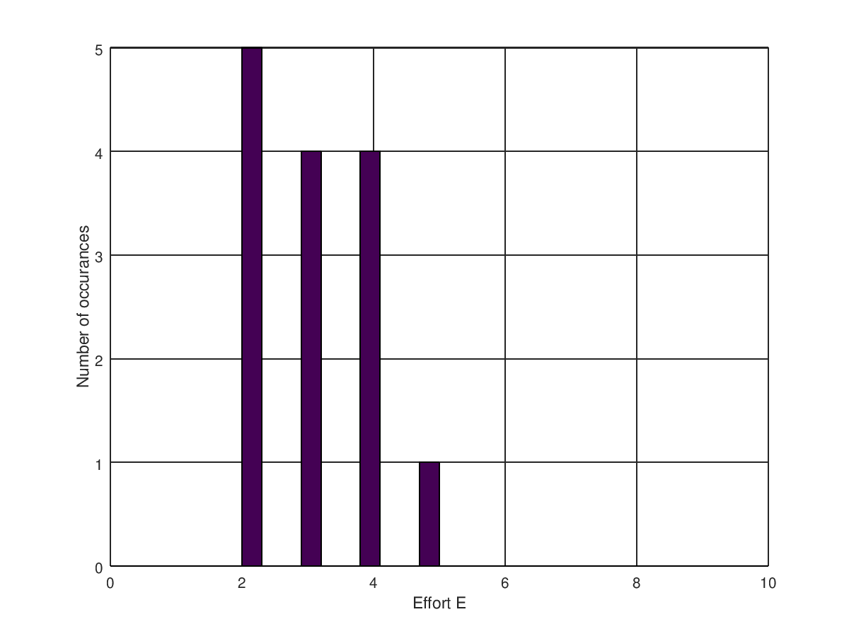
Figure 1: Histogram of the effort involved in production of the word Naturalization.

The entire process of decomposition for the English word Naturalization is shown in Table 8. Note that ˚; ̵9ffiT&TbÆMØT˚ in the VS symbolic form of the word Naturalization and each VS symbol can be represented as a $10$ dimensional vector using the VS basis.

Table 8: VS basis representations of the word Naturalization. Note that ${{{E_{word}}}}=43$ is the difficulty level of the word.

	O	R	$\circ$	$\wedge$	2	Δ	!	$\alpha$	$|$	i	$E$
Rest	[0	0	0	0	0	0	0	0	0	0]	–
˚	[1	0	0	0	0	1	0	0	0	1]	3
;	[1	0	0	1	0	0	0	0	0	0]	3
̵	[1	0	0	0	0	1	0	1	0	0]	3
9	[0	1	1	0	0	0	0	0	0	0]	5
ffi	[1	0	0	0	0	1	0	0	0	0]	4
T	[1	0	1	0	0	0	0	0	0	0]	2
&	[1	0	0	0	0	0	1	0	0	0]	2
T	[1	0	1	0	0	0	0	0	0	0]	2
b	[1	0	0	0	0	1	0	0	0	0]	2
Æ	[0	0	0	0	0	1	0	1	0	0]	2
M	[1	0	0	1	0	0	0	0	0	0]	4
Ø	[0	0	0	0	0	1	0	1	0	0]	4
T	[1	0	1	0	0	0	0	0	0	0]	4
˚	[1	0	0	0	0	1	0	0	0	1]	3
											${{{E_{word}}}}=43$

We now compute the effort ($E$) in terms of moving the organs of speech production system when transitioning from one sound represented in the VS basis as $\vec{R_{i}}$ to the next sound represented in the VS basis as ($\vec{R_{k}}$) as

$$E=\#({\vec{R_{i}}\oplus\vec{R_{k}}})$$

where, $\oplus$ represents the XOR operation and $\#(\vec{R})$ represents the number of $1$’s in the vector $\vec{R}$. The last column in Table 8 shows the effort, $E$, in traversing from one sound to another. For example, $E=3$ for traversing from sound ˚ represented by $R_{\mbox{\vis\char 23\relax}}$ =[ 1, 0, 0, 0, 0, 1, 0, 0, 0, 1] to the sound ; represented by $R_{\mbox{\vis\char 59\relax}}$ = [1, 0, 0, 1, 0, 0, 0, 0, 0, 0] (see Table 8). Note that $\vec{R_{\mbox{\vis\char 23\relax}}}\oplus\vec{R_{\mbox{\vis\char 59\relax}}}$ $=[0,0,0,1,0,1,0,0,0,1$] and $\#([0,0,0,1,0,1,0,0,0,1])=3$. The effort for pronouncing the word Naturalization is the sum of effort taken to traverse from one sound to another while speaking the word. As seen in Table 8 the effort to speak naturalization is ${{{E_{word}}}}=43$.

Figure 1 shows the histogram plot for the effort involved in producing the word Naturalization. Observe that there are $5$ instances when an effort or $E=2$ was required to move from one sound to another. Since, the ability to precisely control the different organs involved in speech production is diminished in dysarthric patients, words that require higher value of effort are usually not articulated properly by these patients. Subsequently words with higher ${{{E_{word}}}}$ are more difficult to articulate because they need speech producing organs to transition more than a simple word.

The effort required to speak a word or equivalently the difficulty level of a word depends on the amount of changes the articulators have to make to articulate that word. We use this in building a cost function (9) to identify an optimal set of words that can be used to assess the intelligibility of spoken speech.

5 Experimental Results

We conducted a series of experiments with an objective to determine how close the proposed intelligibility assessment techniques were to the SLP relatable perceptual intelligibility score. Additionally the aim was to assess the intelligibility score by asking the dysarthric patient speak a very limited number of carefully chosen words. We first detail the database that was used for experimentally validating the proposed speech intelligibility techniques.

5.1 Database

The Dysarthric Speech Database for Universal Access Research (UA Speech database) [63] consists of audiovisual recordings produced by $15$ dysarthric speakers with cerebral palsy and $13$ healthy subjects. The subjects were required to read a set of $765$ isolated words ($449$ unique) shown on a computer monitor. The set of utterances, from each participant, included

• Digits (D) ($10$ words, $3$ repetitions). Example one, two , $\cdots$

• Letters (L) ($26$ words, $3$ repetitions). The $26$ letters of the International Radio Alphabet. Example alpha, bravo, $\cdots$

• Computer Commands (CC) ($19$ words, $3$ repetitions). A set of common word processing commands. Example command, line, enter, $\cdots$

• Common Words (CW) ($100$ words, $3$ repetitions). The most common $100$ words taken from the Brown corpus. Example yes, no, $\cdots$

• Uncommon Words  (UW) ($300$ words, $1$ repetition). Words selected from Project Gutenberg novels such that the occurrence of infrequent biphones is maximized. Example butterflies, convulsion, $\cdots$

As can be observed there should be $455$ ($10$ Digits, $26$ Letters, $19$ Computer Commands, $100$ Common Words, and $300$ Uncommon Words) unique words. However $6$ words (choking, equilibrium, moustache, powwow, vouchsafe, and watch) in Uncommon Words repeat reducing the number of unique words to $449$.

Table 9: Distribution of speaking task into blocks B1, B2 and B3. The number of utterances is shown in $\{\}$ and the repetition number is shown $()$ [11].

	Full $\{765\}$	B1 $\{255\}$	B2 $\{255\}$	B3 $\{255\}$
Computer Commands	CC $\{57\}$	CC(1) $\{19\}$	CC(2) $\{19\}$	CC(3) $\{19\}$
Letters	L $\{78\}$	L(1) $\{26\}$	L(2) $\{26\}$	L(3) $\{26\}$
Digits	D $\{30\}$	D(1) $\{10\}$	D(2) $\{10\}$	D(3) $\{10\}$
Common Words	CW $\{300\}$	CW(1) $\{100\}$	CW(2) $\{100\}$	CW(3) $\{100\}$
Uncommon Words	UW $\{300\}$	UW1 $\{100\}$	UW2 $\{100\}$	UW3 $\{100\}$

All utterances, as mentioned in [63], were recorded using an eight-microphone array at a sampling frequency of $48$ kHz. For ease of subjects, the words were divided into three equally sized blocks (B1, B2, B3) of $255$ words each and the participants were given a break between the blocks. The distribution of utterances in the three blocks is shown in Table 9 for each speaker [11].

A set of $5$ native American English were asked to provide orthographic transcriptions for utterances spoken by dysarthric patients in order to assign a perceptual intelligibility rating. For each listener’s transcription, the percentage of correctly identified transcription was calculated and averaged to obtain the individual speaker’s intelligibility rating based on perception. These intelligibility scores lie in the range of $2\%$ to $95\%$. Further, based on these scores, each speaker was classified into one of four categories: very low $(0\%-25\%)$, low $(26\%-50\%)$, medium $(51\%-75\%)$ and high $(76\%-100\%)$ intelligibility.

5.2 Results

As an attempt to concurrently seize the effects of the proposed techniques, we evaluate the performance of the methods, namely, (i) $I_{os}$ (1), (ii) DeepSpeech + $I_{sm}$ (3), (iii) DeepSpeech + $I_{ld}$ (4) and (iv) DeepSpeech + $I_{<{\tt unk}>}$ (5) on different subsets of utterances from the UASpeech dataset. As mentioned earlier $I_{os}$ is negatively correlated to perceptual intelligibility scores while the other intelligibility scores are positively correlated. The subsets used for our analysis, as seen in Table 9, are (a) Computer Commands (CC), (b) International Radio Letters (Letters), (c) Digits, (d) Common Words  (CW) and (d) Uncommon Words UW1, UW2 and UW3 and across three different blocks, namely, B1, B2 and B3 as shown in Table 10. We also compute the combined average score across all $765$ words using our intelligibility metrics $I_{os}$, DeepSpeech + $I_{sm}$, DeepSpeech + $I_{ld}$, and DeepSpeech + $I_{<{\tt unk}>}$ compared to the perceptual intelligibility (considered as the ground truth) rating using Pc. Since all but Uncommon Words are present in each of the three blocks B1, B2 and B3, the Pc values averaged across the three blocks are of the same range. The low value of Pc for the subset of Digits is attributed to the comparative simplicity in production of the words and hence less effort to pronounce them as described by the visible speech analysis. As we will see later, none of the words in Digits qualify into the optimal set of words that are sufficient to compute the intelligibility score of dysarthric speech. In general the Uncommon Words  are difficult to pronounce and hence the higher value of Pc signifies that the UW subset seems to captures the nuances required for reliable intelligibility estimation. It can also be seen that intelligibility score based on Sequence Matching and Levenshtein distance performs better compared to the other intelligibility measuring metrics.

Table 10: Pearson Correlation of the proposed techniques for assessment of intelligibility.

	CC	Digits	Letters	CW	UW1	UW2	UW3	B1	B2	B3	All Words
Utt/speaker	57	30	78	300	100	100	100	255	255	255	765
$I_{os}$ (1)	-0.80	-0.74	-0.83	-0.81	-0.80	-0.73	-0.74	-0.84	-0.80	-0.73	-0.81
DeepSpeech + $I_{sm}$ (3)	0.85	0.84	0.93	0.94	0.94	0.92	0.92	0.94	0.93	0.94	0.94
DeepSpeech + $I_{ld}$ (4)	0.88	0.84	0.94	0.93	0.91	0.90	0.90	0.93	0.91	0.93	0.93
DeepSpeech + $I_{<{\tt unk}>}$(5)	0.87	0.83	0.88	0.82	0.91	0.90	0.90	0.89	0.88	0.87	0.88

As we argued earlier that it is physically taxing on a patient to speak a large number of utterances, for example, the best performance of intelligibility assessment would require the patient to speak all the $765$ utterances (last column of Table 10). We applied the cost minimization approach, described in Section 4, to identify an optimal (much smaller than $449$) set of words, which would not adversely affect the computation of intelligibility score of the speaker.

Given a set of $|W|$ words, the proposed algorithm requires to look in for $(2^{|W|}-1)$ possible combinations to find the optimal subset $\SS_{k}$ containing $|W_{k}|$ words. In the UASpeech dataset a set of $|W|={{449}}$ unique words are provided which leads to ${\cal T}\approx 10^{{{135}}}$ possible subsets. Note that operating on such high number of possible solutions is infeasible. We used the following two criteria to reduce the number of words from which we expect our word selection to happen

1. All words with less than ${{5}}$ syllables are discarded.

2. For each isolated word, the distance traversed in the 2D vowel space (formed by formants $F_{1}$ and $F_{2}$) is determined using the standard values of formants for vowels shown in Table 11 [64, 65]. The phonetic transcription of each word is obtained and the Euclidean distance between subsequent vowels present in the word are summed up to obtain the distance that is required to be traversed in the vowel space in order to satisfactorily pronounce the word.

   For example, the word Naturalization has the phonetic transcription (using the ARPABET symbol set consists of $39$ phonemes [66]) [’N’, ’AE’, ’CH’, ’ER’, ’AH’, ’L’, ’IH’, ’Z’, ’EY’, ’SH’, ’AH’, ’N’], considering only the vowels, we get [’AE’, ’ER’, ’AH’, ’IH’, ’EY’, ’AH’]. Assuming an initial rest start, namely, $F_{1}=0$ and $F_{2}=0$, for the word the distance traversed in the $F_{1}-F_{2}$ space is calculated as the Euclidean distance between the vowels, namely, ’AE’ (588, 1952) $\rightarrow$ ’ER’ (474, 1379) $\rightarrow$ ’AH’ (623, 1200) $\rightarrow$ ’IH’ (427, 2034) $\rightarrow$ ’EY’ (580, 1799) $\rightarrow$ ’AH’ (623, 1200) is $4593.44$. All words that traversed less than $2400$ in this $F_{1}-F_{2}$ space were discarded.

Table 11: Formant frequencies of F1 and F2 for American English vowels from [65].

Vowel	EY	AO	ER	AH	UW	AE	IY	IH	UH	AA	E
F1	580	652	474	623	378	588	342	427	469	768	476
F2	1799	997	1379	1200	997	1952	2322	2034	1122	1333	2089

The aforementioned constraints reduces the space of words from $449$ to $14$. The set of $14$ words, all from Uncommon Words set are shown in Table 12. We applied the proposed cost minimization approach on this set of $14$ words only. Note that we now have to search for an optimal set of words from ${\cal T}=16384$ possible subsets (see (10)). The performance, in terms of Pc, of the proposed techniques for assessment of intelligibility on these set of $14$ words is also shown in Table 12. Note that this is our reference performance of the four intelligibility techniques. We now apply our cost minimization approach to find the optimal set of words from this set of $14$ words (Table 12).

Table 12: Performance on the set of $14$ words identified from the set of $449$ words, which had more than $5$ syllables and traversed $>2400$ in the $F_{1}$-$F_{2}$ space.

Method	$|W_{k}|$	Pc	Naturalization, Autobiography, Exactitude, Irresolute, Inalienable, Legislature, Overshadowed, Psychological, Dissatisfaction, Agricultural, Apothecary, Authoritative, Exaggerate, Inexhaustible
$I_{os}$	14	-0.81
DeepSpeech + $I_{<{\tt unk}>}$	14	0.91
DeepSpeech + $I_{sm}$	14	0.92
DeepSpeech + $I_{ld}$	14	0.87

In the experiments to follow, we minimize the cost function (9) for different values of $\alpha$’s to identify an optimal set of words ($\SS_{k}^{*}$) and show the performance on this set of words for the four different intelligibility assessment metrics, namely, $I_{os}$, DeepSpeech + $I_{sm}$, DeepSpeech + $I_{ld}$, DeepSpeech + $I_{<{\tt unk}>}$.

Experiment 1

$\SS_{1}^{*}=\min_{k=1,2,\cdots,{\cal T}}\left\{\alpha_{1}|\SS_{k}|-\alpha_{3}{{{E_{word}}}}\left(\SS_{k}\right)\right\}$

This is the case when we do not have access to perceptual intelligibility score, or in other words there is no access to a database of utterances. Clearly, this scenario is (a) independent of the intelligibility assessment technique described in Section 3 (see Table 13) and (b) allows for building a speech intelligibility assessment system for any language using just the dictionary of words without the need for an annotated database.

The optimal set of words for $\alpha_{1}=1,\alpha_{2}=0,\alpha_{3}=1$ is shown in Table 13. As can be seen there is not a significant change in the performance of the intelligibility assessment techniques when a set of $8$ words were selected from $14$ words using the cost minimization approach with $\alpha_{1}=1,\alpha_{2}=0,\alpha_{3}=1$ in (9). This suggests that even in the absence of a database we should be in a position to select a set of words that can be used for intelligibility assessment.

Table 13: Performance on selected optimal set of words for $\alpha_{1}=1,\alpha_{2}=0,\alpha_{3}=1$.

Method	$|\SS_{1}^{*}|$	Pc	Selected Words ($\SS_{1}^{*}$)
$I_{os}$	8	-0.82	Naturalization, Authoritative, Autobiography, Psychological, Dissatisfaction, Agricultural, Apothecary, Inexhaustible
DeepSpeech + $I_{<{\tt unk}>}$	8	0.93
DeepSpeech + $I_{sm}$	8	0.91
DeepSpeech + $I_{ld}$	8	0.85

Experiment 2

$\SS_{2}^{*}=\min_{k=1,2,\cdots,{\cal T}}\left\{\alpha_{1}|\SS_{k}|-\alpha_{2}\mbox{{\tt{cor}}}\left(\SS_{k}\right)\right\}$

This condition $\alpha_{1}=1,\alpha_{2}=1,$ and $\alpha_{3}=0$ does not make use of the component that captures the articulatory effort (based on visual speech) required to utter a word. The optimal set of words for $\alpha_{1}=1,\alpha_{2}=1,\alpha_{3}=0$ is shown in Table 14. Clearly the introduction of effort required to utter a word (computed using visual speech) is a very important factor in the construction of the cost function. As can be seen, the absence of visual speech based effort to utter a word in the cost function (9) results in the selection of only one word. The selected optimal word happens to be the one with the largest Pc depending on the technique used for assessment.

Table 14: Performance on selected optimal set of words for $\alpha_{1}=1,\alpha_{2}=1,\alpha_{3}=0$.

Method	$|\SS_{2}^{*}|$	Pc	Selected Words ($\SS_{2}^{*}$)
$I_{os}$	1	-0.79	Dissatisfaction
DeepSpeech + $I_{<{\tt unk}>}$	1	0.89	Authoritative
DeepSpeech + $I_{sm}$	1	0.88	Naturalization
DeepSpeech + $I_{ld}$	1	0.85	Naturalization

Experiment 3

$\SS_{3}^{*}=\min_{k=1,2,\cdots,{\cal T}}\left\{\alpha_{1}|\SS_{k}|-\alpha_{2}\mbox{{\tt{cor}}}\left(\SS_{k}\right)-\alpha_{3}{{{E_{word}}}}\left(\SS_{k}\right)\right\}$

The optimal value of the number of words ($|\SS_{3}^{*}|$), and the subset of words $\SS_{3}^{*}$ for the four different intelligibility assessment techniques is shown in Table 15. Also shown is the Pc upon performing the intelligibility assessment with the identified optimal set of words. It can be observed that the optimal number of words selected are between $6$ (for $I_{os}$) and $9$ (for DeepSpeech + $I_{sm}$). This is a significant reduction in the number of utterances compared to the $765$ utterances that a dysarthric patient has to speak to enable gauge the intelligibility score ([67, 42, 68]). The automatic identification of an optimal number of words, using a cost minimization approach, for intelligibility assessment is one of the main contributions of this paper. It can be observed that the selected words, in the optimal set, require complex movements and precise control over the organs of the speech production system and hence, are suitable for the purpose of intelligibility assessment.

Table 15: Performance of the proposed techniques after selecting an optimal set words (9) for $\alpha_{1}=\alpha_{2}=\alpha_{3}=1$.

Method	$|\SS_{3}^{*}|$	Pc	Selected Words ($\SS_{3}^{*}$)
$I_{os}$	$6$	$-0.86$	Autobiography, Overshadowed, Psychological, Dissatisfaction, Agricultural, Inexhaustible
DeepSpeech + $I_{<{\tt unk}>}$	$7$	$0.94$	Naturalization, Psychological, Dissatisfaction, Agricultural, Apothecary, Authoritative, Inexhaustible
DeepSpeech + $I_{sm}$	$9$	$0.94$	Naturalization, Authoritative, Exactitude, Overshadowed, Psychological, Dissatisfaction, Agricultural, Apothecary, Inexhaustible,
DeepSpeech + $I_{ld}$	$6$	$0.91$	Inexhaustible, Authoritative, Apothecary, Agricultural, Dissatisfaction, Naturalization

Figure 2 shows a scatter plot of the estimated intelligibility rating based on each of the four proposed approaches, namely, $I_{os}$ (top left), DeepSpeech + $I_{<{\tt unk}>}$ (top right), DeepSpeech + $I_{sm}$ (bottom left) and DeepSpeech + $I_{ld}$ (bottom right) with the perceptual intelligibility rating ($I_{p}$). It can be inferred that the predicted and perceptual assessment scores follow a linear relation throughout the intelligibility range ($0$-$100$). Thus, we establish that even a smaller set of optimally chosen words is indeed sufficient to reliably assess the intelligibility rating of a dysarthric speaker. It can be observed that the Pc of all the proposed techniques (Table 15) based on a set of only $6$ to $9$ spoken words is not very far from the last column of Table 10 which is based on considering all the $765$ utterances spoken by the patient.

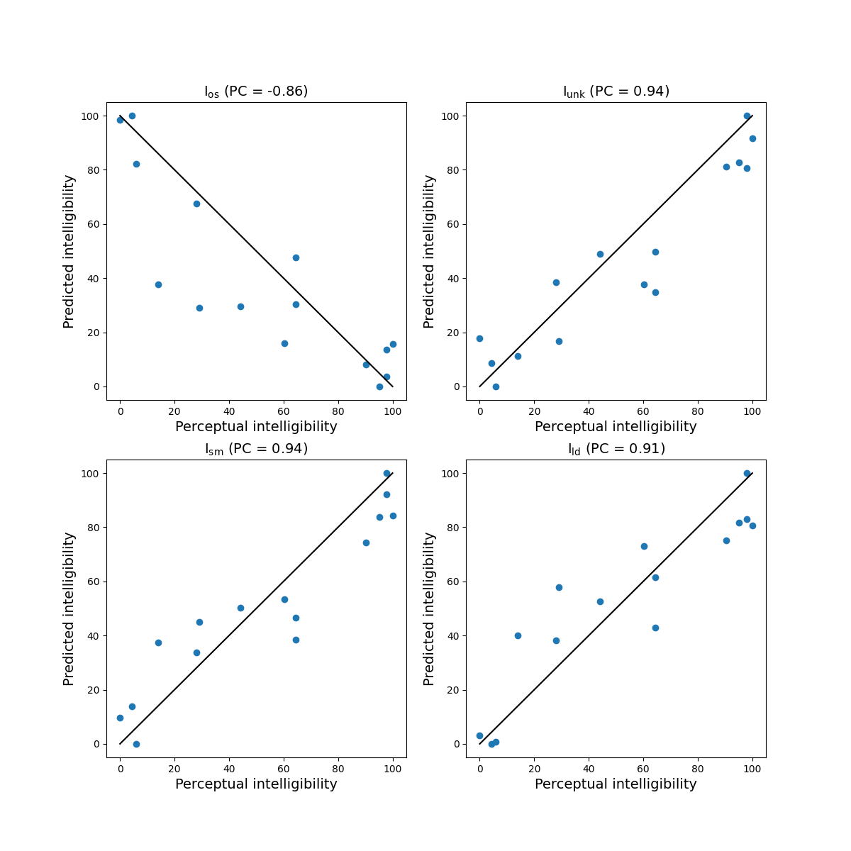
Figure 2: Scatter plot between the perceptual intelligibility ($I_{p}$) and $I_{os}$ (top left), DeepSpeech + $I_{<{\tt unk}>}$ (top right), DeepSpeech + $I_{sm}$ (bottom left) and DeepSpeech + $I_{ld}$ (bottom right).

We further evaluate the proposed four different intelligibility assessment systems with other state-of-the-art techniques in Table 16. In [42], the authors obtained a Pc of $0.91$ using an approach based on a total variability subspace modeled by factor analysis by representing acoustic information corresponding to each speech by an i-vector and then trained a support vector regression model for intelligibility score estimation. Janbakhshi et. al. [68] proposed a reference-based approach called P-STOI by using DTW technique to create utterance dependent healthy references and then computing spectral cross-correlation of aligned pathological speech to the healthy reference in order to assess intelligibility, yielding a Pc of $0.95$. A Mahalanobis distance-based discriminant analysis classifier based on a set of acoustic features, resulted in a Pc of $0.96$ as proposed in [67]. As can be observed, all the DeepSpeech based proposed approaches of assessing the intelligibility of dysarthric speech are very close to (in terms of correlating with perceptual intelligibility score) other state of the art approaches proposed in literature in spite of the fact that our approaches require a significantly smaller number of words to be uttered by the patient (compare $6-9$ utterances to $765$ utterances).

Table 16: Performance of the proposed and state-of-the-art measures on the UA Speech corpus.

Method	Pc
Martinez et. al.[42] (2013)	$0.91$
Janbakhshi et. al.[68] (2019)	$0.95$
Paja et. al.[67] (2012)	$0.96$
$I_{os}$ (Proposed)	$-0.86$
DeepSpeech + $I_{<{\tt unk}>}$ (Proposed)	$0.94$
DeepSpeech + $I_{sm}$ (Proposed)	$0.94$
DeepSpeech + $I_{ld}$ (Proposed)	$0.91$

It can be observed that the word Naturalization appears frequently as one of the words in the optimal set of words selected by minimizing the cost function (9) for varying values of $\alpha$’s (see Tables 13, 14, 15). The performance of the proposed techniques using the single word Naturalization in terms of Pc is captured in Table 17. The main reason for its frequent occurrence can be attributed the fact that it has one of the highest articulatory effort cost (computed based on visual speech) among all the $14$ words (see Table 8) that were used in our experiments to select the optimal set of words.

Table 17: Performance of the proposed techniques on the frequently occurring word Naturalization.

Method	Pc
$I_{os}$	$-0.55$
DeepSpeech + $I_{<{\tt unk}>}$	$0.85$
DeepSpeech + $I_{sm}$	$0.88$
DeepSpeech + $I_{ld}$	$0.93$

6 Conclusion

Dysarthria is a neuro motor disorder that affects the ability of the person to have precise control over his organs that help in producing speech. Determining the intelligibility of speech which is relatable with the perceptual intelligibility score that the SLP is familiar with is important. In this paper, we introduced four different techniques, all speaker independent, that can assist in computing the intelligibility score of a dysarthric speaker. The techniques make use of the output of an end to end pre-trained DeepSpeech speech to alphabet (S2A) engine, which in our opinion is novel. As mentioned earlier, we exploit the fact that lack of intelligibility detoriates the performance of the S2A engine primarily because it has been trained on healthy normal speech. Keeping in mind, the immense stress and difficulty faced by a dysarthric patient to speak a large number of words, we proposed a cost minimization scheme which allows for identification of an optimal set of words that are sufficient to retain the fidelity of speech intelligibility assessment. This formulation of the cost minimization approach to identify the optimal set of words, the use of visual speech to determine the pronunciation difficulty of a word, in our opinion, has never been explored before. Infact the cost minimization approach, as formulated in this paper, can be employed to identify an optimal set of words suitable for intelligibility assessment, given a set of dictionary words in any other language (see Table 13). Experimental results show that the choice of optimal number of words is able to predict the intelligibility score of a dysarthric patient and is linearly proportional to the perceptual intelligibility score, thereby making the proposed system built on optimal set of words usable by a speech language pathologist.

References

- [1] K. G. Shipley, J. G. McAfee, Assessment in speech-language pathology : a resource manual, 4th Edition, Delmar Cengage Learning, 2009.
- [2] M. Edwards, Disorders of Articulation: Aspects of Dysarthria and Verbal Dyspraxia, 1st Edition, Disorders of Human Communication 7, Springer-Verlag Wien, 1984.
- [3] K. M. Yorkston, D. R. Beukelman, Assessment of intelligibility of dysarthric speech, C. C. Publications Inc., 1981.
- [4] P. M. Enderby, Frenchay dysarthria assessment, British Journal of Disorders of Communication 17 (1983) 165–173.
- [5] D. Tanner, W. Culbertson, Quick assessment for dysarthria, Academic Communication Associates, Oceanside, CA, 1999.
- [6] M. Hoehn, M. Yahr, Parkinsonism: onset, progression and mortality, Neurology 17 (1967) 427–442.
- [7] S. Fahn, R. L. Elton, Unified parkinsons disease rating scale, Recent Developments in Parkinsons Disease,Macmillan Health Care Information 2 (1987) 153–163.
- [8] T. Schmitz-Hubsch, Scale for the assessment and rating of ataxia : development of a new clinical scale, Neurology 669 (2006) 1717–1720.
- [9] R. Kent, Some limits to the auditory-perceptual assessment of speech and voice disorders, American Journal of Speech Language Pathology 5 (1996) 7–23.
-
[10]
Viartis, Unified parkinson’s
disease rating scale (Accessed Nov 2020).
URL viartis.net/parkinsons.disease/UPDRS1.pdf - [11] A. Tripathi, S. Bhosale, S. K. Kopparapu, A novel approach for intelligibility assessment in dysarthric subjects, in: ICASSP 2020 - 2020 IEEE International Conference on Acoustics, Speech and Signal Processing (ICASSP), 2020, pp. 6779–6783.
- [12] A. Tripathi, S. Bhosale, S. K. Kopparapu, Improved speaker independent dysarthria intelligibility classification using deepspeech posteriors, in: ICASSP 2020 - 2020 IEEE International Conference on Acoustics, Speech and Signal Processing (ICASSP), 2020, pp. 6114–6118.
- [13] A. Tripathi, S. Bhosale, S. K. Kopparapu, Automatic speech intelligibility assessment in dysarthric subjects, in: Fourteenth International Conference on Digital Society, ICDS, 2020, pp. 1–4.
- [14] J. R. O. Arroyave, J. F. V. Bonilla, E. D. Trejos, Acoustic analysis and non linear dynamics applied to voice pathology detection: A review, Recent Patents on Signal Processing 2.
- [15] J. Mekyska, E. Janousova, P. Gomez-Vilda, Z. Smekal, I. Rektorova, I. Eliasova, M. Kostalova, M. Mrackova, J. B. Alonso-Hernandez, M. Faundez-Zanuy, K. L. de Ipiña, Robust and complex approach of pathological speech signal analysis, Neurocomputing 167 (2015) 94 – 111.
-
[16]
S. Hegde, S. Shetty, S. Rai, T. Dodderi,
A
survey on machine learning approaches for automatic detection of voice
disorders, Journal of Voice 33 (6) (2019) 947.e11–947.e33.
doi:https://doi.org/10.1016/j.jvoice.2018.07.014.
URL https://www.sciencedirect.com/science/article/pii/S0892199718301437 - [17] C. Bhat, B. Vachhani, S. K. Kopparapu, Automatic assessment of dysarthria severity level using audio descriptors, in: 2017 IEEE International Conference on Acoustics, Speech and Signal Processing (ICASSP), 2017, pp. 5070–5074.
- [18] S. K. Kopparapu, Non-Linguistic Analysis of Call Center Conversations, 1st Edition, SpringerBriefs in Electrical and Computer Engineering, Springer International Publishing, 2015.
- [19] J. Kim, N. Kumar, A. Tsiartas, M. Li, S. S. Narayanan, Automatic intelligibility classification of sentence-level pathological speech, Computer speech & language 29 (1) (2015) 132–144.
- [20] F. Rudzicz, Articulatory knowledge in the recognition of dysarthric speech, IEEE Transactions on Audio, Speech, and Language Processing 19 (4) (2010) 947–960.
- [21] M. Vasilakis, Y. Stylianou, Voice pathology detection based on short-term jitter estimations in running speech, Folia Phoniatr Logop 61 (2009) 153–170.
- [22] S. Skodda, W. Visser, U. Schlegel, Short- and long-term dopaminergic effects on dysarthria in early parkinson’s disease, J Neural Transm 117 (2010) 197–205.
- [23] M. A. Little ∗, P. E. McSharry, E. J. Hunter, J. Spielman, L. O. Ramig, Suitability of dysphonia measurements for telemonitoring of parkinson’s disease, IEEE Transactions on Biomedical Engineering 56 (4) (2009) 1015–1022.
-
[24]
J. Shao, J. K. MacCallum, Y. Zhang, A. Sprecher, J. J. Jiang,
Acoustic
analysis of the tremulous voice: Assessing the utility of the correlation
dimension and perturbation parameters, Journal of Communication Disorders
43 (1) (2010) 35 – 44.
URL http://www.sciencedirect.com/science/article/pii/S0021992409000690 - [25] D. Dimitriadis, A. Potamianos, P. Maragos, A comparison of the squared energy and teager-kaiser operators for short-term energy estimation in additive noise, IEEE Transactions on Signal Processing 57 (7) (2009) 2569–2581.
- [26] M. González-Izal, I. Rodríguez-Carreño, A. Malanda, F. Mallor-Giménez, I. Navarro-Amézqueta, E. Gorostiaga, M. Izquierdo, sEMG wavelet-based indices predicts muscle power loss during dynamic contractions, Journal of Electromyography and Kinesiology 20 (6) (2010) 1097 – 1106.
- [27] Yu Song, Wen-Hong Wang, Feng-Juan Guo, Feature extraction and classification for audio information in news video, in: 2009 International Conference on Wavelet Analysis and Pattern Recognition, 2009, pp. 43–46.
- [28] K. M. Allison, L. Annear, M. Policicchio, K. C. Hustad, Range and precision of formant movement in pediatric dysarthria., Journal of speech, language, and hearing research : JSLHR 60 7 (2017) 1864–1876.
- [29] K. L. Lansford, J. M. Liss, Vowel acoustics in dysarthria: speech disorder diagnosis and classification., Journal of speech, language, and hearing research : JSLHR 57 1 (2014) 57–67.
- [30] A. K. Dubey, A. Tripathi, S. R. M. Prasanna, S. Dandapat, Detection of hypernasality based on vowel space area, The Journal of the Acoustical Society of America 143 (5) (2018) EL412–EL417.
- [31] N. P. Narendra, P. Alku, Glottal source information for pathological voice detection, IEEE Access 8 (2020) 67745–67755.
- [32] K. Gurugubelli, A. K. Vuppala, Analytic phase features for dysarthric speech detection and intelligibility assessment, Speech Communication 121 (2020) 1 – 15.
- [33] C. Bhat, B. Vachhani, S. K. Kopparapu, Automatic assessment of dysarthria severity level using audio descriptors, in: 2017 IEEE International Conference on Acoustics, Speech and Signal Processing (ICASSP), 2017, pp. 5070–5074.
- [34] D. Korzekwa, R. Barra-Chicote, B. Kostek, T. Drugman, M. Lajszczak, Interpretable Deep Learning Model for the Detection and Reconstruction of Dysarthric Speech, in: Proc. Interspeech 2019, 2019, pp. 3890–3894.
- [35] M. Perez, W. Jin, D. Le, N. Carlozzi, P. Dayalu, A. Roberts, E. M. Provost, Classification of huntington disease using acoustic and lexical features, in: ISCA Interspeech, 2018, pp. 1898–1902.
- [36] J. Mallela, A. Illa, S. B. N, S. Udupa, Y. Belur, N. Atchayaram, R. Yadav, P. Reddy, D. Gope, P. K. Ghosh, Voice based classification of patients with amyotrophic lateral sclerosis, parkinson’s disease and healthy controls with cnn-lstm using transfer learning, in: ICASSP 2020 - 2020 IEEE International Conference on Acoustics, Speech and Signal Processing (ICASSP), 2020, pp. 6784–6788.
- [37] A. Mayle, Z. Mou, R. Bunescu, S. Mirshekarian, L. Xu, C. Liu, Diagnosing Dysarthria with Long Short-Term Memory Networks, in: Proc. Interspeech 2019, 2019, pp. 4514–4518.
- [38] H. M. Chandrashekar, V. Karjigi, N. Sreedevi, Spectro-temporal representation of speech for intelligibility assessment of dysarthria, IEEE Journal of Selected Topics in Signal Processing 14 (2) (2020) 390–399.
- [39] C. Bhat, H. Strik, Automatic assessment of sentence-level dysarthria intelligibility using blstm, IEEE Journal of Selected Topics in Signal Processing 14 (2) (2020) 322–330.
- [40] K. An, M. J. Kim, K. Teplansky, J. R. Green, T. Campbell, Y. Yunusova, D. Heitzman, J. Wang, Automatic early detection of amyotrophic lateral sclerosis from intelligible speech using convolutional neural networks, in: INTERSPEECH, 2018.
- [41] T. Bocklet, K. Riedhammer, E. Nöth, U. Eysholdt, T. Haderlein, Automatic intelligibility assessment of speakers after laryngeal cancer by means of acoustic modeling, Journal of Voice 26 (3) (2012) 390 – 397.
- [42] D. Martinez, P. Green, H. Christensen, Dysarthria intelligibility assessment in a factor analysis total variability space, in: ISCA Interspeech, 2013, pp. 2133–2137.
- [43] D. Martínez, E. Lleida, P. Green, H. Christensen, A. Ortega, A. Miguel, Intelligibility assessment and speech recognizer word accuracy rate prediction for dysarthric speakers in a factor analysis subspace, ACM Trans. Access. Comput. 6 (3).
- [44] I. Laaridh, W. B. Kheder, C. Fredouille, C. Meunier, Automatic prediction of speech evaluation metrics for dysarthric speech, in: Proc. Interspeech 2017, 2017, pp. 1834–1838.
- [45] C. M. Vikram, A. Tripathi, S. Kalita, S. R. M. Prasanna, Estimation of hypernasality scores from cleft lip and palate speech, in: Proc. Interspeech 2018, 2018, pp. 1701–1705.
- [46] M. Saxon, A. Tripathi, Y. Jiao, J. Liss, V. Berisha, Robust estimation of hypernasality in dysarthria with acoustic model likelihood features (2019). arXiv:1911.11360.
- [47] C. Middag, Y. Saeys, J.-P. Martens, Towards an asr-free objective analysis of pathological speech, in: Proc. Interspeech 2010, 2010, pp. 294–297.
- [48] C. Middag, J.-P. Martens, G. Van Nuffelen, M. De Bodt, Automated intelligibility assessment of pathological speech using phonological features, EURASIP J. Adv. Signal Process 2009.
- [49] M. Schuster, E. Noth, T. Haderlein, S. Steidl, A. Batliner, F. Rosanowski, Can you understand him? let’s look at his word accuracy-automatic evaluation of tracheoesophageal speech, in: Proceedings. (ICASSP ’05). IEEE International Conference on Acoustics, Speech, and Signal Processing, 2005., Vol. 1, 2005, pp. I/61–I/64 Vol. 1.
- [50] A. K. Maier, M. Schuster, A. Batliner, E. Nöth, E. Nkenke, Automatic scoring of the intelligibility in patients with cancer of the oral cavity, in: INTERSPEECH, 2007.
- [51] A. Maier, T. Haderlein, F. Stelzle, E. Nöth, E. Nkenke, F. Rosanowski, A. Schützenberger, M. Schuster, Automatic speech recognition systems for the evaluation of voice and speech disorders in head and neck cancer, EURASIP J. Audio Speech Music Process. 2010 (1).
- [52] M. Schuster, T. Haderlein, E. Nöth, J. Lohscheller, U. Eysholdt, F. Rosanowski, Intelligibility of laryngectomees’ substitute speech: automatic speech recognition and subjective rating, European Archives of OtoRhinoLaryngology and Head & Neck 263 (2005) 188–193.
- [53] P. Janbakhshi, I. Kodrasi, H. Bourlard, Synthetic speech references for automatic pathological speech intelligibility assessment, in: ICASSP 2020 - 2020 IEEE International Conference on Acoustics, Speech and Signal Processing (ICASSP), 2020, pp. 6099–6103.
- [54] P. Janbakhshi, I. Kodrasi, H. Bourlard, Spectral Subspace Analysis for Automatic Assessment of Pathological Speech Intelligibility, in: Proc. Interspeech 2019, 2019, pp. 3038–3042.
- [55] opensmile, http://www.audeering.com/research/opensmile.
- [56] S. H. Dumpala, R. Chakraborty, S. K. Kopparapu, Audio-visual fusion for sentiment classification using cross-modal autoencoder, in: Visually Grounded Interaction and Language (ViGIL) NeurIPS 2018 Workshop, Montreal, Canada, 2018.
- [57] C. Bhat, S. K. Kopparapu, Identification of alzheimer’s disease using non-linguistic audio descriptors, in: EUSIPCO 2019, Spain, 2019.
- [58] B. W. Schuller, S. Steidl, A. Batliner, The interspeech 2009 emotion challenge, in: INTERSPEECH, 2009.
- [59] Mozilla, Deepspeech, https://github. com/mozilla/DeepSpeech/releases (Jan 2019).
- [60] V. Panayotov, G. Chen, D. Povey, S. Khudanpur, Librispeech: an asr corpus based on public domain audio books, in: 2015 IEEE International Conference on Acoustics, Speech and Signal Processing (ICASSP), IEEE, 2015, pp. 5206–5210.
- [61] P. E. Black, Ratcliff obershelp pattern recognition, Dictionary of algorithms and data structures, 2004 17.
- [62] A. M. Bell, Visible Speech: The Science of Universal Alphabetics, Simpkin Marshall and Co: London, 1867.
- [63] H. Kim, M. Hasegawa-Johnson, A. Perlman, J. Gunderson, T. Huang, K. Watkin, S. Frame, Dysarthric speech database for universal access research, in: ISCA Interspeech, 2008, pp. 1741–1744.
- [64] S. Scherer, G. M. Lucas, J. Gratch, A. Skip Rizzo, L. Morency, Self-reported symptoms of depression and ptsd are associated with reduced vowel space in screening interviews, IEEE Transactions on Affective Computing 7 (1) (2016) 59–73.
- [65] B. Lindblom, Explaining phonetic variation: A sketch of the h&h theory (1990).
- [66] CMU, Cmu dictionary, http://www.speech.cs.cmu.edu/cgi-bin/cmudict (Accessed Nov 2020).
- [67] M. S. Paja, T. H. Falk, Automated dysarthria severity classification for improved objective intelligibility assessment of spastic dysarthric speechy, in: ISCA Interspeech, 2012, pp. 62–65.
- [68] P. Janbakhshi, I. Kodrasi, H. Bourlard, Pathological speech intelligibility assessment based on the short-time objective intelligibility measure, in: ICASSP 2019 - 2019 IEEE International Conference on Acoustics, Speech and Signal Processing (ICASSP), 2019, pp. 6405–6409.