Vector resonance $X_{1}(2900)$ and its structure

Abstract

The new vector resonance $X_{1}(2900)$ observed recently by LHCb in the $D^{-}K^{+}$ invariant mass distribution in the decay $B^{+}\to D^{+}D^{-}K^{+}$ is studied to uncover internal structure of this state, and calculate its physical parameters. In the present paper, the resonance $X_{1}(2900)$ is modeled as an exotic vector state, $J^{P}=1^{-}$, built of the light diquark $u^{T}C\gamma_{5}d$ and heavy antidiquark $\overline{c}\gamma_{\mu}\gamma_{5}C\overline{s}^{T}$. The mass and current coupling of $X_{1}(2900)$ are computed using the QCD two-point sum rule approach by taking into account various vacuum condensates up to dimension $10$. The width of the resonance $X_{1}(2900)$ is saturated by two decay channels $X_{1}\to D^{-}K^{+}$ and $X_{1}\to\overline{D}^{0}K^{0}$. The strong couplings $g_{1}$ and $g_{2}$ corresponding to the vertices $X_{1}D^{-}K^{+}$ and $X_{1}\overline{D}^{0}K^{0}$ are evaluated in the context of the QCD light-cone sum rule method and technical tools of the soft-meson approximation. Results for the mass of the resonance $X_{1}(2900)$ $m=(2890~{}\pm 122)~{}\mathrm{MeV}$, and for its full width $\Gamma_{\mathrm{full}}=(93\pm 13)~{}\mathrm{MeV}$ are smaller than their experimental values reported by the LHCb collaboration. Nevertheless, by taking into account theoretical and experimental errors of investigations, interpretation of the state $X_{1}(2900)$ as the vector tetraquark does not contradict to the LHCb data. We also point out that analysis of the invariant mass distribution $D^{+}K^{+}$ in the same decay $B^{+}\to D^{+}D^{-}K^{+}$ may reveal doubly charged four-quark structures $[uc][\overline{s}\overline{d}]$.

I Introduction

Recently the LHCb collaboration reported on two new resonant structures $X_{0}(2900)$ and $X_{1}(2900)$ (hereafter $X_{0}$ and $X_{1}$) revealed in the $D^{-}K^{+}$ mass distribution in the process $B^{+}\rightarrow D^{+}D^{-}K^{+}$ LHCb:2020A ; LHCb:2020 . The collaboration measured the masses and widths of these structures, as well as determined their spin-parities. It turned out, that $X_{0}$ and $X_{1}$ are scalar and vector resonances, respectively, and have close masses. These resonance-like peaks are first evidence for exotic mesons composed of four quarks of different flavors provided they can be considered as real resonances. In fact, from decay channels of $X_{0}$ and $X_{1}$, it is clear that they contain four valence quarks $ud\overline{s}\overline{c}$, which put these structures to exclusive place in the $XYZ$ family of exotic mesons.

This discovery triggered interesting theoretical investigations in the context of various models aimed to account for internal organization of the resonances $X_{0}$ and $X_{1}$ and calculate their parameters Karliner:2020vsi ; Wang:2020xyc ; Chen:2020aos ; Liu:2020nil ; Molina:2020hde ; Hu:2020mxp ; He:2020jna ; Liu:2020orv ; Lu:2020qmp ; Zhang:2020oze ; Huang:2020ptc ; Xue:2020vtq ; Yang:2021izl ; Wu:2020job ; Abreu:2020ony ; Wang:2020prk ; Xiao:2020ltm ; Dong:2020rgs ; Burns:2020xne ; Bondar:2020eoa ; Chen:2020eyu ; Albuquerque:2020ugi ; Chen:2021erj . In these articles various assumptions were made about quark-gluon structure of the states $X_{0}$ and $X_{1}$, considered their production mechanisms and decay channels. Investigations were performed in the context of different models by applying numerous methods and calculational schemes. Thus, $X_{0}$ was treated as a scalar tetraquark $X_{0}=[sc][\overline{u}\overline{d}]$ in Refs. Karliner:2020vsi ; Wang:2020xyc , whereas in the papers Chen:2020aos ; Liu:2020nil ; Molina:2020hde ; Hu:2020mxp the $X_{0}$ was interpreted as a scalar molecule $D^{\ast-}K^{\ast+}$. Similar situation emerges in articles devoted to analysis of the vector resonance $X_{1}$. For example, the diquark-antidiquark $X_{1}=[ud][\overline{s}\overline{c}]$ and molecule pictures for $X_{1}$ were proposed in Refs. Chen:2020aos ; He:2020jna , respectively. The structures $X_{0}$ and $X_{1}$, and in general, tetraquarks $\overline{c}\overline{s}qq$ and $sQ\overline{q}\overline{q}$ were investigated in the quark models as well Wang:2020prk ; Yang:2021izl .

Recently, we considered the resonance $X_{0}$ as a bound state of conventional mesons $\overline{D}^{\ast 0}K^{\ast 0}$ Agaev:2020nrc . We calculated its mass and width and found for these parameters $2868\pm 198~{}\mathrm{MeV}$ and $49.6\pm 9.3~{}\mathrm{MeV}$, respectively. These results are in a nice agreement with the LHCb data, which allowed us to classify $X_{0}$ as a hadronic molecule state.

However, two enhancements $X_{0}$ and $X_{1}$ in the $D^{-}K^{+}$ mass distribution may have alternative origin. In fact, the authors of   Ref. Liu:2020orv studied the decay $B^{+}\rightarrow D^{+}D^{-}K^{+}$ via rescattering diagrams $\chi_{c1}D^{\ast-}K^{\ast+}$ and $D_{sJ}\overline{D}_{1}^{0}K^{0}$. It was claimed that, two resonance-like peaks found around thresholds $D^{\ast-}K^{\ast+}$ and $\overline{D}_{1}^{0}K^{0}$ may simulate the states $X_{0}$ and $X_{1}$ without a necessity to introduce genuine four-quark mesons. Appearance of two peaks $X_{0}$ and $X_{1}$ was explained there by the triangle singularities in the scattering amplitudes located in the vicinity of the physical boundary.

This rather brief glance at the literature is enough to see that existing interpretations of $X_{0}$ and $X_{1}$ are controversial and far from being clear. Although among various approaches diquark-antidiquark and hadronic molecule models are dominant ones, alternative assumptions deserve detailed studies as well.

It is worth emphasizing that exotic mesons composed of four quarks of different flavors already attracted interests of scientists, and valuable information was collected on their properties. Investigations of such structures were inspired by observation of the state $X(5568)$, though it was not confirmed later by other experiments. Nevertheless, performed analyses led to considerable theoretical progress in understanding of relevant problems. Indeed, the fully open flavor scalar tetraquark $X_{c}=[su][\overline{c}\overline{d}]$ was considered in Refs. Agaev:2016lkl and Chen:2016mqt . Doubly charged tetraquarks $Z_{\overline{c}s}=[sd][\overline{u}\overline{c}]$ with spin-parities $J^{\mathrm{P}}=0^{+},0^{-}$ and $1^{+}$ were explored in our paper Agaev:2017oay .

The tetraquarks $Z_{\overline{c}s}$ are built of four different quarks as the resonances $X_{0}$ and $X_{1}$, but bear two units of electric charge and are objects of special interest. In Ref. Agaev:2017oay the masses and full widths of these states were computed in the framework of the QCD sum rule method. It is instructive to compare parameters of the axial-vector tetraquark $Z_{\mathrm{AV}}$ with ones of $X_{1}$ although they are states of different structures and parities. In accordance with our result, the mass $m_{\mathrm{AV}}=2826_{-157}^{+134}\ \mathrm{MeV}$ of $Z_{\mathrm{AV}}$ is comparable with the mass of the state $X_{1}$. But $Z_{\mathrm{AV}}$ has the full width $\Gamma_{\mathrm{AV}}=(47.3\pm 11.1)\ \mathrm{MeV}$ and is narrower than the structure $X_{1}$. This is in contrast to the case of scalar and pseudoscalar tetraquarks $X_{c}$, $Z_{\mathrm{S}}$ and $Z_{\mathrm{PS}}$, ground-state masses of which are lower than the mass of $X_{0}$. Such comparison allows us to conclude that the vector tetraquark $[ud][\overline{c}\overline{s}]$ has certain chances to explain observed experimental features of $X_{1}$.

In the present article, we are going to explore the vector resonance $X_{1}$ by assuming that it is a genuine exotic diquark-antidiquark state $X_{1}=[ud][\overline{c}\overline{s}]$. Parameters of $X_{1}$ reported by the LHCb collaboration are:

$$m_{1} = (2904\pm 5\pm 1)~{}\mathrm{MeV},\$$

$$\Gamma_{1} = (110\pm 11\pm 4)~{}\mathrm{MeV}.$$ (1)

We calculate the mass and current coupling of the tetraquark $X_{1}$ by means of the QCD two-point sum rules. Results obtained for these parameters are used to evaluate the partial widths of $P$-wave decays $X_{1}\rightarrow D^{-}K^{+}$ and $X_{1}\rightarrow\overline{D}^{0}K^{0}$ in order to estimate full width of the resonance $X_{1}$. Our predictions will be compared with the LHCb data to check validity of suggestions made about a diquark nature of $X_{1}$.

This paper is organized in the following way: In Section II, we calculate the mass and coupling of the vector tetraquark $[ud][\overline{c}\overline{s}]$. In Section III, we calculate the strong couplings $g_{1}$ and $g_{2}$ corresponding to vertices $X_{1}D^{-}K^{+}$ and $X_{1}\overline{D}^{0}K^{0}$. To this end, we use the QCD light-cone sum rule (LCSR) method and the soft-meson approximation. In this section we find the partial widths of the processes $X_{1}\rightarrow D^{-}K^{+}$ and $X_{1}\rightarrow\overline{D}^{0}K^{0}$.  Here, the full width of $X_{1}$ is evaluated as well. In Section IV, we discuss obtained results, propose to study $D^{+}K^{+}$ invariant mass distribution in decay $B^{+}\rightarrow D^{+}D^{-}K^{+}$ to observe hypothetical yet doubly charged scalar and vector tetraquarks $[uc][\overline{s}\overline{d}]$, and conclude with brief notes.

II The mass and coupling of $X_{1}$

The mass $m$ and current coupling $f$ of the vector tetraquark $[ud][\overline{c}\overline{s}]$ are among key ingredients to check the assumption about diquark-antidiquark nature of the resonance $X_{1}$. First, the mass of $X_{1}$ was measured experimentally, therefore prediction obtained for $m$ should be confronted directly with $m_{1}$. Additionally, the spectroscopic parameters $m$ and $f$  are necessary to find partial widths of the strong decays $X_{1}\rightarrow D^{-}K^{+}$  and $X_{1}\rightarrow\overline{D}^{0}K^{0}$, and evaluate full width of $X_{1}$.

We compute $m$ and $f$ in the context of the QCD two-point sum rule method Shifman:1978bx ; Shifman:1978by . It is one of the effective nonperturbative approaches to determine parameters of the conventional hadrons and explore their different decay channels. But this method can also be applied to study properties of the exotic hadrons. Indeed, the masses and couplings (or residues) of various tetraquarks, their different decay channels were investigated within the QCD sum rule method (see, for example, the review articles Chen:2016qju ; Chen:2016spr ; Albuquerque:2018jkn ; Agaev:2020zad ),

Starting point in our analysis to derive sum rules for $m$ and $f$ is the two-point correlation function

$$\Pi_{\mu\nu}(p)=i\int d^{4}xe^{ipx}\langle 0|\mathcal{T}\{J_{\mu}(x)J_{\nu}^{{\dagger}}(0)\}|0\rangle.$$ (2)

Here, $\mathcal{T}$ stands for the time-ordered product of two currents, and $J_{\mu}(x)$ is the interpolating current for $X_{1}$. The current for the vector diquark-antidiquark state $X_{1}$ can be written down in the following form

$$J_{\mu}(x)=\varepsilon\widetilde{\varepsilon}[u_{b}^{T}(x)C\gamma_{5}d_{c}(x)][\overline{c}_{m}(x)\gamma_{\mu}\gamma_{5}C\overline{s}_{n}^{T}(x)],$$ (3)

where $\varepsilon\widetilde{\varepsilon}=\varepsilon^{abc}\varepsilon^{amn}$, and $a$, $b$, $c$, $m$ and $n$ are color indices. In Eq. (3) $u(x)$, $d(x)$, $c(x)$ and $s(x)$ are the quark fields, whereas $C$ denotes the charge-conjugation operator. The isoscalar current $J_{\mu}(x)$ for the tetraquark $X_{1}$ with quantum numbers $J^{\mathrm{P}}=1^{-}$ is built of the light scalar diquark $uC\gamma_{5}d$ and heavy vector antidiquark $\overline{c}\gamma_{\mu}\gamma_{5}C\overline{s}$, which belongs to antitriplet and triplet representations of the color group, respectively. As a result, the interpolating current $J_{\mu}(x)$ belongs to $[\overline{\mathbf{3}}_{c}]\otimes[\mathbf{3}_{c}]$ representation of $SU_{c}(3)$, and is a colorless construction.

To derive desired sum rules for parameters of $X_{1}$, we have to represent the correlation function $\Pi_{\mu\nu}(p)$ in terms of these parameters, and get the phenomenological side of the sum rules $\Pi_{\mu\nu}^{\mathrm{Phys}}(p)$. In terms of the tetraquark’s parameters the correlation function has the following form

$$\Pi_{\mu\nu}^{\mathrm{Phys}}(p)=\frac{\langle 0|J_{\mu}|X_{1}\rangle\langle X_{1}|J_{\nu}^{\dagger}|0\rangle}{m^{2}-p^{2}}+\cdots.$$ (4)

Expression (4) is obtained by saturating the correlation function $\Pi_{\mu\nu}(p)$ with a complete set of $J^{\mathrm{P}}=1^{-}$ states and performing integration over $x$ in Eq. (2): Contributions of higher resonances and continuum states in $X_{1}$ channel are shown by dots.

The correlator $\Pi_{\mu\nu}^{\mathrm{Phys}}(p)$ can be detailed by introducing the matrix element

$$\langle 0|J_{\mu}|X_{1}\rangle=fm\epsilon_{\mu},$$ (5)

where $\epsilon_{\mu}$ is the polarization vector of the state $X_{1}$. Then $\Pi_{\mu\nu}^{\mathrm{Phys}}(p)$ takes the following form

$$\Pi_{\mu\nu}^{\mathrm{Phys}}(p)=\frac{m^{2}f^{2}}{m^{2}-p^{2}}\left(-g_{\mu\nu}+\frac{p_{\mu}p_{\nu}}{m^{2}}\right)+\cdots,$$ (6)

and contains in parentheses the Lorentz structure of the vector state. A part of this structure proportional to $g_{\mu\nu}$ receives contribution only from vector states, therefore in our analysis we use this term and corresponding invariant amplitude $\Pi^{\mathrm{Phys}}(p^{2})$.

We approximate the phenomenological side of the sum rule $\Pi_{\mu\nu}^{\mathrm{Phys}}(p)$ in Eq. (4) using a simple-pole term. For multiquark hadrons such treatment may give rise to some doubts, because $\Pi_{\mu\nu}^{\mathrm{Phys}}(p)$ contains also contributions of two-hadron reducible terms. Indeed, the relevant interpolating current interacts not only to a multiquark hadron, but couples also with two conventional hadrons lying below the mass of the multiquark system Kondo:2004cr ; Lee:2004xk . Such two-hadron states generate the finite width $\Gamma(p)$ of the multiquark hadron, and modify the quark propagator

$$\frac{1}{m^{2}-p^{2}}\rightarrow\frac{1}{m^{2}-p^{2}-i\sqrt{p^{2}}\Gamma(p)}.$$ (7)

In the case of the tetraquark, these effects rescale its coupling $f$ leaving fixed the mass $m$. Detailed analyses demonstrated that two-hadron contributions as a whole, and two-meson ones in particular are small, and can be neglected Lee:2004xk ; Wang:2015nwa ; Agaev:2018vag ; Sundu:2018nxt . Therefore, in Eq. (4) we use the zero-width single-pole approximation.

The QCD side of the sum rules $\Pi_{\mu\nu}^{\mathrm{OPE}}(p)$ should be computed in the operator product expansion ($\mathrm{OPE}$) with some accuracy. To get $\Pi_{\mu\nu}^{\mathrm{OPE}}(p)$, we insert into Eq. (2) the interpolating current $J(x)$, and contract relevant heavy and light quark fields. After these operations, for $\Pi^{\mathrm{OPE}}(p)$ we find

$$\Pi_{\mu\nu}^{\mathrm{OPE}}(p)=i\int d^{4}xe^{ipx}\varepsilon\widetilde{\varepsilon}\varepsilon^{\prime}\widetilde{\varepsilon}^{\prime}\mathrm{Tr}\left[\gamma_{5}\widetilde{S}_{u}^{bb^{\prime}}(x)\gamma_{5}S_{d}^{cc^{\prime}}(x)\right]$$

$$\times\mathrm{Tr}\left[\gamma_{\mu}\gamma_{5}\widetilde{S}_{s}^{n^{\prime}n}(-x)\gamma_{5}\gamma_{\nu}S_{c}^{m^{\prime}m}(-x)\right],$$ (8)

where $\widetilde{S}_{c(q)}(x)=CS^{T}_{c(q)}C$. Here, $S_{c}(x)$ and $S_{u(s,d)}(x)$ are the heavy $c$- and light $u(s,d)$-quark propagators, respectively. Their explicit expressions are presented, for example, in Ref. Agaev:2020zad . We denote by $\Pi^{\mathrm{OPE}}(p^{2})$ the invariant amplitude corresponding to the structure $g_{\mu\nu}$ in Eq. (8), and use it in our following investigations.

The sum rules for the parameters $m$ and $f$ can be found by equating $\Pi^{\mathrm{Phys}}(p^{2})$ and $\Pi^{\mathrm{OPE}}(p^{2})$ and carrying out usual operations necessary in QCD sum rule computations. These operations include the Borel transformation of the invariant amplitudes and subtraction higher resonances and continuum terms from the phenomenological side using the assumption on the quark-hadron duality. After these manipulations, the sum rules acquire dependence on the Borel $M^{2}$ and continuum threshold $s_{0}$ parameters.

The sum rules for $m$ and $f$ read

$$m^{2}=\frac{\Pi^{\prime}(M^{2},s_{0})}{\Pi(M^{2},s_{0})},$$ (9)

and

$$f^{2}=\frac{e^{m^{2}/M^{2}}}{m^{2}}\Pi(M^{2},s_{0}).$$ (10)

Here, $\Pi(M^{2},s_{0})$ is the Borel transformed and subtracted invariant amplitude $\Pi^{\mathrm{OPE}}(p^{2})$, and $\Pi^{\prime}(M^{2},s_{0})=d/d(-1/M^{2})\Pi(M^{2},s_{0})$.

The function $\Pi(M^{2},s_{0})$ has the following form

$$\Pi(M^{2},s_{0})=\int_{\mathcal{M}^{2}}^{s_{0}}ds\rho^{\mathrm{OPE}}(s)e^{-s/M^{2}}+\Pi(M^{2}).$$ (11)

In this paper we neglect the mass of the $u$ and $d$ quarks, therefore in Eq. (11) $\mathcal{M}=m_{c}+m_{s}$. The spectral density $\rho^{\mathrm{OPE}}(s)$ is found as an imaginary part of the correlation function and encompasses essential piece of $\Pi^{\mathrm{OPE}}_{\mu\nu}(p)$. The Borel transformations of remaining terms in $\Pi^{\mathrm{OPE}}_{\mu\nu}(p)$ are included into $\Pi(M^{2})$: the latter was calculated directly from the expression of $\Pi^{\mathrm{OPE}}_{\mu\nu}(p)$.

Computations are performed by including into analysis vacuum condensates up to dimension $10$. We use the basic quark, gluon and mixed condensates, as well as higher ones obtained as their products: We assume that the factorization of higher dimensional contributions does not generate large ambiguities. We do not provide here analytical expressions of $\rho^{\mathrm{OPE}}(s)$ and $\Pi(M^{2})$, because they are rather lengthy.

The numerical values of the basic condensates were extracted from analysis of different hadronic processes, and are well known parameters Shifman:1978bx ; Shifman:1978by ; Ioffe:2005ym

$$\langle\overline{q}q\rangle=-(0.24\pm 0.01)^{3}~{}\mathrm{GeV}^{3},\ \langle\overline{s}s\rangle=(0.8\pm 0.1)\langle\overline{q}q\rangle,$$

$$\langle\overline{q}g_{s}\sigma Gq\rangle=m_{0}^{2}\langle\overline{q}q\rangle,\ \langle\overline{s}g_{s}\sigma Gs\rangle=m_{0}^{2}\langle\overline{s}s\rangle,$$

$$m_{0}^{2}=(0.8\pm 0.2)~{}\mathrm{GeV}^{2}$$

$$\langle\frac{\alpha_{s}G^{2}}{\pi}\rangle=(0.012\pm 0.004)~{}\mathrm{GeV}^{4},$$

$$\langle g_{s}^{3}G^{3}\rangle=(0.57\pm 0.29)~{}\mathrm{GeV}^{6}.$$ (12)

For the gluon condensate $\langle g^{3}G^{3}\rangle$ we employ the estimate given in Ref. Narison:2015nxh . The QCD sum rules contain also $c$ and $s$ quark masses for which we use $m_{s}=93_{-5}^{+11}~{}\mathrm{MeV}$, and $\ m_{c}=1.27\pm 0.2~{}\mathrm{GeV}$.

The sum rules for $m$ and $f$ depend also on the auxiliary parameters of computations, i.e., are functions of $M^{2}$ and $s_{0}$. The working regions for $M^{2}$ and $s_{0}$ should meet usual requirements imposed on the pole contribution ($\mathrm{PC}$) and convergence of the operator product expansion. We explore $\mathrm{PC}$ and convergence of $\mathrm{OPE}$ by means of the quantities

$$\mathrm{PC}=\frac{\Pi(M^{2},s_{0})}{\Pi(M^{2},\infty)},$$ (13)

and

$$R=\frac{\Pi^{\mathrm{DimN}}(M^{2},s_{0})}{\Pi(M^{2},s_{0})}.$$ (14)

In Eq. (14) $\Pi^{\mathrm{DimN}}(M^{2},s_{0})$ is a last term (or a sum of last few terms) in the correlation function. In the present article, we use the sum of last three terms in $\mathrm{OPE}$, and $\mathrm{DimN\equiv Dim(8+9+10)}$.

The $\mathrm{PC}$ is necessary to determine the upper limit for $M^{2}$, whereas the lower bound for the Borel parameter is fixed from analysis of $R$. These two limits for $M^{2}$ determine boundaries of the working window, where the Borel parameter can be varied. Our calculations prove that the regions for the parameters $M^{2}$ and $s_{0}$ are

$$M^{2}\in[3,3.5]\ \mathrm{GeV}^{2},\ s_{0}\in[11.3,13.3]\ \mathrm{GeV}^{2}.$$ (15)

These regions obey standard restrictions on $\mathrm{PC}$ and convergence of $\mathrm{OPE}$. In fact, at $M^{2}=3~{}\mathrm{GeV}^{2}$ the pole contribution is $0.7$, whereas at $M^{2}=3.5~{}\mathrm{GeV}^{2}$ is equal to $0.21$. At the minimum of $M^{2}=3~{}\mathrm{GeV}^{2}$, we find $R\approx 0.01$ which indicates about the convergence of the sum rules. The parameters $m$ and $f$  are extracted approximately at a middle of the window (15), i.e., at $M^{2}=3.25~{}\mathrm{GeV}^{2}$ and $s_{0}=12~{}\mathrm{GeV}^{2}$, where $\mathrm{PC}\approx 0.55$ ensuring the ground state nature of $X_{1}$.

Our predictions for $m$ and $f$ are

$$m = (2890~{}\pm 122)~{}\mathrm{MeV},$$

$$f = (2.1\pm 0.4)\times 10^{-3}~{}\mathrm{GeV}^{4}.$$ (16)

Dependence of the spectroscopic parameters $m$ and $f$ on the choice of $M^{2}$ generate an important part of theoretical uncertainties shown in Eq. (16). In the case of $m$ these uncertainties are equal to $\pm 4.2\%$, whereas for the coupling $f$ they amount to $\pm 19.1\%$. Theoretical uncertainties for the mass are considerably smaller than that for the coupling, because $m$ is determined by the ratio of correlation functions, and is exposed to smaller variations. Because the coupling $f$ depends directly on $\Pi(M^{2},s_{0})$ uncertainties are considerably larger, nevertheless, even in this case they do not exceed limits accepted in sum rule computations.

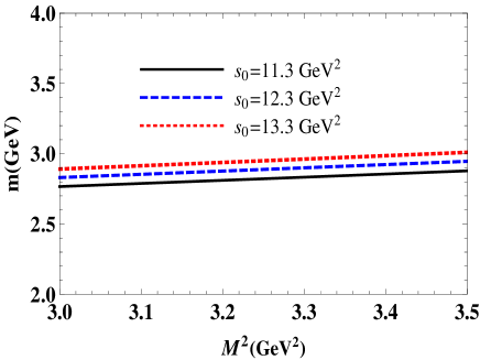
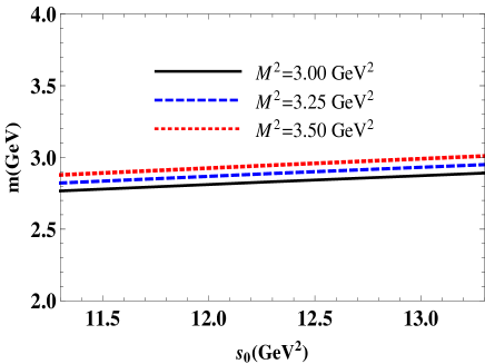
Figure 1: The mass $m$ of the tetraquark $X_{1}$ as a function of the Borel parameter $M^{2}$ (left panel), and as a function of the continuum threshold parameter $s_{0}$ (right panel).

The continuum threshold parameter $s_{0}$ separates a ground-state contribution from effects due to higher resonances and continuum states, and $\sqrt{s_{0}}$ has to be smaller than the mass $m^{\ast}$ of the first excitation of $X_{1}$. The self-consistent analysis implies that a difference $m-\sqrt{s_{0}}$ should be around of $m^{\ast}-m$. The mass gap $\sqrt{s_{0}}-m\approx(500-600)~{}\mathrm{MeV}$ fixed in the present work can be considered as a reasonable estimate $m^{\ast}\approx(m+500)~{}\mathrm{MeV}$ for the tetraquark $X_{1}$.

In Fig. 1 (left panel), we display the sum rule’s results for the mass as a function of $M^{2}$, where one can see a residual dependence of $m$ on the Borel parameter. A sensitivity of $m$ to the continuum threshold parameter $s_{0}$ is depicted in right panel of this figure.

Obtained prediction for the mass of the state $X_{1}$ is compatible with the LHCb data given in Eq. (1). But this information is not enough to make a reliable conclusion about diquark-antidiquark structure of $X_{1}$. For this purpose, we have to compute the full width $\Gamma_{\mathrm{full}}$ of the tetraquark $X_{1}$, and compare it with the relevant LHCb data. Only together the parameters $m$ and $\Gamma_{\mathrm{full}}$ can confirm or not the assumption about the nature of $X_{1}$.

III Partial widths of the decays $X_{1}\rightarrow D^{-}K^{+}$ and $X_{1}\rightarrow\overline{D}^{0}K^{0}$

The full width of the tetraquark $X_{1}$ is the sum of partial widths of its different decay channels. The resonance $X_{1}$ was observed in the $D^{-}K^{+}$ mass distribution, therefore we consider the process $X_{1}\rightarrow D^{-}K^{+}$ as its main decay channel. There is also another channel $X_{1}\rightarrow\overline{D}^{0}K^{0}$, which contributes to full width of $X_{1}$. It is worth noting that these two decays are $P$-wave processes. In $S$-wave the tetraquark $X_{1}$ may decay to a pair of either vector and scalar or axial-vector and pseudoscalar $D$ and $K$ mesons. Therefore, it is not difficult to fix possible $S$-wave channels of $X_{1}$. Thus, decays to meson pairs $\overline{D}_{1}(2420)^{0}K^{0}$, $\overline{D}_{0}^{\ast}(2400)^{0}K^{*}(892)^{0}$, $\overline{D}^{0}K_{1}(1270)^{0},$ $D^{-}K_{1}(1270)^{+}$ and a few other processes would be such channels. Threshold $2919~{}\mathrm{MeV}$ for production of a pair $\overline{D}_{1}(2420)^{0}K^{0}$ is very close to the mass of the resonance $X_{1}$, and is lowest one among listed decays. But even this threshold exceeds the mass of $X_{1}$ making kinematically forbidden the decay $X_{1}\rightarrow\overline{D}_{1}(2420)^{0}K^{0}$ and other $S$-wave processes.

In this section, we investigate the strong decay $X_{1}\rightarrow D^{-}K^{+}$ and calculate its partial width. Here, we provide details of these calculations, but will write down only final predictions for the second channel $X_{1}\rightarrow\overline{D}^{0}K^{0}$.

The width of the decay $X_{1}\rightarrow D^{-}K^{+}$ is determined by the strong coupling $g_{1}$ corresponding to the vertex $X_{1}D^{-}K^{+}$. We compute $g_{1}$ using the QCD light-cone sum rule method Balitsky:1989ry ; Belyaev:1994zk and technical tools known as a soft-meson approximation Ioffe:1983ju . Starting quantity in this method is the correlation function

$$\Pi_{\mu}(p,q)=i\int d^{4}xe^{ipx}\langle K(q)|\mathcal{T}\{J^{D}(x)J_{\mu}^{{\dagger}}(0)\}|0\rangle,$$ (17)

where by $K$ and $D$ we denote the mesons $K^{+}$ and $D^{-}$, respectively. In the correlation function $\Pi_{\mu}(p,q)$, the interpolating current $J_{\mu}(x)$ is given by Eq. (3). For $J^{D}(x)$ we use

$$J^{D}(x)=\overline{c}_{l}(x)i\gamma_{5}d_{l}(x),$$ (18)

where $l$ is the color index.

The function $\Pi_{\mu}(p,q)$ has to be rewritten in terms of the physical parameters of the initial and final particles involved into the decay. By taking into account the ground states in the $D$ and $X_{1}$ channels, we get

$$\Pi_{\mu}^{\mathrm{Phys}}(p,q) = \frac{\langle 0|J^{D}|D\left(p\right)\rangle}{p^{2}-m_{D}^{2}}\langle D\left(p\right)K(q)|X_{1}(p^{\prime})\rangle$$ (19)

$$\times\frac{\langle X_{1}(p^{\prime})|J_{\mu}^{\dagger}|0\rangle}{p^{\prime 2}-m^{2}}+\cdots,$$

where $p$, $q$ and $p^{\prime}=p+q$ are the momenta of the particles $D$, $K$, and $X_{1}$, respectively. In Eq. (19) $m_{D}$ is the mass of $D^{-}$ meson, and the ellipses refer to contributions of higher resonances and continuum states in the $D$ and $X_{1}$ channels.

To continue calculations of $\Pi_{\mu}^{\mathrm{Phys}}(p,q)$, we introduce the matrix elements

$$\langle 0|J^{D}|D\rangle=\frac{f_{D}m_{D}^{2}}{m_{c}},\ \langle X_{1}(p^{\prime})|J_{\mu}^{\dagger}|0\rangle=fm\epsilon_{\mu}^{\ast},$$

$$\langle D\left(p\right)K(q)|X_{1}(p^{\prime})\rangle=g_{1}p\cdot\epsilon.$$ (20)

In expressions above $f_{D}\,$ is decay constant of the meson $D^{-}$. Having inserted these matrix elements into expression of the correlation function, we get for $\Pi_{\mu}^{\mathrm{Phys}}(p,q)$

$$\Pi_{\mu}^{\mathrm{Phys}}(p,q)=\frac{g_{1}f_{D}fm_{D}^{2}}{2m_{c}m(p^{2}-m_{D}^{2})(p^{\prime 2}-m^{2})}$$

$$\times\left[\left(m_{D}^{2}-m_{K}^{2}-m^{2}\right)p_{\mu}+\left(m^{2}+m_{D}^{2}-m_{K}^{2}\right)q_{\mu}\right]+\cdots,$$

(21)

with $m_{K}$ being the mass of the $K^{+}$ meson. The function $\Pi_{\mu}^{\mathrm{Phys}}(p,q)$ contains two structures proportional to $p_{\mu}$ and $q_{\mu}$, respectively. Both of them can be used to derive the sum rule for the strong coupling $g_{1}$. In what follows, we work with the structure $\sim q_{\mu}$ and corresponding invariant amplitude $\Pi^{\mathrm{Phys}}(p^{2})$.

We also have to compute $\Pi_{\mu}(p,q)$ by means of the quark propagators, and find the QCD side of the sum rule. Contractions of corresponding quark and antiquark fields in Eq. (17) yield

$$\Pi_{\mu}^{\mathrm{OPE}}(p,q) = \int d^{4}xe^{ipx}\varepsilon\widetilde{\varepsilon}\left[\gamma_{5}\widetilde{S}_{d}^{lb}(x){}\gamma_{5}\right.\left.\widetilde{S}_{c}^{ml}(-x){}\gamma_{\mu}\gamma_{5}\right]_{\alpha\beta}$$ (22)

$$\times\langle K(q)|\overline{u}_{\alpha}^{c}(0)s_{\beta}^{n}(0)|0\rangle,$$

where $\alpha$ and $\beta$ are the spinor indexes.

The function $\Pi^{\mathrm{OPE}}(p,q)$ contains local matrix elements of the quark operator $\overline{u}s$ sandwiched between the vacuum and $K$ meson. After some manipulations $\langle K(q)|\overline{u}_{\alpha}^{c}(0)s_{\beta}^{n}(0)|0\rangle$ can be expressed in terms of the $K$ meson local matrix elements. To this end, $\overline{u}(0)s(0)$ should be expanded over the full set of Dirac matrices $\Gamma^{J}$ and projected onto the color-singlet states

$$\overline{u}_{\alpha}^{c}(0)s_{\beta}^{n}(0)\rightarrow\frac{1}{12}\delta^{cn}\Gamma_{\beta\alpha}^{J}\left[\overline{u}(0)\Gamma^{J}s(0)\right],$$ (23)

where

$$\Gamma^{J}=\mathbf{1},\ \gamma_{5},\ \gamma_{\mu},\ i\gamma_{5}\gamma_{\mu},\ \sigma_{\mu\nu}/\sqrt{2}.$$ (24)

Then colorless operators $\overline{u}(0)\Gamma^{J}s(0)$ give rise to matrix elements of the $K$ meson.

The expression (22) demonstrates a difference between vertices of ordinary mesons and ones composed of a tetraquark and two conventional mesons. Thus, the vertices of ordinary mesons contain non-local matrix elements $\overline{q}_{1}(x)\Gamma^{J}q_{2}(0)$ which are connected with distribution amplitudes (DAs) of a final-state meson. In the case under consideration, instead of DAs of the $K$ meson, $\Pi^{\mathrm{QCD}}(p,q)$ depends on its local matrix elements. This difference is generated by the structure of the interpolating current $J_{\mu}(x)$, which is built of four quark fields at the same space-time point. Therefore, after contracting relevant quark fields in $\Pi^{\mathrm{QCD}}(p,q)$ remaining two quarks of $X_{1}$ constitute local matrix elements of the $K$ meson. As a result, standard integrals over DAs reduce to overall normalization factors. In the context of the LCSR method this is possible in the limit $q\rightarrow 0$, when the light-cone expansion is replaced by the short-distant one Belyaev:1994zk . In this approximation $p=p^{\prime}$ and invariant amplitudes $\Pi^{\mathrm{Phys}}(p^{2})$ and $\Pi^{\mathrm{OPE}}(p^{2})$ depend only on one variable $p^{2}$. The limit $q\rightarrow 0$ is known as the soft-meson approximation to full light-cone expressions. For our purposes important is the observation made in Ref. Belyaev:1994zk : the soft-meson approximation and full LCSR treatment of the conventional mesons’ vertices lead to results, which are very close to each other.

It is clear, that in this approximation the QCD side of the LCSR becomes simpler than in its full version. But soft-meson approach gives rise to complications in the phenomenological side of the sum rule. Thus, in the soft limit we get for the amplitude $\Pi^{\mathrm{Phys}}(p^{2})$

$$\Pi^{\mathrm{Phys}}(p^{2}) = g_{1}\frac{f_{D}fm_{D}^{2}}{2mm_{c}(p^{2}-\widetilde{m}^{2})^{2}}$$ (25)

$$\times\left(2\widetilde{m}^{2}-m_{K}^{2}\right)+\cdots,$$

where $\widetilde{m}^{2}=(m^{2}+m_{D}^{2})/2$. This amplitude contains the double pole at $p^{2}=\widetilde{m}^{2}$, and its Borel transformation is given by the formula

$$\Pi^{\mathrm{Phys}}(M^{2})=g_{1}\frac{f_{D}fm_{D}^{2}}{2mm_{c}}\left(2\widetilde{m}^{2}-m_{K}^{2}\right)$$

$$\times\frac{e^{-\widetilde{m}^{2}/M^{2}}}{M^{2}}+\cdots.$$ (26)

Apart from ground-state contribution, in the soft limit the amplitude $\Pi^{\mathrm{Phys}}(M^{2})$ contains additional unsuppressed terms. In other words, double Borel transformation could not suppress all required terms. These contaminating contributions can be removed from the phenomenological side of the sum rule by applying to $\Pi^{\mathrm{Phys}}(M^{2})$ the operator Belyaev:1994zk ; Ioffe:1983ju

$$\mathcal{P}(M^{2},m^{2})=\left(1-M^{2}\frac{d}{dM^{2}}\right)M^{2}e^{m^{2}/M^{2}}.$$ (27)

Contribution of terms remained in $\Pi^{\mathrm{Phys}}(M^{2})$ after this operation can be subtracted by a usual manner. Naturally, one should act by operator $\mathcal{P}(M^{2},m^{2})$ also to QCD side of the sum rule. Then, the sum rule for the strong coupling $g_{1}$ is given by expression

$$g_{1}=\frac{2mm_{c}(2\widetilde{m}^{2}-m_{K}^{2})}{f_{D}fm_{D}^{2}}\mathcal{P}(M^{2},\widetilde{m}^{2})\Pi^{\mathrm{OPE}}(M^{2},s_{0}),$$ (28)

where $\Pi^{\mathrm{OPE}}(M^{2},s_{0})$ is Borel transformed and subtracted invariant amplitude corresponding to the structure $q_{\mu}$ in $\Pi_{\mu}^{\mathrm{OPE}}(p,q)$.

Procedures to calculate the correlation function $\Pi_{\mu}^{\mathrm{OPE}}(p,q)$ in the soft approximation were presented in Refs. Agaev:2016ijz ; Agaev:2016dev , therefore we provide only important points of these computations. First of all, after substituting the expansion (23) into Eq. (17), one carries out summations over color indices and determines local matrix elements of the $K$ meson that contribute to $\Pi_{\mu}^{\mathrm{OPE}}(p,q)$ in the soft-meson approximation. There is limited number of matrix elements that may contribute to the correlation function. They are two-particle matrix elements of twist-2 and twist-3

$$\langle 0|\overline{u}\gamma_{\mu}\gamma_{5}s|K(q)\rangle=if_{K}q_{\mu},$$

$$\langle 0|\overline{u}i\gamma_{5}s|K\rangle=\frac{f_{K}m_{K}^{2}}{m_{s}}.$$ (29)

as well as three-particle local matrix elements of $K$ meson, for an example,

$$\langle 0|\overline{u}\gamma^{\nu}\gamma_{5}igG_{\mu\nu}s|K(q)\rangle=iq_{\mu}f_{K}m_{K}^{2}\kappa_{4K},$$ (30)

where $f_{K}$ and $\kappa_{4K}$ are the decay constant and the twist-4 matrix element of the $K$ meson. It turns out that in the soft limit contributions to $\Pi_{\mu}^{\mathrm{OPE}}(p,q)$ comes from the matrix elements (29). First of them contributes to the structure $\sim q_{\mu}$, whereas $\langle 0|\overline{u}i\gamma_{5}s|K\rangle$ forms the second component of $\Pi_{\mu}^{\mathrm{OPE}}(p,q)$ proportional to $p_{\mu}$.

It has been emphasized above that, we consider the first component of the correlation function $\Pi_{\mu}^{\mathrm{OPE}}(p,q)$. For the structure $\sim q_{\mu}$ the amplitude $\Pi^{\mathrm{OPE}}(M^{2},s_{0})$ is given by the expression

$$\Pi^{\mathrm{OPE}}(M^{2},s_{0}) = -\frac{f_{K}}{48\pi^{2}}\int_{\mathcal{M}^{2}}^{s_{0}}\frac{ds(m_{c}^{2}-s)^{2}}{s}e^{-s/M^{2}}$$ (31)

$$+\Pi_{\mathrm{NP}}(M^{2}).$$

The first term in Eq. (31) given by $s$ integral is the perturbative component of $\Pi^{\mathrm{OPE}}(M^{2},s_{0})$. The nonperturbative term $\Pi_{\mathrm{NP}}(M^{2})$ has the following form

$$\Pi_{\mathrm{NP}}(M^{2})=-\frac{\langle\overline{d}d\rangle f_{K}m_{c}}{18}e^{-m_{c}^{2}/M^{2}}$$

$$+\langle\frac{\alpha_{s}G^{2}}{\pi}\rangle\frac{f_{K}m_{c}^{4}}{432M^{4}}\int_{0}^{1}\frac{dz}{z^{3}(z-1)^{3}}e^{-m_{c}^{2}/[M^{2}z(1-z)]}$$

$$+\frac{\langle\overline{d}g\sigma Gd\rangle f_{K}m_{c}^{3}}{72M^{4}}e^{-m_{c}^{2}/M^{2}}-\langle\frac{\alpha_{s}G^{2}}{\pi}\rangle\langle\overline{d}d\rangle$$

$$\times\frac{f_{K}m_{c}(m_{c}^{2}+3M^{2})\pi^{2}}{324M^{6}}e^{-m_{c}^{2}/M^{2}}+\langle\frac{\alpha_{s}G^{2}}{\pi}\rangle\langle\overline{d}g\sigma Gd\rangle$$

$$\times\frac{f_{K}m_{c}(m_{c}^{4}+7M^{2}m_{c}^{2}+8M^{4})\pi^{2}}{1296M^{10}}e^{-m_{c}^{2}/M^{2}}.$$ (32)

Parameters	Values (in $\mathrm{MeV}$ units)
$m_{D}$	$1869.65\pm 0.05$
$m_{D^{0}}$	$1864.83\pm 0.05$
$m_{K}$	$493.677\pm 0.016$
$m_{K^{0}}$	$497.611\pm 0.013$
$f_{D}=f_{D^{0}}$	$212.6\pm 0.7$
$f_{K}=f_{K^{0}}$	$155.7\pm 0.3$

Table 1: Parameters of the $D$ and $K$ mesons used in numerical analyses. Masses and decay constants of the mesons $\overline{D}^{0}$ and $K^{0}$ are denoted by $m_{D^{0}}$, $f_{D^{0}}$ and $m_{K^{0}}$, $f_{K^{0}}$, respectively.

The second decay $X_{1}\rightarrow\overline{D}^{0}K^{0}$ can be analyzed by a same manner. Difference appears in the expression of the correlation function (22), in which one should change the propagator $\widetilde{S}_{d}$ to $\widetilde{S}_{u}$, and the quark field $\overline{u}\rightarrow\overline{d}$. Related replacements $\langle\overline{d}d\rangle\rightarrow\langle\overline{u}u\rangle$, $\langle\overline{d}g\sigma Gd\rangle\rightarrow\langle\overline{u}g\sigma Gu\rangle$ in Eq. (32) do not change numerical predictions.

Besides the vacuum condensates, Eq. (28) contains masses and decay constants of the final-state mesons $D^{-}$ and $K^{+}$. Their spectroscopic parameters, as well as parameters of the mesons $\overline{D}^{0}$ and $K^{0}$ are collected in Table 1: All of them are borrowed from Ref. PDG:2020 .

Our analysis demonstrates that working windows (15) used in the mass calculations satisfy necessary constraints on $M^{2}$ and $s_{0}$ imposed in the case of the decay process. Therefore, in computations of $\Pi^{\mathrm{OPE}}(M^{2},s_{0})$ we vary $M^{2}$ and $s_{0}$ within limits (15).

For $g_{1}$ numerical calculations yield

$$g_{1}=8.6\pm 1.1.$$ (33)

The partial width of the decay $X_{1}\rightarrow D^{-}K^{+\text{ }}$ is determined by the simple formula

$$\Gamma_{\mathrm{A}}\left[X_{1}\rightarrow D^{-}K^{+}\right]=\frac{g_{1}^{2}\lambda^{3}\left(m,m_{D},m_{K}\right)}{24\pi m^{2}},$$ (34)

where

$$\lambda\left(a,b,c\right) = \frac{1}{2a}\left[a^{4}+b^{4}+c^{4}\right.$$ (35)

$$\left.-2\left(a^{2}b^{2}+a^{2}c^{2}+b^{2}c^{2}\right)\right]^{1/2}.$$

Then it is not difficult to find that

$$\Gamma_{\mathrm{A}}\left[X_{1}\rightarrow D^{-}K^{+}\right]=(46\pm 9)~{}\mathrm{MeV}.$$ (36)

The strong coupling and partial width of the second process $X_{1}\rightarrow\overline{D}^{0}K^{0}$ can be obtained by the same way:

$$g_{2}=8.7\pm 1.1,$$

$$\Gamma_{\mathrm{B}}\left[X_{1}\rightarrow\overline{D}^{0}K^{0}\right]=(47\pm 9)~{}\mathrm{MeV}.$$ (37)

Differences between couplings $g_{1}$ and $g_{2}$, and partial widths of two channels originate from parameters of the final-state mesons, therefore are very small. Extracted predictions for $\Gamma_{\mathrm{A}}$ and $\Gamma_{\mathrm{B}}$ allow us to evaluate the full width of the tetraquark $X_{1}$

$$\Gamma_{\mathrm{full}}=(93\pm 13)~{}\mathrm{MeV}.$$ (38)

Confronting the sum rule’s prediction for $\Gamma_{\mathrm{full}}$ with the LHCb data, one sees that $\Gamma_{\mathrm{full}}$ is smaller than the measured value in Eq. (1). Nevertheless, within ambiguities of theoretical calculations, $\Gamma_{\mathrm{full}}$ is in a reasonable agreement with $\Gamma_{1}$.

IV Discussion and concluding notes

In the present paper, we have investigated the new resonance $X_{1}$ observed recently by the LHCb collaboration. We have modeled $X_{1}$ as the vector diquark-antidiquark state $[ud][\overline{c}\overline{s}]$ and computed its mass and full decay width $\Gamma_{\mathrm{full}}$. The mass of the state $X_{1}=[ud][\overline{c}\overline{s}]$ has been evaluated in the framework of the QCD two-point sum rule approach. Obtained prediction for $m$ nicely agrees with the LHCb data, and may be considered as arguments in favor of diquark-antidiquark structure of the resonance $X_{1}$.

We have evaluated the full width of the tetraquark $X_{1}$ as well. To this end, we have analyzed its two $P$-wave decay modes $X_{1}\rightarrow D^{-}K^{+}$ and $X_{1}\rightarrow\overline{D}^{0}K^{0}$. Strong couplings corresponding to vertices $X_{1}D^{-}K^{+}$ and $X_{1}\overline{D}^{0}K^{0}$ have been calculated by employing the LCSR method and soft-meson approximation. It has been found that their widths do not differ from each another, and these channels form the full width of the tetraquark $X_{1}$ on equal footing. The result obtained for $\Gamma_{\mathrm{full}}$ is compatible with LHCb measurements.

The mass of $X_{1}$ was calculated in the context of the sum rule method also in Ref. Chen:2020aos . The prediction $m=2940_{-110}^{+130}~{}\mathrm{MeV}$ obtained there is somewhat larger than our result, but within theoretical errors still agrees with the LHCb data. Relatively large output for $m$ is presumably connected with a form of interpolating current and accuracy of performed calculations.

Production of the structures $X_{0}$ and $X_{1}$ in $B$ meson’s weak decays were analyzed in Ref. Burns:2020xne . The central idea and main conclusion of this work is that production of $X_{0,1}$ is dominated by color-favored processes. It was also argued that competing models for $X_{0,1}$ can be unambiguously discriminated due to differences in features of their production and decay mechanisms. Similar problems were addressed in articles Bondar:2020eoa ; Chen:2020eyu as well.

The resonances $X_{0,1}$ are neutral structures, but may have charged partners Burns:2020xne . In our view, more interesting is a case of exotic mesons built of  four quarks of different flavors and carrying two units of the electric charge. We are going now to consider production of doubly charged tetraquarks $Z^{++}=[uc][\overline{s}\overline{d}]$ in $B$ decays. In Ref. Agaev:2017oay we investigated scalar, pseudoscalar and axial-vector states $Z_{\overline{c}s}=[sd][\overline{u}\overline{c}]$ with the charge $-2|e|$, and computed their masses and decay widths. Tetraquarks $Z^{++}$  are positively charged partners of $Z_{\overline{c}s}$ and should have the same masses. Therefore, in our analysis of $Z^{++}$, we use results presented in Ref. Agaev:2017oay . Then scalar and axial-vector states $Z_{\mathrm{S}}^{++}$ and $Z_{\mathrm{AV}}^{++}$ should have the masses $2628_{-153}^{+166}~{}\mathrm{MeV}$ and $2826_{-157}^{+134}~{}\mathrm{MeV}$, respectively. We did not calculate parameters of vector tetraquark $Z_{\overline{c}s}$, but can safely suppose that $Z_{\mathrm{V}}^{++}$ is heavier than $Z_{\mathrm{S}}^{++}$ and its mass is comparable with mass of $Z_{\mathrm{AV}}^{++}$. The scalar particle $Z_{\mathrm{S}}^{++}$ in $S$-wave can decay to mesons $D_{s}^{+}\pi^{+}$ and $D^{+}K^{+}$. The vector tetraquark $Z_{\mathrm{V}}^{++}$ in $P$-wave has the same decay modes. In other words, decays to ordinary meson pairs $D_{s}^{+}\pi^{+}$ and $D^{+}K^{+}$ are kinematically allowed processes for both $Z_{\mathrm{S}}^{++}$ and $Z_{\mathrm{V}}^{++}$.

The structures $X_{0}$ and $X_{1}$ were discovered in the process $B^{+}\rightarrow D^{+}X\rightarrow D^{+}D^{-}K^{+}$ and fixed in the $D^{-}K^{+}$ invariant mass distribution. This decay runs through color-favored and color-suppressed topologies labeled in Ref. Burns:2020xne as $(1)$ and $(2)$, respectively. It is not difficult to see that weak decays of $B^{+}$ with the same topologies may generate the process $B^{+}\rightarrow D^{-}Z^{++}\rightarrow D^{-}D^{+}K^{+}$ as well. As a result, doubly charged scalar and vector tetraquarks may manifest themselves in the invariant mass distribution of the pair $D^{+}K^{+}$. There is intriguing possibility to observe doubly charged four-quark structures in decay $B^{+}\rightarrow D^{-}D^{+}K^{+}$: It is quite possible, that decays through $X$ and $Z^{++}$ are competing mechanisms in this process. Other $B$ meson channels with $D_{s}^{+}\pi^{+}$ pairs in final-state, perhaps, are suitable for such studies as well. Experimental data collected by the LHCb collaboration would hopefully be enough to perform relevant investigations.

As is seen, there are different interpretations of new structures discovered recently by the LHCb collaboration in decay $B^{+}\rightarrow D^{+}D^{-}K^{+}$. Experimental data do not raise doubts about existence of the resonance-like enhancements $X_{0}$ and $X_{1}$ in the $D^{-}K^{+}$ mass distribution. Till now $X_{0}$ and $X_{1}$ were examined as the hadronic molecules, diquark-antidiquark systems, and rescattering effects. In our view, the same decay  $B^{+}\rightarrow D^{+}D^{-}K^{+}$ may also be used to see doubly charged resonances. Additional experimental and theoretical studies are evidently required to clarify all these problems.

References

- (1) R. Aaij et al. [LHCb], Phys. Rev. Lett. 125, 242001 (2020).
- (2) R. Aaij et al. [LHCb], Phys. Rev. D 102, 112003 (2020).
- (3) M. Karliner and J. L. Rosner, Phys. Rev. D 102, 094016 (2020).
- (4) Z. G. Wang, Int. J. Mod. Phys. A 35, 2050187 (2020).
- (5) H. X. Chen, W. Chen, R. R. Dong and N. Su, Chin. Phys. Lett. 37, 101201 (2020).
- (6) M. Z. Liu, J. J. Xie and L. S. Geng, Phys. Rev. D 102, 091502 (2020).
- (7) R. Molina and E. Oset, Phys. Lett. B 811, 135870 (2020).
- (8) M. W. Hu, X. Y. Lao, P. Ling and Q. Wang, arXiv:2008.06894 [hep-ph].
- (9) X. G. He, W. Wang and R. Zhu, Eur. Phys. J. C 80, 1026 (2020).
- (10) X. H. Liu, M. J. Yan, H. W. Ke, G. Li and J. J. Xie, arXiv:2008.07190 [hep-ph].
- (11) Q. F. Lu, D. Y. Chen and Y. B. Dong, Phys. Rev. D 102, 074021 (2020).
- (12) J. R. Zhang, arXiv:2008.07295 [hep-ph].
- (13) Y. Huang, J. X. Lu, J. J. Xie and L. S. Geng, Eur. Phys. J. C 80, 973 (2020).
- (14) Y. Xue, X. Jin, H. Huang and J. Ping, arXiv:2008.09516 [hep-ph].
- (15) G. Yang, J. Ping and J. Segovia, arXiv:2101.04933 [hep-ph].
- (16) T. W. Wu, M. Z. Liu and L. S. Geng, Phys. Rev. D 103, L031501 (2021).
- (17) L. M. Abreu, Phys. Rev. D 103, 036013 (2021).
- (18) G. J. Wang, L. Meng, L. Y. Xiao, M. Oka and S. L. Zhu, Eur. Phys. J. C 81, 188 (2021).
- (19) C. J. Xiao, D. Y. Chen, Y. B. Dong and G. W. Meng, Phys. Rev. D 103, 034004 (2021).
- (20) X. K. Dong and B. S. Zou, arXiv:2009.11619 [hep-ph].
- (21) T. J. Burns and E. S. Swanson, Phys. Rev. D 103, 014004 (2021).
- (22) A. E. Bondar and A. I. Milstein, JHEP 12, 015 (2020).
- (23) Y. K. Chen, J. J. Han, Q. F. Lü, J. P. Wang and F. S. Yu, Eur. Phys. J. C 81, 71 (2021).
- (24) R. M. Albuquerque, S. Narison, D. Rabetiarivony and G. Randriamanatrika, Nucl. Phys. A 1007, 122113 (2021).
- (25) H. X. Chen, arXiv:2103.08586 [hep-ph].
- (26) S. S. Agaev, K. Azizi and H. Sundu, arXiv:2008.13027 [hep-ph].
- (27) S. S. Agaev, K. Azizi and H. Sundu, Phys. Rev. D 93, 094006 (2016).
- (28) W. Chen, H. X. Chen, X. Liu, T. G. Steele and S. L. Zhu, Phys. Rev. Lett. 117, 022002 (2016).
- (29) S. S. Agaev, K. Azizi and H. Sundu, Eur. Phys. J. C 78, 141 (2018).
- (30) M. A. Shifman, A. I. Vainshtein and V. I. Zakharov, Nucl. Phys. B 147, 385 (1979).
- (31) M. A. Shifman, A. I. Vainshtein and V. I. Zakharov, Nucl. Phys. B 147, 448 (1979).
- (32) H. X. Chen, W. Chen, X. Liu and S. L. Zhu, Phys. Rept. 639, 1 (2016).
- (33) H. X. Chen, W. Chen, X. Liu, Y. R. Liu and S. L. Zhu, Rept. Prog. Phys. 80, 076201 (2017).
- (34) R. M. Albuquerque, J. M. Dias, K. P. Khemchandani, A. Martínez Torres, F. S. Navarra, M. Nielsen and C. M. Zanetti, J. Phys. G 46, 093002 (2019).
- (35) S. S. Agaev, K. Azizi and H. Sundu, Turk. J. Phys. 44, 95 (2020).
- (36) Y. Kondo, O. Morimatsu and T. Nishikawa, Phys. Lett. B 611, 93 (2005).
- (37) S. H. Lee, H. Kim and Y. Kwon, Phys. Lett. B 609, 252 (2005).
- (38) Z. G. Wang, Int. J. Mod. Phys. A 30, 1550168 (2015).
- (39) S. S. Agaev, K. Azizi, B. Barsbay and H. Sundu, Nucl. Phys. B 939, 130 (2019).
- (40) H. Sundu, S. S. Agaev and K. Azizi, Eur. Phys. J. C 79, 215 (2019).
- (41) B. L. Ioffe, Prog. Part. Nucl. Phys. 56, 232 (2006).
- (42) S. Narison, Nucl. Part. Phys. Proc. 270-272, 143 (2016).
- (43) I. I. Balitsky, V. M. Braun and A. V. Kolesnichenko, Nucl. Phys. B 312, 509 (1989).
- (44) V. M. Belyaev, V. M. Braun, A. Khodjamirian and R. Ruckl, Phys. Rev. D 51, 6177 (1995).
- (45) B. L. Ioffe and A. V. Smilga, Nucl. Phys. B 232, 109 (1984).
- (46) S. S. Agaev, K. Azizi and H. Sundu, Phys. Rev. D 93, 114007 (2016).
- (47) S. S. Agaev, K. Azizi and H. Sundu, Phys. Rev. D 93, 074002 (2016).
- (48) P. A. Zyla et al. [Particle Data Group], Prog. Theor. Exp. Phys. 2020, 083C01 (2020).