Variability of newly identified B-type stars observed by Kepler

Abstract

Recent re-determination of stellar atmospheric parameters for a sample of stars observed during the Kepler mission allowed to enlarge the number of Kepler B-type stars. We present the detailed frequency analysis for all these objects. All stars exhibit pulsational variability with maximum amplitudes at frequencies corresponding to high-order g modes. Peaks that could be identified with low-order p/g modes are also extracted for a few stars. We identified some patters in the oscillation spectra that can be associated with the period spacings that can result from the asymptotic nature of the detected pulsational modes. We also tentatively confront the observed oscillation characteristics with predictions from linear nonadiabatic computations of stellar pulsations. For high-order g modes the traditional approximation was employed to include the effects of rotation on the frequency values and mode instability.

1 Introduction

B-type stars, compared to the less massive stars, are relatively rare objects. Nevertheless, they are very important ingredients of stellar populations. They enrich interstellar medium in heavy elements as well as nitrogen and carbon and, due to their high masses, determine the structure of stellar systems. Unfortunately, some aspects of their evolution, especially element mixing processes and angular momentum transfer, are still poorly understood.

In the beginning of previous century, it has been found that some B-type stars exhibit photometric and spectroscopic variability (Frost, 1902; Guthnick, 1913) that was associated with radial and non-radial pulsations (Ledoux, 1951). These pulsations are driven on the local opacity increase caused by iron group elements, (so called Z-bump, Moskalik & Dziembowski, 1992; Cox et al., 1992; Dziembowski & Pamiatnykh, 1993; Dziembowski et al., 1993; Gautschy & Saio, 1993).

B-type stars that pulsate in low-overtone p and g modes are called $\beta$ Cephei (e.g.  Stankov & Handler, 2005), whereas B-type stars pulsating in high-overtone g modes are called Slowly Pulsating B-type stars (SPB, Waelkens, 1991), and those exhibiting both types of pulsations are called $\beta$ Cep/SPB hybrid pulsators (e.g.  Jerzykiewicz et al., 2005; Handler et al., 2006; Chapellier et al., 2006; Balona et al., 2011).

Apart from uncertainties mentioned in the first paragraph, asteroseismic studies of B-type pulsators e.g. Walczak et al. (2017a); Walczak et al. (2017b); Daszyńska-Daszkiewicz et al. (2017a, b); Szewczuk & Daszyńska-Daszkiewicz (2018); Walczak et al. (2019) suggest that stellar opacities still need some revision. In particular, a huge increase of opacity is necessary to excite high-order g modes in early B-type stars (Salmon et al., 2012; Daszyńska-Daszkiewicz et al., 2017b). Theoretical work by Hui-Bon-Hoa & Vauclair (2018) showed, that including diffusion of heavy elements does cause the accumulation of iron and nickel in the vicinity of driving zone in massive stars, which significantly increases the opacity in these layers.

In the recent decade, the space born missions: MOST, CoRoT Kepler, K2, BRITE, TESS have provided high precision photometric data. It has became obvious that variability is common among B-type stars (e.g. Balona et al., 2011; McNamara et al., 2012), although there are known, up to the level of available photometric precision, constant stars (eg. KIC 11817929, Balona et al., 2011).

Table 1: Atmospheric parameters and available Kepler data for our sample of stars. The columns contain sequentially: our ID number, Kepler number, effective temperature, $T_{\mathrm{eff}}$, gravity, $\log g$, projected rotational velocity, $V\sin i$ and available Kepler quarters. The stellar parameters are taken from H19.

#	KIC ID	$T_{\mathrm{eff}}$ (K)	$\log g$ (dex)	$V\sin i$ (km s-1)	Kepler data
1	1430353	17000(2000)	3.30(0.27)	210(26)	Q0-Q17
2	3459297	13100(600)	3.61(0.14)	123(12)	Q0-Q5; Q7-Q9; Q11-Q13; Q15-Q17
3	3839930	16950(650)	4.18(0.13)	51(6)	Q0-Q2; Q4-Q5; Q7-Q9; Q11-Q13; Q15-Q17
4	3862353	14000(1000)	3.71(0.18)	64(15)	Q2-Q3; Q7-Q9
5	4077252	12100(900)	3.51(0.22)	65(23)	Q0-Q5; Q7-Q9; Q11-Q13; Q15-Q17
6	4936089	12250(600)	4.05(0.18)	48(7)	Q1-Q5; Q7-Q9; Q11-Q13; Q15-Q17
7	4939281	17500(1000)	3.87(0.14)	115(20)	Q0-Q5; Q7-Q9; Q11-Q13; Q15-Q17
8	5477601	11950(350)	4.10(0.14)	88(11)	Q0-Q17
9	7630417	19200(1900)	3.73(0.24)	135(16)	Q1-Q17
10	8167938	13400(1000)	4.00(0.22)	70(3)	Q2-Q4; Q6-Q8; Q10-Q12; Q14-Q16
11	8264293	13150(500)	4.08(0.14)	284(13)	Q0-Q17
12	8381949	20200(2000)	3.72(0.27)	245(21)	Q0-Q17
13	8714886	18200(900)	4.10(0.14)	52(9)	Q0-Q17
14	9227988	14000(1200)	3.34(0.18)	50(3)	Q0-Q17
15	9278405	11100(200)	4.14(0.11)	110(17)	Q0-Q17
16	9468611	10750(550)	3.70(0.22)	263(30)	Q0-Q17
17	9715425	15750(1500)	3.52(0.27)	122(12)	Q0-Q17
18	9910544	12100(300)	4.10(0.14)	72(5)	Q2-Q6; Q8-Q10; Q12-Q14; Q16-Q17
19	9964614	20100(850)	3.84(0.14)	77(14)	Q0-Q6; Q8-Q10; Q12-Q14; Q16-Q17
20	10118750	10950(500)	4.27(0.22)	271(16)	Q1-Q17
21	10526294	11500(500)	4.18(0.14)	36(10)	Q1-Q17
22	10790075	11850(400)	3.63(0.14)	71(5)	Q0-Q17
23	11293898	16400(1000)	3.79(0.18)	355(35)	Q0-Q17
24	11360704	16500(1050)	3.72(0.14)	303(12)	Q0-Q17
25	11671923	11800(200)	4.05(0.11)	91(8)	Q0-Q17

Satellite missions dedicated to perform long and continues photometric time series opened a new window in asteroseismic studies of B-type stars. These observations have allowed for the detection of a much larger number of frequencies than was accessible from ground-based observations (e.g.  Pedersen et al., 2019). Moreover, it turned out that a vast majority of B-type pulsators, if not all, are the $\beta$ Cep/SPB hybrid pulsators. This fact has increased an opportunity of probing stellar interiors using asteroseismic tools with unprecedented precision. Unfortunately, it quickly turned out that we were dealing with a kind of failure of richness (e.g.  Szewczuk et al., 2014). We have hundreds of frequencies, but we do not know what theoretical modes correspond to them. Thus, we still have to face with the old standing problem of mode identification, i.e. determination of the mode degree $\ell$, azimuthal order $m$ and radial order $n$.

In the case of one-band photometric data the only way to determine $\ell$ and $m$ is to look for regularities in the spectrum of oscillations. One can expect some characteristic features, that are multiplets caused by rotational splitting of modes with the same $\ell$ and radial order $n$. In the case of low frequencies corresponding to high-order g modes, the asymptotic theory of oscillation predicts a regular period spacing between consecutive radial orders for a given $\ell$ and $m$ (e.g.  Tassoul, 1980; Dziembowski et al., 1993; Bouabid et al., 2013).

Up to now Kepler satellite give the best, in terms of quality and time span, photometric time series of B-type stars. The general view of oscillations of B-type stars observed by Kepler was published by Balona et al. (2011) and McNamara et al. (2012), but only the first quarters of Kepler observations were available at that time.

The patterns of regular period spacings in Kepler’s B stars were found by Pápics et al. (2014, 2015, 2017), Szewczuk & Daszyńska-Daszkiewicz (2018) and Zhang et al. (2018). Three stars, namely KIC 10526294 (Moravveji et al., 2015; Triana et al., 2015), KIC 7760680 (Moravveji et al., 2016; Szewczuk et al., 2017) and KIC 3240411 (Szewczuk & Daszyńska-Daszkiewicz, 2018), were subjects of detailed seismic analysis.

Because B-type stars in Kepler field are not numerous, any additional enlarging sample is desirable. Since effective temperatures and gravities, especially for hot stars in KIC (Kepler Input Catalogue) are not accurate and often underestimated, some B-type stars can be misclassified as cool stars (e.g.  Brown et al., 2011; Pinsonneault et al., 2012; Zhang et al., 2018). Recently Hanes et al. (2019) redetermined stellar parameters of 25 stars observed by Kepler. In most cases, Hanes et al. (2019) found that their actual effective temperatures correspond to B-type stars, whereas they were previously considered as cool stars.

The aim of this paper is to characterize oscillation properties of B-type stars listed in Hanes et al. (2019). In particular, the ultimate goal is to find regular patterns in the spectra of oscillations.

In Section 1, we give a short description of observational data and periodogram analysis. Section 3 contains results for individual stars. In Section 4 we describe red noise that was found in the data. Conclusions are summarized in Section 5. Some additional material is available in the appendix A.

2 Star sample

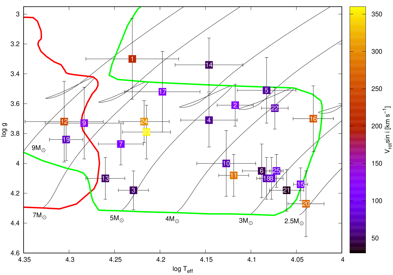
Figure 1: The position of target stars in the Kiel diagram. The stars are marked with numbers from the first column of Table 1. The values of $V\sin i$ is colour-coded. All parameters are taken from H19. Green and red lines represent domains of pulsational instability for the SPB and $\beta\,$Cep stars, respectively (Walczak et al., 2015). Modes with the degree $\ell=0,\,1,\,2$ are considered.

Here we analyze in details 25 stars listed by Hanes et al. (2019, hereafter H19). Two of these stars, KIC 10526294 and KIC 3459297 were already studied by Pápics et al. (2014, 2017) and regular period spacings were found. We reanalysed these two stars and derived very similar results. Moreover, variability of KIC 3839930, KIC 8381949, KIC 8714886, KIC 9964614 and KIC 11360704 was previously investigated by Balona et al. (2011) but only first quarters of Kepler data were used. Therefore, we performed new analysis these stars using all available data.

Stellar parameters of selected stars, as determined by H19, are given in Table 1. In Fig. 1, we show the positions of our sample stars in the Kiel diagram. The domains of pulsational instability for the $\beta$ Cephei and SPB stars are also depicted (Walczak et al., 2015). As one can see all stars are inside (within observational errors) SPB instability strip. Four of them, KIC 7630417, KIC 8381949, KIC 8714886, KIC 9964614, lie also inside $\beta$ Cep instability strip.

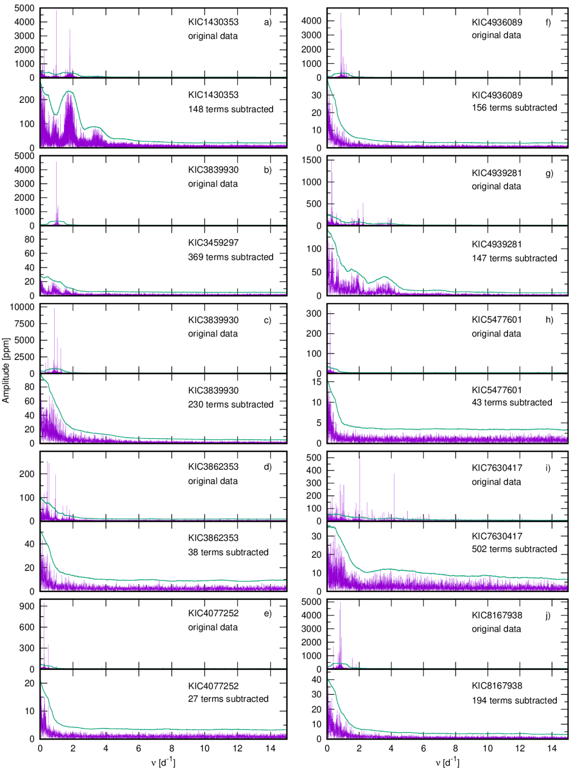
Figure 2: Fourier transforms of the original data and the data pre-whitened with all significant frequencies (the top and bottom panel for each star, respectively). The $S/N=4$ level is marked as a green line.

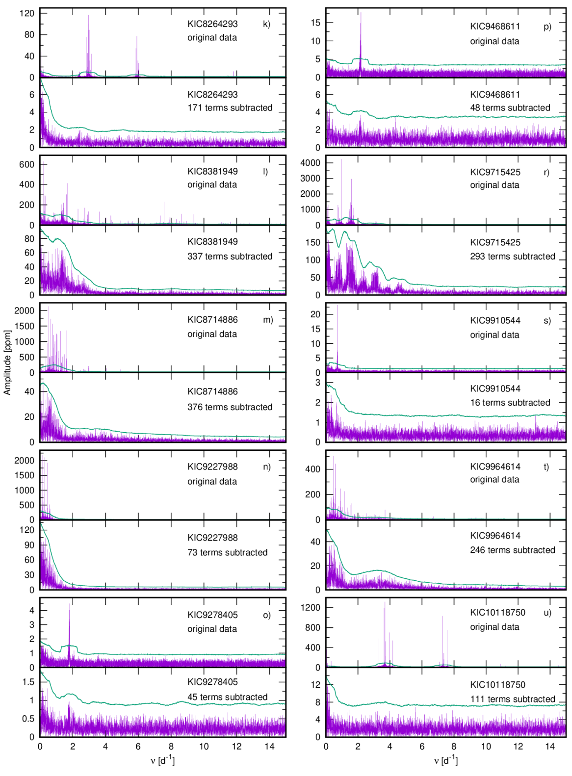
Figure 3: Continuation of Fig. 2.

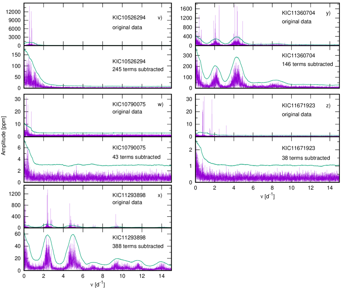
Figure 4: Continuation of Fig. 2.

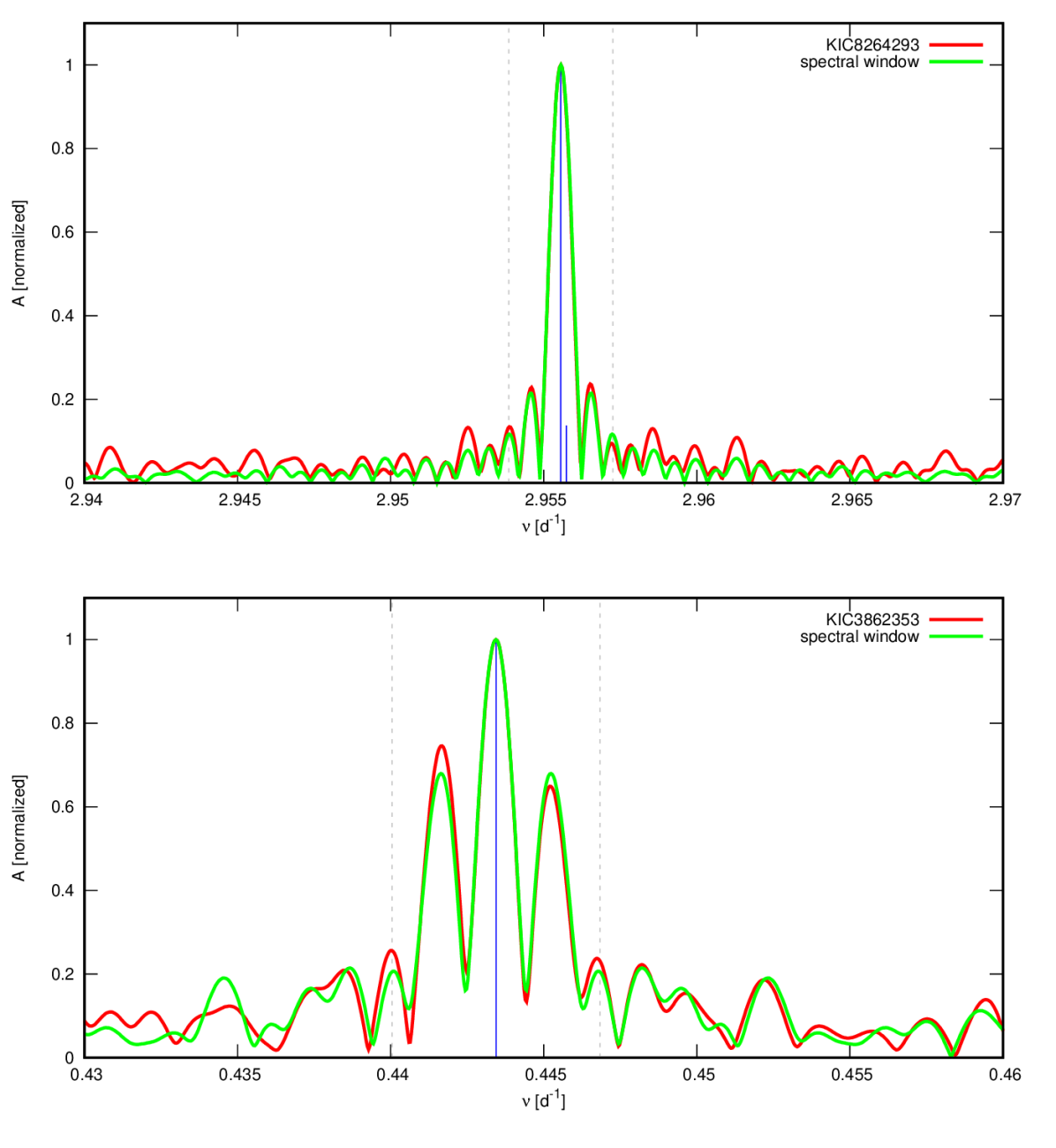
Figure 5: Normalized spectral window (green lines) and Fourier transform of original data (red lines). Results for KIC 8264293 and for KIC 3862353 are displayed in the upper and bottom panel, respectively. Spectral window is shifted to the frequency of the dominant mode. There are also shown frequencies found in our periodogram analysis that met $S/N\geq 4$ criterion (blue vertical lines). Dashed gray lines mark $2.5/T$ resolution limit around the dominant frequency.

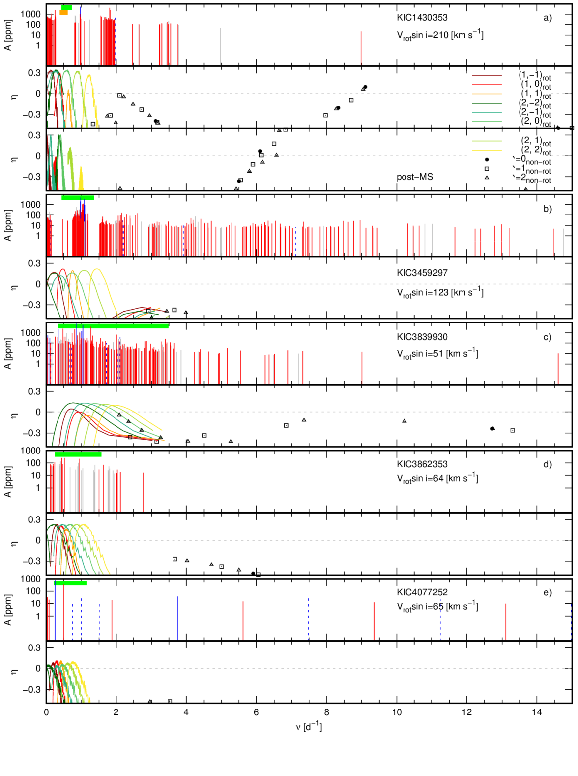
Figure 6: Top panels: All significant frequencies extracted from the observations. Independent frequencies are marked with vertical red lines and combinations with vertical gray lines. Vertical blue continuous lines indicate independent frequencies for which harmonics are present. Harmonics are marked with vertical blue dashed lines. Bands (green for main sequence models and orange for post-main sequence models, if considered) give the range of rotation frequencies allowed by $V_{\mathrm{rot}}\sin i$ and critical rotation for each star. Bottom panels: The instability parameters, $\eta$, for radial, dipole and quadruple modes in representative models of each stars (see the text for details). Coloured lines depict the values of $\eta$ calculated in the framework of the traditional approximation, whereas, black symbols depict the value of $\eta$ calculated within the zero-rotation approximation.

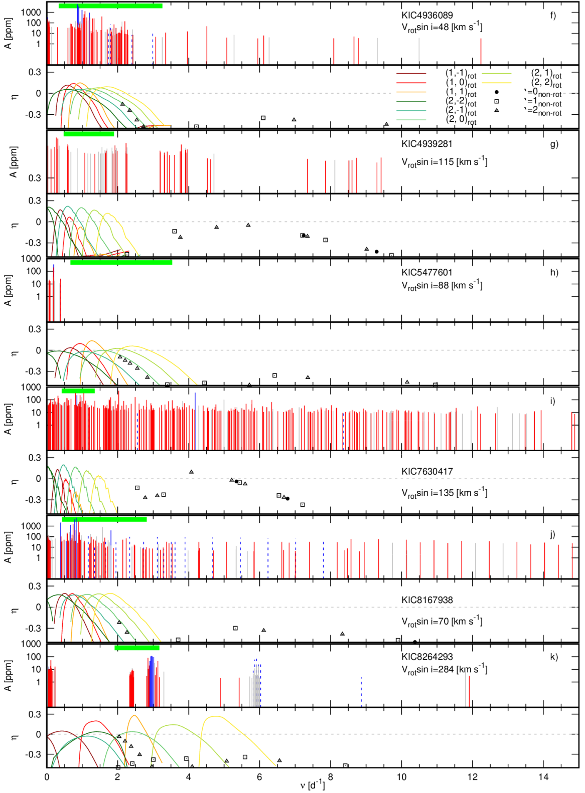
Figure 7: Continuation of Fig. 6.

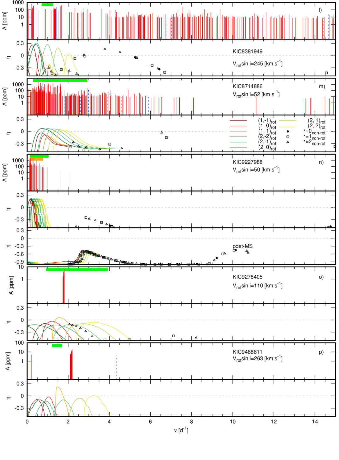
Figure 8: Continuation of Fig. 6.

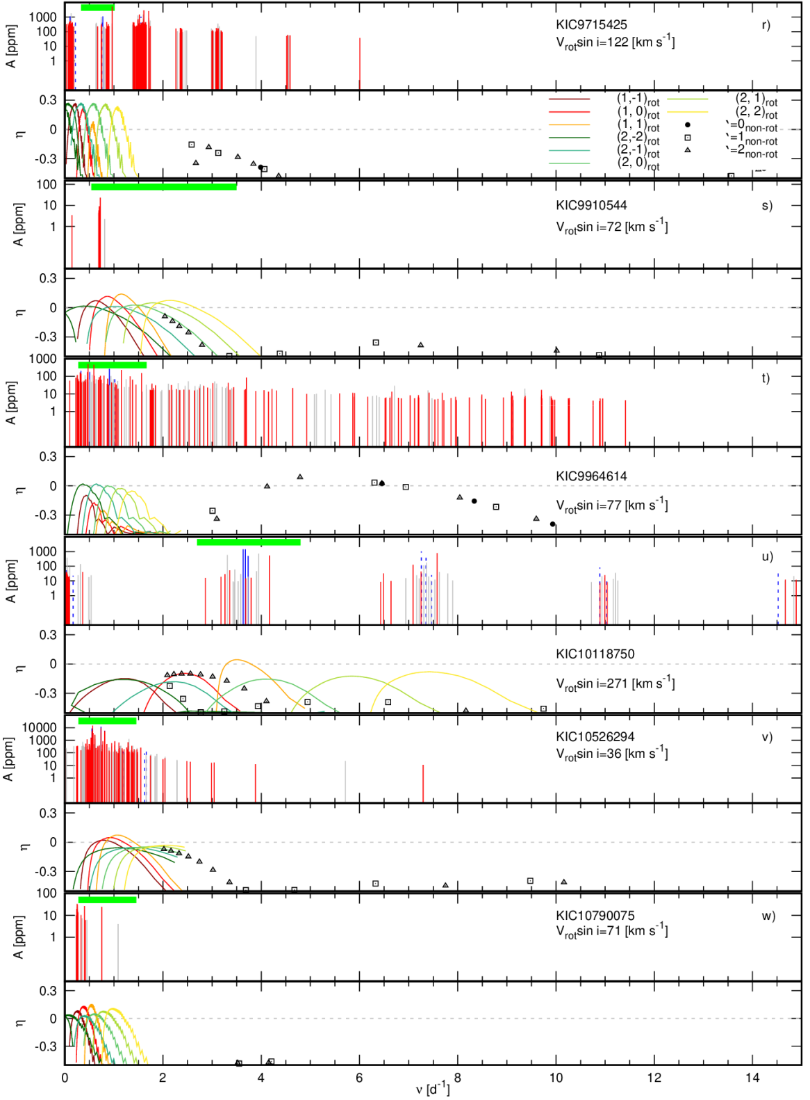
Figure 9: Continuation of Fig. 6.

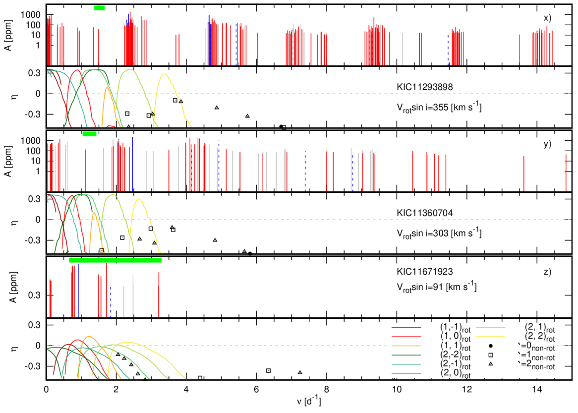
Figure 10: Continuation of Fig. 6.

2.1 Data reduction

During its main mission Kepler satellite was gathering almost continuous photometric data for 1470 days. Major gaps in the observations of some stars are caused by the failures of the individual CCD chips during mission. Available data for our targets are listed in the last column of Table 1. All these data are in public domain and are distributed in the form of prepared light curves and so-called target pixel files. Publicly available light curves were optimized for searching planets, i.e., they were extracted from the pixels that lay inside the optimal aperture that was selected to maximize the signal-to-noise ratio (S/N). It was shown (see e.g. Pápics et al., 2014) that such definition of aperture is not the best choice for extracting low frequencies from the light curves. Usually, including more pixels gives better results in the sense of long-term stability of the light curve. This is especially important in the case of long period pulsators such as the SPB stars.

Therefore, we decided to extract our own light curves from target pixel files. In general we proceeded in a similar way as in Szewczuk & Daszyńska-Daszkiewicz (2018). In the first step, for all target stars and quarters we defined customized apertures (masks) that contain all pixels with signal to noise ratio grater than 100. Next, we performed summing of the flux values within these masks and removed the obvious outliers.

An important step of the whole procedure was removing systematic trends using co-trending basis vectors (e.g.  Thompson et al., 2016). We started with five basis vectors and after an eye inspection we decided whether it was necessary to add another one. Since employing too many vectors could lead to overfitting the data, cleaning off the real astrophysical signals or adding spurious signals, this step was crucial and we paid a lot of attention to this procedure. In the majority of cases 5 basic vectors were enough but in the most extreme ones we had to use the full set of 16 basic vectors (e.g., KIC 11671923). For some stars, individual quarters had to be divided into smaller subset and analyzed separately. These steps were made with the use of PyKe 3.0 package (Still & Barclay, 2012; Vinícius et al., 2017).

Finally, once again outliers were sought and removed. Then, the quarters were divided by a second-order polynomial fit, merged and transformed into the ppm units.

2.2 Periodogram analysis

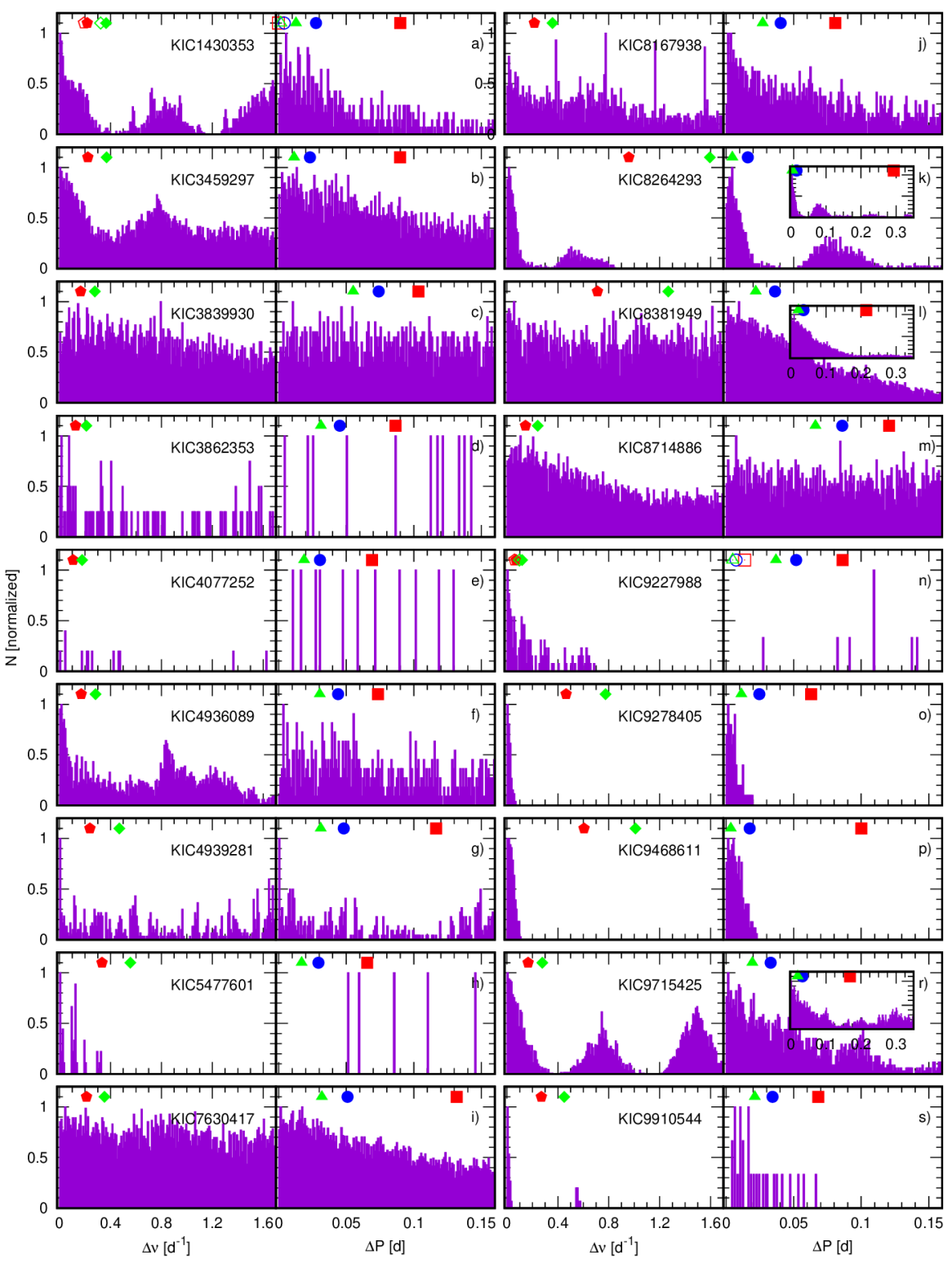
Figure 11: Normalized histograms of the differences in frequencies and periods. Red pentagons and green diamonds indicate the theoretical rotational splittings calculated for rotation rate equal to $V_{\mathrm{rot}}\sin i$ for $\ell=1$ and 2 modes, respectively. Open symbols are for post-main sequence models (if considered). Green triangles, blue circles and red squares indicate mean period spacing in representative models for dipole modes with $m=1$, 0 and $-1$, respectively. The insets show wider range of $\Delta\nu$ i $\Delta$ P if needed. See text for details.

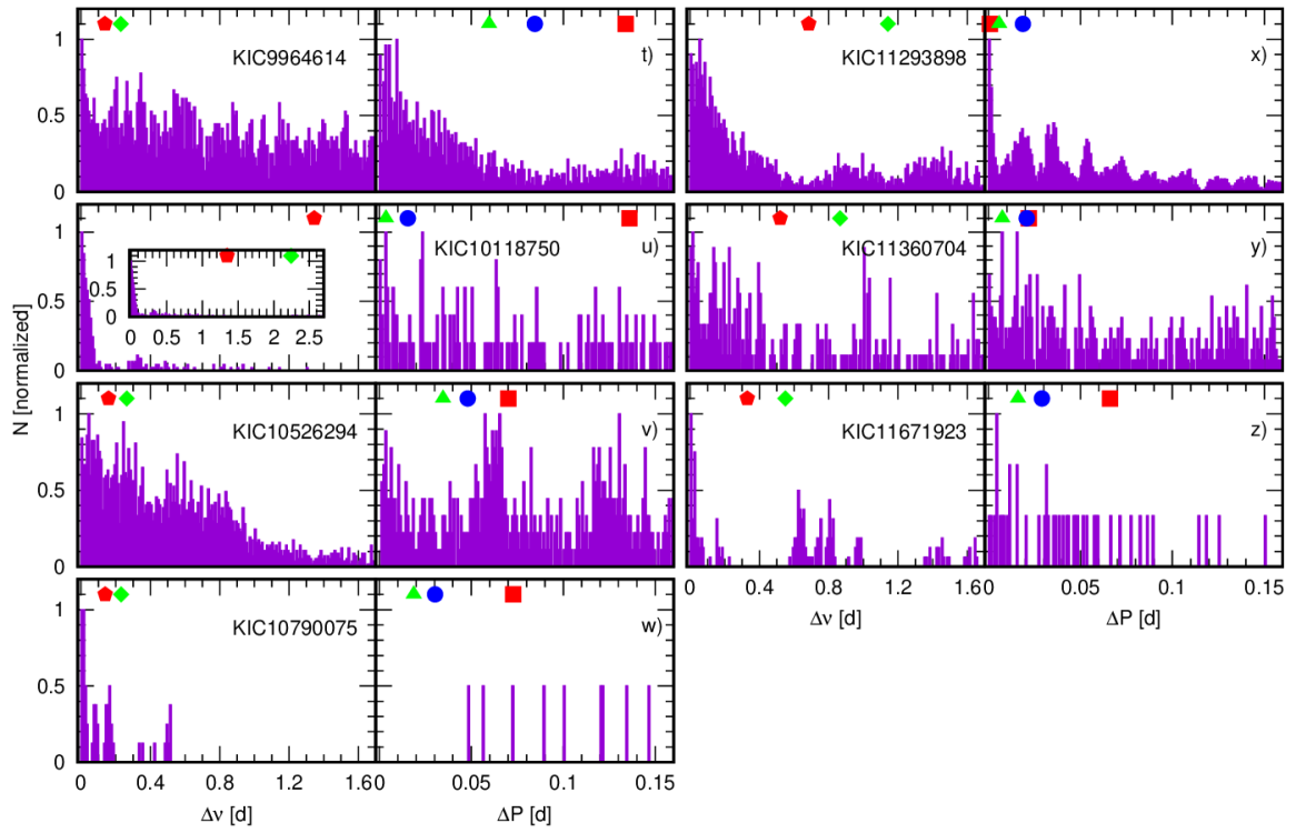
Figure 12: The continuation of Fig. 11.

In order to extract frequencies of the periodic light variability, we proceeded the standard prewhitening procedure. Amplitude periodograms were calculated up to the Nyquist frequency, i.e., to about $24.5\,\mathrm{d}^{-1}$ with the fixed resolution of $4\times 10^{-5}\,\mathrm{d^{-1}}$. As a significance criterion of a given frequency peak we chose the signal-to-noise ratio $S/N\ =4$ (Breger, 1993; Kuschnig et al., 1997). The noise was calculated as a mean amplitude in a one day window centered at this frequency before its extraction.

Light curves of the studied stars exhibit clear and complex variability (see Fig. 33 in Appendix A). The corresponding periodograms for all studied stars are shown in Figs. 2, 3 and 4. For each star we plotted in two panels, one above the other, a periodogram calculated for the original data (upper panel) and for data prewhithened for all significant frequencies (bottom panel). The number of removed terms, i.e., the number of significant frequencies, is given as well. In addition we plotted a spectral window for a sample star with the longest observation time span, KI C8264293 (Fig. 5, upper panel), and for the sample star with the shortest observation time span, KIC 3862353 (Fig. 5, bottom panel). The spectral windows were shifted to the frequency peaks with the highest amplitudes. Both, spectral window and frequency amplitudes were normalized to unity.

In Fig. 5 we can see, that around dominant peaks there are high-amplitude side-lobes. Moreover, Kepler data have a high point-to-point precision which implies the risk of artificially introducing spurious signals in the prewhitening process. Therefore, in our analysis we decided to skip frequency with smaller amplitude from the pairs of frequencies that are separated less than 2.5 times the Rayleigh resolution ($\nu_{\rm 2.5R}=2.5/T$, where $T$ is the time span of observations). Such approach was proposed by Loumos & Deeming (1978) as the most conservative one. An example for KIC 8264293 is shown in the upper panel of Fig. 5. As one can see there are two close frequency peaks. The one with smaller amplitude has been omitted in our final list of frequencies because it is separated less than our adopted criterion.

The final frequencies, amplitudes and phases were determined using the non-linear least square fit (Levenberg-Marquardt method, Press et al., 2002) to the function in the form:

$$S(t)=\sum_{i=1}^{N}A_{i}\sin\left(2\pi\left(\nu_{i}t+\phi_{i}\right)\right)+c,$$ (1)

where $N$ is the number of sinusoidal components, $A_{i}$, $\nu_{i}$, $\phi_{i}$ are the amplitude, frequency, and phase of the $i$-th component, respectively. The offset $c$ ensures that $\int_{T}S(t)dt=0$, where $T$ is a time base. We applied the correction to the formal frequency errors as suggested by Schwarzenberg-Czerny (1991, the post mortem analysis) in order to account for correlated nature od Kepler data. The corrections, depending on the star, are in the range 1.4-3.9$\times$formal errors. Neglecting this effect can cause underestimation of the errors.

Next, we looked for harmonics and combinations in the form

$$\nu_{i}=m\times\nu_{j}+n\times\nu_{k}$$ (2)

with integers $m,\,n$ from -10 to 10. For one star, KIC 8167938, we found harmonics higher than 10. However, one should be aware that in dense oscillation spectra, the criterion in Eq. 2 can be easily satisfied by chance. Furthermore, it is reasonable to assume that the combinations are first formed by frequencies of higher amplitudes. Therefore, we defined auxiliary Independence Parameter ($IP$)

$$IP=\frac{\sqrt{A_{j}^{2}+A_{k}^{2}}}{A_{H}},$$ (3)

where $A_{j}$ and $A_{k}$ are amplitudes of supposed parents frequencies, whereas $A_{H}$ is the highest amplitude in the whole oscillation spectrum. Combinations of frequencies with high amplitude parents have high $IP$. At the same time, the smaller this parameter the higher probability that condition expressed in Eq. 2 is satisfied by chance. Therefore we have considered all frequencies that not satisfy Eq. 2 and those that satisfy Eq. 2 within one times Rayleigh ($1/T$) resolution, but with $IP<1$ as independent ones. We want to stress that $IP<1$ criterion is arbitrary. Moreover, the condition that parent frequencies should have higher amplitudes than child frequency is not strict (e.g. Kurtz et al., 2015). The above procedure was applied to all stars. Full frequencies lists are available as supplementary online material.

In Figs. 6–10 (top panel for each star) we show all extracted frequencies. Different colours indicate: the independent frequencies (solid vertical red and blue lines), combination frequencies (vertical gray lines) and harmonics (dashed vertical blue lines). Solid vertical blue lines are for independent frequencies that have harmonics. Additionally, with green (for main-sequence evolution phase, MS) and orange bands (for post-main sequence evolution phase, post-MS) we marked the ranges of rotational frequencies that are allowed by the value of $V\sin i$ and critical rotation rate. In order to calculate the rotational frequency, we used radius for representative stellar models (for details see next section). Notes on individual stars are given in the following sections.

In all cases, the highest amplitude signal was detected in low frequency range, typical for high-order g modes observed in the SPB stars. In addition, for 17 stars, we found low amplitude signals above 5 d^-1. At least in the case of four stars, KIC 7630417, KIC 8381949, KIC 8714886 and KIC 9964614, these frequencies can be interpreted as low-order p and/or g modes typical for $\beta$ Cep stars. For a few stars (KIC 1430353, KIC 8264293, KIC 9715425, KIC 10118750, KIC 11293898, KIC 11360704) the frequency grouping can be seen.

3 Notes about individual stars and the search for regularities in oscillation spectra

For all analysed stars we search for regular patterns in their oscillation spectra, i.e. for equally and quasi-equally spaced periods. The period difference, $\Delta P$, can be nearly constant, increase or decrease with a period $P$. The behaviour of the function $\Delta P(P)$ depends mainly on the mode degree, $\ell$, azimuthal order, $m$, and rotational velocity (e.g.  Szewczuk & Daszyńska-Daszkiewicz, 2017).

Here we use the standard notation. Period spacing corresponding to the mode with the $i$-th radial order and period $P_{i}$ is equal to $\Delta P_{i}=P_{i+1}-P_{i}$, where $P_{i+1}$ is period of the mode with the radial order $i+1$. Therefore, when we write that observed sequence has an increasing period spacing we mean that the $\Delta P_{i}$ is an increasing function of period and vice versa, i.e., decreasing period spacing means that $\Delta P_{i}$ is a decreasing function of the period.

Our method of search for regular structures is a combination of an eye inspection of the oscillation spectrum and a semi-automatic process. Firstly, we chose a few peaks from the independent frequency spectrum, that form regular structures. We generally looked for modes with the highest amplitudes, but the main stress was put on regularities. Then, we used these manually chosen peaks as the basis for the semi-automatic search. We performed a linear regression fit to the period difference as a function of period. In the last, from all remaining frequencies (independent and combinations) we chose a mode, that fit best to our initial relation. It was done in the sense of the smallest residual variance of the linear regression. Such a mode was added to the initially chosen peaks and the procedure is repeated until there was no a mode that follow $\Delta P$ vs. $P$ relation. The final sequence was then manually reexamine. In some cases the frequencies that were automatically selected were manually replaced by other peaks with similar frequency but the higher amplitude. Similarly, where it was possible, combinations were replaced by independent peaks. For most stars we performed a lot of tests by choosing different initial peaks. We looked for the most regular structures, that contain high amplitude modes. Additionally, we look for regular structures also in the frequency domain. In the case of a few stars we found a regular series of the frequency difference versus frequency (the details are given in the following text).

In order to present the expected properties of oscillations of the studied stars, we calculated linear nonadiabatic pulsations for representative models. Evolutionary models were calculated with MESA code version 11701 (Paxton et al., 2011; Paxton et al., 2013, 2015, 2018, 2019). The MESA EOS is a blend of the OPAL Rogers & Nayfonov (2002), SCVH Saumon et al. (1995), PTEH Pols et al. (1995), HELM Timmes & Swesty (2000), and PC Potekhin & Chabrier (2010) EOSes. We used radiative opacities from OPLIB opacity tables (Colgan et al., 2015, 2016), with low-temperature data from Ferguson et al. (2005) and the high-temperature, Compton-scattering dominated regime by Buchler & Yueh (1976). Electron conduction opacities are from Cassisi et al. (2007). Nuclear reaction rates are a combination of rates from NACRE (Angulo et al., 1999), JINA REACLIB (Cyburt et al., 2010), plus additional tabulated weak reaction rates Fuller et al. (1985); Oda et al. (1994); Langanke & Martínez-Pinedo (2000). Screening is included via the prescription of Chugunov et al. (2007). Thermal neutrino loss rates are from Itoh et al. (1996).

We assumed the initial chemical composition typical for B-type stars, i.e. $X=0.71$, $Z=0.014$ (Nieva & Przybilla, 2012), the AGSS09 chemical mixture (Asplund et al., 2009) and overshooting parameter from convective core, $f_{\mathrm{ov}}=0.02$. Rotational velocity was set to the value of $V_{\mathrm{rot}}\sin i$ as measured by H19, but, in our preliminary modelling, we did not include the rotational mixing processes.

Our representative models have parameters $\left(\log T_{\mathrm{eff}},\,\log g\right)$ corresponding to the central values of the error boxes on the Kiel diagram (cf. Fig. 1 and Tab. 1). In two cases, KIC 1430353 and KIC 9227988, these parameters correspond to the post-main sequence evolutionary phase. Therefore, for these stars we decided to consider additional models still inside their error boxes, but in the main sequence evolutionary phase.

For representative models models we calculated the linear non-adiabatic oscillations, both within the zero-rotation approximation (e.g.  Dziembowski, 1977) as well as taking into account the effects of rotation in the framework of the traditional approximation for high-order g modes (e.g.  Chapman & Lindzen, 1970; Unno et al., 1989; Bildsten et al., 1996; Lee & Saio, 1997; Townsend, 2003a, b; Dziembowski et al., 2007b). We considered the spherical harmonic degrees, $\ell=1,\,2$ and all possible azimuthal orders, $\left|m\right|\leq\ell$. The results are shown in Figs. 6-10 where we plotted the instability parameter, $\eta$, as a function of the mode frequency. The value of $\eta$ is the normalized work integral and it is positive if the mode is excited (Stellingwerf, 1978). As one can see including the effects of rotation is indispensable to account, at least partly, for instability of high-order g modes in the studied stars.

In Figs. 11-12 we show differences between all possible pairs of independent frequencies, $\Delta\nu$, (left panels) and periods, $\Delta P$, (right panels) for all analysed stars. The maximum counts for certain values of $\Delta\nu$ or $\Delta P$ may indicate a large population of rotationally splitted modes or asymptotic period spacing, respectively. Bin widths are $0.01\,\mathrm{d}^{-1}$ in the case of $\Delta\nu$ and $0.001\,\mathrm{d}$ in the case of $\Delta P$.

In addition, we marked expected rotational splittings for dipole and quadruple modes assuming that the rotation rate is equal to $V\sin i$. These splitting were calculated according to a simple approximation

$$\Delta\nu(\ell)=(1-C_{n\ell})\nu_{\mathrm{rot}},$$ (4)

where $C_{\mathrm{n\ell}}$ is the Ledoux constant (Ledoux, 1951). For our purposes we adopted $C_{\mathrm{n\ell}}=1/2$ for $\ell=1$ and $C_{\mathrm{n\ell}}=1/6$ for $\ell=2$. We stress that this Ledoux first-order perturbation used here to compute the rotational splitting is only valid for slow rotators whereas stars from our sample are mostly fast rotators. But at the moment we want to give only a general notion of the order of rotational splitting.

We also show mean $\Delta P$ for dipole retrograde, axisymmetric and prograde modes (see right panels in Figs. 11-12). The mean $\Delta P$ was calculated from all unstable high-order g modes. If there were no unstable modes, approximately 8 modes around maximum of $\eta$ corresponding to g modes were considered. Calculations were made in the framework of the traditional approximation in order to include the effects of the Coriolis force. The rotational velocity was set up, as previously, to the observed value of $V\sin i$.

Brief discussions of the properties of detected oscillations are presented below for each stars separately. However, we postpone more detailed modelling and interpretation to separate papers. Here, the aim is only to show the first view of oscillations and their characteristic for the newly identified B-type stars from the Kepler data.

3.1 KIC 1430353

Table 2: Sequences of frequencies forming quasi-regular period spacing found in the oscillation spectrum of KIC 1430353. In italics there are listed modes that are missing in the frequency spectrum but are required to maintain a regular structure of a series. In the last column is given frequency status (fs), ’i’ stands for independent frequency and ’c’ stands for combination frequency.

ID	$\nu$	$P$	$\Delta P$	$A$	$\frac{\mathrm{S}}{\mathrm{N}}$	fs
	$(\mathrm{d}^{-1})$	$(\mathrm{d})$	$(\mathrm{d})$	$(\mathrm{ppm})$
Sa
$\nu_{46}$	1.768088(7)	0.56533	0.00161	415(16)	5.7	i
$\nu_{113}$	1.77394(9)	0.56372	0.00263	254(16)	4.2	i
$\nu_{65}$	1.78226(8)	0.56108	0.00281	323(16)	4.9	i
—	1.7912	0.55827	0.00298	—	—	—
$\nu_{85}$	1.80084(8)	0.55530	0.00303	295(16)	4.6	i
$\nu_{2}$	1.810730(9)	0.55226	0.00351	4240(17)	48	i
$\nu_{3}$	1.82231(2)	0.54876	0.00524	2516(17)	31	i
$\nu_{116}$	1.83986(9)	0.54352	0.00542	254(16)	4.2	i
$\nu_{74}$	1.85838(8)	0.53810	0.00682	307(16)	4.7	i
—	1.8822	0.53128	0.00726	—	—	—
$\nu_{117}$	1.90830(9)	0.52403	0.00734	250(16)	4.2	i
$\nu_{95}$	1.93539(8)	0.51669	0.00772	265(16)	4.5	i
$\nu_{11}$	1.96475(4)	0.50897	—	813(16)	12	i
Sb
$\nu_{89}$	1.63837(8)	0.61036	0.00676	281(16)	4.5	i
$\nu_{39}$	1.65672(6)	0.60360	0.00782	410(16)	6.1	c
$\nu_{28}$	1.67845(5)	0.59579	0.00938	507(16)	7.2	i
$\nu_{58}$	1.70528(7)	0.58641	0.01313	354(16)	5.2	i
$\nu_{80}$	1.74434(8)	0.57328	0.01697	314(26)	4.6	c
$\nu_{75}$	1.79755(8)	0.55631	0.02244	299(16)	4.7	i
$\nu_{63}$	1.87312(7)	0.53387	0.02207	348(16)	5.0	i
$\nu_{109}$	1.95388(9)	0.51180	—	258(16)	4.4	c

Figure 13: Quasi-regular period spacings found in the oscillation spectrum of KIC 1430353. Left y-axis indicates amplitudes of detected modes. Independent modes are marked with solid black line. Combination frequencies are marked with solid grey line. With colour lines we marked modes that form quasi-regular series (Sa – violet, Sb – blue). Right y-axis indicates period differences, which are marked with circles.

KIC 1430353 was classified as the SPB star by McNamara et al. (2012). Balona et al. (2015) assigned this star to the variability type SPB/ROT (where ROT marks rotational modulation) and attributed the dominant frequency with the value of 0.9824 d^-1 to the rotational modulation.

In its Kepler light curve, we found 148 frequencies. 41 of them were rejected because of the $2.5\times$Rayleigh criterion. We ended up with 79 independent frequencies, 27 combinations and one harmonic.

All independent frequencies are typical for the SPB star and have values below 4 d^-1 (see Fig. 6a). The one exception is small amplitude $\nu_{148}\approx 8.98$ d^-1. They form four separate groups, so we can classify the star as a frequency grouping pulsator. The frequency grouping is typical for the fast rotating SPB pulsators (e.g. Walker et al., 2005; Dziembowski et al., 2007a; Balona et al., 2011). The projected rotational velocity of KIC 1430353 is 210(26) km s^-1. Possible rotation frequency range resulting from $V\sin i$ and critical rotation rate in our representative model is $0.43-0.74$ d^-1 for the MS phase and $0.39-0.62$ d^-1 for the post-MS phase. Corresponding radii in our models are $9.5\,R_{\sun}$ and $10.8\,R_{\sun}$ for MS and post-MS phase, respectively.

The highest amplitude frequency $\nu_{1}=0.982367(9)$ d^-1 corresponds to the rotational frequency found by Balona et al. (2015).

The presence of the first harmonic of $\nu_{1}$, which is $\nu_{11}=1.964748(36)$ d^-1, supports the hypothesis of its rotational origin. However, our representative model indicates, that rotational frequency is much lower. Nevertheless, more detailed modelling is needed in order to derive the definite conclusions.

We also calculated time dependent periodogram (TDP) by dividing the data into 300-day subsets and performing the Fourier analysis in each interval. Each time the boundary of intervals were shifted by some amount of observational data points. The number of these points were chosen in order to ensure that the intervals overlapped partly with each other. Such analysis shows that at least the dominant frequency is coherent, although its amplitude changes.

Then, we search for patterns in the oscillation spectrum. We identified two sequences of consecutive frequencies with decreasing period spacing (see Tab. 13 and Fig. 13). Most of the frequencies in these sequences are from the group of independent modes. However, two frequencies in Sa sequence are missing to keep the regular structure (we printed these supposed frequencies in italics). The mean period spacing for Sa series is 0.0047 d (0.016 d^-1 in the frequency domain). For Sb series the mean period spacing is 0.0141 d (0.0451 d^-1).

From our initial analysis we concluded that the Sb sequence can be associated with dipole prograde modes. The mean period spacing is compatible for these modes in our representative model (see Fig. 11 a). The Sa sequence seems to be made of prograde quadrupole modes.

These two sequences explain most frequencies from the group, including high amplitude frequencies $\nu_{2}$ and $\nu_{3}$. Asteroseismic modelling simultaneous with the mode identification is needed to confirm whether the sequence is of asymptotic origin or accidental, though.

The frequencies in a vicinity of 1 d^-1 do not form any regular pattern. Similarly, for frequencies higher than about 2 d^-1 we have found only single peaks.

3.2 KIC 3459297

KIC 3459297 was classified as the SPB star by McNamara et al. (2012). Then Pápics et al. (2017) found two period spacing series.

In its Kepler light curve, we found as much a 369 frequencies. 97 of them were rejected due to the $2.5\times$Rayleigh criterion. Finally, we derived 183 independent frequencies, 81 combinations and 8 harmonics. TDP analysis indicate that at least higher amplitude peaks are coherent.

We found independent frequencies up to 15 d^-1 but those higher than $\sim 3$ d^-1 have rather small amplitudes. Moreover, taking into account standard theoretical models the star is too cool to exhibit such high frequencies. Therefore the origin of the highest frequency peaks remains unknown and requires more detailed analysis.

In the oscillation spectrum we found two regular series (see Tab. 14 and Fig. 14). The Sa sequence can be associated with dipole prograde modes, and the Sb – with quadrupole prograde modes. The mean period spacings are 0.011 d (0.011 d^-1) for Sa and 0.011 d (0.049 d^-1) for Sb.

The vast majority of frequencies of the Sa series overlap with the main period series found by Pápics et al. (2017). Two low amplitude frequencies found by these authors differ from our determinations by more than observational errors ($\nu_{64}$ and $\nu_{117}$) and this is most probably caused by differences in data reduction. In addition Pápics et al. (2017) found $\nu=0.87791(4)$ d^-1, but such frequency was not detected in our analysis. In the series Sa we included smaller number of frequencies, because, in our opinion, the frequencies lower than 0.83910 d^-1 do not form a regular structure. It can be cause by the fact, that we did not detect two other frequencies 0.82881(4) d^-1 and 0.79079(4) d^-1.

The second series of modes includes slightly higher frequencies. Although we detected all frequencies listed in a possible $l=2$ series found by Pápics et al. (2017), we decided to include into series Sb only a part of it. Due to this, we found more regular pattern that covers considerably larger amount of frequencies.

Table 3: The same as in Tab. 13 but for KIC 3459297.

ID	$\nu$	$P$	$\Delta P$	$A$	$\frac{\mathrm{S}}{\mathrm{N}}$	fs
	$(\mathrm{d}^{-1})$	$(\mathrm{d})$	$(\mathrm{d})$	$(\mathrm{ppm})$
Sa
$\nu_{15}$	0.83910(2)	1.19176	0.00752	216(2)	14	i
$\nu_{134}$	0.84443(4)	1.18423	0.00754	34(2)	4.8	c
$\nu_{44}$	0.84984(2)	1.17670	0.00795	87(2)	8.9	i
$\nu_{54}$	0.85562(3)	1.16874	0.00810	70(2)	7.7	i
$\nu_{55}$	0.86159(3)	1.16065	0.00783	69(2)	7.4	i
$\nu_{23}$	0.86744(2)	1.15282	0.00746	102(2)	11	i
$\nu_{7}$	0.873087(7)	1.14536	0.00823	543(3)	29	c
—	0.8794	1.13713	0.00789	—	—	—
$\nu_{13}$	0.88555(1)	1.12924	0.01004	258(3)	18	c
$\nu_{12}$	0.89349(1)	1.11920	0.00903	263(2)	17	i
$\nu_{20}$	0.90076(2)	1.11018	0.00933	142(2)	11	i
$\nu_{11}$	0.90839(1)	1.10085	0.01192	269(2)	17	c
$\nu_{117}$	0.91833(5)	1.08893	0.00891	40(2)	5.0	c
$\nu_{42}$	0.92591(2)	1.08002	0.01234	89(2)	9.2	i
$\nu_{21}$	0.93661(2)	1.06768	0.00961	128(2)	12	i
$\nu_{64}$	0.94511(3)	1.05808	0.01100	86(3)	6.5	i
$\nu_{9}$	0.95505(1)	1.04707	0.01536	317(2)	18	c
$\nu_{8}$	0.96927(1)	1.03171	0.00965	314(2)	19	i
$\nu_{3}$	0.978418(3)	1.02206	0.01200	1970(2)	50	i
$\nu_{1}$	0.990042(3)	1.01006	0.01446	4590(2)	60	i
$\nu_{16}$	1.00443(2)	0.99559	0.01291	183(2)	14	i
$\nu_{31}$	1.01762(2)	0.98269	0.01388	110(2)	11	i
$\nu_{5}$	1.032195(5)	0.96881	0.01672	1019(2)	38	i
$\nu_{10}$	1.05032(1)	0.95209	0.01402	299(2)	18	i
$\nu_{4}$	1.066017(5)	0.93807	0.01690	1163(2)	38	i
$\nu_{2}$	1.085575(3)	0.92117	0.01778	3308(2)	60	i
$\nu_{6}$	1.106939(5)	0.90339	0.01713	859(2)	37	i
$\nu_{27}$	1.12833(2)	0.88627	—	116(2)	11	i
Sb
$\nu_{199}$	1.59927(7)	0.62529	0.00250	18(2)	4.9	i
$\nu_{50}$	1.60570(3)	0.62278	0.00414	70(2)	16	i
—	1.61643	0.61865	0.00440	—	—	—
$\nu_{198}$	1.62800(7)	0.61425	0.00560	16(2)	5.1	i
$\nu_{218}$	1.64298(8)	0.60865	0.00617	16(2)	4.6	c
—	1.65981	0.60248	0.00663	—	—	—
$\nu_{185}$	1.67828(6)	0.59585	0.00714	20(2)	5.7	c
$\nu_{123}$	1.69865(5)	0.58870	0.00733	25(2)	7.9	i
$\nu_{120}$	1.72006(5)	0.58138	0.00806	29(2)	8.0	i
$\nu_{231}$	1.74424(9)	0.57332	0.00835	13(2)	4.4	i
—	1.77003	0.56496	0.00862	—	—	—
$\nu_{202}$	1.79744(7)	0.55635	0.00992	18(2)	5.2	i
$\nu_{244}$	1.8301(1)	0.54643	0.01053	12(2)	4.3	i
$\nu_{233}$	1.86603(9)	0.53590	0.01100	13(2)	4.4	i
$\nu_{236}$	1.90511(9)	0.52490	0.01128	13(2)	4.5	i
—	1.94694	0.51363	0.01355	—	—	—
$\nu_{188}$	1.99969(7)	0.50008	0.01342	18(2)	5.9	i
$\nu_{39}$	2.05484(2)	0.48666	0.01442	89(2)	20	i
$\nu_{36}$	2.11760(2)	0.47223	0.01613	93(2)	22	i
$\nu_{131}$	2.19247(7)	0.45611	0.01970	31(2)	11	i
$\nu_{29}$	2.29123(2)	0.43645	0.01891	114(2)	24	i
$\nu_{43}$	2.39500(2)	0.41754	0.02390	86(2)	26	i
$\nu_{35}$	2.54042(2)	0.39364	0.02557	100(2)	26	i
$\nu_{166}$	2.71688(6)	0.36807	—	23(2)	12	c

Figure 14: The same as in Fig. 13 but for KIC 3459297.

3.3 KIC 3839930

Table 4: The same as in Tab. 13 but for KIC 3839930.

ID	$\nu$	$P$	$\Delta P$	$A$	$\frac{\mathrm{S}}{\mathrm{N}}$	fs
	$(\mathrm{d}^{-1})$	$(\mathrm{d})$	$(\mathrm{d})$	$(\mathrm{ppm})$
Sa
$\nu_{21}$	0.53934(3)	1.85410	0.05068	408(12)	11	i
$\nu_{45}$	0.55450(5)	1.80340	0.05543	167(4)	6.5	i
$\nu_{96}$	0.57208(7)	1.74800	0.07487	93(4)	4.1	c
$\nu_{49}$	0.59768(5)	1.67310	0.09988	169(4)	6.4	i
$\nu_{28}$	0.63562(4)	1.57330	0.12848	265(4)	9.7	c
$\nu_{62}$	0.69214(6)	1.44480	0.17503	120(4)	5.5	c
$\nu_{110}$	0.78755(9)	1.26980	0.22958	69(4)	4.0	i
$\nu_{9}$	0.96137(2)	1.04020	0.28054	1032(5)	23	i
$\nu_{16}$	1.31641(3)	0.75964	0.37232	530(4)	21	i
$\nu_{88}$	2.58181(7)	0.38733	—	92(4)	13	i
Sb
$\nu_{32}$	0.67845(4)	1.47400	0.04735	242(4)	8.5	i
$\nu_{90}$	0.70097(7)	1.42660	0.03786	85(4)	4.5	i
$\nu_{104}$	0.72008(8)	1.38870	0.05733	76(4)	4.1	i
$\nu_{55}$	0.75108(6)	1.33140	0.04962	129(4)	6.3	i
$\nu_{103}$	0.78016(9)	1.28180	0.05775	69(4)	4.0	i
$\nu_{5}$	0.81697(1)	1.22400	0.05915	2244(4)	31	i
$\nu_{1}$	0.85845(6)	1.16490	0.04919	9989(5)	54	i
$\nu_{15}$	0.89630(3)	1.11570	0.05806	545(4)	16	i
$\nu_{8}$	0.94550(2)	1.05760	0.06326	1223(7)	26	c
$\nu_{26}$	1.00565(4)	0.99439	0.06580	280(4)	11	i
$\nu_{34}$	1.07691(4)	0.92858	0.06649	273(8)	9.7	i
$\nu_{24}$	1.15997(3)	0.86209	0.07182	311(4)	13	i
$\nu_{3}$	1.265380(8)	0.79027	0.09128	3928(4)	52	i
$\nu_{137}$	1.4306(2)	0.69899	0.08785	40(4)	4.3	c
$\nu_{133}$	1.6363(1)	0.61114	0.08795	43(4)	5.4	c
$\nu_{63}$	1.911320(6)	0.52320	0.10006	125(4)	13	c
$\nu_{140}$	2.3633(2)	0.42314	0.09731	41(4)	6.7	i
$\nu_{135}$	3.0691(1)	0.32583	0.10977	42(4)	8.2	i
$\nu_{205}$	4.6282(4)	0.21607	0.10508	16(4)	6.0	i
$\nu_{213}$	9.0102(4)	0.11099	—	14(4)	9.0	i
Sc
$\nu_{117}$	0.85249(9)	1.17300	0.05161	70(4)	4.0	i
$\nu_{89}$	0.89172(7)	1.12140	0.06580	98(4)	5.1	c
$\nu_{36}$	0.94731(5)	1.05560	0.07270	218(4)	8.4	c
$\nu_{7}$	1.01738(2)	0.98292	0.09166	1396(4)	27	i
$\nu_{41}$	1.12201(5)	0.89126	0.11113	180(4)	9.1	i
$\nu_{40}$	1.28185(5)	0.78012	0.13344	176(4)	10	i
$\nu_{27}$	1.54635(4)	0.64669	0.16366	294(4)	18	i
$\nu_{31}$	2.07026(4)	0.48303	0.20080	239(4)	20	c
$\nu_{66}$	3.54319(6)	0.28223	—	118(4)	19	i

Figure 15: The same as in Fig. 13 but for KIC 3839930.

The star was classified as the SPB variable by Balona et al. (2011) who gave spectroscopic determinations of the effective temperature and surface gravity as $T_{\mathrm{eff}}=16500$ K and $\log g=4.2$, respectively. The authors mentioned also the values from the Strömgren photometry $(T_{\mathrm{eff}}=17160\,\mathrm{K},~{}\log g=4.51)$ and from the fitting of spectral energy distribution (SED, $T_{\mathrm{eff}}=18200\pm 7000\,\mathrm{K})$. These determination of effective temperature and surface gravity are consistent with analysis of H19 (see also Table 1). The SPB classification was confirmed by McNamara et al. (2012).

In the case of KIC 3839930 we have found 230 frequencies and removed 48 from close pairs because of the criterion for the $2.5\times$Rayleigh resolution. Finally, we were left with 109 independent frequencies, 67 combinations and 6 harmonics.

All independent frequencies, with the exception of low amplitude peak $\nu_{230}\sim 17.5$ d^-1, have the values below 9 d^-1 and those with the highest amplitudes below 2 d^-1. The dominant frequency is $\nu_{1}=0.858446(6)$ d^-1. Using TDP we find that at least frequencies with the highest amplitudes are coherent.

In the oscillation spectrum of this star we have detected three regular sequences of modes with decreasing period spacings, Sa, Sb and Sc. They consist of the frequencies listed in Tab. 15 (see also Fig. 15).

According to our criterion, some of the frequencies involved in the sequences may be combinations. Therefore, these sequences should be treated with caution. The sequences have mean period spacing of the order of $\sim 0.07-0.16$ d ($\sim 0.23-0.44$ d^-1). This is in qualitative agreement with period spacing in our representative model (see Fig. 11 b). These series may represent the consecutive modes of various angular numbers $(\ell,~{}m)$. They cover a considerable part of the observed oscillation spectrum.

3.4 KIC 3862353

The star was classified as the SPB variable by McNamara et al. (2012). From its Kepler light curve, we extracted 38 frequency peaks of which 16 are independent and 22 are combinations. All independent frequencies have the values below 2.8 d^-1 which makes the star a typical SPB pulsator. TDP analysis indicate that at least high amplitude peaks are coherent.

In the oscillation spectrum of this star, we detected a signatures of three sequences Sa, Sb, and Sc, given in Tab. 16 and plotted in Fig. 16. Two of them, Sa and Sc, have slightly decreasing period spacings while $\Delta P(P)$ for Sb is nearly constant. These series can be associated with dipole axisymmetric modes (Sa), dipole retrograde modes (Sc) and quadrupole axisymmetric modes (Sb). The problem is that the series consist of rather small number of modes and some frequencies were identified as combination. Therefore, the presented sequences are rather uncertain.

Table 5: The same as in Table 13 but for KIC 3862353

ID	$\nu$	$P$	$\Delta P$	$A$	$\frac{\mathrm{S}}{\mathrm{N}}$	fs
	$(\mathrm{d}^{-1})$	$(\mathrm{d})$	$(\mathrm{d})$	$(\mathrm{ppm})$
Sa
$\nu_{13}$	1.38468(5)	0.72219	0.05662	68(3)	12	c
$\nu_{25}$	1.50248(9)	0.66557	0.05066	29(3)	6.9	i
$\nu_{11}$	1.62626(4)	0.61491	0.05491	72(3)	13	i
$\nu_{18}$	1.78572(6)	0.56000	0.06674	52(3)	11	c
$\nu_{26}$	2.0273(1)	0.49326	—	29(3)	7.5	i
Sb
$\nu_{20}$	0.90614(6)	1.10358	0.02085	52(3)	8.0	c
$\nu_{6}$	0.92360(3)	1.08272	0.02032	101(3 )	13	c
$\nu_{3}$	0.94126(2)	1.06240	0.02873	214(3)	24	i
—	0.96742	1.03367	0.03584	—	—	—
$\nu_{30}$	1.0022(1)	0.99783	0.04463	25(3)	4.9	c
$\nu_{23}$	1.04909(7)	0.95321	—	38(3)	7.1	c
Sc
$\nu_{10}$	0.39072(4)	2.55936	0.10952	80(3)	6.1	c
$\nu_{4}$	0.40819(3)	2.44983	0.10012	132(3)	8.7	c
—-	0.42558	2.34971	0.09464	—	—
$\nu_{1}$	0.44345(2)	2.25507	0.08631	258(3)	13	i
$\nu_{7}$	0.46109(4)	2.16876	0.10157	82(3)	6.5	i
—	0.48375	2.06719	0.09879	—	—	—
—	0.50803	1.96840	0.09233	—	—	—
$\nu_{2}$	0.53303(2)	1.87608	—	249(3)	14	i

Figure 16: The same as in Fig. 13 but for KIC 3862353.

3.5 KIC 4077252

McNamara et al. (2012) classified the star as the SPB, whereas Balona et al. (2015) as an ellipsoidal variable (ELL).

We found 27 frequencies of which 7 were rejected because of $2.5\times$Rayleigh limit. According to our criterion 12 frequencies are independent. We found also first five harmonics of $\nu_{6}=3.744559(17)$ d^-1 and third, fourth and sixth harmonic of $\nu_{1}=0.251537(1)$ d^-1. The TDP analysis showed that at least frequencies with the highest amplitudes are coherent but their amplitudes decrease over time. This decrease may be instrumental as well as astrophysical in origin. In the oscillation spectrum we did not find any regular structure.

3.6 KIC 4936089

The classification of KIC 4936089 as the SPB was made by McNamara et al. (2012) and this was confirmed by Balona et al. (2015).

We found 156 frequency peaks but removed 24 of them because they are closer to adjacent peaks with the higher amplitudes than the $2.5\times$Rayleigh limit. From this subset 87 frequencies were identified as independent. The 39 frequencies seems to be combinations and 6 are harmonics. Most of the frequencies are typical for the SPB pulsators. Harmonics of $\nu_{1}=0.866262(3)$ d^-1, $\nu_{2}=0.898342(3)$ d^-1, $\nu_{3}=0.995864(4)$ d^-1 and $\nu_{5}=1.201027(5)$ d^-1 were detected. At least high amplitude frequencies are coherent. We did not find significant changes of amplitudes. Independent frequencies are present up to 12.2 d^-1.

For this star there are three series of frequencies, that may by form by modes with consecutive radial orders (see Tab. 17 and Fig. 17). In Series Sb and Sc one frequency seems to be missing. The mean period differences are 0.050 d (0.110 d^-1) for Sa, 0.071 d (0.041 d^-1) for Sb and 0.064 d (0.292 d^-1) for Sc. From our preliminary analysis we concluded that sequences can be associated with dipole axisymmetric modes (Sa), dipole prograde modes (Sb) and quadrupole prograde modes (Sc) (see also Fig. 11 f).

Table 6: The same as in Table 13 but for KIC 4936089

ID	$\nu$	$P$	$\Delta P$	$A$	$\frac{\mathrm{S}}{\mathrm{N}}$	fs
	$(\mathrm{d}^{-1})$	$(\mathrm{d})$	$(\mathrm{d})$	$(\mathrm{ppm})$
Sa
$\nu_{3}$	0.995864(4)	1.00415	0.03282	1639(2)	50	i
$\nu_{11}$	1.029510(9)	0.97134	0.04134	297(2)	29	i
$\nu_{4}$	1.075270(4)	0.93000	0.04303	1267(3)	47	i
$\nu_{8}$	1.12743(1)	0.88697	0.04434	318(2)	24	i
$\nu_{14}$	1.18675(2)	0.84264	0.04276	171(2)	24	c
$\nu_{99}$	1.25018(8)	0.79988	0.04981	16(2)	5.7	i
$\nu_{12}$	1.33320(1)	0.75007	0.04756	264(2)	30	i
$\nu_{107}$	1.42346(9)	0.70251	0.05854	14(2)	6.2	c
$\nu_{7}$	1.55286(9)	0.64397	0.05764	392(5)	34	i
$\nu_{79}$	1.70550(5)	0.58634	0.05841	24(2)	11	i
$\nu_{38}$	1.89420(3)	0.52793	0.07369	70(2)	23	i
$\nu_{17}$	2.20147(2)	0.45424	—	140(2)	35	i
Sb
$\nu_{66}$	0.63027(4)	1.58663	0.07389	34(2)	5.5	c
$\nu_{31}$	0.66105(2)	1.51274	0.07181	81(2)	11	i
$\nu_{33}$	0.69400(2)	1.44093	0.07109	77(2)	12	i
$\nu_{55}$	0.73001(3)	1.36984	0.07142	45(2)	8.0	i
—	0.77017	1.29842	0.07138	—	—	—
$\nu_{16}$	0.81497(2)	1.22704	0.06967	145(2)	20	c
$\nu_{76}$	0.86403(5)	1.15737	0.06872	33(2)	6.2	i
$\nu_{47}$	0.91857(3)	1.08865	—	84(3)	12	i
Sc
$\nu_{89}$	1.52627(6)	0.65519	0.07801	21(2)	9.1	i
$\nu_{111}$	1.73256(9)	0.57718	0.07049	13(2)	7.2	i
$\nu_{125}$	1.9736(1)	0.50669	0.06342	9(2)	5.7	i
$\nu_{132}$	2.2560(1)	0.44327	0.05703	8(2)	5.8	i
—	2.5891	0.38624	0.05150	—	—	—
$\nu_{124}$	2.9874(1)	0.33474	—	10(2)	8.6	i

Figure 17: The same as in Fig. 13 but for KIC 4936089.

3.7 KIC 4939281

Table 7: The same as in Table 13 but for KIC 4939281

ID	$\nu$	$P$	$\Delta P$	$A$	$\frac{\mathrm{S}}{\mathrm{N}}$	fs
	$(\mathrm{d}^{-1})$	$(\mathrm{d})$	$(\mathrm{d})$	$(\mathrm{ppm})$
Sa
$\nu_{69}$	1.0721(1)	0.93279	0.06880	72(6)	4.4	i
$\nu_{80}$	1.1574(1)	0.86400	0.04952	64(6)	4.2	c
$\nu_{90}$	1.2278(1)	0.81448	0.07533	60(6)	4.3	c
$\nu_{93}$	1.3529(1)	0.73915	0.05520	57(6)	4.2	i
$\nu_{57}$	1.46211(9)	0.68395	0.07361	91(6)	5.8	c
$\nu_{34}$	1.63843(6)	0.61034	0.06687	15(7)	8.5	c
$\nu_{49}$	1.84004(8)	0.54347	0.05136	220(16)	6.7	c
—	2.03209	0.49211	0.04452	—	—	—
$\nu_{3}$	2.23421(2)	0.44759	0.07110	605(7)	35	i
—	2.65613	0.37649	0.06342	—	—	—
$\nu_{50}$	3.19424(8)	0.31306	0.05790	115(7)	9.8	i
$\nu_{128}$	3.9191(2)	0.25516	0.04287	66(7)	4.9	i
$\nu_{92}$	4.7106(1)	0.21229	—	57(6)	16	c
Sb
$\nu_{9}$	0.22514(4)	4.44175	0.72113	253(6)	6.2	i
$\nu_{1}$	0.268772(7)	3.72062	0.49214	1991(7)	33	i
$\nu_{2}$	0.309744(7)	3.22848	0.37941	1561(6)	32	i
$\nu_{6}$	0.35099(3)	2.84906	—	336(6)	8.4	c

Figure 18: The same as in Fig. 13 but for KIC 4939281.

The star was recognized to be a B spectral type by Hardorp et al. (1964) and it was classified as the SPB variable by McNamara et al. (2012). Then, Balona et al. (2015) reclassified KIC 4939281 as the SPB/MAIA type. The authors defined MAIA as variable B star with high frequencies that is cooler than the coolest known $\beta$ Cep variable. Next, Balona et al. (2016) redetermined the effective temperature, $T_{\mathrm{eff}}=18900\pm 660$ K, surface gravity $\log g=4.16\pm 0.17$ and metallicity $[\mathrm{Fe/H}]=-0.4\pm 0.1$, and suggest that high frequency variations are of the $\beta$ Cep type rather than the MAIA type. Stellar parameters as determined by Hanes et al. (2019) place the star slightly outside $\beta$ Cep instability strip (see Fig.1), whereas parameters from Balona et al. (2016) put it just on its edge.

We found 147 frequency peaks but after removing those closer than the $2.5\times$Rayleigh limit, we were left with 86 frequency peaks in total, i.e., 53 independent and 33 combinations. Those with the highest amplitudes cover the SPB frequency range. The group of peaks between 3 d^-1 and 10 d^-1 may be the manifestation of $\beta$ Cep pulsations.

Frequencies seem to be coherent but amplitudes are variable. In the middle of observational data one can see a kind of outburst (see Fig. 34 in Appendix A). We can not exclude an instrumental origin of this phenomenon, but it covers three quarters which means that it was registered on three different CCD chips. The outburst started approximately at 2455530 BJD and lasted about 150 days. Interestingly, during the outburst, amplitudes of some frequencies increased, whereas of others decreased (see frequencies in the proximity of 2.225 d^-1 and 1.925 d^-1, Fig. 35 in Appendix A). This fact suggests that we are dealing rather with the astrophysical signal not the instrumental one.

In the case of this star we found two series (see Tab. 18 and Fig. 18) that can be connected with consecutive radial orders of pulsational modes with the same mode degree and azimuthal number. The Sa series may correspond to the dipole axisymmetric modes (see Fig 11 g) while Sb to the quadrupole retrograde modes. The mean period differences are 0.060 d (0.303 d^-1) for Sa and 0.531 d (0.0420 d^-1) for Sb.

Our representative model for this star (see Fig. 7 g) predicts unstable SPB-like modes, but $\beta$ Cep-like modes are stable.

3.8 KIC 5477601

The star was classified as SPB by McNamara et al. (2012) and reclassified as ROT by Balona et al. (2015).

We found 43 frequency peaks, but after rejecting those that did not meet the $2.5\times$Rayleigh criterion, we ended up with 23 frequencies. According to our criteria, 10 are independent, 11 are combinations and two are harmonics. All found frequency peaks are below 0.4 d^-1. The highest amplitude frequency peak seems to be incoherent (see Fig. 36 in Appendix A). Successive prewhitening leads to unveiling 20 frequencies in close proximity of $\nu_{1}$. They are also incoherent. This can originate in independent modes, but most probably result from subtraction incoherent signal.

Due to the small number of detected frequencies, which additionally seem to be incoherent, we did not look for regularities.

3.9 KIC 7630417

Table 8: The same as in Table 13 but for KIC 7630417

ID	$\nu$	$P$	$\Delta P$	$A$	$\frac{\mathrm{S}}{\mathrm{N}}$	fs
	$(\mathrm{d}^{-1})$	$(\mathrm{d})$	$(\mathrm{d})$	$(\mathrm{ppm})$
Sa
$\nu_{141}$	1.87124(6)	0.534406	0.00346	31(2)	8	i
—	1.88344	0.530944	0.00372	—	—	—
$\nu_{264}$	1.8967(1)	0.527225	0.00415	17(2)	4.8	i
–	1.91177	0.523075	0.00388	—	—	—
$\nu_{32}$	1.92606(3)	0.519194	0.00622	84(2)	17	i
–	1.94941	0.512976	0.00498	—	—	—
$\nu_{340}$	1.9685(1)	0.507996	0.00733	13(2)	4.2	i
$\nu_{84}$	1.99735(5)	0.500663	0.00735	43(2)	10	i
$\nu_{1}$	2.027100(7)	0.493315	0.01064	515(3)	66	i
$\nu_{267}$	2.0718(1)	0.482672	0.00997	16(2)	5	i
$\nu_{120}$	2.11550(6)	0.472700	0.01197	34(2)	9.2	i
$\nu_{34}$	2.17046(3)	0.460731	0.01383	81(2)	18	i
$\nu_{97}$	2.23761(5)	0.446904	0.01221	38(2)	11	i
$\nu_{191}$	2.30049(8)	0.434690	0.01447	22(2)	7.5	i
$\nu_{76}$	2.37971(4)	0.420219	0.01834	48(2)	14	i
$\nu_{9}$	2.48832(2)	0.401877	0.01717	165(2)	34	i
$\nu_{73}$	2.59936(4)	0.384710	0.01796	49(2)	14	i
$\nu_{135}$	2.72662(6)	0.366754	0.02025	33(2)	11	i
$\nu_{235}$	2.8860(1)	0.346502	—	17(2)	5.8	i
Sb
$\nu_{162}$	0.79443(6)	1.25877	0.02847	29(2)	4.0	i
$\nu_{4}$	0.81281(1)	1.23030	0.03358	327(2)	27	i
$\nu_{109}$	0.83561(5)	1.19673	0.02166	39(2)	4.8	i
$\nu_{5}$	0.85101(1)	1.17507	0.03033	230(2)	21	i
$\nu_{147}$	0.87356(6)	1.14474	0.02301	30(2)	4.2	i
$\nu_{78}$	0.89148(5)	1.12173	0.03015	47(2)	5.9	i
$\nu_{53}$	0.91611(4)	1.09158	0.02553	67(2)	7.8	i
$\nu_{7}$	0.93804(1)	1.06605	0.03032	231(2)	20	i
$\nu_{168}$	0.96550(7)	1.03573	0.03510	27(2)	4.1	i
$\nu_{31}$	0.99937(3)	1.00063	0.04113	78(2)	10	i
$\nu_{3}$	1.04220(1)	0.95950	0.04431	325(2)	30	i
$\nu_{33}$	1.09266(3)	0.91520	0.05356	85(2)	11	i
$\nu_{99}$	1.16058(5)	0.86164	0.06843	38(2)	6.0	i
$\nu_{123}$	1.26070(6)	0.79321	0.05509	35(2)	5.8	i
$\nu_{35}$	1.35480(3)	0.73812	0.06414	81(2)	12	i
$\nu_{209}$	1.48373(8)	0.67398	0.06727	21(2)	4.9	i
$\nu_{146}$	1.64825(6)	0.60670	0.08751	30(2)	7.1	i
$\nu_{32}$	1.92606(3)	0.51919	0.09897	84(2)	17	i
$\nu_{76}$	2.37971(4)	0.42022	—	48(2)	14	i

Table 8: Continued.

ID	$\nu$	$P$	$\Delta P$	$A$	$\frac{\mathrm{S}}{\mathrm{N}}$	fs
	$(\mathrm{d}^{-1})$	$(\mathrm{d})$	$(\mathrm{d})$	$(\mathrm{ppm})$
Sc
$\nu_{50}$	0.15394(3)	6.49590	0.24213	69(2)	6.2	i
$\nu_{87}$	0.15990(5)	6.25377	0.22717	43(2)	4.4	c
—	0.16593	6.02660	0.23471	—	—	—
$\nu_{77}$	0.17266(4)	5.79189	0.25152	45(2)	4.9	i
$\nu_{45}$	0.18049(3)	5.54037	0.32718	74(2)	6.5	c
$\nu_{100}$	0.19182(5)	5.21319	0.26774	38(2)	4.2	i
$\nu_{80}$	0.20221(5)	4.94546	0.26412	45(2)	4.7	i
—	0.21361	4.68133	0.23660	—	—	—
$\nu_{13}$	0.22499(2)	4.44474	0.23911	134(3)	12	i
—	0.23778	4.20563	0.23720	—	—	—
$\nu_{41}$	0.25199(3)	3.96842	0.16805	72(2)	6.9	i
—	0.26313	3.80037	0.14973	—	—	—
$\nu_{88}$	0.27392(5)	3.65064	0.15974	41(2)	4.5	i
$\nu_{68}$	0.28646(4)	3.49091	0.14496	54(2)	5.5	c
$\nu_{58}$	0.29887(4)	3.34594	0.15479	61(2)	5.8	c
$\nu_{6}$	0.31337(1)	3.19115	0.16862	208(2)	17	i
$\nu_{17}$	0.33085(2)	3.02253	0.13392	135(2)	11	i
—	0.34619	2.88861	0.14308	—	—	—
$\nu_{61}$	0.36423(4)	2.74553	0.12082	56(2)	5.7	c
—	0.38099	2.62472	0.09992	—	—	—
$\nu_{81}$	0.39607(5)	2.52479	0.14271	44(2)	4.7	i
—	0.41980	2.38208	0.14812	—	—	—
$\nu_{159}$	0.44764(5)	2.23396	0.14306	34(2)	4.0	c
$\nu_{67}$	0.47827(4)	2.09089	0.11231	55(2)	5.5	c
$\nu_{52}$	0.50541(3)	1.97858	0.10569	65(2)	6.2	i
$\nu_{44}$	0.53393(3)	1.87289	0.09566	70(2)	6.5	c
$\nu_{12}$	0.56267(2)	1.77723	0.08887	136(2)	12	i
$\nu_{15}$	0.59229(2)	1.68836	0.10309	131(2)	12	i
$\nu_{112}$	0.63081(5)	1.58527	0.11528	37(2)	4.4	i
$\nu_{18}$	0.68028(2)	1.46999	—	121(2)	11	i

Figure 19: The same as in Fig. 13 but for KIC 7630417.

KIC 7630417 was classified as the SPB variable by McNamara et al. (2012). In its Kepler light curve we found 502 frequency peaks; 266 independent, 75 combinations and 3 harmonics. We rejected 158 peaks because of the $2.5\times$Rayleigh limit. Independent frequency peaks are seen up to 16.3 d^-1 with the most prominent peak at $\nu_{1}=2.027102(7)$ d^-1. Taking into account the range of observed frequencies and the fact that the star lies on the border of $\beta$ Cep instability strip we classified it as the SPB/$\beta$ Cep hybrid. The extracted frequencies seems to be coherent, although the amplitudes are variable.

For KIC 7630417 we have found three sequences of frequencies with increasing and decreasing period spacings. The frequencies involved in the series are listed in Tab. 8 and 19 (see also Fig. 19).

The Sa series seems to be a sequence of prograde modes, but the mode degree identification required more detailed modelling. Its mean period difference is 0.0104 d (0.0564 d^-1). The Sb series, with the mean period difference 0.0466 d (0.0881 d^-1), fits to dipole axisymmetric modes. The Sc series may be made of dipole retrograde modes. Its mean period difference is 0.1733 d (0.01815 d^-1).

The values of mean period differences are similar to the mean period spacings for our representative model presented in Fig. 11 i. Due to the presence of three sequences containing a lot of frequencies the star seems to be a very promising target for a detailed asteroseismic modelling.

3.10 KIC 8167938

Table 9: The same as in Table 13 but for KIC 8167938

ID	$\nu$	$P$	$\Delta P$	$A$	$\frac{\mathrm{S}}{\mathrm{N}}$	fs
	$(\mathrm{d}^{-1})$	$(\mathrm{d})$	$(\mathrm{d})$	$(\mathrm{ppm})$
Sa
$\nu_{54}$	1.31827(4)	0.75857	0.01698	55(2)	12	i
$\nu_{150}$	1.3485(1)	0.74159	0.02694	14(2)	4.7	i
$\nu_{27}$	1.39930(3)	0.71465	0.03354	107(2)	21	c
$\nu_{110}$	1.46820(6)	0.68111	0.04436	27(2)	10	i
$\nu_{7}$	1.570480(6)	0.63675	0.05505	819(2)	64	c
$\nu_{156}$	1.7191(1)	0.58169	0.06855	12(2)	5.6	i
$\nu_{106}$	1.94877(6)	0.51315	0.08553	31(2)	15	i
$\nu_{31}$	2.33852(3)	0.42762	0.10924	94(2)	32	i
$\nu_{138}$	3.14093(8)	0.31838	0.14149	20(2)	13	c
$\nu_{191}$	5.6534(4)	0.17689	—	4(2)	4.3	c
Sb
$\nu_{72}$	1.37913(4)	0.72509	0.02007	43(2)	12	i
$\nu_{152}$	1.4184(1)	0.70502	0.02508	13(2)	4.8	c
$\nu_{158}$	1.4707(1)	0.67994	0.03067	12(2)	4.2	c
$\nu_{128}$	1.54018(7)	0.64927	0.03838	25(2)	9.5	i
$\nu_{35}$	1.63694(3)	0.61090	0.05784	81(2)	23	i
$\nu_{9}$	1.80814(1)	0.55306	0.08635	405(2)	62	i
$\nu_{57}$	2.14269(4)	0.46670	0.10017	52(2)	22	c
$\nu_{94}$	2.72830(6)	0.36653	—	33(2)	18	i
Sc
$\nu_{65}$	0.70638(4)	1.41568	0.01589	52(2)	6.7	i
$\nu_{17}$	0.71440(2)	1.39978	0.02052	154(2)	15	i
$\nu_{43}$	0.72502(3)	1.37926	0.01772	68(2)	8.9	c
$\nu_{-1}$	0.73446	1.36154	0.02352	—	—	—
$\nu_{96}$	0.74737(6)	1.33802	0.02785	35(2)	5.3	c
$\nu_{21}$	0.76326(2)	1.31018	0.02731	134(2)	15	c
$\nu_{2}$	0.77951(4)	1.28286	0.02380	4363(2)	57	i
$\nu_{8}$	0.79424(1)	1.25906	0.02673	423(2)	27	i
$\nu_{81}$	0.81147(5)	1.23233	0.02716	41(2)	6.5	c
$\nu_{1}$	0.829755(4)	1.20517	0.02966	6191(2)	58	i
$\nu_{-1}$	0.85069	1.17551	0.02917	—	—	—
$\nu_{124}$	0.87234(6)	1.14635	0.03055	26(2)(	5.2	i
$\nu_{3}$	0.896222(5)	1.11580	0.03184	2784(2)	58	i
$\nu_{10}$	0.92254(2)	1.08396	0.03373	254(2)	18	i
$\nu_{56}$	0.95218(4)	1.05023	0.03513	50(2)	8.3	i
$\nu_{127}$	0.98513(7)	1.01509	0.04292	27(2)	5.5	c
$\nu_{92}$	1.02862(5)	0.97218	0.04084	34(2)	7.1	c
$\nu_{119}$	1.07373(6)	0.93134	—	27(2)	6.1	i

Figure 20: The same as in Fig. 13 but for KIC 8167938.

Slawson et al. (2011) list the star as an eclipsing binary. KIC 8167938 was classified as SPB by McNamara et al. (2012). This classification was confirmed by Balona et al. (2015). Radial velocities, as determined by Frasca et al. (2016) seem to be variable. For the three spectra the authors obtained $16.0\pm 17.8$ km s^-1, $-30.6\pm 24.4$ km s^-1 and $-23.1\pm 31.5$ km s^-1, respectively. However, large uncertainties do not allow for certain conclusions.

We found 194 frequency peaks of which 18 were rejected because of the $2.5\times$Rayleigh criterion.108 frequencies were found to be independent, 52 combinations and 16 harmonics. The dominant frequency peak is $\nu_{1}=0.829755(4)$ d^-1 . For the second one, $\nu_{2}=0.779507(4)$ d^-1, we found a set of eight harmonics and one subharmonic ($\nu_{4}=0.389756(5)$ d^-1).

The peak at $\nu_{4}$ is the orbital frequency as given by Slawson et al. (2011). We also see many combinations with the orbital frequency. There are independent frequencies up to 20.7 d^-1. Moreover, we see the first harmonic of $\nu_{1}$, ie. $\nu_{95}=1.65950(6)$ d^-1, second harmonic of $\nu_{6}=0.674252(5)$ d^-1, second harmonic of $\nu_{9}=1.80814(1)$ d^-1 and sixth harmonic of $\nu_{86}=0.54936(5)$ d^-1. Based on TDP we conclude that frequencies seem to be coherent.

After removing variations associated with pulsations and phasing data with $\nu_{4}$ there are seen two eclipses. Therefore the star is of particular interest because it is the eclipsing binary with the SPB component.

Furthermore, three series of regular patterns in the oscillation spectrum were identified (see Tab. 20 and Fig. 20). The mean period differences are 0.065 d (0.482 d^-1) for Sa, 0.051 d (0.193 d^-1) for Sb and 0.025 d (0.0216 d^-1) for Sc. The Sc sequence fits well to the dipole axisymmetric modes. The others two series can be prograde modes, but the more precise identification requires enhanced modelling. We are planning to study the star thoroughly in a separate paper.

3.11 KIC 8264293

Table 10: The same as in Table 13 but for KIC 8264293

ID	$\nu$	$P$	$\Delta P$	$A$	$\frac{\mathrm{S}}{\mathrm{N}}$	$fs$
	$(\mathrm{d}^{-1})$	$(\mathrm{d})$	$(\mathrm{d})$	$(\mathrm{ppm})$
Sa
$\nu_{133}$	2.82140(9)	0.35444	0.00183	3.0(4)	5.1	i
$\nu_{40}$	2.83603(3)	0.35261	0.00197	11.1(4)	13	c
$\nu_{6}$	2.851930(6)	0.35064	0.00211	82(2)	52	i
$\nu_{41}$	2.86917(3)	0.34853	0.00227	11.2(4)	14	i
$\nu_{19}$	2.88794(2)	0.34627	0.00244	19.7(4)	23	i
$\nu_{10}$	2.90846(1)	0.34382	0.00263	44(1)	43	i
$\nu_{2}$	2.930918(6)	0.34119	0.00284	107.4(9)	49	i
$\nu_{1}$	2.95556(6)	0.33835	0.00308	115.0(9)	48	i
$\nu_{3}$	2.982687(6)	0.33527	0.00333	106.3(9)	57	i
$\nu_{4}$	3.012605(6)	0.33194	0.00332	94.8(4)	60	i
$\nu_{11}$	3.04307(1)	0.32862	0.00469	33.4(4)	43	c
$\nu_{27}$	3.08709(2)	0.32393	0.00439	14.3(4)	22	i
$\nu_{9}$	3.12948(1)	0.31954	0.00489	44.7(4)	44	i
$\nu_{156}$	3.1781(1)	0.31465	0.00563	2.4(4)	4.9	i
—	3.23601	0.30902	0.00607	—	—	—
$\nu_{86}$	3.30087(4)	0.30295	—	6.6(4)	12	c

Figure 21: The same as in Fig. 13 but for KIC 8264293.

KIC 8264293 lies in the field of the open cluster NGC 6866. The membership probability was estimated by several author and it is $79\%$ according to Frinchaboy & Majewski (2008), $90\%$ according to Molenda-Żakowicz et al. (2009) and $43\%$ as given by Bostancı et al. (2015).

McNamara et al. (2012) classified the star as a hybrid $\beta$ Cep/SPB pulsator, whereas Balona et al. (2015) as a variable caused by the rotational modulation (ROT).

We found 171 frequency peaks and rejected 69 due to the $2.5\times$Rayleigh limit. 62 frequencies we classified as independent, 33 as combinations and 7 as harmonics. We detected coherent as well as incoherent frequencies. The first ones are associated with pulsational variability. The second ones (in the range $2.33-2.45$ d^-1) may come from the variability in the disk around the star. This is confirmed by the weak emission in H$\alpha$ (D. Moździerski, private communication). Thus, KIC 8264293 is the SPB pulsator with the Be phenomenon.

The oscillation spectrum of the star shows the frequency grouping typical for the fast rotating SPB stars. There are four distinct groups of frequencies (see Fig.7 k).

The star has very regular structures in the frequency spectrum. All frequencies in the third group form nearly straight, decreasing line in the period spacing $vs.$ period diagram. Only two modes are slightly shifted from the linear dependence, see Tab. 21 and Fig.21. In the fourth group one can also identify a sequence of frequencies with decreasing period spacing, but it is a bit less regular. In other frequency group we could not find any significant regularities. The mean period difference is 0.0034 d (0.03197 d^-1).

The star is indeed very interesting and requires more detailed and advanced studies. The research is ongoing and will be published in a separate paper.

3.12 KIC 8381949

Table 11: The same as in Table 13 but for KIC 8381949

ID	$\nu$	$P$	$\Delta P$	$A$	$\frac{\mathrm{S}}{\mathrm{N}}$	fs
	$(\mathrm{d}^{-1})$	$(\mathrm{d})$	$(\mathrm{d})$	$(\mathrm{ppm})$
Sa
$\nu_{1}$	0.22945(1)	4.35816	0.48459	636(5)	24	i
$\nu_{13}$	0.25816(5)	3.87357	0.35453	154(5)	6.7	i
$\nu_{8}$	0.28417(4)	3.51904	0.23628	207(5)	8.8	i
$\nu_{4}$	0.30462(3)	3.28275	0.18910	312(5)	13	i
$\nu_{3}$	0.32324(2)	3.09365	—	363(5)	15	i
Sb
$\nu_{9}$	1.29847(4)	0.77014	0.00105	212(5)	8.7	i
$\nu_{33}$	1.30024(6)	0.76909	0.00194	109(5)	5.3	c
$\nu_{10}$	1.30352(4)	0.76715	0.00279	178(5)	8.0	c
$\nu_{40}$	1.30828(6)	0.76436	0.00443	118(5)	5.0	i
$\nu_{24}$	1.31591(6)	0.75993	0.00735	138(5)	5.7	i
$\nu_{31}$	1.32876(6)	0.75258	0.00830	121(5)	5.5	i
$\nu_{174}$	1.34358(8)	0.74428	0.01133	81(5)	4	i
$\nu_{23}$	1.36435(6)	0.73295	0.01536	136(5)	5.9	c
$\nu_{14}$	1.39355(5)	0.71759	0.02444	155(5)	6.8	i
$\nu_{6}$	1.44268(3)	0.69316	0.03504	245(5)	11	i
$\nu_{64}$	1.51949(8)	0.65812	0.06202	81(5)	4.3	c
$\nu_{2}$	1.67758(2)	0.59610	0.13056	425(5)	20	i
$\nu_{76}$	2.1480(1)	0.46554	0.19052	46(5)	4.7	i
$\nu_{19}$	3.63612(5)	0.27502	—	138(5)	39	i
Sc
$\nu_{35}$	0.02911(6)	34.3479	8.76010	118(5)	4.8	c
$\nu_{30}$	0.03908(6)	25.5878	4.99624	120(5)	5.1	c
$\nu_{34}$	0.04857(6)	20.5915	4.05143	115(5)	4.8	i
—	0.06046	16.5401	3.24861	—	—	—
$\nu_{28}$	0.07524(6)	13.2915	2.62799	131(5)	5.1	c
$\nu_{39}$	0.09378(6)	10.6635	—	110(5)	4.7	c

Figure 22: The same as in Fig. 13 but for KIC 8381949.

Reed (1998) assigned to the star the spectral type OB. Balona et al. (2011) and Balona et al. (2015) included it to the hybrid SPB/$\beta$ Cep pulsators. Balona et al. (2011) derived stellar parameters to be $T_{\mathrm{eff}}=24500\,\mathrm{K}$, $\log g=4.3$ (from spectroscopy), $T_{\mathrm{eff}}=21000\,\mathrm{K}$,, $\log g=3.82$ (from Strömgren photometry) and $T_{\mathrm{eff}}=22400\pm 7400\,\mathrm{K}$ (from SED fitting).

We found 337 frequency peaks and rejected 67 because of the $2.5\times$Rayleigh resolution. Then, 196 frequencies were identified as independent, 68 as combinations and 6 as harmonics. One can see the rich oscillation spectrum for this star, both in the high and low frequency range (Fig. 11 l). Given that the star lies at an overlap of the SPB and $\beta$ Cep instability strips, we concluded that KIC 8381949 is the hybrid SPB/$\beta$ Cep pulsator.

We can see coherent and incoherent frequencies as well as variations of amplitudes. The incoherence mainly concerns the frequencies in the vicinity of 1.3 d^-1–1.4 d^-1.

For this fast rotating star we detected three regular series of frequencies (see Tab. 22 and Fig. 22). The Sb series can be associated with quadrupole prograde modes. Its mean period difference is 0.038 d (0.180 d^-1). The Sa sequence can be explained by dipole retrograde modes. The mean period difference is 4.737 d (0.013 d^-1). The Sa series is very interesting. Its increasing period spacings fits to the retrograde modes whose frequencies, in a co-rotating frame of reference, are lower that the rotational frequency. This, however, requires more detailed analysis. The mean period difference for Sa series is 0.316 d (0.024 d^-1).

3.13 KIC 8714886

Table 12: The same as in Table 13 but for KIC 8714886

ID	$\nu$	$P$	$\Delta P$	$A$	$\frac{\mathrm{S}}{\mathrm{N}}$	fs
	$(\mathrm{d}^{-1})$	$(\mathrm{d})$	$(\mathrm{d})$	$(\mathrm{ppm})$
Sa
$\nu_{96}$	0.63144(5)	1.58368	0.02379	68(2)	5.2	i
$\nu_{48}$	0.64107(3)	1.55988	0.03548	147(2)	8.6	i
$\nu_{2}$	0.65599(1)	1.52441	0.05570	1721(2)	32	i
$\nu_{38}$	0.68087(3)	1.46871	0.05365	208(2)	11	i
$\nu_{15}$	0.70668(2)	1.41507	0.06340	624(2)	22	i
$\nu_{110}$	0.73983(6)	1.35166	0.04941	66(2)	5.0	i
$\nu_{3}$	0.76790(1)	1.30225	0.07353	1621(2)	31	i
$\nu_{183}$	0.81386(8)	1.22872	0.06359	38(2)	4.0	i
$\nu_{29}$	0.85827(2)	1.16513	0.07225	326(2)	17	i
$\nu_{11}$	0.91501(1)	1.09288	0.07191	1008(2)	30	i
$\nu_{14}$	0.97946(2)	1.02097	0.07303	660(3)	23	i
$\nu_{81}$	1.05491(5)	0.94794	0.07807	84(2)	7.7	i
$\nu_{12}$	1.14959(2)	0.86988	0.07447	710(2)	26	i
$\nu_{4}$	1.25722(1)	0.79541	0.07423	1621(2)	35	i
$\nu_{202}$	1.3866(1)	0.72117	0.07911	28(2)	5.7	c
$\nu_{228}$	1.5575(1)	0.64207	0.06135	22(2)	5.8	i
$\nu_{292}$	1.7220(2)	0.58072	0.05805	13(2)	4.0	i
$\nu_{309}$	1.9133(2)	0.52267	0.05771	12(2)	4.1	i
$\nu_{236}$	2.1507(1)	0.46497	0.05328	20(2)	6.2	i
$\nu_{285}$	2.4291(2)	0.41168	0.04830	13(2)	4.5	i
$\nu_{223}$	2.7519(1)	0.36339	0.04361	22(2)	6.8	c
$\nu_{205}$	3.1272(1)	0.31978	0.03993	26(2)	8.1	i
$\nu_{259}$	3.5734(2)	0.27984	0.03454	16(2)	5.5	i
$\nu_{324}$	4.0766(2)	0.24530	0.03195	11(2)	4.4	i
$\nu_{248}$	4.6870(2)	0.21336	—	17(2)	7.2	c

Figure 23: Upper panel: the same as in Fig. 13 but for KIC 8714886. Bottom panel: Quasi-regular frequency spacings found in the oscillation spectrum of KIC 8714886. Frequency spacing is constituted from the same modes as in the upper panel.

The star was first classified as F spectral type by Cannon & Pickering (1993). Based on the analysis of the Kepler light curve, Balona et al. (2011) classified the star among hybrid $\beta$ Cep/SPB pulsators with frequency grouping. Later Balona et al. (2015) classified it as the SPB/MAIA star. Atmospheric parameters as determined by Balona et al. (2011) are $T_{\mathrm{eff}}=19000\,\mathrm{K}$, $\log g=4.3$ (from spectroscopy), $T_{\mathrm{eff}}=18505\,\mathrm{K}$, $\log g=4.49$ (from Strömgren photometry) and $T_{\mathrm{eff}}=18000\pm 3400\,\mathrm{K}$ (from SED fitting).

In the light curve of KIC 8714886, we found 376 frequency peaks and rejected 73 of them because of the $2.5\times$Rayleigh limit. 192 peaks were assigned as independent, 103 as combinations and 8 as harmonics. The highest amplitude frequencies have the values typical for SPB pulsators but there are also small amplitude peaks up to 23.7 d^-1.

The star is located inside the SPB instability strip and close to the $\beta$ Cep instability strip (see Fig. 1). Therefore, we classified it as the SPB/$\beta$ Cep hybrid pulsator. The TDP analysis indicated that at least highest amplitude frequencies are coherent.

In the oscillation spectrum, we identified one sequence of frequencies, that may origin from mode of the same degree and azimuthal number. The period differences resemble a parabola, but the frequency differences are nearly straight line (see Tab. 23 and Fig. 23). The mean period spacing is 0.057 d (0.169 d^-1). The series can be reproduce by retrograde dipole modes or axisymmetric dipole modes. The detailed seismic modelling is needed to clarify the identification. The biggest problem is that the series do not explain most of the others frequencies. And we do not see another regularities in the frequency spectrum. Therefore, the series may be accidental and has to be considered as uncertain.

3.14 KIC 9227988

The star was classified as the SPB-type variable by McNamara et al. (2012). This type was confirmed by Balona et al. (2015). We found 73 frequency peaks and rejected 10 because of the $2.5\times$Rayleigh limit. From the rest we identified 18 independent frequencies, 44 combinations and one harmonic. All independent frequencies are below 0.8 d^-1. High amplitude modes appear to be coherent, whereas those with small amplitude may be incoherent.

For this star we notice two frequency patterns in the oscillation spectrum (Tab. 24). The Sa sequence has decreasing period spaces with the mean period difference 0.0224 d (0.0083 d^-1). The second series has more-less constant period spacing with the mean period difference 0.2415 d (0.0169 d^-1). Both series are shown in Fig. 24.

Table 13: The same as in Table 13 but for KIC 9227988

ID	$\nu$	$P$	$\Delta P$	$A$	$\frac{\mathrm{S}}{\mathrm{N}}$	fs
	$(\mathrm{d}^{-1})$	$(\mathrm{d})$	$(\mathrm{d})$	$(\mathrm{ppm})$
Sa
$\nu_{6}$	0.58071(2)	1.72204	0.01495	587(5)	17	c
$\nu_{9}$	0.58579(3)	1.70709	0.01204	377(5)	12	c
$\nu_{51}$	0.58995(6)	1.69505	0.01835	141(5)	5.5	i
$\nu_{18}$	0.59641(4)	1.67670	0.02092	238(6)	8.2	c
$\nu_{65}$	0.60395(8)	1.65578	0.02436	88(5)	4.0	c
$\nu_{12}$	0.61296(3)	1.63142	0.03110	356(5)	12	c
—	0.62487	1.60033	0.03527	—	—	—
$\nu_{48}$	0.63895(6)	1.56506	—	139(5)	6.1	c
Sb
$\nu_{32}$	0.15303(5)	6.53472	0.29889	174(5)	4.8	i
$\nu_{16}$	0.16036(3)	6.23582	0.31984	300(5)	7.3	i
$\nu_{1}$	0.16903(1)	5.91599	0.22561	2174(5)	31	i
$\nu_{49}$	0.17574(6)	5.69038	0.24683	135(5)	4.1	i
$\nu_{5}$	0.18370(2)	5.44355	0.26467	666(5)	14	i
—	0.19309	5.17888	0.24242	—	—	—
—	0.20257	4.93646	0.22195	—	—	—
$\nu_{24}$	0.21211(5)	4.71451	0.26900	196(5)	5.2	c
$\nu_{23}$	0.22495(5)	4.44551	0.25180	187(5)	5.3	c
$\nu_{26}$	0.23845(5)	4.19371	0.29987	191(5)	5.3	c
$\nu_{41}$	0.25682(6)	3.89384	0.19570	141(5)	4.4	c
—	0.27041	3.69814	0.22514	—	—	—
$\nu_{2}$	0.28794(8)	3.47301	0.23860	2164(5)	37	i
$\nu_{30}$	0.30918(5)	3.23440	0.23403	175(5)	5.4	c
—	0.33329	3.00037	0.22577	–	—	—
$\nu_{17}$	0.36041(4)	2.77460	0.24403	268(5)	7.4	c
—	0.39517	2.53057	0.18508	—	—	—
$\nu_{40}$	0.42635(5)	2.34549	0.15715	141(5)	5.1	c
$\nu_{3}$	0.456968(7)	2.18834	—	1948(5)	43	c

Figure 24: The same as in Fig. 13 but for KIC 9227988.

3.15 KIC 9278405

The star was classified as a low amplitude SPB pulsator by McNamara et al. (2012). Balona et al. (2015) attributed the star’s variability to the rotational origin. Recently, Balona et al. (2019) reclassified it as the SPB/ROT variable.

In the Kepler light curve, we found 45 closely spaced frequency peaks around 1.8 $\mathrm{d}^{-1}$. 21 of them were rejected because of the $2.5\times$Rayleigh limit and, according to our criterion, 13 frequency peaks were categorized as independent and 11 as combinations. These frequencies fit well into the range of unstable prograde dipole modes predicted by our representative model (see Fig. 8 o). The TDP analysis showed that signal is strongly incoherent (see Fig. 37 in Appendix A). This phenomenon can be caused by differential rotation or originates in a variable disc around the star. Incoherent signal prevented us from searching regularities in the frequency spectrum.

3.16 KIC 9468611

The star was classified as the SPB variable with a single frequency grouping by McNamara et al. (2012) and reclassified by Balona et al. (2015); Balona et al. (2019) as a rotational variable (ROT).

The oscillation spectrum of the star is similar to the case of KIC 9278405. We found 48 frequency peaks and rejected 18 because of the $2.5\times$Rayleigh limit. Then, 22 peaks were identified as independent, 7 as combinations and 1 as a harmonic. Frequencies are slightly higher than unstable dipole prograde modes predicted by our representative model (see Fig. 8 p). The TDP analysis revealed that variability is incoherent. Therefore, as it was in the case of KIC 9278405, we did not search for regularities in the frequency spectrum.

3.17 KIC 9715425

The star was classified as the SPB variable with a frequency grouping and low frequency noise by McNamara et al. (2012). This classification was confirmed by Balona et al. (2015).

We found 293 frequency peaks and rejected 124 because of the $2.5\times$Rayleigh limit. We identified 112 independent frequencies, 54 combinations and 3 harmonics. Independent frequencies are observed up to $6\,\mathrm{d^{-1}}$. There is also seen a clear frequency grouping. In the Kepler light curve, we could see a kind of outbursts and the amplitude variability. The TDP analysis indicated that most of frequencies are coherent but amplitudes are strongly variable. Most of the amplitudes increase significantly in the second part of observations. The standout exception is $\nu_{16}=1.70832(5)$ d^-1. In this case amplitude strongly decreases in the second part of observations (see Fig. 38 in Appendix A).

In the frequency spectrum there are six group of frequencies. We found regular series in the second, third and fifth group (see Tab.14 and Fig. 25). The mean period differences are 0.0535 d (0.0295 d^-1) for Sa, 0.0079 d (0.0193 d^-1) for Sb and 0.0008 d (0.0078 d^-1) for Sc. The Sa and Sb sequences can be quadrupole axisymmetric and prograde modes, respectively. The Sc series seems to be associated with higher mode degree than $\ell=2$.

Table 14: The same as in Table 13 but for KIC 9715425

ID	$\nu$	$P$	$\Delta P$	$A$	$\frac{\mathrm{S}}{\mathrm{N}}$	fs
	$(\mathrm{d}^{-1})$	$(\mathrm{d})$	$(\mathrm{d})$	$(\mathrm{ppm})$
Sa
$\nu_{49}$	0.76640(5)	1.30480	0.06210	418(13)	8.7	i
$\nu_{190}$	0.80469(8)	1.24271	0.05969	204(13)	5.0	c
$\nu_{241}$	0.8453(1)	1.18302	0.05375	156(13)	4.1	i
$\nu_{106}$	0.88553(7)	1.12927	0.04951	323(13)	6.1	i
—	0.92614	1.07975	0.04220	—	—
$\nu_{1}$	0.963802(8)	1.03756	—	5156(23)	55	i
Sb
$\nu_{182}$	1.43765(8)	0.69558	0.00226	217(13)	4.4	i
$\nu_{179}$	1.44233(8)	0.69332	0.00365	216(13)	4.3	c
$\nu_{212}$	1.4500(1)	0.68967	0.00442	235(14)	4.1	c
$\nu_{184}$	1.45933(8)	0.68525	0.00508	254(13)	4.4	i
$\nu_{223}$	1.47021(9)	0.68017	0.00507	179(13)	4.1	i
$\nu_{131}$	1.48125(7)	0.67511	0.00613	268(13)	4.8	i
$\nu_{143}$	1.49481(7)	0.66898	0.00719	335*14)	4.8	i
$\nu_{88}$	1.51104(6)	0.66179	0.00780	353(13)	5.4	c
$\nu_{76}$	1.52907(6)	0.65399	0.00874	317(14)	5.5	c
$\nu_{23}$	1.54977(4)	0.64526	0.00932	1050(25)	9.4	i
$\nu_{194}$	1.57248(8)	0.63594	0.01000	218(13)	4.4	i
$\nu_{9}$	1.59760(3)	0.62594	0.01171	1510(14)	14	c
$\nu_{145}$	1.62805(7)	0.61423	0.01195	324(13)	4.9	i
$\nu_{99}$	1.66033(7)	0.60229	0.01692	304(16)	5.2	i
$\nu_{16}$	1.70832(5)	0.58537	—	2558(27)	12	i
Sc
$\nu_{272}$	3.0799(2)	0.32469	0.0005770	102(13)	4.2	c
$\nu_{240}$	3.0853(1)	0.32411	0.0005412	178(13)	6.0	i
$\nu_{-1}$	3.0905	0.32357	0.0005905	—	—
$\nu_{252}$	3.0961(1)	0.32298	0.0006528	140(13)	5.2	c
$\nu_{-1}$	3.1024	0.32233	0.0008042	—	—
$\nu_{257}$	3.1102(1)	0.32153	0.0007433	117(13)	5.1	c
$\nu_{123}$	3.11738(7)	0.32078	0.0007097	354(16)	9.8	c
$\nu_{269}$	3.1243(1)	0.32007	0.0007983	117(13)	4.5	i
$\nu_{-1}$	3.1321	0.31927	0.0007598	—	—
$\nu_{260}$	3.1396(1)	0.31851	0.0008648	129(13)	4.9	c
$\nu_{142}$	3.14812(7)	0.31765	0.0008844	232(13)	9.0	c
$\nu_{-1}$	3.1569	0.31677	0.0008387	—	—
$\nu_{275}$	3.1653(2)	0.31593	0.0009025	97(13)	4.3	c
$\nu_{284}$	3.1744(2)	0.31502	0.0009021	91(13)	4.0	c
$\nu_{271}$	3.1835(2)	0.31412	0.0010833	120(13)	4.2	i
$\nu_{263}$	3.1945(1)	0.31304	0.0009916	104(13)	4.7	i
$\nu_{283}$	3.2046(2)	0.31205	—	95(13)	4.1	i

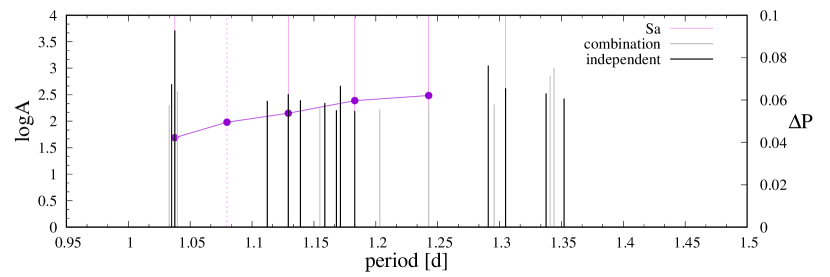
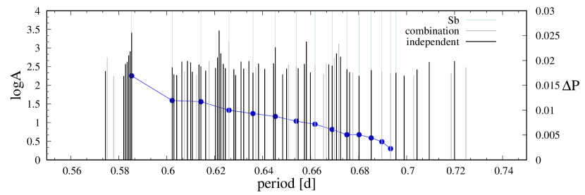
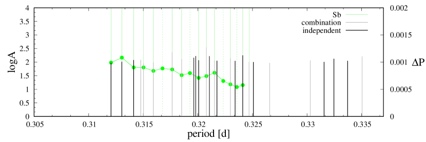
Figure 25: The same as in Fig. 13 but for KIC 9715425.

3.18 KIC 9910544

As KIC 9468611, this star was classified as the SPB variable with frequency grouping and low frequency noise by McNamara et al. (2012).

We found 16 frequency peaks, of which 9 are independent and 2 are combinations. All frequencies have the values below $0.9$ d^-1 and most of them (except 2) concentrate around $0.7$ d^-1. Based on the TDP analysis we concluded that at least the dominant frequency $\nu_{1}=0.723517(7)$ d^-1 is coherent. The other may be incoherent but we are no able to make any reliable conclusion. Due to the small number of frequencies we could not find any regularities in the frequency spectrum for this star.

3.19 KIC 9964614

The star was classified as hybrid $\beta$ Cep/SPB pulsator by Balona et al. (2011); Balona et al. (2015). The authors derived the following atmospheric parameters: $T_{\mathrm{eff}}=20300\,\mathrm{K}$, $\log g=3.9$ (from spectroscopy), $T_{\mathrm{eff}}=19471\,\mathrm{K}$, $\log g=3.75$ (from Strömgren photometry) and $T_{\mathrm{eff}}=23400\pm 7400\,\mathrm{K}$ (from SED fitting).

Our Fourier analysis of the Kepler light curve revealed 246 frequency peaks of which we rejected 41 because of the $2.5\times$Rayleigh limit. From the rest we identified 125 independent frequencies, 76 combinations and 4 harmonics. The highest amplitude signal is very low, $\nu_{1}=0.47356(1)$ d^-1, but independent frequencies are seen up to $\sim 11.4$ d^-1 (see Fig. 9 t). Moreover, the star is located where the SPB and $\beta$ Cep instability strips overlap. Therefore, it is undoubtedly a hybrid pulsator of the SPB/$\beta$ Cep type. The TDP analysis implies that frequencies are coherent, but amplitudes are variable.

For this star there exists a very interesting sequence of frequencies with increasing period spacing. The whole series covers the range from 0.3 d^-1 to 1.7 d^-1 (see Tab. 26 and Fig. 26). However, the two frequencies seem to be missing. The mean period spacing is equal to 0.123 d which corresponds to the frequency difference of 0.064 d^-1. The series can be reproduce with dipole retrograde modes. This star seems to be very promising target for asteroseismic analysis.

Table 15: The same as in Table 13 but for KIC 9964614

ID	$\nu$	$P$	$\Delta P$	$A$	$\frac{\mathrm{S}}{\mathrm{N}}$	fs
	$(\mathrm{d}^{-1})$	$(\mathrm{d})$	$(\mathrm{d})$	$(\mathrm{ppm})$
Sa
$\nu_{9}$	0.31329(3)	3.19198	0.12658	167(2)	9.9	i
$\nu_{6}$	0.32622(2)	3.06540	0.11755	208(2)	12	i
$\nu_{75}$	0.33923(6)	2.94785	0.14161	45(2)	4.1	i
$\nu_{52}$	0.35635(6)	2.80624	0.13046	53(2)	4.5	c
—	0.37372	2.67578	0.15229	—	—	—
$\nu_{48}$	0.39628(5)	2.52349	0.12747	57(2)	4.6	i
$\nu_{74}$	0.41736(6)	2.39602	0.13634	48(2)	4.1	i
—	0.44254	2.25969	0.14803	—	—	—
$\nu_{1}$	0.47356(1)	2.11166	0.14630	503(3)	25	i
$\nu_{8}$	0.50881(2)	1.96536	0.13919	179(2)	11	i
$\nu_{59}$	0.54760(6)	1.82617	0.13451	48(2)	4.5	c
$\nu_{2}$	0.59114(1)	1.69166	0.12249	459(2)	25	i
$\nu_{36}$	0.63728(5)	1.56916	0.14670	69(2)	5.9	c
$\nu_{25}$	0.70301(4)	1.42246	0.12600	89(2)	7.3	i
$\nu_{69}$	0.77133(7)	1.29646	0.14007	40(2)	4.7	c
$\nu_{71}$	0.86476(7)	1.15638	0.11627	38(2)	5.1	i
$\nu_{61}$	0.96144(6)	1.04011	0.08846	46(2)	6.6	c
$\nu_{81}$	1.05081(8)	0.95165	0.08440	33(2)	6.2	i
$\nu_{5}$	1.15307(2)	0.86725	0.10169	231(2)	25	i
$\nu_{99}$	1.3062(1)	0.76556	0.07605	24(2)	5.8	c
$\nu_{84}$	1.45030(8)	0.68951	0.08660	34(2)	8.0	i
$\nu_{86}$	1.65861(8)	0.60292	—	33(2)	8.2	c

Figure 26: The same as in Fig. 23 but for KIC 9964614.

3.20 KIC 10118750

The star was classified as the $\beta$ Cep variable with frequency grouping by McNamara et al. (2012). Kurtz et al. (2015) classified it as the SPB star, whereas Balona et al. (2015) classified it as the SPB/ROT-type variable.

In its light curve we found 111 frequency peaks and rejected 25 because of the $2.5\times$Rayleigh limit. From the rest, we identified 37 independent frequencies, 41 combinations and 8 harmonics. The highest amplitude peak was found in the group around $\sim 3.5$ d^-1. Taking into account the position of the star in the Kiel diagram (Fig. 1) and the high value of $V\sin i$, we concluded that the star is the SPB pulsator. The TDP analysis indicates that at least high amplitude frequencies are coherent.

In the frequency spectrum of KIC 10118750 a clear grouping is visible. The lowest frequency group can be of instrumental origin, but there is a very regular pattern among these peaks that can be associated with dipole retrograde modes. The others hypothetical series are found in the second and third frequency groups (see Tab. 27 and Fig. 27). The mean period differences are 0.01367 d (0.1630 d^-1) for Sa, 0.0030 d (0.1564 d^-1) for Sb and 4.4128 d (0.0062 d^-1) for Sc.

Table 16: The same as in Table 13 but for KIC 10118750

ID	$\nu$	$P$	$\Delta P$	$A$	$\frac{\mathrm{S}}{\mathrm{N}}$	fs
	$(\mathrm{d}^{-1})$	$(\mathrm{d})$	$(\mathrm{d})$	$(\mathrm{ppm})$
Sa
$\nu_{80}$	2.86288(6)	0.34930	0.01893	16(2)	8.0	i
—	3.02694	0.33037	0.01595	—	—	—
$\nu_{64}$	3.18052(5)	0.31441	0.01235	19(2)	9.3	i
$\nu_{6}$	3.310570(4)	0.30206	0.01309	590(2)	83	c
$\nu_{17}$	3.46048(2)	0.28898	0.01351	59(2)	24	c
$\nu_{1}$	3.630231(4)	0.27547	0.01187	1427(4)	67	i
$\nu_{72}$	3.79363(5)	0.26360	0.01043	17(2)	8.3	i
$\nu_{5}$	3.949911(4)	0.25317	0.01319	715(2)	76	c
$\nu_{7}$	4.167051(4)	0.23998	—	540(2)	86	i
Sb
$\nu_{33}$	6.49157(3)	0.15405	0.00347	33(2)	16	i
$\nu_{101}$	6.64094(9)	0.15058	0.00307	10(2)	5.3	i
—	6.77935	0.14751	0.00343	—	—	—
$\nu_{78}$	6.94077(5)	0.14408	0.00305	16(2)	8.1	c
$\nu_{13}$	7.090722(8)	0.14103	0.00330	126(2)	47	i
$\nu_{3}$	7.260475(3)	0.13773	0.00277	1033(2)	85	i
$\nu_{62}$	7.40957(4)	0.13496	0.00304	20(2)	10	c
$\nu_{4}$	7.580143(4)	0.13192	0.00249	802(2)	98	i
—	7.72589	0.12944	0.00284	—	—	—
$\nu_{97}$	7.89907(8)	0.12660	—	11(2)	5.9	c
Sc
$\nu_{58}$	0.01473(4)	67.8996	14.4196	22(2)	5.2	i
$\nu_{39}$	0.01870(3)	53.4800	11.2878	27(2)	6.5	i
$\nu_{51}$	0.02370(4)	42.1922	6.68357	23(2)	5.7	i
$\nu_{20}$	0.02816(2)	35.5086	5.11122	53(2)	9.6	i
$\nu_{40}$	0.03290(3)	30.3974	3.81029	26(2)	6.6	i
$\nu_{36}$	0.03761(3)	26.5871	2.97682	35(2)	6.5	i
—	0.04235	23.6103	2.50001	—	—	—
$\nu_{9}$	0.047370(4)	21.1103	2.72900	385(2)	51	c
$\nu_{18}$	0.05440(2)	18.3813	1.92143	53(2)	11	c
—	0.06075	16.4599	1.77676	—	—	—
$\nu_{79}$	0.06811(5)	14.6831	1.38362	17(2)	4.4	i
$\nu_{65}$	0.07519(5)	13.2995	1.48104	19(2)	4.9	i
$\nu_{81}$	0.08461(6)	11.8185	1.28483	16(2)	4.4	i
$\nu_{84}$	0.09493(5)	10.5336	—	17(2)	4.6	c

Figure 27: The same as in Fig. 13 but for KIC 10118750.

3.21 KIC 10526294

The star was the first time classified as SPB by Debosscher et al. (2011). This was confirmed by McNamara et al. (2012). Then Pápics et al. (2014) found regular period spacing.

In the light curve of KIC 10526294 we found 245 frequency peaks. We rejected 88 of them because of the $2.5\times$Rayleigh limit. We ended up with 78 independent frequencies, 74 combinations and 5 harmonics.

In the frequency spectrum we found one long series of frequencies, Sa (Tab. 28) with nearly constant period differences and slightly increasing frequency differences (see Fig. 28). The mean period difference is 0.0625 d (0.0335 d^-1). This sequence can be reproduce by dipole axisymmetric modes. In general, our series overlaps with those found by Pápics et al. (2014). However, our series contains more frequencies. But we do not find $\nu=0.472220$ d^-1 reported by the cited authors. Other small differences are for frequencies mentioned by Pápics et al. (2014) as do not fulfilling their significance criterion.

Table 17: The same as in Table 13 but for KIC 10526294

ID	$\nu$	$P$	$\Delta P$	$A$	$\frac{\mathrm{S}}{\mathrm{N}}$	fs
	$(\mathrm{d}^{-1})$	$(\mathrm{d})$	$(\mathrm{d})$	$(\mathrm{ppm})$
Sa
$\nu_{174}$	0.39317(7)	2.54344	0.07887	160(8)	4.0	c
$\nu_{81}$	0.40575(5)	2.46458	0.06673	298(8)	5.8	c
—	0.41704	2.39784	0.06077	—	—	—
$\nu_{37}$	0.42789(4)	2.33708	0.07186	533(8)	7.9	i
—	0.44146	2.26522	0.06867	—	—	—
$\nu_{22}$	0.45526(3)	2.19655	0.06698	1160(8)	13	i
$\nu_{144}$	0.46958(7)	2.12957	0.07278	184(8)	4.3	i
$\nu_{151}$	0.48619(7)	2.05680	0.06045	163(8)	4.1	c
$\nu_{51}$	0.50092(5)	1.99635	0.06330	464(8)	7.0	i
$\nu_{142}$	0.51732(7)	1.93305	0.06565	166(8)	4.5	i
$\nu_{16}$	0.53343(2)	1.87470	0.0584	1593(1)	17	i
$\nu_{4}$	0.552610(9)	1.80960	0.06125	8742(8)	49	i
$\nu_{11}$	0.57197(1)	1.74835	0.06375	3384(10)	28	i
$\nu_{59}$	0.59361(5)	1.68460	0.05983	442(8)	7.2	i
$\nu_{18}$	0.61547(2)	1.62477	0.07036	1309(10)	16	i
—	0.64333	1.55441	0.06331	—	—	—
$\nu_{163}$	0.67065(8)	1.49110	0.07000	165(8)	4.1	i
$\nu_{63}$	0.70368(5)	1.42111	0.06002	389(8)	6.8	i
$\nu_{3}$	0.73471(1)	1.36109	0.06644	9461(8)	46	i
$\nu_{97}$	0.77241(6)	1.29465	0.06455	256(8)	5.8	i
$\nu_{5}$	0.81294(1)	1.23010	0.06236	5740(9)	36	i
$\nu_{38}$	0.85636(4)	1.16774	0.05656	514(8)	8.4	i
$\nu_{96}$	0.89995(6)	1.11118	0.06308	267(8)	6.0	c
$\nu_{35}$	0.95412(4)	1.04809	0.06134	599(8)	9.2	i
$\nu_{65}$	1.01343(5)	0.98675	0.05896	416(8)	7.5	i
—	1.07783	0.92779	0.05301	—	—	—
$\nu_{68}$	1.14314(5)	0.87478	0.05188	369(8)	8.8	c
$\nu_{198}$	1.2152(1)	0.82291	0.04768	105(8)	4.5	c
$\nu_{61}$	1.28995(5)	0.77522	0.04289	360(8)	11	c
$\nu_{62}$	1.36550(5)	0.73234	—	363(8)	11	i

Figure 28: The same as in Fig. 23 but for KIC 10526294.

3.22 KIC 10790075

The star was classified as the SPB variable with a low frequency noise by McNamara et al. (2012), whereas, Balona et al. (2015) classified it as a rotational variable with the question mark.

We found in its light curve 43 frequency peaks and rejected 21 because of the $2.5\times$Rayleigh limit. Ultimately, we were left with 11 independent frequencies and 11 combinations. All found frequencies are below $1.1\,\mathrm{d^{-1}}$. The TDP analysis showed that the lowest frequency signal is strongly incoherent (see Fig. 39 in Appendix A). It is hard to state whether we do see incoherent behaviour or an interaction between two close frequencies.

The star lies inside the SPB instability strip but we can say only about a candidate for a coherent SPB-like variability. Therefore we classified the star as a probable SPB pulsator. Since the frequencies varies with time, we did not look for regularities.

3.23 KIC 11293898

The star was classified as a hybrid SPB/$\beta$ Cep pulsator with the frequency grouping by McNamara et al. (2012).

We found 388 frequency peaks and rejected 148 of them because of the $2.5\times$Rayleigh limit. Then, 180 peaks were identified as independent, 52 as combinations and 8 as harmonics. We found 10 groups of frequencies up to $24\,\mathrm{d^{-1}}$. At the end of the Kepler observations there is seen a kind of outburst which is reflected in an amplitude increase. At the same time frequencies seem to be coherent. Despite a presence of high frequencies we identify the star as the SPB pulsator with the frequencies shifted into higher range by the fast rotation. This classification is supported also by the location of the star well inside the SPB instability strip (see Fig. 1).

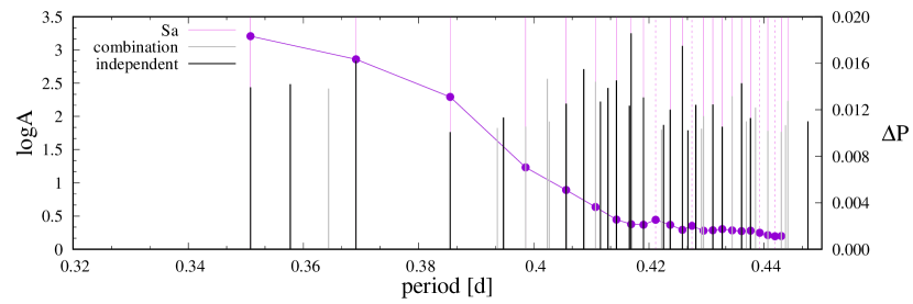
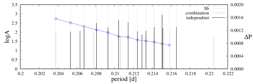
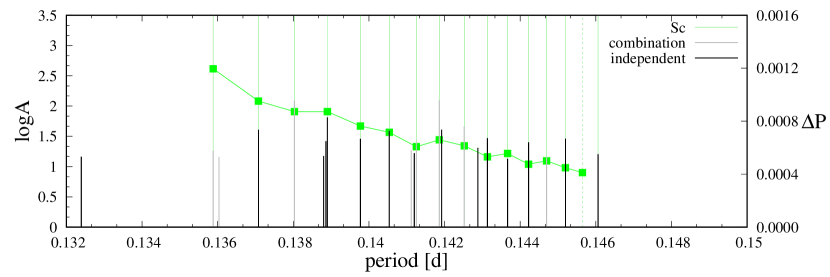
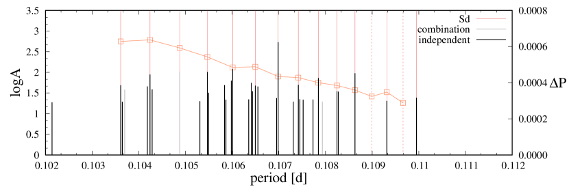
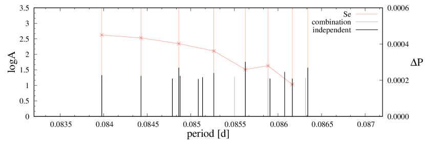
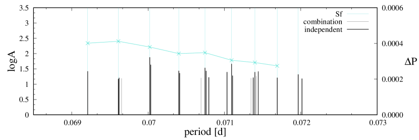
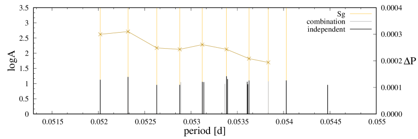
Figure 29: The same as in Fig. 13 but for KIC 11293898.

KIC 11293898 is an example of a star with a very clear frequency grouping. The consecutive groups may be associated with an increasing mode degrees. The lowest frequencies can result from instrumental effects but in the others group we have found seven frequency sequences with decreasing period spacings (see Tab. 18 and Fig. 29). The mean period differences are 0.00406 d (0.02604 d^-1) for Sa, 0.00107 d (0.02416 d^-1) for Sb, 0.00068 d (0.03418 d^-1) for Sc, 0.00045 d (0.03975 d^-1) for Sd, 0.00034 d (0.04657 d^-1) for Se, 0.00035 d (0.06917 d^-1) for Sf and 0.00025 d (0.08930 d^-1) for Sg.

Unstable dipole prograde modes with the mean value of $\Delta P$ well below 0.01 d are predicted by our representative model (see Fig. 12 x). To summarize, the oscillations of KIC 11293898 can be caused by series of consecutive dipole, quadruple and octupole modes. In-depth seismic analysis is necessary to draw more certain conclusions though. This work is already ongoing.

Table 18: The same as in Table 13 but for KIC 11293898

ID	$\nu$	$P$	$\Delta P$	$A$	$\frac{\mathrm{S}}{\mathrm{N}}$	fs
	$(\mathrm{d}^{-1})$	$(\mathrm{d})$	$(\mathrm{d})$	$(\mathrm{ppm})$
Sa
$\nu_{36}$	2.25167(3)	0.44412	0.001136	171(5)	9.1	c
$\nu_{155}$	2.25744(7)	0.44298	0.001114	58(5)	4.0	c
—	2.26313	0.44187	0.001216	—	—	—
$\nu_{145}$	2.26937(6)	0.44065	0.001418	60(5)	4.1	c
—	2.27670	0.43923	0.001598	—	—	—
$\nu_{82}$	2.28501(4)	0.43763	0.001559	94(5)	6.1	i
$\nu_{33}$	2.29318(3)	0.43608	0.001631	313(9)	9.6	i
$\nu_{26}$	2.30179(3)	0.43444	0.001734	201(5)	10	c
$\nu_{121}$	2.31102(6)	0.43271	0.001632	70(5)	4.5	i
$\nu_{48}$	2.31977(3)	0.43108	0.001604	151(5)	7.7	i
$\nu_{76}$	2.32843(4)	0.42947	0.002016	101(5)	6.2	c
—	2.33941	0.42746	0.001670	—	—	—
$\nu_{2}$	2.34859(7)	0.42579	0.002095	1152(8)	43	i
$\nu_{57}$	2.36020(4)	0.42369	0.002538	126(5)	7.2	i
—	2.37442	0.42116	0.002110	—	—	—
$\nu_{28}$	2.38638(3)	0.41905	0.002152	192(5)	9.8	i
$\nu_{1}$	2.398700(6)	0.41689	0.002553	1778(9)	49	i
$\nu_{17}$	2.41348(2)	0.41434	0.003633	348(7)	14	i
$\nu_{16}$	2.43483(2)	0.41071	0.005095	331(5)	14	c
$\nu_{40}$	2.46541(3)	0.40561	0.007039	155(5)	8.3	i
$\nu_{114}$	2.50895(6)	0.39857	0.013100	70(5)	4.6	c
$\nu_{154}$	2.59421(7)	0.38547	0.016338	58(5)	4.1	i
$\nu_{6}$	2.70903(1)	0.36914	0.018324	685(5)	29	i
$\nu_{19}$	2.85054(2)	0.35081	—	274(5)	18	i
Sb
$\nu_{30}$	4.61770(3)	0.21656	0.000739	191(5)	12	i
$\nu_{58}$	4.63352(4)	0.21582	0.000782	123(5)	8.7	c
$\nu_{3}$	4.650365(9)	0.21504	0.000836	882(6)	47	i
$\nu_{34}$	4.66851(3)	0.21420	0.000871	187(5)	11	i
$\nu_{66}$	4.68756(4)	0.21333	0.000903	117(5)	7.6	i
$\nu_{69}$	4.70748(4)	0.21243	0.000987	110(5)	7.3	i
$\nu_{18}$	4.72945(2)	0.21144	0.001009	338(6)	16	i
$\nu_{11}$	4.75212(1)	0.21043	0.001132	449(5)	23	i
$\nu_{32}$	4.77782(3)	0.20930	0.001216	179(5)	10	i
$\nu_{14}$	4.80573(2)	0.20809	0.001321	316(5)	17	i
$\nu_{38}$	4.83643(3)	0.20676	0.001437	164(5)	9.2	i
$\nu_{71}$	4.87027(4)	0.20533	0.001562	106(5)	6.7	i
$\nu_{65}$	4.90760(4)	0.20377	—	110(5)	6.7	c
Sc
$\nu_{313}$	6.8466(2)	0.14606	0.000412	16(5)	4.8	i
—	6.8659	0.14565	0.000449	—	—
$\nu_{210}$	6.8872(1)	0.14520	0.000501	29(5)	7.9	i
$\nu_{333}$	6.9110(3)	0.14470	0.000476	14(5)	4.3	c
$\nu_{237}$	6.9338(2)	0.14422	0.000556	25(5)	6.8	i
$\nu_{336}$	6.9606(3)	0.14367	0.000530	13(5)	4.0	i
$\nu_{234}$	6.9864(2)	0.14314	0.000614	29(5)	6.8	i
$\nu_{174}$	7.01653(8)	0.14252	0.000659	46(5)	11	c
$\nu_{55}$	7.04913(4)	0.14186	0.000607	125(5)	26	c
$\nu_{214}$	7.0794(1)	0.14125	0.000716	25(5)	7.7	c
$\nu_{179}$	7.11550(9)	0.14054	0.000763	39(5)	10	i
$\nu_{221}$	7.1544(1)	0.13978	0.000873	29(5)	7.3	i
$\nu_{133}$	7.19930(6)	0.13890	0.000872	65(5)	15	i
$\nu_{63}$	7.24480(4)	0.13803	0.000951	123(5)	26	c
$\nu_{183}$	7.29509(9)	0.13708	0.001196	41(5)	10	i
$\nu_{283}$	7.3593(2)	0.13588	—	18(5)	5.3	c

Table 18: Continued.

ID	$\nu$	$P$	$\Delta P$	$A$	$\frac{\mathrm{S}}{\mathrm{N}}$	fs
	$(\mathrm{d}^{-1})$	$(\mathrm{d})$	$(\mathrm{d})$	$(\mathrm{ppm})$
Sd
$\nu_{240}$	9.0950(2)	0.10995	0.000288	24(5)	5.2	i
—	9.1189	0.10966	0.000348	—	—	—
$\nu_{265}$	9.1479(2)	0.10931	0.000324	21(5)	4.5	i
—	9.1751	0.10899	0.000359	—	—	—
$\nu_{90}$	9.20543(5)	0.10863	0.000385	95(5)	13	i
$\nu_{205}$	9.2382(1)	0.10825	0.000400	35(5)	6.0	i
$\nu_{194}$	9.2724(1)	0.10785	0.000428	73(9)	6.4	i
$\nu_{175}$	9.30941(8)	0.10742	0.000435	50(5)	7.3	i
$\nu_{8}$	9.34721(1)	0.10698	0.000488	537(5)	59	i
$\nu_{176}$	9.39005(8)	0.10650	0.000485	48(5)	7.2	i
$\nu_{56}$	9.43297(4)	0.10601	0.000543	121(5)	17	i
$\nu_{89}$	9.48152(5)	0.10547	0.000593	102(8)	13	i
$\nu_{147}$	9.5351(1)	0.10488	0.000637	103(8)	8.9	c
$\nu_{99}$	9.59333(5)	0.10424	0.000628	89(5)	12	i
$\nu_{171}$	9.65150(8)	0.10361	—	49(5)	7.7	i
Se
$\nu_{235}$	11.5819(2)	0.08634	0.000177	37(6)	5.7	i
$\nu_{307}$	11.6056(2)	0.08617	0.000280	17(5)	4.0	i
$\nu_{288}$	11.6435(2)	0.08589	0.000259	17(5)	4.3	c
$\nu_{227}$	11.6787(1)	0.08563	0.000362	58(9)	6.0	i
$\nu_{232}$	11.7283(1)	0.08526	0.000402	25(5)	6.0	i
$\nu_{190}$	11.7839(1)	0.08486	0.000434	37(5)	8.6	i
$\nu_{267}$	11.8444(2)	0.08443	0.000450	20(5)	5.0	i
$\nu_{257}$	11.9079(2)	0.08398	—	22(5)	5.4	i
Sf
$\nu_{275}$	13.8955(2)	0.07197	0.000274	21(5)	4.7	i
$\nu_{309}$	13.9486(2)	0.07169	0.000293	16(5)	4.2	i
$\nu_{250}$	14.0058(2)	0.07140	0.000306	25(5)	5.6	i
$\nu_{177}$	14.06600(8)	0.07109	0.000348	46(5)	10	i
$\nu_{201}$	14.1352(1)	0.07075	0.000343	34(5)	8.1	i
$\nu_{223}$	14.2041(1)	0.07040	0.000380	27(5)	7.0	i
$\nu_{196}$	14.2811(1)	0.07002	0.000412	76(10)	8.8	i
$\nu_{327}$	14.3656(3)	0.06961	0.000401	15(5)	4.6	i
$\nu_{228}$	14.4489(1)	0.06921	—	27(5)	7.8	i
Sg
$\nu_{359}$	18.5086(3)	0.05403	0.000194	13(5)	4.6	i
$\nu_{343}$	18.5752(3)	0.05384	0.000208	12(5)	5.0	c
$\nu_{338}$	18.6474(3)	0.05363	0.000243	13(5)	5.3	i
$\nu_{272}$	18.7324(2)	0.05338	0.000261	18(5)	7.9	i
$\nu_{353}$	18.8244(3)	0.05312	0.000243	11(5)	4.8	i
$\nu_{373}$	18.9110(4)	0.05288	0.000248	9(5)	4.2	i
$\nu_{372}$	19.0003(4)	0.05263	0.000310	9(5)	4.3	i
$\nu_{364}$	19.1129(4)	0.05232	0.000300	17(5)	4.8	i
$\nu_{358}$	19.2230(3)	0.05202	—	13(5)	5.3	i

3.24 KIC 11360704

The star was classified as a frequency grouping pulsator by Balona et al. (2011), whereas, McNamara et al. (2012) added the hybrid type of pulsations. Next, Balona et al. (2015) classified it as the SPB/ROT variable. Balona et al. (2011) derived the following atmospheric parameters: $T_{\mathrm{eff}}=20700\,\mathrm{K}$, $\log g=4.1$ (from spectroscopy), $T_{\mathrm{eff}}=17644\,\mathrm{K}$, $\log g=3.89$ (from Strömgren photometry) and $T_{\mathrm{eff}}=18200\pm 5400\,\mathrm{K}$ (from SED fitting).

In its Kepler light curve, one can see a kind of outbursts. We extracted 146 frequency peaks, of which 54 were rejected because of the $2.5\times$Rayleigh limit. We were left with 52 independent frequencies, 36 combinations and 4 harmonics. In the oscillation spectrum we identified frequency grouping with independent frequencies up to $\sim 15\,\mathrm{d}^{-1}$. The star is another fast rotator located inside the SPB instability strip, therefore we classified it as the SPB pulsator. According to the TDP analysis, the frequencies seem to be coherent but their amplitudes are variable.

KIC 11360704 is a very fast rotating star with the minimum rotational velocity of 303 km s^-1. It exhibits characteristic for rapid rotators frequency grouping. There are also three clear regular patterns in its frequency spectrum associated with asymptotic properties of high-order g modes (see Tab .30 and Fig. 30). The Sa series can be associated with dipole retrograde modes. The Sb and Sc sequences seems to be quadrupole axisymmetric and prograde modes, respectively. The mean period differences are 0.7492 d (0.0145 d^-1) for Sa, 0.0072 d (0.0363 d^-1) for Sb and 0.0078 d (0.1516 d^-1) for Sc.

Table 19: The same as in Table 13 but for KIC 11360704

ID	$\nu$	$P$	$\Delta P$	$A$	$\frac{\mathrm{S}}{\mathrm{N}}$	fs
	$(\mathrm{d}^{-1})$	$(\mathrm{d})$	$(\mathrm{d})$	$(\mathrm{ppm})$
Sa
$\nu_{43}$	0.11910(6)	8.39662	0.88955	438(22)	4.4	i
$\nu_{47}$	0.13321(6)	7.50707	0.76234	366(22)	4.2	i
$\nu_{35}$	0.14826(5)	6.74473	0.59570	579(27)	5.0	i
$\nu_{31}$	0.16263(5)	6.14902	—	472(22)	5.3	i
Sb
$\nu_{15}$	2.02780(3)	0.49315	0.00162	870(22)	14	c
—	2.03448	0.49153	0.00213	—	—	—
$\nu_{70}$	2.04333(7)	0.48940	0.00280	574(40)	5.2	i
$\nu_{26}$	2.05509(4)	0.48660	0.00377	782(38)	8.8	i
$\nu_{7}$	2.07115(2)	0.48282	0.00434	1377(23)	21	i
$\nu_{69}$	2.08996(7)	0.47848	0.00460	292(22)	5.2	c
$\nu_{74}$	2.11024(8)	0.47388	0.00791	363(25)	5.0	i
—	2.14603	0.46598	0.00941	—	—	—
$\nu_{39}$	2.19027(5)	0.45657	0.00891	564(32)	7.2	i
$\nu_{95}$	2.23388(9)	0.44765	0.01267	221(21)	4.4	i
—	2.29897	0.43498	0.01419	—	—	—
$\nu_{89}$	2.37648(9)	0.42079	0.01482	231(21)	5.0	i
$\nu_{1}$	2.46321(2)	0.40598	—	2071(22)	35	i
Sc
$\nu_{64}$	3.77265(7)	0.26507	0.00674	308(21)	6.5	c
—	3.87100	0.25833	0.00700	—	—	—
$\nu_{29}$	3.97878(5)	0.25133	0.00734	614(22)	7.4	i
$\nu_{2}$	4.09840(2)	0.24400	0.00793	1703(22)	20	i
$\nu_{37}$	4.23610(5)	0.23607	0.00734	423(21)	5.4	i
$\nu_{4}$	4.37198(2)	0.22873	0.00835	1526(21)	17	i
$\nu_{33}$	4.53751(5)	0.22039	0.00909	487(22)	6.1	c
—	4.73275	0.21129	0.00831	—	—	—
$\nu_{11}$	4.92639(2)	0.20299	0.00832	1092(23)	23	i
$\nu_{103}$	5.1369(1)	0.19467	—	149(22)	5.2	i

Figure 30: The same as in Fig. 13 but for KIC 11360704.

3.25 KIC 11671923

The star was classified as the SPB variable by McNamara et al. (2012); Balona et al. (2015). From its Kepler light curve we derived 38 frequency peaks and rejected 9 because of the $2.5\times$Rayleigh limit. We identified 20 independent frequencies, 8 combinations and 1 harmonic. All frequencies are below $3.3\,\mathrm{d}^{-1}$. Taking into account the observed frequency range and the star’s location in the Kiel diagram (see Fig. 1), we classified the star as the SPB pulsator. Frequencies seem to be coherent apart from the lowest ones $(\sim 0.1\,\mathrm{d^{-1}})$ but the amplitudes are variable.

Since the number of detected frequencies is rather small, we could not find regular patterns.

4 Red noise

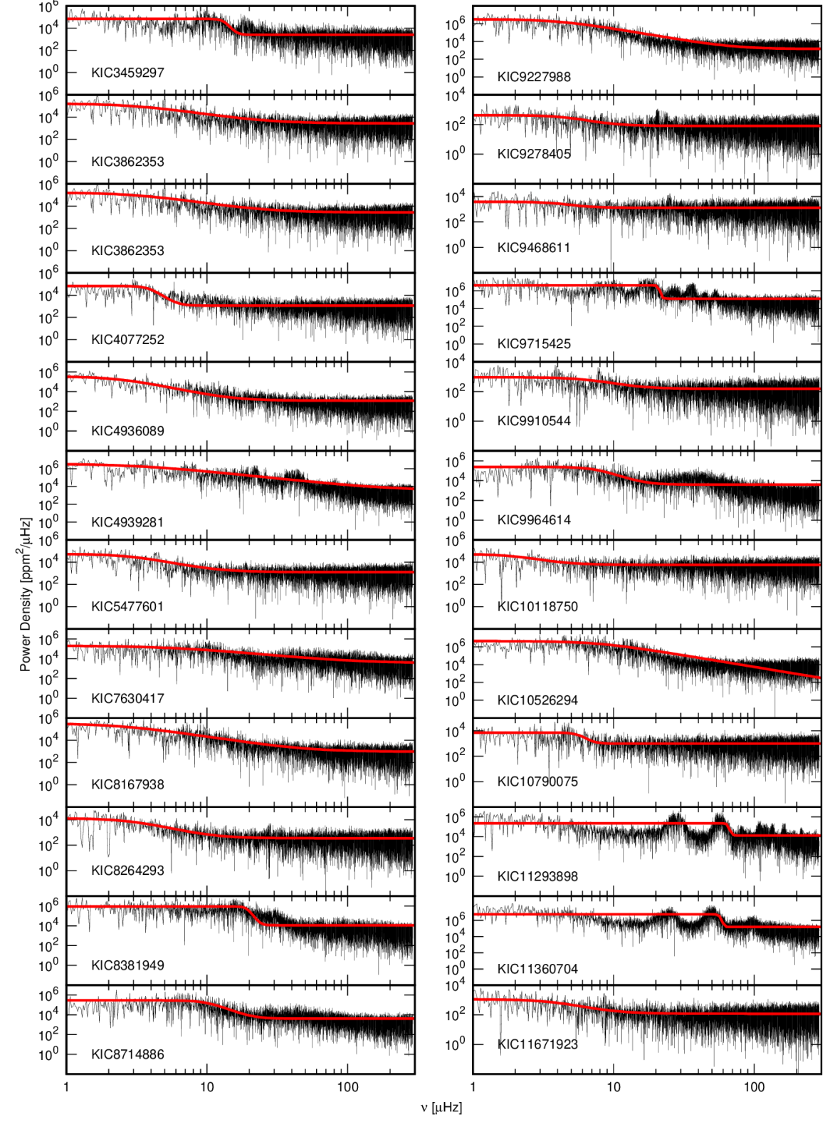
Figure 31: Fourier transforms of the data pre-whitened with all significant frequencies (black lines) and profile from Eq. 5 fitted to these fourier transforms (red lines).

Figure 32: Fitted parameters $a_{0}$, $\nu_{\mathrm{char}}$ and $\gamma$ of profile from Eq. 5. In the top panels are shown relationships between parameters, $\nu_{\mathrm{char}}$, $\alpha_{0}$ and $\gamma$. Effective temperatures are colour coded, whereas point sizes are proportional to the rotation velocities. In the bottom panels the positions of the star on the Kiel diagram are shown with fitted parameters colour coded.

Recently Bowman et al. (2019b) interpreted the so-called red noise in power spectra of a sample of O, B, A and F stars observed by CoRoT as a manifestation of the internal gravity waves (IGW). The authors fitted to the power spectra of their sample stars, the profile in a form:

$$\alpha\left(\nu\right)=\frac{\alpha_{0}}{1+\left(\frac{\nu}{\nu_{\mathrm{char}}}\right)^{\gamma}}+P_{\mathrm{W}}$$ (5)

where $\alpha_{0}$ is a scaling factor, $\gamma$ is the gradient of the linear part of the profile in a log-log graph, $\nu_{\mathrm{char}}$ is the characteristic frequency and $P_{\mathrm{W}}$ is white noise term.

Then Bowman et al. (2019a) and Bowman et al. (2020) studied red noise in a sample of OB stars observed by K2 and TESS missions. Compared to the previous studies the authors found correlations between stochastic phtotometric variability and spectroscopic parameters. However, this is most evident for most massive stars ($M>20\,\mathrm{M}_{\sun}$)

We repeated calculations of Bowman et al. (2019b) and fitted equation 5 to the power spectra of our stars, prewithened with all significant frequencies. Similarly to the cited authors, we used a Markov Chain Monte Carlo procedure. The results are shown in Fig. 31 where fitted profiles are overplotted on the prewithened power spectra. We show 24 stars out of 25 from our sample because in the case of KIC 1430353 our MCMC procedure did not converge at all. Apparently, the considered model is not adequate. Furthermore, the quick inspection of Fig. 31 shows that in the case of KIC 3459297, KIC 4939281, KIC 8381949, KIC 9715425, KIC 9964614, KIC 10526294, KIC 11293898 and KIC 11360704 the adopted model is not correct for the observational data. These results were omitted in the further analysis.

The values of the fitted parameters, $\alpha_{0}$, $\gamma$, $\nu_{\mathrm{char}}$ and $P_{\mathrm{W}}$ for the remaining stars are shown in Fig. 32. In general parameters for our stars are in a good agreement with those found by Bowman et al. (2019b, a, 2020). However, we observe smaller spread in $\nu_{\mathrm{char}}$. Also, we obtained smaller values of this parameter. In addition, for two stars (KIC 4077252 and KIC 10790075) we found relatively high value of $\gamma$ parameter of the order of 10. Such high values seem not to be very common. We also did not find any correlations between parameters from Eq. 5 and stellar parameters such as effective temperature, surface gravity, rotation or luminosity. Since our sample contain stars well below 20 $\mathrm{M}_{\sun}$ this is in line with the findings od Bowman et al. (2020).

Finally, we can use the same arguments as Bowman et al. (2019b, a, 2020) to explain the origin of the observed red noise. First, the values of $\nu_{\mathrm{char}}$ for our stars are below a line for the granulation signal given in Fig. 8 of Bowman et al. (2019b). Since we do not expect granulation for such massive stars, this result is consistent with the standard theory. Second, all our stars have masses approximately below 10 $\mathrm{M}_{\sun}$ so we also do not expect that stellar winds are responsible for the red noise phenomenon. Third, although we are not able to exclude instrumental origin, diversity of red noise profiles (see Fig. 31) may suggest that at least in some stars signal is of astrophysical origin.

Based on our analysis, we can not exclude nor confirm that IGW are the source of the observed red noise. On the one hand, Lecoanet et al. (2019) concluded that low-frequency variability presented by Bowman et al. (2019b) is not due to linearly propagating waves from the core. But on the other hand, the interpretation can be quite different when nonlinear wave propagation is considered as proposed by Ratnasingam et al. (2020). It was recently shown by Horst et al. (2020) that fully compressible nonlinear simulations of waves caused by core convection are in full agreement with the detected red noise features.

5 Conclusions

We analyzed the sample of 25 B-type stars observed during the Kepler mission, for which Hanes et al. (2019) determined stellar parameters. All available observational data were used. The studied stars exhibit rich and complex photometric variability. We detect both coherent as well as incoherent variability. The time scales of these variations are also very diverse. Therefore the origin of the light changes can have a various background, e.g. stellar pulsations, variability in the disk around the star, rotation or binarity.

We would also like to emphasize that distinguishing between combinations and independent frequencies in the dense oscillation spectra is an extremely difficult task.

For many cases more or less regular structures were found. The striking example is KIC 8264293 for which we found clear structure that we associated with prograde dipole modes. In the cases where regular period spacings are not clear, i.e., they are created only from low signal frequencies, one should be careful since they can be of random origin. Therefore, independent mode identification would be invaluable. Another promising test-bed for investigating stellar structure is rare eclipsing binary with SPB-type component, KIC 8167938.

Furthermore, our sample contains stars with different rotational velocities that range from moderate rotators to very fast rotators. On the one hand, this raises a hope for constraints on rotationally induced mixing. Mixing efficiency should increase with rotation rate. Therefore for the fastest rotators it should have the biggest impact on the oscillation spectrum and be easiest to detect. Moreover, successful asteroseismology for enough large sample of stars could allow calibrate mixing efficiency with the rotation speed. And we have prepared a base for detailed seismic analysis of individual stars with oscillation spectra showing certain regularities.

Finally, we detected clear indication of a red noise in the Fourier spectra of our sample stars. In the case of 17 out of 25 stars from our sample it can be manifestation of IGW exicted at the interface between convective core and radiative envelope. But we note that other sources of variability may contribute to the observed red noise as well. However, detailed analysis of this phenomenon and its origin is beyond the scope of this paper.

Data availability

The target pixel files were downloaded from the public data archive at MAST. The lightcurves will be shared on reasonable request to the corresponding author. The full lists of frequencies are available as Supplementary material to this paper.

Appendix A Some extra material

Here we present one quarter cuts of the Kepler light curves for all stars from our set (Fig. 33). In addition there is shown an example of the full light curve with outburst (Fig. 34). Finally, examples of TD periodograms for stars with incoherent signal are plotted in Figs. 35-39.

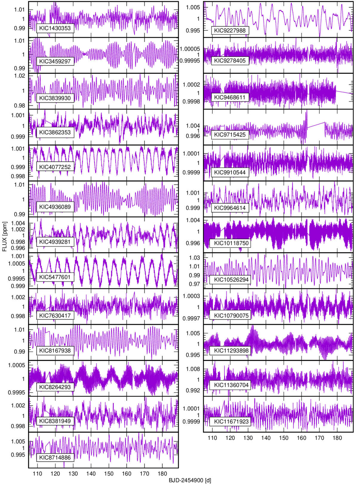
Figure 33: One quarter ($\sim 90$ days) cuts of Kepler light curves for all program stars.

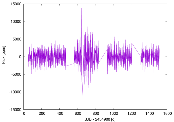
Figure 34: The full Kepler light curve of KIC 4939281.

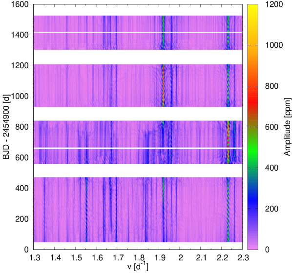
Figure 35: Time dependent periodogram of KIC 4939281.

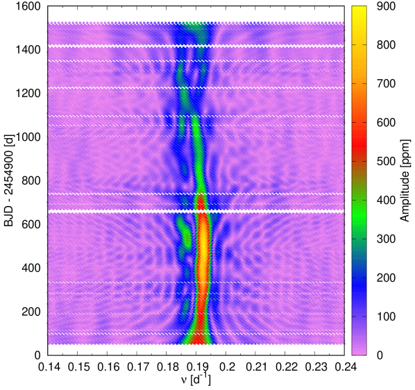
Figure 36: The same as in Fig. 35 but for KIC 5477601.

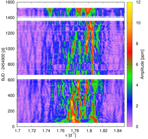
Figure 37: The same as in Fig. 35 but for KIC 9278405.

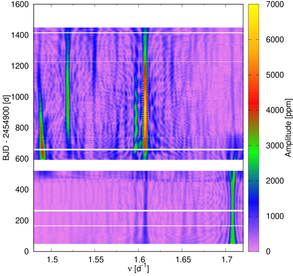
Figure 38: The same as in Fig. 35 but for KIC 9715425.

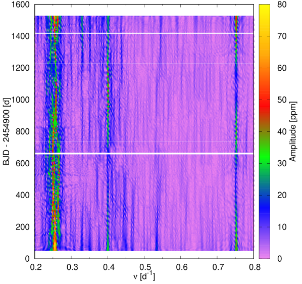
Figure 39: The same as in Fig. 35 but for KIC 10790075.

References

- Angulo et al. (1999) Angulo C., et al., 1999, Nuclear Physics A, 656, 3
- Asplund et al. (2009) Asplund M., Grevesse N., Sauval A. J., Scott P., 2009, ARA&A, 47, 481
- Balona et al. (2011) Balona L. A., et al., 2011, MNRAS, 413, 2403
- Balona et al. (2015) Balona L. A., Baran A. S., Daszyńska-Daszkiewicz J., De Cat P., 2015, MNRAS, 451, 1445
- Balona et al. (2016) Balona L. A., et al., 2016, MNRAS, 460, 1318
- Balona et al. (2019) Balona L. A., et al., 2019, MNRAS, 485, 3457
- Bildsten et al. (1996) Bildsten L., Ushomirsky G., Cutler C., 1996, ApJ, 460, 827
- Bostancı et al. (2015) Bostancı Z. F., et al., 2015, MNRAS, 453, 1095
- Bouabid et al. (2013) Bouabid M. P., Dupret M. A., Salmon S., Montalbán J., Miglio A., Noels A., 2013, MNRAS, 429, 2500
- Bowman et al. (2019a) Bowman D. M., et al., 2019a, Nature Astronomy, 3, 760
- Bowman et al. (2019b) Bowman D. M., et al., 2019b, A&A, 621, A135
- Bowman et al. (2020) Bowman D. M., Burssens S., Simón-Díaz S., Edelmann P. V. F., Rogers T. M., Horst L., Röpke F. K., Aerts C., 2020, A&A, 640, A36
- Breger (1993) Breger M., 1993, in Butler C. J., Elliott I., eds, Vol. 136, IAU Colloq. 136: Stellar Photometry - Current Techniques and Future Developments. p. 106
- Brown et al. (2011) Brown T. M., Latham D. W., Everett M. E., Esquerdo G. A., 2011, AJ, 142, 112
- Buchler & Yueh (1976) Buchler J. R., Yueh W. R., 1976, ApJ, 210, 440
- Cannon & Pickering (1993) Cannon A. J., Pickering E. C., 1993, VizieR Online Data Catalog, p. III/135A
- Cassisi et al. (2007) Cassisi S., Potekhin A. Y., Pietrinferni A., Catelan M., Salaris M., 2007, ApJ, 661, 1094
- Chapellier et al. (2006) Chapellier E., Le Contel D., Le Contel J. M., Mathias P., Valtier J. C., 2006, A&A, 448, 697
- Chapman & Lindzen (1970) Chapman S., Lindzen R., 1970, Atmospheric tides. Thermal and gravitational. Dordrecht: Reidel, 1970
- Chugunov et al. (2007) Chugunov A. I., Dewitt H. E., Yakovlev D. G., 2007, Phys. Rev. D, 76, 025028
- Colgan et al. (2015) Colgan J., Kilcrease D. P., Magee N. H., Abdallah J., Sherrill M. E., Fontes C. J., Hakel P., Zhang H. L., 2015, High Energy Density Physics, 14, 33
- Colgan et al. (2016) Colgan J., et al., 2016, ApJ, 817, 116
- Cox et al. (1992) Cox A. N., Morgan S. M., Rogers F. J., Iglesias C. A., 1992, ApJ, 393, 272
- Cyburt et al. (2010) Cyburt R. H., et al., 2010, ApJS, 189, 240
- Daszyńska-Daszkiewicz et al. (2017a) Daszyńska-Daszkiewicz J., Walczak P., Pamyatnykh A., Jerzykiewicz M., Pigulski A., 2017a, in Second BRITE-Constellation Science Conference: Small satellites—big science. pp 138–144 (arXiv:1701.00961)
- Daszyńska-Daszkiewicz et al. (2017b) Daszyńska-Daszkiewicz J., Pamyatnykh A. A., Walczak P., Colgan J., Fontes C. J., Kilcrease D. P., 2017b, MNRAS, 466, 2284
- Debosscher et al. (2011) Debosscher J., Blomme J., Aerts C., De Ridder J., 2011, A&A, 529, A89
- Dziembowski (1977) Dziembowski W., 1977, Acta Astron., 27, 95
- Dziembowski & Pamiatnykh (1993) Dziembowski W. A., Pamiatnykh A. A., 1993, MNRAS, 262, 204
- Dziembowski et al. (1993) Dziembowski W. A., Moskalik P., Pamyatnykh A. A., 1993, MNRAS, 265, 588
- Dziembowski et al. (2007a) Dziembowski W. A., Daszyńska-Daszkiewicz J., Pamyatnykh A. A., 2007a, Communications in Asteroseismology, 150, 213
- Dziembowski et al. (2007b) Dziembowski W. A., Daszyńska-Daszkiewicz J., Pamyatnykh A. A., 2007b, MNRAS, 374, 248
- Ferguson et al. (2005) Ferguson J. W., Alexander D. R., Allard F., Barman T., Bodnarik J. G., Hauschildt P. H., Heffner-Wong A., Tamanai A., 2005, ApJ, 623, 585
- Frasca et al. (2016) Frasca A., et al., 2016, A&A, 594, A39
- Frinchaboy & Majewski (2008) Frinchaboy P. M., Majewski S. R., 2008, AJ, 136, 118
- Frost (1902) Frost E. B., 1902, ApJ, 15, 340
- Fuller et al. (1985) Fuller G. M., Fowler W. A., Newman M. J., 1985, ApJ, 293, 1
- Gautschy & Saio (1993) Gautschy A., Saio H., 1993, MNRAS, 262, 213
- Guthnick (1913) Guthnick P., 1913, Astronomische Nachrichten, 195, 265
- Handler et al. (2006) Handler G., et al., 2006, MNRAS, 365, 327
- Hanes et al. (2019) Hanes R. J., Waskie S., Labadie-Bartz J. M., Wall A., Boyer A., McSwain M. V., 2019, AJ, 157, 129
- Hardorp et al. (1964) Hardorp J., Theile I., Voigt H. H., 1964, Hamburger Sternw. Warner & Swasey Obs., C03, 0
- Horst et al. (2020) Horst L., Edelmann P. V. F., Andrássy R., Röpke F. K., Bowman D. M., Aerts C., Ratnasingam R. P., 2020, A&A, 641, A18
- Hui-Bon-Hoa & Vauclair (2018) Hui-Bon-Hoa A., Vauclair S., 2018, A&A, 610, L15
- Itoh et al. (1996) Itoh N., Hayashi H., Nishikawa A., Kohyama Y., 1996, ApJS, 102, 411
- Jerzykiewicz et al. (2005) Jerzykiewicz M., Handler G., Shobbrook R. R., Pigulski A., Medupe R., Mokgwetsi T., Tlhagwane P., Rodríguez E., 2005, MNRAS, 360, 619
- Kurtz et al. (2015) Kurtz D. W., Shibahashi H., Murphy S. J., Bedding T. R., Bowman D. M., 2015, MNRAS, 450, 3015
- Kuschnig et al. (1997) Kuschnig R., Weiss W. W., Gruber R., Bely P. Y., Jenkner H., 1997, A&A, 328, 544
- Langanke & Martínez-Pinedo (2000) Langanke K., Martínez-Pinedo G., 2000, Nuclear Physics A, 673, 481
- Lecoanet et al. (2019) Lecoanet D., et al., 2019, ApJ, 886, L15
- Ledoux (1951) Ledoux P., 1951, ApJ, 114, 373
- Lee & Saio (1997) Lee U., Saio H., 1997, ApJ, 491, 839
- Loumos & Deeming (1978) Loumos G. L., Deeming T. J., 1978, Ap&SS, 56, 285
- McNamara et al. (2012) McNamara B. J., Jackiewicz J., McKeever J., 2012, AJ, 143, 101
- Molenda-Żakowicz et al. (2009) Molenda-Żakowicz J., Kopacki G., Steślicki M., Narwid A., 2009, Acta Astron., 59, 193
- Moravveji et al. (2015) Moravveji E., Aerts C., Pápics P. I., Triana S. A., Vandoren B., 2015, A&A, 580, A27
- Moravveji et al. (2016) Moravveji E., Townsend R. H. D., Aerts C., Mathis S., 2016, ApJ, 823, 130
- Moskalik & Dziembowski (1992) Moskalik P., Dziembowski W. A., 1992, A&A, 256, L5
- Nieva & Przybilla (2012) Nieva M. F., Przybilla N., 2012, A&A, 539, A143
- Oda et al. (1994) Oda T., Hino M., Muto K., Takahara M., Sato K., 1994, Atomic Data and Nuclear Data Tables, 56, 231
- Pápics et al. (2014) Pápics P. I., Moravveji E., Aerts C., Tkachenko A., Triana S. A., Bloemen S., Southworth J., 2014, A&A, 570, A8
- Pápics et al. (2015) Pápics P. I., Tkachenko A., Aerts C., Van Reeth T., De Smedt K., Hillen M., Østensen R., Moravveji E., 2015, ApJ, 803, L25
- Pápics et al. (2017) Pápics P. I., et al., 2017, A&A, 598, A74
- Paxton et al. (2011) Paxton B., Bildsten L., Dotter A., Herwig F., Lesaffre P., Timmes F., 2011, ApJS, 192, 3
- Paxton et al. (2013) Paxton B., et al., 2013, ApJS, 208, 4
- Paxton et al. (2015) Paxton B., et al., 2015, ApJS, 220, 15
- Paxton et al. (2018) Paxton B., et al., 2018, ApJS, 234, 34
- Paxton et al. (2019) Paxton B., et al., 2019, ApJS, 243, 10
- Pedersen et al. (2019) Pedersen M. G., et al., 2019, ApJ, 872, L9
- Pinsonneault et al. (2012) Pinsonneault M. H., An D., Molenda-Żakowicz J., Chaplin W. J., Metcalfe T. S., Bruntt H., 2012, ApJS, 199, 30
- Pols et al. (1995) Pols O. R., Tout C. A., Eggleton P. P., Han Z., 1995, MNRAS, 274, 964
- Potekhin & Chabrier (2010) Potekhin A. Y., Chabrier G., 2010, Contributions to Plasma Physics, 50, 82
- Press et al. (2002) Press W. H., Teukolsky S. A., Vetterling W. T., Flannery B. P., 2002, Numerical recipes in C++ : the art of scientific computing
- Ratnasingam et al. (2020) Ratnasingam R. P., Edelmann P. V. F., Rogers T. M., 2020, MNRAS, 497, 4231
- Reed (1998) Reed B. C., 1998, ApJS, 115, 271
- Rogers & Nayfonov (2002) Rogers F. J., Nayfonov A., 2002, ApJ, 576, 1064
- Salmon et al. (2012) Salmon S., Montalbán J., Morel T., Miglio A., Dupret M. A., Noels A., 2012, MNRAS, 422, 3460
- Saumon et al. (1995) Saumon D., Chabrier G., van Horn H. M., 1995, ApJS, 99, 713
- Schwarzenberg-Czerny (1991) Schwarzenberg-Czerny A., 1991, MNRAS, 253, 198
- Slawson et al. (2011) Slawson R. W., et al., 2011, AJ, 142, 160
- Stankov & Handler (2005) Stankov A., Handler G., 2005, ApJS, 158, 193
- Stellingwerf (1978) Stellingwerf R. F., 1978, AJ, 83, 1184
- Still & Barclay (2012) Still M., Barclay T., 2012, PyKE: Reduction and analysis of Kepler Simple Aperture Photometry data, Astrophysics Source Code Library (ascl:1208.004)
- Szewczuk & Daszyńska-Daszkiewicz (2017) Szewczuk W., Daszyńska-Daszkiewicz J., 2017, MNRAS, 469, 13
- Szewczuk & Daszyńska-Daszkiewicz (2018) Szewczuk W., Daszyńska-Daszkiewicz J., 2018, MNRAS, 478, 2243
- Szewczuk et al. (2014) Szewczuk W., Daszyńska-Daszkiewicz J., Dziembowski W., 2014, in Guzik J. A., Chaplin W. J., Handler G., Pigulski A., eds, IAU Symposium Vol. 301, Precision Asteroseismology. pp 109–112 (arXiv:1311.2818), doi:10.1017/S1743921313014178
- Szewczuk et al. (2017) Szewczuk W., Daszyńska-Daszkiewicz J., Walczak P., 2017, in European Physical Journal Web of Conferences. p. 03012 (arXiv:1701.01256), doi:10.1051/epjconf/201716003012
- Tassoul (1980) Tassoul M., 1980, ApJS, 43, 469
- Thompson et al. (2016) Thompson S., Fraquelli D., van Cleve J., Douglas C., 2016, Kepler: A Search for Terrestrial Planets. Kepler Archive Manual.. http://archive.stsci.edu/kepler/manuals/archive_manual.pdf
- Timmes & Swesty (2000) Timmes F. X., Swesty F. D., 2000, ApJS, 126, 501
- Townsend (2003a) Townsend R. H. D., 2003a, MNRAS, 340, 1020
- Townsend (2003b) Townsend R. H. D., 2003b, MNRAS, 343, 125
- Triana et al. (2015) Triana S. A., Moravveji E., Pápics P. I., Aerts C., Kawaler S. D., Christensen-Dalsgaard J., 2015, ApJ, 810, 16
- Unno et al. (1989) Unno W., Osaki Y., Ando H., Saio H., Shibahashi H., 1989, Nonradial oscillations of stars. University of Tokyo Press
- Vinícius et al. (2017) Vinícius Z., Barentsen G., Gully-Santiago M., Cody A. M., Hedges C., Still M., Barclay T., 2017, KeplerGO/PyKE, doi:10.5281/zenodo.835583, https://doi.org/10.5281/zenodo.835583
- Waelkens (1991) Waelkens C., 1991, A&A, 246, 453
- Walczak et al. (2015) Walczak P., Fontes C. J., Colgan J., Kilcrease D. P., Guzik J. A., 2015, A&A, 580, L9
- Walczak et al. (2017a) Walczak P., Daszyńska-Daszkiewicz J., Pamyatnykh A., Handler G., Pigulski A., 2017a, in Zwintz K., Poretti E., eds, Vol. 5, Second BRITE-Constellation Science Conference: Small Satellites - Big Science. pp 173–179 (arXiv:1701.01258)
- Walczak et al. (2017b) Walczak P., Daszyńska-Daszkiewicz J., Pamyatnykh A., 2017b, in European Physical Journal Web of Conferences. p. 06005 (arXiv:1704.06067), doi:10.1051/epjconf/201715206005
- Walczak et al. (2019) Walczak P., et al., 2019, MNRAS, 485, 3544
- Walker et al. (2005) Walker G. A. H., et al., 2005, ApJ, 635, L77
- Zhang et al. (2018) Zhang C., et al., 2018, ApJ, 854, 168