Task-adaptive Neural Process for User Cold-Start Recommendation

Abstract.

User cold-start recommendation is a long-standing challenge for recommender systems due to the fact that only a few interactions of cold-start users can be exploited. Recent studies seek to address this challenge from the perspective of meta learning, and most of them follow a manner of parameter initialization, where the model parameters can be learned by a few steps of gradient updates. While these gradient-based meta-learning models achieve promising performances to some extent, a fundamental problem of them is how to adapt the global knowledge learned from previous tasks for the recommendations of cold-start users more effectively.

In this paper, we develop a novel meta-learning recommender called task-adaptive neural process (TaNP). TaNP is a new member of the neural process family, where making recommendations for each user is associated with a corresponding stochastic process. TaNP directly maps the observed interactions of each user to a predictive distribution, sidestepping some training issues in gradient-based meta-learning models. More importantly, to balance the trade-off between model capacity and adaptation reliability, we introduce a novel task-adaptive mechanism. It enables our model to learn the relevance of different tasks and customize the global knowledge to the task-related decoder parameters for estimating user preferences. We validate TaNP on multiple benchmark datasets in different experimental settings. Empirical results demonstrate that TaNP yields consistent improvements over several state-of-the-art meta-learning recommenders.

1. Introduction

Recommender systems have been successfully applied into a great number of online services for providing precise personalized recommendations (Zhang et al., 2019). Traditional matrix factorization (MF) models and popular deep learning models are among the most widely used techniques, predicting which items a user will be interested in via learning the low-dimensional representations of users and items (Koren et al., 2009; Zheng et al., 2016; He et al., 2017; Liu et al., 2018; Cao* et al., 2021). These models typically work well when adequate user interactions are available, but suffer from cold-start problems. Recommending items to cold-start users who have very sparse interactions, also known as user cold-start recommendation (Bharadhwaj, 2019; Lee et al., 2019; Dong et al., 2020), is one of the major challenges.

To address user cold-start recommendation, early methods (Lops et al., 2011; Bianchi et al., 2017) focus on using side-information, $i.e.$, user profiles and item contents, to infer the preferences of cold-start users. Additionally, many hybrid models integrating side-information into collaborative filtering (CF) are also proposed (Kouki et al., 2015; Wang et al., 2015). For example, collaborative topic regression (Wang and Blei, 2011) combines probabilistic topic modeling (Blei et al., 2003) with MF to enhance model capability of out-of-matrix prediction. However, such informative contents are not always accessible due to the issue of personal privacy (Xin and Jaakkola, 2014), and manually converting them into the useful features of users and items is a non-trivial job (Das et al., 2007).

Inspired by the huge progress on few-shot learning (Snell et al., 2017) and meta learning (Finn et al., 2017), there emerge some promising works (Vartak et al., 2017; Bharadhwaj, 2019; Lee et al., 2019; Du et al., 2019) on solving cold-start problems from the perspective of meta learning, where making recommendations for one user is regarded as a single task (detailed in Definition 3.1). In the training phase, they try to derive the global knowledge across different tasks as a strong generalization prior. When a cold-start user comes in the test phase, the personalized recommendation for her/him can be predicted with only a few interacted items are available, but does so by using the global knowledge already learned.

Most meta-learning recommenders are built upon the well-known framework of model-agnostic meta learning (MAML) (Finn et al., 2017), aiming to learn a parameter initialization where a few steps of gradient updates will lead to good performances on the new tasks. A typical assumption here is the recommendations of different users are highly relevant. However, this assumption does not necessarily hold in actual scenarios. When the users exhibit different purchase intentions, the task relevance among them is actually very weak, which makes it problematic to find a shared parameter initialization optimal for all users. A concrete example is shown in Figure 1: tasks $a$ and $c$ share the transferable knowledge of recommendations, since user $a$ and user $c$ express similar purchase intentions, while task $b$ is largely different from them. Therefore, learning the relevance of different tasks is an important step in adapting the global knowledge for the recommendations of cold-start users more effectively.

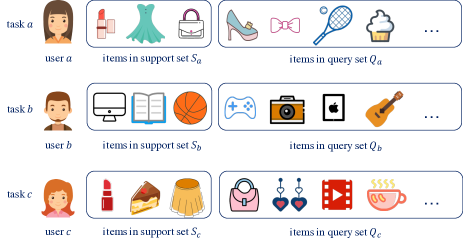
Figure 1. An illustration of the relevance of different tasks. The purchase intentions of user $a$, $b$ and $c$ are manifested by the corresponding user-item interactions. It shows that tasks $a$, $c$ are closely relevant but task $b$ is largely different from them. Each task owns the user-specific support set and query set which will be explained in Definition 3.1.

In this paper, we attempt to establish the connection between user cold-start recommendation and Neural Process (NP) (Garnelo et al., 2018b) to address above problem. NP is a neural-based approximation of stochastic processes. It is also related with meta learning (Garnelo et al., 2018a), since it can directly model the predictive distribution given a conditional prior learned from an arbitrary number of context observations. To be specific, we propose a novel meta-learning framework called task-adaptive neural process (TaNP). Approximating each task as the particular instantiation of a stochastic process, our model is an effective “few-shot function estimator” to characterize the preference of cold-start user. TaNP performs amortized variational inference (Kingma and Welling, 2014) to optimize the model parameters straightforwardly, which can relieve some inherent training issues in above MAML-based recommenders, such as model sensitivity (Antoniou et al., 2019) and being easily stuck into a local optimum (Dong et al., 2020).

On top of that, TaNP includes a novel task-adaptive mechanism that is composed by a customized module and an adaptive decoder. In the customized module, the user interactions in each task are encoded as a deterministic task embedding which is interacted with the global pool to derive a clustering-friendly distribution. By resorting to the learned soft cluster assignments, we can capture the relevance of different tasks holistically. Afterwards, the customized module is combined with different modulation strategies to generate task-related decoder parameters for making personalized recommendations. The main contributions of our work are summarized below:

• This paper proposes a formulation of tackling user cold-start recommendation within the neural process paradigm. Our model quickly learns the predictive distributions of new tasks, and the recommendations of cold-start users can be generated on the fly from the corresponding support set in the test phase.

• The novel introduction of task-adaptive mechanism does not only capture the relevance of different tasks but also incorporates the learned relevance into the modulation of decoder parameters, which is critical to better balance the trade-off between model capacity and adaptation reliability.

• Extensive experiments on benchmark datasets show that our model outperforms several state-of-the-art meta-learning recommenders consistently.

2. Related Work

2.1. Meta Learning

Meta learning covers a wide range of topics and has contributed to a booming study trend. Few-shot learning is one of successful branches of meta learning. We retrospect some representative meta-learning models with strong connections to our work. They can be divided into the following common types. 1) Memory-based approaches (Santoro et al., [n.d.]; Kaiser et al., 2017): combining deep neural networks (DNNs) with the memory mechanism to enhance the capability of storing and querying meta-knowledge. 2) Optimization-based approaches (Ravi and Larochelle, 2017; Li et al., 2017): a meta-learner, e.g. recurrent neural networks (RNNs) is trained to optimize target models. 3) Metric-based approaches (Vinyals et al., 2016; Snell et al., 2017): learning an effective similarity metric between new examples and other examples in the training set. 4) Gradient-based approaches (Finn et al., 2017; Nichol and Schulman, 2018): learning an shared initialization where the model parameters can be trained via a few gradient updates on new tasks. Most meta-learning models follow an episodic learning manner. Among them, MAML is one of the most popular frameworks, which falls into the fourth type. Some MAML-based works (Vuorio et al., 2019; Yao et al., 2019) consider that the sequence of tasks may originate from different task distributions, and try various task-specific adaptations to improve model capability.

2.2. User Cold-Start Recommendation

CF-based methods have been revolutionizing recommender systems in recent years due to the effectiveness of learning low-dimensional embeddings, like matrix factorization (Gu et al., 2010; He et al., 2016) and deep learning (He et al., 2017; Ma et al., 2019). However, most of them are not explicitly tailored for solving user cold-start recommendation, e.g., new registered users only have very few interactions (Park and Chu, 2009). Previous methods (Bianchi et al., 2017; Gao et al., 2018) mainly try to incorporate side-information into CF for alleviating this problem.

Inspired by the significant improvements of meta learning, the pioneering work (Vartak et al., 2017) provides a meta-learning strategy to solve cold-start problems. It uses a task-dependent way to generate the varying biases of decision layers for different tasks, but it is prone to underfitting and is not flexible enough to handle various recommendation scenarios (Bharadhwaj, 2019). MeLU (Lee et al., 2019) adopts the framework of MAML. Specifically, it divides the model parameters into two groups, i.e., the personalized parameter and the embedding parameter. The personalized parameter is characterized as a fully-connected DNN to estimate user preferences. The embedding parameter is referred as the embeddings of users and items learned from side-information. An inner-outer loop is used to update these two groups of parameters. In the inner loop, the personalized parameter is locally updated via the prediction loss of support set in current task. In the outer loop, these parameters are globally updated according to the prediction loss of query sets in multiple tasks. Through the fashion of local-global update, MeLU can provide a shared initialization for different tasks.

The later work MetaCS (Bharadhwaj, 2019) is much similar to MeLU, and the main difference is that the local-global update involves all parameters from input embedding to model prediction. To generalize well for different tasks, two most recent works MetaHIN (Lu et al., 2020) and MAMO (Dong et al., 2020) propose different task-specific adaptation strategies. In particular, MetaHIN incorporates heterogeneous information networks (HINs) into MAML to capture rich semantics of meta-paths. MAMO introduces two memory matrices based on user profiles: a feature-specific memory that provides a specific bias term for the shared parameter initialization; a task-specific memory that guides the model for predictions. However, these two gradient-based meta-learning models may still suffer from potential training issues in MAML, and the model-level innovations of them are closely related with side-information, which limits their application scenarios.

2.3. Neural Process

NP is a neural-based formulation of stochastic processes that model the distribution over functions (Garnelo et al., 2018b, a). It is a class of neural latent variable model that combines the strengths of Gaussian Process (GP) and DNNs to achieve flexible function approximations. NP mainly concentrates on the domains of low-dimensional function regression and uncertainty estimation (Louizos et al., 2019). Meanwhile, there have been a growing number of researches on improving the expressiveness of vanilla NP model. For example, ANP (Kim et al., 2019) introduces a self-attention NP to alleviate the underfitting of NP; CONVCNP (Gordon et al., [n.d.]) models the translation equivariance in data and extends task representations into function space. NP is also suitable to meta-learning problems (Requeima et al., 2019), because it provides an effective way to model the predictive distribution conditioned on a permutation-invariant representation learned from context observations. Our model is the first study that leverages the principle of NP to solve user cold-start recommendation, involving learn the discrete user-item relational data which is largely different from previous works. Moreover, TaNP includes a novel task-adaptive mechanism to better balance the trade-off between model capacity and adaptation reliability.

Table 1. Notations

Notation	Description
$U$ and $V$	user set and item set
$U^{tr}$ and $U^{te}$	training user set and test user set
$\mathcal{T}^{tr}$ and $\mathcal{T}^{te}$	training task set and test task set
$\tau_{i}$, $S_{i}$ and $Q_{i}$	task $i$, support set $i$ and query set $i$
$x_{i,j}=(u_{i},v_{j})$	an interaction between $u_{i}$ and $v_{j}$
$y_{i,j}$	the actual rating of $x_{i,j}$
$N_{i}$	the number of interactions in $\tau_{i}$
$N_{S_{i}}$ and $N_{Q_{i}}$	the numbers of interactions in $S_{i}$ and $Q_{i}$
$\bm{c}_{i,n}$	the one-hot content vector of $u_{i}$
$\bm{E}_{n}$	the shared matrix in embedding layers
$h_{\theta}$	shared encoder for all tasks
$m_{\phi}$	task identity network
$\bm{A}$	global pool
$\bm{C}$	soft cluster assignment matrix
$\bm{D}$	clustering target distribution
$g_{\omega_{i}}$	adaptive decoder for $\tau_{i}$
$\bm{\gamma}^{l}_{i}$, $\bm{\beta}^{l}_{i}$, $\bm{\eta}^{l}_{i}$ and $\bm{\delta}^{l}_{i}$	feature modulation parameters of $g_{\omega_{i}}$ for the $l$-th layer

3. Preliminaries

We formulate the problem of user cold-start recommendation from the meta-learning perspective. Following the traditional episodic learning manner, we first give the formal definition of task (episode).

Definition 3.1.

(TASK) Given the user set $U$, the item set $V$ and a specific user $u_{i}\in U$, making the personalized recommendation for $u_{i}$ is defined as a task $\tau_{i}$. $\tau_{i}$ includes the available interactions of $u_{i}$, i.e., $\{x_{i,j},y_{i,j}\}_{j=1}^{N_{i}}$. $x_{i,j}$ denotes a tuple $(u_{i},v_{j})$ in which $v_{j}\in V$ denotes an item and $y_{i,j}$ is $u_{i}$’s actual rating of item $v_{j}$. $N_{i}$ denotes the number of interactions in $\tau_{i}$. For notation simplicity, we also denote $\tau_{i}=\{x_{i,j},y_{i,j}\}_{j=1}^{N_{i}}$. $\tau_{i}$ contains few interactions as the support set $S_{i}$ and remaining interactions as query set $Q_{i}$, i.e., $\{x_{i,j},y_{i,j}\}_{j=1}^{N_{i}}=S_{i}\cup Q_{i}$. Here we denote $S_{i}=\{x_{i,j},y_{i,j}\}^{N_{S_{i}}}_{j=1}$ and $Q_{i}=\{x_{i,j},y_{i,j}\}^{N_{S_{i}}+N_{Q_{i}}}_{j=N_{S_{i}}+1}$. $N_{S_{i}}$ denotes the number of interactions in $S_{i}$, which is typically set with a small value, and $N_{Q_{i}}$ is the number of interactions in $Q_{i}$ with $N_{S_{i}}+N_{Q_{i}}=N_{i}$.

Note a meta-learning recommender is first learned on each support set (learning procedure) and is then updated according to the prediction loss over multiple query sets (learning-to-learn procedure). Through the guide of the second procedure in many iterations, this meta-learning model can derive the global knowledge across different tasks and adapts such knowledge well for a new task $\tau_{i}$ with only $S_{i}$ available.

For this purpose, we split $U$ into two disjoint sets: training user set $U^{tr}$ and test (cold-start) user set $U^{te}$. The set of all training tasks is denoted as $\mathcal{T}^{tr}=\{\tau_{i}|u_{i}\in U^{tr}\}$ and the set of all test tasks is denoted as $\mathcal{T}^{te}=\{\tau_{i}|u_{i}\in U^{te}\}$. In the training phase, we can train our model following a learning-to-learn manner for each training task. In the test phase, when a cold-start user $u_{i^{\prime}}\in U^{te}$ comes, our goal is to find which items $u_{i^{\prime}}$ will be interested in, based on a small number of interactions in $S_{i^{\prime}}$ and the global knowledge learned from $\mathcal{T}^{tr}$. The notations used in this paper are summarized in Table 1. In addition, according to the concrete value of $y_{i,j}$, the personalized recommendation can be either viewed as a binary classification to indicate whether $u_{i}$ engages with $v_{j}$, or a regression problem that $v_{j}$ has different ratings that need to be assessed by $u_{i}$.

4. Task-adaptive Neural Process

In this section, we first describe how to handle user cold recommendation from the view of NP. Then we analysis the potential issue of it and propose an effective solution, i.e., the task-adaptive mechanism. Our model includes three parts: encoder, customization module and adaptive decoder. The encoder is used to obtain the variational prior and posterior via a lower bound estimation. The customization module is used to recognize the task identity and to learn the relevance of different tasks. It is further coupled with different modulation strategies to generate the model parameters of adaptive decoder. In addition, our model includes different embedding strategies and prediction losses, which can be applicable to different recommendation scenarios.

4.1. Overview

In our model, we assume each task $\tau_{i}=\{x_{i,j},y_{i,j}\}_{j=1}^{N_{i}}$ is associated with an instantiation of stochastic process $f_{i}$ from which the observed interactions of user $u_{i}$ are drawn. The corresponding joint distribution $\rho$ can be given as:

(1) $$\begin{split}\rho_{x_{i,1:N_{i}}}(y_{i,1:N_{i}})=\int p(f_{i})p(y_{i,1:N_{i}}|f_{i},x_{i,1:N_{i}})df_{i}\end{split}$$

Here we use $x_{i,1:N_{i}}$ and $y_{i,1:N_{i}}$ to denote $\{x_{i,j}\}_{j=1}^{N_{i}}$ and $\{y_{i,j}\}_{j=1}^{N_{i}}$ decoupled from $\tau_{i}$. Motivated by NP, we can approximate the above stochastic process via a fixed-dimensional vector $\bm{z}_{i}$ and the learnable non-linear functions parameterized by DNNs. The complete generation process with the i.i.d. condition can be given as follows,

(2) $$\begin{split}p(y_{i,1:N_{i}}|x_{i,1:N_{i}})=\int p(\bm{z}_{i})\prod_{j=1}^{N_{i}}p(y_{i,j}|x_{i,j},\bm{z}_{i})d\bm{z}_{i}.\end{split}$$

In such a way, sampling $\bm{z}_{i}$ from $p(\bm{z}_{i})$ can be viewed as a concrete function realization.

Since the true posterior is intractable, we use amortized variational inference (Mnih and Gregor, 2014) to learn it. The variational posterior of the latent variable $\bm{z}_{i}$ is defined as $q(\bm{z}_{i}|\tau_{i})$, and we have the following evidence lower-bound (ELBO) objective with step-by-step derivations:

(3) $$\begin{split}&{\rm log}p(y_{i,1:N_{i}}|x_{i,1:N_{i}})={\rm log}\int p(\bm{z}_{i},y_{i,1:N_{i}}|x_{i,1:N_{i}})d\bm{z}_{i}\\ &={\rm log}\int p(\bm{z}_{i},y_{i,1:N_{i}}|x_{i,1:N_{i}})\frac{q(\bm{z}_{i}|\tau_{i})}{q(\bm{z}_{i}|\tau_{i})}d\bm{z}_{i}\\ &\geq\mathbb{E}_{q(\bm{z}_{i}|\tau_{i})}\big{[}{\rm log}\frac{p(\bm{z}_{i},y_{i,1:N_{i}}|x_{i,1:N_{i}})}{q(\bm{z}_{i}|\tau_{i})}\big{]}\\ &=\mathbb{E}_{q(\bm{z}_{i}|\tau_{i})}\big{[}{\rm log}\frac{p(\bm{z}_{i})p(y_{i,1:N_{i}}|x_{i,1:N_{i}},\bm{z}_{i})}{q(\bm{z}_{i}|\tau_{i})}\big{]}\\ &=\mathbb{E}_{q(\bm{z}_{i}|\tau_{i})}\big{[}\sum_{j=1}^{N_{i}}{\rm log}p(y_{i,j}|x_{i,j},\bm{z}_{i})+{\rm log}\frac{p(\bm{z}_{i})}{q(\bm{z}_{i}|\tau_{i})}\big{]}.\end{split}$$

Each $\tau_{i}$ is constituted by $S_{i}$ and $Q_{i}$, and we should pay more attention to make predictions for $Q_{i}$ given $S_{i}$. Therefore, Eq.(3) is alternatively defined as:

(4) $$\begin{split}&{\rm log}p(y_{i,1:N_{Q_{i}}}|x_{i,1:N_{Q_{i}}},S_{i})\\ &\geq\mathbb{E}_{q(\bm{z}_{i}|\tau_{i})}\big{[}\sum_{j=1}^{N_{Q_{i}}}{\rm log}p(y_{i,j}|x_{i,j},\bm{z}_{i})+{\rm log}\frac{q(\bm{z}_{i}|S_{i})}{q(\bm{z}_{i}|\tau_{i})}\big{]}.\end{split}$$

We use the variational prior $q(\bm{z}_{i}|S_{i})$ to approximate $p(\bm{z}_{i}|S_{i})$ in Eq.(4), since $p(\bm{z}_{i}|S_{i})$ is also intractable. Such an approximation can be considered as a regularization term of KL divergence to approximate the consistency condition of stochastic process (Oksendal, 2013). Furthermore, to model the distribution over random functions, we add the variability of interaction sequence to $\tau_{i}$ as suggested in (Garnelo et al., 2018b). Then, each sample of $\bm{z}_{i}$ is regarded as a realisation of the corresponding stochastic process.

From above formulations, our model can be extended to learn multiple tasks with different stochastic processes in a meta-learning framework. However, both the encoder $q(\bm{z}|\tau)$/$q(\bm{z}|S)$ and the decoder $p(y|\bm{z},x)$ are the global parameters that are shared by all training tasks $\mathcal{T}^{tr}$, and the relevance of different tasks has been ignored. Hence, the above framework is inflexible to adjust model capacity for different tasks. In other words, it may lead to underfitting for some relative complex tasks, and suffers from overfitting for some easy tasks. To better balance the trade-off between model capacity and adaptation reliability, we introduce a novel task-adaptive mechanism. The overall training framework of our model is shown in Figure 2.

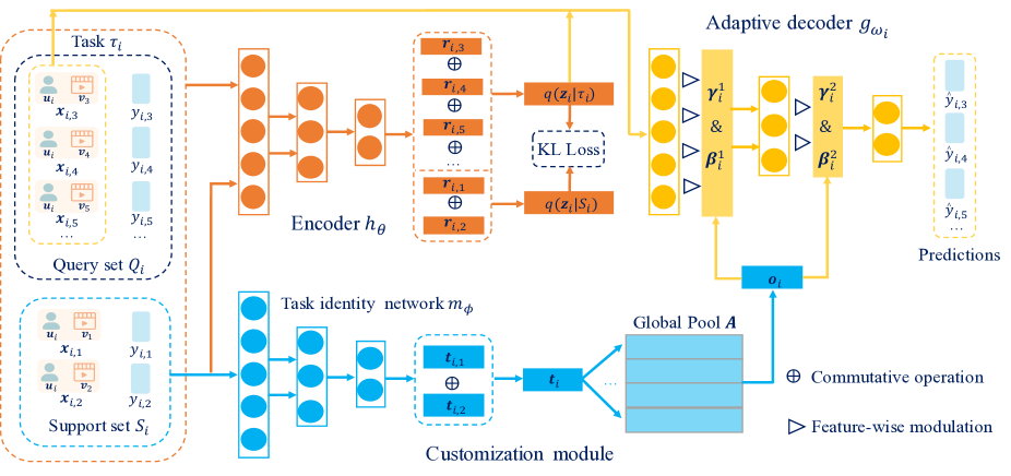
Figure 2. The framework of TaNP in the training phase. TaNP includes the encoder $h_{\theta}$, the customization module (task identity network $m_{\phi}$ and global pool $\bm{A}$) and the adaptive decoder $g_{\omega_{i}}$. Both of $S_{i}$ and $\tau_{i}$ are encoded by $h_{\theta}$ to generate the variational prior and posterior, respectively. The final task embedding $\bm{o}_{i}$ learned from the customized module is used to modulate the model parameters of $g_{\omega_{i}}$. $\bm{z}_{i}$ sampled from $q(\bm{z}_{i}|\tau_{i})$ is concatenated with $\bm{x}_{i,j}$ to predict $\hat{y}_{i,j}$ via $g_{\omega_{i}}$.

4.2. Embedding Layers

We first use the embedding layers to generate initial user and item embeddings as the inputs of TaNP. Our model is compatible with side-information of users and items, thus we provide two embedding strategies. Taking a user $u_{i}$ for example, when categorical contents of $u_{i}$ are available, we would generate a content embedding for each categorical content and concatenate them together to obtain the initial user embedding. Given $n$ user contents, the embedding procedure is defined as:

(5) $$\begin{split}\bm{u}_{i}=\big{[}\bm{E}_{1}\bm{c}_{i,1}|...|\bm{E}_{n}\bm{c}_{i,n}\big{]},\end{split}$$

where $[\cdot|\cdot]$ is the concatenation operation, $\bm{c}_{i,n}$ is the one-hot vector of $n$-th categorical content of $u_{i}$, and $\bm{E}_{n}$ represents the corresponding shared embedding matrix. When such kind of user contents are not available, the user embedding can be obtained by

(6) $$\begin{split}\bm{u}_{i}=\sigma(\bm{W}_{2}\sigma(\bm{W}_{1}\bm{e}_{i}+\bm{b}_{1})+\bm{b}_{2}),\end{split}$$

where $\{\bm{W}_{1},\bm{W}_{2}\}$ denotes weight matrices, $\{\bm{b}_{1},\bm{b}_{2}\}$ denotes bias vectors, $\sigma$ is the sigmoid activation function, and $\bm{e}_{i}$ is the one-hot vector of $u_{i}$. Notice that the initial item embeddings are obtained by following the similar embedding process.

4.3. Encoder

Given $S_{i}$ and $\tau_{i}$, our encoder tries to generate the variational approximations $q(\bm{z}_{i}|S_{i})$ and $q(\bm{z}_{i}|\tau_{i})$ respectively. Concretely, for an interaction $(x_{i,j},y_{i,j})$ in $S_{i}$ or $\tau_{i}$ , the encoder $h_{\theta}$ would produce a corresponding embedding $\bm{r}_{i,j}$ via the following operation:

(7) $$\begin{split}\bm{r}_{i,j}=h^{l}(h^{l-1}(\cdot\cdot\cdot h^{1}([\bm{u}_{i}|\bm{v}_{j}|y_{i,j}]))),\end{split}$$

where $h(\bm{x})={\rm ReLU}(\bm{Wx}+\bm{b})$ is a fully-connected layer with the corresponding $\bm{W}$ and $\bm{b}$, and $l$ is the number of stacked layers. Given a set of observed interactions, the encoder would then aggregate these encoded vectors to generate a permutation-invariant representation $\bm{r}_{i}$. For example, to model $q(\bm{z}_{i}|\tau_{i})$, we have

(8) $$\begin{split}\bm{r}_{i}=\bm{r}_{i,1}\oplus\bm{r}_{i,2}\oplus\ ...\ \bm{r}_{i,N_{i-1}}\oplus\bm{r}_{i,N_{i}},\end{split}$$

where $\oplus$ is a commutative operation and we use a mean operation, i.e., $\bm{r}_{i}=\frac{1}{N_{i}}\sum_{j=1}^{N_{i}}\bm{r}_{i,j}$ for efficiency. This permutation invariance in Eq.(8) is also an important step to approximate the exchangeability condition of stochastic process (Oksendal, 2013). The reparameterization trick (Kingma and Welling, 2014) is adopted to express the random variable, i.e., $\bm{z}_{i}\thicksim\mathcal{N}(\bm{\mu}_{i},{\rm diag}(\bm{\sigma}_{i}^{2}))$. It can be formally defined as:

(9) $$\begin{split}\bm{r}_{i}=~{}&{\rm ReLU}(\bm{W}_{s}\bm{r}_{i}),\\ \bm{\mu}_{i}=\bm{W}_{\mu}&\bm{r}_{i},\ {\rm log}\bm{\sigma}_{i}=\bm{W}_{\sigma}\bm{r}_{i},\\ \bm{z}_{i}=\bm{\mu}_{i}+&\bm{\epsilon}\odot\bm{\sigma}_{i},\ \bm{\epsilon}\thicksim\mathcal{N}(\bm{0},\bm{I}),\end{split}$$

where $\odot$ denotes the element-wise product, $\bm{\epsilon}$ is the Gaussian noise, and $\{\bm{W}_{s},\bm{W}_{\mu},\bm{W}_{\sigma}\}$ are weight matrices.

4.4. Customization Module

The customization module seeks to learn the relevance of different tasks. It contains a task identity network $m_{\phi}$ and a global pool $\bm{A}$. $m_{\phi}$ is used to produce a temporary task embedding $\bm{t}_{i}$ from the corresponding support set $S_{i}$. Formally, it encodes each interaction $(x_{i,j},y_{i,j})$ in $S_{i}$ as a low-dimensional representation $\bm{t}_{i,j}$, which can be described as:

(10) $$\begin{split}\bm{t}_{i,j}=m^{l}(m^{l-1}(\cdot\cdot\cdot m^{1}([\bm{u}_{i}|\bm{v}_{j}|y_{i,j}]))).\end{split}$$

$m_{\phi}$ keeps the same network structure with Eq.(7). $\{\bm{t}_{i,j}\}_{j=1}^{N_{S_{i}}}$ is aggregated into $\bm{t}_{i}$ via the same operation in Eq.(8). The global pool $\bm{A}=[\bm{a}_{1},...,\bm{a}_{k}]\in R^{d\times k}$ is a differentiable external resource that preserves the soft c ter centroids. Each $\bm{t}_{i}$ would interact with $\bm{A}$ to derive soft cluster assignments ($k$ is a hyper-parameter that represents the number of soft cluster centroids). We use the Student’s t-distribution as a kernel to measure the normalized similarity between $\bm{t}_{i}$ and $\bm{a}_{j}$ as follows,

(11) $$\begin{split}c_{i,j}=\frac{(1+||\bm{t}_{i}-\bm{a}_{j}||^{2}/\alpha)^{-\frac{\alpha+1}{2}}}{\sum_{j^{\prime}}(1+||\bm{t}_{i}-\bm{a}_{j^{\prime}}||^{2}/\alpha)^{-\frac{\alpha+1}{2}}},\end{split}$$

where $\alpha$ is the degree of freedom of the Student’s t-distribution. The final task embedding $\bm{o}_{i}$ is generated by the following operation:

(12) $$\begin{split}\bm{o}_{i}=\sigma(\bm{W}_{o}(\bm{t}_{i}+\bm{A}\bm{c}_{i}^{T})),\end{split}$$

where $\bm{W}_{o}$ is a weight matrix. In fact, the sequence of interactions in each task represents the purchase intentions of a specific user, and different users may have similar or diverse intentions. $\bm{A}$ includes multiple high-level features that are related with user intentions, which is similar to the intention prototypical embeddings used in disentangled recommendation models (Ma et al., 2019, 2020). Each task has access to $\bm{A}$, and the correlation degree is reflected by $\bm{c}_{i}$. Therefore, the relevance of different tasks can be globally learned, which is further incorporated into the final task embedding through the Eq.(12).

The normalized assignments of all training tasks construct a assignment matrix $\bm{C}=[\bm{c}_{1},...,\bm{c}_{|\mathcal{T}^{tr}|}]\in R^{|\mathcal{T}^{tr}|\times k}$. As suggested by (Xie et al., 2016), we use an unsupervised clustering loss $\mathcal{L}_{u}$ with the guidance of an auxiliary clustering target distribution $\bm{D}$. $\mathcal{L}_{u}$ is defined as a KL divergence loss between $\bm{C}$ and $\bm{D}$:

(13) $$\begin{split}\mathcal{L}_{u}={\rm KL}(\bm{D}||\bm{C})=\sum_{i}\sum_{j}\bm{D}_{i,j}{\rm log}\frac{\bm{D}_{i,j}}{\bm{C}_{i,j}}.\end{split}$$

where the clustering target distribution $\bm{D}$ can be defined as follows,

(14) $$\begin{split}\bm{D}_{i,j}=\frac{(\bm{C}_{i,j})^{2}/\sum_{i}\bm{C}_{i,j}}{\sum_{j^{\prime}}(\bm{C}_{i,j^{\prime}})^{2}/\sum_{i}\bm{C}_{i,j^{\prime}}}.\end{split}$$

Our clustering improves cluster purity and puts more emphasis on tasks assigned with high confidence.

4.5. Adaptive Decoder

The original decoder $g_{\omega}$ in Eq.(4) is used to learn the conditional likelihood $p(y|x,z)$, which is a global predictor shared by all tasks. In this section, TaNP introduces an adaptive decoder $g_{\omega_{i}}$ in a parameter-efficient manner. We describe two candidate modulation strategies to generate the model parameters of adaptive decoder via using the final task embedding $\bm{o}_{i}$. The first variant is Feature-wise Linear Modulation (FiLM) (Perez et al., 2018). Based on this basic modulation, we propose the second modulation strategy, i.e., Gating-FiLM.

4.5.1. FiLM

FiLM tires to adaptively influence the prediction of a DNN by applying a feature-wise affine transformation on its intermediate features. It has been proved to be highly effective in many domains (Cadene et al., 2019; Brockschmidt, 2020). Here we employ FiLM to scale and shift the feature of each layer of our decoder via two generated parameters. The adaptation of $g_{\omega_{i}}$ for the $l$-th layer can be defined as:

(15) $$\begin{split}\bm{\gamma}^{l}_{i}={\rm tanh}(\bm{W}_{\gamma}^{l}\bm{o}_{i}),\quad&\bm{\beta}^{l}_{i}={\rm tanh}(\bm{W}_{\beta}^{l}\bm{o}_{i}),\\ \bm{g}_{i,j}^{l+1}={\rm ReLU}(\bm{\gamma}^{l}_{i}\odot(&\bm{W}_{\omega}^{l}\bm{g}_{i,j}^{l}+\bm{b}_{\omega}^{l})+\bm{\beta}^{l}_{i}),\end{split}$$

where $\{\bm{W}_{\gamma}^{l},\bm{W}_{\beta}^{l},\bm{W}_{\omega}^{l}\}$ denotes layer-wise weight matrices, $\bm{b}_{\omega}^{l}$ denotes a bias vector, and $\bm{g}_{i,j}^{l}$ is the input of $l$-th layer of our decoder. The non-linearity function $\rm tanh$ is applied here to restrict the output of modulation to be in $[-1,1]$. In the first layer, the input of $g_{\omega_{i}}$ is the concatenated vector of $\bm{x}_{i,j}$ and $\bm{z}_{i}$, i.e., $\bm{g}^{1}_{i,j}=[\bm{u}_{i}|\bm{v}_{j}|\bm{z}_{i}]$.

4.5.2. Gating-FiLM

Although FiLM is effective to achieve the feature modulation, a potential weakness is that such operation cannot filter some information which has the opposite effects on learning. To alleviate this problem, we introduce a gating version of FiLM:

(16) $$\begin{split}\bm{\gamma}^{l}_{i}&={\rm tanh}(\bm{W}_{\gamma}^{l}\bm{o}_{i}),\ \bm{\beta}^{l}_{i}={\rm tanh}(\bm{W}_{\beta}^{l}\bm{o}_{i}),\\ \bm{\eta}^{l}_{i}&={\rm tanh}(\bm{W}_{\eta}^{l}\bm{o}_{i}),\ \bm{\delta}^{l}_{i}=\sigma(\bm{W}_{\delta}^{l}\bm{o}_{i}),\\ &\bm{\gamma}^{l}_{i}=\bm{\gamma}^{l}_{i}\odot\bm{\delta}^{l}_{i}+\bm{\eta}^{l}_{i}\odot(\bm{1}-\bm{\delta}^{l}_{i}),\\ &\bm{\beta}^{l}_{i}=\bm{\beta}^{l}_{i}\odot\bm{\delta}^{l}_{i}+\bm{\eta}^{l}_{i}\odot(\bm{1}-\bm{\delta}^{l}_{i}),\\ \bm{g}_{i,j}^{l+1}&={\rm ReLU}(\bm{\gamma}^{l}_{i}\odot(\bm{W}_{\omega}^{l}\bm{g}_{i,j}^{l}+\bm{b}_{\omega}^{l})+\bm{\beta}^{l}_{i}),\end{split}$$

Algorithm 1 The training procedure of TaNP.

0:  Training user set $U^{tr}$; Item set $V$; User and item side-information (optional); Training task set $\mathcal{T}^{tr}$; Hyper-parameters: $d$, $l$, $k$, $\alpha$, $\lambda$.

0:  Parameters in embedding layer; $h_{\theta}$; $m_{\phi}$; $\bm{A}$; $g_{\omega_{i}}$.

1:  Initialize all model parameters.

2:  while not convergence do

3:     for $\tau_{i}\in\mathcal{T}^{tr}$ do

4:        Construct $S_{i}$ and $Q_{i}$ from $\tau_{i}$.

5:        Generate $q(\bm{z}_{i}|\tau_{i})$ via $h_{\theta}$ in Eq.(9).

6:        Generate task embedding $\bm{o}_{i}$ via $m_{\phi}$ and $\bm{A}$ in Eq.(10)-(12).

7:        Predictions on $Q_{i}$ via adaptive decoder $g_{\omega_{i}}$, $\bm{z}_{i}$ and $\bm{o}_{i}$ in Eq.(15) or Eq.(16).

8:        Generate $q(\bm{z}_{i}|S_{i})$ via $h_{\theta}$ in Eq.(9).

9:        Calculate prediction loss $\mathcal{L}_{r,i}$ in Eq.(17) or Eq.(18).

10:        Calculate regularization loss $\mathcal{L}_{c,i}$ in Eq.(19).

11:     end for

12:     Calculate clustering loss $\mathcal{L}_{u}$ in Eq.(13) and the total loss $\mathcal{L}$ in Eq.(19).

13:     Update model parameters by Adam optimizer.

14:  end while

where {$\bm{W}_{\eta}^{l}$, $\bm{W}_{\delta}^{l}$} are two weight matrices and $\bm{\delta}^{l}_{i}$ is the gating term to control the influences of $\bm{\gamma}^{l}_{i}$ and $\bm{\beta}^{l}_{i}$. FiLM and Gating-FiLM can be alternatively used in our adaptive decoder, and the experiments verify their effectiveness.

4.6. Loss Function

In our model, the likelihood term in Eq.(4) is reformulated as a regression-based loss function:

(17) $$\begin{split}\mathcal{L}_{r,i}&=-\mathbb{E}_{q(z_{i}|\tau_{i})}{\rm log}p(y_{i,1:N_{Q_{i}}}|x_{i,1:N_{Q_{i}}},\bm{z}_{i})\\ &\propto\frac{1}{N_{Q_{i}}}\sum_{j=1}^{N_{Q_{i}}}(y_{i,j}-\hat{y}_{i,j})^{2},\end{split}$$

where $\hat{y}_{i,j}$ is the final output of $g_{\omega_{i}}(x_{i,j},\bm{z}_{i},\bm{o}_{i})$. For implicit feedback data, $\mathcal{L}_{r,i}$ is defined as a binary cross-entropy loss:

(18) $$\begin{split}\mathcal{L}_{r,i}&=-\mathbb{E}_{q(z_{i}|\tau_{i})}{\rm log}p(y_{i,1:N_{Q_{i}}}|x_{i,1:N_{Q_{i}}},\bm{z}_{i})\\ \propto-\frac{1}{N_{Q_{i}}}&\sum_{j=1}^{N_{Q_{i}}}y_{i,j}{\rm log}(\hat{y}_{i,j})+(1-y_{i,j}){\rm log}(1-\hat{y}_{i,j}).\end{split}$$

The training loss of TaNP is defined as:

(19) $$\begin{split}\mathcal{L}=\frac{1}{|\mathcal{T}^{tr}|}\sum_{i=1}^{|\mathcal{T}^{tr}|}(\mathcal{L}_{r,i}+\mathcal{L}_{c,i})+\lambda\mathcal{L}_{u},\end{split}$$

where $\mathcal{L}_{c,i}={\rm KL}(q(z_{i}|\tau_{i})||q(z_{i}|S_{i}))$ that can be also considered as a regularization term to approximate the condition of consistency, and $\lambda$ is a hyper-parameter which is selected between 0 and 1. Our model is an end-to-end framework which can be optimized by Adam (Kingma and Ba, 2015) empirically. The pseudo code of training procedure is given in Algorithm 1.

It should be noticed that the test procedure of our model is different from Algorithm 1. Concretely, in the test phase, the ground truth $y_{i,j}$ in $Q_{i}$ is not available, thus $\bm{z}_{i}$ is sampled from $q(\bm{z}_{i}|S_{i})$ via our encoder $h_{\theta}$. By the same token, our final task embedding $\bm{o}_{i}$ is always obtained from the available interactions in $S_{i}$ instead of $\tau_{i}$. After that, $\bm{o}_{i}$ is used to modulate the model parameters of $g_{\omega_{i}}$, and $\bm{z}_{i}$ is concatenated with $\bm{x}_{i,j}$ to predict $\hat{y}_{i,j}$ for $Q_{i}$.

4.7. Time Complexity

In TaNP, $h_{\theta}$, $m_{\phi}$ and $g_{\omega_{i}}$ are parameterized as fully-connected DNNs. Therefore, our model keeps an efficient architecture for training and inference. The time complexity of each component can be approximated as $O(ld^{3})$. Here we use $d$ to represent the hidden size of each layer. In fact, $d$ is varied among different layers. The calculation of final task embedding $\bm{o}_{i}$ would cost $O(kd^{2})$. As FiLM/Gating-FiLM only requires two/four weight matrices per layer in $g_{\omega_{i}}$, both of them are computationally efficient adaptations. Furthermore, our model can be also optimized in a batch-wise manner for parallel computations.

Table 2. Statistics of datasets.

Datasets	Users	Items	Ratings	Type	Content
MovieLens-1M	6,040	3,706	1,000,209	explicit	yes
Last.FM	1,872	3,846	42,346	implicit	no
Gowalla	2692	27,237	134,476	implicit	no

5. Experiments

In this section, we seek to answer the following major research questions (RQs):

• RQ1: Does our method achieve the supreme performances in comparison with other cold-start models, including 1) the classic cold-start models and CF-based DNN models, 2) the popular meta-learning models, 3) an ablation of our method where the proposed task-adaptive mechanism is removed and 4) different modulation strategies, i.e., FiLM and Gating-FiLM used in $g_{\omega_{i}}$ (Section 5.3)?

• RQ2: When we change the number of interactions in support set for each task, i.e., $N_{S_{i}}$, the available information in the test phase is reduced. Is our model still able to achieve fast adaptations for cold-start users (Section 5.4)?

• RQ3: What is learned by our customization module? Is the relevance of different tasks well captured (Section 5.5)?

• RQ4: How well does the proposed method generalize when we tune different hyper-parameters for it (Section 5.6)?

To answer these questions, we do a detailed comparative analysis of our model on public benchmark datasets.

5.1. Datasets

We evaluate TaNP on three real-world recommendation datasets: MovieLens-1M, Last.FM and Gowalla. MovieLens-1M is a widely used movie dataset with explicit ratings (from 1 to 5). Last.FM is a music dataset that contains musician listening information from users in Last.fm online music system, and we directly use it provided by (Wang et al., 2019). Gowalla is a location-based social network that contains user-venue checkins, and we extract a part of interactions from it. The details of these datasets are summarized in Table 2.

Table 3. Performance (%) comparison of user cold-start recommendation on MovieLens-1M.

Model	P@5	NDCG@5	MAP@5	P@7	NDCG@7	MAP@7	P@10	NDCG@10	MAP@10
PPR	49.36	66.62	37.86	51.25	67.27	38.12	54.30	68.27	41.20
NeuMF	48.27	65.43	36.65	51.24	66.55	37.90	55.32	68.19	41.43
DropoutNet	51.77	69.34	41.82	53.67	70.83	43.81	57.34	72.02	46.59
MeLU	55.99	73.08	46.79	57.34	73.18	48.45	61.05	74.04	49.02
MetaCS	55.43	71.69	44.85	56.89	72.05	44.94	59.78	72.86	47.52
MetaHIN	57.65	73.43	47.40	58.67	73.95	48.75	61.18	74.50	49.99
MAMO	57.69	73.24	47.72	58.42	74.03	49.62	61.51	74.41	50.06
TaNP (w/o tm)	58.03	73.76	47.79	58.90	73.89	48.37	61.29	74.44	49.73
TaNP (FiLM)	59.76	74.97	49.08	$\bm{60.45}$	75.22	49.76	$\bm{62.78}$	75.48	51.12
TaNP (Gating-FiLM)	$\bm{60.12}$	$\bm{75.00}$	$\bm{49.12}$	60.29	$\bm{75.34}$	$\bm{50.79}$	62.66	$\bm{75.53}$	$\bm{51.56}$

Table 4. Performance (%) comparison of user cold-start recommendation on Last.FM.

Model	P@5	NDCG@5	MAP@5	P@7	NDCG@7	MAP@7	P@10	NDCG@10	MAP@10
PPR	68.61	67.23	61.72	72.96	69.10	67.29	81.36	72.75	75.66
NeuMF	67.39	65.23	59.72	70.82	67.62	67.80	81.06	71.57	76.01
DropoutNet	70.08	68.37	62.68	73.34	69.72	68.66	82.28	73.26	79.84
MetaLWA	69.45	69.04	62.31	73.38	70.92	69.29	86.06	74.78	82.58
MetaNLBA	71.52	72.47	64.71	75.97	73.15	71.06	86.52	78.40	83.51
MeLU	73.03	75.38	67.71	76.19	75.54	72.09	86.92	80.62	84.49
MetaCS	73.33	75.34	68.76	75.76	76.10	72.09	86.98	80.06	84.95
MAMO	73.64	75.48	67.22	77.27	75.83	72.85	87.07	80.44	84.48
TaNP (w/o tm)	75.45	75.21	69.06	77.06	76.19	72.54	87.42	80.50	84.59
TaNP (FiLM)	76.06	76.31	$\bm{70.73}$	77.92	77.21	$\bm{74.87}$	88.33	81.19	85.04
TaNP (Gating-FiLM)	$\bm{76.36}$	$\bm{77.18}$	70.12	$\bm{79.00}$	$\bm{77.30}$	73.92	$\bm{88.64}$	$\bm{82.10}$	$\bm{85.94}$

Table 5. Performance (%) comparison of user cold-start recommendation on Gowalla.

Model	P@5	NDCG@5	MAP@5	P@7	NDCG@7	MAP@7	P@10	NDCG@10	MAP@10
PPR	60.48	62.92	53.09	61.89	64.43	56.46	62.00	66.44	59.31
NeuMF	55.98	57.99	51.02	59.30	60.36	53.34	60.80	64.47	56.17
DropoutNet	62.06	65.79	55.46	63.44	66.30	56.92	64.73	67.85	60.10
MetaLWA	64.67	65.53	55.99	65.12	66.53	56.74	69.09	66.61	60.35
MetaNLBA	67.60	67.93	59.56	68.38	68.45	61.07	70.66	69.45	63.00
MeLU	67.85	69.40	60.97	70.14	69.43	63.66	70.40	72.13	63.95
MetaCS	66.14	67.39	58.69	67.52	67.82	60.74	69.29	69.63	61.87
MAMO	67.97	69.52	61.07	71.03	70.54	63.73	71.43	73.13	64.99
TaNP (w/o tm)	68.25	69.76	61.29	70.83	70.03	64.15	71.08	72.72	64.39
TaNP (FiLM)	70.94	71.14	$\bm{64.35}$	72.08	$\bm{72.18}$	65.95	72.65	74.12	66.39
TaNP (Gating-FiLM)	$\bm{71.43}$	$\bm{71.60}$	64.29	$\bm{72.58}$	71.99	$\bm{66.16}$	$\bm{73.11}$	$\bm{74.57}$	$\bm{66.79}$

5.1.1. Data Preprocessing

For MovieLens-1M, we use the contents of users and items, i.e., side-information, which are collected by (Lee et al., 2019). It includes the following category contents of users: gender, age, occupation and zip code. The item contents have publication year, rate, genre, director and actor. To verify that our model is applicable in different experimental settings, we transform Last.FM and Gowalla into implicit feedback datasets. Following the data preprocessing in (Wang et al., 2019), we generate negative samples for the query sets in these two datasets.

For each dataset, the division ratio of training, validation and test sets is 7:1:2. As suggested by previous works (Lee et al., 2019; Dong et al., 2020; Lu et al., 2020), we only keep the users whose item-consumption history length is between 40 and 200. To generalize well with only a few samples, we set the number of interactions in support set, e.g., $N_{S_{i}}$ as a small value ($N_{S_{i}}$=20/15/10), and remaining interactions are set as the query set.

5.2. Experimental Setting

5.2.1. Evaluation Metrics

To evaluate the recommendation performance, three frequently-used metrics: Precision (P)@N, Normalized Discounted Cumulative Gain (NDCG)@N and Mean Average Precision (MAP)@N are adopted (N = 5, 7, 10). For each metric, we report the average results for all users in the test set. Following previous meta-learning recommenders (Lee et al., 2019; Bharadhwaj, 2019; Lu et al., 2020; Dong et al., 2020), we only predict the score of each item in the query set for each user.

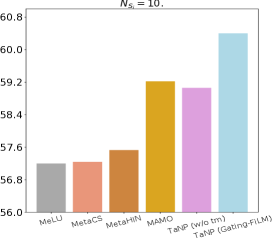
(a) MovieLens-1M

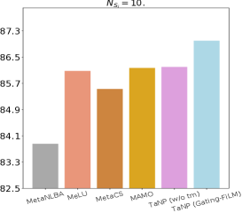
(b) Last.FM

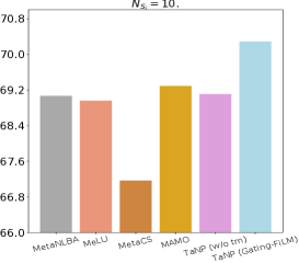
(c) Gowalla

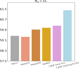
(d) MovieLens-1M

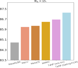
(e) Last.FM

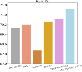
(f) Gowalla

Figure 3. Performance (%) comparison of user cold-start recommendation with different lengths of support set. The results of all datasets are provided. The first row shows the empirical results when $N_{S_{i}}=10$, and the second row shows the empirical results when $N_{S_{i}}=15$.

5.2.2. Compared Models

We compare our method with the following models:

• PPR (Park and Chu, 2009) is a well-known CF-based method to solve cold-start problems. PPR first constructs the profiles for user-item pairs by the outer product over their individual features, then it develops a novel regression framework to estimate the pairwise user preferences.

• NeuMF (He et al., 2017) is also a CF-based model that exploits DNNs to capture the non-linear feature interaction between user and item. NeuMF is a classic recommendation model, but it is not especially designed for cold-start problems. We adopt it here to test its effectiveness.

• DropoutNet (Volkovs et al., 2017) is a content-based model to solve cold-start problems. It applies the dropout mechanism to input during training to condition for missing user interactions.

• MetaLWA (Vartak et al., 2017) and MetaNLBA (Vartak et al., 2017) are the first meta-learning recommenders for cold-start problems. Different from our work, they focus on item cold-start recommendation. They generate two class-level prototype representations to learn item similarity. MetaLWA learns a linear classifier whose weights are determined by the user’s interaction history, and MetaNLBA learns a DNN with the task-dependent bias for each layer.

• MeLU (Lee et al., 2019) handles cold-start problems by applying the framework of MAML. Based on the learned parameter initialization, MeLU can make recommendations for cold-start users via a few steps of gradient updates.

• MetaCS (Bharadhwaj, 2019) is similar to MeLU, which also exploits MAML to estimate the user preference. It includes three model variants, and we choose the best one according to their reported results.

• MetaHIN (Lu et al., 2020) combines MAML with HINs to alleviate cold-start problems from model and data levels. The rich semantic of HINs provides a finer-grained prior which is beneficial to fast adaptations of new tasks.

• MAMO (Dong et al., 2020) is a memory-augmented framework of MAML. MAMO assumes that current MAML-based models often suffer from gradient degradation ending up with a local optima when handling users who show different gradient descent directions comparing with the majority of users in the training set. So it designs the task-specific and feature-specific memory matrices to solve this problem.

5.2.3. Implementation Details

The source codes of NeuMF , DropoutNet , MeLU , MetaHIN  and MAMO  have been released, and we modify the parts of data input and evaluations to fit our experimental settings. Other baselines are reproduced by ourselves. MetaLWA and MetaNLBA are only applicable to implicit feedback datasets, so the results of them on MovieLens-1M are not provided. While DropoutNet is a content-based method, the used input dropout is a general technique that can be also employed on Last.FM and Gowalla. In addition, both MetaHIN and MAMO are closely connected with the side-information of user and items. In particular, the meta-paths used in MetaHIN are constructed according to the node types of users, thus only the results of MetaHIN for MovieLens-1M are reported. The attention calculation in MAMO is obtained via user contents and the proposed profile memory. We replace this part with the original memory mechanism enabling MAMO to be deployed on Last.FM and Gowalla.

To make fair comparisons, the dimension sizes of user and item embeddings are fixed as 32 in embedding layers. All models are fully iterated with 150 epochs for convergence. In our model, the number of stacked layers $l$ for all modules in our model ($h_{\theta}$, $m_{\phi}$ and $g_{\omega_{i}}$) is 3, the learning rate is 5e-5 and the degree of freedom $\alpha$ is 1.0. Other hyper-parameters are selected according to the performances on validation datasets. The hidden size of each layer is selected from {8, 16, 32, 64, 128}, the hyper-parameter $\lambda$ in Eq.(19) is selected from {1.0, 0.5, 0.1, 0.05, 0.01}, and the number of soft cluster controids $k$ in the global pool $\bm{A}$ ranges from 10 to 50 with the step length 10.

5.3. Performance Comparison (RQ1)

Table 3, 4 and 5 demonstrate the performances of all models for user cold-start recommendation on MovieLens-1M, Last.FM and Gowalla. The size of support set $N_{S_{i}}$ is set as 20 in this section. The best performances are in bold. TaNP (w/o tm) denotes an ablation study of our model, in which the proposed task-adaptive mechanism is removed. TaNP (FiLM) and TaNP (Gating-FiLM) are two variants of our model using different modulation strategies. From these Tables, we can draw the following conclusions:

• TaNP consistently yields the best performances on all datasets. Compared with state-of-the-art meta-learning recommenders, the most obvious improvements of TaNP are listed here: for the MovieLens-1M, TaNP brings 4.2% improvements in terms of P@5; TaNP achieves 3.6% result lifts in terms of P@5 on Last.FM; For the Gowalla, TaNP provides 5.4% improvements in terms of MAP@5.

• Compared with those meta-learning recommenders based on MAML, we find that TaNP (w/o tm) achieves competitive performances. It demonstrates that our NP framework is suitable to user cold-start recommendation.

• In contrast to TaNP (w/o tm), the improvements of our variants, i.e., TaNP (FiLM) and TaNP (Gating-FiLM) are significant, and TaNP (Gating-FiLM) is slightly better than TaNP (FiLM). It demonstrates that the effectiveness of our task-adaptive mechanism and the importance of learning the relevance of different tasks.

• MetaLWA, MetaNLBA and MetaHIN are constrained by dataset types. Different from them, TaNP is a more general meta-learning recommender which can be used in different experimental settings.

5.4. Impact of $N_{S_{i}}$ (RQ2)

We change the number of interactions in $S_{i}$ for three datasets to test the effectiveness of our methods. Concretely, $N_{S_{i}}$ is set as 10 and 15 and the evaluation metric is P@10. According to the above results in Section 5.3, we select the following strong baselines: MetaNLBA, MeLU, MetaCS, MetaHIN and MAMO. Here we only report the results of TaNP (Gating-FiLM), since it achieves the better performances compared with TaNP (FiLM). The empirical results are provided in Figure 3, from which we can draw the following conclusions:

• For all datasets, when the number of interactions in the support set has been reduced, TaNP (Gating-FiLM) still maintains the better performances compared with other meta-learning models.

• TaNP (Gating-FiLM) performs better than TaNP (w/o tm) in all experimental settings. Compared with MeLU and MetaCS, the improvements of MAMO are also obvious. Through these two comparisons, we find that it is essential to use an effective adaptation for handling different tasks.

• Our model is less influenced by the decrease of interactions. The possible reason is that TaNP applies a random function to the constructions of $\tau_{i}$ for modeling different function realisations. In contrast, other baselines, such as the MetaNLBA and MetaCS, are more sensitive to the change of $N_{S_{i}}$.

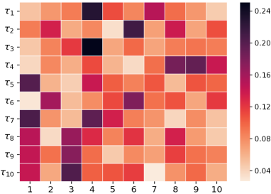
Figure 4. Visualization of soft cluster assignments of 10 tasks $\{\tau_{i}\}_{i=1}^{10}$. X axis represents $k=10$ cluster centroids. If $\tau_{i}$ and $\tau_{j}$ have high scores (i.e., dark color) on the same cluster centroids, we assume they may share some similarities.

5.5. Visual Analysis (RQ3)

In our model, the proposed adaptive mechanism includes a global pool $\bm{A}$ that implicitly represents $k$ cluster centroids to capture the relevance of different tasks. Each task $\tau_{i}$ would interact with $\bm{A}$ to derive the corresponding soft cluster assignments, and we randomly pick 10 tasks from the training set of MovieLens-1M with their corresponding soft cluster assignments. The visual result is shown in Figure 4, and we have the following conclusions:

• Our model can capture the similarity of tasks. For example, the highest normalized scores of $\tau_{5}$ and $\tau_{7}$ are simultaneously assigned to the first and the fourth clusters. We infer that these two tasks are closely relevant. The side-information also provide some cues. Concretely, we find the corresponding user ids $u_{5}$ and $u_{7}$ are of the same gender, and they share two movie items in support sets.

• The difference between tasks can be also well distinguished. For example, the soft assignments of $\tau_{1}$ and $\tau_{4}$ indicate that they are largely different.

Overall, the task relevance including the task similarity and the task difference is learned by the customization module. Moreover, such relevance is incorporated into the final task embedding which further facilitates the task-related modulations of decoder parameters reliably.

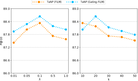
Figure 5. Empirical results of parameter sensitivity.

5.6. Hyper-parameter Analysis (RQ4)

In this section, we investigate the parameter sensitivity of our model with respect to two main hyper-parameters, i.e., $\lambda$ in the loss function and $k$ in $\bm{A}$. This experiment is conducted on Last.FM. As shown in Figure 5, TaNP (FiLM) achieves the best result when $\lambda=0.1$ and $k=10$, and TaNP (Gating-FiLM) achieves the best result when $\lambda=0.1$ and $k=20$. Thus, choosing relative small values of $\lambda$ and $k$ is sensible. In addition, two variants of our model are robust to the changes of $\lambda$ and $k$. Even in the worst cases of $\lambda$ and $k$, they are still better than other baselines shown in Table 4.

6. Conclusion

In this paper, we develop a novel meta-learning model called TaNP for user cold-start recommendation. TaNP is a generic framework which maps the observed interactions to the desired predictive distribution conditioned on a learned conditional prior. Furthermore, a novel task-adaptive mechanism is also introduced into TaNP for learning the relevance of different tasks as well as modulating the decoder parameters. Extensive results show that TaNP outperforms several state-of-the-art meta-learning recommenders consistently.

References

- (1)
- Antoniou et al. (2019) Antreas Antoniou, Harrison Edwards, and Amos Storkey. 2019. How to train your MAML. In International Conference on Learning Representations (ICLR).
- Bharadhwaj (2019) Homanga Bharadhwaj. 2019. Meta-Learning for User Cold-Start Recommendation. In 2019 International Joint Conference on Neural Networks (IJCNN).
- Bianchi et al. (2017) Mattia Bianchi, Federico Cesaro, Filippo Ciceri, Mattia Dagrada, Alberto Gasparin, Daniele Grattarola, Ilyas Inajjar, Alberto Maria Metelli, and Leonardo Cella. 2017. Content-based approaches for cold-start job recommendations. In Proceedings of the Recommender Systems Challenge.
- Blei et al. (2003) David M Blei, Andrew Y Ng, and Michael I Jordan. 2003. Latent dirichlet allocation. Journal of machine Learning Research (JMLR) (2003).
- Brockschmidt (2020) Marc Brockschmidt. 2020. Gnn-film: Graph neural networks with feature-wise linear modulation. In International Conference on Machine Learning (ICML).
- Cadene et al. (2019) Remi Cadene, Hedi Ben-Younes, Matthieu Cord, and Nicolas Thome. 2019. Murel: Multimodal relational reasoning for visual question answering. In IEEE Conference on Computer Vision and Pattern Recognition (CVPR).
- Cao* et al. (2021) Jiangxia Cao*, Xixun Lin*, Shu Guo, Luchen Liu, Tingwen Liu, and Bin Wang. 2021. Bipartite Graph Embedding via Mutual Information Maximization. In ACM International Conference on Web Search and Data Mining (WSDM).
- Das et al. (2007) Abhinandan S Das, Mayur Datar, Ashutosh Garg, and Shyam Rajaram. 2007. Google news personalization: scalable online collaborative filtering. In The World Wide Web Conference (WWW).
- Dong et al. (2020) Manqing Dong, Feng Yuan, Lina Yao, Xiwei Xu, and Liming Zhu. 2020. MAMO: Memory-Augmented Meta-Optimization for Cold-start Recommendation. In ACM Knowledge Discovery and Data Mining (KDD).
- Du et al. (2019) Zhengxiao Du, Xiaowei Wang, Hongxia Yang, Jingren Zhou, and Jie Tang. 2019. Sequential Scenario-Specific Meta Learner for Online Recommendation. In ACM Knowledge Discovery and Data Mining (KDD).
- Finn et al. (2017) Chelsea Finn, Pieter Abbeel, and Sergey Levine. 2017. Model-agnostic meta-learning for fast adaptation of deep networks. In International Conference on Machine Learning (ICML).
- Gao et al. (2018) Li Gao, Hong Yang, Jia Wu, Chuan Zhou, Weixue Lu, and Yue Hu. 2018. Recommendation with multi-source heterogeneous information. In International Joint Conference on Artificial Intelligence (IJCAI).
- Garnelo et al. (2018a) Marta Garnelo, Dan Rosenbaum, Chris J Maddison, Tiago Ramalho, David Saxton, Murray Shanahan, Yee Whye Teh, Danilo J Rezende, and SM Eslami. 2018a. Conditional neural processes. In International Conference on Machine Learning (ICML).
- Garnelo et al. (2018b) Marta Garnelo, Jonathan Schwarz, Dan Rosenbaum, Fabio Viola, Danilo Jimenez Rezende, S. M. Ali Eslami, and Yee Whye Teh. 2018b. Neural Processes. In International Conference on Machine Learning (ICML).
- Gordon et al. ([n.d.]) Jonathan Gordon, Wessel P Bruinsma, Andrew YK Foong, James Requeima, Yann Dubois, and Richard E Turner. [n.d.]. Convolutional conditional neural processes. In International Conference on Learning Representations (ICLR).
- Gu et al. (2010) Quanquan Gu, Jie Zhou, and Chris Ding. 2010. Collaborative filtering: Weighted nonnegative matrix factorization incorporating user and item graphs. In SIAM International Conference on Data Mining (SDM).
- He et al. (2017) Xiangnan He, Lizi Liao, Hanwang Zhang, Liqiang Nie, Xia Hu, and Tat-Seng Chua. 2017. Neural Collaborative Filtering. In The World Wide Web Conference (WWW).
- He et al. (2016) Xiangnan He, Hanwang Zhang, Min-Yen Kan, and Tat-Seng Chua. 2016. Fast matrix factorization for online recommendation with implicit feedback. In ACM International Conference on Research on Development in Information Retrieval (SIGIR).
- Kaiser et al. (2017) Łukasz Kaiser, Ofir Nachum, Aurko Roy, and Samy Bengio. 2017. Learning to remember rare events. In International Conference on Learning Representations (ICLR).
- Kim et al. (2019) Hyunjik Kim, Andriy Mnih, Jonathan Schwarz, Marta Garnelo, S. M. Ali Eslami, Dan Rosenbaum, Oriol Vinyals, and Yee Whye Teh. 2019. Attentive Neural Processes. In International Conference on Learning Representations (ICLR).
- Kingma and Ba (2015) Diederik P. Kingma and Jimmy Ba. 2015. Adam: A Method for Stochastic Optimization. In International Conference on Learning Representations (ICLR).
- Kingma and Welling (2014) Diederik P Kingma and Max Welling. 2014. Auto-encoding variational bayes. In International Conference on Learning Representations (ICLR).
- Koren et al. (2009) Yehuda Koren, Robert Bell, and Chris Volinsky. 2009. Matrix factorization techniques for recommender systems. Computer (2009).
- Kouki et al. (2015) Pigi Kouki, Shobeir Fakhraei, James Foulds, Magdalini Eirinaki, and Lise Getoor. 2015. Hyper: A flexible and extensible probabilistic framework for hybrid recommender systems. In ACM Conference on Recommender Systems (RecSys).
- Lee et al. (2019) Hoyeop Lee, Jinbae Im, Seongwon Jang, Hyunsouk Cho, and Sehee Chung. 2019. MeLU: Meta-Learned User Preference Estimator for Cold-Start Recommendation. In ACM Knowledge Discovery and Data Mining (KDD).
- Li et al. (2017) Zhenguo Li, Fengwei Zhou, Fei Chen, and Hang Li. 2017. Meta-sgd: Learning to learn quickly for few-shot learning. arXiv (2017).
- Liu et al. (2018) Chunyi Liu, Chuan Zhou, Jia Wu, Yue Hu, and Li Guo. 2018. Social recommendation with an essential preference space. In AAAI Conference on Artificial Intelligence (AAAI).
- Lops et al. (2011) Pasquale Lops, Marco De Gemmis, and Giovanni Semeraro. 2011. Content-based recommender systems: State of the art and trends. In Recommender Systems Handbook.
- Louizos et al. (2019) Christos Louizos, Xiahan Shi, Klamer Schutte, and Max Welling. 2019. The Functional Neural Process. In Annual Conference on Neural Information Processing Systems (NeurIPS).
- Lu et al. (2020) Yuanfu Lu, Yuan Fang, and Chuan Shi. 2020. Meta-learning on heterogeneous information networks for cold-start recommendation. In ACM Knowledge Discovery and Data Mining (KDD).
- Ma et al. (2019) Jianxin Ma, Chang Zhou, Peng Cui, Hongxia Yang, and Wenwu Zhu. 2019. Learning disentangled representations for recommendation. In Advances in Neural Information Processing Systems (NeurIPS).
- Ma et al. (2020) Jianxin Ma, Chang Zhou, Hongxia Yang, Peng Cui, Xin Wang, and Wenwu Zhu. 2020. Disentangled Self-Supervision in Sequential Recommenders. In ACM Knowledge Discovery and Data Mining (KDD).
- Mnih and Gregor (2014) Andriy Mnih and Karol Gregor. 2014. Neural variational inference and learning in belief networks. In International Conference on Machine Learning (ICML).
- Nichol and Schulman (2018) Alex Nichol and John Schulman. 2018. Reptile: a scalable metalearning algorithm. arXiv (2018).
- Oksendal (2013) Bernt Oksendal. 2013. Stochastic differential equations: an introduction with applications. Springer Science & Business Media.
- Park and Chu (2009) Seung-Taek Park and Wei Chu. 2009. Pairwise preference regression for cold-start recommendation. In ACM conference on Recommender systems (RecSys).
- Perez et al. (2018) Ethan Perez, Florian Strub, Harm De Vries, Vincent Dumoulin, and Aaron Courville. 2018. Film: Visual reasoning with a general conditioning layer. In AAAI Conference on Artificial Intelligence (AAAI).
- Ravi and Larochelle (2017) Sachin Ravi and Hugo Larochelle. 2017. Optimization as a model for few-shot learning. (2017).
- Requeima et al. (2019) James Requeima, Jonathan Gordon, John Bronskill, Sebastian Nowozin, and Richard E Turner. 2019. Fast and flexible multi-task classification using conditional neural adaptive processes. In Annual Conference on Neural Information Processing Systems (NeurIPS).
- Santoro et al. ([n.d.]) Adam Santoro, Sergey Bartunov, Matthew Botvinick, Daan Wierstra, and Timothy Lillicrap. [n.d.]. Meta-learning with memory-augmented neural networks. In International Conference on Machine Learning (ICML).
- Snell et al. (2017) Jake Snell, Kevin Swersky, and Richard Zemel. 2017. Prototypical networks for few-shot learning. In Annual Conference on Neural Information Processing Systems (NeurIPS).
- Vartak et al. (2017) Manasi Vartak, Arvind Thiagarajan, Conrado Miranda, Jeshua Bratman, and Hugo Larochelle. 2017. A meta-learning perspective on cold-start recommendations for items. In Annual Conference on Neural Information Processing Systems (NeurIPS).
- Vinyals et al. (2016) Oriol Vinyals, Charles Blundell, Timothy Lillicrap, Daan Wierstra, et al. 2016. Matching networks for one shot learning. In Annual Conference on Neural Information Processing Systems (NeurIPS).
- Volkovs et al. (2017) Maksims Volkovs, Guangwei Yu, and Tomi Poutanen. 2017. Dropoutnet: Addressing cold start in recommender systems. In Advances in Neural Information Processing Systems (NeurIPS).
- Vuorio et al. (2019) Risto Vuorio, Shao-Hua Sun, Hexiang Hu, and Joseph J Lim. 2019. Multimodal Model-Agnostic Meta-Learning via Task-Aware Modulation. In Annual Conference on Neural Information Processing Systems (NeurIPS).
- Wang and Blei (2011) Chong Wang and David M Blei. 2011. Collaborative topic modeling for recommending scientific articles. In ACM Knowledge Discovery and Data Mining (KDD).
- Wang et al. (2015) Hao Wang, Naiyan Wang, and Dit-Yan Yeung. 2015. Collaborative deep learning for recommender systems. In ACM Knowledge Discovery and Data Mining (KDD).
- Wang et al. (2019) Hongwei Wang, Fuzheng Zhang, Miao Zhao, Wenjie Li, Xing Xie, and Minyi Guo. 2019. Multi-task feature learning for knowledge graph enhanced recommendation. In The World Wide Web Conference (WWW).
- Xie et al. (2016) Junyuan Xie, Ross Girshick, and Ali Farhadi. 2016. Unsupervised deep embedding for clustering analysis. In International Conference on Machine Learning (ICML).
- Xin and Jaakkola (2014) Yu Xin and Tommi Jaakkola. 2014. Controlling privacy in recommender systems. In Annual Conference on Neural Information Processing Systems (NeurIPS).
- Yao et al. (2019) Huaxiu Yao, Ying Wei, Junzhou Huang, and Zhenhui Li. 2019. Hierarchically structured meta-learning. In International Conference on Machine Learning (ICML).
- Zhang et al. (2019) Shuai Zhang, Lina Yao, Aixin Sun, and Yi Tay. 2019. Deep learning based recommender system: A survey and new perspectives. ACM Computing Surveys (CSUR) (2019).
- Zheng et al. (2016) Yin Zheng, Bangsheng Tang, Wenkui Ding, and Hanning Zhou. 2016. A neural autoregressive approach to collaborative filtering. In International Conference on Machine Learning (ICML).