Torsional rigidity for tangential polygons

Abstract

An inequality on torsional rigidity is established. For tangential polygons this inequality is stronger than an inequality of Polya and Szego for convex domains. (A survey of related work, not in the journal submission, is presented.)

1 Introduction

In the most general situation $\Omega$ is a simply-connected plane domain. However as we wish to compare our inequalities with earlier results proved for convex domains, notably the Polya-Szego inequality (involving equation (1.3)), we have in mind convex domains. Although Theorem 1 concerns more general domains, our main result derived from it, Theorem 2, concerns tangential polygons. We will denote the area of $\Omega$, $|\Omega|$, by $A$, and its perimeter $|\partial\Omega|$ by $L$.

1.1 The torsion pde, Problem (P(0))

The elastic torsion problem is to find a function $u_{0}$ satisfying

$$-\frac{\partial^{2}u_{0}}{\partial x^{2}}-\frac{\partial^{2}u_{0}}{\partial y^{2}}=1\,{\rm in}\,\Omega,\,\qquad u_{0}=0\,{\rm on}\,\partial\Omega\,.$$

Define the torsional rigidity of $\Omega$ as,

$$Q_{0}:=\int_{\Omega}u_{0}.$$ (1.1)

(This differs by a factor of 4 from definitions elsewhere, e.g in [69].) There are many identities and inequalities concerning $Q_{0}$. For example, one identity is

$$Q_{0}=\frac{1}{4}\,\int_{\partial\Omega}(x.n)\left(\frac{\partial u_{0}}{\partial n}\right)^{2}.$$ (1.2)

Define (for convex $\Omega$), in the notation of [69],

$$B_{\Omega}=\int_{\partial\Omega}\frac{1}{x\cdot{n}}.$$ (1.3)

An inequality, which we will call the Polya-Szego inequality, is

$$Q_{0}\geq\frac{A^{2}}{4\ B_{\Omega}}(={\rm{\ for\ tangential\ polygons\ }}\frac{A^{3}}{2L^{2}})$$ (1.4)

Define

$$J(v)=\int_{\Omega}\left(2v-|\nabla v|^{2}\right).$$

The solution $u_{0}$ maximizes $J$ over functions vanishing on the boundary $\partial\Omega$. (More precisely over functions $v\in{{\mathring{W}}^{1}_{2}(\Omega)}$.)

A quantity occuring in our Theorem 1 is

$$Q_{1}=\int_{\partial\Omega}\left(\frac{\partial u_{0}}{\partial n}\right)^{2}.$$ (1.5)

For tangential polygons from equation (1.2) we note that there is a very simple equation relating $Q_{1}$ and $Q_{0}$: this is needed for our Theorem 2.

1.2 Problem (P($\infty$))

Problem (P($\infty$) was defined in the statement of Theorem 2.2 of [44]. Our notation here is as in that paper. where $u_{\infty}$ solves

$$-\frac{\partial^{2}u_{\infty}}{\partial x^{2}}-\frac{\partial^{2}u_{\infty}}{\partial y^{2}}=1\,{\rm in}\,\Omega,\,\frac{\partial u_{\infty}}{\partial n}=-\frac{|\Omega|}{|\partial\Omega|}\,{\rm on}\,\partial\Omega\,{\rm and}\,\int_{\partial\Omega}u_{\infty}=0.$$

Define, as in [44] equations (4.9) and (4.11),

$$\Sigma_{\infty}=\int_{\Omega}u_{\infty},\qquad{\rm and\ \ }\Sigma_{1}=-\int_{\partial\Omega}u_{\infty}^{2},$$ (1.6)

with $u_{\infty}$ satisfying Problem (P($\infty$)).

Once again there is a variational characterisation of the solutions. This time $u_{\infty}$ is the maximizer of $J(v)$ as one varies over functions $v$ for which the integral of $v$ over the boundary $\partial\Omega$ is zero. The variational approach can be used to establish the inequality

$$\Sigma_{\infty}\geq Q_{0}.$$ (1.7)

(See also [44] equation (4.9) for a different approach.)

The solution $u_{\infty}$ when $\Omega$ is a tangential polygon is given in [44] equations (2.14) and (2.15).

2 Relations between $u_{0}$ and $u_{\infty}$

We already have (1.7) relating $\Sigma_{\infty}$ and $Q_{0}$. The next result involves $\Sigma_{1}$ and $Q_{1}$. (We haven’t exp[ored to what extent the boundary smoothness might be relaxed. We need to apply the Divergence Theorem.)

Theorem 1

For (convex) domains $\Omega$ with Lipschitz boundary which is also piecewise $C^{1}$, the following inequality is satisfied:

$$\frac{A^{2}}{L}-\frac{(\Sigma_{\infty}-Q_{0})^{2}}{\Sigma_{1}}\leq Q_{1}.$$ (2.1)

Recall that $\Sigma_{1}<0$, so both terms on the left-hand side are positive.

Proof. Considering ${\rm div}(u_{0}\nabla u_{\infty})$ the Divergence Theorem gives

$$Q_{0}=\int_{\Omega}\nabla u_{0}\,\cdot\,\nabla_{\infty}.$$

Considering ${\rm div}(u_{\infty}\nabla u_{0})$ the Divergence Theorem gives

$$\int_{\partial\Omega}u_{\infty}\frac{\partial u_{0}}{\partial n}=-\Sigma_{\infty}+\int_{\Omega}\nabla u_{0}\,\cdot\,\nabla u_{\infty}.$$

These combine to give

$$\Sigma_{\infty}-Q_{0}=\int_{\partial\Omega}u_{\infty}\left(-\frac{\partial u_{0}}{\partial n}\right).$$

We now introduce an arbitrary constant $c$ and subtract $c\,A$ from both sides, giving

$$(\Sigma_{\infty}-Q_{0})-cA=\int_{\partial\Omega}(u_{\infty}-c)\,\left(-\frac{\partial u_{0}}{\partial n}\right).$$ (2.2)

We now use the Cauchy-Schwarz inequality on the right-hand side to give

$$\left((\Sigma_{\infty}-Q_{0})-cA\right)^{2}\leq Q_{1}\,\int_{\partial\Omega}(u_{\infty}-c)^{2},$$

where we have used equation (3.1) for one of the integrals on the right-hand side. Now, on using that the integral of $u_{\infty}$ around the boundary is zero, we have

$$\int_{\partial\Omega}(u_{\infty}-c)^{2}=-\Sigma_{1}+c^{2}L.$$

Thus, for all real $c$

$$\frac{\left((\Sigma_{\infty}-Q_{0})-cA\right)^{2}}{-\Sigma_{1}+c^{2}L}\leq Q_{1}$$ (2.3)

The function of $c$ on the left is clearly nonnegative and bounded, tending to $A^{2}/L$ as c tends to both plus and minus infinity. It has two critical points: the one making the function 0 is clearly the minimum. The other is at $c=c_{*}$ where

$$c_{*}=\frac{A\Sigma_{1}}{L(\Sigma_{\infty}-Q_{0})}.$$

Subsitituting $c_{*}$ for $c$ in inequality (2.3) yields the result of the theorem. $\square$

3 Tangential polygons

3.1 Geometric results

A tangential polygon, also known as a circumscribed polygon, is a convex polygon that contains an inscribed circle (also called an incircle), a circle that is tangent to each of the polygon’s sides. For any (convex) tangential polygon, the area $A$, perimeter $L$ and inradius $\rho$ are related by

$$A=\frac{1}{2}\rho L.$$

We always choose the origin of our coordinate system to be at the incentre. There is some literature on tangential polygons, e.g. [2, 74]. Any triangle is a tangential polygon. Quadrilaterals which are tangential include kites and hence rhombi.

Concerning $B$, defined in [69] and here at equation (1.3), another simple identity for (convex) tangential polygons is

$$B=\frac{L}{\rho},$$

(and $B\geq{2\pi}$ with equality only for the disk, and for any triangle, $B\geq{6\sqrt{3}}$): see [1].

The quantities $\Sigma_{\infty}$ and $\Sigma_{1}$ can be expressed in terms of boundary moments $i_{2k}$ – moments about the incentre – defined by

$$i_{2k}=\int_{\partial\Omega}(x^{2}+y^{2})^{k}.$$

We remark that the Cauchy-Schwarz inequality for the integrals implies that $i_{4}\geq{i_{2}^{2}/L}$.

For methods to calculate $i_{2k}$ in terms of the tangential polygon’s inradius and angles, see [47].

3.2 The new inequality for tangential polygons

Since on the boundary $\partial\Omega$ of a tangential polygon we have $x\cdot{n}=\rho$, equation (1.2) yields, for tangential polygons,

$$Q_{0}=\frac{\rho}{4}\int_{\partial\Omega}\left(\frac{\partial u_{0}}{\partial n}\right)^{2}.$$ (3.1)

This enables us to rewrite the preceding theorem as follows.

Theorem 2

For any tangential polygon $Q_{0}$ satisfies the inequality, quadratic in $Q_{0}$,

$$\frac{A^{2}}{L}-\frac{(\Sigma_{\infty}-Q_{0})^{2}}{\Sigma_{1}}\leq\frac{4}{\rho}Q_{0}.$$ (3.2)

In our application we treat inequality (3.2) as a quadratic inequality in $Q_{0}$ and it is satisfied if

$$Q_{0-}\leq Q_{0}\leq Q_{0+},$$

where, with

$$\delta=-\frac{\Sigma_{1}}{L}\left(2AL^{2}\Sigma_{\infty}-L^{3}\Sigma_{1}-A^{4}\right),$$

$$Q_{0\pm}=\frac{1}{A}\left(-L\Sigma_{1}+A\Sigma_{\infty}\pm\sqrt{\delta}\right).$$

3.3 $\Sigma_{\infty}$ and $\Sigma_{1}$

For a tangential polygon

$$u_{\infty}=c_{0}-\frac{1}{4}r^{2}\qquad{\rm where\ }r^{2}=x^{2}+y^{2},\ {\rm and\ \ }c_{0}=\frac{i_{2}}{4L}.$$ (3.3)

$c_{0}$ is such that the boundary integral is zero. This was noted at equations (2.14), (2.15) of [44]. We find

$$\Sigma_{\infty} = \frac{1}{16}\rho i_{2}=\frac{Ai_{2}}{8L},$$ (3.4)

$$\Sigma_{1} = -c_{0}^{2}\,L+\frac{1}{2}c_{0}i_{2}-\frac{1}{16}i_{4}=\frac{1}{16}\left(\frac{i_{2}^{2}}{L}-i_{4}\right).$$ (3.5)

We can now readily rewrite our inequality (3.2) in terms of the geometric quantities $i_{2}$ and $i_{4}$. Using the expressions (3.4,3.5) in terms of $i_{2}$, $i_{4}$ we find that the inequality of (3.2) is satisfied iff the following inequality, quadratic in $Q_{0}$, is satisfied

$$f(Q_{0}):=32AQ_{0}^{2}-\frac{4Q_{0}}{\rho}\left(2Ai_{4}-\rho i_{2}^{2}+Ai_{2}\rho^{2}\right)+A\rho\,(Ai_{4}-\frac{3}{8}i_{2}^{2}\rho)\leq{0}\ .$$ (3.6)

Inequalities on the domain functionals $A$, $\rho$, $i_{2}$ and $i_{4}$ can be used to establish that both roots of $f(Q_{0})=0$ are positive. Denote the smaller root by $Q_{0-}$ and the larger by $Q_{0+}$. The inequalities $Q_{0-}\leq Q_{0}\leq Q_{0+}$ improve, for tangential polygons, some well known inequalities such as the Polya-Szego inequality (1.4),

$$Q_{0}\geq\frac{A^{2}}{4\ B_{\Omega}}(={\rm{\ for\ tangential\ polygons\ }}\frac{A^{3}}{2L^{2}}=\frac{\rho^{2}A}{8}).$$

We now comment on the quadratic $f$. Consider first a disk radius 1

$$A_{\odot}=\pi,\ \rho_{\odot}=1,\ i_{2,\odot}=i_{4,\odot}=2\pi,$$

$\mathrm{so}{f}_{\odot }(Q_0)=32\pi Q_0^2-4Q_0(2{\pi }^2)+{\displaystyle \frac{1}{2}}{\pi }^3=32\pi {(Q_{0-}{\displaystyle \frac{\pi }{8}})}^2.$

This agrees with that $Q_{0,\odot}=\pi/8$. Next consider an equilateral triangle,

$$A_{\Delta}=\sqrt{3},\ \rho_{\Delta}=\frac{1}{\sqrt{3}},\ i_{2,\Delta}=4,\ i_{4,\Delta}=\frac{16}{5},$$

$\mathrm{so}{f}_{\mathrm{\Delta }}(Q_0)=32\sqrt{3}{Q}_0^2-4Q_0\sqrt{3}({\displaystyle \frac{12\sqrt{3}}{5}})+{\displaystyle \frac{6\sqrt{3}}{5}}=32\sqrt{3}(Q_{0-}{\displaystyle \frac{\sqrt{3}}{20}})(Q_0-{\displaystyle \frac{\sqrt{3}}{4}}),$

which is consistent with $Q_{0,\Delta}=\sqrt{3}/20$.

Consider next general tangential polygons. Define $Q_{B}=\rho^{2}A/8$, and recall the Polya-Szego inequality $Q_{0}\geq Q_{B}$. We have

$$f(Q_{B})=\frac{\rho^{2}A}{2}\left(\rho A-\frac{1}{2}\rho i_{2}\right)^{2}.$$

Thus the inequality $Q_{0}\geq Q_{0-}$ improves on $Q_{0}\geq Q_{B}$. Consider next the upper bound $Q_{0}\leq{I_{O}/4}$ where $I_{O}$ is the polar moment of inertia about the incentre $O$, which can also be written $Q_{0}\leq\Sigma_{\infty}$. Then $I_{O}=4\Sigma_{\infty}=\rho i_{2}/4$ and

$$f(\frac{1}{16}\rho i_{2})=-\frac{1}{2}\left(\frac{i_{2}}{2}-\rho A\right)\,\left(2Ai_{4}-\rho i_{2}^{2}\right).$$

Since both terms in parentheses are positive, one concludes that $\rho i_{2}/16\leq Q_{0+}$ so the bound $Q_{0}\leq Q_{0+}$ is weaker than the earlier bound. Summarizing, we have

$$Q_{B}=\frac{1}{8}\rho^{2}A\leq Q_{0-}\leq Q_{0}\leq\frac{1}{16}\rho i_{2}\leq Q_{0+}.$$

Using the calculations of $\Sigma_{\infty}$ and $\Sigma_{1}$ for isosceles triangles with area $\sqrt{3}$ given in  Part II  we show in Figure 1 how the new inequality compares with earlier inequalities. As another check we note that perhaps the most studied isosceles triangle other than the equilateral is the right isosceles triangle. Let $\alpha$ be the apex angle of the isosceles triangle and $\sigma=\tan(\alpha/4)$ so $0<\sigma<1$. For this $\sigma=\sqrt{2}-1\approx{0.414214}$ and for area $\sqrt{3}$ its torsional rigidity is approximately 0.07827 (see [69]) which is, as it must be, larger than $Q_{0-}$ which, at this $\sigma$, is 0.076511. However, at just 2.5% difference, it is too close to the curve to plot usefully.

4 Conclusion, and open problems

There are many questions.

We do not know if inequality (2.1) is implied by some other known inequality for torsional rigidity.

Inequality (3.2) becomes an equality for circular disks and equilateral triangles. It may be that these are the only shapes which achieve this.

For isosceles triangles with a given area, as indicated in Figure 1, $Q_{0-}$ is maximized (and $Q_{0+}$ minimized) by the equilateral triangle. We believe that this will be true for all triangles. What happens with quadrilaterals, and more generally $n$-gons, is not known.

It would also be possible to check how well the inequality checks with computed torsional rigidities for polygons, a few references being [32, 75, 79]. Perhaps checking for the regular polygons where the data is given in Table 1 of  Part II would be the easiest place to start.

To date the work has been on domains for which $u_{\infty}$ is a quadratic polynomial. ([50] treats rectangles.) Outside this class of domains, there are other domains for which all the functionals in inequality (2.1) can be found, for example, the semi-circle has elementary function solutions for both $u_{0}$ and $u_{\infty}$ and the various functionals can be found (using Maple to sum the series).

Structure of the remainder of this document

The preceding part of this document, called Part I from now on, has been accepted, subject to revision, for publication in IMA Journal of Applied Mathematics.
One referee was very positive and concluded:
“This paper too is very well written, clear, and easy to follow. I strongly recommend publication in IMA Journal of Applied Mathematics”
The other referee wrote of the paper:
“the work was not put into context and background/other related studies were not discussed …. I think it’d be good to discuss previous work on this topic, so that it is clear what the new contribution of this work is. The derived inequalities will be interesting once a discussion is given (e.g of other inequalities which have appeared in the literature, why are these important etc.). ”
The same referee also suggested:
“computing torsional rigidities for specific cases and comparing to other studies”.
This supplement is intended to address this, while leaving the journal paper short and focussed on the new research.
Numerics for the torsional rigidities of regular polygons and of isosceles triangles (in the papers submitted to IMA) are repeated here in Parts I and IIa. Additional numerics for rhombi are given near the end of Part III.

• The earlier part of this document, Part I, is a preprint form of the IMA paper. Some items addressing a referee’s concerns with the original form or the paper are in Part Ib.

• Part II concerns geometric matters relating to tangential polygons.
  Part IIa is adapted from material used in a different context in the paper [47]
  Part IIb contains geometric items not in the IMA paper(s).
  The first topics are related to $n$-gons including‘isoperimetric inequalities’, when, with the number of vertices $n$ fixed, with some fixed parameter (e.g. area) regular polygons optimize over some other parameter (e.g. minimize the perimeter).
  A second topic is inequalities, sometimes not involving $n$ or at least allowing $n$ to range over positive integers, ‘circumgons’ and ‘circum-$n$-gons’, i.e. shapes in which part of the boundary is the disk with radius the inradius. One of these is the ‘single-cap’, the convex hull of the disk and a single point outside it: a circum-1-gon. Another is the ‘symmetric double-cap’: a circum-2-gon. We will see these in connection with Blaschke-Santalo diagrams.

• In Part III we return to considerations of torsional rigidity. The emphasis is on bounds for convex domains, in particular convex polygons especially tangential polygons. Some sections are devoted to triangles, especially isosceles, and tangential quadrilaterals, especially rhombi.

• The remaining parts are only slightly connected to the torsion problem.
  Part IV concerns replacing the Dirichlet b.c. with a Robin b.c..
  Part V notes some other pde problems where tangential polygons are mentioned.

The treatment is very uneven. I have not checked the more advanced recent pde papers. Some of the geometry papers cited in Part II are very elementary. The suggestion (by Buttazzo) that I look at Blaschke-Santalo diagrams has led to items at present poorly integrated with the study of my bound $Q_{0-}$ (with just Part III §27 indicating one direction). I hope a later version of this supplement will correct some of these defects.

Part Ib

Numerics for the isosceles triangle

Numerics for the isosceles triangle were described earlier, but here is some amplification.

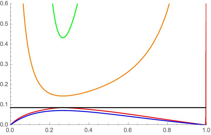
Figure 1: For an isosceles triangle with area$\sqrt{3}$. $\sigma$ is tan of 1/4 of the apex angle. Blue is $Q_{B}$, red is the new lower bound $Q_{0-}$, black is $Q_{\Delta}$, orange is $\rho i_{2}/16$, green is $Q_{0+}$.

Another lower bound on $Q_{0}$, as in [82], is that, amongst triangles with a given inradius, the equilateral triangle has the smallest $Q_{0}$. Thus

$$Q_{0}\geq Q_{\rm Sol}=\frac{9\sqrt{3}}{20}\rho^{4}.$$ (4.1)

For isosceles triangles this lower bound improves on our $Q_{0-}$ when the apex angle is slightly less than $\pi/3$. See Figure 2.

Figure 2: A plot, against $\sigma$, of the difference $Q_{0-}-Q_{\rm Sol}$, the latter term defined in equation(4.1).

Speculation on equality in inequality (3.2).

Inequality (3.2) becomes an equality for circular disks and equilateral triangles. I don’t have a proof, but it might be that one only gets equality for these shapes.

There is just one inequality used in the proof of the theorems. It is a Cauchy-Schwarz Inequality and it will be an equality iff

$$u_{\infty}-c_{*}={\rm const}\,\frac{\partial u_{0}}{\partial n},$$

all the way around the boundary. The lhs is a quadratic function of $(x,y)$. Consider next a genuine polygon, a tangential $n$-gon. Without loss of generality consider a side parallel to the $x$-axis as the interval $-1\leq{x}\leq{1}$, and $y=-h$, with the $n$-gon being in the half-plane $\{y>-h\}$. The only possibility is

$$\frac{\partial u_{0}}{\partial y}=-\frac{1}{4}(1-x^{2}),\qquad{\rm on\ }y=-h,\ \ -1<x<1,$$

as the gradient of $u_{0}$ is zero at the corners. This has implications for the values of $c_{0}$ in $u_{\infty}$ and $c_{*}$. Further information might be obtained by considering sides adjoining the $y=-h$ side, with angles $\alpha_{-}$ at $x=-1$ and $\alpha_{+}$ at $x=1$. One might get other restrictions on the $c_{0}$ and $c_{*}$ values, and on the $\alpha\pm$.

Even if the disk and equilateral triangle are the only bounded domains for which we get equality, it might be difficult to show this. If one considers an infinite wedge as ‘tangential polygon’ this might be a counterexample. Consider a wedge, apex at the origin and symmetric about the $x$-axis, $\theta=0$. Suppose that the wedge has angle $\alpha$. Then

$$u_{0,{\rm wedge}}=-\frac{r^{2}}{4}\left(1-\frac{\cos(2\theta)}{\cos(\alpha)}\right)+{\rm const}r^{\pi/\alpha}\cos(\pi\frac{\theta}{\alpha}),$$

solves the torsion equation, has zero Dirichlet boundary data. Here

$$\frac{\partial u_{0}}{\partial n}=\frac{1}{r}\frac{\partial u_{0}}{\partial\theta}.$$

It might be that we can set the const to 0 to see a counter example. (The solution in a sector is given in [43].)

Part IIa: $\Sigma_{\infty}$ and $\Sigma_{1}$ for tangential polygons

Abstract for Part IIa

Items useful in calculation for tangential polygons in general, and for particular cases, are here extracted from [47].

5 Outline of Part IIa

In this part the functionals $\Sigma_{\infty}$ and $\Sigma_{1}$ are calculated for various tangential polygons. The starting point is equation (2.14), (2.15) from the 1993 paper [44] – repeated at appropriate times in this document – which gives $u_{\infty}=c_{0}-\frac{1}{4}(x^{2}+y^{2})$ for tangential polygons, with $c_{0}$ such that the boundary integral of $u_{\infty}$ is 0.

• In §6 we find that starting from $u_{\infty}$ the functionals $\Sigma_{\infty}$ and $\Sigma_{1}$ can be expressed in terms of various moments of inertia.

• In §7 we treat the circular disk and the equilateral triangle.

• In §8 we study regular $n$-gons.

• Any triangle is a tangential polygon.
  In §9 we find the functionals for any isosceles triangle.

• In §10. we note papers relevant to work on tangential quadrilaterals.

We will use ‘tangential polygon’ as defined before.

• Genuine $n$-sided polygons for which every side is tangent to the incircle (and hence for which the intersection of the boundary with the incircle is $n$ points, the points of tangency) will be called tangential $n$-gons.

• When tangential polygon is the convex hull of $n$ points outside the incircle and the incircle we will call it a circum-$n$-gon. (This is a slightly different terminology than in [2].

Tangential $n$-gons are particular cases of circum-$n$-gons. The union over all $n$ from 0 to $\infty$ of circum-$n$-gons gives all tangential polygons (the $n=0$ case being considered as the disk). A circum-1-gon is also called a 1-cap, a circum-2-gon is also called a 2-cap: we will see these in Part IIb.

We use established terminology with a circum-4-gon being called a tangential quadrilateral, a circum-6-gon a tangential hexagon, etc.

6 Tangential polygons

6.1 Geometric results

Here we continue from the basic geometric definitions and results given in Part IIa §5.

There are various well-known or elementary observations:

• Of the polygons with fixed perimeter and angles, the tangential polygon has the greatest area.

• Given two (convex) tangential polygons with the same incircle their intersection is also a (convex) tangential polygon with the same incircle.

Papers concerning tangential polygons include [2, 74] (and many more particularly concerning tangential $n$-gons for $3\leq{n}\leq{6}$ will be given at appropriate places later in this document). There is a literature on (convex) tangential polygons, one fact being that, considering the polygons as linkages touching the incircle, if the number of sides is odd the polygon is rigid but not if the number of sides is even. Entertaining as such facts are, they do not appear to be relevant to our pde exercise.

We will need boundary moments $i_{2k}$ – moments about the incentre – defined by

$$i_{2k}=\int_{\partial\Omega}(x^{2}+y^{2})^{k},$$

and the polar area moment about the incentre

$$I_{2k}=\int_{\Omega}(x^{2}+y^{2})^{2}.$$

(Caution. There are many results concerning moments about the centroid. For example, as in [69], the moments about the centroid are minimized over $n$-gons with a given fixed area by the regular $n$-gon. We haven’t checked in general if it is the case that the moments about the incentre are minimized over $n$-gons by the regular $n$-gon, but when $n=3$ and one minimizes over isosceles triangles, the equilateral triangle is the minimizer.)

We remark that the Cauchy-Schwarz inequality for the integrals implies that $i_{4}\geq{i_{2}^{2}/L}$ (and $I_{4}\geq{I_{2}^{2}/A}$).

6.1.1 $I_{2k}=\rho\,i_{2k}/(2k+2)$.

A result which we first noticed in two special cases is the following.

Result. For any tangential polygon $A=\rho\,L/2$, $I_{2}=\rho\,i_{2}/4$ and, more generally, $I_{2k}=\rho\,i_{2k}/(2k+2)$.

Proof. The Divergence Theorem can be used to give a boundary integral which equals $I_{2}$. Consider polar coordinates, radial coordinate $r$, and the Laplacian of a function of $r$:

$$\Delta u=\frac{1}{r}\frac{\partial}{\partial r}r\frac{\partial u}{\partial r}.$$

Also, for use in the following, for any tangential polygon $x.n=\rho$, here $x$ being the vector to a point on $\partial\Omega$. To avoid using $x$ as a vector, equally $re_{r}.n=\rho$, with $e_{r}$ the unit vector in the $r$-direction.

With $u=r^{2}$ so $\Delta r^{2}=4$ the Divergence Theorem gives

$$2\rho L=\int_{\partial\Omega}2re_{r}.n=\int_{\Omega}4=4A.$$

Similarly, with $u=r^{4}$ so $\Delta r^{4}=16r^{2}$ the Divergence Theorem gives

$$4\rho i_{2}=\int_{\partial\Omega}(\nabla r^{4}).n=\int_{\Omega}16\,r^{2}=16I_{2}.$$

Alternative Proof. Start with a tangential polygon $T(1)$ origin at the incentre, with radius 1. Define $T(\rho)=\rho\,T(1)$ with second area moment $I_{2}(\rho)$ and second boundary moment $i_{2}(\rho)$. Along with $T(\rho)$ consider a similar scaled polygon $T(\rho+\Delta\rho)$ with $\Delta\rho$ small. Then

$$I_{2}(\rho+\Delta\rho)-I_{2}(\rho)\sim\Delta\rho\,i_{2}(\rho)+O((\Delta\rho)^{2}).$$

But, dimensionally, $i_{2}(\rho)=\rho^{3}\,i_{2}(1)$ and $I_{2}(\rho)=\rho^{3}\,I_{2}(1)$. Taking limits in the displayed equation gives the central part of

$$4\rho^{3}I_{2}(1)=\frac{dI_{2}(\rho)}{d\rho}=i_{2}(\rho)=\rho^{3}i_{2}(1).$$

This gives $i_{2}(1)=4I_{2}(1)$ and hence, more generally, $I_{2}(\rho)=\rho\,i_{2}(\rho)/4$ as asserted.

The same methods give $I_{2k}=\rho\,i_{2k}/(2k+2)$, and the case $k=0$ is $A=\rho\,L/2$.

6.1.2 Methods to calculate $i_{2k}$.

Denote with a bar just contributions from a vertical side, at $x=\rho$, extending from $y=-\eta_{-}$ to $y=\eta_{+}$. Then

$${\bar{i}}_{2k}=\int_{-\eta_{-}}^{\eta_{+}}(\rho^{2}+y^{2})^{k}\,dy.$$

Hence

$${\bar{i}}_{0} = \eta_{+}+\eta_{-},$$

$${\bar{i}}_{2} = \rho^{2}{\bar{i}}_{0}+\frac{1}{3}(\eta_{+}^{3}+\eta_{-}^{3}),$$

$${\bar{i}}_{4} = -\rho^{4}{\bar{i}}_{0}+2\,\rho^{2}{\bar{i}}_{2}+\frac{1}{5}(\eta_{+}^{5}+\eta_{-}^{5}).$$

Assuming the tangential polygon has $n$ sides, this gives

$${i}_{0}=L = \sum_{k=1}^{n}(\eta_{k+}+\eta_{k-}),$$ (6.1)

$${i}_{2} = \rho^{2}{i}_{0}+\frac{1}{3}\sum_{k=1}^{n}(\eta_{k+}^{3}+\eta_{k-}^{3}),$$ (6.2)

$${i}_{4} = -\rho^{4}{i}_{0}+2\,\rho^{2}{i}_{2}+\frac{1}{5}\sum_{k=1}^{n}(\eta_{k+}^{5}+\eta_{k-}^{5}).$$ (6.3)

There is the geometrically evident fact that $\eta_{k+}=\eta_{k+1,-}$ as one traverses from one of the polygon’s sides to the next.

The easiest case to consider is the regular $n$-gon, side $s_{n}=2\rho\tau_{n}$ where $\tau_{n}=\tan(\pi/n)$. Then

$${i}_{0}=L = n\,s_{n}=2n\rho\tau_{n},$$ (6.4)

$${i}_{2} = \rho^{2}{i}_{0}+\frac{n}{12}s_{n}^{3}=n\,s_{n}\left(\rho^{2}+\frac{1}{12}s_{n}^{2}\right)=\frac{2}{3}n\rho^{3}\tau_{n}(3+\tau_{n}^{2}),$$ (6.5)

$${i}_{4} = -\rho^{4}{i}_{0}+2\,\rho^{2}{i}_{2}+\frac{n}{80}s_{n}^{5}=n\,s_{n}\left(\rho^{4}+\frac{\rho^{2}s_{n}^{2}}{6}+\frac{s_{n}^{4}}{80}\right),$$ (6.6)

$$= \frac{2}{15}n\rho^{5}\tau_{n}\left(15+10\,\tau_{n}^{2}+3\,\tau_{n}^{4}\right).$$ (6.7)

These had been calculated independently from first principles, as reported in §8.1, before our observations concerning general tangential polygons.

We now consider how $\eta_{+}$ and $\eta_{-}$ might be found in terms of vertex angles of the tangential polygon. Recall that in any tangential polygon the angle bisector at any vertex passes through the incentre. Suppose side $k$ lies between vertices $k$ and $k+1$. Let the angle at vertex $k$ be $\alpha_{k}$. (If there are $n$ sides the sum over all the $\alpha_{k}$ is $(n-2)\pi$.) Then, with

$$T_{k}=\frac{1}{\tan\frac{\alpha_{k}}{2}}=\tan(\frac{\pi-\alpha_{k}}{2}),$$ (6.8)

$$\eta_{k-}={\rho}T_{k},\qquad\eta_{k+}=\rho T_{k+1}.$$

Summing over $k$

$$A=\rho^{2}{\sum\atop{k}}T_{k},\qquad L=2\rho{\sum\atop{k}}T_{k}.$$ (6.9)

(This checks with our previous $A=\rho L/2$.) Another well-known identity is

$$\frac{L^{2}}{4A}={\sum\atop{k}}T_{k}.$$

Similarly

$${i}_{2} = \rho^{2}{i}_{0}+\frac{2\rho^{3}}{3}\sum_{k=1}^{n}T_{k}^{3}=2\rho^{3}\,\sum_{k=1}^{n}\left(T_{k}+\frac{T_{k}^{3}}{3}\right),$$ (6.10)

$${i}_{4} = -\rho^{4}{i}_{0}+2\,\rho^{2}{i}_{2}+\frac{2\rho^{5}}{5}\sum_{k=1}^{n}T_{k}^{5}$$ (6.11)

$$= 2\rho^{5}\,\sum_{k=1}^{n}\left(T_{k}+\frac{2T_{k}^{3}}{3}+\frac{T_{k}^{5}}{5}\right).$$

6.2 $\Sigma_{\infty}$ and $\Sigma_{1}$

For a tangential polygon

$$u_{\infty}=c_{0}-\frac{1}{4}r^{2}\qquad{\rm where\ }r^{2}=x^{2}+y^{2},$$

and $c_{0}$ is such that the boundary integral is zero:

$$c_{0}=\frac{i_{2}}{4L}.$$ (6.12)

where $i_{2k}$ are the boundary moments defined previously. This was noted at equations (2.14), (2.15) of [44]. Hence

$$\Sigma_{\infty} = \frac{A\,i_{2}}{4L}-\frac{1}{4}I_{2}=\frac{1}{16}\rho i_{2}=\frac{Ai_{2}}{8L},$$ (6.13)

$$\Sigma_{1} = -c_{0}^{2}\,L+\frac{1}{2}c_{0}i_{2}-\frac{1}{16}i_{4}=\frac{1}{16}\left(\frac{i_{2}^{2}}{L}-i_{4}\right),$$ (6.14)

and the notation, as before, has $I$ for area moments, and $i$ for boundary moments.

7 Equilateral triangle and disk

The results for these domains are well known: see e.g. [61]. For the unit disk

$$A=\pi,\ L_{\odot}=2\pi,\ Q_{\odot,0}=\Sigma_{\odot,\infty}=\frac{\pi}{8},\ \Sigma_{\odot,1}=0,\ i_{\odot,2}=i_{\odot,4}=2\pi,\ I_{\odot,2}=\frac{\pi}{2}.$$

For an equilateral triangle with side $2a=s_{3}$,

$$A_{\Delta}=a^{2}\,\sqrt{3},\ L_{\Delta}=6a,\ Q_{\Delta,0}=\frac{\sqrt{3}a^{4}}{20}=\frac{A_{\Delta}^{2}}{20\sqrt{3}},\$$

$$\Sigma_{\Delta,\infty}=\frac{a^{4}}{4\sqrt{3}}=\frac{A_{\Delta}^{2}}{12\sqrt{3}},\ \Sigma_{\Delta,1}=\frac{A_{\Delta}^{5/2}}{90\,\ 3^{1/4}}.$$

$$i_{\Delta,2}=\frac{4}{3}\,3^{1/4}\,A^{3/2},\ i_{\Delta,4}=\frac{16}{45}\,3^{3/4}\,A^{5/2},\ I_{\Delta,2}=\frac{\sqrt{3}}{9}\,A^{2}.$$

For triangles and disks, both with area $\pi$, the St Venant isoperimetric inequality is consistent with

$$0.3927=Q_{\odot,0}=\frac{\pi}{8}>Q_{\Delta,0}=\frac{\pi^{2}}{20\sqrt{3}}=0.28491\ .$$

The inequality for the $\Sigma_{\infty}$ is

$$0.3927=\Sigma_{\odot,\infty}=\frac{\pi}{8}<\Sigma_{\Delta,\infty}=\frac{\pi^{2}}{12\sqrt{3}}=0.47485\ .$$

8 Regular $n$-gons

8.1 General $n$

We denote the inradius by $\rho$, the side by $s$, area by $A$, perimeter by $L$ and the angle at the centre subtended by a single side by $\gamma$. For the (regular) $n$-gon, simple geometry gives $\gamma_{n}=2\pi/n$ so

$$\frac{s_{n}}{2\rho_{n}}=\tau_{n}\qquad{\rm where\ }\tau_{n}=\tan(\frac{\gamma_{n}}{2})=\tan(\frac{\pi}{n}),$$

and

$$A_{n}=\frac{ns_{n}\rho_{n}}{2}=\frac{ns_{n}^{2}}{4\tau_{n}}=n\rho_{n}^{2}\tau_{n}.$$

We will wish to specify the area (to be $\pi$), so we note

$$s_{n}^{2}=\frac{4A_{n}\tau_{n}}{n}\qquad{\rm and\ }L_{n}=ns_{n}=2\sqrt{nA_{n}\tau_{n}}.$$

The inradius $\rho_{n}$ occurs in some formulae, so we note

$$\rho_{n}^{2}=\frac{A_{n}}{n\tau_{n}}.$$

We are not aware of any simple formula for the torsional rigidity $Q_{0}(n)$ for a regular $n$-gon, but there have been many numerical studies (and theoretical studies starting from Schwarz-Christoffel conformal mapping). Some numerical results will be given for particular instances later.

Formulae for $i_{0}=L$, $i_{2}$ and $i_{4}$ have been presented earlier at equations (6.4), (6.5) and (6.7). In view of their central role and the detailed algebraic manipulations in their derivation we record here an independent derivation. Using polar coordinates, and considering the side with $x=\rho_{n}=r\cos(\theta)$ for which the polar angle at the centre lies between $\theta=-\pi/n$ and $\theta=\pi/n$,

$$i_{2}(n)=n\int_{-\pi/n}^{\pi/n}\left(\frac{\rho_{n}}{\cos(\theta)}\right)^{2}\,\frac{dy}{d\theta}\,d\theta,$$

in which $y=\rho_{n}\tan(\theta)$. Thus

$$i_{2}(n) = n\rho_{n}^{3}\int_{-\pi/n}^{\pi/n}\frac{1}{\cos(\theta)^{4}}\,d\theta,$$

$$= \frac{2\,n\rho_{n}^{3}\,\left(1+2\cos(\frac{\pi}{n})^{2}\right)\,\sin(\frac{\pi}{n})}{3\,\cos(\frac{\pi}{n})^{3}},$$

$$= \frac{2}{3}n\rho_{n}^{3}\tau_{n}(3+\tau_{n}^{2}),$$

$$= \frac{2}{3}\sqrt{\frac{A^{3}}{n\tau_{n}}}(3+\tau_{n}^{2}).$$

Similarly

$$i_{4}(n) = n\rho_{n}^{5}\int_{-\pi/n}^{\pi/n}\frac{1}{\cos(\theta)^{6}}\,d\theta,$$

$$= \frac{2\,n\rho_{n}^{5}\,\left(3+4\cos(\frac{\pi}{n})^{2}+8\cos(\frac{\pi}{n})^{4}\right)\,\sin(\frac{\pi}{n})}{15\,\cos(\frac{\pi}{n})^{5}},$$

$$= \frac{2}{15}n\rho_{n}^{5}\tau_{n}(15+10\tau_{n}^{2}+3\tau_{n}^{4}).$$

The area moment of inertia $I_{2}(n)$ is similarly calculated from that of the isosceles triangle with apex at the origin. Before noting the general relation at equation (6.13) a short calculation – just for regular polygons – established that, for a regular polygon,

$$I_{2}(n)=\frac{\rho_{n}}{4}\,i_{2}(n).$$ (8.1)

Using equations (6.4), (6.5) and (6.7), equation (6.13) becomes

$$\Sigma_{\infty}(n)=i_{2}(n)\,\left(\frac{A}{4L_{n}}-\frac{\rho_{n}}{16}\right)=\frac{A^{2}\,(3+\tau_{n}^{2})}{24n\tau_{n}}.$$ (8.2)

(From (8.2), $\Sigma_{\infty}>\Sigma_{\odot,\infty}=Q_{\odot,0}=\pi/8$ when $A=\pi$.) Also

$$\Sigma_{1}(n)=-\frac{1}{16L}\left(Li_{4}-i_{2}^{2}\right)=-\frac{1}{90}\sqrt{\frac{A^{5}\,\tau_{n}^{5}}{n^{3}}}.$$ (8.3)

The original motivation for assembling this particular list of quantities was that they were needed for a bound associated with slip flow down a pipe with cross-section $\Omega$: see [47]. Numeric values for the torsional rigidity are available in several references. The entries for $J/A^{2}$, where $J=4Q_{0}$, in the following table are taken from [32]. See also [75] and, for $n=3,\ 4$ and $6$, also [69]. In Table 1 we take our polygons to have area $\pi$. In Table 2 we take our polygons to have circumradius 1.

$n$	$4Q_{0}/A^{2}$	$Q_{0}$	$L$	$\Sigma_{\infty}$	$-\Sigma_{1}$
3	0.11547	0.28492	8.0806	0.47485	0.14769
4	0.14058	0.34687	7.0898	0.41123	0.024296
5	0.14943	0.36870	6.7565	0.39936	0.007822
6	0.15340	0.37850	6.5978	0.39571	0.003349
7	0.15546	0.38358	6.5086	0.39426	0.001689
8	0.15664	0.38649	6.4530	0.39359	0.0009485
9	0.15736	0.38827	6.4159	0.39325	0.0005754
10	0.15783	0.38943	6.3899	0.39306	0.0003699
11	0.15815	0.39022	6.3709	0.39294	0.0002489
12	0.15837	0.39076	6.3566	0.39287	0.0001738
$\infty$	0.15915	0.3927	6.2832	0.3927	0

Table 1: Regular polygons with area $\pi$

$n$	$4Q_{0}/A^{2}$	$A_{n}$	$Q_{0}$	$L_{n}$	$\Sigma_{\infty}$	$-\Sigma_{1}$	$\rho_{n}$
3	$\sqrt{3}/15$	$3\sqrt{3}/4$	$9\sqrt{3}/320$	$3\sqrt{3}$	$3\sqrt{3}/64$	$3\sqrt{3}/320$	$1/2$
	0.11547	1.2990	0.0487	5.1962	0.0812	0.0162	0.5
4	0.14058	$2$	0.14058	$4\sqrt{2}$	$1/6$	$\sqrt{2}/180$	$1/\sqrt{2}$
		2		5.6569	0.1667	0.007857	0.707107
6	0.15340	$3\sqrt{3}/2$	0.2589	$6$	$5\sqrt{3}/32$	$1/480$	$\sqrt{3}/2$
		2.5981		6	0.270633	0.0020833	0.866025
$n$		$\frac{n}{2}\sin(\frac{2\pi}{n})$		$2n\sin(\pi/n)$	(8.2)	(8.3)	$\cos(\pi/n)$
$\infty$	$1/(2\pi)$	$\pi$	$\pi/8$	$2\pi$	$\pi/8$	0	1
	0.180043					0	1

Table 2: Regular polygons with circumradius 1

8.2 The square, $n=4$

For a square with side $s_{4}$,

$$A_{\square}=s_{4}^{2},\ L_{\square}=4s_{4},\ I_{\square,2}=\frac{A^{2}}{6},\ \rho_{4}=\frac{1}{2}s_{4},\ i_{\square,2}=\frac{4}{3}s_{4}^{3}.$$

Hence, consistent with equation (6.13), we have

$$\Sigma_{\square,\infty}=\frac{s_{4}^{4}}{24}=\frac{A_{\square}^{2}}{24}.$$

For a square and a disk each of area $\pi$

$$0.3927=\Sigma_{\odot,\infty}=\frac{\pi}{8}<\Sigma_{\square,\infty}=\frac{\pi^{2}}{24}=\ 0.41123.$$

Calculation for a rectangle reported in [50] gives (with $a=b$)

$$\Sigma_{\square,1}=-\frac{s_{4}^{5}}{720}=-\frac{A_{\square}^{5/2}}{720}.$$

9 Triangles, especially isosceles

9.1 Geometric preliminaries and checks

9.1.1 $A$, $L$, $\Sigma_{\infty}$ and $\Sigma_{1}$ for isosceles triangles

Consider the isosceles triangle whose incentre is at the origin, whose base is length $2a$ and whose apex angle is $\alpha$. Denote by $\rho$ the inradius of the triangle. The triangle’s vertices are at $(a,-\rho)$, $(0,h-\rho)$ and $(-a,-\rho)$. The case where $h=a\sqrt{3}$, $\rho=h/3$ corresponds to an equilateral triangle.

The area of the triangle is denoted by $A$. The vertex angle is $\alpha$. Change the notation, what was formerly denoted $T_{k}$, we will denote $T_{A}$, $T_{B}$ and $T_{C}$. It is convenient to define

$$\sigma=\tan(\frac{\alpha}{4}).$$

We have

$$T_{A}=\tan(\frac{\pi-\alpha}{2})=\frac{1-\sigma^{2}}{2\sigma},\ T_{B}=T_{C}=\tan(\frac{\pi+\alpha}{4})=\frac{1+\sigma}{1-\sigma}.$$

We remark though that an alternative parameter, alternative to $\sigma$, is $a$, $2a$ being the length of the base. Then

$$\frac{h}{a} = \cot(\frac{\alpha}{2})=\frac{1-\sigma^{2}}{2\sigma},$$

$$\frac{\rho}{a} = \tan(\frac{\pi-\alpha}{4})=\frac{1-\sigma}{1+\sigma},\qquad\rho=\frac{2A}{L},$$

and, using equation (6.9) or directly,

$$A = a\,h=a^{2}\,\frac{1-\sigma^{2}}{2\sigma},$$

$$L = 2\left(a+\sqrt{a^{2}+h^{2}}\right)=a\frac{(1+\sigma)^{2}}{\sigma},$$

$$B = \frac{L}{\rho}=\frac{L^{2}}{2A}=\frac{(1+\sigma)^{3}}{\sigma(1-\sigma)}.$$

There are several identities relating these geometric quantities. A relation between the area, perimeter, and base is

$$4La^{3}-L^{2}a^{2}+4A^{2}=0.$$ (9.1)

This is consistent with the geometrically obvious

$$L=2\left(a+\sqrt{a^{2}+(\frac{A}{a})^{2}}\right),$$

which can be regarded as an example of using $a$ as a parameter. ($L(a)$ is a positive convex function with, when $A=\sqrt{3}$ a minimum of 6 when $a=1$.)

Less immediately useful in this paper is the circumradius $R_{V}$. The radius of the circumcircle (circle through the 3 vertice) is:

$$R_{V}={\frac{a\,(a^{2}+(\frac{A}{a})^{2})}{2A}}.$$

The centre of the circle lies on the symmetry axis of the triangle, this distance below the apex.

An isosceles triangle with given area $A$ is uniquely determined if $\sigma$ is given between 0 and 1 or if $a$ is given between 0 and infinity, in the latter case with

$$\sigma=-\frac{A}{a^{2}}+\sqrt{\frac{A^{2}}{a^{4}}+1}.$$

There are various formulae for the inradius $\rho$ including

$$\frac{\rho}{a} = \frac{\sqrt{a^{2}+h^{2}}-a}{h},$$

$$= \frac{L-4a}{2h}.$$

Result. At fixed area, $B$ and $L$ are positive convex functions of $\sigma$ for $0<\sigma<1$, each having its minimum at $\sigma=2-\sqrt{3}$. Over isosceles triangles with given area, the equilateral triangle minimizes each of $B$ and $L$.
At fixed area, $\rho$ is a positive concave function of $\sigma$ for $0<\sigma<1$, having its maximum at $\sigma=2-\sqrt{3}$. Over isosceles triangles with given area, the equilateral triangle maximizes $\rho$.

Integration gives, for the area moment,

$$I_{2}(A,\sigma)=\frac{A^{2}}{12}\,\frac{(1-\sigma)^{6}+12\sigma^{2}(1-\sigma)^{2}+16\sigma^{3}}{\sigma(1-\sigma)(1+\sigma)^{3}}.$$

Result. $I_{2}(A,\sigma)$ is a convex function of $\sigma$ for $0<\sigma<1$ with its minimum at $\sigma=2-\sqrt{3}$. Over isosceles triangles with given area, the equilateral triangle minimizes the area moment of inertia about the incentre.

There are various identities for $I_{2}$, e.g.

$$4I_{2}-\frac{1}{6}AL^{2}+\frac{8A^{3}}{La}-\frac{16A^{3}}{L^{2}}+2Aa^{2}=0.$$ (9.2)

Eliminating $L$ gives

$$36a^{4}AI_{2}^{2}-12a^{2}(12a^{8}+11a^{4}A^{2}+A^{4})I_{2}+A(24a^{12}+33A^{2}a^{8}+6A^{4}a^{4}+A^{6})=0.$$

ToDo. The discriminant of the quadratic for $I_{2}$ is nice, and the 2 solutions for $I_{2}$ are reasonably simple (and possibly tidier than the expressions in $\sigma$). However surely only one is relevant, which one?
Might $i_{2}=I_{2}/(4\rho)$ (with $\rho=a^{2}(L-4a)/(2A)$) be neater than $I_{2}$. See if there is an equation like (9.1) involving just $i_{2}$, $A$ and $a$. Equation (9.1) involves $i_{0}$, $A$ and $a$. If there is, it might be that $i_{2}$ considered as a function of $a$ might be tidier than it is as a function of $\sigma$.

For the boundary moment we split the integral into the part over the base, and over another of the sides:

$$i_{2k}=i_{2k}(base)+2\,i_{2k}(side).$$

Once again, as in equation (8.1), we find, at $k=1$,

$$I_{2}=\frac{\rho}{4}\,i_{2}.$$

Result. At fixed area, $i_{2}$ is a positive convex functions of $\sigma$ for $0<\sigma<1$, with its minimum at $\sigma=2-\sqrt{3}$. Over isosceles triangles with given area, the equilateral triangle minimizes $i_{2}$ the the boundary moment about the incentre.

Equation (6.13) becomes, with $i_{2}$ calculated either directly or from (6.10),

$$\Sigma_{\infty}(A,\sigma) = i_{2}\,\left(\frac{A}{4L}-\frac{\rho}{16}\right)=\frac{1}{16}\rho i_{2}=\frac{1}{4}I_{2},$$ (9.3)

$$= \frac{A^{2}}{48}\,\frac{((1-\sigma)^{6}+12\sigma^{2}(1-\sigma)^{2}+16\sigma^{3})}{\sigma(1-\sigma)(1+\sigma)^{3}}.$$

Restating the preceding Result for $I_{2}$:
Result. $\Sigma_{\infty}(A,\sigma)$ is a convex function of $\sigma$ for $0<\sigma<1$ with its minimum at $\sigma=2-\sqrt{3}$. Over isosceles triangles with given area, the equilateral triangle minimizes $\Sigma_{\infty}$.

The formulae for $i_{4}$ and $\Sigma_{1}$ are more elaborate. See (6.11). Define

$$p_{1}(\sigma)=(1-\sigma)^{12}+9\sigma(1-\sigma)^{10}-40\sigma^{3}(1-\sigma)^{6}+144\sigma^{5}(1-\sigma)^{2}+256\sigma^{6}.$$

One can show that $p_{1}$ is positive on $0\leq\sigma\leq{1}$.
The negative quantity $\Sigma_{1}$ is found as in (6.14):

$$\Sigma_{1} = \frac{1}{16}\left(\frac{i_{2}^{2}}{L}-i_{4}\right),$$ (9.4)

$$= -\frac{1}{360}\,\frac{A^{3}}{L\,(\sigma(1-\sigma)(1+\sigma))^{3}}\ p_{1}(\sigma).$$

Our main test cases are the equilateral triangle which has $\sigma=2-\sqrt{3}$ and the right isosceles triangle which has $\sigma=\sqrt{2}-1$. (Numerical values for the torsional rigidities of other isosceles triangles are available, for example in [67].)

It would, of course, be possible to produce tables, as done in §8.1 in the different context of regular polygons, for a range of vertex angles for the isosceles triangles. The starting point for this would be existing results for $Q_{0}$, combined with our formulae for $L$, $\Sigma_{\infty}$ (9.3) and $\Sigma_{1}$ (9.4).

9.2 The right isosceles triangle

$\alpha$	$4Q_{0}/A^{2}$	$A_{n}$	$Q_{0}$	$L_{n}$	$\Sigma_{\infty}$	$-\Sigma_{1}$
$\pi/3$	$\sqrt{3}/15$	$3\sqrt{3}/4$	$9\sqrt{3}/320$	$3\sqrt{3}$	$3\sqrt{3}/64$	$3\sqrt{3}/320$
$\rho=1/2$	0.11547	1.2990	0.0487	5.1962	0.0812	0.0162
$\pi/2$	0.10436	$1$	0.02609	$2+2\sqrt{2}$	$(3-2\sqrt{2})/3$	$(131-91\sqrt{2})/90$
$\rho=\sqrt{2}-1$		1		4.8284	0.0572	0.0256285

Table 3: Isosceles triangles with circumradius 1

10 Tangential quadrilaterals, especially kites and rhombi

A quadrilateral is tangential if and only if the sums of lengths of each pair of opposite sides are equal. Examples of tangential quadrilaterals are the kites, which include the rhombi, which in turn include the squares. (A bicentric kite is an orthogonal kite: a bicentric rhombus is a square.) Torsional rigidities have been found numerically, for rhombi in [70, 79]. The other quantities occuring in the lower bound $R$ are easily found.

For example, the relevant quantities for a rhombus are as follows. Consider a rhombus with inradius $\rho$, area $A$. Let $\alpha$ be the angle at an acute vertex. The points of tangency of the incircle with the sides of the rhombus divide each side into a smaller part $\eta_{-}$ and a larger part $\eta_{+}$. Denote $\tan(\alpha/2)$ by $\tau$. Then $\eta_{-}=\rho\tau$ and $\eta_{+}=\rho/\tau$. From equation (6.1)

$$L=i_{0}=4\rho\left(\tau+\frac{1}{\tau}\right),\quad A=\frac{1}{2}\rho L=2\rho^{2}\left(\tau+\frac{1}{\tau}\right),\quad\rho=\sqrt{\frac{A}{2\left(\tau+\frac{1}{\tau}\right)}}.$$

(At fixed $A$, $L$ is minimized for the square, $\tau=1$.) We have, from (6.2,6.3),

$$i_{2} = \rho^{3}\left(4\left(\tau+\frac{1}{\tau}\right)+\frac{4}{3}\left(\tau^{3}+\frac{1}{\tau^{3}}\right)\right),$$

$$i_{4} = \rho^{5}\left(4\left(\tau+\frac{1}{\tau}\right)+\frac{8}{3}\left(\tau^{3}+\frac{1}{\tau^{3}}\right)+\frac{4}{5}\left(\tau^{5}+\frac{1}{\tau^{5}}\right)\right).$$

These check, in the case $\tau=1$ with the quantities given in §8.2. Equations (6.13,6.14) give $\Sigma_{\infty}$ and $\Sigma_{1}$ in terms of $A$, $L$, $i_{2}$ and $i_{4}$. The results for general rhombi are used in Part IIb §19.5.2 and in Part III §26.

There are many geometric results concerning tangential quadrilaterals. A tangential quadrilateral is bicentric if and only if its inradius (hence area) is greater than that of any other tangential quadrilateral having the same sequence of side lengths. There may be similar results for some other domain functionals.

Amongst all quadrilaterals with a given area that which
minimizes perimeter $L$,
maximizes $Q_{0}$ (or similarly $\dot{r}$)
is square: see [69] p159. The proof in [69] involves symmetrisation, with kites to rhombi to rectangles then kites, etc.. Perhaps because of curiosity on how the successive symmetrisations performed there have been numerical studies of the torsion problem for rectangles, kites and rhombi. For rhombi an early example is [70].

Part IIb: More geometry for tangential polygons

Abstract for Part IIb

Further items on tangential polygons, additional to those in Part IIa (which are taken from [47]), are collected here. In particular some Blaschke-Santalo diagrams for some geometric functionals are presented.

11 Outline of Part IIb

In as much as the main focus of these notes should be the lower bound $Q_{0-}$ of Part I, we remark that Parts IIa and IIb only provide results on the geometric quantities entering the formula for $Q_{0-}$, namely $\rho$, $A$, $L$, $i_{2}$, $i_{4}$. We defer further treatment of $\Sigma_{1}$ and $Q_{0-}$ to Parts III and IV.

There are two main, and different, sorts of geometries.

• One, especially prominent in §19, especially §19.2 and §19.4, involves general tangential polygons, convex circumgons. (When we count the extreme points outside the incircle these are, if $n$ points, called circum-$n$-gons.)

• The other concerns genuine $n$-gons. Their boundaries consist solely of straight line segments. The hope is that one can show that regular $n$-gons optimize appropriate domain functionals over subsets of, sometimes all, tangential $n$-gons. The hope is sometimes realized, an easy example (in §16.1) being as follows:
  Result.Let $\Omega_{0}$ be a tangential $n$-gon with inradius $\rho$, and vertex angles $\alpha_{k}$. Let $\Omega_{1}$ be a tangential $n$-gon with the same inradius $\rho$ and the same vertex angles except that vertices $\alpha_{i}$ and $\alpha_{j}$ are each replaced by their average $(\alpha_{i}+\alpha_{j})/2$. Then each of $L$, $A$, $i_{2}$, $i_{4}$ and $d_{O}$ are reduced in the change from $\Omega_{0}$ to $\Omega_{1}$, strictly so if $\alpha_{i}\neq{\alpha_{j}}$.
  The ‘easy’ above refers to the proof. It wasn’t immediately obvious to this author before the proof. By way of contrast, the following seems almost self-evident.
  Corollary.Amongst all tangential $n$-gons with a fixed inradius, the regular $n$-gon minimizes each of $L$, $A$, $i_{2}$, $i_{4}$ and $d_{O}$.
  We have yet to check the possibility that $Q_{0-}$ behaves, in this respect, the same as [82] Theorem 1 gives for $Q_{0}$. Discussion of this is defered to Part III.

Here is an outline of this part.

• In §12 we consider operations involving tangential polygons.

• In §13 we indicate how we coded to construct tangential polygons in order to later compute domain functionals for them.

• In §14 considerations of ‘duality’ direct the study.

• In §15 we collect a somewhat miscellaneous set of inequalities and geometric facts.

• In §16 we consider triangles: in §17 tangential quadrilaterals.

• In §18 we note a few facts concerning bicentric polygons. All triangles are bicentric. All regular polygons are bicentric.

• In §19 we present some information about Blaschke-Santalo diagrams for some geometric functionals.

Blaschke-Santalo results can sometimes lead in to proving isoperimetric results. Here is the style of an example with $\cal F$ some domain functional.

• Amongst triangles with fixed $\rho$ and $L$ that which $<$ optimizes $\cal F$ $>$ is $<$ squat $|$ tall $>$ isosceles.

• Amongst …isosceles triangles at fixed $A=\rho L/2$ that which $<$ optimizes $\cal F$ $>$ is equilateral.

As an example consider $d_{O}$ (defined and treated extensively in §19). At fixed $\rho$ and $A=\rho L/2$ squat isosceles triangles minimize $d_{O}$. With this preliminary, when considering triangles with given $A$, minimizing $d_{O}$ we need only consider isosceles triangles with that area. (For $Q_{0-}$ I have in Part I seen that, amongst isosceles triangles with a given area that which maximizes $Q_{0}$ is equilateral.) See §16 for more formal treatment, but for now the following very informal discussion might make the second step plausible. Consider now squat isosceles triangles with given incentre and its base vertices on the circle radius $d_{O}$. It is eminently plausible that increasing the inradius of this family of triangles will increase the area, suggesting that at fixed $d_{O}$ one gets maximum $A$. Conversely one expects at fixed $A$ to get minimum $d_{O}$ at the equilateral triangle.

12 Transformations involving tangential polygons

Changing scale by some factor $t$ changes a tangential polygon with inradius $\rho$ to one with inradius $t\rho$. Mostly we fix the inradius, and always have the origin of coordinates at the centre of the incircle. In this situation, as we have already noted, in Part IIa §6.1 that given two (convex) tangential polygons with the same incircle their intersection is also a (convex) tangential polygon with the same incircle. (For tangential $n$-gons the number of vertices could increase.)

12.1 Convex $n$-gon to tangential $n$-gon

Given a convex $n$-gon, and hence its sequence of angles, all less than $\pi$, then one can define a tangential $n$-gon with the same sequence of angles and the same area. This transformation reduces the perimeter. (See [2].)

12.2 Tangential $n$-gons to tangential $m$-gons, $m\geq{n}$

As a particular case of the intersection of tangential polygons being tangential polygon we mention “corner cutting”. Given a tangential polygon $\Omega$ and a half-plane $H$ containing the incircle of $\Omega$, then $H\cap{\Omega}$ is a tangential polygon. Both $L$ and $A$ are decreased while $\rho=2A/L$ stays constant. The number of vertices increases.

Let $\Omega$ be a tangential polygon. Let $\sigma(l,.)$ be reflection through a line $l$ through the origin. Then $\sigma(l,\Omega)$ is a tangential polygon and so is its intersection with $\Omega$.

In the case of tangential $n$-gons, the numbers of vertices changes. For example, if $\Omega$ is an equilateral triangle and $l$ is parallel to a side, the intersection is a hexagon.

12.3 Tangential $n$-gons to tangential $m$-gons, $m\leq{n}$

Begin with a tangential polygon with $n\geq{4}$ vertices. Moving a tangency point to an adjacent tangency point will result in an edge disappearing. While the inradius stays the same, the new tangential polygon might not be bounded with an example of this having the starting point as a square.

12.4 Permutations of angles of tangential $n$-gons

If one permutes the entries of a sequence of angles or a tangential polygon, keeps the inradius the same, one has another tangential polygon with the same $\rho$, $A$, $L$, $i_{2}$, $i_{4}$, $d_{O}$. As an example consider reflection about any ‘diagonal’: the incentre moves, but the reflected polygon is tangential.

12.5 Tangential $2m$-gons to 2-special $2m$-gons

Another transformation which at least takes tangential quadrilaterals to tangential quadrilaterals is $m$-descendant mapping: see [92]. This paper also defines a $n$-gon with $n=2m$ even to be 2-special if the sum of lengths even-indexed sides is equal to that of the odd-indexed sides. Also the 2-descendant map of a $n$-gon with sides $s_{{\rm in},j}$ is the $n$-gon with sides

$$s_{{\rm out},j}=\frac{1}{2}(s_{{\rm in},j}+s_{{\rm in},j+1}).$$

The 2-descendant map of any 2-special $2m$-gon is 2-special. In particular the 2-descendant map of a tangential quadrilateral is a tangential quadrilateral. Repeated application of 2-descendant maps to an initial tangential $2m$-gon would take one ever closer to a regular $2m$-gon. We remark that the doubly stochastic circulant matrix $\frac{1}{2}M(n)$, defined in §15.1 is here applied to ${\mathbf{s}}_{\rm in}$. The effect of many successive operations with the map leading to the regular $n$-gon corresponds to the fact that the matrix powers tend to the $1/n$ times the matrix $E$ all of whose entries are 1:

$$\left(\frac{1}{2}M(n)\right)^{k}\rightarrow\frac{1}{n}E(n)\qquad{\rm as\ \ }k\rightarrow\infty.$$

ToDo. Check out guess that applying a 2-descendant map to a tangential hexagon may not lead to tangential hexagon. (It is known that being 2-special is necessary but not sufficient for a hexagon to be tangential.)

One can also consider $2m$-gons as linkages. Again a tangential $2m$-gon can move as a linkage to another 2-special configuration. For tangential quadrilaterals the linkage remains, when convex, a tangential quadrilateral (but this will not be the case for 6-gons).

12.6 Tangential $n$-gons to Tangential $n$-gons, preserving $\rho$

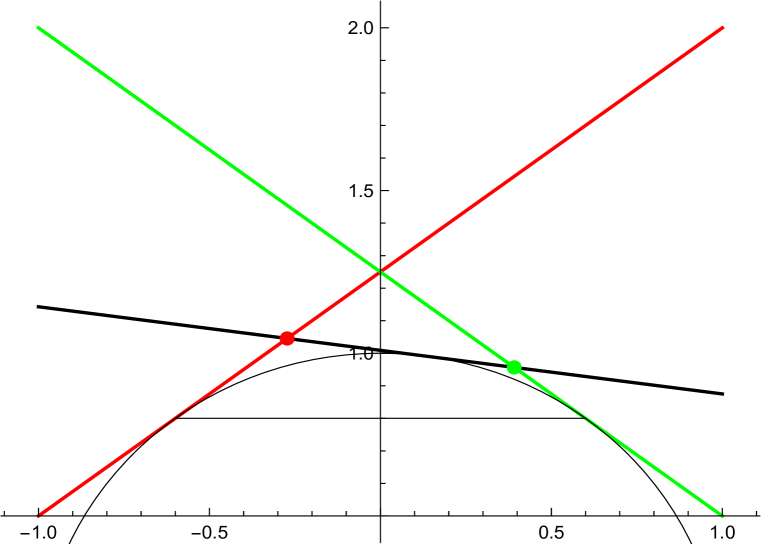
Figure 3: Diagram for ‘tilting transformation’

A transformation, called a ‘tilting transformation’ is now defined. In this context refer to Figure 3. A side is ‘tilted’, its tangent contact point moved, so that it becomes parallel to the line joining the contact points of adjacent sides. All tangent points except one remain fixed. Suppose the initial configuration is as shown in the figure. The red and green tangent lines remain fixed, but suppose the tangent point of the black side is considered movable. The fixed tangent points either side of the movable one are at

$$\zeta_{-}=(-X,h),\qquad\zeta_{+}=(X,h).$$

The coordinates of the movable tangent point might be taken as

$$\zeta=\rho\left(\frac{1-t^{2}}{1+t^{2}},\frac{2t}{1+t^{2}}\right)\ \ {\rm\ and\ w.l.o.g.\ }\rho=1.$$

The area $A(t)$ of the quadrilateral obtained from intersecting the tangential $n$-gon with the half-space $\{y>h\}$ can be found, as can the length $L(t)$ of the three line segments in the upper part of its perimeter. Finding the formulae for $A(t)$ and $L(t)$ is not too onerous, with one check being that $2A(t)-L(t)$ is independent of $t$. Both $A(t)$ and $L(t)$ are minimized at $t=1$ which has the topmost (black) tangent line parallel to $y=h$ and the two consecutive angles of the tangential $n$-gon equal.

Repeated application of the tilting transformation, for varying sides, will, in the limit, get one to a tangential $n$-gon with all angles equal. If a tangential $n$-gon has all angles equal it is regular. Thus, amongst all tangential $n$-gons with radius $\rho$, that which has the smallest area (and perimeter $L=2A/\rho$) is the regular $n$-gon.

Similarly, amongst all tangential $n$-gons with radius $\rho$, that which has the smallest $d_{O}$ is the regular $n$-gon.

The ‘tilting transformation’ is easy to visualize geometrically. Less obvious is that at fixed $\rho$ one can reduce $A$, $L$, $i_{2}$, $i_{4}$, $d_{O}$ by averaging any two angles (not necessarily adjacent angles as above). The reduction of $L$ is a consequence of the convexity of the $\cot$ function on $(0,\pi/2)$, the quantities $T_{k}$ defined in Part IIa equation 6.8) and the representation of $L$ as the sum of the $T_{k}$. The other quantities $i_{2}$, etc. are treated similarly. More details are given in §16.1.

12.7 Circum-$n$-gons to circum-$m$-gons, $m\leq{n}$

Let $\Omega$ be a tangential polygon with inradius $\rho_{0}$ and with the maximum distance of the boundary to the origin $d_{O}$. Then, for any ball $B$ centred at the origin, the convex hull ${\rm conv}(B\cup{\Omega})$ is a tangential polygon.
ToDo. Prove this and investigate the behaviour of $L/\rho$ as the radius of $B$ increases from $\rho_{0}$ to $d_{O}$.

12.8 Minkowski sums

The Minkowski sum of convex polygons is a convex polygon.

The Minkowski sum of two line segments is a parallelogram.
The Minkowski sum of two triangles is a hexagon (usually not tangential).
Any convex polygon is the Minkowski sum of triangles and line segments. A reference for this (which I have yet to check) is page 177 of
I. M. Yaglom, V. G. Boltyanskii, (1961) Convex Figures, New York: Holt, Rinehart and Winston.
This leads on to the following.

Questions. (i) Is any convex hexagon the Minkowski sum of 2 triangles?
(ii) Is, for $n\geq{6}$, any convex $n$-gon with origin at the centroid the Minkowski sum of a small number (perhaps just 2) of tangential $m$-gons (with $m\leq{n/2}$), now (unlike everywhere else in this document) all with centroid at the origin?
A positive answer to a question like this might suggest, from properties established for all tangential $m$-gons, corresponding properties for convex $n$-gons. And if this were to be the case, one can imagine establishing some domain-functional property for tangential $n$-gons and then getting something from the concavity of the domain-functional under Minkowski sum.

12.9 Rearrangements???

For the purely geometric functionals $A$, $L$, $i_{2}$, $i_{4}$, $Q_{0-}$, $d_{O}$ studied in this document rearrangements might not be needed. For functionals, like conformal inradius, transfinite diameter, torsional rigidity, fundamental frequency – functionals involving integrals of gradient squared, etc. – rearrangements are an appropriate tool. [69] used Steiner symmetrization to establish, for triangles and quadrilaterals, that, at given area, the regular $n$-gon optimizes. These are equilateral triangle and square respectively. However, Steiner symmtrizing polygons with more vertices typically increases the number of vertices. [83, 82, 84] manage to use some sort of rearrangement preserving the number of vertices of a convex $n$-gon. Dissymetrization?
ToDo. Try to understand this. See also [4]

Polarizations seem to be building blocks for the rearrangements with which I am more familiar, namely those used in [69]. Polarizations, alone, are not likely to be a tool for rearranging tangential polygons. The following guesses and questions began with drawing sketches.

• The polarization of a triangle about an angle bisector just reflects the triangle.

• Can anything beyond the incircle staying fixed be said about the polarization of a triangle about any line through the incentre? Similar question for any tangential polygon $\Omega$ about any line through the incentre? Non-convex circumgons?

[82]
(i) presents results of the kind that regular $n$-gons optimize over all $n$-gons with the same area;
(ii) that tangential polygons are used (see Part III §22).
A process called ‘dissymetrization’ gets used. This, and polarization, get a mention in [84].

12.10 Spaces of polygons?

See [28].

13 Construction of tangential polygons

With just a few exceptions (on 1-cap, etc.) to date our computations have been for tangential $n$-gons.

Our first method provided data for actually drawing up the polygon and required an initial specification of the inradius. After this prescribe $n$ (which in our computations so far just $n\leq{6}$). Then choose $n$ increasing values of $\theta_{k}$ in $(-\pi,\pi)$ with the maximum difference of consecutive $\theta_{k}$ less than $\pi$. This yields $\exp(\theta_{k})$ on the unit circle as tangent points. (The restriction on the separation of the $\theta_{k}$ is in order that a convex polygon is constructed.) From each pair of consecutive tangent points, find the point of intersection of the tangent lines. These give the vertices of the tangential polygon and there are standard formulae for perimeter $L$, area $A$, in terms of the coordinates but it is easier to note that with the tangent lengths one can find the $T_{k}$ and use these to find $L$, $i_{2}$, $i_{4}$, etc.

If one doesn’t need to draw the polygon and is interested in functionals that stay constant under change of scale, e.g. $L/\rho$, one can use the $T_{k}$ as defined in Part IIa equation (6.8). The tangent lengths are given by $\eta_{k}=\rho\,T_{k}$. Simple formulae to find the other functionals $L$, $i_{2}$, $i_{4}$ are given Part IIa §6.1, and another $d_{O}$ in §19.

We start from result given at the beginning of §12:
Existence Theorem.Given a convex $n$-gon, and hence its sequence of angles, all less than $\pi$, then one can define a tangential $n$-gon whose incentre is at the origin, with the same sequence of angles.
Clearly once one has one, one can rescale by any factor preserving the properties.

Corollary. Given a set $S$ of $n$-numbers $0<\alpha_{k}<\pi$ summing to $(n-2)\pi$, then the different tangential $n$-gons arising from the different permutations of $S$ all have the same values for

$$\frac{L}{\rho},\ \ \frac{i_{2}}{\rho^{3}},\ \ \frac{i_{4}}{\rho^{5}},\ \ \frac{d_{O}}{\rho}.$$

In any event, for many calculations later in this part, one can start directly with the tangent lengths, or with the $\alpha_{k}$ or with the $T_{k}$: it is not always necessary to calculate the vertex coordinates.

In some contexts moving between tangential $n$-gons by permuting angles may lose properties. In particular, permuting angles of a bicentric $n$-gon will, in general result in a tangential $n$-gon which is not bicentric. (The simplest example would be any bicentric quadrilateral with 4 different angles. Permuting the angles must lose the property that the sum of opposite angles is $\pi$.)

While $d_{O}$, the distance from the incentre origin to a vertex, doesn’t need the vertex coordinates and and is invariant, at fixed $\rho$ under permutations of the angles, this may not be the case for the circumradius $R$.

14 Duality

Denote the inner product for plane vectors with a dot. Define polar-reciprocation $\cal P$ of a point $x$ by

$${\cal P}(x)=\{z\ |\ z\cdot{x}=1\}.$$

$\cal P$ takes a point to a line. (This differs from the most common definition of polar in convex geometry in which one has $z\cdot{x}\leq{1}$ so points map to half-planes.) Next continue the definition. Let $D$ be a set in the plane. Define ${\cal P}(D)$ by

$${\cal P}(D)=\{z\ |\ z\cdot{x}=1\ \forall x\in{D}\}.$$

$\cal P$ takes the unit circle to itself. $\cal P$ takes lines (not through the origin) to points: in particular $\cal P$ takes a line tangent to the unit circle to its point of tangency with the unit circle.

See
https://en.wikipedia.org/wiki/Pole_and_polar
https://en.wikipedia.org/wiki/Dual_polygon

Thus the boundary lines of a tangential polygon map to the vertices of a cyclic polygon and vice-versa.

‘Vertex-side’ duality, adapted from wikipedia

As an example of the side-angle duality of polygons we compare properties of the cyclic and tangential polygons, especially quadrilaterals.

Cyclic $n$-gon	Tangential $n$-gon
Circumscribed circle	Inscribed circle
Perpendicular bisectors of the sides are	Angle bisectors are
concurrent at the circumcentre	concurrent at the incentre
$n$ even: The sums of the two pairs	$n$ even: The sums of the two pairs
of opposite/alternate angles	of opposite/alternate sides
are equal	are equal

For a cyclic $2m$-gon the sum of the alternate angles is $(m-1)\pi$. We remark that for quadrilaterals, $m=4$ $n=2$ the converse is true but it is false for $n\geq{3}$. The same is true for tangential $2m$-gons: for $m\geq{3}$ being ‘2-special’ is necessary but not sufficient for a $2m$-gon to be tangential.

$n=6$, $m=3$. Brianchon’s theorem states that the three main diagonals of a tangential hexagon are concurrent.
The polar reciprocal and projective dual of the conics version of Brianchon’s theorem give Pascal’s theorem.

Duality is evident again when comparing an isosceles trapezoid to a kite.

Isosceles trapezoid	Kite
Two pairs of equal adjacent angles	Two pairs of equal adjacent sides
One pair of equal opposite sides	One pair of equal opposite angles
An axis of symmetry through	An axis of symmetry through
one pair of opposite sides	one pair of opposite angles
Circumscribed circle	Inscribed circle

Let $P(n)$ be an ordered list of $n$ points $\zeta_{k}$ on a circle, $P(n+1)=P(n)\cup\{\zeta_{n+1}\}$ with $\zeta_{n+1}$ after $\zeta_{n}$ and before $\zeta_{1}$.
Let $TP(P(n))$ be the tangential $n$-gon with the points of $P(n)$ its tangent points.
Let $CP(P(n))$ be the cyclic $n$-gon with the points of $P(n)$ its vertices. The first entry in the table below indicates how areas change on introducing the additional point on the circle.

$|TP(P(n+1))|\leq|TP(P(n))|$	$|CP(P(n+1))|\geq|CP(P(n))|$
A tangential $2m$-gon has all sides equal iff	A cyclic $2m$-gon has all angles equal iff
the alternate angles are equal.	the two sets of alternate sides are equal.
Equilateral tangential for $n=2m$ even	Equiangular cyclic for $n=2m$ even
Opposite angles equal if $n/2$ is even	Opposite sides equal if $n/2$ is even

See [90].

14.1 Tangential and cyclic polygons, continued

The set of all convex sets is a lattice under operations of intersection, $\Omega_{1}\cap\Omega_{2}$, and convex-hull of union, ${\rm conv}(\Omega_{1}\cup\Omega_{2})$.
The set of tangential polygons with incentre at the origin and given inradius $\rho$ is closed under intersection.
The set of cyclic polygons with circumcentre at the origin and given circumradius $R_{V}$ is closed under convex-hull-union. (A cyclic polygon is the convex hull of its extreme points all of which lie on the circle radius $R_{V}$.)
In the case of $n$-gons the numbers of vertices can increase.

Let the coordinates of the vertices of a convex $n$-gon be $(x_{k},y_{k})$ with the vertices traversed in order (and vertex 1 identified with vertex $n+1$).
The polygon is cyclic with circumcentre O and circumradius 1 if the distance of every vertex from O is 1:

$$x_{k}^{2}+y_{k}^{2}=1\qquad\forall k.$$

The polygon is tangential with incentre O and inradius 1 if the distance of every side from O is 1:

$$(x_{k+1}-x_{k})^{2}+(y_{k+1}-y_{k})^{2}=(x_{k+1}y_{k}-y_{k+1}x_{k})^{2}\qquad\forall k.$$

The tangency point on each line, the closest point to O, is

$$x_{t}=\frac{y_{k+1}-y_{k}}{x_{k}\,y_{k+1}-y_{k}\,x_{k+1}},\qquad y_{t}=\frac{x_{k+1}-x_{k}}{x_{k}\,y_{k+1}-y_{k}\,x_{k+1}}.$$

In establishing, by Steiner symmetrisation, isoperimetric properties of $n$-gons, for $n=3$ and $n=4$, sequences of polygons which alternate between tangential and cyclic occur. Here is a quote from [69]:

Of all quadrilaterals with a given $A$, the square has the smallest $L$, $I_{c}$ (polar moment of inertia about the centroid), $\overline{r}$, …but the largest $\dot{r}$ and $Q_{0}$. ……it is sufficient to indicate a sequence of symmetrizations which transform, ultimately, a given quadrilateral into a square. Symmetrizing a given quadrilateral with respect to a perpendicular to one of ·its diagonals, we change it into a quadrilateral having a diagonal as axis of symmetry. Symmetrizing this new quadrilateral with respect to a perpendicular to its axis of symmetry, we change it into a rhombus. Symmetrizing the rhombus with respect to a perpendicular to one of its sides, we change it into a rectangle. Symmetrizing the rectangle with respect to a perpendicular to one of its diagonals, we obtain another rhombus. Repeating the last two steps in succession, we obtain an infinite sequence in which rhombi alternate with rectangles.

Rhombi are tangential polygons (with equal sides):
rectangles are cyclic (with equal angles).

Steiner symmetrization is not applicable to showing that regular $n-gons$ optimize when $n\geq{5}$. If one (initially at least) focuses on geometric quantities like

$$\frac{A}{L^{2}},\ \frac{i_{2}}{L^{3}},\ \frac{i_{4}}{L^{4}},\qquad{\rm and\ }\ \frac{Q_{0-}}{A^{2}},$$

it may be possible to devise other transformations between $n$-gons
which alternate between tangential and cyclic,
which change functionals like those immediately above monotonically and
which converge to the regular $n$-gon.

15 Miscellaneous properties of tangential polygons

15.1 Circulant matrices and tangential $n$-gons

This subsection treats questions like the following:
Given a set of $n$ of positive side lengths $(s_{j})$ how can we recognize if there could be a tangential polygon with these side lengths?

We begin with a connection between tangential polygons and circulant matrices presented near the beginning of the wikipedia page on tangential polygons.

Let $P$ and $M=I+P$ be the $n\times{n}$ circulant matrices as follows. $P$ is the $n\times{n}$ cyclic permutation:

$$P=\begin{pmatrix}0&1&0&\cdots&0\\ 0&0&1&\cdots&0\\ \vdots&\vdots&\vdots&\ddots&\vdots\\ 1&0&0&\cdots&0\end{pmatrix}$$

The matrix $\frac{1}{2}M$ is doubly stochastic.

The wikipedia page states:

There exists a tangential polygon of $n$ sequential sides $s_{1},\ldots,s_{n}$ if and only if the system of equations

$$M{\mathbf{\eta}}={\mathbf{s}},$$ (15.1)

has a solution $(\eta_{1},\dots,\eta_{n})$ in positive reals. If such a solution exists, then $(\eta_{1},\dots,\eta_{n})$ are the tangent lengths of the polygon (the lengths from the vertices to the points where the incircle is tangent to the sides).

Once one has the $\eta$ and $\rho$ the angles $\alpha_{k}$ are determined from

$$\eta_{k}(=\eta_{k-})=\rho T_{k}\qquad{\rm where\ \ }T_{k}=\frac{1}{\tan(\frac{\alpha_{k}}{2})}.$$

See PartIIa, equation (6.8). That the sum of the $\alpha_{k}$ is $(n-2)\pi$ leads to one further equation which we record, as an aside, in the next subsubsection.

15.1.1 Some relations between the $T_{k}$

As before, consider $n$-gons and denote the angle at vertex $k$ by $\alpha_{k}$, with $k$ increasing as one goes around the convex $n$-gon in counterclockwise direction. The sum over all the $\alpha_{k}$ is $(n-2)\pi$.

Fix the inradius $\rho$ as 1. Suppose the points of tangency of the tangential $n$-gon are $\zeta_{j}=\exp(i\phi_{j})$. Again $j$ increases as one goes around the convex $n$-gon in counterclockwise direction. The angle at O formed by the lines $O\zeta_{j}$ and $O\zeta_{j+1}$ is $\phi_{j+1}-\phi_{j}$.

Then, with

$$T_{k}=\frac{1}{\tan\frac{\alpha_{k}}{2}}=\tan(\frac{\pi-\alpha_{k}}{2}),$$ (15.2)

$T_{k}>0$ since the polygon is convex. Since we know the sum of $\alpha_{k}/2$:

$$\sum_{k=1}^{n}\frac{\alpha_{k}}{2}=\sum_{k=1}^{n}{\rm arccot}(T_{k})=(n-2)\frac{\pi}{2}.$$ (15.3)

Some, but not all, the information in this can be expressed in equations involving just rational functions of the $T_{k}$, i.e. without the transcendental arccot function. We denote the elementary symmetric polynomial of degree $k$ by

$${\rm SymmetricPolynomial}(k,\ldots),$$

and define

$$e_{k}={\rm SymmetricPolynomial}(k,[\frac{1}{T_{1}},\frac{1}{T_{2}},\ldots,\frac{1}{T_{n}}]).$$

For tangential $n$-gons, we first treat $n$ odd, then $n$ even.
When $n$ is odd $\cos((n-2)\pi/2)=0$ so the cosine of the sum of all the $\alpha_{k}/2$ is $0$ we have

$$e_{0}-e_{2}+e_{4}-e_{6}\dots=0.$$ (15.4)

When $n$ is even $\sin((n-2)\pi/2)=0$ so the sine of the sum of all the $\alpha_{k}/2$ is $0$ we have

$$e_{1}-e_{3}+e_{5}-e_{7}\dots=0.$$ (15.5)

We will need the formulae for perimeter, i.e. $L=i_{0}$, for $i_{2}$ and for $i_{4}$ as given in Part IIa §6.1 namely equations (6.9), (6.10) and (6.11).

15.1.2 Examples at $n=3$ or $4$

For a triangle $A={\sqrt{\frac{L}{2}(\frac{L}{2}-a)(\frac{L}{2}-b)(\frac{L}{2}-c)}}$ and since $L=2\sum\eta_{k}$

$\mathrm{tang3gon}:A=\sqrt{({\eta }_1+{\eta }_2+{\eta }_3){\eta }_1{\eta }_2{\eta }_3}.$

For a tangential quadrilateral wikipedia gives

$\mathrm{tang4gon}:A=\sqrt{({\eta }_1+{\eta }_2+{\eta }_3+{\eta }_4)({\eta }_1{\eta }_2{\eta }_3+{\eta }_2{\eta }_3{\eta }_4+{\eta }_3{\eta }_4{\eta }_1+{\eta }_4{\eta }_1{\eta }_2)}.$

Figure 4: From wikipedia. Brianchon’s Theorem. Diagonals of a tangential hexagon are concurrent.

15.1.3 Non-negative solution for $\mathbf{\eta}$ given $\mathbf{s}$?

Return now to the linear equations (15.1). Denote the dependence of $M$ on $n$ by writing $M(n)$. There is very different behaviour when $n$ is odd than when $n$ is even as, for example,

$${\rm det}(M(n))=1-(-1)^{n}.$$

Thus $M(n)$ is invertible when $n$ is odd, but not when $n$ is even. There being many questions I have been, as yet, unable to answer, and as properties of $M(n)$ might ultimately be useful, I have collected several properties of $M(n)$ here, but not found uses for some of them yet. Let ${\mathbf{e}}$ be the vector all of whose entries are 1. Then, for all $n$,

$$M(n)\,{\mathbf{e}}=2\,{\mathbf{e}}.$$

Geometrically this corresponds to a regular $n$-gon with side 2 and tangent lengths 1. The eigenvalues of $P$ are the roots of unity, and the eigenvalues of $M$ require us just add 1 to these. The eigenvectors are, of course, the same.

$${\rm CharacteristicPolynomial}(M(n),\lambda)=-(-1)^{n}(1-(\lambda-1)^{n}).$$

The transpose $M^{T}(n)$ has exactly the same properties as described for $M(n)$ in the preceding paragraph. If one ignores the nonnegativity requirement, clearly there is, for any rhs $\mathbf{s}$ a unique ‘solution’ to the linear equations when $n$ is odd. When $n$ is even, there is only a ‘solution’ when the rhs is orthogonal to the nullspace of $M^{T}(n)$, i.e only when

$$\sum_{k\ {\rm odd}}s_{k}=\sum_{k\ {\rm even}}s_{k},$$ (15.6)

and, also, ‘solutions’ are not unique.

$M(n)$ is normal, commutes with its transpose. As $M\,M^{T}$ is symmetric and Toeplitz it is centrosymmetric.

A persymmetric matrix is a square matrix which is symmetric with respect to the northeast-to-southwest diagonal. $M(n)$ is persymmetric and, as such, satisfies

$$M(n)\,J=J\,M^{T}(n),\qquad{\rm where\ }J\ {\rm is\ the\ exchange\ matrix}.$$

$J$ is the matrix with 1s on its northeast-to-southwest diagonal and 0s elsewhere.

Define next

$$M_{i}(n)=(I(n)+\sum_{k=1}^{n-1}(-1)^{k}P(n)^{k})/2.$$

We have

$$M(n)\,M_{i}(n)=\frac{1-(-1)^{n}}{2}I(n).$$

For $n$ odd $M_{i}(n)$ is the inverse of $M(n)$. Also (via Cayley-Hamilton Theorem)

$$\sum_{k=1}^{n}(-1)^{k}{n\choose k}M(n)^{k}=-(1-(-1)^{n})\,I(n).$$

The obvious next question is ‘what conditions on the sides ensure there is a nonnegative solution for $\mathbf{\eta}$’?

Farkas Lemma. Exactly one of the following two assertions is true:
1.There exists an ${\mathbf{\eta}}\in{\mathbb{R}^{n}}$ such that $M{\mathbf{\eta}}={\mathbf{s}}$ and ${\mathbf{\eta}}\geq 0$.
2. There exists a $\mathbf{y}\in\mathbb{R}^{n}$ such that $\mathbf{M}^{\mathsf{T}}\mathbf{y}\geq 0$ and $\mathbf{s}^{\mathsf{T}}\mathbf{y}<0$.
We have yet to devise a good use for this lemma but suspect it will be relevant to conditions for general $n\geq{3}$.

Here we do not attempt to find the conditions for general $n$. We will attempt to find necessary and sufficient conditions on $\mathbf{s}$ for the existence of nonnegative $\mathbf{\eta}$, separately, for each of $n=3$, 4, 5 and 6.

Triangles. When $n=3$,

$$M(3)^{-1}=\frac{1}{2}\left(\begin{array}[]{ccc}1&-1&1\\ 1&1&-1\\ -1&1&1\\ \end{array}\right),$$

so one has nonnegative solutions for $\eta$ iff the nonnegative $s$ are such that the sum of any two is greater than (or equal to) the remaining side’s length. This accords with the fact that any triangle is tangential (indeed bicentric).

Tangential pentagons. When $n=5$,

$$M(5)^{-1}=\frac{1}{2}\left(\begin{array}[]{ccccc}1&-1&1&-1&1\\ 1&1&-1&1&-1\\ -1&1&1&-1&1\\ 1&-1&1&1&-1\\ -1&1&-1&1&1\\ \end{array}\right).$$

Consider triples of sides in which just one pair of sides are adjacent. There are five such triples. There are nonnegative solutions for $\eta$ iff the nonnegative $\mathbf{s}$ are such that for any of these five triples the sum of those in the triple is greater than (or equal to) the sum of the remaining two sides’ lengths.

Let $n=2m$ for $m\geq{2}$. Define

$${\mathbf{nv}}=\left(\ (-1)^{k}\ \right),$$

which is a basis for the nullspace of $M(n)$ (and also of $M^{T}(n)$). Suppose $\mathbf{s}$ satisfies equation (15.6) so ‘solutions’, albeit without the nonnegativity condition imposed, exist. These solutions are

$${\mathbf{\eta}}_{\rm gen}={\rm PseudoInverse}(M(n))\,{\mathbf{s}}+c\,{\mathbf{nv}},$$ (15.7)

but it remains to investigate the restrictions on $\mathbf{s}$ and $c$ needed so that amongst the ${\mathbf{\eta}}_{\rm gen}$ there is at least one with ${\mathbf{\eta}}\geq{0}$. In this document we will attempt this only for $n=4$ and $n=6$. Before that, however, we consider $n=2m$ in general. By standard properties

$$M(n)\,{\rm PseudoInverse}(M(n))\,M(n)=M(n).$$

Using the fact that when $n=2m$ the matrix $M(n)$ has the simple block structure

$$M(n)=\begin{pmatrix}U&L\\ L&U\end{pmatrix},$$

it is easy to find $A$ and $B$ so that

$${\rm PseudoInverse}(M(n)=\begin{pmatrix}A&B\\ B&A\end{pmatrix}.$$

The matrix $L$ has just one 1 in the bottom left corner and $U=M(m)-L$. We have

$$A = \frac{1}{2}({\rm PseudoInverse}(U+L)+{\rm PseudoInverse}(U-L)),$$

$$B = \frac{1}{2}({\rm PseudoInverse}(U+L)-{\rm PseudoInverse}(U-L)).$$

We also have $L\,U\,L$ is the zero matrix, and $L\,U^{-1}\,L=-L$.

Tangential quadrilaterals. It is already known that no further restriction beyond

$$s_{1}+s_{3}=\frac{L}{2}=s_{2}+s_{4}$$

is needed to ensure that the quadrilateral is tangential. So it remains just an exercise to show that the system of equations

$$M(4){\mathbf{\eta}}=\begin{pmatrix}s_{1}\\ s_{2}\\ \frac{L}{2}-s_{1}\\ \frac{L}{2}-s_{2}\end{pmatrix}$$

has, for all $0<s_{1}<L/2$ and $0<s_{2}<L/2$ a positive $\eta$ solution. When $n=4$,

$${\rm PseudoInverse}(M(4))=\frac{1}{8}\left(\begin{array}[]{cccc}3&-1&-1&3\\ 3&3&-1&-1\\ -1&3&3&-1\\ -1&-1&3&3\\ \end{array}\right).$$

There is no loss of generality in setting $L=2$ and considering $1/2\leq{s_{1}}<1$ and $1/2\leq{s_{2}}<s_{1}$. If we try the formula (15.7) we are led to consider the function $\phi$

$$\phi(s_{1},s_{2},c)={\rm min}(1+2s_{1}-2s_{2}-c,-1+2s_{1}+2s_{2}+c,1-2s_{1}+2s_{2}-c,3-2s_{1}-2s_{2}+c),$$

over the triangle in $(s_{1},s_{2})$ space defined in the preceding sentence. Considering the final entry in the min defining $\phi$, we have $\phi(s,s,0)<0$ for $3/4<s<1$, so we need to choose $c$ (which can depend on $\mathbf{s}$) appropriately. We find, over the triangle in $(s_{1},s_{2}$-space $\phi(s_{1},s_{2},2s_{1}+2s_{2}-3)=0$, i.e. the last entry is zero but the other 3 entries are nonnegative. Except for a positive multiple, the other 3 entries (first 3) are

$$1-s_{2},-1+s_{1}+s_{2},1-s_{1}.$$

Tangential hexagons. Unlike the situation with $n=4$ extra conditions on the sides are needed. The corresponding problem for cyclic hexagons is mentioned in  [91] (and the same author has other papers involving tangential and cyclic hexagons, [88], [90]).

After writing the above, I found [15] gives the following.

Theorem.There will be a tangential hexagon with given side lengths $s_{1},s_{2},...,s_{6}$ if and only if the equality

$$s_{1}+s_{3}+s_{5}=s_{2}+s_{4}+s_{6},$$

and the following nine inequalities are satisfied:

$$s_{1}>0,s_{2}>0,...,s_{6}>0,$$

$$s_{1}-s_{2}+s_{3} > 0,$$

$$s_{3}-s_{4}+s_{5} > 0,$$

$$s_{5}-s_{6}+s_{1} > 0.$$

In words, the length of any side is less than the sum of the lengths of the adjacent sides.

[15] also gives the conditions on $\mathbf{s}$ for an octagon to be tangential. When $n=6$,

$${\rm PseudoInverse}(M(6))=\frac{1}{12}\left(\begin{array}[]{cccccc}5&-3&1&1&-3&5\\ 5&5&-3&1&1&-3\\ -3&5&5&-3&1&1\\ 1&-3&5&5&-3&1\\ 1&1&-3&5&5&-3\\ -3&1&1&-3&5&5\\ \end{array}\right).$$

(On looking at the corresponding outputs for large $n=2m$ one finds that $2n$ times ${\rm PseudoInverse}(M(n))$ has entries $\pm$ odd integers less than $n$. And, as noted before, there is a block matrix structure too.)

ToDo. Check out that the conditions on $\mathbf{s}$ given in [15] are necessary and sufficient to ensure that $\eta$ is nonnegative.

15.2 Geometric isoperimetric inequalities

Lets begin with the first, historic, instance of an isoperimetric inequality in which regular $n$-gon optimizes over all $n$-gons. The following argument is from geometers in ancient Greece, perhaps around 200BC.

L-A Isoperimetric Result. Amongst convex $n$-gons with given perimeter, that which has the largest area is the regular $n$-gon.

Start with a convex $n$-gon, $\Omega_{0}$. Suppose $P_{i-1}$, $P_{i}$, $P_{i+1}$ are consecutive vertices. (i) show that among all isoperimetric triangles with the same base the isosceles triangles has maximum area. Thus by changing $\Omega_{0}$ moving point $P_{i}$ to $P_{i}^{\prime}$ with $P_{i-1}$, $P_{i}^{\prime}$, $P_{i+1}$ isosceles, the area of the changed polygon is increased. Apply this process to all triples of consecutive vertices. By iteration, one finds that the optimal polygon must be equilateral: call it $\Omega_{1}$.
(ii) show that if the polygon $\Omega_{1}$ is not equiangular, its area may be increased by redistributing perimeter from a pointy to a blunt angle until the two angles are the same.

An alternative to (ii) is to use that Among all $n$-gons with given side lengths, the cyclic $n$-gon has the largest area. And a cyclic $n$-gon with equal sides is regular.

(For this and related isoperimetric inequalities see [3]. See also [90] concerning equiangular and equilateral considerations.)

By a $\cal D$ we shall mean some domain functionals, and we are interested in pairs of these for which one has a result of the form
For tangential $n$-gons with fixed ${\cal D}_{1}$ the regular $n$-gon $<$maximizes$|$minimizes$>$ ${\cal D}_{2}$
Table 4 below presents some:

${\cal D}_{1}$		${\cal D}_{2}$	Remark
area	min	perimeter
area	max	inradius	$A=\rho L/2$
inradius	min	perimeter	Jensen inquality
inradius	min	area	”
inradius	min	$i_{2}=\frac{16\Sigma_{\infty}}{\rho}$	”
inradius	min	$i_{4}$	”

Table 4: Tangential $n$-gons

The Jensen inequality/convexity concerns convex functions $\phi$ on some interval $I$, and that

$${\rm with}\ x_{i}\in{I}\ {\rm and}\ \sum a_{i}=1\ {\rm with}a_{i}\geq{0}\ ,\ \phi(\sum a_{i}x_{i})\leq\sum a_{i}\phi(x_{i}).$$

The inequality is reversed for concave $\phi$. By using the formula for the length for a $n$-gon given at equation (6.9) and the convexity of $\cot(\cdot/2)$ on $(0,\pi)$ we have the first entry of the following.

• We use $\cot(\alpha/2)$ convex for $\alpha\in(0,\pi)$ and (6.9). We have

  $$\frac{L}{2\rho n}=\sum\frac{1}{n}\cot(\frac{\alpha_{k}}{2})\geq\cot\left(\sum\frac{1}{n}\frac{\alpha_{k}}{2}\right)=\cot(\frac{(n-2)\pi}{2n})\frac{L_{n}}{2\rho n},$$

  where $L_{n}$ is the perimeter of the regular $n$-gon with inradius $\rho$. This establishes the entry in the table corresponding to fixed $\rho$, mimimizing the perimeter (and since $A=\rho\,L/2$ also minimiing $A$).

• Using that

  $$\cot(\frac{\alpha}{2})+\frac{\cot(\frac{\alpha}{2})^{3}}{3}\ \ {\rm convex\ for\ }\alpha\in(0,\pi),$$

  and the formula (6.10) the Jensen inequality approach above gives that, at fixed $\rho$, $i_{2}$ is minimized by the regular polygon with the same number of sides.

• Starting from formula (6.11), the result on $i_{4}$ follows in the same way.

For cyclic $n$-gons with fixed ${\cal D}_{1}$ the regular $n$-gon $<$maximizes$|$minimizes$>$ ${\cal D}_{2}$
Table 5 below presents some:

${\cal D}_{1}$		${\cal D}_{2}$	Remark
area	min	perimeter
area	max	inradius
circumradius	max	perimeter	Jensen inquality
circumradius	max	area	”

Table 5: Cyclic polygons

There is a huge literature even restricting to convex sets.
https://math.stackexchange.com/questions/749528/isoperimetric-inequality-isodiametric-inequality-hyperplane-conjecture-what

Also the ‘stability’ of the isoperimetric inequalities is studied in many different ways sometimes involving ‘isoperimetric deficit’, sometimes ‘Fraenkel asymmetry’.

If $L$ is the perimeter of a convex polygon $\Omega$, $A$ its area, $\rho$ the inradius, and $s$ the length of any chord through the centre of a largest inscribed circle, then

$$L^{2}-4\pi A\geq\frac{\pi^{2}}{4}(s-2\rho)^{2}.$$

This is a sharpened isoperimetric inequality for convex polygons.
H. Hadwiger, Comment. Math. Helv. 16 (1944),305-309.
Tangential polygons can be regarded as limits of tangential $n$-gons, so the inequality applies to them and is

$$L(L-2\pi\rho)\geq\frac{\pi^{2}}{4}(s-2\rho)^{2}.$$

In notation as in the list at the beginning of §19,

$$s\geq d_{O}+\rho\qquad{\rm so}\ \ L(L-2\pi\rho)\geq\frac{\pi^{2}}{4}(d_{O}-\rho)^{2}.$$

With, as in §19.5, $x=L/d_{O}$, $y=\rho/d_{O}$,

$$x\,(x-2\pi y)\geq\frac{\pi^{2}}{4}(1-y)^{2},$$

or

$$x=\frac{1}{2}\pi\left(\sqrt{5y^{2}-2y+1}+2y\right).$$

This gives a curve bit left of the upper left 1-cap curve of Figure 12.

There is a considerable literature concerning moments of inertia about the centroid. (There are, of course, situations involving appropriate symmetries when the centroid and incentre will coincide.)
Results. The equilateral triangle minimizes the moment of inertia, among all convex curves with given perimeter.
References include [40], [85], [64]. See also §20.

15.3 Further geometric items

For every convex domain

$$\pi\rho+\frac{|\Omega|}{\rho}\leq|\partial\Omega|\leq 2\,\frac{|\Omega|}{\rho}.$$

See [20] equation (8). For tangential polygons the right hand side is an equality and the left-hand side is just $L\geq{2}\pi\rho$.
There may be some use for Bonnesen inequalities, see [66], and stronger forms for tangential polygons.

Repeat here, for the third time(!), the existence statement of §12 and of §13. Let there be given a convex polygon, and hence its sequence of angles, all less than $\pi$. Then one can define a tangential polygon with the same sequence of angles and the same area.

A tangential polygon has a larger area than any other convex polygon with the same perimeter and the same interior angles in the same sequence. (See [2, 54, 93].)
Amongst all convex polygons with the same area and with the same interior angles in the same sequence
(i) those which have the smallest perimeter are tangential polygons, and
(ii) those which have the largest inradius are tangential polygons.

Amongst all tangential quadrilaterals with a given sequence of side lengths, that which maximizes the area is bicentric.
One starting point is the more general result.
Amongst all quadrilaterals with given side lengths, that which has maximum area is cyclic.
(Proof: Use Bretschneider’s formula.)
(A very easy special case is that the area of a kite with given sides is maximized by the right kite.)

There may be generalization to $2m$-gons, in particular hexagons.
https://mathworld.wolfram.com/CyclicHexagon.html
gives area in terms of sides.

Theorem. For any quadrilateral with given edge lengths, there is a cyclic quadrilateral with the same edge lengths.

Theorem. The cyclic quadrilateral has the largest area of all quadrilaterals with sides of the same length.

15.4 Cheeger constant

For tangential polygons $\Omega$, the Cheeger constant is

$$h_{\Omega}=\frac{|\partial\Omega|+\sqrt{4\pi|\Omega|}}{|2\Omega|}.$$

Clearly, at fixed area, since perimeter is minimized by the regular $n$-gon, the regular $n$-gon minimizes $h_{\Omega}$ over tangential $n$-gons with given area. Much more has been established.

Among all simple polygons with a given area and at most $n$ sides, the regular $n$-gon minimizes the Cheeger constant. (See [16].)

If $\Omega$ is a convex polygon, we denote $\Omega_{*}$ the (unique up to rigid motions) circumscribed polygon which has the same area as $\Omega$ and whose angles are the same as those of $\Omega$, then

$$h(\Omega)\geq h(\Omega_{*}),$$

with equality if and only if $\Omega=\Omega_{*}$ (up to rigid motions).

16 Triangles

Given the area $A$ and the angles $\alpha$, $\beta$ and $\gamma=\pi-\alpha-\beta$ of the triangle, one can determine the inradius and thence, if needed, the sides. We have

$$A=\rho^{2}\left(\cot\frac{\alpha}{2}+\cot\frac{\beta}{2}+\cot\frac{\gamma}{2}\right).$$

The semiperimeter $s=(a+b+c)/2$ is found from

$$s=\frac{A}{\rho}=\rho\,\left(\cot\frac{\alpha}{2}+\cot\frac{\beta}{2}+\cot\frac{\gamma}{2}\right)=\sqrt{A\,\,\left(\cot\frac{\alpha}{2}+\cot\frac{\beta}{2}+\cot\frac{\gamma}{2}\right)}.$$

Now, defining $f$ from

$$\frac{\sin(\alpha)}{a}=\frac{\sin(\beta)}{b}=\frac{\sin(\gamma)}{c}=\frac{1}{f},$$

we have

$$s=\frac{a+b+c}{2}=\frac{f}{2}\,\left(\sin(\alpha)+\sin(\beta)+\sin(\gamma)\right),$$

which determines $f$ and hence all the sides.

Using

$$T_{A}=\frac{1}{\tan(\frac{\alpha}{2})},\quad T_{B}=\frac{1}{\tan(\frac{\beta}{2})},\quad T_{C}=\frac{T_{A}+T_{B}}{T_{A}T_{B}-1},$$

$i_{2}$ and $i_{4}$ can be found from equations (6.10) and (6.11). From these $\Sigma_{\infty}$ and $\Sigma_{1}$ can be found: see Part III §25

With apologies for leaving the write-up in code, all the reasonable results are readily proved for triangles. The code also produces an example of a Blaschke-Santalo diagram, shown in Figure 5, of the kind we will see later for other tangential polygons.

( * An isoperimetric result
Amongst triangles with a given inradius, taken as 1,
that which has the smallest perimeter is the equilateral triangle.
The allowed values of TA>0 and TB>0 are those for which TA*TB>1 *)
TCfn[TA_,TB_]:= (TA+TB)/(TA*TB-1);
Lfn[TA_,TB_]:= TA+TB+TCfn[TA,TB];
(* Lfn ia half the length *)
(* The hessian is positive definite, positive diagonal entries and Det>0
on using TA*TB>1, etc. *)
hess = Map[Simplify, D[tmp, {{TA, TB}, 2}]];
Factor[Det[hess]]
(* Find minimum by checking where gradient is 0  *)
g = Map[Simplify, Grad[Lfn[TA, TB], {TA, TB}]]
Solve[{g[[1]] == 0, g[[2]] == 0}, {TA, TB}]
(* gives (TA,TB) = (Sqrt[3],Sqrt[3]) which is equilateral triangle *)

(* Define also *)
dOfn[TA_,TB_]:= Max[{TA,TB,TCfn[TA,TB]}];
(* One can also show that at given inradius, the triangle which
minimizes the distances from incentre to vertices is equilateral. *)

(* One can also imagine fixing not just the inradius but also dO
and with these TWO constraints finding
(i) the shape with the maximum perimeter,
(ii) the shape with the minimum perimeter.
And find that they come out to be the obvious different sorts of isosceles triangles.
*)


(* Think of A as apex of triangle
Expect to see different behaviour for TA large - small apex angle
to what one gets when TA is small - big apex angle.
Let B the angle I will vary be <= Pi/2 so TB >=1.
Actually TB also gets restricted to be TB >= Max[1,1/TA]
This restiction causes TC>0 *)

(* fix TA, vary TB
 LAfn is a convex function and its first derivative is zero when TB=TC,
 i.e. triangle is isosceles
 So, at fixed rho, the perimeter of a triangle with one angle fixed is
minimized when the triangle is isosceles having TB=TC= (1+Sqrt[1+TA^2])/TA
BCequal = Factor[TCfn[TA, TB] - TB]
Solve[BCequal == 0, TB]
Factor[D[Lfn[TA, TB], TB]/BCequal] (* clearly nonzero *)
Factor[D[Lfn[TA, TB], {TA, 2}]] (* clearly positive *)
Plot[Lfn[TA, (1 + Sqrt[1 + TA^2])/TA], {TA, 0.1, 8}]
(* convex function, minimum at TA=Sqrt[3] *)

tmp = Together[Simplify[D[Lfn[TA,(1 + Sqrt[1 + TA^2])/TA], TA]]]
u = Sqrt[1 + TA^2];
Simplify[tmp - (-2 + u)*(1 + u)^2/(TA^2*u)] (* 0 *)
Simplify[tmp /. TA -> Sqrt[3]]. (* 0 *)

ppu =ParametricPlot[{Lfn[TA,(1+Sqrt[1+TA^2])/TA]/dOfn[TA,(1+Sqrt[1+TA^2])/TA],
 1/dOfn[TA,(1+Sqrt[1+TA^2])/TA]},{TA,0.01,Sqrt[3]},PlotStyle->Red];
ppl =ParametricPlot[{Lfn[TA,(1+Sqrt[1+TA^2])/TA]/dOfn[TA,(1+Sqrt[1+TA^2])/TA],
 1/dOfn[TA,(1+Sqrt[1+TA^2])/TA]},{TA,Sqrt[3],128},PlotStyle->Green];

pairs[AB_] := {Lfn[AB[[1]], AB[[2]]]/dOfn[AB[[1]], AB[[2]]],
   1/dOfn[AB[[1]], AB[[2]]]};
rdm[Npts_] :=
  Module[{k} ,
   Map[pairs,
    Table[{1 + RandomReal[{0, 32}], 1 + RandomReal[{0, 32}]}, {k, 1,
      Npts}]]];
lp = ListPlot[rdm[20000], PlotRange -> All];
rLdOtri = Show[{ppu, ppl, lp}, PlotRange -> All]

Figure 5: Triangles: $x=L/(2d_{O})$, $y=\rho/d_{O}$ with $\rho=1$.

The dots in the figure are from random choices for two of the $T$ values (corresponding to two angles). The large number corresponding to large values of $d_{O}$ is from using a uniform random distribution for the $T$ allowing large values (so thin, or squat, triangles). The red curve is from tall thin isosceles triangles. The green curve is from tall thin isosceles triangles.

16.1 Generalizing, angle-averaging

We have also used Mathematica Minimize on these tasks and it worked well for $n=3$ and $n=4$ and NMinimize for larger $n$. However, having already proved the result using Jensen’s inequality in §15.2 one learnt (very) little from the exercise.

However, one way to learn a little more is to use the convexity of $\cot$ to ‘average two angles’ as remarked upon in the ‘tilting transformation’ treated in §12. We keep $\rho$ fixed, say $\rho=1$. Choose two vertices, with angles $\alpha_{i}$ and $\alpha_{j}$. Let

$$\sigma_{i}=\tan(\frac{\alpha_{i}}{4})\qquad{\rm so\ }\ \ T_{i}=\frac{1-\sigma_{i}^{2}}{2\sigma_{i}}.$$

Then, as

$$\tan(\frac{\alpha_{i}+\alpha_{j}}{4})=\frac{\sigma_{i}+\sigma_{j}}{1-\sigma_{i}\sigma_{j}}).$$

The convexity of the $\cot$ function on $(0,\pi/2)$ is

$$2\cot(\frac{\alpha_{i}+\alpha_{j}}{4}) \leq \cot(\frac{\alpha_{i}}{2})+\cot(\frac{\alpha_{j}}{2}),$$

$$\frac{2(1-\sigma_{i}\sigma_{j})}{\sigma_{i}+\sigma_{j}} \leq T_{i}+T_{j}.$$

From this, and the representation of $L$ as a sum of $T_{k}$, we see that $L$ is reduced by averaging two of the angles.

The same argument works for $i_{2}$ and for $i_{4}$ on using the convexity of $\cot^{3}$ and of $\cot^{5}$.

It is also easy to work out the differences, by how much the quantities $L$, $i_{2}$, etc. decrease.

(* Write T[1]=1/tan(alpha1/2) and T[2] in terms of u1 = tan(alpha1/4) and u2 resp. *)
T[1] = (1-u1^2)/(2*u1);
T[2] = (1-u2^2)/(2*u2);
(* After angle averaging/ optimal tilting when adjacent *)
tAve= (1-u1*u2)/(u1+u2);
Tout[1]= tAve;
Tout[2]= tAve;

Ldifference = Factor[2*(T[1]+T[2]-2*tAve)]
(* (((u1 - u2)^2*(1 - u1*u2))/(u1*u2*(u1 + u2))) *)

i2STfn[TT_]:= (TT+TT^3/3);
i2difference = Factor[2*(i2STfn[T[1]]+i2STfn[T[2]]-2*i2STfn[tAve])]
(* long expression - an obviously positive expression * Ldifference^3 *)

17 Tangential quadrilaterals

We begin with the context:

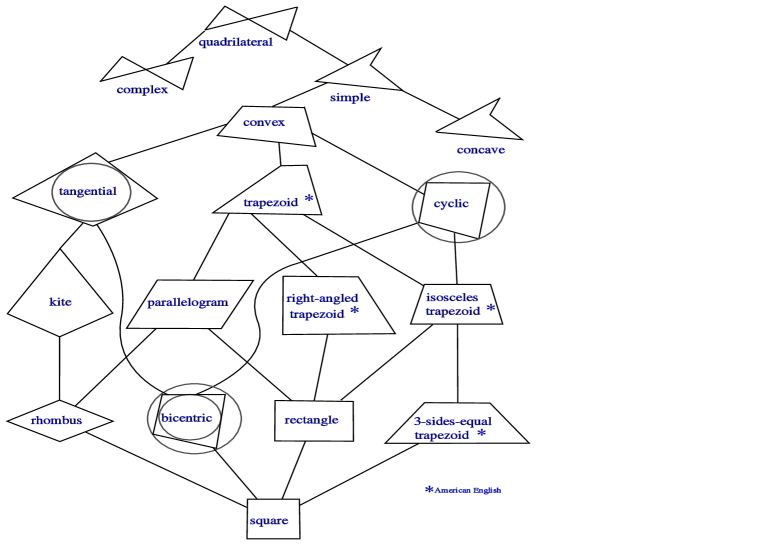
Figure 6: wikipedia, attribution below

Attribution for Figure 6: By Alexgabi, jlipskoch
https://commons.wikimedia.org/wiki/File:Laukien_sailkapena.svg,
CC BY-SA 3.0
https://commons.wikimedia.org/w/index.php?curid=34027107

There is a huge literature on tangential quadrilaterals. See [18, 29, 30, 34, 36, 37, 38, 39, 62, 63]

In a tangential quadrilateral the two diagonals and the two tangency chords are concurrent.

Theorem.Let $ABCD$ be a tangential quadrilateral and $O_{d}$ be the point of intersection of its diagonals. Invert, using $O_{d}$ as pole, each of the vertices, the inverse of $A$ denoted by $A_{1}$, etc. Let $A_{1}B_{1}C_{1}D_{1}$ be the quadrilateral obtained by these inversions. Then$A_{1}B_{1}C_{1}D_{1}$ is a tangential quadrilateral.

See [63]. Here is some additional comment. The intersection of the diagonals of the two quadrilaterals coincide. Mobius maps map, in general, lines to circles, but lines through the pole are preserved. Thus the angles between the diagonals at $O_{d}$ are the same (as the diagonals are). The conformal map $z\rightarrow\frac{1}{z}$ locally preserves angles between lines, and so does its conjugate. I noticed some qualitative similarity between inputs and outputs. In particular inputs like kites produced outputs like kites. We already have that if the diagonals of the input cross at right angles so will those of the output.

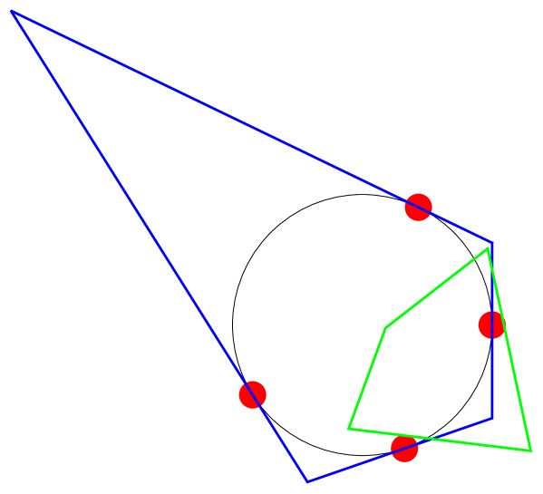
Figure 7: Inverse map. See [63].

The image under the inverse map with the incentre as pole seems often to take tangential quadrilateral vertices to points that look somewhat like vertices of a rhombus.

18 Bicentric polygons

In our calculations we often use $T_{k}$ as inout variables, or equivalently $\eta_{k}=\rho\,T_{k}$. There are additional identities for bicentrics beyond those that one has for tangential $n$-gons.

wikipedia gives, for bicentric quadrilaterals,

$\mathrm{bicentric4gon}:{\rho }^2={\eta }_1{\eta }_3={\eta }_2{\eta }_4.$

[71] studies bicentric hexagons and gives

$\mathrm{bicentric6gon}:{\rho }^2={\eta }_1{\eta }_3+{\eta }_3{\eta }_5+{\eta }_5{\eta }_1={\eta }_2{\eta }_4+{\eta }_4{\eta }_6+{\eta }_6{\eta }_2.$

There has been use of these in subsequent calculations.

The challenge put to me, admittedly in connection with $Q_{0-}$ rather than the geometric functionals treated in this Part IIb, is: investigate Blaschke-Santalo diagrams for tangential polygons. One triple that can be so investigated is $(\rho,L,R_{V})$ for bicentric polygons. For triangles, see the later section on Blundon’s inequality, e.g inequalities (19.1).

There is a huge literature on bicentric polygons dating back to the 19th century. The topics include Fuss’s Theorem, Poncelet’s porism and more. Some of this is impressive so is presented below - with nothing original of mine - but with the hope that some might be of use in future attempts to produce Blaschke-Santalo diagrams.

18.1 Fuss’s Theorem, Poncelet’s Porism

We would like to establish (polynomial) relations involving $(\rho,L,R_{V})$. Fuss’s theorem(s) involves $(\rho,R_{V},d)$ where $d$ is the distance between the circumcentre and incentre of the bicentric polygon. For triangles, The quantity $d$ can be recognized in Blundon’s inequality (19.1) and is, as in the first displayed equation below, $d=\sqrt{R_{V}(R_{V}-2\rho)}$.

The following is a (slightly adapted) quote from
https://mathworld.wolfram.com/PonceletsPorism.html

The three numbers $(\rho,R_{V},d)$ will not be arbitrary and along with $n$, they will have to satisfy certain relations. For the case of a triangle, one such relation is sometimes called the Euler triangle formula:

$$R_{V}^{2}-2R_{V}\rho-d^{2}=0.$$

One of popular notations for such relations (which is necessary and sufficient for existence of a bicentric polygon) can be given in terms of the quantities

$$a=\frac{1}{R_{V}+d},\ \ b=\frac{1}{R_{V}-d},\ \ c=\frac{1}{\rho}.$$

For a triangle, the Euler formula has the form:

$$a+b=c,$$

for a bicentric quadrilateral

$$a^{2}+b^{2}=c^{2}.$$

The relationship for a bicentric pentagon is

$$4(a^{3}+b^{3}+c^{3})=(a+b+c)^{3}.$$

Let

$$E_{1} = -a^{2}+b^{2}+c^{2},$$

$$E_{2} = a^{2}-b^{2}+c^{2},$$

$$E_{3} = a^{2}+b^{2}-c^{2}.$$

The relationship for a bicentric hexagon is

$$\frac{1}{E_{1}}+\frac{1}{E_{2}}=\frac{1}{E_{3}}$$

18.2 Triangles, again

The sides $s_{1}$, $s_{2}$, $s_{3}$ of a triangle are the roots of the cubic

$$y^{3}-Ly^{2}+(\frac{L^{2}}{4}+\rho^{2}+4\rho\,R_{V})y-2L\rho R_{V}=0.$$ (18.1)

ToDo. Find conditions on the coefficients of this cubic in order that it have 3 positive roots with the largest root less than the sum of the other two. Sturm sequences might be useful. Do Blundon’s inequalities come from this?

18.3 Bicentric quadrilaterals

The wikipedia article ‘Bicentric quadrilateral’ contains many items. There is a quartic equation with coefficients in terms of $L$, $\rho$ and $R_{V}$ whose solutions are the sides of a bicentric polygon:

$$y^{4}-Ly^{3}+(\frac{L^{2}}{4}+2\rho^{2}+2\rho{\sqrt{4R_{V}^{2}+\rho^{2}}})y^{2}-\rho L({\sqrt{4R_{V}^{2}+\rho^{2}}}+\rho)y+\rho^{2}\frac{L^{2}}{4}=0.$$ (18.2)

ToDo. Find conditions on the coefficients of this quartic in order that it have 3 positive roots with the largest root less than the sum of the other three. Sturm sequences might be useful.

There are huge number of inequalities.

Theorem.If a bicentric quadrilateral has an incircle and a vertex-circumcircle with radii $\rho$ and $R_{v}$ respectively, then its area $A$ satisfies

$$\frac{1}{2}\rho\,L=A\geq 2\rho\sqrt{2\rho(\sqrt{4R_{v}^{2}+\rho^{2}}-\rho)},$$

where equality holds if, and only if, the quadrilateral is also an isosceles trapezium.
See [36].
For a square $\rho=1$, $R=R_{v}=\sqrt{2}$, $A=4$ gives equality in the preceding inquality.

For a bicentric quadrilateral

$$\frac{1}{32}(L^{2}-16A)\leq R_{v}^{2}-\rho^{2}$$

with equality if and only if the hexagon is regular.

18.4 Bicentric hexagons

For a bicentric hexagon

$$\frac{1}{36}(L^{2}-8\sqrt{3}\,A)\leq R_{V}^{2}-\frac{4}{3}\rho^{2}$$

with equality if and only if the hexagon is regular.

For bicentric $n$-gons see [59].

18.5 $R=R_{v}=d_{O}$ for regular polygons

In a regular $n$-gon, the side $s_{n}=2\rho\tau_{n}$ where $\tau_{n}=\tan(\pi/n)$. The circumradius $R$ and $d_{O}$ coincide. We have

$$4(R^{2}-\rho^{2})=s_{n}^{2}$$

so

$$R=d_{O}=\sqrt{\rho^{2}+\frac{s_{n}^{2}}{4}}=\rho\sqrt{1+\tau_{n}^{2}}.$$

See Part IIa §8 for the formulae for $L=i_{0}$, $i_{2}$ and $i_{4}$.

18.6 Bicentrics from regular

Given any regular $n$-gon any choice of 3 of its vertices gives a bicentric polygon as all triangles are bicentric.

Given a regular 8-gon, selection of its alternate vertices gives a bicentric 4-gon, a square.

Given a regular 9-gon, there is a selection of 5 of its vertices giving a bicentric 5-gon. See [86, 87].

19 Blaschke-Santalo diagrams for tangential polygons

19.1 Definitions for Blaschke-Santalo diagrams

Where we feel it helps the exposition there will be some repetition of material already presented in PartIIa. We always choose the origin of our coordinate system to be at the incentre. The inradius $\rho$ and perimeter $L$ will occur in our diagrams, and there will be various choices of a third geometric quantity which, for the present, we denote by $q$. In our Blaschke-Santalo diagrams the horizontal axis is usually $x=L/q$ and the vertical axis $y=\rho/q$. (Further work in which $x=L/\rho$ and, as before, $y=\rho/q$ might be undertaken, motivated by having the same $x$ for the different $q$, e.g. $q$ being $i_{2}^{1/3}$, $Q_{0-}^{1/4}$, etc.) The area of a tangential polygon is $A=\rho\,L/2$. The quantity $x/y=L/\rho$ is denoted by $B$ in [69] . We have $B\geq{2\pi}$ with equality only for the disk, and for any triangle, $B\geq{6\sqrt{3}}$): see [1]. The perimeter and inradius of a regular $n$-gon are related by

$$\rho=\frac{L}{2n}\cot(\frac{\pi}{n}),$$

and for a tangential $n$-gon

$$B\geq{2n\tan(\pi/n)}.$$

The other domain functionals are as follows.
(1) There is a first set of geometric quantities:
$\bullet$ circumradius $R$ (radius of the smallest disk containing the region);
$\bullet$ the distance from the incentre to the boundary $d_{0}$;
(2) There are moments about the incentre:
$\bullet$ the second boundary moment $i_{2}$;
$\bullet$ the fourth boundary moment $i_{4}$;
(3) There are quantities leading to $Q_{0,-}$:
$\bullet$ $\Sigma_{\infty}=\rho\,i_{2}/16$;
$\bullet$ $0>\Sigma_{1}=(i_{2}^{2}/L-i_{4})/16$;
$\bullet$ $Q_{0-}$ the lower bound on torsional rigidity treated in Part I, i.e. [48].
We defer discussion of these last items, $Q_{0,-}$, until Part III.

In connection with bicentric polygons, including triangles, the radius of the circle through the vertices is denoted $R_{V}$, and we always have $R\leq{R_{V}}$.

An outline of the remainder of this section follows.

• In §19.2 we define cap domains which enter the account of the $(\rho,L,R)$ diagram in the next subsection.

• In §19.3 we present formulae for $d_{O}$ for various tangential $n$-gons.

• In §19.4 we begin by noting that the account for general convex domains in [10] has on one of its boundaries the 2-cap. We have done some computations, and have a belief that regular $n$-gons occur on one of the boundaries. However, the circumradius $R$ doesn’t seem to be a good lead-in for computations related to ($i_{2}$, $i_{4}$ and) $Q_{0-}$.

• §19.5 is the main subsection. The quantity $d_{O}$ is a function easily defined in terms of the $T_{k}$ occuring in expressions for $L$, $i_{2}$ and $i_{4}$, and hence in $Q_{0-}$. The expressions for $L$, $i_{2}$ and $i_{4}$ are given in Part IIa. The only Blaschke-Santalo diagrams presented here are those for $(\rho,L,d_{O})$. Future work may involve $(\rho,L,i_{2})$ and $(\rho,L,i_{2})$, but for now there is just occasional comment on relevant inequalities for particular tangential $n$-gons.

• Though we believe it to be an aside to our main purpose of investigating functionals related to $Q_{0-}$ over all tangential polygons, in §19.6 we propose to treat, for bicentric polygons the triple $(\rho,L,R_{V})$. So far, the main result is just that already in the literature for triangles. Some items in §18 may be useful in future efforts.

19.2 Some extremals amongst circumgons: the 1-cap and symmetric 2-cap

Because our long-term motivation concerns $Q_{0-}$ and this involves $i_{2}$ (and $i_{4}$) se begin with the following.

Let $\rho>0$. Among all plane convex sets $\Omega$ with fixed positive area $A$ (with $A>\pi\rho^{2}$) that contain a disk of radius $\rho$ around the origin, $i_{2}$ is maximized if $\Omega$ is the single-cap, the convex hull or a disk of radius $\rho$ and a point (the point being, up to rotation invariance, uniquely defined by the area constraint).
The proof is elementary. See [35] where it is a Lemma needed prior to establishing gradient bounds for the torsion function. Exactly the same proof gives the corresponding result for $i_{4}$.

Consider tangential polygons with $\rho$ and $d_{O}>\rho$ fixed. Amongst these the 1-cap
$\bullet$ minimizes $A$, $L$, $i_{2}$ and $i_{4}$ and
$\bullet$ minimizes $Q_{0}$.
This is because of domain monotonicity of these functionals.
Question. Given two tangential polygons $\Omega_{0}$ and $\Omega_{1}$ (with the same incentre? and) with $\Omega_{0}\subset\Omega_{1}$, is $Q_{0-}(\Omega_{0})\leq Q_{0-}(\Omega_{1})$?

            

Figure 8: Left: the symmetric 2–cap. Right: the 1-cap.

We can easily calculate the perimeter of the 1-cap. Denote by $\alpha$ the angle at its vertex on the circle radius $d_{O}$. Then $\sin(\alpha/2)=\rho/d_{O}$ and

$$L = (\pi+\alpha)\rho+2\sqrt{d_{O}^{2}-\rho^{2}},$$

$$\frac{L}{d_{O}} = \left(\pi+2\arcsin(\frac{\rho}{d_{O}})\right)\,\frac{\rho}{d_{O}}+\sqrt{1-(\frac{\rho}{d_{O}})^{2}}.$$

We will see this as occuring as the lower right boundary in diagrams with $x=L/d_{O}$, $y=\rho/d_{O}$. The limiting cases are

• $d_{O}\rightarrow\rho$, $y\rightarrow{1}$, $x\rightarrow{2\pi}$ corresponding to a disk;

• $d_{O}\rightarrow\infty$, $y\rightarrow{0}$, $x\rightarrow{2}$ corresponding to a long flat shapes like the 1-cap.

• $d_{O}\rightarrow\infty$, $y\rightarrow{0}$, $x\rightarrow{4}$ corresponding to a long flat shapes like the 2-cap.
  

• The quadrilateral might have one side tending to zero, say as a symmetric tangential trapezium tending to an isosceles triangle. When the squat isosceles triangle becomes very thin, $y\rightarrow{0}$, $x\rightarrow{4}$.

We will see the 2-cap in §19.4.

19.3 $d_{O}$ for various tangential $n$-gons

The distances from the incentre of the vertices of a tangential $n$-gon are given by

$$\sqrt{\rho^{2}+\eta_{k}^{2}}=\rho\sqrt{1+T_{k}^{2}}.$$

19.3.1 $R$, $d_{O}$ for regular polygons

In a regular $n$-gon, the side $s_{n}=2\rho\tau_{n}$ where $\tau_{n}=\tan(\pi/n)$. The circumradius $R$ and $d_{O}$ coincide. We have

$$4(R^{2}-\rho^{2})=s_{n}^{2}$$

so

$$R=d_{O}=\sqrt{\rho^{2}+\frac{s_{n}^{2}}{4}}=\rho\sqrt{1+\tau_{n}^{2}}.$$

See Part IIa §8 for the formulae for $L=i_{0}$, $i_{2}$ and $i_{4}$.

19.3.2 $R$, $d_{O}$ for triangles

For an equilateral triangle

$$L=6\sqrt{3}\rho,\qquad R=d_{O}=2\rho.$$

In general $R$ and $d_{O}$ differ. The circumradius of an acute angled triangle is the radius of the circle through the three vertices ($R=R_{V}$). For a triangle with one interior angle measuring more than $\pi/2$, an obtuse triangle, the circumradius is half the length of the longest side (and $R<R_{V}$).

For triangles equation (15.4) is

$$1-\frac{1}{T_{1}T_{2}}-\frac{1}{T_{2}T_{3}}-\frac{1}{T_{3}T_{1}}=0.$$

As in Part IIa, most of our calculations have, to date, concentrated on isosceles triangles. See Part IIa §9 for the formulae for $L=i_{0}$, $i_{2}$ and $i_{4}$. We return to triangles in §19.5.1. For now it is sufficient to record that

$\mathrm{triangle}:d_O=\rho \sqrt{1+\max {(T_1,T_2,T_3)}^2}.$

19.3.3 $d_{O}$ for tangential quadrilaterals

For tangential quadrilaterals equation (15.5) is

$$\frac{1}{T_{1}}+\frac{1}{T_{2}}+\frac{1}{T_{3}}+\frac{1}{T_{4}}-\frac{1}{T_{1}T_{2}T_{3}}-\frac{1}{T_{1}T_{2}T_{4}}-\frac{1}{T_{1}T_{3}T_{4}}-\frac{1}{T_{2}T_{3}T_{4}}=0.$$

We return to tangential quadrilaterals in §19.5.2. For now it is sufficient to record that

$\mathrm{tang}\mathrm{quad}:d_O=\rho \sqrt{1+\max {(T_1,T_2,T_3,T_4)}^2}.$

19.4 $(\rho,L,R)$

For any plane convex set

$$\rho\leq{R},\ L\leq{2\pi\,R},\ 2\pi\rho\leq{L},\ 4R\leq{L}.$$

There is some discussion of how to compute $R$ at
https://mathematica.stackexchange.com/questions/121987/how-to-find-the-incircle-and-circumcircle-for-an-irregular-polygon

We can scale our shapes so there is no loss of generality in setting $\rho=1$. Define

$$y=\frac{1}{R}\ \ {\rm and}\ \ x=\frac{L}{R},$$

(with our $x$ a factor of $2\pi$ greater than than in [10]).

$$x=2\pi,\ y=1\qquad{\rm for\ a\ disk}.$$

[10] establish, for convex sets,

$$4\left(\sqrt{1-y^{2}}+\ y\,{{\rm arcsin}(y)}\right)\leq x=\frac{L}{R}\leq 4\left(\sqrt{1-y^{2}}+{\rm arcsin}(y)\right).$$

The lower bound at the left corresponds to values for a symmetric 2-cap, which is a circumgon tangential polygon. However, the right-hand, upper bound is for a convex shape which is not a tangential polygon. Our computations suggest that amongst the tangential polygon shapes which will occur on the right-hand upper bound are the regular polygons.

In Figure 9 the right-most blue curve is the shape from [10] which is not a tangential polygon. The upper-left green curve is form the symmetric 2-cap. The red dots are some regular polygons, the rightmost upper dot the circular disk. The lowest is the equilateral triangle, and the next up, joining the upper blue curve is the square. The scatter of blue dots are from tangential quadrilaterals, and the upper blue line from rhombi.

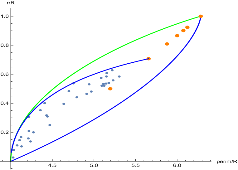
Figure 9: Except for the lower curve, some results on $(L/R,\rho/R)$ pairs for tangential polygons. See description in text.

19.5 $(\rho,L,d_{O})$

19.5.1 Triangles

See also PartIIa §9.

Amongst all isosceles triangles with given inradius

• the equilateral triangle minimizes $d_{O}$,

• the equilateral triangle minimizes $A$ and $L=2A/\rho$ and $L^{2}/A$, and

• the equilateral triangle minimizes $i_{2}$ and $i_{2}/(A\,L)$.

At given $\rho$ and $A$ greater than the area of the equilateral triangle of the same inradius, amongst isosceles triangles

• $d_{O}$ is maximised by tall isosceles triangles (apex angle $\alpha<\pi/3$ small, $\sigma<2-\sqrt{3}$ small)

• $d_{O}$ is minimised by short squat isosceles triangles (apex angle $\alpha>\pi/3$ near $\pi$, $\sigma>2-\sqrt{3}$ near 1).

(Above may be true for all triangles.)

The calculations for $i_{2}$ for the following are yet to be done.
Conjecture At given $\rho$ and $A$ greater than the area of the equilateral triangle of the same inradius, amongst isosceles triangles

• $i_{2}$ is maximised by tall isosceles triangles (apex angle $\alpha<\pi/3$ small, $\sigma<2-\sqrt{3}$ small)

• $d_{O}$ is minimised by short squat isosceles triangles (apex angle $\alpha>\pi/3$ near $\pi$, $\sigma>2-\sqrt{3}$ near 1).

19.5.2 Tangential quadrilaterals

Rhombi

Amongst all rhombi with given side,

• the square minimizes $d_{O}$,

• the square maximizes $A$ and $\rho=2A/L$, and

• the square minimizes $i_{2}/(A\,L)$.

These are easily established, as follows.

$$A=2\rho^{2}(T+\frac{1}{T})\qquad L=4\rho(T+\frac{1}{T}).$$

Hence

$$\frac{L^{2}}{A}=8(T+\frac{1}{T}),$$

which is minimized when $T=1$, the square.
Next

$$i_{2} = 2\rho^{3}\left(T+\frac{1}{T}+\frac{1}{3}(T^{3}+\frac{1}{T^{3}})\right),$$

$$= \frac{2\rho^{3}}{3}(T+\frac{1}{T})^{3},$$

so that

$$\frac{i_{2}}{AL}=\frac{1}{12}(T+\frac{1}{T}),$$

which is minimized at $T=1$.

We also have the following.

Amongst all rhombi with given inradius

• the square minimizes $d_{O}$,

• the square minimizes $A$ and $L=2A/\rho$ and $L^{2}/A$, and

• the square minimizes $i_{2}$ and $i_{2}/(A\,L)$.

A plot of $y=\rho/d_{O}$ against $x=L/d_{O}$ is shown in Figure 10

Figure 10: For rhombi, plot of $y=\rho/d_{O}$ against $x=L/d_{O}$. The top right corner is $(1/\sqrt{2},4\sqrt{2})$ corresponding to a square.

Kites

Amongst kites with given area $A$ and distance $d$ between apexes, the rhombus has

• the smallest perimeter $L$,

• the largest inradius $\rho=2A/L$, and

• the smallest $4I_{2}=\rho\,i_{2}$.

A proof uses Steiner symmetrisation.

One can easily recover results which, in a more general form, are given in the next subsubsection.

Amongst kites with given sides $s_{1}$ and $s_{2}$ the right kite has the largest area. For ease of writing, suppose $s_{1}<s_{2}$. The rhombus case can be treated separately. Let $h$ be the distance between the vertices adjacent to unequal sides. Let $\alpha_{1}$ be the angle at the vertex on both sides of length $s_{1}$. Denote by $\beta$, the repeated angle, the angle at vertices adjacent to the unequal sides.

$$A=\frac{1}{2}dh\ {\rm which\ can\ be\ written\ }\ A=s_{1}s_{2}\sin(\beta).$$

The formula at the right can be deduced from that on the left using the trigonometry:

$$h=2s_{1}\sin(\alpha_{1}/2),\qquad d=s_{2}\frac{\sin(\beta)}{\sin(\alpha_{1}/2)},$$

the latter from the triangle sine rule. Thus since $A=s_{1}s_{2}\sin(\beta)$, the area is maximized at $\beta=\pi/2$.

We remark

$$\rho = \frac{s_{1}s_{2}\sin(\beta)}{s_{1}+s_{2}},$$

$$\frac{L}{\rho} = \frac{2(s_{1}+s_{2})^{2}}{s_{1}s_{2}\sin(\beta)}.$$

Also, on using $s_{1}<s_{2}$,

$$\frac{d_{O}}{\rho}=\sqrt{1+{\rm max}(\cot(\frac{\beta}{2}),\cot(\frac{\alpha_{1}}{2}))^{2}},$$

and the sine rule for triangles gives $\alpha_{1}$ in terms of $s_{1}$, $s_{2}$ and $\beta$.

Other tangential quadrilaterals

For a quadrilateral with angles $\alpha_{k}$ and sequence of sides $[s_{1},s_{2},L/2-s_{1},L/2-s_{2}]$, the area is

$$A=\sqrt{s_{1}\,s_{2}\,(L/2-s_{1})\,(L/2-s_{2})}\sin(\frac{\alpha_{1}+\alpha_{3}}{2}).$$

For any quadrilateral, since the sum of the angles is $2\pi$,

$$\sin(\frac{\alpha_{1}+\alpha_{3}}{2})=\sin(\frac{\alpha_{2}+\alpha_{4}}{2})).$$

The formula for the area $A$ above gives the following.

Amongst all tangential quadrilaterals with given sequence of sides, the bicentric quadrilateral maximizes $A$ and $\rho=2A/L$.
A kite is bicentric iff it is a right kite.

In general, amongst all kites with a given pair of sides it is not the case that $i_{2}/(A\,L)$ is minimized by a right kite. (Let $\beta$ be the repeated angle in the kite. The quantity $i_{2}/(A\,L)$ plotted as a function of $1/\tan(\beta/2)$ appears to have a unique minimum which for a rhombus is at $\beta=\pi/2$, but in general is not.)

More on quadrilaterals

[53] treat quadrilaterals with diagonals intersecting at right angles. If the side lengths are denoted $s_{1}$, $s_{2}$, $s_{3}$, $s_{4}$ these satisfy

$$s_{1}^{2}+s_{3}^{2}=s_{2}^{2}+s_{4}^{2}.$$

If a quadrilateral is tangential and has its diagonals intersecting at right angles it is kite. (See also [52]

Bicentric quadrilaterals, $(\rho,L,d_{O})$

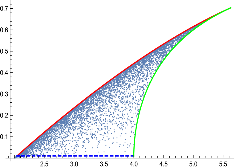
Figure 11: $x=L/d_{O}$, $y=\rho/d_{O}$ for bicentric quadrilaterals

The upper left boundary curve in Figure 11 (red) corresponds to right kites: the lower right curve (green) corresponds to tangential isosceles trapeziums. The dots are just from randomly generated tangential quadrilaterals. The uppermost point $(4\sqrt{2},1/\sqrt{2})$ corresponds to a square. The bottom boundary is approached by long thin shapes, and the left-most point is $(2,0)$ corresponding to the limit of thin shapes where $L\sim{2d_{O}}$.

Another approach to the boundary curves involves working with the tangent lengths $\eta_{j}$. For a bicentric quadrilateral with $\rho=1$ we have

$$\eta_{1}\eta_{3}=\rho^{2}=1=\eta_{2}\eta_{4}\ {\rm so}\ \ L=\eta_{1}+\frac{1}{\eta_{1}}+\eta_{2}+\frac{1}{\eta_{2}}.$$

Choose $\eta_{1}$ to be the largest of the $\eta_{k}$, so $\eta_{1}>1$ and $d_{O}=\sqrt{1+\eta_{1}^{2}}$. Now $\eta_{2}$ must be less than or equal to $\eta_{1}$ and greater than or equal to $1/\eta_{1}$, and consequently So

$$L_{-}=2+\eta_{1}+\frac{1}{\eta_{1}}\leq L\leq 2(\eta_{1}+\frac{1}{\eta_{1}})=L_{+}.$$

Plotting $y=1/d_{O}$ against $x=L_{-}/d_{O}$ gives one of the boundary curves, and the other is from $y=1/d_{O}$ against $x=L_{+}/d_{O}$.

As an aside we remark that for a bicentric quadrilateral for which $\rho=1$ and $s_{1}$ ia the largest side (so $s_{1}\geq{2}$) and $s_{2}$ is the larger of the other pair (so $s_{2}>1$),

$$L=\frac{s_{1}s_{2}(s_{1}+s_{2}+\sqrt{4+(s1-s2)^{2}}}{s_{1}s_{2}-1}.$$

General tangential quadrilaterals

In Figure 12 the scatter of (blue) points towards the left upper are from $T_{k}$ values with the first 3 not all that far from 1. (Those blue dots that are near the bottom come from those with $T_{4}$ large, such as occurs if the first 3 of the $T_{k}$ were near $1/\sqrt{3}$, the $\alpha_{k}$ near $2\pi/3$.) The red dots are from choosing the first 3 $T_{k}$ randomly in the interval $(0,1000)$. Large values of $T_{k}$ cause $d_{O}$ to be large, hence the cluster close to $y=0$. We haven’t definitively defined the boundaries. However we suspect the upper left boundary, at least for small enough $y$ ($d_{O}$ large) have the minimum $L$ shapes somewhat like the 1-cap, perhaps kites with a small apex angle at $d_{O}$.

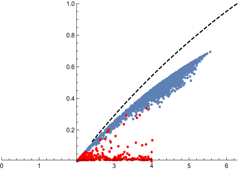
Figure 12: $x=L/d_{O}$, $y=\rho/d_{O}$ for tangential quadrilaterals

The dashed curve is the bound from the 1-cap, discussed nearthe beginning of this section.

19.5.3 Tangential pentagons

Bicentric pentagons

An elaborate formula for the area of a cyclic pentagon in terms of side lengths is given in [76].

19.5.4 Tangential hexagons

Bicentric hexagons

A question that arises is, what conditions other than

$$s_{1}+s_{3}+s_{5}=s_{2}+s_{4}+s_{6}=\frac{L}{2},$$

are satisfied by the sides, or tangent lengths $\eta_{j}$, for a bicentric hexagon. We have, for tangential hexagons,

$$s_{1}=\eta_{1}+\eta_{2},\ s_{2}=\eta_{2}+\eta_{3},\ s_{3}=\eta_{3}+\eta_{4},$$

$$s_{4}=\eta_{4}+\eta_{5},\ s_{5}=\eta_{5}+\eta_{6},\ s_{6}=\eta_{6}+\eta_{1},$$

or, in the notation of §15.1,

$$M(6)\,{\mathbf{\eta}}={\mathbf{s}}.$$

From [73] equations (2.29), (2.30)

$$\rho\sqrt{\frac{\eta_{1}\eta_{3}\eta_{5}}{\eta_{1}+\eta_{3}+\eta_{5}}}=\eta_{2}\eta_{5}=\eta_{1}\eta_{4}=\eta_{3}\eta_{6},$$

and, from [73] equation (2.26)

$$\eta_{1}\eta_{3}+\eta_{3}\eta_{5}+\eta_{5}\eta_{1}=\eta_{2}\eta_{4}+\eta_{4}\eta_{6}+\eta_{6}\eta_{2}=\rho^{2}.$$

Bicentric hexagons An elaborate formula for the area of a cyclic hexagon in terms of side lengths is given in [76].

19.6 $(\rho,R_{V},L)$ and generalizing Blundon’s inequality

We hope to treat bicentric quadrilaterals in the future, but, for now, here are results for triangles.

19.6.1 Triangles

One of the many entries in wikipedia’s list of triangle inequalities is the following, which in much of the literature is known as Blundon’s inequality:

$$2R_{V}^{2}+10R_{V}\rho-\rho^{2}-2\sqrt{R_{V}}(R_{V}-2\rho)^{3/2}\leq\frac{L^{2}}{4}\leq 2R_{V}^{2}+10R_{V}\rho-\rho^{2}+2\sqrt{R_{V}}(R_{V}-2\rho)^{3/2}.$$ (19.1)

Quoting from wikipedia:

Here the expression

$$\sqrt{R_{V}^{2}-2R_{V}\rho}={\rm dist(incentre,circumcentre)},$$

In the double inequality (19.1), the first part holds with equality if and only if the triangle is isosceles with an apex angle of at least $\pi/3$, and the last part holds with equality if and only if the triangle is isosceles with an apex angle of at most $\pi/3$. Thus both are equalities if and only if the triangle is equilateral.

Let $x=L/R_{V}$, $y=\rho/R_{V}$. The allowed values of the $(x,y)$ pair is the region inside the curves given by

$$4(2+10y-y^{2}-2(1-2y)^{3/2})\leq x^{2}\leq 4(2+10y-y^{2}+2(1-2y)^{3/2}),$$

and shown in Figure 13.

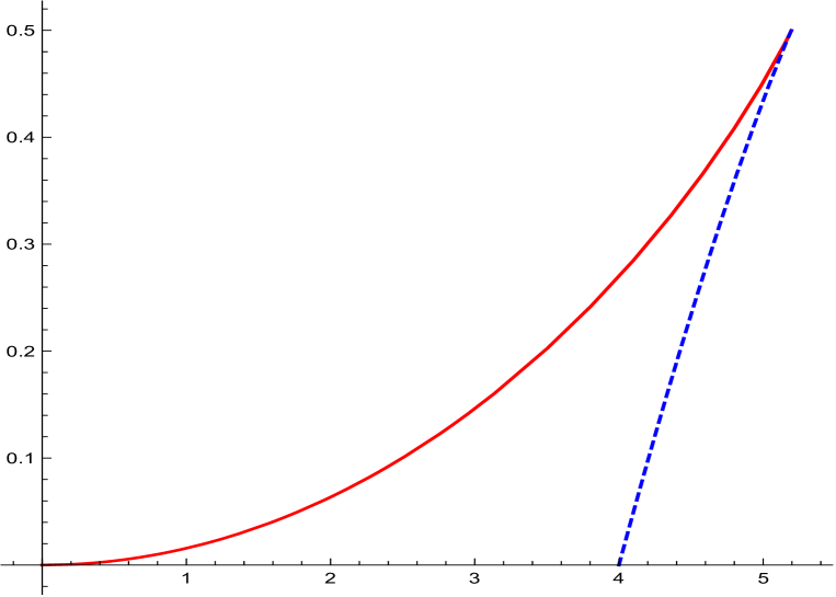
Figure 13: The lhs of the Blunden inequality is shown in red, the rhs in blue dashed.

Some of the behaviour of isosceles triangles for the various Blaschke-Santalo diagrams is indicated in the table below.

	squat	tall
$L/R$	$\sim{4}$	$\sim{4}$
$\rho/R$	$\rightarrow{0}$	$\rightarrow{0}$
$L/R$	$\sim{4}$	$\sim{2}$
$\rho/R$	$\rightarrow{0}$	$\rightarrow{0}$
$L/R_{V}$	$\sim{0}$	$\sim{4}$
$\rho/R_{V}$	$\rightarrow{0}$	$\rightarrow{0}$

20 Moments about the centroid, $I_{c}$

The moment of inertia about the centroid, $I_{c}$ is, amongst $n$-gons with a given area, minimized by the regular $n$-gon:

$$I_{c} \geq I_{c}({\rm reg-n-gon}),$$

$$= \frac{1}{4}\rho({\rm reg-n-gon})\,i_{2}({\rm reg-n-gon}),$$

$$= \frac{A^{2}(3+\tau_{n}^{2})}{6n\tau_{n}}\ {\rm where\ }\ \tau_{n}=\tan(\frac{\pi}{n}).$$

(The calculations for the equations above are in Part IIa.)

The St Venant inequality is the left-hand side below

$$\frac{Q_{0}}{A^{2}}\leq\frac{1}{8\pi}\leq\frac{I_{c}}{4A^{2}}\leq\frac{I_{2}}{4A^{2}},$$

where, as before, $I_{2}$ is the moment about the incentre, and, for tangential polygons, $I_{2}=\rho i_{2}/4$.

We can add this inequality into that near the end of Part I §3.2 that for any tangential polygon

$$\frac{1}{8}\rho^{2}A\leq Q_{0-}\leq Q_{0}\leq\frac{1}{4}I_{c}\leq\frac{1}{4}I_{2}\leq Q_{0+}.$$

20.1 Formulae for $I_{2}-I_{c}=A|z_{c}-z_{I}|^{2}$

The identity in the subsection heading is from the Parallel Axis Theorem.
https://en.wikipedia.org/wiki/Parallel_axis_theorem Denote by $z_{c}$ the coordinates of the centroid, and $z_{I}$ those of the incentre. Take, as elsewhere, the incentre to be the origin. Write

$$d_{IG}=|z_{c}-z_{I}|.$$

Triangles

For triangles $d_{IG}$ is given in terms of the side lengths in
https://mathworld.wolfram.com/Incenter.html
Let the sides be denoted by $s_{k}$ and define

$$S_{1} = s_{1}+s_{2}+s_{3},$$

$$S_{2} = s_{1}s_{2}+s_{2}s_{3}+s_{3}s_{1},$$

$$S_{3} = s_{1}s_{2}s_{3}.$$

Then

$$d_{IG}^{2}=\frac{5S_{1}S_{2}-S_{1}^{3}-18S_{3}}{9S_{1}}.$$ (20.1)

Quadrilaterals

For a rhombus the centroid and incentre coincide at the point of intersecion of the diagonals.

We have yet to derive, for tangential quadrilaterals or special cases of these, formulae analogous to (20.1).

See [53, 52] for results concerning centroids, and characterizations of kites, etc. See also [65, 31].

Part III: Other inequalities and properties for $Q_{0}$,
isoperimetric inequalities, etc.

Abstract for Part III

A referee asked for a bit more on ‘context’ and more numerics. There is a huge literature on bounds for torsional rigidity and in this part I focus on that most relevant to convex polygons.

• I also return to more on triangles, especially isosceles triangles for which, unsuprisingly, if one makes use of information specific to triangles, one can improve on my $Q_{0-}$ bound of Part I.

• Numerics for rhombi again indicate that $Q_{0-}$ is quite close to the actual torsional rigidity.

21 Introduction to Part III

A famous open problem is as follows.
Amongst all simple polygons with $n$ vertices with a given area, does the regular $n$-gon have the greatest torsional rigidity?
[69] establishes this for $n=3$ and $n=4$ but the question is open for $n>4$. It remains open for tangential $n$-gons too.
It will be easier to investigate, for tangential $n$-gons, this for the lower bound $Q_{0,c}$ rather than the actual torsional rigidity $Q_{0}$. The results in this direction are, so far, very slight (just isoceles triangles). We have yet to establish it for general triangles $n=3$.

An outline for this part is as follows.

• In §22 we present some previously published bounds. We also introduce the style of isoperimetric inequalities which will be studied in later sections.

• In §23 we review some bounds on $Q_{0}$.

• In §24 we study isosceles triangles There are many questions on how the geometry affects the domain functionals. We have, in §24.1, some isoperimetric results: some functionals are optimized, over isosceles triangles with given area, by the equilateral triangle.

• In §25 (yet to be written!) we will, very briefly, consider extending the work on $Q_{0-}$ to general triangles.

• In §26 we show, numerically for rhombi, how close $Q_{0-}$ is to $Q_{0}$.
  This parallels the work on isosceles triangles presented at the end of Part I.

• In §27 we consider Blaschke-Santalo diagrams involving $Q_{0}$, or $Q_{0-}$, for tangential polygons.

• In §28 I give further questions in connection with $Q_{0-}$. Some of these are of the form: if some property has been established for $Q_{0}$, does $Q_{0-}$ have the same property. Domain monotonicity is one such property, and one question is whether it remains, for $Q_{0-}$ under corner cutting (see Part IIb §12). Another, not discussed there, is whether, amongst tangential $n$-gons with a given inradius, the regular $n$-gon minimizes $Q_{0-}$.

22 Bounds on $Q_{0}$, esp. isoperimetric

Other papers involving the torsional rigidity of tangential polygons include [20]§2.2 involving web functions and [78]. Web functions are particularly simple for tangential polygons, and align with the similar level curves of [69], level curves which are the same shape as the boundary. In [78] the bounds are in terms of

$$I(q,\partial\Omega)=\int_{\Omega}{\rm dist}(z,\partial\Omega)^{q}.$$

(The notation is that of [42] as, in this Supplement, there are already other uses for $I$ and $i$. The capital $I$ is, as with our other use, an integral over the domain.) For tangential polygons $I_{0}(\partial\Omega)=|\Omega|$ and

$$I(q,\partial\Omega)=\frac{(p+1)(p+2)}{(q+1)(q+2)}I(p,\partial\Omega)\rho(\Omega)^{q-p}=\frac{1}{(q+1)(q+2)}\,|\Omega|\,\rho(\Omega)^{q}.$$

We specialise a much more general theorem of [78] to the following.
Theorem [78]. Let $\Omega$ be a tangential polygon. Then

$$Q_{0}(\Omega)\geq\frac{1}{16}(p+1)(p+2)I(p,\partial\Omega)\,\rho(\Omega)^{2-p}\qquad{\rm where}\ -1\leq p<\infty.$$

Equality holds if $\Omega$ is a disk.
In particular, with $p=2$

$$\frac{1}{2}|\Omega|\rho^{2}=3I(2,\partial\Omega)\leq 4Q_{0}(\Omega),$$

which recovers [69]§5.8 equation(7) on p100. See inequality (1.4) in Part I. [78] is largely concerned with how this might generalize to domains other than tangential polygons.

The famous open problem stated at the beginning of this part is as follows.
Amongst all simple polygons with $n$ vertices with a given area, does the regular $n$-gon have the greatest torsional rigidity?
Repeating from there: [69] establishes this for $n=3$ and $n=4$ but the question is open for $n>4$.

Of course the question can be asked with a smaller sets, e.g. convex polygons or tangential polygons or bicentric polygons or … To date there are no answers for the torsional rigidity. There are, however, for some other domain functionals: see Part IIb for purely geometric ones. The conformal inradius and related radii are others that on fixing the area is extreme for the regular $n$-gon (see [83]). By a $\cal D$ we shall mean some domain functionals, and we are interested in pairs of these for which one has a result of the form
For tangential $n$-gons with fixed ${\cal D}_{1}$ the regular $n$-gon $<$maximizes$|$minimizes$>$ ${\cal D}_{2}$
Table 6 below presents some (repeating some entries from Table 4 of Part IIb):

${\cal D}_{1}$		${\cal D}_{2}$	Remark
area	min	perimeter
area	max	inradius	$A=\rho L/2$
inradius	min	perimeter	Jensen inquality
inradius	min	area	”
inradius	min	$Q_{0}$	Solynin [82, 84]
			see below

Table 6: Tangential polygons

In [82] the result, at fixed inradius $\rho$, that $Q_{0}$ is minimized at the regular $n$-gon is first given, in Theorem 1, for tangential $n$-gons, and, after that, in Theorem 2, for more general $n$-gons. (I have yet to check the proofs.)

22.1 Bounds on $Q_{0}$ for convex $\Omega$

We have, in Part I, reported the results, from [69]

$$\frac{A^{2}}{4B}\leq Q_{0}\leq\frac{A^{2}}{8\pi}.$$

The left-hand inequality is in Part I, inequality (1.4): the right-hand inequality is the St Venant Inequality. There is equality in both for disks. [69] p99 gives, for convex domains,

$$B\leq\frac{2A}{\rho^{2}},$$

which is an equality for tangential polygons. Combining these gives for convex domains, the left-hand inequality in

$$\frac{1}{8}\rho^{2}A\leq Q_{0}\leq c\rho^{2}A.$$

The left hand inequality is from [69]§5.8 equation (7), and equality occurs for $\Omega$ a disk. The right hand inequality with $c=\frac{1}{3}$ is one of several due to Makai, and equality is approached by rectangles as they become long and slender, leaving the question as to the best constant $c$ when restricted to tangential polygons.

From [69] p254, for a thin rectangle

$$Q_{0}\sim\frac{1}{3}\rho^{2}A\ \ {\rm for}\ \ \rho\rightarrow{0}.$$

For thin isosceles triangles, with small vertex angle,

$$Q_{0}\sim\frac{1}{6}\rho^{2}A\ \ {\rm for}\ \ \rho\rightarrow{0}.$$

For the lower bound found in Part I

$$Q_{0,-}\sim\frac{21}{128}\rho^{2}A\ \ {\rm for}\ \ \rho\rightarrow{0}.$$

This checks with $Q_{0-}\leq Q_{0}$.

Another inequality for convex domains is

$$\frac{1}{3}\frac{A^{3}}{L^{2}}\leq Q_{0}\leq\frac{2}{3}\frac{A^{3}}{L^{2}}.$$

The left inequality is approached by thin rectangles. The right inequality is approached by thin acute isosceles triangles. (It is curious that thin rectangles occur as upper bounds in one inequality in this section, and lower bounds in another.) However, inequalities for convex sets,

$$\frac{\rho}{2}\leq\frac{A}{L}\leq\rho(1-\frac{\pi\rho}{L})\leq\rho,$$

(in which the central inquality is equality for a disk, [80]) are consistent with

$$\frac{1}{3}\frac{A^{3}}{L^{2}}\leq Q_{0}\leq\frac{1}{3}\rho^{2}A.$$

For tangential polygons the inequalities above give

$$\frac{1}{2}\frac{A^{3}}{L^{2}}=\frac{1}{8}\rho^{2}A\leq Q_{0}\leq\frac{1}{6}\rho^{2}A=\frac{2}{3}\,\frac{A^{3}}{L^{2}}.$$

The extreme domains are the disk (left) and thin isosceles triangles (right).

See also [14].

22.2 Cheeger constant and $Q_{0}$

We have

$$Q_{0}(\Omega)h(\Omega)^{4}\geq Q_{0}(B)h(\Omega)^{4}=2\pi.$$

Equality occurs only for disks. See [57], and specialize to 2-dimensions. Thus for our tangential polygons

$$Q_{0}(\Omega)\geq\frac{32\pi A^{4}}{(L+\sqrt{4\pi A})^{4}}.$$

Much is known about the elastic torsion function and, in particular, its properties in convex domains.

It is known that in convex $\Omega$, the square root of the torsion function $\sqrt{u_{0}}$ is concave. In some proofs of this one uses that for solutions of the torsion equation $\log(1-4H)$, with H the hessian determinant, is harmonic. $u_{0}$ is, itself, not concave in any domain with corners. However one can ask on what subset $\Omega_{1}$ of $\Omega$ is $u_{0}$ concave. For an equilateral triangle (and for a disk), $\Omega_{1}$ contains the incircle. (See §11 of [45].) One wonders what additional conditions, if any, might be needed for it to happen in other tangential polygons that $\Omega_{1}$ contains the incircle.

Improvements on the St Venant inequality involving Fraenkel asymmetry are given in [11].

There is a Urysohn’s type inequality which we denote by (U).
(U): among convex sets with given mean width, the torsional rigidity is maximized by balls.
The mean width $w$ of any compact shape $\Omega$ in two dimensions is $L/\pi$, where $L$ is, as before, the perimeter of the convex hull of $\Omega$. So $w$ is the diameter of a circle with the same perimeter as the convex hull. So in (U) it is just maximizing with same perimeter. Inequality (U) is weaker than St Venant.

There are inequalities involving polar moment of inertia about the centroid.
For convex domains $Q_{0}I_{c}A^{-4}$ is maximized by its value for an equilateral triangle. (Related results, if not exactly this, are in [68].)
We conjecture:
For tangential polygons $Q_{0}I_{2}A^{-4}$ is maximized by its value for an equilateral triangle.

Sperb $u_{\rm max}\leq\rho^{2}$. Strip $u_{0}=(\rho^{2}-x^{2})/2$

23 Some bounds on $Q_{0}$

Recall the well-known estimates

$$Q_{0} \leq \frac{\pi}{8}\,\left(\frac{A}{\pi}\right)^{2}=Q_{\odot,0},$$

$$Q_{0} \leq \Sigma_{\infty}.$$

Define, in the notation of [69],

$$B_{\Omega}=\int_{\partial\Omega}\frac{1}{x\cdot{n}}.$$ (23.1)

Some well known lower bounds are:

$$Q_{0} \geq \frac{A^{2}}{4\ B_{\Omega}}(={\rm{\ for\ tangential\ polygons\ }}\frac{A^{3}}{2L^{2}}),$$

$$Q_{0} \geq \frac{\pi}{8}\,{\dot{r}}^{2},$$

where ${\dot{r}}$ is the maximum interior mapping radius of $\Omega$.

24 More on isosceles triangles

24.1 Isoperimetric inequalities for isosceles triangles

Numerical data on functionals associated with isosceles triangles was given in§9. Our main emphasis in the following will be isosceles triangles rather than general triangles. However, some general statements are available. Recall that $\cal A$ is all (simply-connected) domains, ${\cal A}_{n}$ is all $n$-gons.

• $Q_{0}/A^{2}$ is maximized over ${\cal A}_{3}$ (triangles) for an equilateral triangle.

• $B=L/\rho$ is minimized over ${\cal A}_{3}$ (triangles) for an equilateral triangle.

• ${\dot{r}}/\sqrt{A}$ is maximized over ${\cal A}_{3}$ (triangles) for an equilateral triangle.

24.1.1 $B$

$B=L/\rho$ for any tangential polygon, so for isosceles triangles in particular.
The disk minimizes $B$ and $Q_{0}B/A^{2}$ over tangential polygons.
The equilateral triangle minimizes $B$ and $Q_{0}B/A^{2}$ over triangles.

shape	$n$	$8\pi Q_{0}/A^{2}$	$Q_{0}/(A/\pi)^{2}$	$B=\frac{L}{\rho}$	$4Q_{0}B/A^{2}$
disk	$\infty$	1	$\pi/8$	$2\pi$	$1$
hexagon	6	0.9643	0.3786	$4\sqrt{3}$	$1.063$
square	4	0.8834	0.3469	$8$	$1.125$
equilateral $\Delta$	3	0.7255	0.2849	$6\sqrt{3}$	$1.200$
right isosceles		0.6557	0.2575	$4(1+\sqrt{2})$	$1.217$

24.1.2 $\dot{r}$

The calculation of $\dot{r}$ for polygons often involves the use of Schwarz-Christoffel conformal mappings. Some exact values are given on p273 of [69].

• (Aside, except for $n=3$.) For a regular polygon with $n$ sides, and perimeter $L_{n}$,

  $${\dot{r}}_{n}=\frac{\Gamma(1-\frac{1}{n})}{2^{1+2/n}\,\Gamma(\frac{1}{2})\,\Gamma(\frac{1}{2}+\frac{1}{n})}\,L_{n}.$$

• Again citing [69] p158, amongst all triangles with a given area that which maximizes $\dot{r}$ is equilateral.

• For (regular polygons and) triangles we have

  $$\pi{\dot{r}}{\bar{r}}=A,$$

  $A$ being the area and $\bar{r}$ the transfinite diameter.

• Working from earlier more general results (Haegi 1951) in [22] it is given that for an isosceles triangle, vertex angle $\alpha$ and base $2\sin(\alpha/2)$ the transfinite diameter, denoted there by $\kappa$, is

  $$\kappa(\alpha)=\frac{\sqrt{\pi+\alpha}}{8\pi^{5/2}}\left(\frac{\pi+\alpha}{4\alpha}\right)^{\alpha/(2\pi)}\,\frac{\sin(\alpha)^{2}}{\sin(\alpha/2)}\,\Gamma(\frac{\alpha}{\pi})\,\Gamma(\frac{\pi-\alpha}{2\pi})^{2}.$$

For isosceles triangles with area $A$ and vertex angle $\alpha$

$${\bar{r}}=\frac{2\sqrt{A\tan(\alpha/2)}}{\sin(\alpha/2)}\,\kappa\ \ {\rm so\ \ }{\dot{r}}=\frac{A}{\pi{\bar{r}}}=\sqrt{A}\,\frac{\sin(\alpha/2)}{2\pi\sqrt{\tan(\alpha/2)}}\,\frac{1}{\kappa}.$$

Some values of $\dot{r}$, as given in [69], are copied in the following table.

shape		$\dot{r}$	$\dot{r}$	$\frac{\dot{r}}{\sqrt{A}}$	$8Q_{0}/(\pi{\dot{r}}^{4})$
disk	radius $a$	$a$	$a$	$0.56419$	$1$
hexagon	side $s_{6}$	$\frac{2^{5/3}\,\sqrt{3}\pi}{\Gamma(1/3)^{3}}\,s_{6}$	$0.89850s_{6}$	$0.55744$	$1.011$
square	side $s_{4}$	$\frac{4\sqrt{\pi}}{\Gamma(1/4)^{2}}\,s_{4}$	$0.53835s_{4}$	$0.53935$	$1.058$
equilateral $\Delta$	side $s_{3}$	$\frac{2\pi}{\Gamma(1/3)^{3}}\,s_{3}$	$0.3268\,s_{3}$	$0.49665$	$1.209$
right isosceles	equal sides $a$	$\frac{4\sqrt{2\pi}}{3^{3/4}\,\Gamma(1/4)^{2}}\,a$	$0.33462a$	$0.47320$	$1.325$

24.1.3 Simple comments on torsion for isosceles triangles

As noted before, for an equilateral triangle the torsion function is a cubic polynomial in $x$ and $y$ corresponding to forming the products of three linear terms, each linear term being 0 on one side of the triangle. There appear to be no other simple solutions for isosceles triangles, though there is a series formula for the torsional rigidity of the right isosceles triangle.

In the table below, in the second, third and fourth columns we take the base to be 2, the area to be $h$, $h$ being the height; in the fifth and sixth columns the area is $\sqrt{3}$, the height is $h$ and the base $2\sqrt{3}/h$.

infinitely acute	$h\rightarrow\infty$	$A\sim{h}$	$Q_{0}\sim\frac{1}{6}h$	$h\rightarrow\infty$	$Q_{0}\sim\frac{1}{2h}$
equilateral	$h=\sqrt{3}$	$A=\sqrt{3}$	$Q_{0}=\frac{\sqrt{3}}{20}$	$h=\sqrt{3}$	$Q_{0}=\frac{\sqrt{3}}{20}$
right isosceles	$h=1$	$A=1$	$Q_{0}=0.026091$	$h=3^{1/4}$
infinitely flat	$h\rightarrow{0}$	$A\sim{h}$	, $Q_{0}\sim\frac{1}{24}h^{3}$	$h\rightarrow{0}$	$Q_{0}\sim\frac{h}{8}$

24.1.4 More variational bounds on $Q_{0}$ for isosceles triangles

The bounds on $Q_{0}$ we report here are often very old.

There are, of course, variational formulations of the Problem (P(0)). For positive, differentiable functions $v$, let

$$E(v,0,k)=\int_{\Omega}v^{k}\qquad{\rm and\ \ }E(v,1,k)=\int_{\Omega}|\nabla v|^{k}\ .$$

With

$$Q_{0,\rm LB}(v)=E(v,0,1)^{2}/E(v,1,2)$$ (24.1)

it can be shown that for any smooth function $v$ vanishing on the boundary of $\Omega$, the expression $Q_{0,\rm LB}(v)$ provides a lower bound on the torsional rigidity $Q_{0}=Q_{0,\rm LB}(u)$. The theory for this is given in [69].

For isosceles triangles, base $2a$, height $h$, a simple trial function $v$ to substitute into (24.1) is

$$v_{\rm cub}=(y+\rho)(1-(x/a)-((y+\rho)/h))(1+(x/a)-((y+\rho)/h)).$$ (24.2)

Evaluating the integrals gives

$$Q_{0\rm{cub}}=Q_{0,\rm LB}(v_{\rm cub})=\frac{a^{3}h^{3}}{(30a^{2}+10h^{2})}=\frac{A^{2}}{30\tau+10/\tau},$$ (24.3)

with $\tau=a/h=\tan(\alpha/2)$ as before, and the expression on the right of (24.3) is, in fact, an approximation given in Roark’s tables, valid for the the vertex angle $\alpha$ of the isosceles triangle lying between 40 and 80 degrees. It is exact for the equilateral case where the vertex angle is 60 degrees. It would, we think, be an improvement to Roark’s tables to have noted, after defining this rational function of $a$ and $h$, to have noted that $Q_{0}>Q_{0,\rm LB}(v_{\rm cub})$ for all positive values of $a$ and $h$, and after this to have noted the range of $h/a$ over which it provides a good approximation to $Q_{0}$.

We can compare this lower bound with our earlier $Q_{0-}$ as shown in Figure 1. In the next figures the bound of (24.3) is shown brown, dashed. Unsurprisingly it is good for triangles near equilateral improving on $Q_{0-}$ there, but it is worse than $Q_{0-}$ when not near equilateral. For example, for a right isosceles triangle, with area $\sqrt{3}$ we found

$$Q_{0}=0.07827,\qquad Q_{0-}=0.07651,\qquad Q_{0\rm{cub}}=\frac{3}{40}=0.075.$$

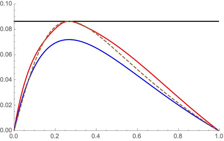
Figure 14: For an isosceles triangle with area$\sqrt{3}$. $\sigma$ is tan of 1/4 of the apex angle. Blue is $Q_{B}$, red is the new lower bound $Q_{0-}$, black is $Q_{\Delta}$, brown dashed is the cubic one underdiscussion.

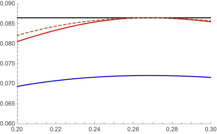
Figure 15: For an isosceles triangle with area$\sqrt{3}$. $\sigma$ is tan of 1/4 of the apex angle. Blue is $Q_{B}$, red is the new lower bound $Q_{0-}$, black is $Q_{\Delta}$, brown dashed is the cubic one underdiscussion.

Define $v_{\rm quad}$ to be even in $x$ and

$$v_{\rm quad}=y(1+(x/a)-(y/h))\ \ {\rm for}\ \ 0<x<a.$$

Good lower bounds on $Q_{0}$ for when $h$ is small can be found using this as test function.

See PartI, near Figure 2 for another lower bound on $Q_{0}$. Many other bounds are available. See for example the Appendix, by Helfenstein of the paper [67].

ToDo. Check the Helfenstein work. Stretching in one direction Define

$$D(1,t)=\{(tx,y)|(x,y)\in D\}.$$

In particular, $D(1,1)=D$. Domain monotonicity gives $QQ_{0}(D(1,t))$ is increasing in $t$. In [67] it is shown that $t/Q_{0}(D(1,t))$ is increasing and concave in $t^{2}$. The appendix to their paper by Helfenstein makes good use of this in connection with isosceles triangles, finding upper and lower bounds on $Q_{0}$ which differ by no more than 12%. These are, unfortunately, rather elaborate, and with cheap numerical computing, it is perhaps better to use the stretching result as yet another check on numerics.

ToDo. Main interest is in $Q_{0}(D(1,t))/|D(1,t)|^{2}$ where the maximum occurs for $t$ giving an equilateral triangle.

24.2 Miscellaneous other bounds

Consider an isosceles triangle with a base of length 2 and height of length $h$, and angles $\beta$, $\beta$, and $\pi-2\beta$ respectively. Since $\tan(\beta)=h$, and the area $A$ of the triangle is $h$, it can be shown that an inequality from [9] is

$$Q_{0}\leq\frac{1}{8}(1+A^{2})^{2}\,(A-{\rm arctan}(A)).$$

This inequality is, in [9], used with triangles which are thin, and, while satisfied for equilateral, it is weak there.

25 General triangles

From the calculations of $L$, $i_{2}$ nad $i_{4}$ in Part IIb §16, $\Sigma_{\infty}$ and $\Sigma_{1}$ can be found.

26 Rhombi

The formulae for $A$, $L$, $i_{2}$, $i_{4}$, $\Sigma_{\infty}$, $\Sigma_{1}$ are given in Part IIa §10. The numerical values of $Q_{0}$ are from [79] (and checked with Mathematica NDSolve).

Figure 16: Rhombus

27 Blaschke-Santalo for $Q_{0}$

If one were to assemble, for tangential polygons with given $\rho$ and $d_{O}$, a Blaschke-Santalo diagram, I would expect that with $Q_{0}$ would be similar to that with the area (or equivalently the perimeter) given earlier. In particular, at given $\rho$ and $d_{O}$,

• the 1-cap would minimize $Q_{0}$ thereby providing the left-upper boundary in the diagram, and

• the regular polygons would be amongst the maximizing shapes thereby providing a scatter of points on the right-lower boundary.

There may be independent interest in curves, or other subsets, in the region, e.g. for

• triangles

• kites/rhombi
  other quadrilaterals.

A much easier task is to find the diagram for the lower bound $Q_{0-}$. I expect everything stated above for $Q_{0}$ would occur in this simpler situation.

28 Further questions

Question. Does ‘corner cutting’ (defined in §12) increase $Q_{0}/A^{2}$?
It would be (much) easier to begin with $Q_{0-}$ and isosceles triangles each having its apex corner cut to form a symmetric tangential trapezium.

Given the area of a regular $n$-gon, its inradius is, as in Part IIa §8,

$$\rho_{n}^{2}=\frac{A}{n\tau_{n}}\qquad{\rm with\ \ }\tau_{n}=\tan(\frac{\pi}{n}).$$

Formulae for $i_{2,n}$, $i_{4,n}$, $\Sigma_{1,n}$ and $\Sigma_{\infty,n}$ are also given in Part IIa §8. Let $f_{n}(Q_{0})$ be the quadratic in $Q_{0}$ defined at Part I, equation (3.6) using the values appropriate to the regular $n$-gon for $\rho$, $i_{2}$ and $i_{4}$. The leading coefficient, i.e. coefficient of $Q_{0}^{2}$, is the same for the two polynomials.

For an equilateral triangle with area $\sqrt{3}$, we found in Part I

$$f_{3}(Q_{0})=f_{\Delta}(Q_{0})=32\sqrt{3}(Q_{0-}\frac{\sqrt{3}}{20})(Q_{0}-\frac{\sqrt{3}}{4}).$$

We wish to show that, for any tangential $n$-gon with the same area

$$Q_{0-}\leq Q_{0-,n}.$$

This suggests that we try to show

$$f(Q_{0,n})\leq{0},\qquad f_{n}(Q_{0})\geq{0}.$$

This leads to the question of how roots of a quadratic change when its coefficients change. Both polynomials $f$ are of the form

$$32A(Q_{0}^{2}+b*Q_{0}+c)=0,$$

with two positive roots

$$2\sqrt{c}<b<0,\qquad 0<c<\frac{b^{2}}{4}.$$

If we could show that both coefficients $b$ and $c$ are largest for the regular $n$-gon case, this would establish that $Q_{0,n}$ was larger than any other tangential $n$-gon.

It would seem prudent

• to begin with $n=3$,

• then $n=4$, initially with special cases (rhombi, kites, etc.)

• then $n=5$,

• then $n=6$,

• then general $n$.

Part IV: Robin boundary conditions $Q(\beta)$,
isoperimetric inequalities, etc.

29 Robin boundary conditions

Part IV concerns a different problem than the earlier parts.

The function $R$ of [47] is a function of a nonnegative parameter $\beta$ and geometric functionals $A$, $L$, $\Sigma_{\infty}$ and $\Sigma_{1}$ and $Q_{0}$. Knowledge of these, for triangles, (as in Part II) is essential for the following questions.

Let $\beta\geq{0}$. For solutions $u_{\beta}$ of Problem (P($\beta))$ of [47] in a triangle define $Q_{\rm triangle}(\beta)$ as the integral of $u_{\beta}$ over the triangle.

Question. Consider triangles of fixed area, say $\sqrt{3}$. Amongst these triangles is that which has the greatest $Q(\beta)$ the equilateral triangle?
(For $\beta=0$ this is the case as proved in [69].) (A similar question, but for the fundamental frequency is asked in [55].)

In [47] we presented a lower bound $R(\beta,\ldots)$ for $Q(\beta)$ and noted that it provided a good approximation to $Q(\beta)$. For triangles the only argument of $R$ that isn’t a relatively simple function of the triangle’s geometry is the torsional rigidity $Q_{0}$. This leads on to simpler questions (for which some of Part III might be relevant).

Question. Consider triangles of fixed area, say $\sqrt{3}$. What additional properties of the torsional rigidity $Q_{\rm triangle}(0)$ will ensure that for these triangles that which has the greatest $R(\beta,\ldots)$ is the equilateral triangle?

Questions. Consider triangles of fixed area, say $\sqrt{3}$. Replacing, in $R(\beta,\ldots)$, $Q_{\rm triangle}(0)$ by one of its bounds or approximations, will ensure that for these triangles that which has the greatest $R(\beta,\ldots,Q_{0,{\rm approx}})$ is the equilateral triangle?
(The plural in ‘Questions’ is because there are several possible bounds that might be used.)

There is some indication via numerics that, restricting to isosceles triangles, equilateral triangles maximize.

More generally, similar questions can be asked for $n$-gons. For these, does the regular $n$-gon optimize?

Part V: Miscellaneous PDE and tangential polygons

Tangential polygons get a mention in other pde papers.

Papers by Solynin include treatment of the fundamental frequency for tangential $n$-gons.

Consider evolution of temperature satisfying the heat equation, zero Dirichlet data on boundary of a convex plane domain $C$, and unit initial value. In the convex domain $C$ there will, at each fixed time, be a unique point at which the solution is a maximum, hot-spot. [58] characterises the tangential polygons which have stationary hot-spots, basically as the regular polygons. We remark that the integral of the solution to the heat equation, integrated w.r.t. time $t$ from 0 to infinity, solves the torsion problem. So the unique maximum of the torsion function would have to be the stationary hot-spot. They must coincide with the unique critical point of the first eigenfunction. What further restrictions are needed on a tangential polygon in order that the incentre is a stationary hot spot?

References

-
[1]
M.I. Aissen (1958)
A set function defined for convex plane domaines, Pacific Journal of Mathematics 8(3), 383–399.
doi:10.1115/1.4004591 -
[2]
T.M. Apostol and M.A. Mnatsakanian (2004)
Figures circumscribing circles,
American Mathematical Monthly 111, 853–863.
doi:10.2307/4145094
T.M. Apostol (December 2005). erratum, American Mathematical Monthly 112 (10): 946. -
[3]
C. Audet, P. Hansen and F. Messine (2009)
Extremal problems for convex polygons – an update,
In book:
Lectures on global optimizationEdition Amer. Math. Soc., Providence, RIPublisher:.
DOI: 10.1090/fic/055/01 - [4] A. Baernstein (2006) Dubinin’s symmetrization theorem. pp23–30 in Complex Analysis I, Lecture Notes in Mathematics book series (LNM, volume 1275)
- [5] R. Banuelos, M. Van den Berg, T. Carroll (2002) Torsional rigidity and expected lifetime of Brownian motion, Journal of the London Mathematical Society 66(2), 499–512
-
[6]
M. van den Berg and G. Buttazzo (2020)
On capacity and torsional rigidity,
Bull.Lond.Math.Soc.
http://cvgmt.sns.itand athttp://www.arxiv.org
arXiv preprint 2001.04421 5 -
[7]
M. van den Berg, G. Buttazzo and A. Pratelli (2019)
On the relations between principal eigenvalue and torsional rigidity,
Commun. Contemp. Math.
http://cvgmt.sns.itand athttp://www.arxiv.org
arXiv 1910.1459 - [8] M. van den Berg, V. Ferone, C. Nitsch, and C. Trombetti (2016) On Polya’s inequality for torsional rigidity and first Dirichlet eigenvalue, Integral Equations Operator Theory 86(4), 579–600.
-
[9]
M. van den Berg, V. Ferone, C. Nitsch, and C. Trombetti (2020)
On a Polya functional for rhombi, isosceles triangles, and thinning convex sets,
Revista Matematica Iberoamericana 36(7), 2091–2105.https://doi.org/10.4171/rmi/1192 - [10] K. Boroczky, M.A. Cifre, G. Salinas (2003) Optimizing area and perimeter of convex sets for fixed circumradius and inradius, Monatshefte fur Mathematik, 138, 95–110.
- [11] L. Brasco and G. de Philippis (2016) Spectral inequalities in quantitative form.
-
[12]
C.J. Bradley (2006)
Hexagons with Opposite Sides Parallel,
Mathematical Gazette 90(517), 57–67.
doi: 10.1017/S0025557200179033 -
[13]
R. Brandenberg and B.G. Merino (2016)
A complete 3-dimensional Blaschke-Santalo diagram,
Mathematical Inequalities and Applications 20(2).
doi: 10.7153/mia-20-22 -
[14]
Luca Briani, Giuseppe Buttazzo and Francesca Prinari (2020)
Some inequalities involving perimeter and torsional rigidity,
Applied Mathematics and Optimization
https://doi.org/10.1007/s00245-020-09727-7
arXiv:2007.02549 - [15] M.W. Buck and R.L. Siddon (2005) The area of a polygon with an inscribed circle, arXiv:1203.3438
- [16] D. Bucur and I. Fragala (2016) A Faber-Krahn inequality for the Cheeger constant of -gons, The Journal of Geometric Analysis 26, 88–117.
-
[17]
D. Bucur and I. Fragala (2020) Symmetry results for variational energies on convex polygons,
ESAIM: Control, Optimisation and Calculus of Variations
DOI: https://doi.org/10.1051/cocv/2020083z
Preprint 2020http://cvgmt.sns.it/media/doc/paper/4796/polygons.pdf - [18] W. Chao and P. Simeono (2000) When quadrilaterals have inscribed circles (solution to problem 10698), American Mathematical Monthly 107(7), 657–658.
- [19] M.J.Crabb, J.Duncan, C.M.McGregor (20??) Par-hexagons.
- [20] Crasta, G., Fragala, I. & Gazzola, F. (2002), A sharp upper bound for the torsional rigidity of rods by means of web functions, Archive for Rational Mechanics and Analysis, bf 164(3), 189–211. doi: 10.1007/s002050200205
- [21] S.S. Dragomir and G. Keady (2000) A Hadamard-Jensen inequality and an application to the elastic torsion problem, Applicable Analysis
-
[22]
S. Finch (2014)
Appell and conformal mapping,
http://arxiv.org/abs/1408.1074 - [23] S. Finch (2014) Fraenkel asymmetry.
- [24] Fragala, I., Gazzola, F., Lamboley, J. (2013) Some sharp bounds for the p-torsion of convex domains, Geometric Properties for Parabolic and Elliptic PDE’s, vol. 2, 97–115. Springer INdAM Series, Berlin.
- [25] I. Ftouhi, Complete systems of inequalities relating the perimeter, the area and the Cheeger constant of planar domains.
-
[26]
I. Ftouhi, J. Lamboley
Blaschke-Santalo diagram for volume, perimeter, and first Dirichlet eigenvalue,
https://hal.archives-ouvertes.fr - [27] G. Giorgadze and G. Khimshiashvili (2013) Remarks on bicentric polygons, Bulletin of the Georgian National Academy of Sciences, 7(3).
-
[28]
J. Gordon, Gaiane Panina, Y. Teplitskaya (2017)
Polygons with prescribed edge slopes: configuration space and extremal points of perimeter,
Beiträge zur Algebra und Geometrie / Contributions to Algebra and Geometry.
DOI:10.1007/s13366-018-0409-3 - [29] D. Grinberg (2008) Circumscribed quadrilaterals revisited, (online).
- [30] M. Hajja (2008) A condition for a circumscriptible quadrilateral to be cyclic, Forum Geometricorum 8, 103–106.
-
[31]
M. Hajja and A.I. Al-Sharif (2009)
Coincidences of centers of plane quadrilaterals
Results in Mathematics
verb - [32] W.C. Hassenpflug (2003) Torsion of uniform bars with polygon cross-section, Computers and Mathematics with Applications 46 313–392.
- [33] A. Henrot, I. Lucardesi and G. Philippin (2017) On two functionals involving the maximum of the torsion function
- [34] L. Hoehn (2011) A new formula concerning the diagonals and sides of a quadrilateral, Forum Geometricorum 11, 211–212.
-
[35]
J.G. Hoskins and S. Steinerberger (2020)
Towards optimal gradient bounds for the torsion function in the plane,
J Geom Anal
https://doi.org/10.1007/s12220-020-00553-5
arXiv 1912.08376 - [36] M. Josefsson, Minimal area of a bicentric quadrilateral, The Mathematical Gazette
- [37] M. Josefsson (2010) Calculations concerning the tangent lengths and tangency chords of a tangential quadrilateral, Forum Geom. 10, 119–130
- [38] M. Josefsson (2011) More characterizations of tangential quadrilaterals, Forum Geom. 11, 65–82.
- [39] M. Josefsson (2012) Maximal area of a bicentric quadrilateral, Forum Geom., 12, 237–241.
-
[40]
B.L. Karihaloo and W.S. Hemp (1987)
The shape of a plane section of maximum moment of inertia,
Engineering Optimization 10(4),
289–296.
https://doi.org/10.1080/03052158708902544 - [41] G. Keady (2006) On Hadwiger’s results concerning Minkowski sums and isoperimetric inequalities for moments of inertia, RGMIA Research Report Collection 9(4).
- [42] G. Keady (2007) On a Brunn-Minkowski theorem for a geometric domain functional considered by Avhadiev, Jnl of Inequalities in Pure and Appl. Math. 8(2), paper 33.
- [43] G. Keady, C. Cetinkaya and A. Triulzi (1997) Mathematica, Packs for Mechanical Engineers – and the elastic torsion problem. In Proceedings of the 1997 Asian Technology Conference in Mathematics.
-
[44]
G. Keady and A. McNabb (1993)
Functions with constant Laplacian satisfying homogeneous Robin boundary conditions,
I.M.A. Jnl of Applied Mathematics, 50, 205–224.
doi:10.1093/imamat/50.3.205 - [45] G. Keady and A. McNabb (1993) The elastic torsion problem: solutions in a convex domain, N.Z. Jnl of Mathematics, 22, 43-64.
- [46] G. Keady (2020) Approximations for steady unidirectional slip flows in elliptic microchannels, Journal of Fluids Engineering. doi: 10.1115/1.4049244.
- [47] G. Keady (2021) Steady slip flow of Newtonian fluids through tangential polygonal microchannels, To appear: I.M.A. J. of Applied Mathematics.
- [48] G. Keady (2020) Torsional rigidity for tangential polygons, Submitted: I.M.A. J. of Applied Mathematics.
- [49] G. Keady and S. Richardson (2005) Computer tables of torsional rigidity for convex cross-sections. Pp 265-269 in Proceedings of the 18th Australasian Conference on the Mechanics of Structures and Materials, (Dec 04, Perth). (Publication date 2005: A.A. Balkema Publishers, ed. A.J. Deeks and H. Hao.)
- [50] G. Keady and B. Wiwatanapataphee (2020) Variational approximations for steady unidirectional flows in microchannels, Journal of Fluids Engineering.
-
[51]
J.B. Keller and Lu Ting (2005)
Extremal convex planar sets,
Discrete and Computational Geometry 33(3),369–393
DOI: 10.1007/s00454-004-1145-z -
[52]
I. Kim and D-S. Kim (2020)
Various centroids of quadrilaterals without symmetry,
Journal of the Chungcheong Mathematical Society 33(4)
http://dx.doi.org/10.14403/jcms.2020.33.4.429 -
[53]
D-S Kim, W. Kim, K.S. Lee and D.W. Yoo (2017)
Various centroids of polygons and some characterizations of rhombi,
Commun. Korean Math. Soc.
http://dx.doi.org/10.4134/CKMS.c160023 - [54] M. S. Knebelman (1944) Two isoperimetric problems, American Mathematical Monthly 48(9), 623–627.
- [55] R.S. Laugesen and B.A. Siuedja Triangles and other special domains. Pp 149–200 in Shape Optimization and Spectral Theory, De Gruyter Open, Warsaw.
-
[56]
A. Leung and F. Lopez-Real (2003)
Properties of tangential and cyclic polygons: An application of circulant matrices,
International Journal of Mathematical Education 34(6),859–870.
DOI: 10.1080/00207390310001595456 -
[57]
I. Lucardesi, D. Mazzoleni and B. Ruffini (2018)
A Cheeger–Kohler-Jobin inequality,
arXiv:1806.01549 -
[58]
R. Magnanini and S. Sakaguchi (2008)
Polygonal heat conductors with a stationary hot spot,
J. Anal. Math. 105, 1–18.
arXiv 1604.00530 - [59] Q-J. Mao (1996) On the isoperimetric deficit of a simplex and of a polygon, Geometriae Dedicata 62, 93–98.
- [60] A. McAndrew, (2015) Exploring bicentric polygons. Electronic Journal of Mathematics and Technology 9(4), 269 - 280.
-
[61]
A. McNabb and G. Keady (1994)
Diffusion and the torsion parameter,
J. Australian Math. Soc., 35B, 289–301.
doi:10.1017/S0334270000009309doi:10.1017/S0334270000009309 - [62] N. Miculita (2009) Characterizations of a tangential quadrilateral, Forum Geometricorum 9, 113–118.
- [63] M. Miculita (2012) A new property of circumscribed quadrilateral, International Journal of Geometry 1(2), 61–64.
-
[64]
N. Monemi and A Ghahramani (1974)
The upper bound of minimum moment of inertia of equi-area convex domains,
Journal of the Franklin Institute
297(6), 457–466.
https://doi.org/10.1016/0016-0032(74)90122-7 - [65] A. Myakishev (2006) On two remarkable lines related to a quadrilateral, Forum Geometricorum 6 289–295.
-
[66]
R. Osserman (1979)
Bonnesen-style isoperimetric inequalities,
American Mathematical Monthly
86(1), 1–29.
https://doi.org/10.2307/2320297 - [67] G. Polya and M. Schiffer (1954) Convexity of functionals by transplantation, Jnl Analyse Math 3, 245–345.
-
[68]
G. Polya (1955)
More isoperimetric inequalities proved and conjectured,
Commentarii Mathematici Helvetici 29, 112–119.
https://doi.org/10.1007/BF02564274 - [69] G. Polya and G. Szego (1951) Isoperimetric Inequalities in Mathematical Physics, Ann. of Math. Studies no. 27, (Princeton University Press, Princeton).
- [70] S.K. Lakshmana Rao and K.T. Sundara Raja Iyengar (1954) Problems connected with the rhombus, I. elastic torsion, Journal of the Indian Institute of Science 36(4), 159–171.
- [71] M. Radic (2005) Certain inequalities concerning bicentric quadrilaterals, hexagons and octagons, Journal of Inequalities in Pure and Applied Mathematics 6(1), Article 1
- [72] M. Radic (2006) On some algebraic equations in connection with one kind of tangential polygons, Mathematical Communications 11, 173–180.
- [73] M. Radic and Z. Kaliman (2005) Certain relations between triangles and bicentric hexagons, Rad HAZU 503, 21–40.
- [74] M. Radic and T.K. Pogany (2001) Algebraic equations connected with tangential polygons and their solvability by radicals, Appl. Math. E-Notes 1, 118–123.
- [75] H.T. Rathoda, K. Sugantha Devi, C.S. Nagabhushana and H.M. Chudamani (2016) Finite element analysis of linear elastic torsion for regular polygons, International Journal Of Engineering And Computer Science 5(10) 18413–18427.
- [76] D.P. Robbins (1995) Areas of polygons inscribed in a circle, American Mathematical Monthly 102(6), 523–530.
- [77] R.G. Salakhudinov (2016) Torsional rigidity and Euclidean moments of a convex domain (English summary), Q. J. Math. 67(4), 669–681.
- [78] R.G. Salakhudinov (2018) A note about torsional rigidity and euclidean moment of inertia of plane domains, Lobachevskii Journal of Mathematics, 39(6), 826–834. doi: 10.1134/S1995080218060161
-
[79]
S.S. Sattinger and H.D. Conway (1965)
The solution of certain isosceles-triangle and rhombus torsion and plate problems,
International Journal of Mechanical Sciences
7(4), 221-228.
https://doi.org/10.1016/0020-7403(65)90039-1 -
[80]
P R. Scott and P.W. Awyong (2000)
Inequalities for convex sets,
Journal of Inequalities in Pure and Applied Mathematics
1(1), Article 6.
http://jipam.vu.edu.au/ - [81] A. Solynin (1991) Solution of a Polya-Szego isoperimetric problem, Journal of Soviet Mathematics 53, 311–320.
- [82] A. Solynin (1992) Isoperimetric inequalities for polygons and dissymetrization, Algebra i Analiz 4(2), 210–234. Translation in St. Petersburg Math. J. 4(2) (1993) 377–396.
- [83] A.Y. Solynin and V.A. Zalgaller (2004) An isoperimetric inequality for logarithmic capacity of polygons. Ann. Math.(2) 159(1), 277–303.
-
[84]
A.Y. Solynin and V.A. Zalgaller (2010)
The inradius, the first eigenvalue, and the torsional rigidity of curvilinear polygons,
Bull. London Math. Soc. 42, 765–783.
doi:10.1112/blms/bdq028 -
[85]
T.W. Ting (1963)
An isoperimetric inequality for moments of inertia of plane convex sets,
Transactions of the American Mathematical Society
107, 421–431 .
DOI: https://doi.org/10.1090/S0002-9947-1963-0147967-9 - [86] P. Todd (2007) An inscribable pentagon, American Mathematical Monthly 114 639
- [87] P. Todd (2015) Solve first – ask questions later: discovering geometry using symbolic geometry and CAS, In Proceedings of the 2015 Asian Technology Conference in Mathematics.
- [88] M. De Villiers (2002) A dual to a BMO Problem, The Mathematical Gazette 86(505), 73–74.
-
[89]
M. De Villiers (2007)
A hexagon result and its generalization via proof,
The Mathematics Enthusiast 4(2), Article 5.
https://scholarworks.umt.edu/tme/vol4/iss2/5 - [90] M. De Villiers (2011) Equiangular cyclic and equilateral circumscribed polygons, The Mathematical Gazette 95(532), 102–107. (and Feedback in 95(533), p361.)
-
[91]
M. De Villiers (2016)
Generalising some geometrical theorems and objects,
Learning and Teaching Mathematics 21, 17–21.
http://www.amesa.org.za/amesal_n21_a6.pdf - [92] E.T. Wong (1981) Polygons, circulant matrices, and Moore-Penrose inverses, American Mathematical Monthly 88(7), 509–515
-
[93]
Hu Yibo and Guo Jiahao,
On maximum area of the polygons with given side lengths.
http://www.yau-awards.science/wp-content/uploads/2019/0113.871