Spin accumulation from non-equilibrium first principles methods

Abstract

For the technologically relevant spin Hall effect most theoretical approaches rely on the evaluation of the spin-conductivity tensor. In contrast, for most experimental configurations the generation of spin accumulation at interfaces and surfaces is the relevant quantity. Here, we directly calculate the accumulation of spins due to the spin Hall effect at the surface of a thin metallic layer, making quantitative predictions for different materials. Two distinct limits are considered, both relying on a fully relativistic Korringa-Kohn-Rostoker density functional theory method. In the semiclassical approach, we use the Boltzmann transport formalism and compare it directly to a fully quantum mechanical non-equilibrium Keldysh formalism. Restricting the calculations to the spin Hall induced, odd in spatial inversion, contribution in the limit of the relaxation time approximation we find good agreement between both methods, where deviations can be attributed to the complexity of Fermi surfaces. Finally, we compare our results to experimental values of the spin accumulation at surfaces as well as the Hall angle and find good agreement for the trend across the considered elements.

I Introduction

The spin Hall effect was first proposed in 1971 by Dyakonov and Perel. Dyakonov and Perel (1971) Only after Hirsch Hirsch (1999) re-established the concept in 1999, it was experimentally observed directly in semiconductors by Kato et al. Kato et al. (2004) and Wunderlich et al. Wunderlich et al. (2005). The spin Hall effect enables the generation of spin current in non-magnetic materials by passing an electric current through a system opening the route to various applications in spintronics.Fukami et al. (2016); Pershin et al. (2009); Hoffmann (2013); Liu et al. (2012); Kajiwara et al. (2010); Nakayama et al. (2013); Wu et al. (2016); Ando et al. (2008) Importantly, the inverse effect, generating a charge current from a spin current, or in fact a spin accumulation, gives a tool to detect spin currents electronically. Valenzuela and Tinkham (2006); Zhao et al. (2006); Saitoh et al. (2006)
The origin of the effect is commonly divided into two contributions, the intrinsic Sinova et al. (2004); Guo et al. (2008); Murakami (2003); Sinova et al. (2015) and the extrinsic mechanism. While the first derives from the intrinsic spin-orbit coupling of the pure material, the latter is mediated via spin-orbit coupling at an impurity site. For the extrinsic process, the skew or Mott scattering dominates in the dilute limit Smit (1955, 1958) and the side jumpBerger (1970) scales similarly to the intrinsic mechanism with the sample resistivity.
Approaching the spin Hall effect theoretically is typically split into semiclassical or fully quantum mechanical approaches. In case of the semiclassical theory, the intrinsic mechanism is recast in terms of the Berry curvature Karplus and Luttinger (1954); Jungwirth et al. (2002); Murakami (2003) and the extrinsic, almost exclusively the skew scattering mechanism, is considered via a Boltzmann equation incorporating the vertex corrections (scattering-in term) Swihart et al. (1986); Zahn et al. (2003); Gradhand et al. (2010a). On the other hand, the Kubo or Kubo-Streda (Kubo-Bastin) formalism has been used to consider the intrinsic mechanism Guo et al. (2005); Yao and Fang (2005) or in combination with the coherent potential approximation the extrinsic mechanisms were included on equal footing. Lowitzer et al. (2011) However, all approaches have in common that they almost exclusively calculate the spin Hall conductivity in a periodic crystal Guo (2009); Wang et al. (2006); Yao et al. (2004), giving no direct access to the spin accumulation at surfaces or interfaces. In contrast, most experimental configurations will rely on the accumulation at interfaces and surfaces exploiting spin diffusion equations in order to extract the spin Hall conductivity. Kato et al. (2004); Stamm et al. (2017); Zhang (2000) However, the induced spin accumulation has attracted renewed interest as the technologically relevant spin-orbit torque often relies on spin accumulation at, as well as spin currents trough, normal metal ferromagnet interfaces. Freimuth et al. (2014); Wimmer et al. (2016); Géranton et al. (2016); Ködderitzsch et al. (2015); Kosma et al. (2020) Experimentally, it is incredibly difficult to distinguish the various contributions rendering it a challenge to optimize spin-orbit materials and the corresponding bilayer systems. Yang et al. (2016); Avci et al. (2014)
In this work, we directly calculate the spin accumulation induced at the surfaces of metallic thin films when a charge current is passed through the sample. We focus on the contributions with the same symmetry as the spin Hall effect namely the spin accumulation which is odd under spatial inversion Géranton et al. (2016); Wimmer et al. (2016); Freimuth et al. (2014), showing equal and opposite spin accumulations at the two surfaces of the thin metallic film. This will allow us to make contact with experimental observations and theoretical predictions of the spin Hall effect in more realistic geometries. The system is shown in Fig. 1 (a), where a charge current is driven in $z$ direction, the spin is pointing along $x$ and the accumulation is calculated in $y$ direction perpendicular to the plane of the thin film. As the atomic configuration is preserving inversion symmetry and we focus on the contributions from the clean system, it is the Fermi surface driven and odd under spatial inversions contribution Freimuth et al. (2014); Wimmer et al. (2016), which is linear in the applied longitudinal current for which we make quantitative predictions in a series of metallic systems. On one hand, we go beyond the semiclassical approach Géranton et al. (2016) previously applied to bi-layer systems using a fully quantum mechanical Keldysh formalism based on non-equilibrium Green’s functions. On the other hand, we apply this formalism to real materials in a fully ab initio density functional (DFT) frame work going a step further than earlier work of the spin accumulation in non-equilibrium description which were restricted to a model Hamiltonian. Nikolić et al. (2005); Nikolic et al. (2006) To validate our method, we compare it to a semiclassical approach relying on the Boltzmann formalism.

After a brief introduction of both methods we will present exemplary results and compare the induced spin accumulation to experimental findings. Furthermore, we will analyse the common trends across the elements with respect to the charge to spin current conversion efficiency.

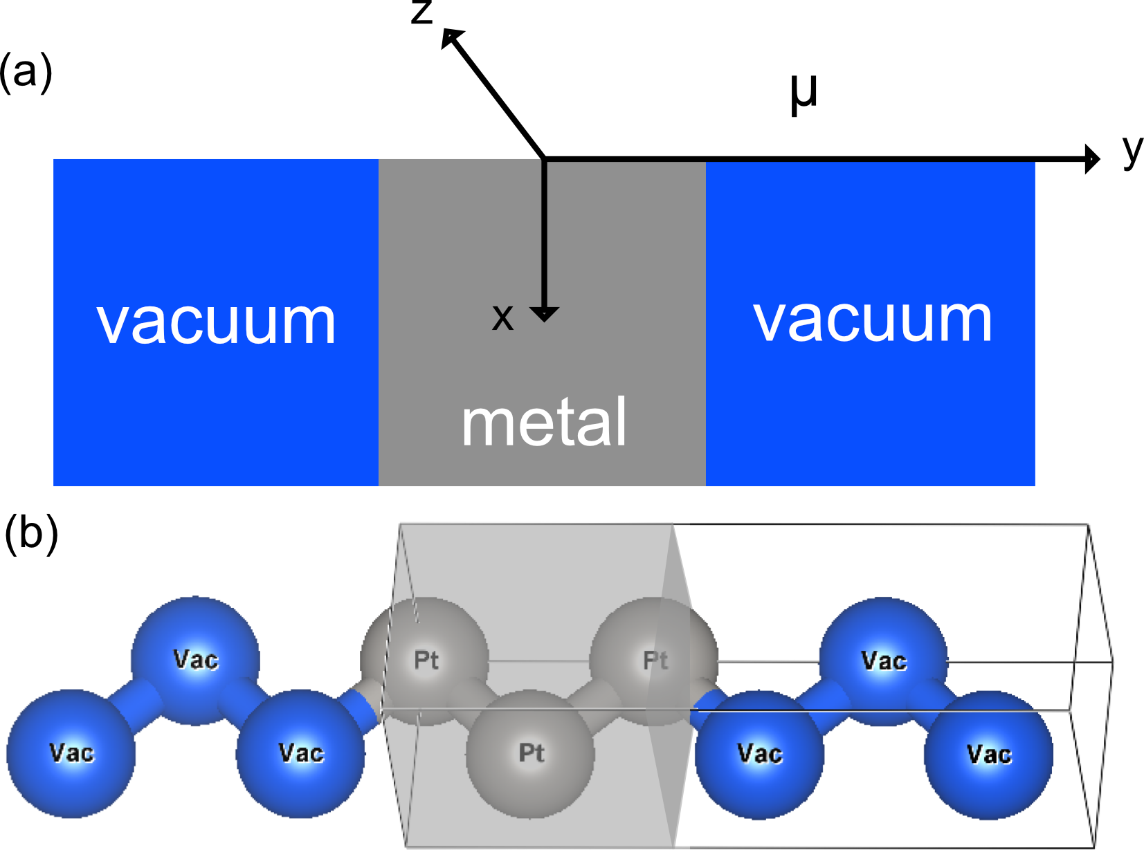
Figure 1: (a) Schematic drawing of the slab systems for the Keldysh formalism. The atomic index counts the atoms along the $y$ direction. (b) Actual unit cell for fcc Pt. For the Keldysh formalism the box indicates the supercell.
For the Boltzmann formalism the vacuum is extended into the semi-infinite half spaces on both sides of the slab (not shown).

II Theory

The electronic structure is calculated via a fully relativistic Korringa-Kohn-Rostoker (KKR) density functional theory method Zabloudil (2005). Both band structure methods, for the semiclassical approach Gradhand et al. (2009, 2010b) and the Keldysh formalism Heiliger et al. (2008); Franz et al. (2013); Mahr et al. (2017), have been introduced earlier. Here, we only highlight the adjustments and relevant expressions used to express the steady-state magnetization density.

II.1 Keldysh formalism

For the Keldysh formalism the system is divided into three parts, Left (L), Center (C) and Right (R) region. The left and right parts work as semi infinite leads. The leads are considered to be in an equilibrium state. Their influence to the center region is accounted for by the corresponding self energies $\Sigma_{L/R}$. The Fermi levels $E_{F}$ are the same, if they are of the same material. When applying a bias voltage, the levels of the chemical potential change to $\eta_{>/<}=E_{F}\pm\frac{e\Delta\varphi}{2}$ accordingly. In the range of $[\eta_{<},\eta_{>}]$ the fully relativistic electron density and magnetization density is calculated asZabloudil (2005)

$$\rho(\vec{r}) =\frac{1}{2\pi}\int_{\eta_{<}}^{\eta_{>}}\Bra{\vec{r}}\mathrm{Tr}\left[G(E)\Gamma(E)G^{\dagger}(E)\right]\Ket{\vec{r}}\;\mathrm{d}E\ \text{,}$$ (1)

$$m^{(i)}(\vec{r}) =\frac{\mu_{B}}{2\pi}\int_{\eta_{<}}^{\eta_{>}}\Bra{\vec{r}}\mathrm{Tr}\left[\beta\varsigma_{i}G(E)\Gamma(E)G^{\dagger}(E)\right]\Ket{\vec{r}}\;\mathrm{d}E\ \text{,}$$ (2)

respectively. Here, $G(E)$ is the Green’s function of the center area, and $\Gamma=i(\Sigma(E)-\Sigma^{\dagger}(E))$ the broadening function, where $\Sigma(E)=\Sigma_{L}(E)+\Sigma_{R}(E)$,

$$\beta=\begin{pmatrix}I_{2}&0\\ 0&-I_{2}\end{pmatrix},\quad\varsigma_{i}=\begin{pmatrix}\sigma_{i}&0\\ 0&\sigma_{i}\end{pmatrix},$$

$I_{2}$ is the $2\times 2$ unity matrix, and $\sigma_{i}$ are the Pauli spin matrices with $i\in\{x,y,z\}$. In the so-called one-shot calculations only the magnetization at the Fermi level is considered for vanishing bias voltage, that is

$$m_{i}(\vec{r})=\frac{\mu_{B}}{2\pi}\mathrm{Tr}[\beta\varsigma_{i}G(E_{\text{F}})\Gamma(E_{\text{F}})G^{\dagger}(E_{\text{F}})]e\Delta\varphi\ \text{.}$$

Finally, the magnetic moment due to spin accumulation $a_{x}(\mu)$ is evaluated by integrating $m_{x}(\vec{r})$ over the volume $V_{\mu}$ of the atomic sphere at atomic index $\mu$:

$$a_{x}(\mu)=\int_{V_{\mu}}m_{x}(\vec{r})\;\mathrm{d}V.$$ (3)

The current density is calculated via the Landauer-Büttiker formula in the case of a vanishing bias voltageDatta (1995)

$$j_{z}=\frac{e^{2}}{A\hbar}T(E_{\text{F}})\Delta\varphi$$ (4)

assuming the transmission $T(E)=\mathrm{Tr}[\Gamma_{L}G\Gamma_{R}G^{\dagger}]$ is nearly constant in the range of $\Delta E=e\Delta\varphi$. Here, $A$ is the area of the super cell in $x$ and $y$ direction.

II.2 Boltzmann formalism

Within the Boltzmann formalism the spin accumulation is expressed as Fermi surface integral Géranton et al. (2016). For 2D systems the spin accumulation is expressed as Herschbach et al. (2012)

$$\vec{a}=\underline{\chi}_{\mu}\cdot\vec{E}=-\frac{e\mu_{\text{B}}}{\hbar}\frac{V}{d(2\pi)^{2}}\int_{E_{\text{F}}}\frac{\mathrm{d}l}{|\vec{v}_{\vec{k}}|}\left(\vec{s}_{\vec{k}}(\mu)\circ\tau_{\vec{k}}\vec{v}_{\vec{k}}\right)\cdot\vec{E}\ \text{,}$$ (5)

where $V$ is the volume of the cell, $d$ the thickness of the film, $v_{\vec{k}}$ the group velocity at $\vec{k}$, $\vec{s}_{\vec{k}}$ the expectation value of the spin operator, and $\vec{E}$ the applied electric field. Because of degenerate states, the spin operator exhibits off-diagonal elements. A gauge transformation is applied, such that these off-diagonal elements vanish. The current density is given by

$$\vec{j}=\underline{\sigma}\cdot\vec{E}=-\frac{e^{2}}{\hbar}\frac{1}{d(2\pi)^{2}}\int_{E_{\text{F}}}\frac{\mathrm{d}l}{|\vec{v}_{\vec{k}}|}\left(\vec{v}_{\vec{k}}\circ\tau_{\vec{k}}\vec{v}_{\vec{k}}\right)\cdot\vec{E}\ \text{.}$$ (6)

Importantly both scale linearly with the relaxation time. In the chosen geometry $\vec{j}=j\vec{e}_{z}$ and $\vec{E}=E_{z}\vec{e}_{z}$, and by using the relaxation time approximation $\tau_{\vec{k}}=\tau$, the relevant expressions can be simplified as

$$a_{x}(\mu)=\chi_{xz}E_{z}=\frac{e}{\hbar}\frac{\mu_{\text{B}}V\tau E_{z}}{d(2\pi)^{2}}\int_{E_{\text{F}}}\frac{\mathrm{d}l}{|\vec{v}_{\vec{k}}|}s_{x,\vec{k}}(\mu)v_{z,\vec{k}}$$ (7)

and

$$j_{z}=\frac{e^{2}}{\hbar}\frac{\tau E_{z}}{d(2\pi)^{2}}\int_{E_{\text{F}}}\frac{v_{z,\vec{k}}v_{z,\vec{k}}}{|\vec{v}_{\vec{k}}|}\mathrm{d}l=\frac{e^{2}}{\hbar}\frac{\tau E_{z}}{d(2\pi)^{2}}\langle v_{z}^{2}\rangle.$$ (8)

This manoeuvre will allow us to remove the direct dependence of the spin accumulation on the relaxation time $\tau E_{z}$ replacing it with the current density

$$\frac{a_{x}(\mu)}{\mu_{\text{B}}}=\frac{j_{z}}{e}\frac{V}{\langle v_{z}^{2}\rangle}\int_{E_{\text{F}}}\frac{\mathrm{d}l}{|\vec{v}_{\vec{k}}|}s_{x,\vec{k}}(\mu)v_{z,\vec{k}}\ \text{.}$$ (9)

Thus the spin accumulation will scale linearly with the current density which in turn can be calculated within the Keldysh formalism. This will allow for direct mapping between the two methods.

II.3 Computational details

Slight differences in the two implementations lead to differences in the geometrical construction. For the Keldysh formalism the starting point are self-consistently calculated equilibrium potentials, which are obtained in a super cell approach including atomic spheres and vacuum spheres to form the thin film geometry. For the transport calculations, the super cell is connected to semi-infinite leads from the left and right side along the transport direction ($z$-direction). The corresponding cells are schematically shown in Fig. 1. In the following, a one-step non-equilibrium Keldysh formalism at the Fermi energy is used to find the steady-state densities from these potentials. The applied voltage is chosen reasonably small at $\Delta\varphi=10^{-4}\leavevmode\nobreak\ \textrm{Ry}/e$, in order to agree with the approximation of vanishing applied electric field in the linear response regime as assumed in the Boltzmann approach. The transmission function as well as the magnetization density does not change significantly in the small bias window.

For the Boltzmann formalism the construction is based on a slab calculation with semi-infinite vacuum attached perpendicular to the film. After obtaining the self-consistent potentials, the Fermi surface parameters such as the $\vec{k}$-resolved band velocities and spin expectation values are calculated to find the spin accumulation according to Eq. (9). Given the linear scaling of the spin accumulation with the current density in the Boltzmann formalism we insert the current density found within the Keldysh approach to facilitate direct comparison.

As a note of caution we would like to highlight the differences between the two approaches with respect to the origin of charge resistivities. Within the Landauer-Büttiker approach the finite conductance stems from a contact resistance at the interfaces of the leads. This contact resistance is also often referred to as Sharvin resistance Sharvin (1965). Naturally, it does not depend on the length of the transport system but only on the number of available transport channels. In contrast, for the Boltzmann approach the contact resistance is ignored and the whole resistance originates from scattering in the volume. In our comparison we adjust $j$ such that it fits the Sharvin resistance of the Landauer-Büttiker approach. As such the mechanism for the finite currents is different in both approaches, however the resulting current density itself is the same, driving the spin accumulation at the surfaces.

Here, we considered cubic systems (fcc and bcc). As we apply a bias in $z$ direction, the only relevant element of the spin accumulation is $a_{x}(\mu)$ and for convenience we are going to omit the index $x$ in the following. The axes of the coordinate systems are aligned parallel to the $\langle 100\rangle$ axes of the crystals.

III Results and Discussion

The resulting spin accumulation $a(\mu)$ as a function of the atomic position index $\mu$ is exemplary shown in Fig. 2 for the (a) fcc (Cu, Pt) and (b) bcc (Ta and U) systems comparing the Keldysh (K) and Boltzmann (B) formalism, respectively. The position index is chosen such that the central atom of the film is labelled as 0.

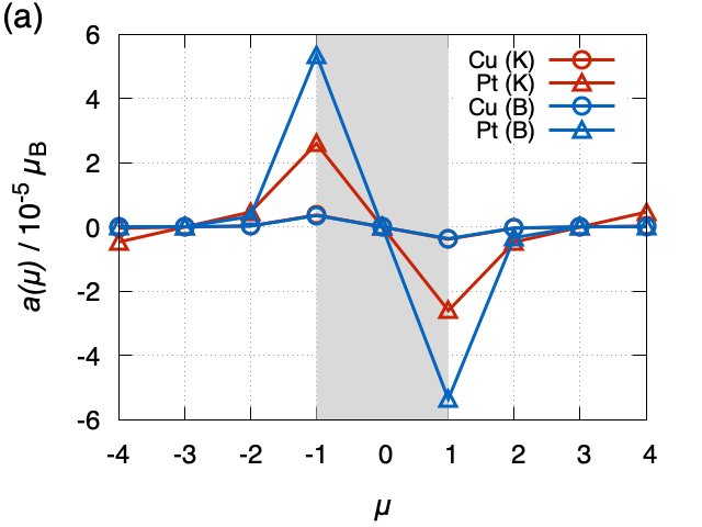
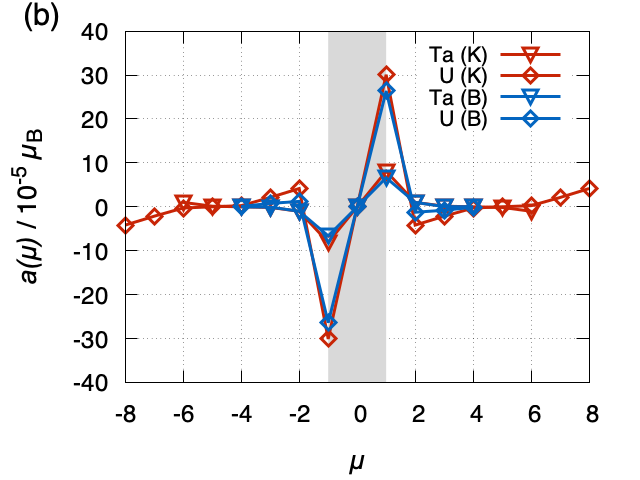
Figure 2: Plot of the magnetic moment per atom for representative (a) fcc systems and (b) bcc systems. Blue refers to Keldysh (K) calculated values, red to Boltzmann (B) calculated values. The thin film is highlighted in grey. Each line shows the same antisymmetric behaviour. Note, that in (a) the Keldysh and Boltzmann values for Cu overlap.

The general behaviour of the accumulation $a(\mu)$ in Fig. 2 is the same for all considered elements as well as between the two methods. This is largely enforced by symmetry since atoms $\mu=\pm 1$ have equal and opposite spin accumulation leading to vanishing magnetization for the central atom. For easier comparison we summarize the maximum spin accumulation $a(\mu=-1)$ for the various systems as well as the two methods in Table 1. As expected, the spin accumulation increases with increasing atomic weight corresponding to enhanced spin-orbit coupling. While this is true in general with U showing the largest effect it is not correct in the details. The spin accumulation for Ag is smaller than for Cu and for Ta we find a surprisingly large spin accumulation. Such details would be difficult to predict from simplified models. Comparing the Boltzmann to the Keldysh formalism the agreement is perfect for the noble metals, with their simple Fermi surfaces, but starts to deviate for the more complex systems Ta, Pd, Pt, and U. Nevertheless, the sign as well as the overall magnitude is still in remarkable agreement.

Table 1: First Extrema of the spin accumulation calculated by Boltzmann and Keldysh formalisms as well as the Keldysh current density for the small systems. Comparison between $a/j$ and spin Hall angle $\theta_{\text{SH}}^{\text{exp}}$Wang et al. (2014). Intrinsic spin Hall conductivities from calculations are shown for reference.

element	$a(\mu=-1)\;[10^{-6}\mu_{B}]$		$j$ $[10^{12}\text{A}\text{m}^{-2}]$	$a/j\;[10^{-17}\mu_{B}\text{m}^{2}/\text{A}]$		$\theta^{\text{exp}}_{\text{SH}}$Wang et al. (2014)	$\sigma^{\text{theo}}_{\text{SH}}$
	Boltzmann	Keldysh		Boltzmann	Keldysh	$[\%]$	$[(\hbar/e)\leavevmode\nobreak\ \Omega^{-1}\text{cm}^{-1}]$
Cu (fcc)	$3.60$	$3.77$	$1.50$	$0.24$	$0.25$	$0.32$	$-$
Ag (fcc)	$2.65$	$2.41$	$1.16$	$0.23$	$0.21$	$0.68$	$-$
Au (fcc)	$17.62$	$16.33$	$1.33$	$1.32$	$1.23$	$8.4$	$400\cite[cite]{\@@bibref{Authors Phrase1YearPhrase2}{guoInitioCalculationIntrinsic2009}{\@@citephrase{(}}{\@@citephrase{)}}}$
Ta (bcc)	$-66.19$	$-80.99$	$1.17$	$-5.66$	$-6.92$	$-7.1$	$-142\cite[cite]{\@@bibref{Authors Phrase1YearPhrase2}{qiaoCalculationIntrinsicSpin2018}{\@@citephrase{(}}{\@@citephrase{)}}}$
Pd (fcc)	$31.33$	$10.10$	$1.12$	$2.80$	$0.90$	$-$	$1400\cite[cite]{\@@bibref{Authors Phrase1YearPhrase2}{guoInitioCalculationIntrinsic2009}{\@@citephrase{(}}{\@@citephrase{)}}}$
Pt (fcc)	$53.53$	$25.99$	$1.79$	$2.99$	$1.45$	$10.00$	$2000\cite[cite]{\@@bibref{Authors Phrase1YearPhrase2}{guoIntrinsicSpinHall2008}{\@@citephrase{(}}{\@@citephrase{)}}}$
U (bcc)	$-263.9$	$-300.9$	$1.93$	$-13.7$	$-15.6$	$-$	$-402\cite[cite]{\@@bibref{Authors Phrase1YearPhrase2}{wuSpindependentTransportUranium2020}{\@@citephrase{(}}{\@@citephrase{)}}}$

We believe this correlation between Fermi surface complexity (see Fig. 5 in the Supplemental Material) and agreement between the two methods not to be a simple numerical artefact. In the Keldysh formalism we only consider the ballistic transport where each band contributes equally to the electronic transport. In contrast, the Boltzmann formalism relies on electron scattering and the weighting in any Fermi surface integral will depend on the $\vec{k}$-dependent band velocity in transport direction. For more complex structures the variations of the absolute value of the band velocity on the Fermi surface are much more pronounced (Ta, U, Pd, Pt) than for the simple metals Au, Ag, and Cu (see Fig. 5 in Supplemental Material Note (1)). As the Keldysh formalism considers the ballistic limit, entirely ignoring any scattering, the results can be interpreted as the clean limit. For elements with simple Fermi surfaces and subsequently least changing Fermi velocity, the results obtained within the Boltzmann formalism nevertheless match well. Considering they are computationally much faster they can serve as a quick alternative to the cumbersome full non-equilibrium Keldysh formalism.

So far we considered rather thin layers with limited access to the decay length of the spin accumulation within the thin film. To investigate this point further we consider three larger systems, Cu, Pt, and U, with nine layers of atoms (c.f. Fig. 3 and Supplemental MaterialNote (1)). For Cu the decay of the spin accumulation is remarkably strong, happening within 3 layers and is in excellent agreement between the two methods. In contrast, the decay appears much slower for Pt and even more so for U (see Fig. 3 (c) in Supplemental MaterialNote (1) ) again consistent between the two methods.

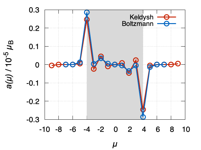
Figure 3: Magnetization for a thin film of 9 Cu atoms (highlighted in grey). While the overall behaviour is the same in both methods there are differences in the absolute values. With the Boltzmann method one gets higher values on the first peak but lower values on the second peak compared to the Keldysh method.

In order to validate our results we compare to recent experiments, where the spin accumulation of Pt thin films was directly measured by MOKE Stamm et al. (2017). In that experiment a strong thickness dependence was established with a value of $a/j=5\times 10^{-16}\leavevmode\nobreak\ \mu_{B}\text{A}^{-1}\text{m}^{2}$ for samples with a thickness $t>40\leavevmode\nobreak\ \text{nm}$. Extrapolating the experimental data (Eq. 1 in Ref. Stamm et al., 2017) to the film thickness of $t=0.39\leavevmode\nobreak\ \text{nm}$ considered here, yields a result of $a/j=1.05\times 10^{-17}\leavevmode\nobreak\ \mu_{B}\text{A}^{-1}\text{m}^{2}$ in rather good agreement to our result $a/j=1.45\times 10^{-17}\leavevmode\nobreak\ \mu_{B}\text{A}^{-1}\text{m}^{2}$. While measurements of spin Hall angles and spin Hall conductivities are widely available, to our knowledge, such direct numerical measurements of the spin accumulation for other systems are very sparse. It is therefore difficult to compare the results from our methods directly to literature values. It appears natural to compare to spin Hall conductivities or spin Hall angles predicted theoretically or measured experimentally. However, this holds multiple caveats. For example, theoretically predicted intrinsic conductivities are bulk calculations ignoring the fact that any spin accumulation will depend on the actual surface geometry and film thickness. While sign changes and over all magnitudes ought to be in agreement significant variations are possible in the details. As summarized in Table 1 the signs are in agreement between the spin accumulations and the intrinsic spin Hall conductivities but the high spin accumulation for Ta and U cannot trivially be predicted from the conductivities. On the other hand experimental results for the spin Hall angles tend to vary significantly over the various experimental techniques and sample preparations, which will often involve varying degrees of extrinsic mechanisms contributing to the overall effect.Sagasta et al. (2016) Consequently any comparison should focus on one technique with similar sample preparation only. Choosing a spin pumping experiment, in which most of the considered metals were investigated under similar conditions Wang et al. (2014) the trend for $a/j$ and $\theta_{\text{SH}}^{\text{exp}}$ in Table 1 is quite consistent for systems with simpler Fermi surfaces (Cu, Ag, Au). Similarly, Ta, Au, and Pt show increasing spin Hall angles in the same order of magnitude, with a sign change occurring for Ta.

IV Conclusion

We extended existing theoretical frameworks to capture the spin Hall effect induced spin accumulation in various metallic thin films via a fully non-equilibrium Keldysh formalism. We tested this new approach against a linearized Boltzmann approach as well as experimental findings and found remarkable agreement in all cases, reproducing all sign changes and predicting the same trends. Where the two theoretical approaches differ most is the atom resolved spin accumulation in thicker films especially for systems with complex Fermi surfaces whereas for Cu we find an excellent agreement. This new methodology will enable us to make more direct contact with experiments where instead of the conductivities derived from periodic crystals it is the spin accumulation at interfaces and surfaces as well as the spin current through interfaces which are the relevant driving mechanisms of for example magnetisation reversal in ferromagnets. In this first and most important step we have established that the developed methodology reproduces the spin Hall induced spin accumulation in the thin metallic films well across different frameworks and in comparison to experiment. This will open up broad opportunities to explore the effect in more complex interfaces as well as under the influence of impurities making even more direct contact with experimental realities. Incorporating, inversion asymmetry and contributions even under spatial inversion symmetry Freimuth et al. (2014); Wimmer et al. (2016) will give access to spin galvanic effects Skinner et al. (2015) while investigating the additional influence of impurities and the additional Mott scattering Ködderitzsch et al. (2015). In all those cases, the full non-equilibrium description adds additional complexity with the possibility of finite bias across the sample geometry.

V Acknowledgements

A. F., M. C. and C. H. acknowledge computational resources provided by the HPC Core Facility and the HRZ of the Justus-Liebig-University Giessen. Further, they would like to thank Marcel Giar and Philipp Risius of HPC-Hessen, funded by the State Ministry of Higher Education, Research and the Arts, for technical support. M.-H. W., H. R. and M. G. carried out their computational work using the computational facilities of the Advanced Computing Research Centre, University of Bristol. M.G. thanks the visiting professorship program of the Centre for Dynamics and Topology at Johannes Gutenberg-University Mainz.

References

- Dyakonov and Perel (1971) M. I. Dyakonov and V. I. Perel, Phys. Lett. A 35, 459 (1971).
- Hirsch (1999) J. E. Hirsch, Phys. Rev. B 83, 1834 (1999).
- Kato et al. (2004) Y. K. Kato, R. C. Myers, A. C. Gossard, and D. D. Awschalom, Science 306, 1910 (2004).
- Wunderlich et al. (2005) J. Wunderlich, B. Kaestner, J. Sinova, and T. Jungwirth, Phys. Rev. Lett. 94, 047204 (2005).
- Fukami et al. (2016) S. Fukami, T. Anekawa, C. Zhang, and H. Ohno, Nat. Nanotechnol. 11, 621 (2016).
- Pershin et al. (2009) Y. V. Pershin, N. A. Sinitsyn, A. Kogan, A. Saxena, and D. L. Smith, Appl. Phys. Lett. 95, 022114 (2009).
- Hoffmann (2013) A. Hoffmann, IEEE Trans. Magn. 49, 5172 (2013).
- Liu et al. (2012) L. Liu, C.-F. Pai, Y. Li, H. W. Tseng, D. C. Ralph, and R. A. Buhrman, Science 336, 555 (2012).
- Kajiwara et al. (2010) Y. Kajiwara, K. Harii, S. Takahashi, J. Ohe, K. Uchida, M. Mizuguchi, H. Umezawa, H. Kawai, K. Ando, K. Takanashi, S. Maekawa, and E. Saitoh, Nature 464, 262 (2010).
- Nakayama et al. (2013) H. Nakayama, M. Althammer, Y.-T. Chen, K. Uchida, Y. Kajiwara, D. Kikuchi, T. Ohtani, S. Geprägs, M. Opel, S. Takahashi, R. Gross, G. E. W. Bauer, S. T. B. Goennenwein, and E. Saitoh, Phys. Rev. Lett. 110, 206601 (2013).
- Wu et al. (2016) H. Wu, X. Zhang, C. H. Wan, B. S. Tao, L. Huang, W. J. Kong, and X. F. Han, Phys. Rev. B 94, 174407 (2016).
- Ando et al. (2008) K. Ando, S. Takahashi, K. Harii, K. Sasage, J. Ieda, S. Maekawa, and E. Saitoh, Phys. Rev. Lett. 101, 036601 (2008).
- Valenzuela and Tinkham (2006) S. O. Valenzuela and M. Tinkham, Nature 442, 176 (2006).
- Zhao et al. (2006) H. Zhao, E. J. Loren, H. M. van Driel, and A. L. Smirl, Phys. Rev. Lett. 96, 246601 (2006).
- Saitoh et al. (2006) E. Saitoh, M. Ueda, H. Miyajima, and G. Tatara, Appl. Phys. Lett. 88, 182509 (2006).
- Sinova et al. (2004) J. Sinova, D. Culcer, Q. Niu, N. A. Sinitsyn, T. Jungwirth, and A. H. MacDonald, Phys. Rev. Lett. 92, 126603 (2004).
- Guo et al. (2008) G. Y. Guo, S. Murakami, T.-W. Chen, and N. Nagaosa, Phys. Rev. Lett. 100, 096401 (2008).
- Murakami (2003) S. Murakami, Science 301, 1348 (2003).
- Sinova et al. (2015) J. Sinova, S. O. Valenzuela, J. Wunderlich, C. H. Back, and T. Jungwirth, Rev. Mod. Phys. 87, 1213 (2015).
- Smit (1955) J. Smit, Physica 21, 877 (1955).
- Smit (1958) J. Smit, Physica 24, 39 (1958).
- Berger (1970) L. Berger, Phys. Rev. B 2, 4559 (1970).
- Karplus and Luttinger (1954) R. Karplus and J. M. Luttinger, Phys. Rev. 95, 1154 (1954).
- Jungwirth et al. (2002) T. Jungwirth, Q. Niu, and A. H. MacDonald, Phys. Rev. Lett. 88, 207208 (2002).
- Swihart et al. (1986) J. C. Swihart, W. H. Butler, G. M. Stocks, D. M. Nicholson, and R. C. Ward, Phys. Rev. Lett. 57, 1181 (1986).
- Zahn et al. (2003) P. Zahn, J. Binder, and I. Mertig, Phys. Rev. B 68, 100403 (2003).
- Gradhand et al. (2010a) M. Gradhand, D. V. Fedorov, P. Zahn, and I. Mertig, Phys. Rev. Lett. 104, 186403 (2010a).
- Guo et al. (2005) G. Y. Guo, Y. Yao, and Q. Niu, Phys. Rev. Lett. 94, 226601 (2005).
- Yao and Fang (2005) Y. Yao and Z. Fang, Phys. Rev. Lett. 95, 156601 (2005).
- Lowitzer et al. (2011) S. Lowitzer, M. Gradhand, D. Ködderitzsch, D. V. Fedorov, I. Mertig, and H. Ebert, Phys. Rev. Lett. 106, 056601 (2011).
- Guo (2009) G. Y. Guo, J. Appl. Phys. 105, 07C701 (2009).
- Wang et al. (2006) X. Wang, J. R. Yates, I. Souza, and D. Vanderbilt, Phys. Rev. B 74, 195118 (2006).
- Yao et al. (2004) Y. Yao, L. Kleinman, A. H. MacDonald, J. Sinova, T. Jungwirth, D.-s. Wang, E. Wang, and Q. Niu, Phys. Rev. Lett. 92, 037204 (2004).
- Stamm et al. (2017) C. Stamm, C. Murer, M. Berritta, J. Feng, M. Gabureac, P. M. Oppeneer, and P. Gambardella, Phys. Rev. Lett. 119, 087203 (2017).
- Zhang (2000) S. Zhang, Phys. Rev. Lett. 85, 393 (2000).
- Freimuth et al. (2014) F. Freimuth, S. Blügel, and Y. Mokrousov, Phys. Rev. B 90, 174423 (2014).
- Wimmer et al. (2016) S. Wimmer, K. Chadova, M. Seemann, D. Ködderitzsch, and H. Ebert, Phys. Rev. B 94, 054415 (2016).
- Géranton et al. (2016) G. Géranton, B. Zimmermann, N. H. Long, P. Mavropoulos, S. Blügel, F. Freimuth, and Y. Mokrousov, Phys. Rev. B 93, 224420 (2016).
- Ködderitzsch et al. (2015) D. Ködderitzsch, K. Chadova, and H. Ebert, Phys. Rev. B 92, 184415 (2015).
- Kosma et al. (2020) A. Kosma, P. Rüßmann, S. Blügel, and P. Mavropoulos, Phys. Rev. B 102, 144424 (2020).
- Yang et al. (2016) M. Yang, K. Cai, H. Ju, K. W. Edmonds, G. Yang, S. Liu, B. Li, B. Zhang, Y. Sheng, S. Wang, Y. Ji, and K. Wang, Sci. Rep. 6, 20778 (2016).
- Avci et al. (2014) C. O. Avci, K. Garello, C. Nistor, S. Godey, B. Ballesteros, A. Mugarza, A. Barla, M. Valvidares, E. Pellegrin, A. Ghosh, I. M. Miron, O. Boulle, S. Auffret, G. Gaudin, and P. Gambardella, Phys. Rev. B 89, 214419 (2014).
- Nikolić et al. (2005) B. K. Nikolić, S. Souma, L. P. Zârbo, and J. Sinova, Phys. Rev. Lett. 95, 046601 (2005), arXiv:cond-mat/0412595 .
- Nikolic et al. (2006) B. K. Nikolic, L. P. Zarbo, and S. Souma, Phys. Rev. B 73, 075303 (2006), arXiv:cond-mat/0506588 .
- Zabloudil (2005) J. Zabloudil, ed., Electron Scattering in Solid Matter: A Theoretical and Computational Treatise, Springer Series in Solid-State Sciences No. 147 (Springer, Berlin ; New York, 2005).
- Gradhand et al. (2009) M. Gradhand, M. Czerner, D. V. Fedorov, P. Zahn, B. Y. Yavorsky, L. Szunyogh, and I. Mertig, Phys. Rev. B 80, 224413 (2009).
- Gradhand et al. (2010b) M. Gradhand, D. V. Fedorov, P. Zahn, and I. Mertig, Phys. Rev. B 81, 020403 (2010b).
- Heiliger et al. (2008) C. Heiliger, M. Czerner, B. Y. Yavorsky, I. Mertig, and M. D. Stiles, J. Appl. Phys. 103, 07A709 (2008).
- Franz et al. (2013) C. Franz, M. Czerner, and C. Heiliger, J. Phys. Condens. Matter 25, 425301 (2013).
- Mahr et al. (2017) C. E. Mahr, M. Czerner, and C. Heiliger, Phys. Rev. B 96, 165121 (2017).
- Datta (1995) S. Datta, Electronic Transport in Mesoscopic Systems (Cambridge University Press, 1995).
- Herschbach et al. (2012) C. Herschbach, M. Gradhand, D. V. Fedorov, and I. Mertig, Phys. Rev. B 85, 195133 (2012).
- Sharvin (1965) Y. V. Sharvin, Zh. Eksperim. i Teor. Fiz. 48, 984 (1965).
- Wang et al. (2014) H. L. Wang, C. H. Du, Y. Pu, R. Adur, P. C. Hammel, and F. Y. Yang, Phys. Rev. Lett. 112, 197201 (2014).
- Qiao et al. (2018) J. Qiao, J. Zhou, Z. Yuan, and W. Zhao, Phys. Rev. B 98, 214402 (2018).
- Wu et al. (2020) M.-H. Wu, H. Rossignol, and M. Gradhand, Phys. Rev. B 101, 224411 (2020).
- Note (1) Supplemental Material.
- Sagasta et al. (2016) E. Sagasta, Y. Omori, M. Isasa, M. Gradhand, L. E. Hueso, Y. Niimi, Y. Otani, and F. Casanova, Phys. Rev. B 94, 060412 (2016).
- Skinner et al. (2015) T. D. Skinner, K. Olejník, L. K. Cunningham, H. Kurebayashi, R. P. Campion, B. L. Gallagher, T. Jungwirth, and A. J. Ferguson, Nat. Commun. 6, 6730 (2015).