Effectively Counting $s-t$ Simple Paths in Directed Graphs

Abstract

An important tool in analyzing complex social and information networks is $s-t$ simple path counting, which is known to be $\#$P-complete. In this paper, we study efficient $s-t$ simple path counting in directed graphs. For a given pair of vertices $s$ and $t$ in a directed graph, first we propose a pruning technique that can efficiently and considerably reduce the search space. Then, we discuss how this technique can be adjusted with exact and approximate algorithms, to improve their efficiency. In the end, by performing extensive experiments over several networks from different domains, we show high empirical efficiency of our proposed technique. Our algorithm is not a competitor of existing methods, rather, it is a friend that can be used as a fast pre-processing step, before applying any existing algorithm.

Keywords

Complex network analysis; directed graphs; simple paths; $s-t$ (simple) path counting; exact algorithm; approximate algorithm.

1 Introduction

Graphs (networks) are powerful tools that are used to model data in different domains, including social networks, information networks, road networks and the world wide web. A property seen in most of these real-world networks is that the links between the vertices do not always represent reciprocal relations [18]. Consequently, the generated networks are directed graphs, where any edge has a direction and the edges are not necessarily symmetric.

Path counting is an important problem in analyzing large networks. For example, some of network indices, such as $k$-path centrality are based on counting paths [7]. A computationally demanding path counting problem is $s-t$ simple path counting. In this problem, given two vertices $s$ and $t$, the goal is to count the number of all simple paths from $s$ to $t$. A simple path is path that contains each node of the graph at most once. For both directed and undirected graphs, this problem is known to be $\#$P-complete [25]. Hence, it is critical to develop algorithms that work efficiently in practice.

In this paper, we focus on efficient $s-t$ simple path counting in directed graphs. Our key contributions are as follows.

• First, for a given pair of vertices $s$ and $t$, we propose a pruning technique that can reduce the search space significantly. Moreover, it can be computed very efficiently.

• Then, we discuss how this technique can be adjusted with exact and approximate algorithms, to improve their performance. We show, for example, that under some conditions, applying this pruning technique yields a polynomial time exact algorithm for enumerating $s-t$ simple paths.

• Finally, by performing extensive experiments over several networks from different domains (social, peer-to-peer, communication, citation, stack exchange, product co-purchasing, …), we show high empirical efficiency of our pruning technique.

Our algorithm is not a competitor of existing $s-t$ simple path counting algorithms. Rather, it is a friend as it can be used as a fast pre-processing step, before applying any of existing algorithms.

The rest of this paper is organized as follows. In Section 2, we introduce preliminaries and necessary definitions used in the paper. In Section 3, we give an overview on related work. In Section 4, we present our pruning technique and discuss how it improves exact and approximate algorithms. In Section 5, we empirically evaluate our pruning technique. Finally, the paper is concluded in Section 6.

2 Preliminaries

We assume that the reader is familiar with basic concepts in graph theory. Throughout the paper, $G$ refers to a directed graph. For simplicity, we assume that $G$ is a connected and loop-free graph without multi-edges. By default, we assume that $G$ is an unweighted graph, unless it is explicitly mentioned that $G$ is weighted. $V(G)$ and $E(G)$ refer to the set of vertices and the set of edges of $G$, respectively. For a vertex $v\in V(G)$, the number of head ends adjacent to $v$ is called its in degree and the number of tail ends adjacent to $v$ is called its out degree. For a vertex $v$, by $\mathcal{ON}_{G}(v)$ we denote the set of outgoing neighbors of $v$ in the graph $G$. A (directed) walk in a directed graph is a sequence of edges directed in the same direction and joins a sequence of vertices. A directed trail is a (directed) walk wherein all the edges are distinct. A (simple and directed) path is a (directed) trail wherein all the vertices are distinct. Let $A\subset V(G)$. The subgraph of $G$ induced by $A$ is the graph whose vertices are $A$ and edges are all the edges in $E(G)$ that have both endpoints in $A$.

3 Related work

There exist a number of algorithms in the literature for counting/enumerating/listing $s-t$ simple paths. In one of the earlier studies, Valiant [25] showed that it is $\#$P-complete to enumerate simple $s-t$ paths in both directed and undirected graphs. In [10], Hura utilized Petri nets to enumerate all $s-t$ simple paths in a directed graph. Bax [2] exploited Hamiltonian path algorithms to derive an $O\left(2^{|V(G)|}poly(|V(G)|)\right)$ time and $O\left(poly(|V(G)|)\right)$ space algorithm for $s-t$ simple path counting. Knuth [11] presented the simpath algorithm that generates a (not-always-reduced) binary decision diagram for all simple paths from $s$ to $t$. The constructed diagram is called zero-suppressed decision diagram (ZDD). In recent years, more efficient algorithms have been proposed to construct ZDD [26]. Roberts and Kroese [22] presented an approximate algorithm for $s-t$ simple path counting, which is based on sequential importance sampling (we discuss their algorithm in more details in Section 4.3, and explain how our pruning technique can improve it). In [17], Mihalák et.al. studied approximately counting approximately shortest paths in directed graphs. However, their algorithm is restricted to directed acyclic graphs (DAGs).

In the literature, there are problems that are close to our studied problem, or are a restricted form of it. In the following, we briefly review them:

• In a restricted form of our studied problem, the number of $s-t$ simple paths of a (fixed) length $l$ are counted. Flum and Grohe [8] proved that counting simple paths of length $l$ on both directed and undirected graphs, parameterized by $l$, is #W[1]-complete. Recently, Giscard et.al. [9] proposed an algorithm for counting $s-t$ simple paths of length up to $l$. Time complexity of their algorithm is $O\left(|V(G)|+|E(G)|+(l^{w}+l\Delta)|S_{l}|\right)$, where $\Delta$ is the maximum degree of the graph, $|S_{l}|$ is the number of weakly connected induced subgraphs of $G$ on at most $l$ vertices, and $w$ is the exponent of matrix multiplication.

• The other problem which is close to our studied problem is counting the number of all paths from a vertex $s$ to another vertex $t$. However, unlike our studied problem (which is $\#$P-complete), this problem can be solved in polynomial time, using e.g., dynamic programming or fast matrix multiplication. For example and as described in e.g., [3], the number of all paths of size $k$ (simple or non-simple) from $s$ to $t$ is equal to the $st$-th entry of $A^{k}$, where $A$ is the adjacency matrix of the graph and $A^{k}$ is the $k$-th power of $A$. Arenas et.al. [1] study the problem of counting the number of all paths between two vertices $s$ and $t$ of a length at most $k$, and show that it admits a fully polynomial-time randomized approximation scheme (FPRAS).

• Another relevant problem is counting the number of shortest paths between a given pair of vertices. Unlike our studied problem, this problem can be solved efficiently in polynomial time, too. Using breadth first search (BFS), this problem can be solved in $O\left(|V(G)|+|E(G)|\right)$ time [3]. Recently, a number of faster approximate algorithms have been proposed to address this problem in static [16] and dynamic graphs [24]. The notion of shortest paths is used to develop several tools of network analysis, including betweenness centrality [4, 6, 5].

In the current paper, we propose a pruning technique to improve exact/approximate algorithms of the general form of $s-t$ simple path counting in directed graphs. Our algorithm is not a competitor of these existing algorithms. Rather, it is a friend that can be used as a fast pre-processing step before applying any of them.

4 Counting $s-t$ paths in directed graphs

In this section, given a source vertex $s$ and a target vertex $t$ in a directed graph $G$, we propose algorithms to count the number of all simple paths from $s$ to $t$. First in Section 4.1, we present a pruning technique used to reduce search space for $s-t$ path counting. Then in Section 4.2, we discuss how this pruning technique improves exact $s-t$ path counting. Finally in Section 4.3, we study how our pruning technique can improve approximate algorithms.

4.1 A pruning technique

In this section, we describe our pruning technique. We start with introducing the sets $\mathcal{S}_{st}$ (Definition 1) and $\mathcal{IS}_{ts}$ (Definition 3), that are used to reduce the search space.

Definition 1.

Let $G$ be a directed graph and $s,t,v\in V(G)$ such that $s\neq t$. We say $v$ is in the scope of $s$ with respect to $t$ iff either $v=s$, or there is at least one directed path from $s$ to $v$ in $G$ that does not pass over $t$. The set of vertices $v$ that are in the scope of $s$ with respect to $t$ is denoted with $\mathcal{S}_{st}$.

Definition 2.

Let $G$ be a directed graph. Inverse graph of $G$, denoted with $\mathcal{I}(G)$, is a directed graph such that: (i) $V(\mathcal{I}(G))=V(G)$, and (ii) $(u,v)\in E(\mathcal{I}(G))$ if and only if $(v,u)\in E(G)$ [6].

Definition 3.

Let $G$ be a directed graph and $s,t,v\in V(G)$ such that $s\neq t$. We say $v$ is inversely in the scope of $t$ with respect to $s$ iff either $v=t$, or there is at least one directed path from $t$ to $v$ in $\mathcal{I}(G)$ that does not pass over $s$ . The set of vertices $v$ that are inversely in the scope of $t$ with respect to $s$ is denoted with $\mathcal{IS}_{ts}$.

For example, in the graph of Figure 1, $\mathcal{S}_{st}$ consists of vertices $s$, $v_{1}$, $v_{2}$, $v_{3}$, $v_{4}$, $v_{5}$ and $t$. It does not contain vertex $v_{6}$, as the path from $s$ to $v_{6}$ passes over $t$. Moreover, $\mathcal{IS}_{ts}$ consists of vertices $t$, $v_{5}$ and $s$. For a given pair of vertices $s,t\in V(G)$, we can compute $\mathcal{S}_{st}$ and $\mathcal{IS}_{ts}$ efficiently in $O(|E(G)|)$ time. To compute $\mathcal{S}_{st}$, we act as follows:

1. First, if $G$ is weighted, weights of the edges of $G$ are discarded,

2. Then, a (revised) breadth first search (BFS) or a depth-first search (DFS) on $G$ starting from $s$ is conducted, with an small change: when $t$ is met, the traversal is not expanded to the children (and descendants) of $t$. All the vertices that are met during the traversal are appended to $\mathcal{S}_{st}$.

To compute $\mathcal{IS}_{ts}$, we act as follows:

1. First, by flipping the direction of the edges of $G$, we construct $\mathcal{I}(G)$,

2. Then, if $G$ is weighted, weights of the edges are discarded,

3. Finally, a (revised) breadth-first search or depth-first search on $\mathcal{I}(G)$ starting from $t$ is conducted, with an small change: when $s$ is met, the traversal is not expanded to its children (and descendants). All the vertices that are met during the traversal are appended to $\mathcal{IS}_{ts}$.

It is easy to see that both $\mathcal{S}_{st}$ and $\mathcal{IS}_{ts}$ can be computed in $O(|E(G)|)$ time, for both unweighted and weighted graphs. Furthermore, we have the following lemma.

Lemma 1.

Given a directed graph $G$ and vertices $s,t\in V(G)$, the number of simple paths from $s$ to $t$ is equal to the number of simple paths from $s$ to $t$ whose vertices belong to $\mathcal{S}_{st}\cap\mathcal{IS}_{ts}$.

Proof.

Each path should start from $s$ and end with $t$, therefore its vertices should belong to both $\mathcal{S}_{st}$ and $\mathcal{IS}_{ts}$. ∎

Lemma 1 says that in order to compute $s-t$ paths, we require to consider only those paths that their vertices belong to both $\mathcal{S}_{st}$ and $\mathcal{IS}_{ts}$. We can use this to prune many vertices of the graph that do not belong to either $\mathcal{S}_{st}$ or $\mathcal{IS}_{ts}$ or both. As a result, if in a graph, $\mathcal{S}_{st}\cap\mathcal{IS}_{ts}$ is (considerably) smaller than the number of vertices of the graph, this pruning technique can enormously improve the efficiency of the $s-t$ path counting algorithm. Note that time complexity of $s-t$ simple path counting algorithms is exponential in terms of the number of vertices of the graph. Hence, discarding a considerable part of the vertices can hugely improve the efficiency of the algorithms.

In Algorithm 1, we use this optimization technique to make $s-t$ path counting algorithms more efficient. If $out\_degree$ of $s$ is $0$ or $in\_degree$ of $t$ is $0$, there is no path from $s$ to $t$, hence, Algorithm 1 returns $0$. Then, it computes $\mathcal{S}_{st}$ and $\mathcal{IS}_{ts}$ and stores them respectively in the sets $S$ and $IS$. Then, for each vertex $v$ in the graph, we check if it belongs to both $S$ and $IS$. We form the subgraph induced by all such vertices and call it $\rho_{st}(G)$. Finally, we apply the $s-t$ path counting algorithm on $\rho_{st}(G)$. the graph $\rho_{st}(G)$ is usually much smaller than $G$, therefore, the algorithm can be run much faster.

Figure 1: The graph on left is a directed graph $G$ and the graph on right shows $\rho_{st}(G)$. Over $G$ and $s$ and $t$, while the variance of our algorithm is $0$, the variance of the algorithm of [22] is $4$.

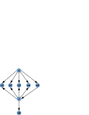
(a) A graph $G$

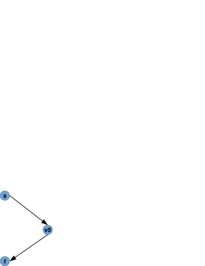
(b) $\rho_{st}(G)$

Algorithm 1 High level pseudo code of computing the number of $s-t$ paths in a directed graph.

1:  Input. A directed network $G$, a pair of vertices $s,t\in V(G)$.

2:  Output. The number of simple paths from $s$ to $t$.

3:  if out degree of $s$ is $0$ or in degree of $t$ is $0$ then

4:     return  $0$.

5:  end if

6:  $S\leftarrow$ compute $\mathcal{S}_{st}$.

7:  $IS\leftarrow$ compute $\mathcal{IS}_{ts}$.

8:  for all vertices $v\in V(G)$ do

9:     if $v\in S$ and $v\in IS$ then

10:        Mark $v$.

11:     end if

12:  end for

13:  $\rho_{st}(G)\leftarrow$ the induced subgraph of $G$ consisting of the marked vertices.

14:  $path\_no\leftarrow$ call an (exact/approximate) $s-t$ path counting algorithm on $\rho_{st}(G)$.

15:  return  $path\_no$.

4.2 Exact algorithm

In an exact algorithm for counting $s-t$ simple paths that exhaustively enumerates all simple paths from $s$ to $t$, we can use backtracking: we start from $s$, take a path and walk it (so that the path does not contain repeated vertices). If the path ends to $t$, we count it and backtrack and take some other path. If the path does not reach to $t$, we discard it and take some other path. This algorithm enumerates all the paths from $s$ to $t$. We refer to this algorithm as Exhaustive Simple Path Enumerator, or ESPE in short. As discussed in [25], enumerating $s-t$ paths for both directed and undirected graphs is $\#$P-complete. In the following, we discuss that using our pruning technique and for a certain type of vertices in a directed graph, the simple path enumeration problem can be solved in polynomial time.

In the $s-t$ simple path counting problem, the input size consists of the number of vertices and the number of edges of $G$. In Theorem 1 we show that if for $s$ and $t$, $\left|\mathcal{S}_{st}\cap\mathcal{IS}_{ts}\right|$ is a constant, then the $s-t$ simple counting problem can be solved efficiently. Later in Section 5 we empirically show that in most of real-world networks, vertices $s$ and $t$ have usually a small quantity for $\left|\mathcal{S}_{st}\cap\mathcal{IS}_{ts}\right|$. It should be highlighted that even for such pairs of vertices, applying the above mentioned exhaustive simple path enumeration algorithm without using our pruning technique, does not yield a polynomial time algorithm.

Theorem 1.

Let $G$ be a directed graph, where for a given pair of vertices $s$ and $t$, $|V\left(\rho_{st}(G)\right)|)$ is a constant. The list of simple paths from $s$ to $t$ can be enumerated in polynomial time (in terms of $|V(G)|$ and $|E(G)|$).

Proof.

We can compute the sets $\mathcal{S}_{st}$, $\mathcal{IS}_{ts}$, and their intersection in $O(|E(G)|)$ time. So, $\rho_{st}(G)$ can be computed in $O(|E(G)|)$ time. After that, we work with $\rho_{st}(G)$ which has only a constant number of vertices. Hence, all the paths can be enumerated in a constant time. ∎

In fact, the proof of Theorem 1 presents a much better result than polynomial time: it says that under the mentioned condition and after a linear time spent to construct $\rho_{st}(G)$, the whole list can be enumerated in a constant time (in terms of $|V(G)|$ and $|E(G)|$).

4.3 Approximate algorithm

Roberts and Kroese [22] proposed randomized algorithms for estimating the number of $s-t$ simple paths in a graph. In this section, we investigate how the first randomized algorithm of [22] can be improved using our pruning technique . First, we briefly describe how this algorithm changes if we apply our pruning technique on it. Then, we analyze this revised algorithm and compare it with the first algorithm of [22].

In the approximate algorithm, we sample $N$ independent (random) paths and compute the probability of sampling each path. The following procedure is used to sample each path:

1. Start with vertex $s$. Initialize the following variables: $c\leftarrow s$ (current vertex), $h\leftarrow 1$ (probability), $k\leftarrow 1$ (counter), and $p\leftarrow\{s\}$ (path).

2. Mark $s$ as $visited$ (to be sure that $p$ will not visit $s$ again).

3. Let $V^{\prime}=\{v\in\mathcal{ON}_{\rho_{st}(G)}(c)|v\text{ is not }visited\}$ be the set of possible vertices for the next step of the path.

4. Choose the next vertex $v\in V^{\prime}$ of the path uniformly at random and set $x_{k+1}$ to $v$.

5. Set $c\leftarrow v$, $h\leftarrow\frac{h}{|V^{\prime}|}$, $k\leftarrow k+1$, and $p\leftarrow p\cup\{v\}$. Mark $v$ as $visited$.

6. If $c=t$, then stop. Otherwise go to step $3$.

If we do not use our pruning technique, instead of working with $\rho(G)$, we should work (e.g., in step 3) with $G$. This has consequences. For example, while a path sampled from $G$ may never reach to $t$ (so after some iterations, $V^{\prime}$ becomes empty), this never happens when we work with $\rho(G)$. Hence, as stated in [22], when working with $G$ we need to check the following condition in step 3: if $V^{\prime}=\emptyset$, we do not generate a valid path, so stop.

Let $x_{1},x_{2},\ldots,x_{m}$ be the set of vertices of each path $p$, with $x_{1}=s$. In the above mentioned procedure, path $p$ is chosen with probability:

$$h(p)= h(x_{2}|x_{1})\cdot h(x_{3}|x_{1},x_{2})\ldots h(x_{m}|x_{1},\ldots,x_{m-1})$$

$$= \left|\mathcal{ON}_{\rho_{st}(G)}(x_{1})\setminus\{x_{1}\}\right|\cdot\left|\mathcal{ON}_{\rho_{st}(G)}(x_{2})\setminus\{x_{1},x_{2}\}\right|\ldots$$

$$\left|\mathcal{ON}_{\rho_{st}(G)}(x_{m-1})\setminus\{x_{1},\ldots,x_{m-1}\}\right|$$ (1)

Let $\mathcal{X}$ be the set of simple paths from $s$ to $t$. Let also $p^{1},\ldots,p^{N}$ be the set of sampled paths. For each $p^{k}$, we estimate the number of $s-t$ simple paths as $X^{k}=\frac{1}{h(p^{k})}$. The final estimation is the average of estimations of different samples:

$$X=\frac{1}{N}\sum_{k=1}^{N}\frac{1}{h(p^{k})}.$$ (2)

It is easy to see that $X$ is an unbiased estimator for the number of simple paths from $s$ to $t$:

$$\mathbb{E}[X^{k}]=\sum_{p\in\mathcal{X}}\frac{1}{h(p)}\cdot h(p)=\sum_{p\in\mathcal{X}}1=|\mathcal{X}|.$$

Since $X$ is the average of $N$ random variables whose expected values is $|\mathcal{X}|$, the expected value of $X$ is $|\mathcal{X}|$, too.

For the variance of $X$, we have:

$$\mathbb{V}ar\left[X^{k}\right] =\mathbb{E}\left[(X^{k})^{2}\right]-\mathbb{E}\left[X^{k}\right]^{2}$$

$$=\sum_{p\in\mathcal{X}}\frac{1}{h(p)^{2}}\cdot h(p)-\mathcal{X}^{2}=\sum_{p\in\mathcal{X}}\frac{1}{h(p)}-\mathcal{X}^{2}.$$

Since $X$ is the average of $N$ independent random variable $X^{1},\ldots,X^{N}$, we have:

$$\mathbb{V}ar\left[X\right]=\frac{1}{N}\sum_{p\in\mathcal{X}}\frac{1}{h(p)}-\frac{\mathcal{X}^{2}}{N}.$$

Now let compare this variance with the variance of the estimator of the algorithm of [22]. Unlike our algorithm, in the algorithm of [22] it is possible that a sampled path does not belong to $\mathcal{X}$. Let $\mathbf{X}$ be the sample space of the algorithm of [22] that consists of those paths in $G$ that start from $s$ and end to $t$ or to a vertex whose $V^{\prime}$ is empty. In a way similar to our analysis, its variance is:

$$\mathbb{V}ar\left[X\right] =\frac{1}{N}\sum_{p\in\mathbf{X}}\frac{I(p\in\mathbf{X})}{h^{\prime}(p)}-\frac{\mathcal{X}^{2}}{N}$$

$$=\frac{1}{N}\sum_{p:p\in\mathcal{X}}\frac{1}{h^{\prime}(p)}-\frac{\mathcal{X}^{2}}{N},$$ (3)

where $h^{\prime}(p)$ is defined as follows ($x_{1},\ldots,x_{m}$ are vertices of $p$):

$$h^{\prime}(p)= \left|\mathcal{ON}_{G}(x_{1})\setminus\{x_{1}\}\right|\cdot\left|\mathcal{ON}_{G}(x_{2})\setminus\{x_{1},x_{2}\}\right|\ldots$$

$$\left|\mathcal{ON}_{G}(x_{m-1})\setminus\{x_{1},\ldots,x_{m-1}\}\right|.$$ (4)

Moreover in Equation 4.3, $I(p\in\mathcal{X})$ is an indicator function, which is $1$ if $p$ is a path from $s$ to $t$, and $0$ otherwise.

Comparing Equation 4.3 with Equation 4.3 reveals that our algorithm has a better (lower) variable. In order to have a lower variance, an algorithm should assign as low as possible probabilities to the paths that it may sample but they do not belong to $\mathcal{X}$. Because in this case their inverse will be a very large number and the contribution of these large numbers to the variance will be $0$. Our algorithm assigns probability $0$ to such paths, so it manages them very efficiently. However, the algorithm of [22] may assign a (large) non-zero value to many of them. For example, in Figure 1 assume that we want to estimate the number of simple paths from vertex $s$ to vertex $t$. The sample space of our algorithm consists of only only one path which is the path $s\rightarrow v_{5}\rightarrow t$. Hence, the variance of its estimation, even when $N$ is $1$, is $0$. In contrast, the sample space of the algorithm of [22] consists of $5$ paths: $s\rightarrow v_{1}$, $s\rightarrow v_{2}$, $s\rightarrow v_{3}$, $s\rightarrow v_{4}$, and $s\rightarrow v_{5}\rightarrow t$, where it assigns an equal probability $1/5$ to each path. Among them, only the last one belongs to $\mathcal{X}$. While this algorithm assigns the same probability to each one, our algorithm gives probability $0$ to the paths that do not belong to $\mathcal{X}$. With $N=1$, the variance of the estimation of the algorithm of [22] is $4$. Since our algorithm assigns probability $0$ to the paths that are not in $\mathcal{X}$, it never finds a variance worse than the algorithm of [22].

Table 1: Specifications of our large networks.

Dataset	#vertices	#edges	domain
soc-sign-Slashdot090221 [13]	82140	549202	social
soc-sign-epinions [13]	131828	841372	social
p2p-Gnutella08 [15]	6301	20777	peer-to-peer file sharing
p2p-Gnutella30 [15]	36682	88328	peer-to-peer file sharing
p2p-Gnutella31 [15]	62586	147892	peer-to-peer file sharing
wikiVote [13]	7115	103689	Wikipedia vote
collegeMsg [19]	1899	59835	message exchanging
soc-Epinions1 [21]	75879	508837	who-trust-whom
email-EuAll [15]	265214	420045	communication
cit-HepPh [14]	34546	421578	citation
cit-HepTh [14]	27770	352807	citation
sx-mathoverflow [20]	24818	506550	stack exchange (Math Overflow)
sx-askubuntu [20]	159316	964437	stack exchange (Ask Ubuntu)
sx-superuser [20]	194085	1443339	stack exchange (Super User)
amazon0302 [12]	262111	1234877	product co-purchasing
amazon0312 [12]	400727	3200440	product co-purchasing

5 Experimental results

In order to evaluate the empirical behaviour of our pruning technique, we perform extensive experiments over several real-world networks from different domains. The objective is to empirically show that in real-world directed networks, for a given pair of vertices $s$ and $t$, $\mathcal{S}_{st}\cap\mathcal{IS}_{ts}$ is small (compared to $V(G)$), and it can be computed very efficiently. These two automatically improve efficiency of any (exact/approximate) simple path counting algorithm.

Table 2: Empirical evaluation of our proposed pruning technique. Column $max_{sz}$ presents the maximum size of $\mathcal{S}_{st}\cap\mathcal{IS}_{ts}$ divided by the number of vertices (over different pairs of $s,t$ vertices). Column $max_{tm}$ presents the maximum time to compute $\mathcal{S}_{st}\cap\mathcal{IS}_{ts}$, where the reported times are in second(s).

Dataset	$max_{sz}$	$max_{tm}$
soc-sign-Slashdot090221	0.3333	0.0889
soc-sign-epinions	0.3144	0.1172
p2p-Gnutella08	0.3296	0.0014
p2p-Gnutella31	0.2261	0.0150
p2p-Gnutella30	0.2315	0.0081
wikiVote	0.1570	0.0068
collegeMsg	0.6821	0.0004
email-EuAll	0.1289	0.0618
soc-Epinions1	0.4246	0.0761
cit-HepPh	0.0000002	0.2833
cit-HepTh	0.0000002	0.2765
sx-mathoverflow	0.1478	0.0495
sx-askubuntu	0.1160	0.1399
sx-superuser	0.1477	0.2418
amazon0302	0.9229	0.2255
amazon0312	0.9488	0.5525

Table 3: Specifications of our smaller networks.

Dataset	#vertices	#edges	domain
bio-CE-GN [23]	2220	53683	Gene functional associations
bio-SC-LC [23]	2004	20452	Gene functional associations
bn-mouse_retina_1 [23]	1123	90811	Brain network
C1000-9 [23]	1001	450081	DIMACS
C2000-9 [23]	2001	1799534	DIMACS
SmaGri [23]	1060	4921	Citation network

Table 4: Empirical comparison of our proposed pruning technique. All the reported times are in seconds and ”not terminated” means the algorithm does not terminate within 12 hours!

Dataset	max $\left|\mathcal{S}\cap\mathcal{IS}\right|$	max total running time		max $\#$simple paths
		pruned-ESPE	ESPE
bio-CE-GN	135	5.253	not terminated	1,180,840
bio-SC-LC	144	414.605	not terminated	119,738,817
bn-mouse_retina_1	29	183.987	not terminated	17,012,976
C1000-9	35	195.333	448.225	919,343,373
C2000-9	34	171.182	253.073	887,306,870
SmaGri	52	0.001	5.973	1,030

The experiments are done on an Intel processor clocked at $2.4$ GHz with $3$ GB main memory, running Ubuntu Linux $18.04.2$ LTS. We perform our tests over 16 real-world datasets from the SNAP repository. The specifications of the datasets are summarized in Table 1. Over each dataset, we choose $500$ pairs of vertices $s$ and $t$, uniformly at random. Then, we run our proposed pruning technique for each pair. In the end, we report maximum size of $\mathcal{S}_{st}\cap\mathcal{IS}_{ts}$ divided by $|V(G)|$ (in the $max_{sz}$ column) and the maximum time to compute $\mathcal{S}_{st}\cap\mathcal{IS}_{ts}$ (in the $max_{tm}$ column), over all the sampled pairs.

The results are reported in Table 2. On the one hand, since $max_{sz}$ is usually considerably smaller than the number of vertices of the graph, our pruning technique usually makes the real-world graphs considerably smaller. Hence, any $s-t$ path counting problem (exact, approximate, …) can be solved much faster on the smaller graph. Compared to the number of vertices, we may consider $\mathcal{S}_{st}\cap\mathcal{IS}_{ts}$ as a constant. Therefore after pruning, the $s-t$ path counting algorithm finds a constant time. Note that the reported values for $|\mathcal{S}_{st}\cap\mathcal{IS}_{ts}|/|V(G)|$ are the maximum ones and most of the other values are much smaller.

On the other hand, the values reported in the $max_{tm}$ column indicate that computing $\mathcal{I}_{st}$, $\mathcal{IS}_{ts}$, and their intersection can be done very quickly. Note that $max_{tm}$ contains all the time required to compute $\mathcal{S}_{st}$, $\mathcal{IS}_{ts}$, and their intersection. As reported in the table, over all the datasets, $max_{tm}$ is less than $0.6$ seconds! This time is quite ignorable, compared to the time of counting all $s-t$ simple paths. Note that while worst case time complexity of our pruning technique is $O(|E(G)|)$, in practice it is usually performed much faster. The reason is that for most of vertices, the direction of edges makes the sets $\mathcal{S}$ and $\mathcal{IS}$ small. As a result, BFSs (or DFSs) conducted on these small sets, can be conducted very efficiently.

In our experiments, we tried to compare the ESPE algorithm (discussed in Section 4.2), against the method wherein first we apply our pruning technique and then we use ESPE (we refer to this method as pruned-ESPE). However, over any of the above mentioned networks, none of the methods ESPE and pruned-ESPE finish during a reasonable time (24 hours!). Therefore and to compare the efficiency of pruned-ESPE against ESPE, we switch to smaller graphs. Our smaller real-world graphs have between 1K-2.3K vertices. Their specifications are summarized in Table 3 (they can be downloaded from http://networkrepository.com/networks.php). We treat all these networks as directed graphs.

When comparing pruned-ESPE against ESPE, we perform the following scenario: over each dataset, we sample uniformly at random 500 pairs of nodes $s$ and $t$, such that there exists at least one path from $s$ to $t$. Then for each pair, we run pruned-ESPE and ESPE and compute the following statistics: $\left|\mathcal{S}\cap\mathcal{IS}\right|$, total running time of pruned-ESPE (which includes the pre-processing/pruning phase), running time of ESPE, and the number of simple paths. In the end and among all the sampled pairs, we choose the pair that yields the maximum number of simple paths and report the results of this chosen pair. For both algorithms, this chosen pair usually takes the most amount of time to process. Thus, ”max $\left|\mathcal{S}\cap\mathcal{IS}\right|$” depicts the value of $\left|\mathcal{S}\cap\mathcal{IS}\right|$ for the chosen pair, ”max total running time” depicts the total time to process the chosen pair (by each of the algorithms), and ”max #simple paths” presents the number of simple paths between the two nodes of the chosen pair.

Table 4 reports the results. As seen in the table, using our proposed pruning techniques significantly improves the running time. All the times reported in this table are in seconds, and ”not terminated” means the algorithm does not terminate within 12 hours! So, for the chosen pair and over bio-CE-GN, bio-SC-LC and bn-mouseretina1, while ESPE doe not produce the results during a reasonable time (12 hours!), pruned-ESPE processes the chosen pairs quickly. Over the other graphs that both algorithms terminate within a reasonable time, pruned-ESPE acts quite faster. As evidenced by the values of the ”max $\left|\mathcal{S}\cap\mathcal{IS}\right|$” column, this is due to the efficiency of our pruning technique in considerably reducing the search space.

6 Conclusion

In this paper, we studied efficient $s-t$ simple path counting in directed graphs. For a given pair of vertices $s$ and $t$ in a directed graph, first we presented a pruning technique that can efficiently reduce the search space. Then, we investigated how this pruning technique can be adjusted with exact and approximate algorithms, to improve their efficiency. In the end, we performed extensive experiments over several real-world networks to show the empirical efficiency of our proposed pruning technique.

References

- [1] Marcelo Arenas, Luis Alberto Croquevielle, Rajesh Jayaram, and Cristian Riveros. Efficient logspace classes for enumeration, counting, and uniform generation. In Dan Suciu, Sebastian Skritek, and Christoph Koch, editors, Proceedings of the 38th ACM SIGMOD-SIGACT-SIGAI Symposium on Principles of Database Systems, PODS 2019, Amsterdam, The Netherlands, June 30 - July 5, 2019, pages 59–73. ACM, 2019.
- [2] Eric T. Bax. Algorithms to count paths and cycles. Inf. Process. Lett., 52(5):249–252, 1994.
- [3] U. Brandes. A faster algorithm for betweenness centrality. Journal of Mathematical Sociology, 25(2):163–177, 2001.
- [4] Mostafa Haghir Chehreghani. An efficient algorithm for approximate betweenness centrality computation. Comput. J., 57(9):1371–1382, 2014.
- [5] Mostafa Haghir Chehreghani, Talel Abdessalem, and Albert Bifet. Metropolis-hastings algorithms for estimating betweenness centrality. In Melanie Herschel, Helena Galhardas, Berthold Reinwald, Irini Fundulaki, Carsten Binnig, and Zoi Kaoudi, editors, Advances in Database Technology - 22nd International Conference on Extending Database Technology, EDBT 2019, Lisbon, Portugal, March 26-29, 2019, pages 686–689. OpenProceedings.org, 2019.
- [6] Mostafa Haghir Chehreghani, Albert Bifet, and Talel Abdessalem. Efficient exact and approximate algorithms for computing betweenness centrality in directed graphs. In 22nd Pacific-Asia Conference on Knowledge Discovery and Data Mining, PAKDD, 2018.
- [7] Mostafa Haghir Chehreghani, Albert Bifet, and Talel Abdessalem. Adaptive algorithms for estimating betweenness and k-path centralities. In Wenwu Zhu, Dacheng Tao, Xueqi Cheng, Peng Cui, Elke A. Rundensteiner, David Carmel, Qi He, and Jeffrey Xu Yu, editors, Proceedings of the 28th ACM International Conference on Information and Knowledge Management, CIKM 2019, Beijing, China, November 3-7, 2019, pages 1231–1240. ACM, 2019.
- [8] Jörg Flum and Martin Grohe. The parameterized complexity of counting problems. SIAM J. Comput., 33(4):892–922, 2004.
- [9] Pierre-Louis Giscard, Nils M. Kriege, and Richard C. Wilson. A general purpose algorithm for counting simple cycles and simple paths of any length. Algorithmica, 81(7):2716–2737, 2019.
- [10] G.S. Hura. Enumeration of all simple paths in a directed graph using petri net: A systematic approach. Microelectronics Reliability, 23(1):157 – 159, 1983.
- [11] Donald Knuth. The Art of Computer Programming, volume 4A. Addison-Wesley Professional, Boston, MA, USA, 2011.
- [12] Jure Leskovec, Lada A. Adamic, and Bernardo A. Huberman. The dynamics of viral marketing. ACM Transactions on the Web (TWEB), 1(1), 2007.
- [13] Jure Leskovec, Daniel P. Huttenlocher, and Jon M. Kleinberg. Signed networks in social media. In Proceedings of the 28th International Conference on Human Factors in Computing Systems, Atlanta, Georgia, USA, April 10-15, pages 1361–1370, 2010.
- [14] Jure Leskovec, Jon M. Kleinberg, and Christos Faloutsos. Graphs over time: densification laws, shrinking diameters and possible explanations. In Robert Grossman, Roberto J. Bayardo, and Kristin P. Bennett, editors, Proceedings of the Eleventh ACM SIGKDD International Conference on Knowledge Discovery and Data Mining, Chicago, Illinois, USA, August 21-24, 2005, pages 177–187. ACM, 2005.
- [15] Jure Leskovec, Jon M. Kleinberg, and Christos Faloutsos. Graph evolution: Densification and shrinking diameters. ACM Transactions on Knowledge Discovery from Data (TKDD), 1(1), 2007.
- [16] Dennis Nii Ayeh Mensah, Hui Gao, and Liang Wei Yang. Approximation algorithm for shortest path in large social networks. Algorithms, 13(2):36, 2020.
- [17] Matús Mihalák, Rastislav Srámek, and Peter Widmayer. Approximately counting approximately-shortest paths in directed acyclic graphs. Theory Comput. Syst., 58(1):45–59, 2016.
- [18] M. E. J. Newman. The structure and function of complex networks. SIAM REVIEW, 45:167–256, 2003.
- [19] Pietro Panzarasa, Tore Opsahl, and Kathleen M. Carley. Patterns and dynamics of users’ behavior and interaction: Network analysis of an online community. JASIST, 60(5):911–932, 2009.
- [20] Ashwin Paranjape, Austin R. Benson, and Jure Leskovec. Motifs in temporal networks. In Maarten de Rijke, Milad Shokouhi, Andrew Tomkins, and Min Zhang, editors, Proceedings of the Tenth ACM International Conference on Web Search and Data Mining, WSDM 2017, Cambridge, United Kingdom, February 6-10, 2017, pages 601–610. ACM, 2017.
- [21] Matthew Richardson, Rakesh Agrawal, and Pedro M. Domingos. Trust management for the semantic web. In Dieter Fensel, Katia P. Sycara, and John Mylopoulos, editors, The Semantic Web - ISWC 2003, Second International Semantic Web Conference, Sanibel Island, FL, USA, October 20-23, 2003, Proceedings, volume 2870 of Lecture Notes in Computer Science, pages 351–368. Springer, 2003.
- [22] Ben Roberts and Dirk P. Kroese. Estimating the number of s-t paths in a graph. J. Graph Algorithms Appl., 11(1):195–214, 2007.
- [23] Ryan A. Rossi and Nesreen K. Ahmed. The network data repository with interactive graph analytics and visualization. In Blai Bonet and Sven Koenig, editors, Proceedings of the Twenty-Ninth AAAI Conference on Artificial Intelligence, January 25-30, 2015, Austin, Texas, USA, pages 4292–4293. AAAI Press, 2015.
- [24] Konstantin Tretyakov, Abel Armas-Cervantes, Luciano García-Bañuelos, Jaak Vilo, and Marlon Dumas. Fast fully dynamic landmark-based estimation of shortest path distances in very large graphs. In Craig Macdonald, Iadh Ounis, and Ian Ruthven, editors, Proceedings of the 20th ACM Conference on Information and Knowledge Management, CIKM 2011, Glasgow, United Kingdom, October 24-28, 2011, pages 1785–1794. ACM, 2011.
- [25] Leslie G. Valiant. The complexity of enumeration and reliability problems. SIAM J. Comput., 8(3):410–421, 1979.
- [26] Norihito Yasuda, Teruji Sugaya, and Shin-ichi Minato. Fast compilation of s-t paths on a graph for counting and enumeration. In Antti Hyttinen, Joe Suzuki, and Brandon M. Malone, editors, Proceedings of the 3rd Workshop on Advanced Methodologies for Bayesian Networks, AMBN 2017, Kyoto, Japan, September 20-22, 2017, volume 73 of Proceedings of Machine Learning Research, pages 129–140. PMLR, 2017.