Spin effects on neutron star fundamental-mode dynamical tides:
phenomenology and comparison to numerical simulations

Abstract

Gravitational waves from neutron star binary inspirals contain information on strongly-interacting matter in unexplored, extreme regimes. Extracting this requires robust theoretical models of the signatures of matter in the gravitational-wave signals due to spin and tidal effects. In fact, spins can have a significant impact on the tidal excitation of the quasi-normal modes of a neutron star, which is not included in current state-of-the-art waveform models. We develop a simple approximate description that accounts for the Coriolis effect of spin on the tidal excitation of the neutron star’s quadrupolar and octupolar fundamental quasi-normal modes and incorporate it in the SEOBNRv4T waveform model. We show that the Coriolis effect introduces only one new interaction term in an effective action in the co-rotating frame of the star, and fix the coefficient by considering the spin-induced shift in the resonance frequencies that has been computed numerically for the mode frequencies of rotating neutron stars in the literature. We investigate the impact of relativistic corrections due to the gravitational redshift and frame-dragging effects, and identify important directions where more detailed theoretical developments are needed in the future. Comparisons of our new model to numerical relativity simulations of double neutron star and neutron star-black hole binaries show improved consistency in the agreement compared to current models used in data analysis.

I Introduction

The gravitational waves (GWs) from inspiraling binary systems encode detailed information about the nature and internal structure of the compact objects. These signatures arise from spin and tidal effects, including dynamical tides associated with the excitation of the objects’ characteristic quasi-normal modes. This is particularly interesting for neutron stars (NSs), where gravity compresses matter up to several times the normal nuclear density Lattimer and Prakash (2016); Rezzolla et al. (2018a), making NSs unique laboratories for the ground state of strongly interacting matter at the highest physically possible densities. The new opportunities for characterizing such matter with GWs were demonstrated with the first binary NS merger event GW170817  Abbott et al. (2017a, 2019, b, b); Bauswein et al. (2017); Annala et al. (2018); Most et al. (2018); Ruiz et al. (2018); Margalit and Metzger (2017); Rezzolla et al. (2018b); Shibata et al. (2017); Abbott et al. (2018, 2019); De et al. (2018); Radice et al. (2018); Coughlin et al. (2018, 2019); Dai et al. (2018); Radice and Dai (2019); Lucca and Sagunski (2020); Capano et al. (2020); Dietrich et al. (2020a); Raaijmakers et al. (2020). In the future, higher-precision GW measurements for populations of NS have the potential to advance our understanding of the fundamental physics of strong interactions as well as the emergent multibody phenomena in subatomic matter. Extracting the information on matter from GW signals from binaries is critically predicated on highly accurate theoretical waveform models that link between features in GWs and source parameters Cutler and Flanagan (1994); Veitch et al. (2015); Abbott et al. (2020). In particular, the waveform models must include all relevant physical effects. This requires a detailed understanding of the behavior of matter in spinning, relativistic objects under nonlinear, dynamical gravity, which is a challenging task.

A significant research effort in the last decades has focused on developing GW models for binary black holes (BHs), which involve only vacuum gravity and are characterized by only their masses and spins Carter (1971); Hawking (1972); Gürlebeck (2015). There has also been much recent progress on describing the effects of matter in binary inspirals. A number of studies have focused on GW signatures of dynamical tides associated with different NS modes within different approximations Bildsten and Cutler (1992); Reisenegger and Goldreich (1994); Lai et al. (1993); Lai (1994); Reisenegger and Goldreich (1994); Zahn (1977); Willems et al. (2003); Zahn (1970); Kopal (1978); Kochanek (1992); Hansen (2006); Mora and Will (2004); Kokkotas and Schaefer (1995); Flanagan and Hinderer (2008); Ferrari et al. (2012); Damour et al. (1992); Shibata (1994); Rathore et al. (2003); Lai (1994); Vines and Flanagan (2013); Vines et al. (2011); Chakrabarti et al. (2013a); Andersson and Ho (2018); Yu and Weinberg (2017); Tsang (2013); Tsang et al. (2012); Pnigouras (2019); Pratten et al. (2020a); Schmidt and Hinderer (2019); Suvorov and Kokkotas (2020); Andersson and Pnigouras (2020); Pan et al. (2020); Ng et al. (2020); Pons et al. (2002); Gualtieri et al. (2001), rotational multipole moments Krishnendu et al. (2017); Bohé et al. (2015); Marsat (2015); Levi and Steinhoff (2015a); Porto et al. (2012, 2011); Levi and Steinhoff (2015b); Buonanno et al. (2013); Levi and Teng (2021); Levi et al. (2020, 2021), gravitomagnetic tidal interactions Flanagan and Racine (2007); Favata (2006); Landry and Poisson (2015a); Pani et al. (2018); Landry and Poisson (2015b); Banihashemi and Vines (2020); Poisson (2020a, b); Poisson and Buisson (2020); Gupta et al. (2021), eccentricity Gold et al. (2012); Chirenti et al. (2017); Yang (2019); Vick and Lai (2019), nonlinear mode couplings Xu and Lai (2017); Essick et al. (2016); Landry and Poisson (2015b), spin-tidal couplings in the adiabatic limit Jiménez Forteza et al. (2018); Abdelsalhin et al. (2018); Pani et al. (2015a, b); Endlich and Penco (2016); Gagnon-Bischoff et al. (2018); Landry (2017); Landry and Poisson (2015c); Dietrich et al. (2019a); Levi et al. (2020), and the effects of spins on the tidal response of black holes Le Tiec and Casals (2020); Le Tiec et al. (2020); Chia (2020); Goldberger et al. (2020) as well as on dynamical tides in NSs in the Newtonian limit Ho and Lai (1999); Ma et al. (2020a); Lai (1999, 1997); Ivanov et al. (2015); Lai and Wu (2006); Ma et al. (2020b). Recently, effective-field-theory calculations of tidal effects in scattering events have also come into focus Kälin and Porto (2020); Kälin et al. (2020), see also Ref. Bini et al. (2020), and Refs. Cheung and Solon (2020); Haddad and Helset (2020); Cheung et al. (2021); Bern et al. (2020) for analogous work based on massive quantum fields or scattering amplitudes.

Substantial further effort has gone into developing state-of-the-art waveform models for data analysis within the so-called phenomenological IMRPhenom Ajith et al. (2007, 2008); Khan et al. (2016); Husa et al. (2016); Hannam et al. (2014); Schmidt et al. (2012, 2015); Ajith et al. (2011); Santamaria et al. (2010); Khan et al. (2020); García-Quirós et al. (2020); Dietrich et al. (2017, 2019b); Pratten et al. (2020b, c) and effective-one-body (EOB) SEOBNR/TEOBResumS families Buonanno and Damour (1999, 2000); Bohé et al. (2017); Babak et al. (2017); Taracchini et al. (2012, 2014); Pan et al. (2014a, b); Barausse and Buonanno (2010); Barausse et al. (2009); Babak et al. (2017); Barausse and Buonanno (2011); Pan et al. (2011); Cotesta et al. (2018); Ossokine et al. (2020); Nagar et al. (2019, 2018); Damour and Nagar (2014a, b); Damour et al. (2013); Damour and Nagar (2009); Damour et al. (2008a, 2009, b); Messina et al. (2018); Nagar et al. (2017); Nagar and Shah (2016); Damour (2001); Damour et al. (2008c); Nagar (2011); Balmelli and Jetzer (2013); Nagar et al. (2020, 2017); Damour and Nagar (2014b); Bernuzzi et al. (2012); Nagar and Akcay (2012); Nagar (2011) (see also the reviews Dietrich et al. (2020b); Damour and Nagar (2016, 2011); Buonanno and Sathyaprakash (2014); Damour (2014); Hannam (2014); Damour (2008)). These models all include the effects of spin-induced multipole moments and the dominant tidal effects characterized by equation-of-state-dependent tidal deformability (or Love number) coefficients. In previous work, we calculated the effects of dynamical tides from the fundamental ($f$-) modes and incorporated them in the SEOBNR models Hinderer et al. (2016); Steinhoff et al. (2016), leading e.g. to the SEOBNRv4T model. However, our model of dynamical tides had several limitations. For instance, we did not consider the effects of spin on the tidal response of the NS, which is the most prominent effect of spin-matter interactions.

In this paper, we extend the parameter space of waveform models by accounting for these spin effects in an approximate way, and investigate their role in NSNS and NSBH binaries. As expected on physical grounds and confirmed in previous work, e.g. Ho and Lai (1999); Foucart et al. (2019); Ma et al. (2020a), the effect of spins on dynamical $f$-mode tides can significantly enhance the matter signatures in GWs in the late inspiral for anti-aligned spins, depending also on the parameters. We show in this paper that this can lead to non-negligible dephasings with current data analysis models which neglect this effect. It is therefore urgent to model dynamical tides of rotating NS to enable the robustness of using GWs as probes for subatomic physics as the LIGO Aasi et al. (2015), Virgo Acernese et al. (2015), and KAGRA Akutsu et al. (2020) GW detectors are improving in sensitivity and new, third-generation facilities are being envisioned. We study three main effects that influence the orbital frequency in a binary in which a rotating NS’s $f$-mode is resonantly excited by the tidal field of the companion: (i) the gravitational redshift of the NS, (ii) the relativistic dragging of the NS’s inertial frame, including also the additional effects of the orbiting companion, and (iii) the Coriolis effect due to the NS’s spin. We derive an estimate for the resonant orbital frequency which approximately takes into account all of these effects and demonstrate that the most important effect is due to the NS’s spin because of near-cancellations between the redshift and frame-dragging effects. We develop a simple modification of the existing $f$-mode EOB waveform model which includes the Coriolis effect and is based on introducing spin-dependent shifts in the $f$-mode frequency and tidal deformability coefficients. We test our model against results from numerical relativity simulations both for aligned and anti-aligned spins and find improved consistency compared to current models used in data analysis. Our simple model can readily be used to improve GW measurements. A more detailed theoretical study and model development which also overcomes other limitations and includes dynamical tides in the odd-parity sector will be the subject of forthcoming works.

The organization of this paper is as follows. We begin in Sec. II by deriving a Newtonian action for quadrupolar, parity-even dynamical tides in rotating stars. We start from a description in terms of the normal modes for the fluid displacement due to the perturbations and convert to a basis of symmetric-tracefree tensors. That basis is more convenient for identifying selection rules, and for generalizing to relativistic stars. Such a generalization is worked out in Sec. III in the co-rotating frame where the background (unperturbed) fluid is at rest, provided we allow for general coupling coefficients not restricted to their Newtonian values. We specialize to the case of $f$-modes, which have the largest tidal couplings, and work to linear order in the rotation frequency. This leads to an effective action with one as yet undetermined coefficient characterizing the Coriolis interaction between the star’s spin and its tidal spin, i.e., the angular momentum associated with the dynamical quadrupole. In Sec. IV we extend the action to a binary system and derive explicit equations of motion within the post-Newtonian approximation for the orbital dynamics. From the solutions for the quadrupole we obtain the response function whose features we analyze in Sec. V. We discuss how to determine the spin-tidal Coriolis coefficient by matching to results for the $f$-mode frequencies of rotating neutron stars from the literature and obtain a quasi-universal relation for this shift. Next, we consider the impact of relativistic effects—gravitational redshift and frame-dragging—on the dynamical tides and quantify their importance. In Sec. VI we derive a simple phenomenological model that accounts for the Coriolis effect by applying spin-dependent shifts of the $f$-mode frequency and tidal deformability parameter in the existing SEOBNRv4T waveform model. We test this model against numerical relativity simulations of spinning binary neutron star and neutron star – black hole binaries from the BAM and SXS codes in Sec. VII. Section VIII contains our conclusions, and the Appendix contains a brief discussion of the relation of this paper to Ref. Ma et al. (2020a).

The notation here follows that in Ref. Steinhoff et al. (2016). We use geometric units with $G=c=1$ throughout. Capitalized Latin indices $A$, $B$, …on tensors denote the representation in the spatial co-rotating frame and take values 1, 2, 3. Greek letters $\mu$, $\nu$, …denote spacetime coordinate indices and run through 0, 1, 2, 3. Lower-case Latin indices $i$, $j$, …run through 1, 2, 3 and denote either spatial coordinate indices when used on position variables or indices in a local euclidean frame comoving with the center of the star for other tensors (spin, quadrupole) Levi and Steinhoff (2015a); Steinhoff et al. (2016). Boldface notation for vectors with such indices is also used. Round brackets around indices denote the symmetrization, square brackets denote the corresponding antisymmetric combination, and angle brackets denote symmetric-tracefree projection. Our convention for the Riemann tensor is

$$R^{\mu}{}_{\nu\alpha\beta}=\Gamma^{\mu}{}_{\nu\beta,\alpha}-\Gamma^{\mu}{}_{\nu\alpha,\beta}+\Gamma^{\rho}{}_{\nu\beta}\Gamma^{\mu}{}_{\rho\alpha}-\Gamma^{\rho}{}_{\nu\alpha}\Gamma^{\mu}{}_{\rho\beta},$$ (1)

where $\Gamma^{\mu}{}_{\nu\beta}$ is the Christoffel symbol. In the derivations we consider the case with only one extended body, which we label as body 1 with mass $m_{1}$. Since we work in the regime of linearized tides, the case of two stars can be obtained by adding the same contribution with the body labels exchanged. For a binary system, we define the total mass $M=m_{1}+m_{2}$, the reduced mass $\mu=m_{1}m_{2}/M$, and the symmetric mass ratio $\nu=\mu/M$.

II Newtonian dynamical tides of rotating stars

In this section we recapitulate Newtonian tides as linear perturbations of a background solution for a star in equilibrium following Refs. Chandrasekhar (1964); Steinhoff et al. (2016); Chakrabarti et al. (2013a); Flanagan and Hinderer (2008); Gupta et al. (2021) (see also, e.g., Refs. Schenk et al. (2002); Lynden-Bell and Ostriker (1967); Rathore et al. (2003)). The perturbation is described by a displacement vector field of the fluid elements ${\bm{\xi}}({\bm{x}},t)$ away from their background position. It is useful to consider the function space of all displacements as a complex Hilbert space with an inner product

$$\langle{\bm{\xi}},{\bm{\xi}}^{\prime}\rangle=\int d^{3}x\rho_{0}\,{\bm{\xi}}^{*}\!\cdot{\bm{\xi}}^{\prime},$$ (2)

where $\rho_{0}$ is the unperturbed mass density of the background configuration.

We restrict the discussion here to an ideal fluid with barotropic equation of state $\rho(p)$ relating the mass density $\rho$ and the isotropic pressure $p$. That is, we neglect effects from, e.g., temperature, viscosity, and buoyancy, which play a subdominant role for the fundamental modes in neutron stars. We will first briefly recall the non-rotating case and obtain the Lagrangian describing the dynamics of the tidal perturbations, then generalize to include effects of spin to linear order in the rotation frequency, and finally transform to a description in terms of symmetric-tracefree tensors.

II.1 Nonrotating stars

We first consider a nonrotating, hence spherically symmetric, star in equilibrium with density $\rho_{0}(r)$. The star is then placed in an external gravitational potential $\Phi$, which induces dynamical perturbations to the fluid. We will consider the perturbations only to linear order. For instance, the mass density perturbation is $\delta\!\rho=-\nabla(\rho_{0}{\bm{\xi}})$, where ${\bm{\xi}}={\bm{\xi}}^{*}$ is the physical fluid displacement. The equations of motion for the dynamical tidal perturbations can be derived from a Lagrangian for the fluid displacement given by

$$L_{\text{DT}}=\frac{1}{2}\langle\dot{{\bm{\xi}}},\dot{{\bm{\xi}}}\rangle-\frac{1}{2}\langle{\bm{\xi}},\mathcal{D}{\bm{\xi}}\rangle+\langle{\bm{f}}^{\rm ext},{\bm{\xi}}\rangle.$$ (3)

The first term in Eq. (3) is the kinetic energy of the perturbation, the second term specifies the energies associated with the internal restoring forces, while the last term is the potential energy in the external field. For the case considered in this paper, the external force is ${\bm{f}}^{\rm ext}=-\nabla\Phi$ where $\Phi$ is the gravitational potential of a binary companion orbiting at a distance ${\bm{r}}(t)$ and given by

$$\Phi=-\frac{m_{2}}{|{\bm{x}}-{\bm{r}}(t)|}.$$ (4)

The linear operator $\mathcal{D}$ is defined by

$$\mathcal{D}{\bm{\xi}}=-\nabla\left\{\left[\frac{c_{s}^{2}}{\rho_{0}}+4\pi\Delta^{-1}\right]\nabla\cdot(\rho_{0}{\bm{\xi}})\right\},$$ (5)

where $c_{s}=\sqrt{(\partial p_{0}/\partial\rho_{0})}$ is the speed of sound of the background fluid configuration with pressure $p_{0}$. The first term in Eq. (5) comes from the perturbation of the internal energy, and the second (nonlocal) term describes the gravitational self-energy of the perturbation.

The operator $\mathcal{D}$ is Hermitian with respect to the inner product (2). Thus its eigenvectors ${\bm{\xi}}_{n\ell m}$ are an orthonormal basis of the normal modes labeled by the type of mode $n$, the multipolar order $\ell$, and an angular-momentum number $m$ associated with a decomposition into (vector) spherical harmonics. The real eigenvalues $\omega_{n\ell}^{2}$, where $\omega_{n\ell}$ is the mode frequency, are determined from

$$\mathcal{D}{\bm{\xi}}_{n\ell m}=\omega_{n\ell}^{2}{\bm{\xi}}_{n\ell m},\quad\langle{\bm{\xi}}_{n\ell m},{\bm{\xi}}_{n^{\prime}\ell^{\prime}m^{\prime}}\rangle=\delta_{nn^{\prime}}\delta_{\ell\ell^{\prime}}\delta_{mm^{\prime}}.$$ (6)

The mode frequencies $\omega_{n\ell}$ are degenerate over $m$ because the operator $\mathcal{D}$ is rotation symmetric. Similarly, due to parity invariance of $\mathcal{D}$, the modes can be categorized as even parity (electric-type) or odd-parity (magnetic-type). As the integration measure $\rho_{0}d^{3}x$ of the inner product (2) has compact support, the normal modes ${\bm{\xi}}_{n\ell m}$ are countable and are enumerated by the number $n$ (besides $\ell$ and $m$). We restrict our attention to pressure modes in this paper and take $n$ to be the number of radial nodes. The fundamental pressure mode or $f$-mode is then labeled by $n=0$.

We can decompose any fluid displacement ${\bm{\xi}}$ into the orthonormal basis of the normal modes,

$${\bm{\xi}}=\sum_{n\ell m}q_{n\ell m}(t){\bm{\xi}}_{n\ell m}({\bm{x}}),\quad q_{n\ell m}=\langle{\bm{\xi}}_{n\ell m},{\bm{\xi}}\rangle,$$ (7)

with time-dependent amplitudes $q_{n\ell m}(t)$. The reality condition ${\bm{\xi}}={\bm{\xi}}^{*}$ implies that $q_{n\ell m}^{*}=(-1)^{m}q_{n\ell\,-m}$, which follows from the analogous relation for the spherical harmonics. The general Lagrangian then reads

$$L_{\text{DT}}=\sum_{n\ell m}\left[\frac{1}{2}|\dot{q}_{n\ell m}|^{2}-\frac{1}{2}\omega_{n\ell}^{2}|q_{n\ell m}|^{2}+\langle{\bm{f}}^{\rm ext},{\bm{\xi}}_{n\ell m}\rangle\,q_{n\ell m}\right].$$ (8)

To compute the coefficients for the overlap between the external field and the mode functions, and to identify the modes giving the most important contributions to $L_{\rm DT}$, it is useful to express the potential from Eq. (4) as a Taylor series expansion around the center of the star. Choosing coordinates such that the center of the star is located at ${\bm{x}}=0$, the expansion of the potential is

$$\Phi(t,{\bm{x}})=\Phi(t,{\bm{0}})+x^{j}\partial_{j}\Phi(t,{\bm{x}})|_{{\bm{x}}=0}+\sum_{\ell=2}^{\infty}\frac{1}{\ell!}x^{L}E_{L}$$ (9)

where the $\ell$-th tidal moments $E_{L}$ for $\ell\geq 2$ are defined by (following the conventions in Steinhoff et al. (2016)):

$$E_{L}=\partial_{L}\Phi\!\mid_{{\bm{x}}=0},$$ (10)

and $L=A,B,C,\ldots$ denotes a string of $\ell$ indices. Note that $E_{L}$ is symmetric and tracefree, which follows from $\Delta\Phi\!\mid_{{\bm{x}}=0}=0$. The tidal potential can equivalently be written as a spherical harmonic multipolar expansion given by

$$\Phi=-m_{2}\sum_{\ell,m}\frac{4\pi}{2\ell+1}\frac{|{\bm{x}}|^{\ell}}{r(t)^{\ell+1}}Y_{\ell m}\left(\frac{\pi}{2},\phi\right)Y_{\ell m}^{*}(\theta,\varphi),$$ (11)

where ${\bm{x}}$ and $(\theta,\varphi)$ are associated with a comoving coordinate system centered on the star, and $r,\phi$ characterize the orbital coordinates in the equatorial plane. We define the overlap integral $I_{n\ell}$ by

$$I_{n\ell}=\langle\nabla|{\bm{x}}|^{\ell}Y_{\ell m}(\theta,\varphi),{\bm{\xi}}_{n\ell m}\rangle.$$ (12)

The term $\langle{\bm{f}}^{\rm ext},{\bm{\xi}}_{n\ell m}\rangle$ in the Lagrangian can then be written as

$$\langle{\bm{f}}^{\rm ext},{\bm{\xi}}_{n\ell m}\rangle=-\frac{N_{\ell}}{\ell!}I_{n\ell}E^{*}_{\ell m},$$ (13)

where

$$E_{\ell m}=N_{\ell}\mathcal{Y}^{*\ell m}_{L}E_{L}=-(2\ell-1)!!\,N_{\ell}Y^{*}_{\ell m}\left(\frac{\pi}{2},\phi\right)\frac{m_{2}}{r^{\ell+1}}.$$ (14)

This can be either obtained from Eq. (10) or its spherical-harmonic analog Eq. (11). Recall that one can convert between spherical harmonics and unit vectors using the identity $Y_{\ell m}=\mathcal{Y}^{\ell m}_{L}n^{\langle L\rangle}$ and defining the coefficient $N_{\ell}=\sqrt{4\pi\ell!/(2\ell+1)!!}$ that arises when applying the inverse conversion to change from $n^{\langle A}n^{B\rangle}$ to $Y_{\ell m}$; see e.g. Ref. Gupta et al. (2021) for useful formulas.

The modes with the largest contributions to $L_{\rm DT}$ can be identified by the following considerations. First, we note that the $\ell$th multipole of the external tidal field associated with $\ell\geq 2$ derivatives of $\Phi$ is increasingly suppressed for increasing multipole orders $\ell$. We thus expect the dominant contributions to come from the low-$\ell$ modes. However, the $\ell=0,1$, as well as all magnetic-type modes do not couple linearly to the external gravitational field in the Newtonian case. The $\ell=0$ interaction is forbidden due to the conservation of mass, while the $\ell=1$ interaction leads to an overall motion of the star, which has no gauge-invariant physical meaning according to the weak equivalence principle (universality of free fall). The magnetic modes couple linearly to gravitomagnetic tidal fields which is a relativistic phenomenon that is absent in Newtonian gravity. Hence, to leading order, the external field drives the electric quadrupolar ($\ell=2$) modes, so we restrict our attention to them in the following.

II.1.1 Transformation to the basis of symmetric-tracefree Cartesian tensors

We can equivalently express the Lagrangian in terms of symmetric-tracefree tensors using the conversion between spherical harmonics and unit vectors provided by the symmetric-tracefree tensors ${\cal Y}^{\ell m}_{L}$. The mode amplitudes $q_{n\ell m}$ can then be directly translated to Cartesian tensors. For the quadrupole $\ell=2$, we adopt the normalization

$$Q_{n}^{AB}=\sqrt{2\lambda_{n}}\omega_{n}N_{2}\sum_{m}\mathcal{Y}_{AB}^{2m}q_{n2m},$$ (15)

where $N_{2}=\sqrt{8\pi/15}$, $\omega_{n}=\omega_{n2}$ is the mode frequency, and $\lambda_{n}$ is the tidal deformability of the mode, related here to the overlap integral by

$$\lambda_{n}=\frac{N_{2}^{2}I_{n2}^{2}}{2\omega_{n}^{2}}=\frac{4\pi I_{n2}^{2}}{15\omega_{n}^{2}}.$$ (16)

The total quadrupole is given by summing over all overtones

$$Q_{AB}=\sum_{n=0}^{\infty}Q_{n}^{AB}.$$ (17)

We also define the Newtonian quadrupolar tidal tensor

$$E^{AB}=\partial_{A}\partial_{B}\Phi({\bm{x}})\mid_{{\bm{x}}=0}.$$ (18)

The Lagrangian (8) can then be written as

$$L_{\text{DT}}=\sum_{n}\bigg{[}\frac{1}{4\lambda_{n}\omega_{n}^{2}}\left(\dot{Q}_{n}^{AB}\dot{Q}_{n}^{AB}-\omega_{n}^{2}Q_{n}^{AB}Q_{n}^{AB}\right)\\ -\frac{1}{2}E^{AB}Q_{n}^{AB}\bigg{]}.$$ (19)

We remind the reader that $Q_{n}^{AB}$ is the contribution of the $n$-mode to the (symmetric-tracefree) quadrupole of the star, and $E^{AB}$ is the external tidal field evaluated at the center of the star. A key point to note is that because we work in a 3-dimensional rest-frame of the star labeled by $A,B=1,2,3$ (or the corotating frame below), the structure of the couplings for the internal dynamics of the quadrupole is the same for Newtonian and relativistic stars, cf. Eq. (1.4) in Steinhoff et al. (2016); the distinction between them is only through the coefficients ($\lambda_{n}$, $\omega_{n}$). We will exploit this fact for rotating stars below, since we are interested here in fully relativistic NSs, where $\omega_{n}$ and $\lambda_{n}$ are computed in general relativity.

II.2 Rotating stars

It is straightforward to extend the discussion from the last section to stars that are rotating uniformly with an angular velocity of the star ${\bm{\Omega}}$ as observed in the inertial frame. It is convenient to describe the star in the corotating frame, where the background fluid elements are at rest. At linear order in ${\bm{\Omega}}$, the only new interaction with dynamical multipoles is due to the Coriolis force,

$$L_{\text{DT}}=\frac{1}{2}\langle\dot{{\bm{\xi}}},\dot{{\bm{\xi}}}\rangle-\langle{\bm{\xi}},{\bm{\Omega}}\times\dot{{\bm{\xi}}}\rangle-\frac{1}{2}\langle{\bm{\xi}},\mathcal{D}{\bm{\xi}}\rangle+\langle{\bm{f}}^{\rm ext},{\bm{\xi}}\rangle.$$ (20)

The background star gets deformed away from spherical symmetry only at quadratic order in ${\bm{\Omega}}$, so that the eigenvectors and -values of $\mathcal{D}$ are approximately the same as for a spherically-symmetric nonrotating star. Inserting the decomposition for ${\bm{\xi}}$ (7) leads to

$$L_{\text{DT}}=\sum_{n\ell m}\bigg{[}\frac{1}{2}|\dot{q}_{n\ell m}|^{2}-\frac{1}{2}\omega_{n\ell}^{2}|q_{n\ell m}|^{2}+\frac{1}{\ell!}I_{n\ell}E_{\ell m}\,q_{n\ell m}\\ -\sum_{n^{\prime}\ell^{\prime}m^{\prime}}q_{n\ell m}^{*}\dot{q}_{n^{\prime}\ell^{\prime}m^{\prime}}\langle{\bm{\xi}}_{n\ell m},{\bm{\Omega}}\times{\bm{\xi}}_{n^{\prime}\ell^{\prime}m^{\prime}}\rangle\bigg{]}.$$ (21)

The last term here represents a linear mode coupling (quadratic in the action) due to the rotation. These mode couplings are subject to selection rules. The selection rules are most readily identified in the symmetric-tracefree basis where they are automatically implemented when imposing symmetry requirements. Specifically, the allowed couplings are all parity-invariant contractions between the symmetric-tracefree tensors of the modes with either the parity-odd angular velocity vector ${\bm{\Omega}}$ or its associated antisymmetric parity-even tensor

$$\Omega^{AB}=\epsilon_{ABC}\Omega^{C}.$$ (22)

We focus here on the electric quadrupolar ($\ell=2$) modes $Q_{n}^{AB}$. All possible spin-mode couplings involving $Q_{n}^{AB}$ read

$$Q_{n}^{AB}\dot{Q}_{n^{\prime}}^{BC}\Omega^{AC},\quad Q_{n}^{AB}\dot{Q}_{n^{\prime}}^{B}\Omega^{A},\quad Q_{n}^{AB}\dot{Q}_{n^{\prime}}^{ABC}\Omega^{C}.$$ (23)

Hence, couplings to magnetic modes are possible to a dipole $Q_{n^{\prime}}^{B}$ and to an octupole $Q_{n^{\prime}}^{ABC}$, which we neglect since these magnetic modes are not externally driven in the Newtonian limit. We then arrive at the Lagrangian

$$L_{\text{DT}}\approx\sum_{n}\bigg{[}L_{o}-\frac{1}{2}E^{AB}Q_{n}^{AB}+L_{\rm SQ}\bigg{]},$$ (24)

where the oscillator and spin-mode contributions are given by

$$L_{o}= \frac{1}{4\lambda_{n}\omega_{n}^{2}}\left(\dot{Q}_{n}^{AB}\dot{Q}_{n}^{AB}-\omega_{n}^{2}Q_{n}^{AB}Q_{n}^{AB}\right),$$ (25)

$$L_{\rm SQ}= \sum_{n^{\prime}}C_{\Omega nn^{\prime}}\Omega^{AB}Q_{n}^{AC}\dot{Q}_{n^{\prime}}^{CB}.$$ (26)

The effect of rotation is explicit here via the term $L_{\rm SQ}$ describing a rotation-induced coupling between different modes of the same multipolar order due to the Coriolis force. We have inserted the as-yet-undetermined coefficients $C_{\Omega nn^{\prime}}$. It is possible to write down an explicit formula for $C_{\Omega nn^{\prime}}$, analogous to Eq. (12) for $I_{n\ell}$, that is valid in Newtonian gravity. However, we do not need this here since we are ultimately interested in the fully relativistic value of this coefficient. We will focus here on the fundamental $f$-modes with $n=n^{\prime}=0$ and determine all coefficients $\lambda_{0}$, $\omega_{0}$, $C_{\Omega 00}$ by matching to relativistic results for the effect of spin on the mode frequencies in Sec. V.2 below. We will drop the label $n$ on $Q$ from now on.

III Relativistic dynamical tides of rotating stars

In this section, we upgrade the Newtonian action to a relativistic one, following the nonrotating case in Ref. Steinhoff et al. (2016). For the treatment of the star’s spin or angular momentum, we draw from Refs. Porto (2006); Goldberger and Ross (2010); Levi (2010); Levi and Steinhoff (2015a); Endlich and Penco (2016). The resulting action is an effective one, where length scales below the bodies’ size are integrated out, and could also be constructed from an effective-field-theory approach Goldberger and Rothstein (2006); Goldberger (2007); Foffa and Sturani (2014); Rothstein (2014); Porto (2016); Levi (2020). However, we do not attempt here a rigorous construction of such an action based on symmetries and power-counting arguments. Instead, we only include terms in the relativistic action that are already present in the Newtonian case above, but with undetermined coefficients. We expect terms that are absent in the Newtonian limit to be suppressed for relativistic electric tides, which is also justified from numerical studies of the relativistic tidal response Chakrabarti et al. (2013b). We note, however, that in the case of magnetic tides, such an approach would crucially miss important terms in the relativistic effective action, as discussed in Gupta et al. (2021). The explicit results of calculations in the post-Newtonian approximation for the binary dynamics based on effective actions can be found in, e.g., in Refs. Bini et al. (2012); Henry et al. (2020a, b, c).

III.1 Upgrading the Newtonian action

A relativistic rotating star can be represented by a worldline $y^{\mu}(\tau)$ with dynamical tidal and spin degrees of freedom propagating along it. Here $\tau$ is the proper time and the tangent 4-velocity is given by $U^{\mu}=dy^{\mu}(\tau)/d\tau$ such that $U_{\mu}U^{\mu}=-1$. The rotation of the star can be encoded by an orthonormal corotating, body-fixed frame $\Lambda_{I}{}^{\mu}(\tau)$ on the worldline (with $I,J,\dots=1,2,3$ and $\Lambda_{I}{}^{\mu}\Lambda_{J\mu}=\delta_{IJ}$) describing the orientation of the star. This frame is taken to be comoving such that $\Lambda_{I}{}^{\mu}U_{\mu}=0$. Based on this frame, we can define the relativistic angular velocity in the corotating frame as

$$\Omega^{I}=\epsilon^{IJK}\Omega_{JK},\qquad\Omega_{JK}=\frac{D\Lambda_{I}{}^{\mu}}{d\tau}\Lambda_{J\mu},$$ (27)

where $D$ is the covariant differential. The external tidal field is given by the electric part of the Weyl tensor as $E_{IJ}=\Lambda_{I}{}^{\mu}U^{\alpha}\Lambda_{J}{}^{\nu}U^{\beta}C_{\mu\alpha\nu\beta}$ in the relativistic case, where $C_{\mu\alpha\nu\beta}$ is the Weyl curvature tensor. The relativistic $f$-mode amplitude $Q^{AB}(\tau)\equiv Q_{0}^{AB}(\tau)$ is written in the corotating frame along the worldline. Time derivatives are taken with respect to proper time and denoted by an overdot $\dot{~{}}=d/d\tau$.

It is now straightforward to upgrade the above Newtonian Lagrangian (24) to the relativistic case: the structure remains the same but all the quantities must be computed from the appropriate relativistic definitions discussed above. For the description of a binary, one needs to supplement the action $\mathcal{S}$ by a nontidal (NT) part,

$$\mathcal{S} =\int d\tau\,(\underbrace{L_{\text{NT}}+L_{\text{DT}}}_{\displaystyle L}),$$ (28)

$$L_{\text{NT}} =-m_{0}+\frac{I}{2}\Omega_{I}\Omega^{I}+\dots,$$ (29)

with the irreducible (rotation-independent) mass $m_{0}$, the moment of inertia $I$, and the dots representing further terms not relevant here (e.g., from the spin-induced quadrupole moment Hartle (1967); Poisson (1998); Laarakkers and Poisson (1999)).

III.2 Legendre transformation

The spin-tidal interaction due to the Coriolis force specialized to $n=n^{\prime}=0$ can also be expressed as a coupling between the star’s spin and the tidal spin associated with the $f$-modes as we will show next. This highlights the connection to spin or frame-dragging effects in general relativity. Following Ref. Steinhoff et al. (2016), we define a tidal spin tensor and vector associated with the quadrupolar $f$-modes by

$$S_{Q}^{A}=\frac{1}{2}\epsilon^{A}{}_{BC}S^{BC}_{Q},\qquad S^{AB}_{Q}=4Q^{C[A}P^{B]}{}_{C},$$ (30)

where

$$P_{AB}=\frac{\partial L}{\partial\dot{Q}^{AB}},$$ (31)

is the conjugate momentum to $\dot{Q}_{AB}$. We also introduce the total spin $S^{I}_{t}$ conjugate to the rotation frequency

$$S^{I}_{t}=\frac{\partial L}{\partial\Omega_{I}},$$ (32)

and the associated spin tensor $S_{t}^{IJ}=\epsilon^{IJ}{}_{K}S_{t}^{K}$. To zeroth order in the tidal contributions $S_{t}^{J}\approx I\Omega^{J}$.

We perform a Legendre transformation of the Lagrangian to $P_{AB}$ and $S_{t}^{A}$, which leads to the action

$$\mathcal{S} =\int d\tau\,(S_{t}^{A}\Omega_{A}+P_{AB}\dot{Q}^{AB}+R),$$ (33)

$$\begin{split}R&\approx-m_{0}-\frac{1}{2I}S_{tA}S_{t}^{A}+C_{SQ}S_{tA}S_{Q}^{A}-\frac{1}{2}E_{AB}Q^{AB}\\ &\quad-\frac{1}{4\lambda_{0}\omega_{0}^{2}}\left(4\lambda_{0}^{2}\omega_{0}^{4}P_{AB}P^{AB}+\omega_{0}^{2}Q_{AB}Q^{AB}\right),\end{split}$$ (34)

where we neglected terms beyond quadratic order in the tidal variables and defined

$$C_{SQ}=C_{\Omega 00}\frac{\lambda_{0}\omega_{0}^{2}}{I}.$$ (35)

We see that the leading-order spin-tidal interaction can be understood as a spin-spin interaction between the ordinary and tidal spins, $S_{tA}S_{Q}^{A}$. We note that due to the dynamical tidal interactions, the spin length $S_{t}=\sqrt{S_{tA}S_{t}^{A}}$ is not constant.

III.3 Coordinate-frame action

Let us now connect the relativistic action (33) to that of the nonspinning case discussed in Ref. Steinhoff et al. (2016), which is formulated in the coordinate frame instead of the corotating frame. The transformation of the above results to the coordinate frame is simply given by $Q^{AB}=\Lambda^{A\mu}\Lambda^{B\nu}Q_{\mu\nu}$, and similarly for the other tensors. This leads to the relation

$$P_{AB}\dot{Q}^{AB}=P_{\mu\nu}\frac{DQ^{\mu\nu}}{d\tau}-\Omega_{\mu}S_{Q}^{\mu}.$$ (36)

It is convenient to absorb the second term by splitting the total spin $S_{t}^{\mu}$ into a “rotational-only” spin $S^{\mu}$ and the tidal part $S_{Q}^{\mu}$,

$$S_{t}^{\mu}=S^{\mu}+S_{Q}^{\mu}.$$ (37)

The coordinate-frame action then reads

$$\mathcal{S} =\int d\tau\,\left[S^{\mu}\Omega_{\mu}+P_{\mu\nu}\frac{DQ^{\mu\nu}}{d\tau}+R\right],$$ (38)

$$\begin{split}R&\approx-m(S^{2})+\bar{C}_{SQ}S_{\mu}S_{Q}^{\mu}-\frac{1}{2}E_{\mu\nu}Q^{\mu\nu}\\ &\quad-\frac{1}{4\lambda_{0}\omega_{0}^{2}}\left(4\lambda_{0}^{2}\omega_{0}^{4}P_{\mu\nu}P^{\mu\nu}+\omega_{0}^{2}Q_{\mu\nu}Q^{\mu\nu}\right),\end{split}$$ (39)

where the coordinate-frame coefficient associated with the spin-tidal interaction is given by

$$\bar{C}_{SQ}=C_{SQ}-\frac{1}{I}.$$ (40)

We are going to find below that this equation just encodes the difference of the $f$-mode frequency between corotating and inertial frames. We have introduced the constant ADM mass (not to be confused with the magnetic number $m$),

$$m(S^{2})=m_{0}+\frac{1}{2I}S^{2}+\operatorname{\mathcal{O}}(S^{4}).$$ (41)

Note that the spin-length is now constant, $S^{2}=S_{\mu}S^{\mu}=\text{const}$. Furthermore, since $\Lambda_{I}{}^{\mu}U_{\mu}=0$, all coordinate-frame tensors are orthogonal to the 4-velocity,

$$\begin{split}\Omega_{\mu}U^{\mu}=0,&\qquad Q^{\mu\nu}U_{\nu}=0,\\ S^{\mu}U_{\mu}=0,&\qquad P_{\mu\nu}U^{\nu}=0.\end{split}$$ (42)

These constraints have to be fulfilled alongside the variational principle for the action.

IV Post-Newtonian approximation

The action above (38) models a single neutron star interacting with an external gravitational field as a worldline (point-particle) effective action with spin and dynamical quadrupole moment. Based on this building block, the action of a binary system can be constructed as two copies of Eq. (38) together with the Einstein-Hilbert action for the gravitational field. One can further eliminate (integrate out) the orbital-scale field within the post-Newtonian approximation, which is a weak-field and slow-motion approximation around the Newtonian limit. This can be understood as a formal expansion in the inverse speed of light. We discuss this post-Newtonian approximate action for a binary system in this section.

IV.1 Post-Newtonian action and Hamiltonian

Instead of performing the post-Newtonian calculation in detail, we can take a shortcut by building on previous results. Indeed, the worldline action (38) is a sum of the nonspinning dynamical tidal action from Ref. Steinhoff et al. (2016) and the spin action from, e.g., Ref. Levi and Steinhoff (2015a), plus the simple spin-tidal correction $\bar{C}_{SQ}S_{\mu}S_{Q}^{\mu}$. Since we work to linear order in spin and tidal interactions, the result for the Lagrangian of a binary system in the post-Newtonian approximation can be taken from these references and by adding the spin-tidal interaction for each body. This leads to

$$\mathcal{S}_{\rm SQ}=\int d\tau\,\bar{C}_{SQ}{\bm{S}}_{Q}\cdot{\bm{S}}=\int dt\,z\,\bar{C}_{SQ}{\bm{S}}_{Q}\cdot{\bm{S}},$$ (43)

where $z=d\tau/dt=\sqrt{g_{\mu\nu}\dot{y}^{\mu}\dot{y}^{\nu}}$ is the redshift variable. In this section, the meaning of an overdot changes compared to Sec. III and now denotes a derivative with respect to coordinate time, $\dot{~}{}=d/dt$. In the post-Newtonian results, the temporal components of spin and tidal variables are eliminated by writing them in a comoving local euclidean frame and using Eq. (42), see Refs. Levi and Steinhoff (2015a); Steinhoff et al. (2016) for details. The spatial components in this frame are simply denoted as, e.g., $Q^{ij}$ where $i,j=1,2,3$.

We assume that only one of the objects has a finite size and label it as body 1. Within our approximations, the case of two extended objects can readily be obtained by adding the same tidal contributions with the appropriate parameters for the other object. The action for the binary in the center-of-mass frame in Hamiltonian form has the structure

$$\mathcal{S}_{\text{PN}}=\int dt\big{(}{\bm{p}}\cdot{\bm{r}}+{\bm{S}}_{1}\cdot{\bm{\Omega}}_{1}+{\bm{S}}_{2}\cdot{\bm{\Omega}}_{2}+P^{ij}\dot{Q}^{ij}-H_{\text{PN}}\big{)}.$$ (44)

Here, ${\bm{p}}$ is the relative linear momentum and ${\bm{r}}$ is the separation vector. The post-Newtonian Hamiltonian splits as $H_{\text{PN}}=H_{\text{NT}}+H_{\text{DT}}$ into a non-tidal $H_{\text{NT}}$ and a dynamical-tidal $H_{\text{DT}}$ part with Steinhoff et al. (2016)

$$H_{\text{DT}}=zH_{o}+{\bm{\Omega}}_{\text{FD}}\cdot{\bm{S}}_{Q}-z\bar{C}_{SQ}{\bm{S}}_{1}\cdot{\bm{S}}_{Q}+\frac{z}{2}E_{ij}Q^{ij}.$$ (45)

Different versions of the non-tidal Hamiltonian $H_{\text{NT}}=H_{\text{NT}}({\bm{r}},{\bm{p}},{\bm{S}}_{1},{\bm{S}}_{2};m_{1},m_{2},C_{W})$ exist in the literature, e.g., in Refs. Khalil et al. (2020); Levi and Steinhoff (2016); the precise version will not be important here. Here $C_{W}$ collectively denotes several Wilson coefficients in the original worldline effective action that describe, e.g., spin-induced multipole moments. Furthermore, the redshift $z$ and frame-dragging/spin-precession frequency ${\bm{\Omega}}_{\text{FD}}$ in the Hamiltonian (45) are given by

$$z=\frac{\partial H_{\rm NT}}{\partial m_{1}},\quad{\bm{\Omega}}_{\text{FD}}=\left.\frac{\partial H_{\rm NT}}{\partial{\bm{S}}_{1}}\right\rvert_{C_{W}=0},$$ (46)

and the oscillator-part Hamiltonian reads

$$H_{o}=\frac{1}{4\lambda_{0}\omega_{0}^{2}}\left(4\lambda_{0}^{2}\omega_{0}^{4}P^{ij}P^{ij}+\omega_{0}^{2}Q^{ij}Q^{ij}\right).$$ (47)

Finally, the post-Newtonian tidal field $E_{ij}=E_{ij}({\bm{r}},{\bm{p}};m_{1},m_{2})$ in the comoving local euclidean frame Steinhoff et al. (2016) can be found in Refs. Bini et al. (2012); Steinhoff et al. (2016) in different gauges. To leading Newtonian order, the tidal field follows from Eq. (10),

$$E_{ij}=-\frac{3m_{2}}{r^{3}}n^{\langle i}n^{j\rangle}+\dots,$$ (48)

where $r=|{\bm{r}}|$ and ${\bm{n}}={\bm{r}}/r$; the explicit form of higher-order corrections will be irrelevant for our studies below.

IV.2 Circular-orbit tidal equations of motion

From now on, we assume that the binary is on a circular orbit and that the spins are not precessing, i.e. they are aligned or anti-aligned with the orbital angular momentum. For generic orbits, different gauge choices for $H_{\text{NT}}$ lead to different expressions for $z$ and ${\bm{\Omega}}_{\text{FD}}$. For circular orbits and nonprecessing spins, however, they are universally given by

$$z =1+\frac{x}{2}(\nu-3X_{2})$$ (49)

$$\quad+\frac{x^{2}}{24}(5\nu^{2}-9\nu-6\nu X_{2}-27X_{2})+\operatorname{\mathcal{O}}(x^{5/2}),$$

$$\frac{\Omega_{\text{FD}}}{\omega_{\text{orb}}} =\frac{x}{2}(\nu+3X_{2})-x^{3/2}X_{2}^{2}\chi_{2}$$ (50)

$$\quad-\frac{x^{2}}{24}(\nu^{2}-45\nu+30\nu X_{2}-27X_{2})+\operatorname{\mathcal{O}}(x^{5/2}),$$

where $\Omega_{\text{FD}}=|{\bm{\Omega}}_{\text{FD}}|$. We have also defined the spin magnitude $\chi_{2}=\pm|{\bm{S}}_{2}|/m_{2}^{2}$ and the mass ratio $X_{2}=m_{2}/M$ for the companion, and introduced the frequency variable $x=(M\omega_{\text{orb}})^{2/3}$ where $\omega_{\text{orb}}$ is the orbital frequency. For aligned companion spin, $\chi_{2}>0$ while for anti-aligned spin it is $\chi_{2}<0$. Here the power on $x$ corresponds to the post-Newtonian order. Note that for circular orbits, the binary is in equilibrium, so that $\omega_{\text{orb}}$, $z$, and $\Omega_{\text{FD}}$ are constant.

An interesting observation here is that the frame dragging due to the orbital angular momentum given by the first term in (50) and that resulting from the companion spin, given by the second term in (50), have opposite signs. This can be understood by visualizing the directed gravitomagnetic field lines analogous to a bar magnet (see, e.g., the discussion in Ref. Schaefer (2004)). The neutron star experiences the gravitomagnetic field from the orbital motion at its source (“inside the gravito-magnet”), where the field lines point in the same direction as the orbital angular momentum. Conversely, the field of the companion felt by the star is outside its source, where the gravito-magnetic field lines point in the opposite direction of ${\bm{S}}_{2}$. This implies that for aligned companion spins, the net frame-dragging effects are smaller than for anti-aligned spins of the companion.

Hamilton’s equations of motion follow from varying the tidal variables in the action (44),

$$\dot{Q}^{ij}=\frac{\partial H_{\text{DT}}}{\partial P^{ij}},\qquad\dot{P}^{ij}=-\frac{\partial H_{\text{DT}}}{\partial Q^{ij}},$$ (51)

or more explicitly

$$\dot{Q}^{ij} =2z\lambda_{0}\omega_{0}^{2}P^{ij}+2\Omega_{\text{FD}}^{k(i}Q^{j)k}-2z\bar{C}_{SQ}S_{1}^{k(i}Q^{j)k},$$ (52)

$$\dot{P}^{ij} =-\frac{z}{2\lambda_{0}}Q^{ij}+2\Omega_{\text{FD}}^{k(i}P^{j)k}-2z\bar{C}_{SQ}S_{1}^{k(i}P^{j)k}-\frac{z}{2}E_{ij}.$$ (53)

These equations can be decoupled by transforming to the spherical-harmonic $(\ell,m)$ basis. For this purpose, we express the relativistic quadrupole due to the $f$-modes as $Q^{ij}=N_{2}\sum_{k}\mathcal{Y}_{AB}^{2m}Q_{m}$, and similar for $P^{ij}$ and $E_{ij}$, analogous to the transformation in the Newtonian case discussed in Sec. II.1. The reality condition implies that $Q_{m}^{*}=(-1)^{m}Q_{-m}$. Furthermore, we choose to align the z-axis with the spin so that $(S_{1}^{i})=S_{1}(0,0,1)$. Since we also assume that the spins are collinear with the orbital angular momentum, this means that ${\bm{\Omega}}_{\text{FD}}$ is along the z-axis as well. This leads us to the equations of motion

$$\dot{Q}_{m} =2z\lambda_{0}\omega_{0}^{2}P_{m}-im(\Omega_{\text{FD}}-z\bar{C}_{SQ}S_{1})Q_{m},$$ (54)

$$\dot{P}_{m} =-\frac{z}{2\lambda_{0}}Q_{m}-im(\Omega_{\text{FD}}-z\bar{C}_{SQ}S_{1})P_{m}-\frac{z}{2}E_{m}.$$ (55)

These equations can be combined into a single second-order differential equation describing the $f$-mode oscillations,

$$[\partial_{t}+im(\Omega_{\text{FD}}-z\bar{C}_{SQ}S_{1})]^{2}Q_{m}+z^{2}\omega_{0}^{2}Q_{m}=-z^{2}\omega_{0}^{2}\lambda_{0}E_{m}.$$ (56)

For the driving force at Newtonian order it holds $E_{m}=\mathcal{E}_{m}e^{-im\omega_{\text{orb}}t}$ with

$$\mathcal{E}_{\pm 2}=-\sqrt{\frac{3}{2}}\mathcal{E}_{0}=-\frac{3m_{2}}{2M^{3}}x^{3},\quad\mathcal{E}_{\pm 1}=0.$$ (57)

Note that in the Newtonian limit $x\approx M/r$. This can be obtained from Eq. (14) noting that $E_{m}=E_{2m}$ and $\phi=\omega_{\text{orb}}t$. The latter relation is consistent with our assumption of an equilibrium solution, but only holds approximately for an inspiral and breaks down close to the resonance, where $\omega_{\text{orb}}$ changes in time. This will be discussed further below in connection with the effective Love number.

V Exploring the tidal response

In this section, we derive the frequency-domain response of the quadrupole $Q^{ij}$ to the tidal field $E_{ij}$ in a binary system described by the post-Newtonian Hamiltonian $H_{\text{DT}}$. We emphasize again that we are treating $Q^{ij}$ as fully relativistic, and only use the post-Newtonian approximation for quantities related to the orbital dynamics. We assume again a circular-orbit nonprecessing binary. Our goal is to investigate the impact of the redshift, frame-dragging, and spin-tidal coupling on the resonance frequency. We accomplish these aims by considering the response function, the frequency-dependent ratio of the induced quadrupole to the tidal field, which encodes these effects. Having calculated the response function, we first match the spin-tidal coupling constant to numerical results for the $f$-mode frequency of isolated spinning neutron stars. We then find a quasi-universal relation for this coupling, i.e., a relation that is approximately independent of the equation of state for the nuclear matter. Subsequently we identify relativistic effects due to redshift and frame dragging on the resonance frequency in a binary and quantify their importance.

V.1 The tidal response function

To compute the response function, it is easiest to work in the Fourier domain. We take the Fourier transform, denoted by a tilde, of the dynamical tidal variables according to the conventions

$$Q_{m}(t)=\int\frac{d\omega}{2\pi}\tilde{Q}_{m}(\omega)e^{-i\omega t},$$ (58)

and similarly for $E_{m}$. It is now straightforward to solve the equation of motion in spherical-harmonic basis (56) for $\tilde{Q}_{m}(\omega)$,

$$\tilde{Q}_{m}=-\tilde{F}_{m}\tilde{E}_{m}$$ (59)

with $\tilde{E}_{m}=2\pi\mathcal{E}_{m}\delta(\omega-m\omega_{\text{orb}})$. We find that the gravitoelectric quadrupolar frequency-domain tidal response is given by

$$\tilde{F}_{m}=\frac{z^{2}\omega_{0}^{2}\lambda_{0}}{z^{2}\omega_{0}^{2}-[\omega-m\Omega_{\text{FD}}+mz\bar{C}_{SQ}S_{1}]^{2}}.$$ (60)

For the limiting case of adiabatic tides $\omega\sim m\omega_{\text{orb}}\rightarrow 0$ the response function reduces to the tidal deformability $\tilde{F}_{m}(\omega=0)=\lambda_{0}$, noticing that $\Omega_{\text{FD}}(x=0)=0$ and that we neglect terms quadratic in $S_{1}$. Hence, the response function is a generalization of the Love number $\lambda_{0}$ to dynamical frequency-dependent tides. The poles of the response correspond to a resonant excitation of the $f$-mode. We will exploit this fact in our analyses below.

At this point it is convenient to pick a sign convention for the frequencies. For our purpose, it is most useful to assume a fixed sign of the orbital driving frequency as $\omega_{\text{orb}}>0$ and allow for both signs for the spin $S_{1}$ encoding its orientation (aligned $S_{1}>0$ or antialigned $S_{1}<0$). Since $\omega=m\omega_{\text{orb}}$ it follows that $\omega\lessgtr 0$ for $m\lessgtr 0$, or $|\omega|=\operatorname{sgn}(m)\omega$. Prograde/retrograde motion of the tidal bulge (relative to the neutron star spin) corresponds to $\operatorname{sgn}(m)=\pm\operatorname{sgn}(S_{1})$.

V.2 Matching the spin-tidal coupling

To determine the spin-tidal coupling coefficient $\bar{C}_{SQ}$, it is sufficient to consider an isolated neutron star without a companion. For such a star the redshift reduces to $z=1$ and the frame-dragging vanishes $\Omega_{\text{FD}}=0$. The poles of the response (60) are located at frequencies $\omega$ equal to the inertial-frame $f$-mode frequency $\omega_{f}>0$ of the spinning neutron star, i.e., at $|\omega|=\omega_{f}$. This leads us to the identification of the spin-induced shift of the $f$-mode frequency

$$\Delta\omega_{0}\equiv\omega_{f}-\omega_{0}=-|m|\bar{C}_{SQ}S_{1},$$ (61)

where $\omega_{0}$ is the $f$-mode frequency of a nonspinning star. In terms of the constant $C_{SQ}$ in Eq. (40) it holds $\Delta\omega_{0}-|m|\Omega_{1}=-|m|C_{SQ}S_{1}$, which is the corotating-frame frequency shift; the corotating-frame $f$-mode frequency reads $\tilde{\omega}_{f}=\omega_{f}-|m|\Omega_{1}$ and $S_{1}=I\Omega_{1}$. In the remainder of this section we will drop the label $1$ on $\Omega$; the meaning that it is the rotation frequency of the extended body will be implied.

To fix the relativistic value of the spin-tidal coupling $\bar{C}_{SQ}$, we compare the effective frequency shift from Eq. (61) to results for the $f$-mode frequencies of rotating relativistic NSs in the Cowling approximation from Ref. Doneva et al. (2013) (see also Gaertig and Kokkotas (2008, 2011)), specializing to the slow-rotation regime. Specifically, in Ref. Doneva et al. (2013), Doneva et al provide quadratic ploynomial fits for the $|m|=\ell$ $f$-mode frequencies in the corotating frame for the stable (s) and unstable (u) branches of the form

$$\frac{\tilde{\omega}_{\ell}}{\omega_{0}}=1+a^{s/u}_{\ell}\left|\frac{\Omega}{\Omega_{K}}\right|-b^{s/u}_{\ell}\left|\frac{\Omega}{\Omega_{K}}\right|^{2}.$$ (62)

Note that the $\tilde{\omega}_{\ell}$ are defined to be positive, just like our $\omega_{f}$. In our convention, the stable/prograde branch corresponds to $\Omega>0$ and the unstable/retrograde one to $\Omega<0$. The coefficients were determined in Eqs. (21)–(24) of Ref. Doneva et al. (2013) to be $a^{u}_{2}=0.402$, $b^{u}_{2}=-0.406$, $a^{u}_{3}=0.373$, $b^{u}_{2}=-0.485$, and $a^{s}=-0.235$, $b^{s}=-0.358$ for both $\ell=2,3$. The parameter $\Omega_{K}$, the Kepler frequency, was found to be well-approximated by $\Omega_{K}\left[{\rm kHz}\right]=2\pi\left[1.716\sqrt{\bar{\rho}_{0}}-0.189\right]$, where $\bar{\rho}_{0}=(m_{1}/1.4M_{\odot})/(R/10{\rm km})^{3}$ is the scaled mean density of the non-rotating background solution with mass $m_{1}$ and radius $R$. Using the transformation to inertial-frame frequencies $\omega_{\ell}=\tilde{\omega}_{\ell}+|m|\Omega$ (which actually flips the sign of the frequency shift), we find the spin-induced shift of the frequency $\Delta\omega_{0}=\omega_{\ell=2}-\omega_{0}$ and hence a matching for the spin-tidal coupling (recalling $|m|=\ell=2$),

$$\bar{C}_{SQ}=\frac{\omega_{0}-\tilde{\omega}_{\ell=2}-2\Omega}{2I\Omega}.$$ (63)

To find a constant value for $\bar{C}_{SQ}$, one should take here the limit of small rotation frequency $\Omega_{1}\equiv\Omega\rightarrow 0$. We note that we obtain $\omega_{0}$ using our own code in this paper, solving the linear perturbation equations of nonrotating neutron stars (without making use of the Cowling approximation). A quasi-universal fit for $\Delta\omega_{0}$ is also given in Eq. (4) of Ref. Krüger and Kokkotas (2020), which does not make use of the Cowling approximation, but is restricted so far to $\ell=2$.

V.3 Universality of the coupling

We find that the spin-tidal coupling fulfills a quasi-universal relation that is approximately independent of the equation-of-state and given by

$$\bar{C}_{SQ}\approx-\frac{3}{4I},\quad\text{or}\quad\Delta\omega_{0}\approx\frac{3}{2}\Omega.$$ (64)

For the purpose of checking this relation, we calculate $\Omega_{K}$ using the RNS code Stergioulas and Morsink ; Stergioulas and Friedman (1995) and $\omega_{0}$ from the perturbation equations of nonrotating NSs (specifically the version given in Ref. Chakrabarti et al. (2013b)) for the MS1b and SLy equations of state and neutron star masses ranging between $1.1$–$2.0M_{\odot}$. Inserting these values for $\Omega_{K}$ and $\omega_{0}$ into above fit (62) leads to $\bar{C}_{SQ}$ via Eq. (63). Note that the stable and unstabe branches are described by different signs of $\Omega$ here and are averaged over to arrive at Eq. (64). This symmetry between stable and unstable branches in the linear regime, which can be inferred from Eq. (61) here, is not manifest in the fit (62), which is based on data points that are mostly in the regime nonlinear in $\Omega$. Clearly, it would be desirable to check Eq. (64), which describes the linear regime, within a slow rotation approximation in the future (and without making use of the Cowling approximation).

Note that Eq. (64) is consistent with the Newtonian case considered in Ref. Lee and Strohmayer (1996). We also checked our relation against the updated fit in Eq. (4) of Ref. Krüger and Kokkotas (2020), which leads to $\Delta\omega_{0}\approx 2\pi|a_{1}^{s/u}|\Omega$ and it holds $2\pi|a_{1}^{s/u}|=1.2\dots 1.4$ which is slightly lower than our rough estimate of $3/2$. But still the fit in Ref. Krüger and Kokkotas (2020) might not be optimal in the slow-rotation regime (i.e., most data points are for fast rotation). However, Ref. Krüger and Kokkotas (2020) provides an optimal extension of the quasi-universal relation above to fast rotation for $\ell=2$.

Finally, we also consider the shift in the octopole $(\ell=3)$ sector, which we estimate through a similar procedure as for the quadrupole explained above. We find that the octopole $f$-mode frequency $\omega_{03}$ is effectively shifted by

$$\Delta\omega_{03}\approx\frac{5}{2}\Omega.$$ (65)

In order to obtain definite values for the frequency shift given the spin $S=I\Omega$, we also need to know the moment of inertia $I$. For neutron stars, the moment of inertia is related to the dimensionless Love numbers $\Lambda=\lambda_{0}/m_{1}^{5}$ through a nearly universal relation (that holds over a wide range of equations of state) of the form

$$\ln(I)\approx\sum_{i=0}^{4}c_{i}(\ln\Lambda)^{i}$$ (66)

where the coefficients are given in Table I of Ref. Yagi and Yunes (2017) as $c_{0}=1.496$, $c_{1}=0.05951$, $c_{2}=0.02238$, $c_{3}=-6.953\times 10^{-4}$, and $c_{4}=8.345\times 10^{-6}$.

V.4 Relativistic effects on the resonance frequency

Let us now investigate the $f$-mode resonances in a binary system. As for the spin effects, we will use the poles in $\omega$ of the response function (60) to determine these effects. The driving force $\tilde{E}_{m}$ can only excite a resonance for $|m|=2$. Using $\omega=m\omega_{\text{orb}}$, this leads to the resonance condition

$$\omega_{\text{orb}}-\Omega_{\text{FD}}=z\frac{\omega_{f}}{2},\quad\text{(at resonance)}$$ (67)

We can interpret this in the following way: The frame-dragging frequency effectively shifts the orbital frequency that the neutron star experiences, while the redshift factor effectively reduces the mode frequency.

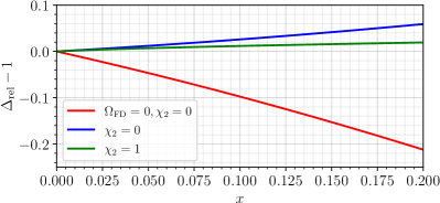
Figure 1: Relativistic effects on the resonance frequency (68) for mass ratio $q=m_{2}/m_{1}=2$. The red curve shows only the redshift effect, the blue curve neglects the companion spin, and the green curve is with “maximal” aligned spin on the companion. The effect of the black-hole spin becomes larger with increasing mass ratio, and is opposite for anti-aligned spin.

In the absence of relativistic redshift and frame-dragging effects, the resonance happens at an orbital frequency of $\omega_{f}/2$. Thus, it makes sense to normalize the relativistic resonant frequency $\omega_{\text{orb}}=\omega_{\text{orb}}^{\text{res}}$ from Eq. (67) as

$$\Delta_{\text{rel}}\equiv\frac{2\omega_{\text{orb}}^{\text{res}}}{\omega_{f}}=\frac{z}{1-\Omega_{\text{FD}}/\omega_{\text{orb}}}$$ (68)

$$=1+\nu x-\chi_{2}X_{2}^{2}x^{3/2}+\frac{9+4\nu}{6}\nu x^{2}+\operatorname{\mathcal{O}}(x^{5/2}),$$ (69)

such that $\Delta_{\text{rel}}\approx 1$ at the resonance in the absence of relativistic effects. The result for the relativistic shifts of the resonance in terms of $\Delta_{\text{rel}}$ are displayed in Fig. 1; see Sec. I.B of Ref. Steinhoff et al. (2016) for a detailed interpretation.

We see in Fig. 1 that the redshift (red curve) and frame dragging effects almost cancel out (blue curve almost at $\Delta_{\text{rel}}\approx 1$) for comparable-mass binaries. This was already noted qualitatively in Ref. Steinhoff et al. (2016), and is now quantified by Eq. (68). We note that numerical simulations of eccentric binaries, e.g. Chaurasia et al. (2018), found that the radiation emanating from the neutron-star oscillations shows only the redshift but no noticeable frame-dragging effects. This is not immediately in conflict with our observation, which considers the orbital frequency (and radiation produced by the orbital motion), but it would be desirable to investigate relativistic effects on the radiation emanating from the neutron-star oscillations analytically in future work.

The frame dragging generated by the companion spin also shifts the resonance frequency, but this effect is small for comparable-mass binaries (see the discussion above regarding the sign of this dragging). This changes with increasing mass of the companion, such that the companion spin can dominate over the orbital angular momentum. For larger mass black hole companions, however, the net effect of tidal interactions decreases and becomes more difficult to discern. To conclude, for a large part of the binary parameter space relevant for neutron stars, we can approximately neglect the relativistic effects on the resonance, $\Delta_{\text{rel}}\approx 1$. They would be important for broader applications to black hole mimickers and waveform models for third-generation detectors, which is outside the scope of this paper. For neutron star binaries, the dominant effect on the resonance is due to the spin-tidal coupling (61). We hence proceed in the next section with a Newtonian approximation and incorporate the spin-tidal interaction in the effective Love number introduced in Ref. Hinderer et al. (2016); Steinhoff et al. (2016).

VI Adapting the SEOBNRv4T model

In the preceding section, we identified the spin-tidal coupling and the corresponding shift of the tidal-resonance frequency as the most important spin effect on dynamical tides. In this section, we incorporate this spin-tidal coupling in the SEOBNRv4T model. We have implemented these modifications in the LIGO Algorithms Library LALSuite at: https://github.com/jsteinhoff/lalsuite/tree/tidal_resonance_NSspin. In this model, the dynamical $f$-mode tidal effects are included through an effective Love number, calculated in the Newtonian limit, that approximately captures the frequency-dependence of the response Hinderer et al. (2016); Steinhoff et al. (2016). The model is still relativistic since it utilizes post-Newtonian results for the tidal interaction $\sim E_{\mu\nu}E^{\mu\nu}$, currently to next-to-next-to leading order Bini et al. (2012); Henry et al. (2020a, b, c). The effective Love number is calculated from an analysis of the solution for the oscillator amplitudes $Q_{m}$ before and during the $f$-mode resonance. Below, we discuss the main modifications to this due to the Coriolis effect. A comparison to related work in Ref. Ma et al. (2020a) is given in Appendix A.

We first consider the solutions for $Q_{m}$ before the resonance. We note that the $m=0$ mode has a vanishing frequency at linear order in spin and cannot be resonantly excited. Furthermore, for $|m|=1$ the driving force (57) vanishes. Thus, the only contributions to the resonance are associated with $|m|=2$. Gathering the pre-resonance solution (where $\omega_{\text{orb}}\approx\text{const}$) for $Q_{2}=Q^{*}_{-2}$ from Eqs. (59), (57), and (60), neglecting relativistic effects from redshift $z\approx 1$ and frame dragging $\Omega_{\text{FD}}\approx 0$ (as justified in the previous section), and transforming back to the time domain leads to

$$Q_{2}=\frac{-\lambda_{0}\omega_{0}^{2}{\cal E}_{2}e^{-2i\omega_{\text{orb}}t}}{\omega_{0}^{2}-(2\omega_{\rm orb}-\Delta\omega_{0})^{2}},$$ (70)

with $\Delta\omega_{0}=-2\bar{C}_{SQ}S_{1}$, see Eq. (61). Note that although we are assuming that $\Delta\omega/\omega_{0}$ is small, we do not expand the denominator in the solution. This is important to preserve the underlying physics of the resonance shift, and is a common approach for oscillators with small perturbations to their equations of motion (e.g., for an anharmonic oscillator Landau and Lifshitz (1976)).

Near the resonance, the denominator of the solutions (70) vanishes and the dynamics require a local analysis that accounts for the evolution of $\omega_{\rm orb}$ due to gravitational radiation. This was discussed for the nonspinning case in Hinderer et al. (2016); Steinhoff et al. (2016) in terms of two-timescale expansions that exploit the hierarchy between the timescales in the system associated with the orbital motion $\sim\omega_{\rm orb}^{-1}$, the $f$-mode oscillations $\sim\omega_{0}^{-1}$, and the gravitational radiation reaction $\tilde{t}=\epsilon\phi$, where $\phi=\int\omega_{\rm orb}dt$ and $\epsilon=256\mu M^{2/3}(\omega_{f}/2)^{5/3}/5$ is a small dimensionless parameter; the temporal width of the resonance is intermediate between the orbital and radiation reaction timescales. Here, we promote these nonspinning results to the spinning case with minor but important modifications. We will obtain approximate results of the dominant effect without re-doing the entire calculations by using different physical perspectives of the Coriolis effect for the analysis away from and near the resonance, as we now discuss. The asymptotic behavior of the solution (70) near the resonance is

$$\lim_{\omega_{\rm orb}\to\frac{\omega_{0}+\Delta\omega_{0}}{2}}Q_{2}=-\frac{\lambda_{0}\bar{\cal E}e^{2i(\tilde{t}_{\rm res}/\epsilon+\hat{t}/\sqrt{\epsilon})}}{2\,\sqrt{\epsilon}\,\hat{t}\,|\bar{\Omega}^{\prime}|}+O(\hat{t}^{-3},\epsilon^{0}),$$ (71)

Here, $\hat{t}=\sqrt{\epsilon}(\phi-\phi_{\rm res})$ is a rescaled shifted phase variable and ’$\rm res$’ denotes evaluation at the resonance. The quantity $\bar{\cal E}=-{\cal E}_{2}\omega_{0}^{2}/(2\omega_{\rm orb}-\Delta\omega_{0})^{2}$ is a rescaled tidal amplitude. The function $\bar{\Omega}$ is the frequency ratio between the $f$-mode and tidal driving frequencies. Its rescaled derivative evaluated at the resonance is given by

$$\bar{\Omega}^{\prime} = \left.\frac{d}{d\tilde{t}}\left(\frac{\omega_{0}}{2\omega_{\rm orb}-\Delta\omega_{0}}\right)\right\rvert_{\rm res}$$ (72)

$$= \frac{\dot{\omega}_{\rm orb}}{\epsilon\omega_{\rm orb}}\frac{\partial}{\partial\omega_{\rm orb}}\left[\frac{\omega_{0}}{2\omega_{\rm orb}-\Delta\omega_{0}}\right]\bigg{\rvert}_{\omega_{\rm orb}=(\omega_{0}+\Delta\omega_{0})/2}$$

In the nonspinning case when $\Delta\omega_{0}=0$, this expression evaluates to be $\bar{\Omega}^{\prime}=-3/8$ using the leading order frequency evolution due to gravitational radiation reaction $\dot{\omega}_{\rm orb}=96/5\mu M^{2/3}\omega_{\rm orb}^{11/3}$. In the spinning case, however, there is an extra contribution that depends on the frequency shift and we obtain

$$\bar{\Omega}^{\prime}=-\frac{3}{8}\frac{\omega_{0}+\Delta\omega_{0}}{\omega_{0}}.$$ (73)

Next, we consider the solutions in the resonance region. In this regime, the Coriolis effect can be viewed as an effective shift in the $f$-mode frequency. This means that all the results from Steinhoff et al. (2016) carry over in a straightforward manner with the only change being a shift in $\omega_{f}$. The inner solutions are thus given by

$$Q_{2}^{\rm res} = \frac{\lambda_{0}\bar{\cal E}e^{2i\phi}}{\sqrt{\epsilon}}\bigg{[}\cos(|\tilde{\Omega}^{\prime}|\hat{t}^{2})\int_{-\infty}^{\hat{t}}\sin(|\tilde{\Omega}^{\prime}|s^{2})ds$$ (74)

$$\ \ \ \ \ \ \ -\sin(|\tilde{\Omega}^{\prime}|\hat{t}^{2})\int_{-\infty}^{\hat{t}}\cos(|\tilde{\Omega}^{\prime}|s^{2})ds\bigg{]}.\ \ \ \ \ \ \ \ \ \ \$$

The ratio of mode and tidal forcing frequencies in the near-resonance region is

$$\tilde{\Omega}=\frac{\omega_{0}+\Delta\omega_{0}}{2\omega_{\rm orb}}$$ (75)

and thus $\tilde{\Omega}^{\prime}=-3/8$ as in the nonspinning case since a modification of $\omega_{0}$ does not affect the derivatives. The asymptotic behavior of this solution away from the resonance is

$$\lim_{\omega_{\rm orb}\to\frac{\omega_{0}+\Delta\omega_{0}}{2}}Q_{2}^{\rm res}=-\frac{\lambda_{0}\bar{\cal E}e^{2i(\tilde{t}_{\rm res}/\epsilon+\hat{t}/\sqrt{\epsilon})}}{2\sqrt{\epsilon}\,\hat{t}\,|\tilde{\Omega}^{\prime}|}+O(\hat{t}^{-3},\epsilon^{0}).$$ (76)

We see from the expansions (71) and (76) that the outer (70) and inner (74) solutions match provided that we also introduce a shift in $\lambda_{0}$ in the near-resonance solutions given by

$$\lambda_{0}^{\rm near-res}=\frac{\lambda_{0}}{1+\Delta\omega_{0}/\omega_{0}}.$$ (77)

Note that as above we did not expand the denominator in $\Delta\omega_{0}$ in Eq. (77) to guarantee the matching. Finally, we can write down the composite solution for the quadrupole by combining the pre- and near-resonance solutions with the above modifications in each regime and subtracting their common singularity, as explained in Ref. Steinhoff et al. (2016). The last step is to ensure the correct limit at low frequencies $\omega_{\rm orb}/\Delta\omega_{0}\ll 1$ by including an overall factor of $(1-\Delta\omega_{0}^{2}/\omega_{0}^{2})$. We then compute the effective Love number $\Lambda_{\ell}=\lambda_{0\ell}\hat{k}^{\rm eff}_{\ell}/m_{1}^{5}$ used in the EOB code from

$$\hat{k}_{\rm eff}=-\frac{Q_{ij}E_{ij}}{\lambda_{0}E_{kl}E_{kl}}=-\frac{\sum_{m}Q_{m}E_{m}}{\lambda_{0}\sum_{m}E_{m}E_{m}}.$$ (78)

We display the results here with the convention that the sign of $\Delta\omega_{0\ell}$ depends on the spin orientation and that it is a function of the EOB coordinate $r$ through $\omega_{\rm orb}=M^{1/2}r^{-3/2}$. The dynamical tidal enhancement factor including the shifts is then given by

$$\hat{k}^{\rm eff}_{\ell} =a_{\ell}+b_{\ell}\left(1-\frac{(\Delta\omega_{0\ell})^{2}}{\omega_{0\ell}^{2}}\right)\bigg{\{}\frac{\omega_{0\ell}^{2}}{\omega_{0\ell}^{2}-(\ell\omega_{\rm orb}-\Delta\omega_{0\ell})^{2}}$$

$$+\left[\frac{\omega_{f,\ell}^{2}}{2\sqrt{\epsilon_{\ell}}\,\hat{t}\,|\tilde{\Omega}^{\prime}|\left(1+\frac{\Delta\omega_{0\ell}}{\omega_{0\ell}}\right)(\ell\omega_{\rm orb})^{2}}\right]_{\omega_{f,\ell}=\omega_{0\ell}+\Delta\omega_{0\ell}}$$

$$+\left[\frac{\omega_{f,\ell}^{2}}{\sqrt{\epsilon_{\ell}}(\ell\omega_{\rm orb})^{2}\left(1+\frac{\Delta\omega_{0\ell}}{\omega_{0\ell}}\right)}{\cal Q}_{\ell\ell}(\hat{t})\right]_{\omega_{f,\ell}=\omega_{0\ell}+\Delta\omega_{0\ell}}\bigg{\}},\ \ \$$ (79)

where

$${\cal Q}_{\ell\ell}(\hat{t}) = \cos(|\tilde{\Omega}^{\prime}|\hat{t}^{2})\int_{-\infty}^{\hat{t}}\sin(|\tilde{\Omega}^{\prime}|s^{2})ds$$ (80)

$$-\sin(|\tilde{\Omega}^{\prime}|\hat{t}^{2})\int_{-\infty}^{\hat{t}}\cos(|\tilde{\Omega}^{\prime}|s^{2})ds.$$

The quantities $\hat{t}(\omega_{f})$ and the dimensionless parameter $\epsilon_{\ell}(\omega_{f})$ are given as explicit functions of $r$ by

$$\hat{t}=\frac{8}{5\sqrt{\epsilon_{\ell}}}\left(1-\frac{r^{5/2}\omega_{f,\ell}^{5/3}}{\ell^{5/3}M^{5/6}}\right),\;\;\epsilon_{\ell}=\frac{256\mu M^{2/3}\omega_{f,\ell}^{5/3}}{5\ell^{5/3}}.$$ (81)

In Eq. (79) a body label on the quantities $\omega_{0\ell}$, $\hat{t}$, $\epsilon_{\ell}$, and ${\cal Q}_{\ell\ell}$ is implied. For each $\ell$-multipole only $|m|=\ell$ contributes in Eq. (79) because the effect of modes with $|m|\neq\ell$ has already been taken into account as adiabatic contributions. For the quadrupole and octupole multipole moments the coefficients are given by $(a_{2},a_{3})=(\frac{1}{4},\frac{3}{8})$ and $(b_{2},b_{3})=(\frac{3}{4},\frac{5}{8})$.

VII Comparisons to numerical relativity simulations

In this section, we compare the performance of the new extension of the SEOBNRv4T approximant derived in Sec. VI with numerical-relativity waveforms. We will focus on black hole – neutron star (NSBH) systems simulated with the SpEC code SPE (2018); Duez et al. (2008); Foucart et al. (2013) and on binary neutron star (NSNS) simulations with the BAM code Bruegmann et al. (2008); Thierfelder et al. (2011); Dietrich et al. (2015).

In addition to the quantitative comparison that we will show in the next subsections, numerical-relativity simulations provide also a qualitative indication for the importance of non-equilibrium tides. Figure 2 shows a NSBH system with mass ratio $q=m_{2}/m_{1}=1$ and an anti-aligned neutron star spin, which enhances the excitation of non-equilibrium tides as discussed in Sec. V and can be seen from Eq. (79) with a negative $\Delta\omega_{0\ell}$. While it is difficult to directly quantify these dynamical tides in a gauge-independent manner, the visual difference in Fig. 2 between the spinning and non-spinning matter distributions of the neutron star – which have no invariant meaning – provide an illustration of measurable differences in waveforms that we will analyze below.

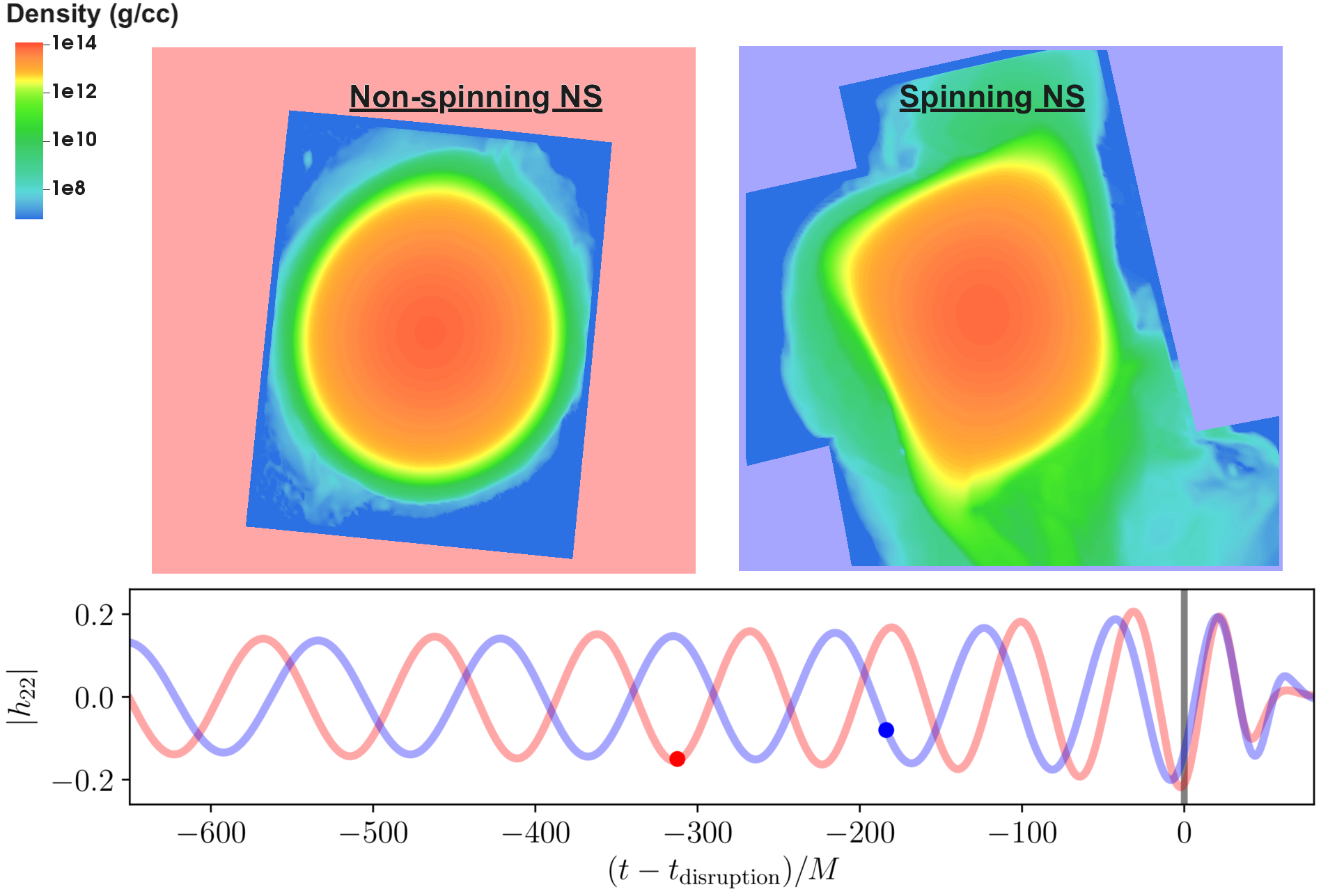
Figure 2: Matter density in the late inspiral for the non-spinning $q=1$ NSBH simulation (top left), and for the simulation with a spinning neutron star (top right), as well as the corresponding GW signal. We show the density in the equatorial plane at a time when the binary separation is $\sim 35\,{\rm km}$; cf. markers in the bottom panel. The differences in the amount of distortion in the matter distributions (larger for the spinning NS) and onset of tidal disruption (earlier for the spinning NS), while being purely gauge-dependent, can be considered as a visualization of the enhancement of non-equilibrium tides. The waveforms are aligned at the tidal disruption as determined from the peak GW amplitude.

VII.1 Comparison to NSBH SXS waveforms

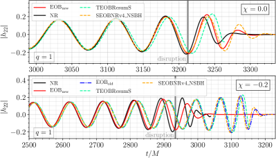
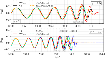
Figure 3: Comparisons of various models to the NR waveforms for NSBH considered in this work (top – equal mass and bottom – mass ratio $q=2$). The TEOBResumS waveforms are tapered to zero after the NSNS merger frequency, and the SEOBNR waveforms are tapered either at the NSNS merger or the $f$-mode resonance, whichever occurs first. Remarkably, the $f$-mode resonance in our new model including the spin shifts matches quite well with the tidal disruption frequency in the NR data, while the models that do not include the spin shifts predict a merger at a later time.

For an initial comparison to numerical-relativity simulations and a validation of our new model, we consider two NSBH setups presented in Ref. Foucart et al. (2019) and simulated with the SpEC code SPE (2018); Duez et al. (2008); Foucart et al. (2013). The two configurations represent an equal-mass $q=1$ and an unequal-mass $q=2$ setup employing a single polytropic equation of state $P=\kappa\rho^{2}$, with $\kappa$ chosen so that $m_{1}/R_{1}=0.144$ (e.g.. $R_{1}=13.8\,{\rm km}$ if $m_{1}=1.35M_{\odot}$). Each mass ratio is simulated twice: with a non-spinning neutron star and with an anti-aligned dimensionless spin $\chi_{1}=-0.2$ on the neutron star. In both cases the black hole remains non-spinning. The neutron star spins and mass ratios were chosen as examples of a large expected impact of non-equilibrium tides. The numerical relativity data are publicly available in the SXS catalog Boyle et al. (2019), where we use the simulations SXS:BHNS:0004 and SXS:BHNS:0005 for the $q=1$ and SXS:BHNS:0002 and SXS:BHNS:0007 for the $q=2$, nonspinning and spinning cases, respectively.

The evolutions start $10-13$ orbits before merger and use eccentricity-reduced ($e<0.002$), constraint satisfying initial conditions Foucart et al. (2008); Pfeiffer et al. (2007). Each case is simulated at three resolutions, and a detailed discussion of the estimated numerical error in these simulations can be found in Ref. Foucart et al. (2019). The same error estimates are used in this work. We typically find phase errors of less than $0.1\,{\rm rad}$ for most of the inspiral and rising to $(0.1-0.2)\,{\rm rad}$ at merger for the $q=1$ cases and to $(0.5-1.0)\,{\rm rad}$ for $q=2$.

We show in Fig. 3 the real part of the GW for the dominant (2,2)-mode for the two different mass ratios and different spin. The parameters that we use in the EOB models were not obtained from quasi-universal relations [except for the fit in Eq. (62)] and read

$$\frac{\lambda_{0}}{m_{1}^{5}} =799.3, m_{1}\omega_{0} =0.06746,$$ (82)

$$\frac{\Delta\omega_{0}}{\omega_{0}} =-0.325, \frac{\lambda_{03}}{m_{1}^{7}} =2246,$$ (83)

$$m_{1}\omega_{03} =0.08805, \frac{\Delta\omega_{03}}{\omega_{03}} =-0.4,$$ (84)

$$C_{ES^{2}} =7.14, \frac{I}{m_{1}^{3}} =15.5,$$ (85)

recalling that these are the (quadrupolar, $\ell=2$) Love number $\lambda_{0}$, nonspinning $f$-mode frequency $\omega_{0}$, the mode shift $\Delta\omega_{0}$ due to spin, the corresponding octupolar ($\ell=3$) values $\lambda_{03}$, $\omega_{03}$, $\Delta\omega_{03}$, the dimensionless spin-induced quadrupole-moment constant $C_{ES^{2}}$ (normalized to 1 for black holes), and the moment of inertia $I$. We see from these plots that for the nonspinning cases, existing waveform models predict the length of the waveforms and decrease of the GW amplitude due to the tidal disruption of the neutron star to a good approximation. However, for systems with anti-aligned spins, all existing models, including those specialized for NSBH systems predict longer waveforms, while the new modification with spin effects (red curve) continues to yield a good prediction for the length of the signal. This is because in our new model, as also in the nonspinning SEOBNRv4T model, the GW signal is tapered to zero once the system reaches the $f$-mode resonance, if it occurs before the NSNS merger frequency. The fact that for the new SEOBNRv4T model the tapering occurs at the $f$-mode resonance for these cases can be seen by comparing to the TEOBResumS results, which are always tapered at the NSNS merger frequency. These findings highlight an interesting point, namely that there seems to be a direct relation between the $f$-mode resonance and the tidal disruption frequency.

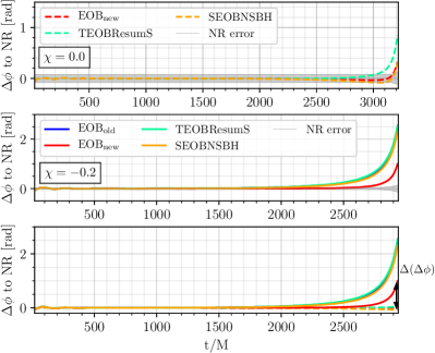
Figure 4: Phase differences in the NSBH case for different approximants and the numerical-relativity simulations. We consider the difference of the phase difference in the spinning minus the nonspinning case for the $q=1$ NSBH simulation described in the main text to quantify systematic dependencies on the spin. The top panel shows phase difference between the numerical-relativity simulation (and its uncertainty shown as a gray band) with the TEOBResumS, SEOBNRv4T, and SEOBNSBH models. The middle panel shows a similar comparison for an anti-aligned neutron star spin, where we also add the new SEOBNRv4T model described in this article. In the bottom panel, we highlight again the phase difference between the approximants and the simulation results in the spinning and non-spinning case. The difference between the phase difference, i.e., $\Delta(\Delta\phi)$, is for the newly implemented model smallest.

Focusing on the $q=1$ setup, we next show the phase difference between the old (without the Coriolis effect) and the new SEOBNRv4T model, as well as results for TEOBResumS Nagar et al. (2018) and SEOBNSBH Matas et al. (2020) in Fig. 4. For the non-spinning case (top panel) all models describe the GW phase accurately up to about one orbit before merger and stay within the estimated uncertainty of the numerical-relativity simulation (shown as the gray shaded region) Foucart et al. (2019). Considering the middle panel of Fig. 4, the anti-aligned spin of the neutron star enhances the dynamical tidal effects. We find that for this setup, the discrepancy in phasing between the new SEOBNRv4T model and the numerical relativity results is significantly less than for the other approximants. Therefore, we find a significantly better performance if non-equilibrium tidal effects are included. Although the new version of SEOBNRv4T is outside the estimated numerical uncertainty band close to the tidal disruption, other approximants show a noticeable dephasing even a few orbits before the disruption of the star, and it is this earlier-time regime where we expect to have more analytical control over the physics of the model.

An even more important diagnostic of the robustness of our model, beyond a reduced phase difference in a few example cases, is that the phase differences to the numerical-relativity simulations are consistent between the spinning and non-spinning setups. To test the performance of our model with regards to this criterion we introduce the quantity $\Delta(\Delta)\phi$, which measures the phase difference for the case with spin minus the phase difference in the corresponding nonspinning case. A small $\Delta(\Delta)\phi$ indicates that the physics of the dynamical tidal effects and impact of the Coriolis effect are well-captured by the model, up to other physical effects with a different origin that are common among all cases. The definition of $\Delta(\Delta)\phi$ is illustrated in the bottom panel of Fig. 4 showing the phase difference between the EOB model and the SpEC data in the spinning case minus the phase difference for the non-spinning setup, i.e., the smaller the difference the better the consistency between the non-spinning and spinning data.

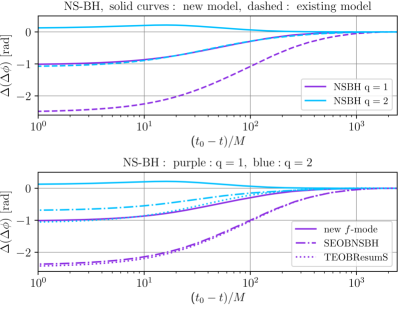
Figure 5: Phase differences compared to the phase differences in the nonspinning case for the NSBH configurations. Top panel: Solid curves are the new model developed in this paper, dashed curves are the existing SEOBNRv4T model, which does not account for spin effects on the mode resonances and exhibits a wider spread in phase differences between spinning and non-spinning configurations. Bottom panel: Comparison with other waveform models which do not incorporate the spin-induced shift of the $f$-mode. We see that the new model has a consistently smaller spread. In each case, $t_{0}$ is the time at which the first merger occurs (i.e. for aligned spins it is the nonspinning merger, and otherwise the merger of the anti-aligned configuration).

For a more quantitative presentation, we present $\Delta(\Delta\phi)$ for the new and old SEOBNRv4T model in the top panel of Fig. 5 for the $q=1$ and $q=2$ setup. This clearly shows that for both configurations the new model outperforms the previous implementation. Similarly, the bottom panel shows also the new model in comparison to other NSBH approximants, where the disagreement between phase difference for spinning and non-spinning with respect to the corresponding numerical-relativity simulations is larger than for the model developed in this paper.

VII.2 NSNS BAM waveforms

Table 1: NSNS-BAM configurations. The first column defines the name of the configuration with the notation: EOS${}_{m^{A}}^{\chi^{A}}$. The subsequent columns describe: the EOS Read et al. (2009), the NS’ individual masses $m_{A,B}$, the stars’ dimensionless spins $\chi_{A,B}$, the Love number $\lambda_{0}$, the nonspinning $f$-mode frequency $\omega_{0}$, the mode shift $\Delta\omega_{0}$ due to spin, the corresponding octupolar ($\ell=3$) values $\lambda_{03}$, $\omega_{03}$, $\Delta\omega_{03}$, the dimensionless spin-induced quadrupole-moment constant $C_{ES^{2}}$ (normalized to 1 for black holes), and the moment of inertia $I$. The values here were not obtained from quasi-universal relations, except for the fit in Eq. (62).

Name	EOS	$m_{1,2}/M_{\odot}$	$\chi_{1,2}$	$\lambda_{0}/m_{1}^{5}$	$m_{1}\omega_{0}$	$\Delta\omega_{0}/\omega_{0}$	$\lambda_{03}/m_{1}^{7}$	$m_{1}\omega_{03}$	$\Delta\omega_{03}/\omega_{03}$	$C_{ES^{2}}$	$I/m_{1}^{3}$
MS1b${}_{1.35}^{-0.10}$	MS1b	1.3504	$-0.099$	1528	0.05836	$-0.137$	4488	0.07973	$-0.162$	8.74	18.05
MS1b${}_{1.35}^{0.00}$	MS1b	1.3500	$+0.000$	1528	0.05836	$+0.000$	4488	0.07973	$+0.000$	—	—
MS1b${}_{1.35}^{0.10}$	MS1b	1.3504	$+0.099$	1528	0.05836	$+0.145$	4488	0.07973	$+0.164$	8.74	18.05
MS1b${}_{1.35}^{0.15}$	MS1b	1.3509	$+0.149$	1525	0.05837	$+0.210$	4474	0.07977	$+0.238$	8.54	18.17
H4${}_{1.37}^{0.00}$	H4	1.3717	$+0.000$	1003	0.06435	$+0.000$	2605	0.08702	$+0.000$	—	—
H4${}_{1.37}^{0.14}$	H4	1.3726	$+0.141$	1003	0.06435	$+0.202$	2605	0.08702	$+0.232$	7.32	16.11
SLy${}_{1.35}^{0.00}$	SLy	1.3500	$+0.000$	389.6	0.07934	$+0.000$	705.2	0.1067	$+0.000$	—	—
SLy${}_{1.35}^{0.05}$	SLy	1.3502	$+0.052$	389.6	0.07934	$+0.084$	705.2	0.1067	$+0.096$	6.18	12.34
SLy${}_{1.35}^{0.11}$	SLy	1.3506	$+0.106$	388.8	0.07936	$+0.164$	703.4	0.1068	$+0.189$	5.59	12.41

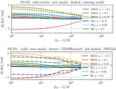
Figure 6: Phase differences compared to the phase differences in the nonspinning case for the NSNS configurations. Top panel: Solid curves are the new model developed in this paper, dashed curves are the existing SEOBNRv4T model, which does not account for spin effects on the mode resonances and exhibits a wider spread in phase differences between spinning and non-spinning configurations. Bottom panel: Comparison with other waveform models which do not incorporate the spin-induced shift of the $f$-mode. We see that the new model has a consistently smaller spread. In each case, $t_{0}$ is the time at which the first merger occurs (i.e. for aligned spins it is the nonspinning merger, and otherwise the merger of the anti-aligned configuration).

We continue our tests of the new model by comparing against numerical-relativity waveforms of NSNS systems computed with the BAM code Dietrich et al. (2017, 2018a, 2018b, 2019a), which include cases with both aligned and anti-aligned spins. In total, we consider three different equations of state: SLy, H4, MS1b. For all these equations of state, we consider one non-spinning configuration and one to three spinning setups; cf. Tab. 1 for further details and for the parameters used in the EOB models. The waveforms from Ref. Dietrich et al. (2018a) show a clean second-order convergence, which allows using Richardson extrapolation to obtain a better guess for the true waveform, as discussed in Ref. Bernuzzi and Dietrich (2016). We use the Richardson-extrapolated data from Ref. Dietrich et al. (2018a) for our comparisons.

For all the cases, we follow a similar procedure as for the NSBH setups by focusing on the difference of the phase difference between the spinning EOB and the numerical-relativity waveforms with respect to their non-spinning counterparts. This way, we explicitly test the imprint of spin on the dynamical tides. Our results are summarized in Fig. 6, where in the top panel the dashed lines refer to the old SEOBNRv4T model without the spin effects on the dynamical tides, and the solid lines show results for our new model. We find that for these cases, the new model shows a smaller phase difference between the numerical-relativity and the EOB data as the old model. We emphasize that this does not necessarily mean that the total phase difference with respect to the numerical-relativity data decreased in all cases, but rather that the phase difference for the non-spinning and spinning configurations becomes almost identical, indicating that the dependence on parameters is captured well.

The bottom panel of Fig. 6 compares the consistency of various GW models Nagar et al. (2018); Dietrich et al. (2019a) between the spinning and the non-spinning configurations for the NSNS binaries. We find that for all the setups the new SEOBNRv4T implementation has the smallest $\Delta(\Delta\phi)$, which means that the phase difference between the EOB model and the NR simulation is similar for the spinning and non-spinning cases. These results indicate that (i) the inclusion of spin-effects is consistent and (ii) further improvements of the non-spinning sector will likely also improve the agreement between EOB and numerical-relativity predictions for spinning configurations.

VIII Conclusions

In this paper, we developed a ready-to-use waveform model that approximately captures the effects of spin on the $f$-mode dynamical tidal response of a neutron star. This model is based on the leading order terms in a relativistic effective action describing a spinning neutron star in a binary system, which we derived.

We found that within our approximation, a nonvanishing spin gives rise to a Coriolis interaction term in the action. We determined the coupling coefficient for this term from the spin-induced shift of the $f$-mode frequencies in slowly rotating relativistic neutron stars. A quasi-universal relation for this coupling coefficient was found as well, which is important for reducing the number of parameters to be inferred from GW observations. Further, using explicit post-Newtonian results we also analyzed relativistic effects (redshift and frame dragging) on the dynamical tidal response and found that they are subdominant compared to the spin effects.

We then developed a simple model that captures the main Coriolis effects on dynamical tides and incorporated it into a state-of-the-art EOB model. To test this new model, we performed comparisons to results from numerical relativity simulations of binary neutron star and neutron-star–black-hole binaries. The new model showed improved behavior over the parameter space compared to existing models that neglect the Coriolis effect. Moreover, we found that it predicted the tidal disruption frequency in mixed binaries significantly better than models without this spin-tidal effect. Our model is implemented in the LIGO Algorithms library.

This work also identified important directions for future work. Moreover, the results from this paper provide a useful foundation for including these spin-tidal effects also in other waveform models. Improving the physics content of models is important for accurate measurements and robustness over a wider range in parameter space. We have also derived the relativistic effects on the response which can be included in future models, when we will also work out the effective Love number based on the spin-dependent response, allow for misaligned spins and other effects of the companion’s spin, and also include other relativistic effects in a binary system.

Appendix A Connection to Ma, Yu, and Chen Ma et al. (2020a)

Here, we briefly outline similarities and differences with the work of Ma, Yu and Chen (hereafter MYC20) in Ref. Ma et al. (2020a), which considered the effect of spin on the $f$-mode in a Newtonian context. The effect of spins on the tidal response in Ref. Ma et al. (2020a) is interconnected with the orbital dynamics obtained from numerical integrations of the equations of motion for the coupled system of dynamical quadrupoles, orbital variables, and gravitational radiation reaction. For ease of comparing to our results here, we apply the same procedure as for obtaining the effective Love number $\hat{k}_{2}^{\rm eff}$ oulined in Sec: VI to write the formulae in MYC20 explicitly as functions of the orbital separation $r$. The choice of this variable is motivated by the fact that the canonical coordinate $r$ plays a key role for the EOB dynamics, which are the basis of EOB waveforms. The formulae in Ref. Ma et al. (2020a) are similar to our results, with slight differences in the definitions of variables such as $\hat{t}$ leading to small differences in the response near the resonance, as illustrated in Fig. 7. For instance, in our work, $\hat{t}$ is based on the phase and the parameter $\epsilon$, while in MYC20 $\hat{t}^{Y}$ is based on coordinate time and $\dot{\omega}$ at the resonance time and given explicitly by

$$\hat{t}^{Y}=\frac{\sqrt{15}}{16\,2^{2/3}M^{1/3}\sqrt{\mu}\;w}-\frac{\sqrt{15}r^{4}\;w}{128\,2^{1/3}M^{5/3}\sqrt{\mu}}$$ (86)

where

$$w=\sqrt{-\omega_{-}\omega_{+}+\Omega^{2}}-\Omega.$$ (87)

Here, $|\omega_{\pm}|$ are the frequencies of the two branches of $m$-modes whose frequencies coincide for $\Omega=0$.

MYC20 compute the $f$-mode frequencies for Newtonian Maclaurin spheroids. In the nonspinning case, this yields frequencies that are $\sim 320$Hz smaller than the relativistic values. MYC20 account for this by rescaling the density so as to match the relativistic frequencies. In this paper, we have used the fully relativistic results for the frequencies and their shifts, albeit only within the linear approximation for small $\Omega$. The variables of MYC20 are approximately related to these shifts by $|\omega_{\pm}|\approx\omega_{0}\mp\Delta\omega$. These different approximations and prescriptions also affect the orbital frequency at resonance. For instance, for the case of $\Omega=2\pi 550$Hz considered in MYC20, which is already outside of the linear regime, the resonance occurs at $\sim 300$Hz for MTY20 but not until $\sim 350$Hz for the parameters used here. The resulting predictions for the effective Love number are illustrated in Fig. 8.

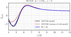
Figure 7: Analytical approximations for a nonspinning equal-mass binary with one extended body. Here, MYC20 is from Eq. (54) with the higher-order matching from Eq. (55) in Ref. Ma et al. (2020a).

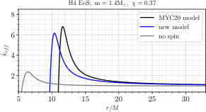
Figure 8: Comparison between the model developed in this paper with $\{\Delta\omega_{0},\Delta\lambda\}$ and MYC20 for a spin frequency $\Omega=2\pi\times 550$Hz. For reference, the grey curve indicates the nonspinning result.

References

- Lattimer and Prakash (2016) J. M. Lattimer and M. Prakash, “The Equation of State of Hot, Dense Matter and Neutron Stars,” Phys. Rept. 621, 127–164 (2016), arXiv:1512.07820 [astro-ph.SR] .
- Rezzolla et al. (2018a) L. Rezzolla, P. Pizzochero, D. I. Jones, N. Rea, and I. Vidaña, “The Physics and Astrophysics of Neutron Stars,” Astrophys. Space Sci. Libr. 457, pp.– (2018a).
- Abbott et al. (2017a) B. P. Abbott et al. (LIGO Scientific, Virgo), “Search for Post-merger Gravitational Waves from the Remnant of the Binary Neutron Star Merger GW170817,” Astrophys. J. Lett. 851, L16 (2017a), arXiv:1710.09320 [astro-ph.HE] .
- Abbott et al. (2019) B. P. Abbott et al. (LIGO Scientific, Virgo), “Properties of the binary neutron star merger GW170817,” Phys. Rev. X9, 011001 (2019), arXiv:1805.11579 [gr-qc] .
- Abbott et al. (2017b) B. P. Abbott et al. (LIGO Scientific, Virgo), “GW170817: Observation of Gravitational Waves from a Binary Neutron Star Inspiral,” Phys. Rev. Lett. 119, 161101 (2017b), arXiv:1710.05832 [gr-qc] .
- Bauswein et al. (2017) A. Bauswein, O. Just, H.-T. Janka, and N. Stergioulas, “Neutron-star radius constraints from GW170817 and future detections,” Astrophys. J. Lett. 850, L34 (2017), arXiv:1710.06843 [astro-ph.HE] .
- Annala et al. (2018) E. Annala, T. Gorda, A. Kurkela, and A. Vuorinen, “Gravitational-wave constraints on the neutron-star-matter Equation of State,” Phys. Rev. Lett. 120, 172703 (2018), arXiv:1711.02644 [astro-ph.HE] .
- Most et al. (2018) E. R. Most, L. R. Weih, L. Rezzolla, and J. Schaffner-Bielich, “New constraints on radii and tidal deformabilities of neutron stars from GW170817,” Phys. Rev. Lett. 120, 261103 (2018), arXiv:1803.00549 [gr-qc] .
- Ruiz et al. (2018) M. Ruiz, S. L. Shapiro, and A. Tsokaros, “GW170817, General Relativistic Magnetohydrodynamic Simulations, and the Neutron Star Maximum Mass,” Phys. Rev. D97, 021501 (2018), arXiv:1711.00473 [astro-ph.HE] .
- Margalit and Metzger (2017) B. Margalit and B. D. Metzger, “Constraining the Maximum Mass of Neutron Stars From Multi-Messenger Observations of GW170817,” Astrophys. J. Lett. 850, L19 (2017), arXiv:1710.05938 [astro-ph.HE] .
- Rezzolla et al. (2018b) L. Rezzolla, E. R. Most, and L. R. Weih, “Using gravitational-wave observations and quasi-universal relations to constrain the maximum mass of neutron stars,” Astrophys. J. Lett. 852, L25 (2018b), arXiv:1711.00314 [astro-ph.HE] .
- Shibata et al. (2017) M. Shibata, S. Fujibayashi, K. Hotokezaka, K. Kiuchi, K. Kyutoku, Y. Sekiguchi, and M. Tanaka, “Modeling GW170817 based on numerical relativity and its implications,” Phys. Rev. D96, 123012 (2017), arXiv:1710.07579 [astro-ph.HE] .
- Abbott et al. (2018) B. P. Abbott et al. (LIGO Scientific, Virgo), “GW170817: Measurements of neutron star radii and equation of state,” Phys. Rev. Lett. 121, 161101 (2018), arXiv:1805.11581 [gr-qc] .
- De et al. (2018) S. De, D. Finstad, J. M. Lattimer, D. A. Brown, E. Berger, and C. M. Biwer, “Tidal Deformabilities and Radii of Neutron Stars from the Observation of GW170817,” Phys. Rev. Lett. 121, 091102 (2018), [Erratum: Phys. Rev. Lett.121,no.25,259902(2018)], arXiv:1804.08583 [astro-ph.HE] .
- Radice et al. (2018) D. Radice, A. Perego, F. Zappa, and S. Bernuzzi, “GW170817: Joint Constraint on the Neutron Star Equation of State from Multimessenger Observations,” Astrophys. J. Lett. 852, L29 (2018), arXiv:1711.03647 [astro-ph.HE] .
- Coughlin et al. (2018) M. W. Coughlin et al., “Constraints on the neutron star equation of state from AT2017gfo using radiative transfer simulations,” Mon. Not. Roy. Astron. Soc. 480, 3871–3878 (2018), arXiv:1805.09371 [astro-ph.HE] .
- Coughlin et al. (2019) M. W. Coughlin, T. Dietrich, B. Margalit, and B. D. Metzger, “Multimessenger Bayesian parameter inference of a binary neutron star merger,” Mon. Not. Roy. Astron. Soc. 489, L91–L96 (2019), arXiv:1812.04803 [astro-ph.HE] .
- Dai et al. (2018) L. Dai, T. Venumadhav, and B. Zackay, “Parameter Estimation for GW170817 using Relative Binning,” (2018), arXiv:1806.08793 [gr-qc] .
- Radice and Dai (2019) D. Radice and L. Dai, “Multimessenger Parameter Estimation of GW170817,” Eur. Phys. J. A55, 50 (2019), arXiv:1810.12917 [astro-ph.HE] .
- Lucca and Sagunski (2020) M. Lucca and L. Sagunski, “The lifetime of binary neutron star merger remnants,” JHEAp 27, 33–37 (2020), arXiv:1909.08631 [astro-ph.HE] .
- Capano et al. (2020) C. D. Capano, I. Tews, S. M. Brown, B. Margalit, S. De, S. Kumar, D. A. Brown, B. Krishnan, and S. Reddy, “Stringent constraints on neutron-star radii from multimessenger observations and nuclear theory,” Nature Astron. 4, 625–632 (2020), arXiv:1908.10352 [astro-ph.HE] .
- Dietrich et al. (2020a) T. Dietrich, M. W. Coughlin, P. T. H. Pang, M. Bulla, J. Heinzel, L. Issa, I. Tews, and S. Antier, “Multimessenger constraints on the neutron-star equation of state and the Hubble constant,” Science 370, 1450–1453 (2020a), arXiv:2002.11355 [astro-ph.HE] .
- Raaijmakers et al. (2020) G. Raaijmakers et al., “Constraining the dense matter equation of state with joint analysis of NICER and LIGO/Virgo measurements,” Astrophys. J. Lett. 893, L21 (2020), arXiv:1912.11031 [astro-ph.HE] .
- Cutler and Flanagan (1994) C. Cutler and E. E. Flanagan, “Gravitational waves from merging compact binaries: How accurately can one extract the binary’s parameters from the inspiral wave form?” Phys. Rev. D49, 2658–2697 (1994), arXiv:gr-qc/9402014 [gr-qc] .
- Veitch et al. (2015) J. Veitch et al., “Parameter estimation for compact binaries with ground-based gravitational-wave observations using the LALInference software library,” Phys. Rev. D91, 042003 (2015), arXiv:1409.7215 [gr-qc] .
- Abbott et al. (2020) B. P. Abbott et al. (LIGO Scientific, Virgo), “A guide to LIGO–Virgo detector noise and extraction of transient gravitational-wave signals,” Class. Quant. Grav. 37, 055002 (2020), arXiv:1908.11170 [gr-qc] .
- Carter (1971) B. Carter, “Axisymmetric Black Hole Has Only Two Degrees of Freedom,” Phys. Rev. Lett. 26, 331–333 (1971).
- Hawking (1972) S. W. Hawking, “Black holes in general relativity,” Commun. Math. Phys. 25, 152–166 (1972).
- Gürlebeck (2015) N. Gürlebeck, “No-hair theorem for Black Holes in Astrophysical Environments,” Phys. Rev. Lett. 114, 151102 (2015), arXiv:1503.03240 [gr-qc] .
- Bildsten and Cutler (1992) L. Bildsten and C. Cutler, “Tidal interactions of inspiraling compact binaries,” Astrophys. J. 400, 175–180 (1992).
- Reisenegger and Goldreich (1994) A. Reisenegger and P. Goldreich, “Excitation of Neutron Star Normal Modes during Binary Inspiral,” ApJ 426, 688 (1994).
- Lai et al. (1993) D. Lai, F. A. Rasio, and S. L. Shapiro, “Ellipsoidal figures of equilibrium - Compressible models,” Astrophys. J. Suppl. 88, 205–252 (1993).
- Lai (1994) D. Lai, “Resonant oscillations and tidal heating in coalescing binary neutron stars,” Mon. Not. Roy. Astron. Soc. 270, 611 (1994), arXiv:astro-ph/9404062 [astro-ph] .
- Zahn (1977) J. P. Zahn, “Reprint of 1977A&A….57..383Z. Tidal friction in close binary stars.” A&A 500, 121–132 (1977).
- Willems et al. (2003) B. Willems, T. Van Hoolst, and P. Smeyers, “Nonadiabatic resonant dynamic tides and orbital evolution in close binaries,” Astron. Astrophys. 397, 973–986 (2003), arXiv:astro-ph/0211198 [astro-ph] .
- Zahn (1970) J. P. Zahn, “Forced Oscillations in Close Binaries. The Adiabatic Approximation,” A&A 4, 452 (1970).
- Kopal (1978) Z. Kopal, Dynamics of close binary systems (1978).
- Kochanek (1992) C. S. Kochanek, “Coalescing binary neutron stars,” Astrophys. J. 398, 234 (1992).
- Hansen (2006) D. Hansen, “Dynamical evolution and leading order gravitational wave emission of Riemann-S binaries,” Gen. Rel. Grav. 38, 1173–1208 (2006), arXiv:gr-qc/0511033 [gr-qc] .
- Mora and Will (2004) T. Mora and C. M. Will, “A PostNewtonian diagnostic of quasiequilibrium binary configurations of compact objects,” Phys. Rev. D69, 104021 (2004), [Erratum: Phys. Rev.D71,129901(2005)], arXiv:gr-qc/0312082 [gr-qc] .
- Kokkotas and Schaefer (1995) K. D. Kokkotas and G. Schaefer, “Tidal and tidal resonant effects in coalescing binaries,” Mon. Not. Roy. Astron. Soc. 275, 301 (1995), arXiv:gr-qc/9502034 [gr-qc] .
- Flanagan and Hinderer (2008) E. E. Flanagan and T. Hinderer, “Constraining neutron star tidal Love numbers with gravitational wave detectors,” Phys. Rev. D77, 021502 (2008), arXiv:0709.1915 [astro-ph] .
- Ferrari et al. (2012) V. Ferrari, L. Gualtieri, and A. Maselli, “Tidal interaction in compact binaries: a post-Newtonian affine framework,” Phys. Rev. D85, 044045 (2012), arXiv:1111.6607 [gr-qc] .
- Damour et al. (1992) T. Damour, M. Soffel, and C.-m. Xu, “General relativistic celestial mechanics. 2. Translational equations of motion,” Phys. Rev. D45, 1017–1044 (1992).
- Shibata (1994) M. Shibata, “Effects of tidal resonances in coalescing compact binary systems,” Prog. Theor. Phys. 91, 871–884 (1994).
- Rathore et al. (2003) Y. Rathore, A. E. Broderick, and R. Blandford, “A variational formalism for tidal excitation: non-rotating, homentropic stars,” Mon. Not. Roy. Astron. Soc. 339, 25 (2003), arXiv:astro-ph/0209003 [astro-ph] .
- Vines and Flanagan (2013) J. E. Vines and E. E. Flanagan, “Post-1-Newtonian quadrupole tidal interactions in binary systems,” Phys. Rev. D88, 024046 (2013), arXiv:1009.4919 [gr-qc] .
- Vines et al. (2011) J. Vines, E. E. Flanagan, and T. Hinderer, “Post-1-Newtonian tidal effects in the gravitational waveform from binary inspirals,” Phys. Rev. D83, 084051 (2011), arXiv:1101.1673 [gr-qc] .
- Chakrabarti et al. (2013a) S. Chakrabarti, T. Delsate, and J. Steinhoff, “Effective action and linear response of compact objects in Newtonian gravity,” Phys. Rev. D88, 084038 (2013a), arXiv:1306.5820 [gr-qc] .
- Andersson and Ho (2018) N. Andersson and W. C. G. Ho, “Using gravitational-wave data to constrain dynamical tides in neutron star binaries,” Phys. Rev. D97, 023016 (2018), arXiv:1710.05950 [astro-ph.HE] .
- Yu and Weinberg (2017) H. Yu and N. N. Weinberg, “Resonant tidal excitation of superfluid neutron stars in coalescing binaries,” Mon. Not. Roy. Astron. Soc. 464, 2622–2637 (2017), arXiv:1610.00745 [astro-ph.HE] .
- Tsang (2013) D. Tsang, “Shattering Flares During Close Encounters of Neutron Stars,” Astrophys. J. 777, 103 (2013), arXiv:1307.3554 [astro-ph.HE] .
- Tsang et al. (2012) D. Tsang, J. S. Read, T. Hinderer, A. L. Piro, and R. Bondarescu, “Resonant Shattering of Neutron Star Crusts,” Phys. Rev. Lett. 108, 011102 (2012), arXiv:1110.0467 [astro-ph.HE] .
- Pnigouras (2019) P. Pnigouras, “Gravitational-wave-driven tidal secular instability in neutron star binaries,” Phys. Rev. D100, 063016 (2019), arXiv:1909.04490 [astro-ph.HE] .
- Pratten et al. (2020a) G. Pratten, P. Schmidt, and T. Hinderer, “Gravitational-Wave Asteroseismology with Fundamental Modes from Compact Binary Inspirals,” Nature Commun. 11, 2553 (2020a), arXiv:1905.00817 [gr-qc] .
- Schmidt and Hinderer (2019) P. Schmidt and T. Hinderer, “Frequency domain model of -mode dynamic tides in gravitational waveforms from compact binary inspirals,” Phys. Rev. D100, 021501 (2019), arXiv:1905.00818 [gr-qc] .
- Suvorov and Kokkotas (2020) A. G. Suvorov and K. D. Kokkotas, “Precursor flares of short gamma-ray bursts from crust yielding due to tidal resonances in coalescing binaries of rotating, magnetized neutron stars,” Phys. Rev. D101, 083002 (2020), arXiv:2003.05673 [astro-ph.HE] .
- Andersson and Pnigouras (2020) N. Andersson and P. Pnigouras, “Exploring the effective tidal deformability of neutron stars,” Phys. Rev. D101, 083001 (2020), arXiv:1906.08982 [astro-ph.HE] .
- Pan et al. (2020) Z. Pan, Z. Lyu, B. Bonga, N. Ortiz, and H. Yang, “Probing Crust Meltdown in Inspiraling Binary Neutron Stars,” Phys. Rev. Lett. 125, 201102 (2020), arXiv:2003.03330 [astro-ph.HE] .
- Ng et al. (2020) H. H.-Y. Ng, P. C.-K. Cheong, L.-M. Lin, and T. G. F. Li, “Gravitational-wave asteroseismology with f-modes from neutron star binaries at the merger phase,” (2020), arXiv:2012.08263 [astro-ph.HE] .
- Pons et al. (2002) J. A. Pons, E. Berti, L. Gualtieri, G. Miniutti, and V. Ferrari, “Gravitational signals emitted by a point mass orbiting a neutron star: Effects of stellar structure,” Phys. Rev. D65, 104021 (2002), arXiv:gr-qc/0111104 [gr-qc] .
- Gualtieri et al. (2001) L. Gualtieri, E. Berti, J. A. Pons, G. Miniutti, and V. Ferrari, “Gravitational signals emitted by a point mass orbiting a neutron star: A Perturbative approach,” Phys. Rev. D64, 104007 (2001), arXiv:gr-qc/0107046 [gr-qc] .
- Krishnendu et al. (2017) N. V. Krishnendu, K. G. Arun, and C. K. Mishra, “Testing the binary black hole nature of a compact binary coalescence,” Phys. Rev. Lett. 119, 091101 (2017), arXiv:1701.06318 [gr-qc] .
- Bohé et al. (2015) A. Bohé, G. Faye, S. Marsat, and E. K. Porter, “Quadratic-in-spin effects in the orbital dynamics and gravitational-wave energy flux of compact binaries at the 3PN order,” Class. Quant. Grav. 32, 195010 (2015), arXiv:1501.01529 [gr-qc] .
- Marsat (2015) S. Marsat, “Cubic order spin effects in the dynamics and gravitational wave energy flux of compact object binaries,” Class. Quant. Grav. 32, 085008 (2015), arXiv:1411.4118 [gr-qc] .
- Levi and Steinhoff (2015a) M. Levi and J. Steinhoff, “Spinning gravitating objects in the effective field theory in the post-Newtonian scheme,” JHEP 09, 219 (2015a), arXiv:1501.04956 [gr-qc] .
- Porto et al. (2012) R. A. Porto, A. Ross, and I. Z. Rothstein, “Spin induced multipole moments for the gravitational wave amplitude from binary inspirals to 2.5 Post-Newtonian order,” JCAP 1209, 028 (2012), arXiv:1203.2962 [gr-qc] .
- Porto et al. (2011) R. A. Porto, A. Ross, and I. Z. Rothstein, “Spin induced multipole moments for the gravitational wave flux from binary inspirals to third Post-Newtonian order,” JCAP 1103, 009 (2011), arXiv:1007.1312 [gr-qc] .
- Levi and Steinhoff (2015b) M. Levi and J. Steinhoff, “Leading order finite size effects with spins for inspiralling compact binaries,” JHEP 06, 059 (2015b), arXiv:1410.2601 [gr-qc] .
- Buonanno et al. (2013) A. Buonanno, G. Faye, and T. Hinderer, “Spin effects on gravitational waves from inspiraling compact binaries at second post-Newtonian order,” Phys. Rev. D87, 044009 (2013), arXiv:1209.6349 [gr-qc] .
- Levi and Teng (2021) M. Levi and F. Teng, “NLO gravitational quartic-in-spin interaction,” JHEP 01, 066 (2021), arXiv:2008.12280 [hep-th] .
- Levi et al. (2020) M. Levi, A. J. Mcleod, and M. Von Hippel, “NNNLO gravitational quadratic-in-spin interactions at the quartic order in G,” (2020), arXiv:2003.07890 [hep-th] .
- Levi et al. (2021) M. Levi, S. Mougiakakos, and M. Vieira, “Gravitational cubic-in-spin interaction at the next-to-leading post-Newtonian order,” JHEP 01, 036 (2021), arXiv:1912.06276 [hep-th] .
- Flanagan and Racine (2007) E. E. Flanagan and E. Racine, “Gravitomagnetic resonant excitation of Rossby modes in coalescing neutron star binaries,” Phys. Rev. D75, 044001 (2007), arXiv:gr-qc/0601029 [gr-qc] .
- Favata (2006) M. Favata, “Are neutron stars crushed? gravitomagnetic tidal fields as a mechanism for binary-induced collapse,” Phys. Rev. D73, 104005 (2006), arXiv:astro-ph/0510668 [astro-ph] .
- Landry and Poisson (2015a) P. Landry and E. Poisson, “Gravitomagnetic response of an irrotational body to an applied tidal field,” Phys. Rev. D91, 104026 (2015a), arXiv:1504.06606 [gr-qc] .
- Pani et al. (2018) P. Pani, L. Gualtieri, T. Abdelsalhin, and X. Jiménez-Forteza, “Magnetic tidal Love numbers clarified,” Phys. Rev. D98, 124023 (2018), arXiv:1810.01094 [gr-qc] .
- Landry and Poisson (2015b) P. Landry and E. Poisson, “Dynamical response to a stationary tidal field,” Phys. Rev. D92, 124041 (2015b), arXiv:1510.09170 [gr-qc] .
- Banihashemi and Vines (2020) B. Banihashemi and J. Vines, “Gravitomagnetic tidal effects in gravitational waves from neutron star binaries,” Phys. Rev. D101, 064003 (2020), arXiv:1805.07266 [gr-qc] .
- Poisson (2020a) E. Poisson, “Gravitomagnetic tidal resonance in neutron-star binary inspirals,” Phys. Rev. D101, 104028 (2020a), arXiv:2003.10427 [gr-qc] .
- Poisson (2020b) E. Poisson, “Gravitomagnetic Love tensor of a slowly rotating body: post-Newtonian theory,” Phys. Rev. D102, 064059 (2020b), arXiv:2007.01678 [gr-qc] .
- Poisson and Buisson (2020) E. Poisson and C. Buisson, “Tidal driving of inertial modes of Maclaurin spheroids,” Phys. Rev. D102, 104005 (2020), arXiv:2007.03050 [gr-qc] .
- Gupta et al. (2021) P. K. Gupta, J. Steinhoff, and T. Hinderer, “Relativistic effective action of dynamical gravitomagnetic tides for slowly rotating neutron stars,” Phys. Rev. Res. 3, 013147 (2021), arXiv:2011.03508 [gr-qc] .
- Gold et al. (2012) R. Gold, S. Bernuzzi, M. Thierfelder, B. Brugmann, and F. Pretorius, “Eccentric binary neutron star mergers,” Phys. Rev. D86, 121501 (2012), arXiv:1109.5128 [gr-qc] .
- Chirenti et al. (2017) C. Chirenti, R. Gold, and M. C. Miller, “Gravitational waves from f-modes excited by the inspiral of highly eccentric neutron star binaries,” Astrophys. J. 837, 67 (2017), arXiv:1612.07097 [astro-ph.HE] .
- Yang (2019) H. Yang, “Inspiralling eccentric binary neutron stars: Orbital motion and tidal resonance,” Phys. Rev. D100, 064023 (2019), arXiv:1904.11089 [gr-qc] .
- Vick and Lai (2019) M. Vick and D. Lai, “Tidal Effects in Eccentric Coalescing Neutron Star Binaries,” Phys. Rev. D100, 063001 (2019), arXiv:1906.08780 [astro-ph.HE] .
- Xu and Lai (2017) W. Xu and D. Lai, “Resonant Tidal Excitation of Oscillation Modes in Merging Binary Neutron Stars: Inertial-Gravity Modes,” Phys. Rev. D96, 083005 (2017), arXiv:1708.01839 [astro-ph.HE] .
- Essick et al. (2016) R. Essick, S. Vitale, and N. N. Weinberg, “Impact of the tidal p-g instability on the gravitational wave signal from coalescing binary neutron stars,” Phys. Rev. D94, 103012 (2016), arXiv:1609.06362 [astro-ph.HE] .
- Jiménez Forteza et al. (2018) X. Jiménez Forteza, T. Abdelsalhin, P. Pani, and L. Gualtieri, “Impact of high-order tidal terms on binary neutron-star waveforms,” Phys. Rev. D98, 124014 (2018), arXiv:1807.08016 [gr-qc] .
- Abdelsalhin et al. (2018) T. Abdelsalhin, L. Gualtieri, and P. Pani, “Post-Newtonian spin-tidal couplings for compact binaries,” Phys. Rev. D98, 104046 (2018), arXiv:1805.01487 [gr-qc] .
- Pani et al. (2015a) P. Pani, L. Gualtieri, and V. Ferrari, “Tidal Love numbers of a slowly spinning neutron star,” Phys. Rev. D92, 124003 (2015a), arXiv:1509.02171 [gr-qc] .
- Pani et al. (2015b) P. Pani, L. Gualtieri, A. Maselli, and V. Ferrari, “Tidal deformations of a spinning compact object,” Phys. Rev. D92, 024010 (2015b), arXiv:1503.07365 [gr-qc] .
- Endlich and Penco (2016) S. Endlich and R. Penco, “Effective field theory approach to tidal dynamics of spinning astrophysical systems,” Phys. Rev. D93, 064021 (2016), arXiv:1510.08889 [gr-qc] .
- Gagnon-Bischoff et al. (2018) J. Gagnon-Bischoff, S. R. Green, P. Landry, and N. Ortiz, “Extended I-Love relations for slowly rotating neutron stars,” Phys. Rev. D97, 064042 (2018), arXiv:1711.05694 [gr-qc] .
- Landry (2017) P. Landry, “Tidal deformation of a slowly rotating material body: Interior metric and Love numbers,” Phys. Rev. D95, 124058 (2017), arXiv:1703.08168 [gr-qc] .
- Landry and Poisson (2015c) P. Landry and E. Poisson, “Tidal deformation of a slowly rotating material body. External metric,” Phys. Rev. D91, 104018 (2015c), arXiv:1503.07366 [gr-qc] .
- Dietrich et al. (2019a) T. Dietrich, A. Samajdar, S. Khan, N. K. Johnson-McDaniel, R. Dudi, and W. Tichy, “Improving the NRTidal model for binary neutron star systems,” Phys. Rev. D100, 044003 (2019a), arXiv:1905.06011 [gr-qc] .
- Le Tiec and Casals (2020) A. Le Tiec and M. Casals, “Spinning Black Holes Fall in Love,” (2020), arXiv:2007.00214 [gr-qc] .
- Le Tiec et al. (2020) A. Le Tiec, M. Casals, and E. Franzin, “Tidal Love Numbers of Kerr Black Holes,” (2020), arXiv:2010.15795 [gr-qc] .
- Chia (2020) H. S. Chia, “Tidal Deformation and Dissipation of Rotating Black Holes,” (2020), arXiv:2010.07300 [gr-qc] .
- Goldberger et al. (2020) W. D. Goldberger, J. Li, and I. Z. Rothstein, “Non-conservative effects on Spinning Black Holes from World-Line Effective Field Theory,” (2020), arXiv:2012.14869 [hep-th] .
- Ho and Lai (1999) W. C. G. Ho and D. Lai, “Resonant tidal excitations of rotating neutron stars in coalescing binaries,” Mon. Not. Roy. Astron. Soc. 308, 153 (1999), arXiv:astro-ph/9812116 [astro-ph] .
- Ma et al. (2020a) S. Ma, H. Yu, and Y. Chen, “Excitation of f-modes during mergers of spinning binary neutron star,” Phys. Rev. D101, 123020 (2020a), arXiv:2003.02373 [gr-qc] .
- Lai (1999) D. Lai, “Secular instability of g modes in rotating neutron stars,” Mon. Not. Roy. Astron. Soc. 307, 1001–1007 (1999), arXiv:astro-ph/9806378 [astro-ph] .
- Lai (1997) D. Lai, “Dynamical tides in rotating binary stars,” Astrophys. J. 490, 847 (1997), arXiv:astro-ph/9704132 [astro-ph] .
- Ivanov et al. (2015) P. B. Ivanov, J. C. B. Papaloizou, and S. V. Chernov, “A new general normal mode approach to dynamic tides in rotating stars with realistic structure and its applications,” (2015), [Astron. Astrophys. Trans.28,355(2014)], arXiv:1503.01026 [astro-ph.SR] .
- Lai and Wu (2006) D. Lai and Y. Wu, “Resonant Tidal Excitations of Inertial Modes in Coalescing Neutron Star Binaries,” Phys. Rev. D74, 024007 (2006), arXiv:astro-ph/0604163 [astro-ph] .
- Ma et al. (2020b) S. Ma, H. Yu, and Y. Chen, “Revisiting the tidal excitation of Rossby modes in coalescing binary systems,” (2020b), arXiv:2010.03066 [gr-qc] .
- Kälin and Porto (2020) G. Kälin and R. A. Porto, “Post-Minkowskian Effective Field Theory for Conservative Binary Dynamics,” JHEP 11, 106 (2020), arXiv:2006.01184 [hep-th] .
- Kälin et al. (2020) G. Kälin, Z. Liu, and R. A. Porto, “Conservative Tidal Effects in Compact Binary Systems to Next-to-Leading Post-Minkowskian Order,” Phys. Rev. D102, 124025 (2020), arXiv:2008.06047 [hep-th] .
- Bini et al. (2020) D. Bini, T. Damour, and A. Geralico, “Scattering of tidally interacting bodies in post-Minkowskian gravity,” Phys. Rev. D101, 044039 (2020), arXiv:2001.00352 [gr-qc] .
- Cheung and Solon (2020) C. Cheung and M. P. Solon, “Tidal Effects in the Post-Minkowskian Expansion,” Phys. Rev. Lett. 125, 191601 (2020), arXiv:2006.06665 [hep-th] .
- Haddad and Helset (2020) K. Haddad and A. Helset, “Tidal effects in quantum field theory,” JHEP 12, 024 (2020), arXiv:2008.04920 [hep-th] .
- Cheung et al. (2021) C. Cheung, N. Shah, and M. P. Solon, “Mining the Geodesic Equation for Scattering Data,” Phys. Rev. D103, 024030 (2021), arXiv:2010.08568 [hep-th] .
- Bern et al. (2020) Z. Bern, J. Parra-Martinez, R. Roiban, E. Sawyer, and C.-H. Shen, “Leading Nonlinear Tidal Effects and Scattering Amplitudes,” (2020), arXiv:2010.08559 [hep-th] .
- Ajith et al. (2007) P. Ajith et al., “Phenomenological template family for black-hole coalescence waveforms,” Gravitational wave data analysis. Proceedings: 11th Workshop, GWDAW-11, Potsdam, Germany, Dec 18-21, 2006, Class. Quant. Grav. 24, S689–S700 (2007), arXiv:0704.3764 [gr-qc] .
- Ajith et al. (2008) P. Ajith et al., “A Template bank for gravitational waveforms from coalescing binary black holes. I. Non-spinning binaries,” Phys. Rev. D77, 104017 (2008), [Erratum: Phys. Rev.D79,129901(2009)], arXiv:0710.2335 [gr-qc] .
- Khan et al. (2016) S. Khan, S. Husa, M. Hannam, F. Ohme, M. Pürrer, X. Jiménez Forteza, and A. Bohé, “Frequency-domain gravitational waves from nonprecessing black-hole binaries. II. A phenomenological model for the advanced detector era,” Phys. Rev. D93, 044007 (2016), arXiv:1508.07253 [gr-qc] .
- Husa et al. (2016) S. Husa, S. Khan, M. Hannam, M. Pürrer, F. Ohme, X. Jiménez Forteza, and A. Bohé, “Frequency-domain gravitational waves from nonprecessing black-hole binaries. I. New numerical waveforms and anatomy of the signal,” Phys. Rev. D93, 044006 (2016), arXiv:1508.07250 [gr-qc] .
- Hannam et al. (2014) M. Hannam, P. Schmidt, A. Bohé, L. Haegel, S. Husa, F. Ohme, G. Pratten, and M. Pürrer, “Simple Model of Complete Precessing Black-Hole-Binary Gravitational Waveforms,” Phys. Rev. Lett. 113, 151101 (2014), arXiv:1308.3271 [gr-qc] .
- Schmidt et al. (2012) P. Schmidt, M. Hannam, and S. Husa, “Towards models of gravitational waveforms from generic binaries: A simple approximate mapping between precessing and non-precessing inspiral signals,” Phys. Rev. D86, 104063 (2012), arXiv:1207.3088 [gr-qc] .
- Schmidt et al. (2015) P. Schmidt, F. Ohme, and M. Hannam, “Towards models of gravitational waveforms from generic binaries II: Modelling precession effects with a single effective precession parameter,” Phys. Rev. D91, 024043 (2015), arXiv:1408.1810 [gr-qc] .
- Ajith et al. (2011) P. Ajith et al., “Inspiral-merger-ringdown waveforms for black-hole binaries with non-precessing spins,” Phys. Rev. Lett. 106, 241101 (2011), arXiv:0909.2867 [gr-qc] .
- Santamaria et al. (2010) L. Santamaria et al., “Matching post-Newtonian and numerical relativity waveforms: systematic errors and a new phenomenological model for non-precessing black hole binaries,” Phys. Rev. D82, 064016 (2010), arXiv:1005.3306 [gr-qc] .
- Khan et al. (2020) S. Khan, F. Ohme, K. Chatziioannou, and M. Hannam, “Including higher order multipoles in gravitational-wave models for precessing binary black holes,” Phys. Rev. D101, 024056 (2020), arXiv:1911.06050 [gr-qc] .
- García-Quirós et al. (2020) C. García-Quirós, M. Colleoni, S. Husa, H. Estellés, G. Pratten, A. Ramos-Buades, M. Mateu-Lucena, and R. Jaume, “Multimode frequency-domain model for the gravitational wave signal from nonprecessing black-hole binaries,” Phys. Rev. D102, 064002 (2020), arXiv:2001.10914 [gr-qc] .
- Dietrich et al. (2017) T. Dietrich, S. Bernuzzi, and W. Tichy, “Closed-form tidal approximants for binary neutron star gravitational waveforms constructed from high-resolution numerical relativity simulations,” Phys. Rev. D96, 121501 (2017), arXiv:1706.02969 [gr-qc] .
- Dietrich et al. (2019b) T. Dietrich et al., “Matter imprints in waveform models for neutron star binaries: Tidal and self-spin effects,” Phys. Rev. D99, 024029 (2019b), arXiv:1804.02235 [gr-qc] .
- Pratten et al. (2020b) G. Pratten, S. Husa, C. Garcia-Quiros, M. Colleoni, A. Ramos-Buades, H. Estelles, and R. Jaume, “Setting the cornerstone for a family of models for gravitational waves from compact binaries: The dominant harmonic for nonprecessing quasicircular black holes,” Phys. Rev. D102, 064001 (2020b), arXiv:2001.11412 [gr-qc] .
- Pratten et al. (2020c) G. Pratten et al., “Let’s twist again: computationally efficient models for the dominant and sub-dominant harmonic modes of precessing binary black holes,” (2020c), arXiv:2004.06503 [gr-qc] .
- Buonanno and Damour (1999) A. Buonanno and T. Damour, “Effective one-body approach to general relativistic two-body dynamics,” Phys. Rev. D59, 084006 (1999), arXiv:gr-qc/9811091 [gr-qc] .
- Buonanno and Damour (2000) A. Buonanno and T. Damour, “Transition from inspiral to plunge in binary black hole coalescences,” Phys. Rev. D62, 064015 (2000), arXiv:gr-qc/0001013 [gr-qc] .
- Bohé et al. (2017) A. Bohé et al., “Improved effective-one-body model of spinning, nonprecessing binary black holes for the era of gravitational-wave astrophysics with advanced detectors,” Phys. Rev. D95, 044028 (2017), arXiv:1611.03703 [gr-qc] .
- Babak et al. (2017) S. Babak, A. Taracchini, and A. Buonanno, “Validating the effective-one-body model of spinning, precessing binary black holes against numerical relativity,” Phys. Rev. D95, 024010 (2017), arXiv:1607.05661 [gr-qc] .
- Taracchini et al. (2012) A. Taracchini, Y. Pan, A. Buonanno, E. Barausse, M. Boyle, T. Chu, G. Lovelace, H. P. Pfeiffer, and M. A. Scheel, “Prototype effective-one-body model for nonprecessing spinning inspiral-merger-ringdown waveforms,” Phys. Rev. D86, 024011 (2012), arXiv:1202.0790 [gr-qc] .
- Taracchini et al. (2014) A. Taracchini et al., “Effective-one-body model for black-hole binaries with generic mass ratios and spins,” Phys. Rev. D89, 061502 (2014), arXiv:1311.2544 [gr-qc] .
- Pan et al. (2014a) Y. Pan, A. Buonanno, A. Taracchini, L. E. Kidder, A. H. Mroué, H. P. Pfeiffer, M. A. Scheel, and B. Szilágyi, “Inspiral-merger-ringdown waveforms of spinning, precessing black-hole binaries in the effective-one-body formalism,” Phys. Rev. D89, 084006 (2014a), arXiv:1307.6232 [gr-qc] .
- Pan et al. (2014b) Y. Pan, A. Buonanno, A. Taracchini, M. Boyle, L. E. Kidder, A. H. Mroué, H. P. Pfeiffer, M. A. Scheel, B. Szilágyi, and A. Zenginoglu, “Stability of nonspinning effective-one-body model in approximating two-body dynamics and gravitational-wave emission,” Phys. Rev. D89, 061501 (2014b), arXiv:1311.2565 [gr-qc] .
- Barausse and Buonanno (2010) E. Barausse and A. Buonanno, “An Improved effective-one-body Hamiltonian for spinning black-hole binaries,” Phys. Rev. D81, 084024 (2010), arXiv:0912.3517 [gr-qc] .
- Barausse et al. (2009) E. Barausse, E. Racine, and A. Buonanno, “Hamiltonian of a spinning test-particle in curved spacetime,” Phys. Rev. D80, 104025 (2009), [Erratum: Phys. Rev.D85,069904(2012)], arXiv:0907.4745 [gr-qc] .
- Barausse and Buonanno (2011) E. Barausse and A. Buonanno, “Extending the effective-one-body Hamiltonian of black-hole binaries to include next-to-next-to-leading spin-orbit couplings,” Phys. Rev. D84, 104027 (2011), arXiv:1107.2904 [gr-qc] .
- Pan et al. (2011) Y. Pan, A. Buonanno, M. Boyle, L. T. Buchman, L. E. Kidder, H. P. Pfeiffer, and M. A. Scheel, “Inspiral-merger-ringdown multipolar waveforms of nonspinning black-hole binaries using the effective-one-body formalism,” Phys. Rev. D84, 124052 (2011), arXiv:1106.1021 [gr-qc] .
- Cotesta et al. (2018) R. Cotesta, A. Buonanno, A. Bohé, A. Taracchini, I. Hinder, and S. Ossokine, “Enriching the Symphony of Gravitational Waves from Binary Black Holes by Tuning Higher Harmonics,” Phys. Rev. D98, 084028 (2018), arXiv:1803.10701 [gr-qc] .
- Ossokine et al. (2020) S. Ossokine et al., “Multipolar Effective-One-Body Waveforms for Precessing Binary Black Holes: Construction and Validation,” Phys. Rev. D102, 044055 (2020), arXiv:2004.09442 [gr-qc] .
- Nagar et al. (2019) A. Nagar, F. Messina, P. Rettegno, D. Bini, T. Damour, A. Geralico, S. Akcay, and S. Bernuzzi, “Nonlinear-in-spin effects in effective-one-body waveform models of spin-aligned, inspiralling, neutron star binaries,” Phys. Rev. D99, 044007 (2019), arXiv:1812.07923 [gr-qc] .
- Nagar et al. (2018) A. Nagar et al., “Time-domain effective-one-body gravitational waveforms for coalescing compact binaries with nonprecessing spins, tides and self-spin effects,” Phys. Rev. D98, 104052 (2018), arXiv:1806.01772 [gr-qc] .
- Damour and Nagar (2014a) T. Damour and A. Nagar, “New effective-one-body description of coalescing nonprecessing spinning black-hole binaries,” Phys. Rev. D90, 044018 (2014a), arXiv:1406.6913 [gr-qc] .
- Damour and Nagar (2014b) T. Damour and A. Nagar, “A new analytic representation of the ringdown waveform of coalescing spinning black hole binaries,” Phys. Rev. D90, 024054 (2014b), arXiv:1406.0401 [gr-qc] .
- Damour et al. (2013) T. Damour, A. Nagar, and S. Bernuzzi, “Improved effective-one-body description of coalescing nonspinning black-hole binaries and its numerical-relativity completion,” Phys. Rev. D87, 084035 (2013), arXiv:1212.4357 [gr-qc] .
- Damour and Nagar (2009) T. Damour and A. Nagar, “An Improved analytical description of inspiralling and coalescing black-hole binaries,” Phys. Rev. D79, 081503 (2009), arXiv:0902.0136 [gr-qc] .
- Damour et al. (2008a) T. Damour, A. Nagar, M. Hannam, S. Husa, and B. Bruegmann, “Accurate Effective-One-Body waveforms of inspiralling and coalescing black-hole binaries,” Phys. Rev. D78, 044039 (2008a), arXiv:0803.3162 [gr-qc] .
- Damour et al. (2009) T. Damour, B. R. Iyer, and A. Nagar, “Improved resummation of post-Newtonian multipolar waveforms from circularized compact binaries,” Phys. Rev. D79, 064004 (2009), arXiv:0811.2069 [gr-qc] .
- Damour et al. (2008b) T. Damour, A. Nagar, E. N. Dorband, D. Pollney, and L. Rezzolla, “Faithful Effective-One-Body waveforms of equal-mass coalescing black-hole binaries,” Phys. Rev. D77, 084017 (2008b), arXiv:0712.3003 [gr-qc] .
- Messina et al. (2018) F. Messina, A. Maldarella, and A. Nagar, “Factorization and resummation: A new paradigm to improve gravitational wave amplitudes. II: the higher multipolar modes,” Phys. Rev. D97, 084016 (2018), arXiv:1801.02366 [gr-qc] .
- Nagar et al. (2017) A. Nagar, G. Riemenschneider, and G. Pratten, “Impact of Numerical Relativity information on effective-one-body waveform models,” Phys. Rev. D96, 084045 (2017), arXiv:1703.06814 [gr-qc] .
- Nagar and Shah (2016) A. Nagar and A. Shah, “Factorization and resummation: A new paradigm to improve gravitational wave amplitudes,” Phys. Rev. D94, 104017 (2016), arXiv:1606.00207 [gr-qc] .
- Damour (2001) T. Damour, “Coalescence of two spinning black holes: an effective one-body approach,” Phys. Rev. D64, 124013 (2001), arXiv:gr-qc/0103018 [gr-qc] .
- Damour et al. (2008c) T. Damour, P. Jaranowski, and G. Schaefer, “Effective one body approach to the dynamics of two spinning black holes with next-to-leading order spin-orbit coupling,” Phys. Rev. D78, 024009 (2008c), arXiv:0803.0915 [gr-qc] .
- Nagar (2011) A. Nagar, “Effective one body Hamiltonian of two spinning black-holes with next-to-next-to-leading order spin-orbit coupling,” Phys. Rev. D84, 084028 (2011), [Erratum: Phys. Rev.D88,no.8,089901(2013)], arXiv:1106.4349 [gr-qc] .
- Balmelli and Jetzer (2013) S. Balmelli and P. Jetzer, “Effective-one-body Hamiltonian with next-to-leading order spin-spin coupling for two nonprecessing black holes with aligned spins,” Phys. Rev. D87, 124036 (2013), [Erratum: Phys. Rev.D90,no.8,089905(2014)], arXiv:1305.5674 [gr-qc] .
- Nagar et al. (2020) A. Nagar, G. Pratten, G. Riemenschneider, and R. Gamba, “Multipolar effective one body model for nonspinning black hole binaries,” Phys. Rev. D101, 024041 (2020), arXiv:1904.09550 [gr-qc] .
- Bernuzzi et al. (2012) S. Bernuzzi, A. Nagar, and A. Zenginoglu, “Horizon-absorption effects in coalescing black-hole binaries: An effective-one-body study of the non-spinning case,” Phys. Rev. D86, 104038 (2012), arXiv:1207.0769 [gr-qc] .
- Nagar and Akcay (2012) A. Nagar and S. Akcay, “Horizon-absorbed energy flux in circularized, nonspinning black-hole binaries and its effective-one-body representation,” Phys. Rev. D85, 044025 (2012), arXiv:1112.2840 [gr-qc] .
- Dietrich et al. (2020b) T. Dietrich, T. Hinderer, and A. Samajdar, “Interpreting Binary Neutron Star Mergers: Describing the Binary Neutron Star Dynamics, Modelling Gravitational Waveforms, and Analyzing Detections,” (2020b), arXiv:2004.02527 [gr-qc] .
- Damour and Nagar (2016) T. Damour and A. Nagar, “The Effective-One-Body Approach to the General Relativistic Two Body Problem,” Lect. Notes Phys. 905, 273–312 (2016).
- Damour and Nagar (2011) T. Damour and A. Nagar, “The Effective One Body description of the Two-Body problem,” Mass and motion in general relativity. Proceedings, School on Mass, Orleans, France, June 23-25, 2008, Fundam. Theor. Phys. 162, 211–252 (2011), arXiv:0906.1769 [gr-qc] .
- Buonanno and Sathyaprakash (2014) A. Buonanno and B. S. Sathyaprakash, “Sources of Gravitational Waves: Theory and Observations,” (2014) pp. 287–346, arXiv:1410.7832 [gr-qc] .
- Damour (2014) T. Damour, “The General Relativistic Two Body Problem and the Effective One Body Formalism,” Proceedings, Relativity and Gravitation: Perspectives 100 years after Einstein’s stay in Prague: Prague, Czech Republic, June 25-29, 2012, Fundam. Theor. Phys. 177, 111–145 (2014), arXiv:1212.3169 [gr-qc] .
- Hannam (2014) M. Hannam, “Modelling gravitational waves from precessing black-hole binaries: Progress, challenges and prospects,” Gen. Rel. Grav. 46, 1767 (2014), arXiv:1312.3641 [gr-qc] .
- Damour (2008) T. Damour, “Introductory lectures on the Effective One Body formalism,” Relativistic field theories. Proceedings, 2nd Stueckelberg Workshop, Pescara, Italy, September 3-8, 2007, Int. J. Mod. Phys. A23, 1130–1148 (2008), arXiv:0802.4047 [gr-qc] .
- Hinderer et al. (2016) T. Hinderer et al., “Effects of neutron-star dynamic tides on gravitational waveforms within the effective-one-body approach,” Phys. Rev. Lett. 116, 181101 (2016), arXiv:1602.00599 [gr-qc] .
- Steinhoff et al. (2016) J. Steinhoff, T. Hinderer, A. Buonanno, and A. Taracchini, “Dynamical Tides in General Relativity: Effective Action and Effective-One-Body Hamiltonian,” Phys. Rev. D94, 104028 (2016), arXiv:1608.01907 [gr-qc] .
- Foucart et al. (2019) F. Foucart et al., “Gravitational waveforms from spectral Einstein code simulations: Neutron star-neutron star and low-mass black hole-neutron star binaries,” Phys. Rev. D99, 044008 (2019), arXiv:1812.06988 [gr-qc] .
- Aasi et al. (2015) J. Aasi et al. (LIGO Scientific), “Advanced LIGO,” Class. Quant. Grav. 32, 074001 (2015), arXiv:1411.4547 [gr-qc] .
- Acernese et al. (2015) F. Acernese et al. (VIRGO), “Advanced Virgo: a second-generation interferometric gravitational wave detector,” Class. Quant. Grav. 32, 024001 (2015), arXiv:1408.3978 [gr-qc] .
- Akutsu et al. (2020) T. Akutsu et al. (KAGRA), “Overview of KAGRA: Detector design and construction history,” (2020), arXiv:2005.05574 [physics.ins-det] .
- Chandrasekhar (1964) S. Chandrasekhar, “A General Variational Principle Governing the Radial and the Non-Radial Oscillations of Gaseous Masses.” ApJ 139, 664 (1964).
- Schenk et al. (2002) A. K. Schenk, P. Arras, E. E. Flanagan, S. A. Teukolsky, and I. Wasserman, “Nonlinear mode coupling in rotating stars and the r mode instability in neutron stars,” Phys. Rev. D65, 024001 (2002), arXiv:gr-qc/0101092 [gr-qc] .
- Lynden-Bell and Ostriker (1967) D. Lynden-Bell and J. P. Ostriker, “On the stability of differentially rotating bodies,” MNRAS 136, 293 (1967).
- Porto (2006) R. A. Porto, “Post-Newtonian corrections to the motion of spinning bodies in NRGR,” Phys. Rev. D73, 104031 (2006), arXiv:gr-qc/0511061 [gr-qc] .
- Goldberger and Ross (2010) W. D. Goldberger and A. Ross, “Gravitational radiative corrections from effective field theory,” Phys. Rev. D81, 124015 (2010), arXiv:0912.4254 [gr-qc] .
- Levi (2010) M. Levi, “Next to Leading Order gravitational Spin-Orbit coupling in an Effective Field Theory approach,” Phys. Rev. D82, 104004 (2010), arXiv:1006.4139 [gr-qc] .
- Goldberger and Rothstein (2006) W. D. Goldberger and I. Z. Rothstein, “An Effective field theory of gravity for extended objects,” Phys. Rev. D73, 104029 (2006), arXiv:hep-th/0409156 [hep-th] .
- Goldberger (2007) W. D. Goldberger, “Les Houches lectures on effective field theories and gravitational radiation,” in Les Houches Summer School - Session 86: Particle Physics and Cosmology: The Fabric of Spacetime Les Houches, France, July 31-August 25, 2006 (2007) arXiv:hep-ph/0701129 [hep-ph] .
- Foffa and Sturani (2014) S. Foffa and R. Sturani, “Effective field theory methods to model compact binaries,” Class. Quant. Grav. 31, 043001 (2014), arXiv:1309.3474 [gr-qc] .
- Rothstein (2014) I. Z. Rothstein, “Progress in effective field theory approach to the binary inspiral problem,” Gen. Rel. Grav. 46, 1726 (2014).
- Porto (2016) R. A. Porto, “The effective field theorist’s approach to gravitational dynamics,” Phys. Rept. 633, 1–104 (2016), arXiv:1601.04914 [hep-th] .
- Levi (2020) M. Levi, “Effective Field Theories of Post-Newtonian Gravity: A comprehensive review,” Rept. Prog. Phys. 83, 075901 (2020), arXiv:1807.01699 [hep-th] .
- Chakrabarti et al. (2013b) S. Chakrabarti, T. Delsate, and J. Steinhoff, “New perspectives on neutron star and black hole spectroscopy and dynamic tides,” (2013b), arXiv:1304.2228 [gr-qc] .
- Bini et al. (2012) D. Bini, T. Damour, and G. Faye, “Effective action approach to higher-order relativistic tidal interactions in binary systems and their effective one body description,” Phys. Rev. D85, 124034 (2012), arXiv:1202.3565 [gr-qc] .
- Henry et al. (2020a) Q. Henry, G. Faye, and L. Blanchet, “Tidal effects in the equations of motion of compact binary systems to next-to-next-to-leading post-Newtonian order,” Phys. Rev. D101, 064047 (2020a), arXiv:1912.01920 [gr-qc] .
- Henry et al. (2020b) Q. Henry, G. Faye, and L. Blanchet, “Tidal effects in the gravitational-wave phase evolution of compact binary systems to next-to-next-to-leading post-Newtonian order,” Phys. Rev. D102, 044033 (2020b), arXiv:2005.13367 [gr-qc] .
- Henry et al. (2020c) Q. Henry, G. Faye, and L. Blanchet, “Hamiltonian for tidal interactions in compact binary systems to next-to-next-to-leading post-Newtonian order,” Phys. Rev. D102, 124074 (2020c), arXiv:2009.12332 [gr-qc] .
- Hartle (1967) J. B. Hartle, “Slowly Rotating Relativistic Stars. I. Equations of Structure,” ApJ 150, 1005 (1967).
- Poisson (1998) E. Poisson, “Gravitational waves from inspiraling compact binaries: The Quadrupole moment term,” Phys. Rev. D57, 5287–5290 (1998), arXiv:gr-qc/9709032 [gr-qc] .
- Laarakkers and Poisson (1999) W. G. Laarakkers and E. Poisson, “Quadrupole moments of rotating neutron stars,” Astrophys. J. 512, 282–287 (1999), arXiv:gr-qc/9709033 [gr-qc] .
- Khalil et al. (2020) M. Khalil, J. Steinhoff, J. Vines, and A. Buonanno, “Fourth post-Newtonian effective-one-body Hamiltonians with generic spins,” Phys. Rev. D101, 104034 (2020), arXiv:2003.04469 [gr-qc] .
- Levi and Steinhoff (2016) M. Levi and J. Steinhoff, “Complete conservative dynamics for inspiralling compact binaries with spins at fourth post-Newtonian order,” (2016), arXiv:1607.04252 [gr-qc] .
- Schaefer (2004) G. Schaefer, “Gravitomagnetic effects,” HYPER Symposium Paris, France, November 4-6, 2002, Gen. Rel. Grav. 36, 2223 (2004), arXiv:gr-qc/0407116 [gr-qc] .
- Doneva et al. (2013) D. D. Doneva, E. Gaertig, K. D. Kokkotas, and C. Krüger, “Gravitational wave asteroseismology of fast rotating neutron stars with realistic equations of state,” Phys. Rev. D88, 044052 (2013), arXiv:1305.7197 [astro-ph.SR] .
- Gaertig and Kokkotas (2008) E. Gaertig and K. D. Kokkotas, “Oscillations of rapidly rotating relativistic stars,” Phys. Rev. D78, 064063 (2008), arXiv:0809.0629 [gr-qc] .
- Gaertig and Kokkotas (2011) E. Gaertig and K. D. Kokkotas, “Gravitational wave asteroseismology with fast rotating neutron stars,” Phys. Rev. D83, 064031 (2011), arXiv:1005.5228 [astro-ph.SR] .
- Krüger and Kokkotas (2020) C. J. Krüger and K. D. Kokkotas, “Fast Rotating Relativistic Stars: Spectra and Stability without Approximation,” Phys. Rev. Lett. 125, 111106 (2020), arXiv:1910.08370 [gr-qc] .
- (205) N. Stergioulas and S. Morsink, RNS code.
- Stergioulas and Friedman (1995) N. Stergioulas and J. Friedman, “Comparing models of rapidly rotating relativistic stars constructed by two numerical methods,” Astrophys. J. 444, 306 (1995), arXiv:astro-ph/9411032 [astro-ph] .
- Lee and Strohmayer (1996) U. Lee and T. E. Strohmayer, “Nonradial oscillations of rotating neutron stars: the effects of the Coriolis force.” A&A 311, 155–171 (1996).
- Yagi and Yunes (2017) K. Yagi and N. Yunes, “Approximate Universal Relations for Neutron Stars and Quark Stars,” Phys. Rept. 681, 1–72 (2017), arXiv:1608.02582 [gr-qc] .
- Chaurasia et al. (2018) S. V. Chaurasia, T. Dietrich, N. K. Johnson-McDaniel, M. Ujevic, W. Tichy, and B. Brügmann, “Gravitational waves and mass ejecta from binary neutron star mergers: Effect of large eccentricities,” Phys. Rev. D98, 104005 (2018), arXiv:1807.06857 [gr-qc] .
- Landau and Lifshitz (1976) L. D. Landau and E. M. Lifshitz, Mechanics, Third Edition: Volume 1 (Course of Theoretical Physics) (Butterworth-Heinemann, 1976).
- SPE (2018) “Spectral Einstein Code,” https://www.black-holes.org/code/SpEC.html (2018).
- Duez et al. (2008) M. D. Duez, F. Foucart, L. E. Kidder, H. P. Pfeiffer, M. A. Scheel, and S. A. Teukolsky, “Evolving black hole-neutron star binaries in general relativity using pseudospectral and finite difference methods,” Phys. Rev. D78, 104015 (2008), arXiv:0809.0002 [gr-qc] .
- Foucart et al. (2013) F. Foucart, M. B. Deaton, M. D. Duez, L. E. Kidder, I. MacDonald, C. D. Ott, H. P. Pfeiffer, M. A. Scheel, B. Szilagyi, and S. A. Teukolsky, “Black hole-neutron star mergers at realistic mass ratios: Equation of state and spin orientation effects,” Phys. Rev. D87, 084006 (2013), arXiv:1212.4810 [gr-qc] .
- Bruegmann et al. (2008) B. Bruegmann, J. A. Gonzalez, M. Hannam, S. Husa, U. Sperhake, and W. Tichy, “Calibration of Moving Puncture Simulations,” Phys. Rev. D 77, 024027 (2008), arXiv:gr-qc/0610128 .
- Thierfelder et al. (2011) M. Thierfelder, S. Bernuzzi, and B. Bruegmann, “Numerical relativity simulations of binary neutron stars,” Phys. Rev. D84, 044012 (2011), arXiv:1104.4751 [gr-qc] .
- Dietrich et al. (2015) T. Dietrich, S. Bernuzzi, M. Ujevic, and B. Brügmann, “Numerical relativity simulations of neutron star merger remnants using conservative mesh refinement,” Phys. Rev. D91, 124041 (2015), arXiv:1504.01266 [gr-qc] .
- Boyle et al. (2019) M. Boyle et al., “The SXS Collaboration catalog of binary black hole simulations,” Class. Quant. Grav. 36, 195006 (2019), arXiv:1904.04831 [gr-qc] .
- Foucart et al. (2008) F. Foucart, L. E. Kidder, H. P. Pfeiffer, and S. A. Teukolsky, “Initial data for black hole-neutron star binaries: A Flexible, high-accuracy spectral method,” Phys. Rev. D77, 124051 (2008), arXiv:0804.3787 [gr-qc] .
- Pfeiffer et al. (2007) H. P. Pfeiffer, D. A. Brown, L. E. Kidder, L. Lindblom, G. Lovelace, and M. A. Scheel, “Reducing orbital eccentricity in binary black hole simulations,” New frontiers in numerical relativity. Proceedings, International Meeting, NFNR 2006, Potsdam, Germany, July 17-21, 2006, Class. Quant. Grav. 24, S59–S82 (2007), arXiv:gr-qc/0702106 [gr-qc] .
- Matas et al. (2020) A. Matas et al., “Aligned-spin neutron-star–black-hole waveform model based on the effective-one-body approach and numerical-relativity simulations,” Phys. Rev. D102, 043023 (2020), arXiv:2004.10001 [gr-qc] .
- Read et al. (2009) J. S. Read, B. D. Lackey, B. J. Owen, and J. L. Friedman, “Constraints on a phenomenologically parameterized neutron-star equation of state,” Phys. Rev. D79, 124032 (2009), arXiv:0812.2163 [astro-ph] .
- Dietrich et al. (2018a) T. Dietrich, S. Bernuzzi, B. Bruegmann, and W. Tichy, “High-resolution numerical relativity simulations of spinning binary neutron star mergers,” in Proceedings, 26th Euromicro International Conference on Parallel, Distributed and Network-based Processing (PDP 2018): Cambridge, UK, March 21-23, 2018 (2018) pp. 682–689, arXiv:1803.07965 [gr-qc] .
- Dietrich et al. (2018b) T. Dietrich, D. Radice, S. Bernuzzi, F. Zappa, A. Perego, B. Brügmann, S. V. Chaurasia, R. Dudi, W. Tichy, and M. Ujevic, “CoRe database of binary neutron star merger waveforms,” Class. Quant. Grav. 35, 24LT01 (2018b), arXiv:1806.01625 [gr-qc] .
- Bernuzzi and Dietrich (2016) S. Bernuzzi and T. Dietrich, “Gravitational waveforms from binary neutron star mergers with high-order weighted-essentially-nonoscillatory schemes in numerical relativity,” Phys. Rev. D94, 064062 (2016), arXiv:1604.07999 [gr-qc] .