Experimental Determination of Electronic States via Digitized Shortcut-to-Adiabaticity and Sequential Digitized Adiabaticity

Abstract

A combination of the digitized shortcut-to-adiabaticity (STA) and the sequential digitized adiabaticity is implemented in a superconducting quantum device to determine electronic states in two example systems, the H₂ molecule and the topological Bernevig-Hughes-Zhang (BHZ) model. For H₂, a short internuclear distance is chosen as a starting point, at which the ground and excited states are obtained via the digitized STA. From this starting point, a sequence of internuclear distances is built. The eigenstates at each distance are sequentially determined from those at the previous distance via the digitized adiabaticity, leading to the potential energy landscapes of H₂. The same approach is applied to the BHZ model, and the valence and conduction bands are excellently obtained along the X-$\Gamma$-X linecut of the first Brillouin zone. Furthermore, a numerical simulation of this method is performed to successfully extract the ground states of hydrogen chains with the lengths of 3 to 6 atoms.

I Introduction

The rapid advancement in quantum computation has shed the light on rich practical applications ChuangBook ; GeorgescuRMP14 ; HouckNP12 ; GoogleNat19 . In a conventional computer, the computational burden of an electronic state increases exponentially with the system size. The evolution of a quantum state in a quantum computing device can circumvent the difficulty of searching a multi-dimensional Hilbert space ChuangBook . The electronic ground state can be determined by the criterion of the lowest energy, according to which a variational quantum eigensolver (VQE) protocol has been proposed for a quantum computing device PeruzzoNC14 ; MalleyPRX16 ; KandalaNat17 ; GoogleSci20 . The VQE has been experimentally implemented to calculate various systems ranging from small molecules (e.g., H₂ MalleyPRX16 , LiH and BeH₂ KandalaNat17 ) to an atom chain of H₁₂ GoogleSci20 . Due to the intrinsic requirement of energy minimization, it is more difficult to calculate the electronic excited states with VQE. In a recent experiment, the excited eigenstates of H₂ are determined in a space composed of local states excited from the ground state CollessPRX18 .

An important family of quantum computing methods is rooted in quantum adiabaticity FarhiSci01 ; PengPRL08 ; YoungPRL10 ; VeisaJCP14 ; ArnabRMP08 ; JohnsonNature11 ; BoixoNC13 ; BarendsNat16 ; SteffenPRL03 ; LanyonSci11 ; SalathePRX15 ; HuNPJQI20 . A quantum system evolves along its instantaneous eigenstate under a slowly varying Hamiltonian and both dynamic and geometric phases are accumulated over time. Alternatively, a shortcut-to-adiabaciticy (STA) is designed to accelerate the adiabatic process with the assistance of a counter-diabatic Hamiltonian BerryJPhysA09 ; XChenPRL2010 ; OdelinRMP19 ; TakahashiPRA17 ; ZhangSciRep16 ; ZZXPRA17 ; SCPMA2018 ; WangNJP2018 ; ZZXNJP2018 ; PWPRL19 ; chenxiPRAPP20 ; SantosJPAMT18 ; SmithNJP18 ; chenxiPRL10 . In superconducting quantum devices, the experimental implementation of the STA has been well studied in a single-qubit system ZhangSciRep16 ; ZZXPRA17 ; SCPMA2018 ; WangNJP2018 ; ZZXNJP2018 but becomes difficult in multi-qubit systems where the exact form of the counter-diabatic Hamiltonian is often complicated. Recently, a single-qubit approximation chenxiPRAPP20 and a sum of nested commutators PWPRL19 have been proposed to simplify the estimation of the counter-diabatic Hamiltonian. The realization of a time-varying multi-qubit Hamiltonian is however an experimentally nontrivial task. On the other hand, digital quantum computing based on the Trotter-Suzuki decomposition offers a universal tool for various quantum problems BarendsNC15 ; LloydSci96 ; TrotterPAMS59 ; SuzukiCMP76 . With continual improvement in equipments and algorithms, digital quantum computing has gradually become practically available. For example, the digitized adiabatic BarendsNat16 ; SteffenPRL03 ; LanyonSci11 ; SalathePRX15 and STA chenxiPRAPP20 algorithms have been proposed and tested in the preparation of entangled multi-qubit states.

To fully understand the electronic structure of a quantum system, the eigenstates and eigenenergies need to be determined over a whole parameter space. A potential energy landscape of a microscopic system can lead to its molecular structure or relevant reaction pathways. The electronic band structure of a crystal system is essential for electromagnetic properties. With the development of various eigensolvers, we may determine the eigenstates repeatedly via the same method as the parameter changes. Instead, the historical information collected over the eigensolving process can be utilized for a later state determination. In particular, we introduce a method of sequential digitized adiabaticity. For a pre-selected parameter sequence, the eigenstates at each position can be determined by a digitized adiabatic evolution from the eigenstates predetermined at the previous position. Due to a short distance between two adjacent positions, the adiabatic process can be sufficiently reliable over a short operation time. In this paper, we apply the combination of the digitized STA and the sequential digitized adiabaticity to experimentally determine the potential energy landscapes (both the ground and first excited states) of H₂ and the valence and conduction bands along the X-$\Gamma$-X linecut for the topological Bernevig-Hughes-Zhang (BHZ) model ZhangSci06 . Furthermore, we explore the ground state energy landscapes of multi-atom hydrogen chains by a numerical simulation.

II Theory

A digitized adiabatic or STA eigensolver is rooted in an adiabatic process (see Fig. 1). To extract the eigenenergies and eigenstates $\{\varepsilon_{n},|\varphi_{n}\rangle\}$ of a target Hamiltonian $H$, we begin with an initial Hamiltonian $H_{0}$ and design a time-varying Hamiltonian,

$$H_{\mathrm{ad}}(t)=H_{0}+\lambda(t)(H-H_{0}),$$ (1)

where the coefficient satisfies $\lambda(t\!=\!0)\!=\!0$ at the initial time and $\lambda(t\!=\!T)\!=\!1$ at the final time. If the initial state is an eigenstate, $|\Psi(t=0)\rangle=|\varphi_{n}(H_{0})\rangle$, and the Hamiltonian varies extremely slowly, $|\dot{\lambda}(t)|\rightarrow 0$, the adiabatic evolution spontaneously drags the quantum system to its final eigenstate, $\lim_{T\rightarrow\infty}|\Psi(t\!=\!T)\rangle\!=\!U_{\mathrm{ad}}|\Psi(0)\rangle\!=\!\exp[i\Phi_{n}(T)]|\varphi_{n}(H)\rangle$. Here $U_{\mathrm{ad}}=\exp_{+}[-i\int_{0}^{T}H_{\mathrm{ad}}(\tau)d\tau]$ is the time evolution operator and the phase $\Phi_{n}(T)$ includes both dynamic and geometric parts. The reduced Planck constant $\hbar$ is set to be unity throughout this paper.

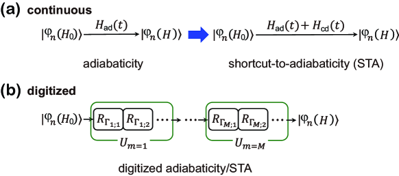
Figure 1: A schematic diagram of (a) continuous and (b) digitized adiabatic/STA processes.

For the STA process, a counter-diabatic Hamiltonian is introduced as BerryJPhysA09 ; XChenPRL2010 ; OdelinRMP19 ; TakahashiPRA17 ; ZhangSciRep16 ; ZZXPRA17 ; SCPMA2018 ; WangNJP2018 ; ZZXNJP2018 ; PWPRL19 ; chenxiPRAPP20 ; SantosJPAMT18 ; SmithNJP18 ; chenxiPRL10

$$H_{\mathrm{cd}}(t)=i\sum_{n}\left[|\dot{\varphi}_{n}(t)\rangle\langle\varphi_{n}(t)|-\langle\varphi_{n}(t)|\dot{\varphi}_{n}(t)\rangle|\varphi_{n}(t)\rangle\langle\varphi_{n}(t)|\right]$$ (2)

where $|\varphi_{n}(t)\rangle\equiv|\varphi_{n}(H_{\mathrm{ad}}(t))\rangle$ is the $n$-th instantaneous eigenstate of the adiabatic Hamiltonian $H_{\mathrm{ad}}(t)$. For a finite operation time $T$, the quantum system subject to the total Hamiltonian $H_{\mathrm{tot}}(t)\!=\!H_{\mathrm{ad}}(t)+H_{\mathrm{cd}}(t)$ is dragged exactly to the eigenstate $|\Psi(t\!=\!T)\rangle\!=\!U_{\mathrm{STA}}|\Psi(0)\rangle\!=\!\exp[i\Phi^{\prime}_{n}(T)]|\varphi_{n}(H)\rangle$ under the conditions of $\dot{\lambda}(0)\!=\!0$ and $\dot{\lambda}(T)\!=\!0$. The time evolution operator is changed to be $U_{\mathrm{STA}}=\exp_{+}[-i\int_{0}^{T}H_{\mathrm{tot}}(\tau)d\tau]$. Although the counter-diabatic Hamiltonian has been derived under various frameworks, e.g., the elimination of nonadiabatic transition BerryJPhysA09 ; XChenPRL2010 ; OdelinRMP19 ; TakahashiPRA17 ; ZhangSciRep16 ; ZZXPRA17 ; SCPMA2018 ; WangNJP2018 ; ZZXNJP2018 ; PWPRL19 ; chenxiPRAPP20 ; SantosJPAMT18 ; SmithNJP18 and the Lewis-Riesenfeld invariant chenxiPRL10 , $H_{\mathrm{cd}}(t)$ can recover the same expression in Eq. (2).

From the practical perspective, the adiabatic process usually needs a long operation time, i.e. $\varepsilon T_{\mathrm{min}}\gg 1$ with $\varepsilon$ a characteristic energy of the system and $T_{\mathrm{min}}$ the minimum value of $T$ for the output fidelity above a threshold. The STA can accelerate the adiabatic process but the appearance of instantaneous eigenstates in Eq. (2) contradicts our ultimate goal of determining $|\varphi_{n}(H)\rangle$. To avoid this problem, we apply a single-qubit assumption in the scenario of a weak inter-qubit interaction (see Appendix A and Sec. III for details) chenxiPRAPP20 . The operation time of this approximate STA can be compressed to satisfy $\varepsilon T_{\mathrm{min}}\lesssim O(1)$. With the increase of the inter-qubit interaction, a more systematic treatment is an expansion over nested commutators PWPRL19 , which requires a heavy computational cost as the expansion order increases. Instead, we re-select a more appropriate initial Hamiltonian $H_{0}$ to suppress the Hamiltonian deviation $\|H-H_{0}\|$ and the state distance between $|\varphi_{n}(H)\rangle$ and $|\varphi_{n}(H_{0})\rangle$. The adiabatic prediction is practically reliable under a short operation time [$\varepsilon T_{\mathrm{min}}\lesssim O(1)$] without the necessity of the STA.

The experimental realization of a time-varying multi-qubit Hamiltonian (adiabatic or STA) is possible but difficult. Instead, a digitized algorithm can realize the time evolution of an arbitrary Hamiltonian BarendsNat16 ; SteffenPRL03 ; LanyonSci11 ; SalathePRX15 ; chenxiPRAPP20 . After dividing the operation time into $M$ segments ($\Delta t\!=\!T/M$), we apply the Trotter-Suzuki decomposition BarendsNC15 ; LloydSci96 ; TrotterPAMS59 ; SuzukiCMP76 to the time evolution operator ($U=U_{\mathrm{ad}}$ or $U_{\mathrm{STA}}$), which leads to

$$U\!\approx\!U_{M}\cdots U_{2}U_{1}$$ (3)

with $U_{m=1,\cdots,M}\!=\!\exp[-iH_{\mathrm{ad/tot}}(m\Delta t)\Delta t]$. In general, the adiabatic or total Hamiltonian can be expanded into $H_{\mathrm{ad/tot}}(t)\!=\!\sum_{j=1}^{J}\omega_{j}(t)\Gamma_{j}/2$, where $\Gamma_{j}$ is a quantum operator, $\omega_{j}(t)$ is its associated coefficient and $J$ is the total number of operators. The Trotter-Suzuki decomposition allows a new factorization BarendsNC15 ; LloydSci96 ; TrotterPAMS59 ; SuzukiCMP76 ,

$$U_{m}\!\approx\!R_{\Gamma_{J}}(\theta_{m;J})\cdots R_{\Gamma_{2}}(\theta_{m;2})R_{\Gamma_{1}}(\theta_{m;1})$$ (4)

where $R_{\Gamma_{j}}(\theta_{m;j})\!=\!\exp[-i\theta_{m;j}\Gamma_{j}/2]$ can be viewed as a generalized rotation operator over an angle $\theta_{m;j}\!=\!\omega_{j}(m\Delta t)\Delta t$. In practice, $R_{\Gamma_{j}}(\theta_{m;j})$ can be realized by a combination of sequential single- and two-qubit gates. Notice that the real experimental time is determined by the total time of gates rather than the adiabatic or STA operation time $T$.

III EXPERIMENTAL realization

The digitized adiabatic and STA eigensolvers are implemented in a quantum computing device composed of six superconducting cross-shaped transmon qubits WangPRAPP2019 , from which two qubits ($Q_{A}$ and $Q_{B}$) are selected. The ground and excited states of each qubit are mapped onto the up and down states of a spin, i.e., $|0\rangle\!\leftrightarrow\!|+\rangle$ and $|1\rangle\!\leftrightarrow\!|-\rangle$. The device is mounted in an aluminum sample box and in a dilution refrigerator with a base temperature around 10 mK. The frequency-tunable qubits are initially biased at an operation point through two $Z$-control lines. In our experiment, the two qubits are set at $\omega_{A}/2\pi\!=\!6.21$ GHz and $\omega_{B}/2\pi\!=\!5.70$ GHz. The two anharmonicity parameters are $\Delta_{A}/2\pi\!\approx\!\Delta_{B}/2\pi\!=\!-250$ MHz, enabling a selective microwave drive to control each qubit through its $XY$-control line. At the operation point, the relaxation times are $T_{A;1}\!=\!5.8$ $\mu$s and $T_{B;1}\!=\!6.9$ $\mu$s while the pure dephasing times are $T_{A;\phi}\!=\!26$ $\mu$s and $T_{B;\phi}\!=\!28$ $\mu$s. The readout fidelities of the ground and the excited states are $F_{A;0}\!=\!99\%$ and $F_{A;1}\!=\!95\%$ for qubit $A$, and $F_{B;0}\!=\!97\%$ and $F_{B;1}\!=\!93\%$ for qubit $B$ XLPRAPP2020 .

III.1 Hydrogen Molecule

Under the Born-Oppenheim approximation, the electronic Hamiltonian of a hydrogen molecule is written as

$$H(\vec{r}_{1},\vec{r}_{2}|\vec{R}_{1},\vec{R}_{2}) = \mathcal{E}_{\mathrm{nucl}}(R)+\sum_{i=1,2}\frac{\vec{p}^{2}_{i}}{2m}-\sum_{i,j=1,2}\frac{e^{2}}{4\pi\varepsilon_{0}|\vec{r}_{i}-\vec{R}_{j}|}+\frac{e^{2}}{4\pi\varepsilon_{0}|\vec{r}_{1}-\vec{r}_{2}|},$$ (5)

where $\vec{p}_{i=1,2}$ and $\vec{r}_{i=1,2}$ are the momentums and coordinates of two electrons, and $\vec{R}_{i=1,2}$ are the coordinates of two nuclei. The nuclear term $\mathcal{E}_{\mathrm{nucl}}(R)$ is dependent on the internuclear distance $R=|\vec{R}_{1}-\vec{R}_{2}|$. For the ground and several lowest excited electronic states of H₂, the single-electron basis functions are combined by two delocalized orbitals $\{|\phi_{g}\rangle,|\phi_{u}\rangle\}$ and two spin states $\{|+\rangle,|-\rangle\}$, i.e., $|\chi_{i=1,\cdots,4}(\vec{r},\sigma)\rangle\!=\!|\phi_{g/u}(\vec{r})\rangle\otimes|\sigma\!=\!+/-\rangle$ with $\vec{r}$ and $\sigma$ the coordinate and spin variables PeruzzoNC14 ; MalleyPRX16 ; CollessPRX18 . In the number representation with regard to $\{|\chi_{i}\rangle\}$, the second quantization of the Hamiltonian is $H=\mathcal{E}_{\mathrm{nucl}}+\sum h_{ij}a^{+}_{i}a_{j}+\sum h_{ijkl}a^{+}_{i}a^{+}_{j}a_{k}a_{l}$, where $a_{i}$ and $a^{+}_{i}$ are annihilation and creation operators satisfying $[a_{i},a^{+}_{j}]_{+}=\delta_{i,j}$. The single- and two-electron integrals ($h_{ij}$ and $h_{ijkl}$) depend on the internuclear distance $R$ PeruzzoNC14 ; MalleyPRX16 ; CollessPRX18 . As shown in Appendix B, the Bravyi-Kitaev transformation SeeleyJCP01 is applied and the target Hamiltonian is approximated as

$$H=g_{0}+gZ_{A}+gZ_{B}+g_{12}Y_{A}Y_{B},$$ (6)

where $\{X_{\alpha},Y_{\alpha},Z_{\alpha}\}$ is the set of Pauli matrices ($\alpha=A,B$), and the parameters $\{g_{0},g,g_{12}\}$ are functions of $R$ PeruzzoNC14 ; MalleyPRX16 ; CollessPRX18 .

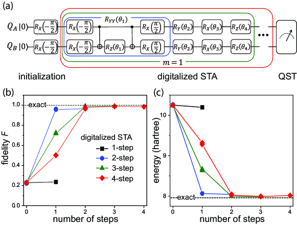
Figure 2: Determination of the ground state of H₂ via a digitized STA eigensolver for the internuclear distance at $R=0.05$ Å. (a) A quantum circuit diagram of the $M$-step digitized STA process. (b) The evolution of the state fidelities (in comparison to the exact ground state) in four digitized STA experiments ($1\leq M\leq 4$). (c) The evolution of the state energies in four digitized STA experiments. The square, circle, triangle and diamond stand for the total number $M=1,2,3,4$ of digitized steps, respectively.

In the first step, we explore the ground state $|\varphi_{0}(H)\rangle$ at $R=0.05$ Å, where the energy parameters are $g_{0}\!=\!10.08~{}E_{\mathrm{h}}$, $g\!=\!-1.055~{}E_{\mathrm{h}}$ and $g_{12}\!=\!0.1557~{}E_{\mathrm{h}}$ ($E_{\mathrm{h}}\!\approx\!27.2$ eV) CollessPRX18 . The initial Hamiltonian is selected to be $H_{0}=g(Y_{A}+Y_{B})$ and the adiabatic Hamiltonian $H_{\mathrm{ad}}(t)=H_{0}+\lambda(t)(H-H_{0})$ is given by Eq. (1). The time-adjusting coefficient is set to be $\lambda(0\leq t\leq T)=\sin^{2}(\pi t/2T)$ and this form is applied to all the experiments and numerical simulations in this paper. The initial ground state $|\varphi_{0}(H_{0})\rangle=(|0\rangle+i|1\rangle)_{A}(|0\rangle+i|1\rangle)_{B}/2$ is experimentally generated by applying the $R_{X_{A}}(-\pi/2)$ and $R_{X_{B}}(-\pi/2)$ gates onto the two-qubit state $|00\rangle$. Due to the condition of $|g_{12}|\!\ll\!|g|$, the two-qubit coupling is separated into $Y_{A}Y_{B}\approx Y_{A}+Y_{B}$ under the single-qubit approximation (see Appendix A) chenxiPRAPP20 . Accordingly, the counter-diabatic Hamiltonian is approximated as $H_{\mathrm{cd}}(t)\approx g_{\mathrm{cd}}(t)(X_{A}+X_{B})$ with $g_{\mathrm{cd}}(t)=\dot{\lambda}(t)/[2\zeta^{2}(t)+2\lambda^{2}(t)]$ and $\zeta(t)=1-(1-g_{12}/g)\lambda(t)$. With both the adiabatic part $H_{\mathrm{ad}}(t)$ and the counter-diabatic part $H_{\mathrm{cd}}(t)$, the total Hamiltonian is organized into

$$H_{\mathrm{tot}}(t) \approx \lambda(t)g_{0}+\frac{\omega_{1}(t)}{2}Y_{A}Y_{B}+\frac{\omega_{2}(t)}{2}(Y_{A}+Y_{B})$$ (7)

$$+\frac{\omega_{3}(t)}{2}(X_{A}+X_{B})+\frac{\omega_{4}(t)}{2}(Z_{A}+Z_{B}),$$

with $\omega_{1}(t)=2\lambda(t)g_{12}$, $\omega_{2}(t)=2[1-\lambda(t)]g$, $\omega_{3}(t)=2g_{\mathrm{cd}}(t)$ and $\omega_{4}(t)=2\lambda(t)g$. The STA operation time is empirically selected at $gT\approx 0.8$, which is much shorter than that for an adiabatic process ($gT_{\mathrm{min}}\approx 9$). The whole time evolution of the $M$-step digitized STA is given by Eq. (3) and each $m$-th partial time evolution operator is set to be

$$U_{m} = R_{Z_{A}}(\theta_{m;4})R_{Z_{B}}(\theta_{m;4})R_{X_{A}}(\theta_{m;3})R_{X_{B}}(\theta_{m;3})$$ (8)

$$\times R_{Y_{A}}(\theta_{m;2})R_{Y_{B}}(\theta_{m;2})R_{Y_{A}Y_{B}}(\theta_{m;1}),$$

with

$$\left\{\begin{array}[]{cclcl}\theta_{m,1}&=&2\lambda(m\Delta t)g_{12}\Delta t\\ \theta_{m,2}&=&2[1-\lambda(m\Delta t)]g\Delta t\\ \theta_{m,3}&=&2g_{\mathrm{cd}}(m\Delta t)\Delta t\\ \theta_{m,4}&=&2\lambda(m\Delta t)g\Delta t\end{array}\right..$$ (13)

The two-qubit rotation $R_{Y_{A}Y_{B}}(\theta)$ in Eq. (8) is experimentally realized by BarendsNC15

$$R_{Y_{A}Y_{B}}(\theta)=R_{X_{A}}(\pi/2)R_{X_{B}}(\pi/2)U_{\mathrm{CN}}R_{Z_{B}}(\theta)U_{\mathrm{CN}}R_{X_{A}}(-\pi/2)R_{X_{B}}(-\pi/2),$$ (14)

where $U_{\mathrm{CN}}$ stands for a two-qubit CNOT gate. The corresponding pulse sequence is shown in Fig. 2(a). In practice, we perform the digitized STA experiment up to four steps ($1\!\leq\!M\!\leq\!4$).

In our experiment on superconducting qubits, errors occur during the initialization, operation and measurement. For example, the input pulse is generated by a digital-analog-converter (DAC) so that the pulse experienced by qubits can deviate from the designed shape due to the filtering effect. A single STA step in Eq. (8) involves 11 single-qubit gates and 2 two-qubit gates and the operation error can quickly accumulate through an $M$-step STA process. Due to the nature of a transmon qubit, the error is unavoidable in the state measurement. In addition to a careful calibration, we introduce three approaches to further correct errors and achieve a reliable output. (1) At each $m$-th step, the starting state $|\Psi((m-1)\Delta t)\rangle$ is re-prepared by a two-qubit universal quantum circuit (4 rotation gates and 1 CNOT gate) ShendePRA03 after it is experimentally determined in the previous $(m-1)$-th step. Our modification is equivalent to an evolution of $|\Psi(0)\rangle\rightarrow|\Psi((m-1)\Delta t)\rangle\rightarrow|\Psi(m\Delta t)\rangle$, which can largely suppress the error accumulation in the pathway of $|\Psi(0)\rangle\rightarrow|\Psi(\Delta t)\rangle\rightarrow\cdots\rightarrow|\Psi((m-1)\Delta t)\rangle$. For an $N(>2)$-qubit system, the universal quantum circuit can become difficult but a single-step production of $|\Psi(0)\rangle\rightarrow|\Psi((m-1)\Delta t)\rangle$ is practically possible. In the VQE protocol, the state determination of $|\Psi(0)\rangle\rightarrow|\Psi(H)\rangle$ is a single-step operation although the rotation angles vary step by step PeruzzoNC14 ; MalleyPRX16 ; KandalaNat17 ; GoogleSci20 ; CollessPRX18 . (2) At each $m$-th step, the rotation angles $\{\theta_{m;j}\}$ in Eq. (13) are adjusted to improve the reliability of $U_{m}$ since the overall effect of various errors behaves as a ‘phase error’ in our generalized rotation operators. The angle adjustment is in general a small value ($\lesssim 5^{\circ}$) around its theoretical design, and a similar experimental technique can be found in a previous VQE experiment of the hydrogen molecule MalleyPRX16 . (3) Due to the limitation of our current experimental setup, the previous two approaches cannot fully remove the errors so that we apply a state purification approach as follows. For an arbitrary mixed state, the density matrix can be diagonalized and expanded into $\rho_{\mathrm{exp}}(t)=\sum_{i}P_{i}(t)|\psi_{i}(t)\rangle\langle\psi_{i}(t)|$, where $|\psi_{i}(t)\rangle$ is a pure state and $P_{i}(t)$ is its population. We expect that the state evolution is not far away from the theoretical simulation. The state $|\psi_{i}(t)\rangle$ with the largest population is thus considered to be an error-corrected experimental result. To visualize the influence of the error correction, we sequentially measure the starting and ending density matrices, $\rho((m-1)\Delta t)$ and $\rho(m\Delta t)$, with the quantum state tomography (QST). Next we calculate a fidelity function,

$$\mathcal{S}=\langle\Psi_{\mathrm{theo}}(t)|\rho_{\mathrm{exp}}(t)|\Psi_{\mathrm{theo}}(t)\rangle,$$ (15)

between the experimental result $\rho_{\mathrm{exp}}(t)$ and the theoretical simulation $|\Psi_{\mathrm{theo}}(t)\rangle\langle\Psi_{\mathrm{theo}}(t)|$ at the starting time $t=(m-1)\Delta t$ and the ending time $t=m\Delta t$. The propagation results of $\mathcal{S}$ for the $M$-step digitized STA ($1\leq M\leq 4$) are shown in Fig. 3. Except for $|\Psi(0)\rangle$, the starting state $|\Psi((m-1)\Delta t)\rangle$ generated by the universal quantum circuit exhibits a $\sim 5\%$ error, and a one-step digitized STA results in an extra $5\%\sim 10\%$ error for the ending state $|\Psi(m\Delta t)\rangle$. After the purification, the state fidelities of $\mathcal{S}$ are consistently improved to be $>99\%$. The above three treatments are also used in other experiments in this paper, but may be unnecessary with the future improvement of sample quality and control accuracy.

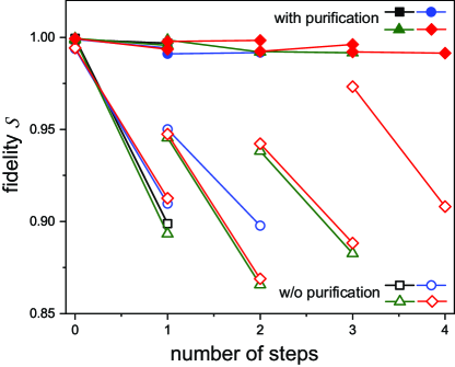
Figure 3: The fidelity of the experimental density matrix $\rho_{\mathrm{exp}}(t)$ in comparison to the theoretical simulation $|\Psi_{\mathrm{theo}}(t)\rangle\langle\Psi_{\mathrm{theo}}(t)|$ for the experiment shown in Fig. 2. The open symbols represent the results without the state purification. The solid symbols represent the results by selecting the pure state $|\psi_{i}(t)\rangle$ with the largest population after the diagonalization of $\rho_{\mathrm{exp}}(t)$. The square, circle, triangle and diamond stand for the total number $M=1,2,3,4$ of digitized steps, respectively.

Next we present the time evolution of the error-corrected experimental result $|\Psi(t\!=\!m\Delta t)\rangle$ in comparison to the exact ground state $|\varphi_{0}(H)\rangle$. Similarly, another fidelity function,

$$\mathcal{F}_{m}\!=\!|\langle\varphi_{0}(H)|\Psi(t\!=\!m\Delta t)\rangle|^{2},$$ (16)

is introduced for a quantitative description, and the experimental results of $\mathcal{F}_{m}$ are presented in Fig. 2(b). For $M\geq 2$, the digitized STA efficiently drags the initial state ($\mathcal{F}_{0}=23\%$) to the exact state (the best fidelity $\mathcal{F}_{M}\!\approx\!99\%$). We also calculate the state energies $E_{m}\!=\!\langle\Psi(m\Delta t)|H|\Psi(m\Delta t)\rangle$ through each $M$-step process [see Fig. 2(c)], the experimental extraction is almost the same as the exact value $\varepsilon_{0}(R\!=\!0.05~{}\mathrm{\AA})\!=\!7.96$ $E_{\mathrm{h}}$.

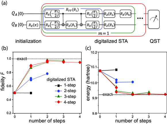
Figure 4: Determination of the first excited state of H₂ via a digitized STA eigensolver for the internuclear distance at $R=0.05$ Å. (a) A quantum circuit diagram of the $M$-step digitized STA process. (b) The evolution of the state fidelities in four digitized STA experiments ($1\leq M\leq 4$) in comparison with the exact result. (c) The evolution of the state energies in four digitized STA experiments. The square, circle, triangle and diamond stand for the total number $M=1,2,3,4$ of digitized steps, respectively.

In the second step, we explore the first excited state $|\varphi_{n=1}(H)\rangle$ at $R\!=\!0.05~{}\mathrm{\AA}$ while the other two excited states can be investigated similarly. The initial Hamiltonian is changed to be $H_{0}\!=\!gZ_{A}$, and the initial state $|\Psi(0)\rangle\!=\!|01\rangle$ is obtained by applying the $R_{X_{B}}(\pi)$-gate onto the state $|00\rangle$. Following the same procedure as above, a short operation time is selected at $gT\approx 4.0$ and each $m$-th partial time evolution operator in the digitized STA is given by

$$U_{m}=R_{X_{A}}(\theta_{m;4})R_{Z_{A}}(\theta_{m;3})R_{Z_{B}}(\theta_{m;2})R_{Y_{A}Y_{B}}(\theta_{m;1}).$$ (17)

with

$$\left\{\begin{array}[]{cclcl}\theta_{m,1}&=&2\lambda(m\Delta t)g_{12}\Delta t\\ \theta_{m,2}&=&2g\Delta t\\ \theta_{m,3}&=&2\lambda(m\Delta t)g\Delta t\\ \theta_{m,4}&=&2g_{\mathrm{cd}}(m\Delta t)\Delta t\end{array}\right.$$ (22)

and $g_{\mathrm{cd}}(t)=-\dot{\lambda}(t)gg_{12}/[2g+2g_{12}\lambda^{2}(t)]$. The corresponding pulse sequence is plotted in Fig. 4(a). The experimental results of the state fidelity $\mathcal{F}_{m}\!=\!|\langle\varphi_{n=1}(H)|\Psi(m\Delta t)\rangle|^{2}$ and the state energy $E_{m}$ are presented in Figs. 4(b) and 4(c). Consistent with the behavior in the ground state, the digitized STA efficiently drags the initial state ($\mathcal{F}_{0}\!=\!50\%$) to the exact first excited state (the best fidelity $\mathcal{F}_{M}\!\approx\!98\%$) for $M\!\geq\!3$, leading to an excellent prediction of the eigenenergy at $\varepsilon_{1}(R\!=\!0.05~{}\mathrm{\AA})\!=\!9.92$ $E_{\mathrm{h}}$.

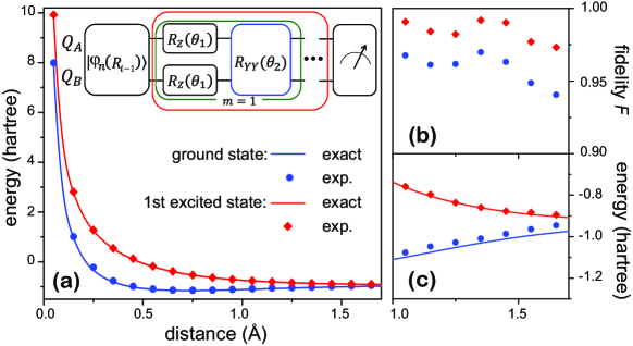
Figure 5: Experimental determination of the potential energy landscapes for both the ground and excited states of H₂ via the digitized STA and sequential digitized adiabatic eigensolvers. (a) The two eigenergies ($\varepsilon_{n=0,1}$) as the functions of the internuclear distance $R$. The quantum circuit diagram of a sequential digitized adiabaticity is shown in the inset. In the large-distance range ($1.05~{}\mathrm{\AA}\!\leq\!R\!\leq\!1.65~{}\mathrm{\AA}$), the experimental results of the state fidelities and eigenenergies are enlarged in (b) and (c). The symbols (circles and diamonds) represent the experimental results while the solid lines represent the exact results from the theoretical calculation.

In the final step, we explore the electronic states of H₂ for various internuclear distances $R$, i.e., $|\varphi_{n=0,1}(R)\rangle\!\equiv\!|\varphi_{n=0,1}(H(R))\rangle$. With the increase of $R$, the amplitude of $g(R)$ gradually decreases and eventually becomes smaller than $g_{12}(R)$. For the two initial Hamiltonians, $H_{0}=g(Y_{A}+Y_{B})$ and $H_{0}=gZ_{A}$, the previous single-qubit approximation gradually fails. Instead of an expansion over nested commutators PWPRL19 , we apply a sequential digitized adiabatic approach. In the range of $0.05~{}\mathrm{\AA}\!\leq\!R\!\leq\!1.65~{}\mathrm{\AA}$, a sequence of the internuclear distances is set as $\{R_{0}=0.05~{}\mathrm{\AA},R_{1}=0.15~{}\mathrm{\AA},\cdots,R_{16}=1.65~{}\mathrm{\AA}\}$, which satisfies $R_{i}\!=\!R_{i-1}+\Delta R$ and $\Delta R=0.1~{}\mathrm{\AA}$. To obtain the electronic structure at the $i$-th distance, the initial Hamiltonian is selected to be $H_{0}=c(R_{i})H(R_{i-1})$ with $c(R_{i})=g_{12}(R_{i})/g_{12}(R_{i-1})$ and the initial states are the corresponding ground and first excited states, $|\Psi(0)\rangle\!=\!|\varphi_{n=0,1}(R_{i-1})\rangle$, which have been determined at the previous $(i-1)$-th distance. The adiabatic Hamiltonian is given accordingly by $H_{\mathrm{ad}}(t)=c(R_{i})H(R_{i-1})+\lambda(t)[H(R_{i})-c(R_{i})H(R_{i-1})]$. Due to a relatively small deviation between $|\varphi_{n}(R_{i-1})\rangle$ and $|\varphi_{n}(R_{i})\rangle$, the adiabatic evolution can converge quickly and we practically choose a digitized adiabatic process to realize the eigensolver. In detail, the time evolution operator of the digitized adiabaticity is set to be $U_{\mathrm{ad}}\!=\!U_{M}\cdots U_{m}\cdots U_{1}$ and

$$U_{m=1,\cdots,M}=R_{Y_{A}Y_{B}}(\theta_{m;2})R_{Z_{A}}(\theta_{m;1})R_{Z_{B}}(\theta_{m;1}).$$ (23)

The rotation angles are $\theta_{m;1}=2g_{\lambda}(m\Delta t)\Delta t$ and $\theta_{m;2}=2g_{12}(R_{i})\Delta t$ where we introduce a function, $g_{\lambda}(t)\!=\!\lambda(t)g(R_{i})\!+\![1\!-\!\lambda(t)]c(R_{i})g(R_{i-1})$. The pulse sequence of this digitized adiabatic evolution is shown in the inset of Fig. 5(a). The operation time is in the range of $1.0\leq gT\leq 1.6$. For the ground state $|\varphi_{0}(R_{i})\rangle$, the number of digitized steps are $M=2$ for $0.15~{}\mathrm{\AA}\!\leq\!R_{i}\!\leq\!1.05~{}\mathrm{\AA}$ and $M=5$ for $1.15~{}\mathrm{\AA}\!\leq\!R_{i}\!\leq\!1.65~{}\mathrm{\AA}$. For the first excited state $|\varphi_{1}(R_{i})\rangle$, the number of digitized steps is always $M=2$. To reduce the accumulation of experimental errors, the initial states $|\varphi_{n}(R_{i-1})\rangle$ are re-prepared according to the numerical simulation result (including a systematic error from the sequential digitized adiabaticity) with the universal quantum circuit ShendePRA03 . The experimental result of the sequential digitized adiabaticity is summarized in Fig. 5(a)-5(c). In the most relevant range around the equilibrium distance, the state fidelities of both the ground and first excited states satisfy $\mathcal{F}_{M}\gtrsim 98\%$. In the range of large distances ($1.05~{}\mathrm{\AA}\!\leq\!R_{i}\!\leq\!1.65~{}\mathrm{\AA}$), the fidelity of the ground state is $\mathcal{F}_{M}\gtrsim 94\%$ while that of the first excited state is $\mathcal{F}_{M}\gtrsim 97\%$ [see Fig. 5(b)]. The fidelity drop is expected to slow down with the decrease of the distance deviation $\Delta R$. The potential energy landscape extracted experimentally is plotted in Fig. 5(a), showing an excellent agreement with the theoretical prediction. An enlarged view of the energy landscape for $1.05~{}\mathrm{\AA}\!\leq\!R_{i}\!\leq\!1.65~{}\mathrm{\AA}$ is shown in Fig. 5(c). We thus obtain an accurate description of the electronic structure of H₂ using a delicate and efficient design of the digitized STA and the sequential digitized adiabaticity.

III.2 Topological BHZ model

The BHZ model can be used to describe the quantum spin Hall effect in a two-dimensional square lattice (the lattice constant is $a$) ZhangSci06 . For simplicity, we consider one $s$-orbital and one $p$-orbital at each lattice point. In addition to the intra-orbital interactions, the spin-modulated and orientation-modulated inter-orbital interactions are included for the nearest neighbor hopping. After a discrete Fourier transform, the tight-binding Hamiltonian in the momentum space is block diagonal against the wavevector $\vec{k}$, giving $H=\sum_{\vec{k}}H(\vec{k})$ and

$$H(\vec{k})=\sum_{\gamma_{1}=s,p}\sum_{\gamma_{2}=s,p}\sum_{\sigma=\pm}|\vec{k}\gamma_{1}\sigma\rangle[H(\vec{k})]_{\gamma_{1}\sigma;\gamma_{2}\sigma}\langle\vec{k}\gamma_{2}\sigma|.$$ (24)

By mapping the two orbitals $\{|s\rangle,|p\rangle\}$ onto a two-state spin, Eq. (24) is reorganized into

$$H(\vec{k})=g_{0}(\vec{k})+g(\vec{k})Z_{B}+\left[g_{12}(k_{x})X_{B}+g_{12}(k_{y})Y_{B}\right]Z_{A},$$ (25)

where the subscripts $A$ and $B$ denote the spin and orbital degrees of freedoms, respectively. The coefficients are explicitly given by

$$\left\{\begin{array}[]{ccl}g_{0}(\vec{k})&=&C_{1}f(\vec{k})\\ g(\vec{k})&=&C_{2}f(\vec{k})-C_{3}\\ g_{12}(h=k_{x},k_{y})&=&C_{4}\sin(ha)\end{array}\right.$$ (29)

with $f(\vec{k})=8[\sin^{2}(k_{x}a/2)\!+\!\sin^{2}(k_{y}a/2)]$. In our experiment, the three parameters are set to be $C_{1}=0.020$ eV, $C_{2}=0.027$ eV, $C_{3}=0.055$ eV and $C_{4}=0.073$ eV from the HgTe/CdTe semiconductor quantum well JiangPRB09 . The symmetry of $H$ indicates two-fold degenerate energy bands and a Dirac point at the $\Gamma$-point ($k_{x}\!=\!k_{y}\!=\!0$) of the first Brillouin zone (FBZ). To demonstrate the reliability of the digitized STA and the sequential digitized adiabaticity, we drive the two-qubit system to determine the valence and conduction bands along the X-$\Gamma$-X linecut ($-\pi\!\leq\!k_{x}a\!<\!\pi$ and $k_{y}\!=\!0$) in the FBZ.

Similar to the treatment in H₂, we first explore the electronic states $|\varphi_{n=0,1}(k_{x_{0}})\rangle\!\equiv\!|\varphi_{n}(H(k_{x}\!=\!k_{x_{0}},k_{y}\!=\!0))\rangle$ at two sets of starting points: one near the $\Gamma$-point ($k_{x_{0}}\!=\!\pm 0.1a^{-1}$) and the other near the X-point ($k_{x_{0}}\!=\!\pm 3.1a^{-1}$). For each wavevector, the initial Hamiltonian is selected to be $H_{0}=g(k_{x_{0}})Z_{B}$. The initial ground state of $H_{0}$ is $|\varphi_{0}(H_{0})\rangle\!=\!|01\rangle$, generated by the $R_{X_{B}}(\pi)$ gate onto the two-qubit state $|00\rangle$, while the initial excited state is $|\varphi_{1}(H_{0})\rangle\!=\!|00\rangle$. With respect to the adiabatic Hamiltonian, $H_{\mathrm{ad}}(t)=H_{0}+\lambda(t)(H-H_{0})$, the counter-diabatic Hamiltonian $H_{\mathrm{cd}}(t)$ is obtained under the single-qubit approximation, which is valid with the consideration of $|g_{12}(k_{x_{0}})|\ll|g(k_{x_{0}})|$. In the $M$-step digitized STA, the partial time evolution operator at each step is given by

$$U_{m} = R_{Z_{B}}(\theta_{m;3})R_{Y_{B}}(\theta_{m;2})R_{Z_{A}X_{B}}(\theta_{m;1}).$$ (30)

with

$$\left\{\begin{array}[]{ccl}\theta_{m;1}&=&2\lambda(m\Delta t)g_{12}(k_{x_{0}})\Delta t\\ \theta_{m;2}&=&2g_{\mathrm{cd}}(k_{x_{0}};m\Delta t)\Delta t\\ \theta_{m;3}&=&2g(k_{x_{0}})\Delta t\end{array}\right.$$ (34)

and $g_{\mathrm{cd}}(k_{x_{0}};t)=\dot{\lambda}(t)g(k_{x_{0}})g_{12}(k_{x_{0}})/[2g(k_{x_{0}})+2g_{12}(k_{x_{0}})\lambda^{2}(t)]$. The corresponding pulse sequences for both the ground and excited states are shown in Figs. 6(a) and 6(b), respectively. In practice, we perform eight 4-step digitized STA experiments ($0.5\leq gT\leq 0.6$) and determine the corresponding eigenstates. For both $k_{x_{0}}\!=\!\pm 0.1a^{-1}$ and $\pm 3.1a^{-1}$, the experimental state fidelities of $|\varphi_{n=0,1}(k_{x_{0}})\rangle$ are around $98\%\sim 99\%$.

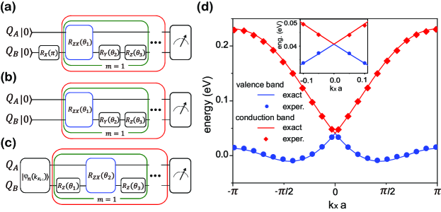
Figure 6: Experiment of the BHZ model. (a) and (b) The quantum circuit diagrams of the digitized STA to determine the ground and excited eigenstate at the starting wavevectors, $k_{x_{0}}=\pm 0.1a^{-1},\pm 3.1a^{-1}$. (c) The quantum circuit diagram of the sequential digitized adiabaticity for other wavevectors, $k_{x}\neq k_{x_{0}}$. (d) The experimental determination of the valence and conduction bands along the X-$\Gamma$-X linecut. Inset is an enlarged view of (d) around the Dirac point. The symbols (circles and diamonds) represent the experimental results while the solid lines represent the exact results from the theoretical calculation.

Next we explore the electronic states $|\varphi_{n=0,1}(k_{x})\rangle$ at different wavevectors along the X-$\Gamma$-X linecut through the sequential digitized adiabaticity. With respect to each starting wavevector ($k_{x_{0}}=\pm 0.1a^{-1},\pm 3.1a^{-1}$), a sequence of wavevectors, $\{k_{x_{0}},k_{x_{1}},\cdots,k_{x_{i}},\cdots\}$, is assigned. For each sequence, the ending wavector is at $k_{x}=\pm 1.6a^{-1}$ and the wavevector deviation is $\Delta k_{x}=\pm 0.3a^{-1}$. In addition, we investigate two small wavevectors, $k_{x}=\pm 0.05a^{-1}$, using the reference points at $k_{x_{0}}=\pm 0.1a^{-1}$. At each $i$-th wavevector $k_{x_{i}}$, the initial Hamiltonian is set to be $H_{0}=c(k_{x_{i}})H(k_{x_{i-1}})$ with $c(k_{x_{i}})=g_{12}(k_{x_{i}})/g_{12}(k_{x_{i-1}})$, while the initial state is $|\Psi(0)\rangle\!=\!|\varphi_{n=0,1}(k_{x_{i-1}})\rangle$. The adiabatic Hamiltonian is given by $H_{\mathrm{ad}}(t)=c(k_{x_{i}})H(k_{x_{i-1}})+\lambda(t)[H(k_{x_{i}})-c(k_{x_{i}})H(k_{x_{i-1}})]$. In the $M$-step digitized adiabatic process, each partial time evolution operator is given by

$$U_{m}=R_{Z_{B}}(\theta_{m;3})R_{Z_{A}X_{B}}(\theta_{m;2})R_{Z_{B}}(\theta_{m;1})$$ (35)

with $\theta_{m;1}=2\Delta g(k_{x_{i}})\lambda(m\Delta t)\Delta t$, $\theta_{m;2}=2g_{12}(k_{x_{i}})\Delta t$ and $\theta_{m;3}=2c(k_{x_{i}})g(k_{x_{i-1}})\Delta t$. Here we introduce a deviation function, $\Delta g(k_{x_{i}})\!=\!g(k_{x_{i}})\!-\!c(k_{x_{i}})g(k_{x_{i-1}})$. The pulse sequence of the digitized adiabaticity is shown in the inset of Fig. 6(c). The separation of $R_{Z_{B}}(\theta_{1})$ and $R_{Z_{B}}(\theta_{3})$ in Eq. (35) is found to yield a better performance than the combined case. The operation times are selected in the range of $0.4\leq gT\leq 1.8$. For $|k_{x}|\!\leq\!1.0a^{-1}$, the number of adiabatic steps is $M=2$, while for $1.3a^{-1}\!\leq\!|k_{x}|\!\leq\!2.8a^{-1}$, this number is changed to be $M=5$. The experimental state fidelities of both the valence and conduction bands along the X-$\Gamma$-X linecut satisfy $\mathcal{F}_{M}\gtrsim 98\%$. In Fig. 6(d), we plot the corresponding experimental band structures, $\varepsilon_{n=0,1}(k_{x})\!=\!\langle\varphi_{n}(k_{x})|H|\varphi_{n}(k_{x})\rangle$, which agrees excellently with the theoretical prediction. In the inset of Fig. 6(d), we experimentally extract a linear dispersion relation, $\varepsilon_{n}(k_{x})-2C_{1}\!\sim\!\pm C_{4}k_{x}a$ around the Dirac point ($k_{x}\!=\!0$).

IV Numerical Simulation of Hydrogen Chains

Our experiments of the two-atom hydrogen molecule and the BHZ model have revealed the applicability of the digitized STA followed by the sequential digitized adiabaticity in the determination of electronic states. Next we investigate the ground state for $N(>2)$-atom hydrogen chains GoogleSci20 . Due to the restriction of our current setup, it is difficult for us to reliably perform an $N(>2)$-qubit experiment. Therefore, we only present the results of numerical simulation in this paper and the experimental implementation will be performed in the future.

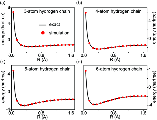
Figure 7: The ground state energy landscapes of the 3-, 4-, 5- and 6-atom hydrogen chains, where $R$ is the internuclear distance between two adjacent atoms. The red circles are obtained from the numerical simulation of the digitized STA and the sequential digitized adiabaticity while the black solid lines are the exact results.

The Hamiltonian of an $N$-atom hydrogen chain is written as

$$H(N;R)=g_{0}(R)+\sum_{i=1}^{N}g(R)Z_{i}+\sum_{i=1}^{N-1}g_{12}(R)Y_{i}Y_{i+1},$$ (36)

where $R$ is the internuclear distance between each pair of two adjacent hydrogen atoms. For simplicity, the $R$-dependencies of $g_{0}(R)$, $g(R)$ and $g_{12}(R)$ are assumed to be the same as those in the two-atom hydrogen molecule. (1) For the specified distance ($R\!=\!R_{0}\!=\!0.05$ Å), the initial Hamiltonian is set to be $H_{0}=H(N-1;R_{0})+g(R_{0})Z_{N}$ and the adiabatic Hamiltonian reads $H_{\mathrm{ad}}(t)\!=\!H(N-1;R_{0})+g(R_{0})Z_{N}+\lambda(t)g_{12}(R_{0})Y_{N-1}Y_{N}$. The initial state is set to be $|\Psi(0)\rangle=|\varphi_{0}(N-1;R_{0})\rangle\otimes|0\rangle$, where the ground state $|\varphi_{0}(N-1;R_{0})\rangle$ of the $(N-1)$-atom chain is predetermined. The adiabatic process is digitized into

$$U_{m}=R_{Y_{1}Y_{2}}(\theta_{m;3})\cdots R_{Y_{N-2}Y_{N-1}}(\theta_{m;3})R_{Y_{N-1}Y_{N}}(\theta_{m;2})R_{Z_{1}}(\theta_{m;1})\cdots R_{Z_{N}}(\theta_{m;1})$$ (37)

with $\theta_{m;1}=2g(R_{0})\Delta t$, $\theta_{m;2}=2g_{12}(R_{0})\lambda(m\Delta t)\Delta t$ and $\theta_{m;3}=2g_{12}(R_{0})\Delta t$. (2) For the other distances ($R>R_{0}$), a sequential digitized adiabatic protocol is applied onto the same distance sequence, $\{R_{0}=0.05~{}\mathrm{\AA},R_{1}=0.15~{}\mathrm{\AA},\cdots,R_{16}=1.65~{}\mathrm{\AA}\}$, as in Sec. III.1. At each $i$-th distance, the initial Hamiltonian is selected to be $H_{0}=c(R_{i})H(N;R_{i-1})$ and the adiabatic Hamiltonian is given accordingly by $H_{\mathrm{ad}}(t)=c(R_{i})H(N;R_{i-1})+\lambda(t)[H(N;R_{i})-c(R_{i})H(N;R_{i-1})]$. The initial state $|\varphi_{0}(N;R_{i-1})\rangle$ is predetermined at the previous $(i-1)$-th distance. For the digitized adiabatic operator, $U_{\mathrm{ad}}\!=\!U_{M}\cdots U_{m}\cdots U_{1}$, each partial time evolution is given by

$$U_{m}=R_{Y_{1}Y_{2}}(\theta_{m;2})\cdots R_{Y_{N-1}Y_{N}}(\theta_{m;2})R_{Z_{1}}(\theta_{m;1})\cdots R_{Z_{N}}(\theta_{m;1})$$ (38)

with $\theta_{m;1}=2g_{\lambda}(m\Delta t)\Delta t$ and $\theta_{m;2}=2g_{12}(R_{i})\Delta t$. The adiabatic operation time is in the range of $0.1\leq gT\leq 0.9$ while the number of the digitized steps is in the range of $3\leq M\leq 10$. In general, the value of $M$ increases with the increase of the chain length $N$ and the internuclear distance $R$. The ground state energy landscapes ($\varepsilon_{0}$ versus $R$) obtained for the $N$-atom hydrogen chains ($3\!\leq\!N\!\leq\!6$) are plotted in Figs. 7(a)-7(d). Through a series of sequential numerical simulations from the 3- to 6-atom chains, we successfully determine the structure of the electronic ground states. The state fidelities from the numerical simulation are $\gtrsim 99\%$ at short internuclear distances and still $\gtrsim 95\%$ for $1.05~{}\mathrm{\AA}\!\leq\!R_{i}\!\leq\!1.65~{}\mathrm{\AA}$.

V Summary

In this paper, we apply an eigensolver of the digitized STA and the sequential digitized adiabaticity to determine the electronic states of various systems. For the two-atom hydrogen molecule and the topological BHZ model, the state determination is experimentally implemented in a two-qubit superconducting device. (1) In the case of the hydrogen molecule, we select an internuclear distance at $R=R_{0}=0.05~{}\mathrm{\AA}$ with a weak inter-qubit interaction. Two uncoupled Hamiltonians are set to be the initial Hamiltonians $H_{0}$ and the counter-diabatic Hamiltonians $H_{\mathrm{cd}}(t)$ are estimated under the single-qubit assumption. Both the ground ($|\varphi_{0}(R=R_{0})\rangle$) and first excited ($|\varphi_{1}(R=R_{0})\rangle$) states are experimentally determined by the 4-step digitized STA (state fidelities $\mathcal{F}\approx 99\%$ and $98\%$). Subsequently, we set a sequence of internuclear distances, $\{R_{0}=0.05~{}\mathrm{\AA},R_{1}=0.15~{}\mathrm{\AA},\cdots,R_{16}=1.65~{}\mathrm{\AA}\}$. For each $i$-th distance $R_{i}$, the initial Hamiltonian is set to be $H(R_{i-1})$ at the $(i-1)$-th distance. With the initial states at $|\varphi_{0}(R_{i-1})\rangle$ and $|\varphi_{1}(R_{i-1})\rangle$, a $M$-step digitized adiabatic process is implemented to experimentally determine the ground and first excited states, $|\varphi_{0}(R_{i})\rangle$ and $|\varphi_{1}(R_{i})\rangle$. Through such sequential digitized adiabaticity, the potential energy landscape of H₂ is extracted excellently with the state fidelities in the range of $94\%\sim 99\%$. (2) The same strategy is applied to the BHZ model to experimentally determine the valence and conduction bands along the X-$\Gamma$-X linecut ($k_{y}=0$) of the FBZ. For the two sets of starting wavevectors $k_{x_{0}}$, the ground and excited states, $|\varphi_{0}(k_{x_{0}})\rangle$ and $|\varphi_{1}(k_{x_{0}})\rangle$, are extracted by the 4-step digitized STA under the single-qubit approximation. Through various sequences of wavevectors, $\{k_{x_{0}},\cdots,k_{x_{i}},\cdots\}$, the electronic structure $|\varphi_{n=0,1}(k_{x_{i}})\rangle$ along the X-$\Gamma$-X linecut is obtained using the sequential digitized adiababticity, showing high state fidelities ($98\%\sim 99\%$). A linear dispersion relation, $\delta\varepsilon_{n}(k_{x})\!\propto\!k_{x}$, is also experimentally confirmed around the Dirac point ($k_{x}\!=\!0$). (3) This eigensolver approach is then extended to the $N$-atom hydrogen chains by a numerical simulation. With the predetermined ground state $|\varphi_{0}(N=2;R_{0})\rangle$ of the two-atom hydrogen molecule, a series of sequential digitized adiabatic processes are applied. For the specified internuclear distance $R=R_{0}$, the simulation procedure follows $|\varphi_{0}(N=2;R_{0})\rangle\rightarrow|\varphi_{0}(N=3;R_{0})\rangle\rightarrow\cdots$. For other distances ($R>R_{0}$) at a given chain length ($N$), the simulation procedure follows $|\varphi_{0}(N;R_{0})\rangle\rightarrow|\varphi_{0}(N;R_{1})\rangle\rightarrow\cdots$. The overall state fidelities for the conditions of $3\leq N\leq 6$ and $0.05~{}\mathrm{\AA}\leq R\leq 1.65~{}\mathrm{\AA}$ are around $95\%\sim 99\%$.

Our experiments and numerical simulation confirm the applicability of the digitized STA followed by the sequential digitized adiabaticity. Conceptually speaking, this approach aims to determine the eigenstates $|\varphi_{n}\rangle$ of a quantum system in a parameter ($\Lambda-$) space. In the first step, we select one or a few starting points ($\Lambda_{0}$) with weak inter-qubit interactions. With nearly zero information about $|\varphi_{n}(\Lambda_{0})\rangle$, a good strategy is to drag the system from a simple eigenstate (e.g., a product state with respect to an uncoupled Hamiltonian) to the target eigenstate via the digitized STA. Subsequently, we set sequences of $\{\Lambda_{0},\Lambda_{1},\cdots,\Lambda_{i},\cdots\}$, to traverse the parameter space. Due to a short state distance, the digitized adiabaticity can be applied to sequentially drag the system from $|\varphi_{n}(\Lambda_{i-1})\rangle$ to $|\varphi_{n}(\Lambda_{i})\rangle$ with a high fidelity. This approach is in parallel with the standard solver of a differential equation. For example, a time-dependent function $f(t)$ can be sequentially determined by $f(t_{0})\rightarrow f(t_{0}+\Delta t)=f(t_{0})+f^{\prime}(t_{0})\Delta t\rightarrow\cdots$. Theoretically speaking, we expect that this method can be applicable to the eigen structure ($|\varphi_{n}(\Lambda)\rangle$ and $\varepsilon_{n}(\Lambda)$) of a large system with a good efficiency and a high fidelity. However, the error accumulation through multiple adiabatic steps could limit the output fidelity so that future experiments on large qubit devices would be necessary.

Appendix A Single-Qubit Approximation

The adiabatic Hamiltonian of an $N$-qubit system can be in general expanded into

$$H_{\mathrm{ad}}(t)=g^{(0)}(t)+\sum_{i=1}^{N}\sum_{j=1}^{3}g^{(1)}_{ij}(t)\sigma_{i}^{j}+\sum_{i,k=1}^{N}\sum_{j,l=1}^{3}g^{(2)}_{ij,kl}(t)\sigma_{i}^{j}\sigma_{k}^{l}+\cdots,$$ (39)

where $\{\sigma_{i}^{j}\!=\!X_{i},Y_{i},Z_{i}\}$ are the Pauli matrices acting on qubit $i$. In our experiment, Eq. (39) is truncated up to the second order with nonzero coefficients in $\{g^{(0)}(t),g^{(1)}_{ij}(t),g^{(2)}_{ij,kl}(t)\}$. To circumvent the instantaneous eigenstates in the counter-diabatic Hamiltonian, we apply a single-qubit approximation to the multi-qubit interaction, e.g., $\sigma_{i}^{j}\sigma_{k}^{l}\approx\sigma^{j}_{i}+\sigma^{l}_{k}$ chenxiPRAPP20 . The adiabatic Hamiltonian in Eq. (39) is decomposed into $H_{\mathrm{ad}}(t)\!\rightarrow\!g^{(0)}(t)+\sum_{i=1}^{N}H_{\mathrm{ad};i}(t)$ with $H_{\mathrm{ad};i}(t)=\vec{h}_{i}(t)\cdot\vec{\sigma}_{i}/2$. For conciseness, we introduce the vector of Pauli matrices, $\vec{\sigma}_{i}=X_{i}\vec{e}_{1}+Y_{i}\vec{e}_{2}+Z_{i}\vec{e}_{3}$, where $\{\vec{e}_{j=1,2,3}\}$ is the set of three unit vectors. The three components of the coefficient vector $\vec{h}_{i}(t)$ are given by $h_{i;j=1,2,3}(t)=g^{(1)}_{ij}(t)+\sum_{k,l}g^{(2)}_{ij,kl}(t)$. For the $i$-th qubit, its counter-diabatic Hamiltonian is approximated as

$$H_{\mathrm{cd};i}(t)\approx\frac{\vec{h}_{i}(t)\times\dot{\vec{h}}_{i}(t)}{2|\vec{h}_{i}(t)|^{2}}\cdot\vec{\sigma}_{i}.$$ (40)

The overall counter-diabatic Hamiltonian is approximated as $H_{\mathrm{cd}}(t)\approx\sum_{i=1}^{N}\sum_{j=1}^{3}g_{\mathrm{cd};ij}(t)\sigma_{i}^{j}$. With the exact adiabatic and the approximate counter-diabatic parts, the total Hamiltonian for the subsequent digitized treatment is given by

$$H_{\mathrm{tot}}(t)\approx g^{(0)}(t)+\sum_{i=1}^{N}\sum_{j=1}^{3}[g^{(1)}_{i,j}(t)+g_{\mathrm{cd};i,j}(t)]\sigma_{i}^{j}+\sum_{i,k=1}^{N}\sum_{j,l=1}^{3}g^{(2)}_{i,j;k,l}(t)\sigma_{i}^{j}\sigma_{k}^{l}.$$ (41)

Appendix B Bravyi-Kitaev Mapping

After the second quantization, the electronic Hamiltonian of the hydrogen molecule is formally written as

$$H=\mathcal{E}_{\mathrm{nucl}}+\sum_{i,j}h_{ij}a^{+}_{i}a_{j}+\sum_{i,j,k,l}h_{ijkl}a^{+}_{i}a^{+}_{j}a_{k}a_{l},$$ (42)

where $h_{ij}$ and $h_{ijkl}$ are one- and two-electron integrals. Next we apply the Bravyi-Kitaev transformation SeeleyJCP01 , where the fermion annihilation and creation operators are re-formulated as

$$a_{i} = \left[X_{U(i)}X_{i}Z_{P(i)}+iX_{U(i)}Y_{i}Z_{\rho(i)}\right]/2,$$ (43)

$$a^{+}_{i} = \left[X_{U(i)}X_{i}Z_{P(i)}-iX_{U(i)}Y_{i}Z_{\rho(i)}\right]/2.$$ (44)

Here $U(i)$, $P(i)$ and $R(i)$ are the update, parity and remainder sets respectively and their explicit lists can be found in Ref. SeeleyJCP01 . The other set $\rho(i)$ is determined by $\rho(i)=P(i)$ for $i\in\mathrm{even}$ and $\rho(i)=R(i)$ for $i\in\mathrm{odd}$. Through a straightforward derivation, the Hamiltonian in Eq. (42) is simplified to

$$H=g_{0}I+g_{1}Z_{A}+g_{2}Z_{B}+g_{3}Z_{A}Z_{B}+g_{4}X_{A}X_{B}+g_{5}Y_{A}Y_{B},$$ (45)

where the coefficients satisfy $g_{1}=g_{2}$ and $g_{4}=g_{5}$. The extra condition of $|g_{4}|\gg|g_{3}|$ indicates that the three two-qubit couplings can be efficiently simulated by $X_{A}X_{B}$ or $Y_{A}Y_{B}$. In our experiment, we choose the latter two-qubit operator and the Hamiltonian is approximated as

$$H=g_{0}+g(Z_{A}+Z_{B})+g_{12}Y_{A}Y_{B},$$ (46)

The explicit dependence between $\{g_{0},g,g_{12}\}$ and the internuclear distance $R$ in our experiment are cited from Ref. CollessPRX18 .

References

- (1) M. A. Nielsen and I. L. Chuang, Quantum Computation and Quantum Information, Cambridge University Press, Cambridge, England (2010).
- (2) A. A. Houck, H. E. Türeci, and J. Koch, On-Chip Quantum Simulation with Superconducting Circuits, Nat. Phys. 8, 292 (2012).
- (3) I. M. Georgescu, S. Ashhab, and F. Nori, Quantum Simulation, Rev. Mod. Phys. 86, 153 (2014).
- (4) Google AI Quantum, Quantum Supremacy Using a Programmable Superconducting Processor, Nature 574, 505-510 (2019).
- (5) A. Peruzzo, J. McClean, P. Shadbolt, M. Yung, X. Zhou, P. J. Love, A. Aspuru-Guzik, and J. L. O’Brien, A Variational Eigenvalue Solver on a Photonic Quantum Processor, Nat. Commun. 5, 4213 (2014).
- (6) P. J. J. O’Malley, R. Babbush, I. D. Kivlichan, J. Romero, J. R. McClean, R. Barends, J. Kelly, P. Roushan, A. Tranter, and N. Ding et al., Scalable Quantum Simulation of Molecular Energies, Phys. Rev. X 6, 031007 (2016).
- (7) A. Kandala, A. Mezzacapo, K. Temme, M. Takita, M. Brink, J. M. Chow, and J. M. Gambetta, Hardware-Efficient Variational Quantum Eigensolver for Small Molecules and Quantum Magnets, Nature 549, 242-246 (2017).
- (8) Google AI Quantum, Hartree-Fock on a Superconducting Qubit Quantum Computer, Science 369, 1084-1089 (2020).
- (9) J. I. Colless, V. V. Ramasesh, D. Dahlen, M. S. Blok, M. E. Kimchi-Schwartz, J. R. McClean, J. Carter, W. A. de Jong, and I. Siddiqi, Computation of Molecular Spectra on a Quantum Processor with an Error-Resilient Algorithm, Phys. Rev. X. 8, 011021 (2018).
- (10) E. Farhi, J. Goldstone, S. Gutmann, J. Lapan, A. Lundgren, and D. Preda, A Quantum Adiabatic Evolution Algorithm Applied to Random Instances of an NP-Complete Problem, Science 292, 472-475 (2001).
- (11) X. H. Peng, Z. Y. Liao, N. Y. Xu, G. Qin, X. Y. Zhou, D. Suter, and J. F. Du, Quantum Adiabatic Algorithm for Factorization and its Experimental Implementation, Phys. Rev. Lett. 101, 220405 (2008).
- (12) A. Das and B. K. Chakrabarti, Colloquium: Quantum Annealing and Analog Quantum Computation, Rev. Mod. Phys. 80, 1061 (2008).
- (13) A. P. Young, S. Knysh, and V. N. Smelyanskiy, First-Order Phase Transition in the Quantum Adiabatic Algorithm, Phys. Rev. Lett. 104, 020502 (2010).
- (14) M. W Johnson, M. H. Amin, S. Gildert, T. Lanting, F. Hamze, N. Dickson, R. Harris, A. J. Berkley, J. Johansson, and P. Bunyk et al., Quantum Annealing with Manufactured Spins, Nature 473, 194-198 (2011).
- (15) S. Boixo, T. Albash, F. M. Spedalieri,N. Chancellor, and D. A. Lidar, Experimental Signature of Programmable Quantum Annealing, Nat. Commun. 4, 1-8 (2013).
- (16) L. Veisa and J. Pittner, Adiabatic State Preparation Study of Methylene, J. Chem. Phys. 140, 214111 (2014).
- (17) C. Hu, A. C. Santos, J. Cui, Y. Huang, D. O. Soares-Pinto, and M. S. Sarandy, C. Li, and G. Guo, Quantum thermodynamics in adiabatic open systems and its trapped-ion experimental realization, npj Quantum Inf. 6, 73 (2020).
- (18) M. Steffen, W. Dam, T. Hogg, G. Breyta, and Isaac Chuang, Experimental Implementation of an Adiabatic Quantum Optimization Algorithm, Phys. Rev. Lett. 90, 067903 (2003).
- (19) B. P. Lanyon, C. Hempel, D. Nigg, M. Müller, R. Gerritsma, F. Zähringer, P. Schindler, J. T. Barreiro, M. Rambach, and G. Kirchmair et al., Universal Digital Quantum Simulation with Trapped Ions, Science 334, 6052 (2011).
- (20) Y. Salathé, M. Mondal, M. Oppliger, J. Heinsoo, P. Kurpiers, A. Potocnik, A. Mezzacapo, U. Las Heras, L. Lamata, and E. Solano et al., Digital Quantum Simulation of Spin Models with Circuit Quantum Electrodynamics, Phys. Rev. X 5, 021027 (2015).
- (21) R. Barends, A. Shabani, L. Lamata, J. Kelly, A. Mezzacapo, U. L. Heras, R. Babbush, A. G. Fowler, B. Campbell, and Yu Chen et al., Digitized Adiabatic Quantum Computing with a Superconducting Circuit, Nature 534, 222-226 (2016).
- (22) M. V. Berry, Transitionless Quantum Driving, J. Phys. A: Math. Theor. 42, 365303 (2009).
- (23) X. Chen, I. Lizuain, A. Ruschhaupt, D. Guéry-Odelin, and J. G. Muga, Shortcut to Adiabatic Passage in Two- and Three-Level Atoms, Phys. Rev. Lett. 105, 123003 (2010).
- (24) K. Takahashi, Shortcuts to Adiabaticity for Quantum Annealing, Phys. Rev. A 95, 012309 (2017).
- (25) D. Guéry-Odelin, A. Ruschhaupt, A. Kiely, E. Torrontegui, S. Martínez-Garaot, and J. G. Muga, Shortcuts to Adiabaticity: Concepts, Methods, and Applications, Rev. Mod. Phys. 91, 045001 (2019).
- (26) J. Zhang, T. Kyaw, D. M. Tong, E. Sjöqvist, and Leong-Chuan Kwek, Fast non-Abelian geometric gates via transitionless quantum driving, Sci. Rep. 5, 18414 (2016).
- (27) Z. Zhang, T. Wang, L. Xiang, J. Yao, J. Wu, and Y. Yin, Measuring the Berry Phase in a Superconducting Phase Qubit by a Shortcut to Adiabaticity, Phys. Rev. A 95, 042345 (2017).
- (28) T. Wang, Z. Zhang, L. Xiang, Z. Jia, P. Duan, W. Cai, Z. Gong, Z. Zong, M. Wu, J. Wu, L. Sun, Y. Yin, and G. Guo, The Experimental Realization of High-Fidelity Shortcut-to-Adiabaticity Quantum Gates in a Superconducting Xmon Qubit, New J. Phys. 20, 065003 (2018).
- (29) Z. Zhang, T. Wang, L. Xiang, Z. Jia, P. Duan, W. Cai, Z. Zhan, Z. Zong, J. Wu, L. Sun, Y. Yin, and G. Guo, Experimental Demonstration of Work Fluctuations along a Shortcut to Adiabaticity with a Superconducting Xmon Qubit, New J. Phys. 20, 085001 (2018).
- (30) T. Wang, Z. Zhang, L. Xiang, Z. Gong, J. Wu, and Y. Yin, Simulating a Topological Transition in a Superconducting Phase Qubit by Fast Adiabatic Trajectories, Sci. China Phys. Mech. Astron. 61, 047411 (2018).
- (31) A. C. Santos and M. S. Sarandy, Generalized shortcuts to adiabaticity and enhanced robustness against decoherence, J. Phys. A: Math. Theor. 51, 025301 (2018).
- (32) A. Smith, Y. Lu, S. An, X. Zhang, J. Zhang, Z. Gong, H T Quan, C. Jarzynski, and K. Kim, Verification of the quantum nonequilibrium work relation in the presence of decoherence, New J. Phys. 20, 013008 (2018).
- (33) N. N. Hegade, K. Paul, Y. Ding, M. Sanz, F. Albarran-Arriagada, E. Solano, and X. Chen, Shortcuts to Adiabaticity in Digitized Adiabatic Quantum Computing, Phys. Rev. Appl. 15, 024038 (2021).
- (34) P. W. Claeys, M. Pandey, D. Sels, and A. Polkovnikov, Floquet-engineering counterdiabatic protocols in quantum many-body systems, Phys. Rev. Lett. 123, 090602 (2019).
- (35) X. Chen, A. Ruschhaupt, S. Schmidt, A. del Campo, D. Guéry-Odelin, and J. G. Muga, Fast Optimal Frictionless Atom Cooling in Harmonic Traps: Shortcut to Adiabaticity, Phys. Rev. Lett. 104, 063002 (2010).
- (36) H. F. Trotter, On the product of semigroups of operators, Proc. Amer. Math. Soc. 10, 545 (1959).
- (37) M. Suzuki, Generalized Trotter’s formula and systematic approximants of exponential operators and inner derivations with applications to many-body problems, Commun. Math. Phys. 51, 183 (1976).
- (38) S. Lloyd, Universal quantum simulators, Science 273, 1073 (1996).
- (39) R. Barends, L. Lamata, J. Kelly, L. García-Álvarez, A. G. Fowler, A. Megrant, E Jeffrey, T. C. White, D. Sank, and J. Y. Mutus et al., Digital Quantum Simulation of Fermionic Models with a Superconducting Circuit, Nat. Commun. 6, 7654 (2015).
- (40) B. A. Bernevig, T. L. Hughes, and S. C. Zhang, Quantum Spin Hall Effect and Topological Phase Transition in HgTe Quantum Wells, Science 314, 1757-1761 (2006).
- (41) T. Wang, Z. Zhang, L. Xiang, Z. Jia, P. Duan, Z. Zong, Z. Sun, Z. Dong, J. Wu, Y. Yin, and G. Guo, Experimental Realization of a Fast Controlled-Z Gate via a Shortcut to Adiabaticity, Phys. Rev. Appl. 11, 034030 (2019).
- (42) L. Xiang, Z. Zong, Z. Sun, Z. Zhan, Y. Fei, Z. Dong, C. Run, Z. Jia, P. Duan, J. Wu, Y. Yin, and G. Guo, Random Walk on the Bloch Sphere Realized by a Simultaneous Feedback and Feed-forward Control in a Superconducting Xmon Qubit, Phys. Rev. Appl. 14, 014099 (2020).
- (43) J. T. Seeley, M. J. Richard, and P. J. Love, The Bravyi-Kitaev Transformation for Quantum Computation of Electronic Structure, J. Chem. Phys. 137, 224109 (2012).
- (44) V. V. Shende, I. L. Markov, and S. S. Bullock, Minimal Universal Two-Qubit Controlled-NOT-Based Circuits, Phys. Rev. A, 69, 062321 (2004).
- (45) H. Jiang, L. Wang, Q. F. Sun, and X. C. Xie, Numerical Study of the Topological Anderson Insulator in HgTe/CdTe Quantum Wells, Phys. Rev. B 80, 165316 (2009).