Pifthon: A Compile-Time Information Flow Analyzer For An Imperative Language

Abstract.

Compile-time information flow analysis has been a promising technique for protecting confidentiality and integrity of private data. In the last couple of decades, a large number of information flow security tools in the form of run-time execution-monitors or static type systems have been developed for programming languages to analyze information flow security policies. However, existing flow analysis tools lack in precision and usability, which is the primary reason behind not being widely adopted in real application development. In this paper, we propose a compile-time information flow analysis for an imperative program based on a hybrid (mutable + immutable) labelling approach that enables a user to detect information flow-policy breaches and modify the program to overcome violations. We have developed an information flow security analyzer for a dialect of Python language, PyX, called Pifthon using the said approach . The flow-analyzer aids in identifying possible misuse of the information in sequential PyX programs corresponding to a given information flow policy (IFP). Pifthon has distinct advantages like reduced labelling overhead that ameliorates usability, covers a wide range of PyX programs that include termination-and progress-sensitive channels, in contrast to other approaches in the literature. The proposed flow analysis is proved to be sound under the classical non-interference property. Further, case study and experience in the usage of Pifthon are provided.

1. Introduction

Information flow control (IFC) is concerned with either preventing or facilitating (il)legal information flow in a program according to a given flow policy. Denning’s security lattice model (Denning, 1976) provided the initial momentum for such a goal and has given rise to refinements of such an analysis to realize the needed precision using various new security models (Myers and Liskov, 2000; Stefan et al., 2011a; Kumar and Shyamasundar, 2017). A common feature of these security models is security labels or classes (used interchangeably) that are elements of a security lattice and used to specify confidentiality and integrity of program objects. A labelling function $\lambda$ maps subjects (stakeholders of a program in execution) and objects (variables, files) of a program to the respective security label from the lattice. Then, the necessary condition for the flow security of a program is: if there is information flow from object $x$ to $y$, denoted by $x\rightarrow y$, then the flow is secure if $\lambda(x)\textit{ can-flow-to }\lambda(y)$ in the lattice (Denning and Denning, 1977). The condition is often referred to as the Information Flow Policy (IFP). It has given rise to a challenging area of certification of computer programs; a program is certified to be information flow secure if there are no violations of IFP at any point during the execution. Recent work has proposed a number of certification mechanisms in the form of run-time monitors (Le Guernic, 2007; Askarov and Sabelfeld, 2009; Austin and Flanagan, 2009; Stefan et al., 2011b; Buiras et al., 2014) or statically checked type languages (Volpano et al., 1996; Abadi et al., 1999; Zdancewic and Myers, 2002; Smith et al., 2001; Honda and Yoshida, 2002; Myers et al., [n.d.]; Pottier and Simonet, 2002; Banerjee and Naumann, 2002; Simonet and Rocquencourt, 2003; Broberg et al., 2013) often augmented with run-time label checking support (Myers et al., [n.d.]; Zheng and Myers, 2007).

The efficiency of a flow certification mechanism primarily depends on precise flow analysis. The precision could be defined as follows: Let $F$ be the set of all possible information flows in a system, and $A$ be the subset of $F$ authorized by a given IFP. Let $E$ be the subset of $F$ “executable” given the flow control mechanisms in operation. The system is secure if $E\subseteq A$, i.e., all executable flows are authorized. A secure system is precise if $E=A$, i.e., all authorized flows are executable (Robling Denning, 1982).

The precision of flow analysis is contingent on distinct labelling mechanisms adopted in the current literature (Myers et al., [n.d.]; Russo and Sabelfeld, 2010; Stefan et al., 2011b; Zheng and Myers, 2007; Buiras et al., 2014). The labelling mechanism usually refers to the process of binding subjects and objects of a program with a security class (statically or dynamically) from the lattice. Each of the existing compile-time and run-time certification mechanisms chooses an object labelling method ranging over the classes outlined in Table 1.

Table 1. Classification of object labelling mechanisms

pc Label$\rightarrow$ labelling$\downarrow$	Reset	Monotonic
Static	$P_{1}$	$P_{2}$
Dynamic	$P_{3}$	$P_{4}$

Table 2. Constraints generated by the labelling mechanisms discussed in Table 1

Program	Constraints generated by:
	$P_{1}$	$P_{2}$	$P_{3}$	$P_{4}$
1 while $x_{0}$:	$\lambda(x_{i})=\underline{x_{i}}$, $\forall i\in 1\dots 5$
2     $x_{4}=x_{1}$	$\underline{x_{0}}\oplus\underline{x_{1}}\leqslant\underline{x_{4}}$	$\underline{x_{0}}\oplus\underline{x_{1}}\leqslant\underline{x_{4}}$	$\underline{x_{0}}\oplus\underline{x_{1}}\leqslant\underline{x_{4}}$	$\underline{x_{0}}\oplus\underline{x_{1}}\leqslant\underline{x_{4}}$
		$\underline{pc}=\underline{x_{0}}\oplus\underline{x_{1}}$	$\underline{x_{4}}=\underline{x_{0}}\oplus\underline{x_{1}}\oplus\underline{x_{4}}$	$\underline{pc}=\underline{x_{0}}\oplus\underline{x_{1}}$; $\underline{x_{4}}=\underline{x_{0}}\oplus\underline{x_{1}}\oplus\underline{x_{4}}$
3     $x_{1}=x_{2}$	$\underline{x_{0}}\oplus\underline{x_{2}}\leqslant\underline{x_{1}}$	$\underline{x_{0}}\oplus\underline{x_{1}}\oplus\underline{x_{2}}\leqslant\underline{x_{1}}$	$\underline{x_{0}}\oplus\underline{x_{2}}\leqslant\underline{x_{1}}$	$\underline{x_{0}}\oplus\underline{x_{1}}\oplus\underline{x_{2}}\leqslant\underline{x_{1}}$
		$\underline{pc}=\underline{x_{0}}\oplus\underline{x_{1}}\oplus\underline{x_{2}}$	$\underline{x_{1}}=\underline{x_{0}}\oplus\underline{x_{1}}\oplus\underline{x_{2}}$	$\underline{pc}=\underline{x_{0}}\oplus\underline{x_{1}}\oplus\underline{x_{2}}$; $\underline{x_{1}}=\underline{x_{0}}\oplus\underline{x_{1}}\oplus\underline{x_{2}}$
4     $x_{2}=x_{3}$	$\underline{x_{0}}\oplus\underline{x_{3}}\leqslant\underline{x_{2}}$	$\underline{x_{0}}\oplus\underline{x_{1}}\oplus\underline{x_{2}}\oplus\underline{x_{3}}\leqslant\underline{x_{2}}$	$\underline{x_{0}}\oplus\underline{x_{3}}\leqslant\underline{x_{2}}$	$\underline{x_{0}}\oplus\underline{x_{1}}\oplus\underline{x_{2}}\oplus\underline{x_{3}}\leqslant\underline{x_{2}}$
		$\underline{pc}=\underline{x_{0}}\oplus\underline{x_{1}}\oplus\underline{x_{2}}\oplus\underline{x_{3}}$	$\underline{x_{2}}=\underline{x_{0}}\oplus\underline{x_{2}}\oplus\underline{x_{3}}$	$\underline{pc}=\underline{x_{0}}\oplus\underline{x_{1}}\oplus\underline{x_{2}}\oplus\underline{x_{3}}$; $\underline{x_{2}}=\underline{x_{0}}\oplus\underline{x_{1}}\oplus\underline{x_{2}}\oplus\underline{x_{3}}$
5 $x_{1}=x_{5}$	$\underline{x_{5}}\leqslant\underline{x_{1}}$	$\underline{x_{0}}\oplus\underline{x_{1}}\oplus\underline{x_{2}}\oplus\underline{x_{3}}\oplus\underline{x_{5}}\leqslant\underline{x_{1}}$	$\underline{x_{5}}\leqslant\underline{x_{0}}\oplus\underline{x_{1}}\oplus\underline{x_{2}}$	$\underline{x_{0}}\oplus\underline{x_{1}}\oplus\underline{x_{2}}\oplus\underline{x_{3}}\oplus\underline{x_{5}}\leqslant\underline{x_{0}}\oplus\underline{x_{1}}\oplus\underline{x_{2}}$
		$\underline{pc}=\underline{x_{0}}\oplus\underline{x_{1}}\oplus\underline{x_{2}}\oplus\underline{x_{3}}\oplus\underline{x_{5}}$	$\underline{x_{1}}=\underline{x_{0}}\oplus\underline{x_{1}}\oplus\underline{x_{2}}\oplus\underline{x_{5}}$	$\underline{pc}=\underline{x_{0}}\oplus\underline{x_{1}}\oplus\underline{x_{2}}\oplus\underline{x_{3}}\oplus\underline{x_{5}}$;
				$\underline{x_{1}}=\underline{x_{0}}\oplus\underline{x_{1}}\oplus\underline{x_{2}}\oplus\underline{x_{3}}\oplus\underline{x_{5}}$

A labelling mechanism that follows $P_{1}$ or $P_{2}$ evaluates immutable static labels for the objects prior to the computation. Whereas, a label of an object, as per $P_{3}$ or $P_{4}$, evolves to accommodate flows as the mechanism encounters during the computation, thus achieves flow-sensitivity (Hunt and Sands, 2006). Further, the classes capture implicit flows by tracking progress of program counter ($pc$) whose label is either reset after every program statement ($P_{1}$, $P_{3}$) or updated monotonically ($P_{2}$, $P_{4}$). However, static labelling, i.e., $P_{1},P_{2}$, is often too restrictive to recognize a benign program. Dynamic labelling, i.e., $P_{3},P_{4}$, on the other hand, is also inappropriate since they may acknowledge all programs as secure. The experience motivates us to follow a hybrid labelling that would have a nice trade-off for static and dynamic labels. Moreover, both the labelling approaches lack in precision while computing labels for certain scenarios, for example, not reflecting the potential influences by forward and recurring backward information flows for an iterative statement. This often leads to information leaks due to the non-termination of programs or violation of non-interference property (Goguen and Meseguer, 1982; Volpano et al., 1996). We compare subtle precision in flow analysis captured by these labelling classes using a classic while-program structure in Section 2.

In this work, we present a flow analysis that adopts a compile-time hybrid labelling with $pc$-monotonic that would have an excellent trade-off for mutable and immutable labels to realize acceptable precision. A set of system objects called global that are sensitive to the outside world, given immutable labels. Whereas, the intermediate objects, called local, have mutable labels that change dynamically during computation. Further, our labelling mechanism unrolls a loop statement for a finite time to capture the influences of backward information flow. Also, by increasing the $pc$ label monotonically, we capture the inter-statement forward information flow. Thus the mechanism paves the way for realizing termination-and progress-sensitive information leaks in sequential programs. Given the labelling approach, we develop a flow analyzer Pifthon for an extended subset of Python language. The analyzer auto-generates final labels for the local objects from a given set of global objects and their immutable labels, provided the program adheres to the IFP at each program point.

Usually, enforcement of the global policy of non-interference ensures information flow only in the upward direction in the lattice. In practice, often system design demands information to flow downward direction too. For this purpose, the notion of declassification or downgrading (Myers and Liskov, 2000; Zdancewic and Myers, 2001; Sabelfeld and Myers, 2003; Hicks et al., 2006; King et al., 2007) has been used extensively under rigid conditions so that confidentiality is not violated to the detriment of the usage. Downgrading eventually allows more subjects to be readers of the information. However, the addition of readers needs to be genuinely robust as it may reduce to pure discretionary access control that has severe consequences in a decentralized model. For this purpose, we are using the “downgrading” rule from RWFM model (Kumar and Shyamasundar, 2014) that is robust from the specification perspective.

Main contributions of our work are:
$\bullet$ We propose a compile-time hybrid (static+dynamic) labelling approach that updates $pc$-label monotonically. Labels of global subjects/objects remain static and labels of local objects start with the least restrictive label but dynamically change to adjust flows during computation.
$\bullet$ We design an approach that unrolls iterative statements for finite times to analyze the recurring backward information flows. The approach, while updating $pc$-label monotonically, provides a solution to identify leaks through termination- and progress-sensitive channels.
$\bullet$ We develop Pifthon-flow analyzer, for a dialect of Python language based on the proposed labelling mechanism. It generates final labels for local objects (including $pc$) for a given set of immutable labels of global objects of the program. It also identifies program points that could leak information.
$\bullet$ Our system uses a non-discretionary downgrading mechanism that does not require global knowledge of the system by the user.

Structure of the paper: Characterization of labelling schemas is discussed in the Section 1 followed by the syntax and semantics of PyX in section 3. In section 4, we discuss characteristics of Pifthon followed by the labelling semantics of the tool in Section 5. Section 6 describes the downgrading approach used. In section 7, we discuss user experience of Pifthon. Section 8 provides a relative comparison of the approaches, followed by conclusion in Section 9.

2. Labelling Mechanisms

This section derives a relation among labelling mechanisms discussed in Section 1. The relation highlights the contrast in precision measured in terms of the registered flow channels by each mechanism. Table 2 shows the constraints generated according to the labelling schemes for a simple while-program. Constraints are written in terms of security conditions that should satisfy for an information flow at a program point. For instance, consider line 3, where the information flows in the direction $x_{0}\rightarrow x_{2}\rightarrow x_{1}$. The flow is secure only if it satisfies $\underline{x_{0}}\oplus\underline{x_{2}}\oplus\underline{pc}\leqslant\underline{x_{1}}$, where $\underline{x_{i}}$ denotes the security label of $x_{i}$, $\underline{pc}$ denotes the label of the program counter, and $\oplus$ is a binary class combining operator (join) that evaluates least upper bound (LUB) of two security classes. Thus, flow constraints according to schemes, e.g., $P_{1}$, $P_{2}$, at line 3 are as follows:
$\bullet$ Since $P_{1}$ resets $\underline{pc}$ to the least class bottom or low ($\bot$) after executing each statement, the security constraint is straightforward: $\underline{x_{0}}\oplus\underline{x_{2}}\leqslant\underline{x_{1}}$;
$\bullet$ As per $P_{2}$, since $pc$ has accessed the variables $x_{0}$ and $x_{1}$ till line 2, the $pc$ label is updated to $\underline{x_{0}}\oplus\underline{x_{1}}$. Therefore, the security constraint is evaluated as $\underline{x_{0}}\oplus\underline{x_{1}}\oplus\underline{x_{2}}\leqslant\underline{x_{1}}$.
Similarly, we obtain the constraints at each program point following the semantics of the schemes $P_{1}$, $P_{2}$, $P_{3}$ and $P_{4}$.

We draw the following observations from Table 2: (i) scheme $P_{1}$ yields the smallest set of possible flows, misses to attain the inter-statement flows, for instance, information flow from the loop guard to the statement following the loop, (ii) the schemes $P_{2}$ and $P_{3}$ fail to attain the complete set of global flows, and (iii) $P_{4}$ subsumes all the flows achieved by the other three schemes. We envision a Venn diagram shown in Figure 1 that depicts relationships among the four labelling schemes. Consider the outermost circle depicts the set of all possible flows that could exist for a given program. Then $P_{4}$ outperforms the other labelling schemes in terms of precision. Nonetheless, it fails to include information flows that could occur because of multiple iterations of the loop, for example, $\underline{x_{0}}\oplus\underline{x_{1}}\oplus\underline{x_{2}}\oplus\underline{x_{3}}\leqslant\underline{x_{4}}$.

Figure 1. Relation among the labelling mechanisms

We summarize the shortcomings of the discussed labelling schemes in terms of precision: (i) static labelling approaches such as $P_{1},P_{2}$ are inappropriate as they are too restrictive, and might result in secure programs being incorrectly rejected as insecure or vice-versa (ii) dynamic labelling schemes $P_{3},P_{4}$ are also inappropriate as they may end up allowing all programs as secure (iii) flow analysis of loop statements (terminating, non-terminating, abnormally terminating including exceptions) under the schemes that reset the label of the program counter, i.e., $P_{1},P_{3}$, miss forward information flows, therefore fails to realize information leaks due to termination-(Askarov et al., 2008),progress-sensitive(Volpano and Smith, 1997) channels (e.g., copy5, copy6(Robling Denning, 1982)), and (iv) schemes that monotonically increase the label of program counter, i.e., $P_{2},P_{4}$, successfully capture the forward information flow, but miss the impact on object labels caused by recurring backward information flow.

We introduce a semi-dynamic labelling (a subset of objects referred as global have static labels) of objects in the program, that could be unrolled a finite number of times for iterative statements to capture both the forward information flow as well as the impact on the security labels due to backward label propagation.

In the remaining part of this section, we provide a vivid description of the notion of a security label using the Readers-Writers Flow Model (RWFM) that is succinct in specifying confidentiality and integrity policies associated with an information.

2.1. RWFM Labels

We borrow a lattice-based information flow control model, i.e., Readers-Writers Flow Model (RWFM) (Kumar and Shyamasundar, 2017) for labelling subjects and objects and governing information flows in a program. In RWFM, a subject or principal is a string representation of a source of authority such as user, process, also called as active agent of a program responsible for information flow. On the other hand, objects are passive agents such as variables, files used for storing information.

A RWFM label $l$ of a subject or object is a three-tuple $(s,R,W)$ ($s,R,W\in\text{ set of principals }P$), where $s$ represent the owner of the information and policy, $R$ denote the set of subjects (readers) allowed to read the information, and $W$ refer to the set of subjects (writers) who have influenced the information so far. The readers and writers set, respectively, specify the confidentiality and integrity policy associated with the information. Information from a source with a RWFM label $L_{1}$ can flow to an endpoint having RWFM label $L_{2}$ ($L_{1}\leqslant L_{2}$) if it does not violate the confidentiality and integrity policies already imposed by $L_{1}$. This can-flow-to relationship is defined as below:

Definition 1 (Can-flow-to relation ($\mathbf{\leqslant}$)).

Given any two RWFM labels $L_{1}=(s_{1},R_{1},W_{1})$ and $L_{2}=(s_{2},R_{2},W_{2})$, the can-flow-to relation is defined as:

$$\dfrac{R_{1}\supseteq R_{2}\quad W_{1}\subseteq W_{2}}{L_{1}\leqslant L_{2}}$$

The join ($\oplus$) and meet ($\otimes$) of any two RWFM labels $L_{1}=(s_{1},R_{1},W_{1})$ and $L_{2}=(s_{2},R_{2},W_{2})$ are respectively defined as

$$L_{1}\oplus L_{2}=(-,R_{1}\cap R_{2},W_{1}\cup W_{2}),\quad L_{1}\otimes L_{2}=(-,R_{1}\cup R_{2},W_{1}\cap W_{2})$$

Then the set of RWFM labels $SC=P\times 2^{P}\times 2^{P}$ forms a bounded lattice $(SC,\leqslant,\oplus,\otimes,\top,\bot)$, where $(SC,\leqslant)$ is a partially ordered set and $\top=(-,\emptyset,P)$, and $\bot=(-,P,\emptyset)$ are respectively the maximum and minimum elements.

Example of RWFM Labels and Operation:
Let a labelling function $\lambda$ maps an object $x$ to the label $(A,\{A\},\{A,B\})$ ($A,B\in P$), interpret as $A$ is the owner of the information in $x$; $A$ allows only herself to read the information; and $A,B$ have contributed to the information so far. Similarly, consider another object $y$ is mapped to the label $(B,\{A,B\},\{B\})$. Then, as per the RWFM, information flow from $y$ to $x$ is allowed ($\lambda(y)\leqslant\lambda(x)$) since $R_{\lambda(y)}\supseteq R_{\lambda(x)}$ and $W_{\lambda(y)}\subseteq W_{\lambda(x)}$. Further, a joining operation of the labels $\lambda(x)$ and $\lambda(y)$ shall be performed as follows:

$$R_{\lambda(x)}\cap R_{\lambda(y)}=\{A\}\quad W_{\lambda(x)}\cup W_{\lambda(y)}=\{A,B\}$$

$$\lambda(x)\oplus\lambda(y)=(-,\{A\},\{A,B\})$$

3. $\mathbf{PyX}$ Language: Syntax and Semantics

Here, we describe the syntax and semantics of PyX, and the labelling adopted in our analyzer.

A subset of Python language, extended with a command for explicit downgrading, constitute our core programming language called PyX. The language in general keeps to the syntax, alignment, and indentation followed in Python framework.

3.1. Syntax

Abstract syntax of PyX is shown in Figure 2. Two basic syntactic categories of the language are: expressions and statements. Let $c$ denote a statement, $n$, $x$, $p$ range over the set of literals, program variables and principals respectively. Expressions, $e$, are built up by variables, literals, boolean variables, binary and unary arithmetic operators, and function references.

$e$ ::=	$n$ $|$ $x$ $|$ $e$ op $e$ $|$ op $e$ $|$ $fcall$
$c$ ::=	pass $|$ $x=e$ $|$ $c$ $[c..]$ $|$ if $e$: $c_{1}$ else: $c_{2}$ $|$ while $e$: $c$ $|$ $fdef$
	$|$ $fcall$ $|$ return $x$ $|$ return $downgrade$
$fdef$ ::=	def f($\epsilon|x[,x\dots]$): $c$
$fcall$ ::=	f($\epsilon|x[,x\dots]$)
$downgrade$ ::=	downgrade($x$, $\{p,\dots\}$)

Figure 2. Syntax of PyX

For simplicity, we consider non-recursive functions that follow call-by-value approach for parameter passing, where the function parameters are variables only. Further, each function contains no more than one return statement that occurs at function exit. The construct downgrade is used to reduce the sensitivity of a variable, and only occurs at the time of function return. It takes a variable, whose sensitivity is the subject of interest, and a set of principals as input. While downgrading sensitivity, it performs an inclusion of the given set of principals into the existing reader set of the variable and returns a new label. The notion of readers will become clear in the sequel. Without ambiguity, we identify string representation of a principal or subject by $A$ or ‘$A$’ instead of “$A$”.

3.2. Operational Semantics

Small-step operational semantics for PyX is given in Figure 3. We capture changes in the memory state using finite domain functions $\phi$ and $\sigma$ ranging over the set of variable environment $\Phi$ and storage environment $\Sigma$ respectively. The mapping functions together establish a state of the transition system and defined as $\phi\in\Phi=\mathcal{X}\rightarrow\mathcal{M}$ and $\sigma\in\Sigma=\mathcal{M}\rightarrow\mathcal{V}$, where $\mathcal{X}$ denotes a set of variables or storage cells, $\mathcal{M}$ denotes address space, and $\mathcal{V}$ denotes set of all possible values. The set of configurations of the transition system is $(\Phi\times\Sigma\times S)\cup(\Phi\times\Sigma)$, where $S$ denotes the set of program statements. Small-step transition relation for expressions is denoted by $\rightarrow_{e}\subseteq(\Phi\times\Sigma\times e)\times\mathcal{V}$ and for statements is denoted by $\rightarrow_{c}\subseteq(\Phi\times\Sigma\times S)\times((\Phi\times\Sigma\times S)\cup(\Phi\times\Sigma))$.

(SKIP)	$\dfrac{}{\langle\phi,\sigma,\texttt{pass}\rangle\rightarrow_{c}\langle\phi,\sigma,\epsilon\rangle}$
(ASSIGN)	$\dfrac{\langle\phi,\sigma,e\rangle\rightarrow_{e}\langle\phi,\sigma,e^{\prime}\rangle}{\langle\phi,\sigma,x=e\rangle\rightarrow_{c}\langle\phi,\sigma,x=e^{\prime}\rangle}$
	$\dfrac{\langle\phi,\sigma,e^{\prime}\rangle\rightarrow_{e}v\hskip 5.69054ptl=alloc(\mathcal{M})\hskip 5.69054ptl\notin codom(\phi)\cup dom(\sigma)}{\langle\phi,\sigma,x=e^{\prime}\rangle\rightarrow_{c}\langle\phi[x\mapsto l],\sigma[l\mapsto v]\rangle}$
	$\dfrac{\langle\phi,\sigma,e^{\prime}\rangle\rightarrow_{e}v\hskip 5.69054pt\phi(x)=l\hskip 5.69054ptl\in codom(\phi)\cup dom(\sigma)}{\langle\phi,\sigma,x=e^{\prime}\rangle\rightarrow_{c}\langle\phi,\sigma[\phi(x)\mapsto v]\rangle}$
(COMPOSE)	$\dfrac{\langle\phi,\sigma,c_{1}\rangle\rightarrow_{c}\langle\phi_{1},\sigma_{1},c_{1}^{\prime}\rangle}{\langle\phi,\sigma,c_{1}c_{2}\rangle\rightarrow_{c}\langle\phi_{1},\sigma_{1},c_{1}^{\prime}c_{2}\rangle}$
	$\dfrac{\langle\phi,\sigma,c_{1}\rangle\rightarrow_{c}\langle\phi_{1},\sigma_{1},\epsilon\rangle}{\langle\phi,\sigma,c_{1}c_{2}\rangle\rightarrow_{c}\langle\phi_{1},\sigma_{1},c_{2}\rangle}$
(IF)	$\dfrac{\langle\phi,\sigma,e\rangle\rightarrow_{e}\langle\phi,\sigma,e^{\prime}\rangle}{\langle\phi,\sigma,\texttt{if }e:c_{1}\texttt{ else: }c_{2}\rangle\rightarrow_{c}\langle\phi,\sigma,\texttt{if }e^{\prime}:c_{1}\texttt{ else: }c_{2}\rangle}$
	$\dfrac{\langle\phi,\sigma,e^{\prime}\rangle\rightarrow_{e}True}{\langle\phi,\sigma,\texttt{if }True:c_{1}\texttt{ else: }c_{2}\rangle\rightarrow_{c}\langle\phi,\sigma,c_{1}\rangle}$
	$\dfrac{\langle\phi,\sigma,e^{\prime}\rangle\rightarrow_{e}False}{\langle\phi,\sigma,\texttt{if }False:c_{1}\texttt{ else: }c_{2}\rangle\rightarrow_{c}\langle\phi,\sigma,c_{2}\rangle}$
(WHILE)	$\dfrac{\langle\phi,\sigma,\texttt{if }e:c\texttt{ while }e:c\texttt{ else: }pass\rangle\rightarrow_{c}\langle\phi^{\prime},\sigma^{\prime},c^{\prime}\rangle}{\langle\phi,\sigma,\texttt{while }e:c\rangle\rightarrow_{c}\langle\phi^{\prime},\sigma^{\prime},c^{\prime}\rangle}$
(FDEF)	$\dfrac{}{\langle\phi,\sigma,\textbf{def }f(x):c\rangle\rightarrow_{fdef}\langle\phi[f\mapsto(x,c,\phi)],\sigma\rangle}$
(FCALL)	$\dfrac{\begin{subarray}{c}\langle\phi,\sigma,x\rangle\rightarrow_{e}v\hskip 5.69054pt\phi_{2}=\phi_{1}[f\mapsto\phi(f)][x\mapsto l]\\ \phi(f)=(x,c,\phi_{1})\hskip 5.69054ptl\notin codom(\phi)\cup dom(\sigma)\\ \langle\phi_{2},\sigma[l\mapsto v],c\rangle\rightarrow_{c}\sigma^{\prime}\end{subarray}}{\langle\phi,\sigma,f(x)\rangle\rightarrow_{c}\sigma^{\prime}}$

Figure 3. Small-step operational semantics for PyX

Let $f$ be a non-recursive function that accepts none or a single variable as a parameter. State transformation caused by a function ranging over environments $\Theta_{0}$ and $\Theta_{1}$ is given by $\Theta_{0}=\Sigma\rightarrow\Sigma$ for a parameter-less function and $\Theta_{1}=\Sigma\times\mathcal{V}\rightarrow\Sigma$ for a function with a single parameter. Then, we extend the definition of storage environment as follows: $\Phi=\mathcal{X}\rightarrow(\mathcal{M}+\Theta)$, where $\Theta=\Theta_{0}+\Theta_{1}$. Note that, we can easily extend the definition of $\Theta$ for multiple parameters. A function declaration modifies the environment by associating with the function identifier, declaration environment, and the body of the function. We represent this new environment by closure, that is a subset of $(\mathcal{X}\times S\times\Phi)$. Thus, a function declaration is merely a binding for $f$ to the closure. Small-step transition relation for function declaration is denoted by $\rightarrow_{fdef}\subseteq(\Phi\times\Sigma\times fdef)\times(\Phi\times\Sigma)$.

Table 3. Static labelling vs. Dynamic labelling

Program	Static labelling	Dynamic labelling
$a=x$	Static labelling attempts to infer the label of $a$ beforehand in such a way that all the flows to and from $a$ are secure. If $a$ is labelled as $\underline{x}\oplus\underline{z}$ due to explicit flows from $x$ and $z$ to $a$, the constraint $\underline{x}\oplus\underline{z}\leqslant\underline{y}$ does not satisfy as the condition given is $\underline{z}\nleqslant\underline{y}$. As static labelling fails to label the local variable $a$, the program is insecure.	In dynamic labelling local variable $a$ is initially labelled as public ($\bot$) but lifted to $\underline{x}$ so that $x$ can flow to $a$.
$y=a$		The flow from $a$ to $y$ is allowed since the constraint $\underline{x}\leqslant\underline{y}$ is satisfied.
$a=z$		Label of $a$ is updated to $\underline{x}\oplus\underline{z}$ so that flow is allowed as $\underline{z}\leqslant\underline{x}\oplus\underline{z}$. Hence the program is flow-safe.

3.3. Labelling PyX Programs

Labelling procedure starts by identifying global and local objects in a given PyX program. Essentially, objects sensitive to the outside world are considered global, but the programmer may use her discretion to choose any variable as a global object. A set of static RWFM labels of the global objects goes as input for the analyzer along with the PyX program. In addition, a programmer is required to specify the highest security class a subject or process executing the program can access – often referred to as subject’s clearance label.

Of course, if global labels were annotated in the program itself, as in existing tools like (Myers et al., [n.d.]; Broberg et al., 2013; Buiras et al., 2015), it would have been easy. But, annotating a source code with security labels is often found problematic due to several reasons (Johnson et al., 2015), e.g., changing the security policy may require modifying several annotations, manual effort in annotating large programs (Hammer, 2010), etc. We ameliorate the situation by maintaining a single JSON file that contains immutable labels of all the global variables. PyX program, together with its’ JSON file, are provided as input to Pifthon. The tool automatically labels local variables with initial mutable labels.

Given a PyX program, global objects, their immutable RWFM labels and a clearance, Pifthon auto-generates final labels for the local variables.

4. Design Of the Analyzer

In this section, we provide an overview of the design of our flow analyzer Pifthon whose primary features are:
(i) It adopts a hybrid labelling mechanism that combines mutable and immutable security labelling schemes;
(ii) It manages a single program counter ($pc$) label, which increases monotonically evaluating the least upper bound of all the accessed objects;
(iii) It iterates loop statements until the labels of target objects in the loop body saturate – capturing backward information flows that arise due to multiple iterations.
Each of the above tasks is illustrated below along with the differences with other existing IFC approaches.

While the majority of the literature follows static (immutable) labelling, e.g., Jif (Myers et al., [n.d.]), Paragon (Broberg et al., 2013), FlowCaml (Simonet and Rocquencourt, 2003), example in Table 3 shows the importance of dynamic (mutable) labelling since the former approach is too restrictive, and rejects secure programs as insecure. Consider the program fragment where the security labels of variables $x,y$ and $z$ are denoted by $\underline{x}$, $\underline{y}$ and $\underline{z}$ respectively such that $\underline{z}\nleqslant\underline{y}$, and $a$ is a local variable. If the program is analyzed under static labelling, it would fix the label of $a$ as $\underline{x}\oplus\underline{z}$ due to explicit flows from $x$ and $z$ to $a$. This fails to satisfy the constraint $\underline{a}\leqslant\underline{y}$ in line 2 due to the given condition $\underline{z}\nleqslant\underline{y}$. However, the program never causes an information flow from $z$ to $y$, and must be considered as secure if $\underline{x}\leqslant\underline{y}$.

The above example shows that following a static labelling scheme could miss several secure programs. However, a purely dynamic labelling is also inappropriate as it could end up declaring all programs as flow secure. Hence, an ideal label-checking mechanism should have a hybrid labelling. Pifthon follows a hybrid labelling approach where the local objects of a program are labelled dynamically, whereas the global objects have static labels. Thus, the analyzer addresses a nice trade-off for static and dynamic labels to realize acceptable precision and performance.

Often an “implicit” flow is found to occur while executing branch or iterative statement even if the statement does not get executed. The literature of language-based security introduces the notion of program counter ($pc$) label to capture the impact of such implicit flows. Traditionally, once the control exits the conditional or iteration statements, the $pc$ label is reset to its previous value, thus denoting that the variables in the condition expression no longer impact the current context. However, the approach is flow-insensitive and does not capture forward information flow while exiting the control statement. Table 4 shows the differences in the evaluation of $pc$ label and its’ impact in the analysis by the tools following such an approach $pc$-reset (Myers et al., [n.d.]; Simonet and Rocquencourt, 2003; Zheng and Myers, 2007; Broberg et al., 2013) and $pc$-monotonic, i.e., Pifthon.

Table 4. $pc$-reset ($P_{1},P_{3}$) vs. $pc$-monotonic ($P_{2},P_{4}$)

Program	Constraints	Label of $pc$ ($\mathbf{\lambda(pc)}$)
		$pc$-reset	$pc$-monotonic
1   y=0	$\lambda(pc)\oplus\bot\leqslant\lambda(y)$	$\bot$	$\bot$
2   whie $x==0$:	$\lambda(pc)=\lambda(x)\oplus\lambda(pc)$	$\underline{x}$	$\underline{x}$
3      pass		$\underline{x}$	$\underline{x}$
4   y=1	$\lambda(pc)\oplus\bot\leqslant\lambda(y)$	$\bot$	$\underline{x}$

Consider labels of the variables $x$ and $y$ that are given by $\underline{x}$ and $\underline{y}$ respectively, such that $\underline{x}\nleqslant\underline{y}$. Note that, the program initializes the value of $y$ as 0 and the following loop diverges if $x$ is also 0. If $x$ is 1, the program terminates with the value of $y$ set to 1. Therefore, the program is insecure since there is an implicit information flow from $x$ to $y$ depending on the termination of the program. However, existing tools that reset $pc$ label, do not realize the forward information flow while exiting from the loop statement. On the contrary, Pifthon detects the insecurity by following the approach $pc$-monotonic as described in the later section.

Next, we demonstrate the efficacy of Pifthon in capturing the backward implicit flow in a loop statement through the example shown in Table 5. In the example, the static labels of $x$ and $y$ are given as $\underline{x}$, $\underline{y}$ respectively such that $\underline{x}\nleqslant\underline{y}$. $z$ is the only local variable with the given initial mutable label $\bot$. Note that information might flow from $x$ to $y$ via $z$ due to backward flow caused by the while loop. This would cause violation of the baseline property of non-interference (Goguen and Meseguer, 1982; Volpano et al., 1996). Existing literature that enforces non-interference in programming languages have sidestepped addressing backward information flow. In our approach, the label of $pc$ plays a crucial role in capturing both the forward and backward implicit flows. Let the initial label of $pc$ be low, i.e., $\bot$ but monotonically increases as it reads objects throughout the computations. While executing statement $z=x$, the label of $pc$ becomes LUB of $pc$ label and the label of $x$, i.e., $\bot\oplus\underline{x}=\underline{x}$. Note that, the computation requires one more unrolling of the loop to discover the violation of non-interference at the statement $y=z$ since $\underline{z}\oplus\underline{pc}\nleqslant\underline{y}$. Ideally, in the absence of any potential information leak, the computation would continue unrolling an iterative statement until there are no more changes in the label of local variables and $pc$ due to the iteration.

Table 5. Loop: Recurring backward implicit flow from $x$ to $y$

Statement		$1^{st}$ Iteration	$2^{nd}$ Iteration
		$\lambda(pc)$	$\lambda(pc)$
1   while $True$:		$\bot$	$\underline{z}\oplus\underline{x}$
2      y = z		$\underline{z}$	$\underline{z}\oplus\underline{x}$
3      z = x		$\underline{z}\oplus\underline{x}$

The above characteristics of Pifthon improve the precision in realizing a maximum subset of flow channels while making the compile-time analysis flow-sensitive and termination-sensitive.

5. Security Semantics of $\mathbf{Pifthon}$

In this section, we describe the labelling semantics of Pifthon. The specification of a PyX program available to the flow analyzer comprises: (i) $P$ - set of stakeholders for the computation, (ii) $V$ - set of program variables, (iii) $G$ - set of global variables ($G\subseteq V$) labelled with the given immutable RWFM labels, (iv) $L\subseteq V$ - set of local variables such that $L\cap G=\{\emptyset\}$, (v) $p\in P$ - the subject or the principal with the authority required for executing the program that is being analyzed, (vi) $cl$ - the highest label the subject executing a program can access, and (vii) a program $c$.

The above program specification is given to Pifthon with the objective of identifying program point that could lead to information misuse. A program is said to MISUSE information if there exists a command at a program point
(i) where the security label of the information source is higher than $cl$, or
(ii) which, when executed could cause an information flow that violates the underlying can-flow-to relation between the labels of the source and the endpoint.

Notation: Let $S$ denote the set of all commands and the initial program execution environment is described by the following functions written as $f:S\rightarrow 2^{V}$ – returns a set of variables for a command of PyX.
$\bullet$ Var: returns the set of all variables associated with a command,
$\bullet$ SV: returns the set of all variables that are the sources of information flows (implicit/explicit) for a command,
$\bullet$ TV: returns the set of variables that are the targets of information flows for a given command.
Further, functions $A$, $R$, and $W$ are the projections of a RWFM label to its first (owner), second (readers), and third (writers) component, respectively. Note that the owner part of a security label is only for downgrading operations as described in the sequel. An evaluation state is defined by the tuple $[\sigma,\lambda]$, where $\sigma$ range over the storage environment $\Sigma$ and $\lambda$ is the projection from variable identifiers including $pc$ to the respective security labels of RWFM lattice $\mathcal{L}$.

5.1. Semantics

Figure 4 succinctly defines the initial environment for computation. The programmer provides the initial immutable labels $\lambda(x)$ for the global variables, i.e., $\forall x\in G$ and a clearance label $cl$. Variable $pc$ (program counter) represents the current stage of the control flow. Local variables and $pc$ are initially labelled with mutable label $(p,\{*\},\{\})$, where $p$ is the executing subject. Program $\langle P,V,G,p:c\rangle$ is analyzed in the environment $\Gamma=(P,V,G,p)$ and execution state $[\sigma,\lambda]$ only if the subject $p$ is a permissible reader of all the global sources in the program.

$p\in P\hskip 14.22636ptG\subseteq V=Var(c)\hskip 14.22636pt\forall x\in SV(c)\cap G[p\in R(\lambda(x))]$

$\dfrac{\forall x\in SV(c)\cap G[\lambda^{\prime}(x)=\lambda(x)]\hskip 8.5359pt\forall x\in(SV(c)\cap L\cup\{pc\})[\lambda^{\prime}(x)=(p,\{*\},\{\})]}{\langle P,V,G,p:c\rangle\rightarrow(P,V,G,p)\vdash\langle c,\sigma^{\prime},\lambda^{\prime}\rangle}$

$\dfrac{(p\notin P)\vee(G\nsubseteq V)\vee(V\neq Var(c))\vee(\exists x\in SV(c)\cap G[p\notin R(\lambda(x))]\vee\exists x\in SV(c)[\lambda(x)\nleqslant cl])}{\langle P,V,G,p:c\rangle\rightarrow\langle\text{MISUSE}\rangle}$

Figure 4. Semantics for initial execution environment

Below, we provide a semantics that formally describes generation of security labels for local variables, $pc$, as well as checking of security constraints for global variables in each PyX command. Derivations are of the form

$$\Gamma\vdash\langle c,\sigma,\lambda\rangle\downarrow v^{l}$$

where command $c$ with initial memory mapping $\sigma$ and labelling $\lambda$, evaluates to $v^{l}$ in the execution environment $\Gamma$. $v^{l}$ denotes a value $v$ labelled with $l$, where values range over by $v$ – integer or boolean or string. Labelling semantics of Pifthon is nothing but small-step transition relation denoted by $\rightarrow\subseteq(S\times\Sigma\times\mathcal{L})\times((S\times\Sigma\times\mathcal{L})\cup\text{MISUSE})$.

Program literals are immutably labelled with the least element of RWFM lattice, i.e., $(-,\{*\},\{\})$, where $*$ denote all the stakeholders for a given program. Computation of pass does not require any memory access; thus, it has no effect on the evaluation state.

For an arithmetic operation, $op$, in $(e_{1}\texttt{ op }e_{2})$, label of the outcome is evaluated by $l_{1}\oplus l_{2}$ where $e_{1}$ and $e_{2}$ separately yield labels $l_{1}$ and $l_{2}$ respectively.

(INT)	$\Gamma\vdash\langle n,\sigma,\lambda\rangle\downarrow\llbracket n\rrbracket^{(-,\{*\},\{\})}$
(BOOL)	$\Gamma\vdash\langle True,\sigma,\lambda\rangle\downarrow True^{(-,\{*\},\{\})}$   $\Gamma\vdash\langle False,\sigma,\lambda\rangle\downarrow False^{(-,*,\{\})}$
(VAR)	$\Gamma\vdash\langle x,\sigma,\lambda\rangle\downarrow\sigma(\phi(x))^{\lambda(x)}$
(SKIP)	$\Gamma\vdash\langle pass,\sigma,\lambda\rangle\rightarrow\langle\epsilon,\sigma,\lambda\rangle$
(ARITH)	$\dfrac{\begin{subarray}{c}\Gamma\vdash\langle e_{1},\sigma,\lambda\rangle\downarrow v_{1}^{l_{1}}\hskip 8.5359pt\Gamma\vdash\langle e_{2},\sigma,\lambda\rangle\downarrow v_{2}^{l_{2}}\hskip 8.5359ptv=(v_{1}\texttt{ op }v_{2})\\ l=l_{1}\oplus l_{2}\end{subarray}}{\Gamma\vdash\langle e_{1}\texttt{ op }e_{2},\sigma,\lambda\rangle\downarrow v^{l}}$

Figure 5. Semantics for expressions & arithmetic operations

Execution of $x=e$ is interpreted as follows: first, evaluate expression $e$ on the RHS by reading the values in the variables appearing in $e$; second, write the result in the variable on the LHS. Let evaluation of $e$ result with value $v$ and label $l$. Label $l$ is equal to LUB of all the labels of the variables that occur in $e$. Naturally, accessing all the variables requires the subject clearance higher than $l$, which should satisfy $l\leqslant cl$. Since we increase the $pc$ label while accessing the variables, the new label of $pc$ becomes $l_{1}=l\oplus\lambda(pc)$. Although modern compilers could optimize accessing variables, e.g., while evaluating $0*y$, we enforce the analyzer to record the labels of all the variables to uphold best security practices. For the second step, the label of the left-hand side target variable $x$ should be no less restrictive than $l_{1}$. If the target is a local variable, the label of $x$ is updated by $l_{1}\oplus\lambda(x)$. On the other hand, if $x$ is a global variable ($x\in G$), the analyzer does not update the target label but only checks if $l_{1}\leqslant\lambda(x)$ to satisfy IFP, which if violated indicates a misuse. Thus, the analyzer follows static labelling when the target is a global variable; whereas, it uses dynamic labelling by updating labels when the target is a local variable.

The above discussion provides the essence of hybrid labelling approach. In fact, it also makes the analyzer flow-sensitive. Semantics is illustrated through the example in Table 6 (cf. Appendix C to see the output from Pifthon).

(ASSIGN)	$\dfrac{\begin{subarray}{c}\Gamma\vdash\langle e,\sigma,\lambda\rangle\downarrow v^{l}\hskip 8.5359ptx\in L\hskip 8.5359pt\sigma^{\prime}=\sigma[\phi(x)\mapsto v]\\ l_{1}=l\oplus\lambda(pc)\hskip 8.5359pt\lambda^{\prime}=\lambda[x\mapsto l_{1},pc\mapsto l_{1}]\end{subarray}}{\Gamma\vdash\langle x=e,\sigma,\lambda\rangle\rightarrow\langle\epsilon,\sigma^{\prime},\lambda^{\prime}\rangle}$
	$\dfrac{\begin{subarray}{c}\Gamma\vdash\langle e,\sigma,\lambda\rangle\downarrow v^{l}\hskip 8.5359ptx\in G\hskip 8.5359ptl_{1}=l\oplus\lambda(pc)\hskip 8.5359ptl_{1}\leqslant\lambda(x)\\ \sigma^{\prime}=\sigma[\phi(x)\mapsto v]\hskip 8.5359pt\lambda^{\prime}=\lambda[pc\mapsto l_{1}]\end{subarray}}{\Gamma\vdash\langle x=e,\sigma,\lambda\rangle\rightarrow\langle\epsilon,\sigma^{\prime},\lambda^{\prime}\rangle}$
	$\dfrac{\begin{subarray}{c}\Gamma\vdash\langle e,\sigma,\lambda\rangle\downarrow v^{l}\hskip 8.5359ptx\in G\hskip 8.5359ptl_{1}=l\oplus\lambda(pc)\hskip 8.5359ptl_{1}\nleqslant\lambda(x)\\ \lambda^{\prime}=\lambda[pc\mapsto l_{1}]\end{subarray}}{\Gamma\vdash\langle x=e,\sigma,\lambda\rangle\rightarrow\langle\textbf{MISUSE}\rangle}$

Figure 6. Semantics for assignment statement

Table 6. Computing labels for an assignment statement

$\mathbf{c::x=y}$, $x$ is Local	$\mathbf{c::x=y}$, $x$ is Global
Initial labels:	Initial labels:
$\lambda(x)=(S,\{*\},\{\})$	$\lambda(x)=(A,\{A,S\},\{A\})$
$\lambda(y)=(B,\{B,S\},\{B\})$	$\lambda(y)=(B,\{B,S\},\{B\})$
$\lambda(pc)=(S,\{*\},\{\})$	$\lambda(pc)=(S,\{*\},\{\})$
Label computations:	Label computations:
$l=\lambda(y)$	$l=\lambda(y)$
$l_{1}=l\oplus\lambda(pc)$	$l_{1}=l\oplus\lambda(pc)$; $\lambda(pc)=l_{1}$
$\lambda(x)=l_{1}$	check if $l_{1}\leqslant\lambda(x)$:
$\lambda(pc)=l_{1}$	MISUSE as $l_{1}\nleqslant\lambda(x)$
Labels after computation:	Labels after computation:
$\lambda(x)=(S,\{B,S\},\{B\})$	$\lambda(pc)=(S,\{B,S\},\{B\})$
$\lambda(pc)=(S,\{B,S\},\{B\})$

We could interpret a conditional statement, e.g., $\texttt{if }e:\text{ }c_{1}\texttt{ else: }c_{2}$, as causing information flow from the predicate $e$ to both the branches $c_{1}$ and $c_{2}$ irrespective of the branch that gets executed during run-time. Therefore, the analyzer performs the following operations: (i) it checks if the labels of global target variables satisfy the IFP, violating which indicates a potential misuse, (ii) updates the labels of local target variables to the most restrictive label that should satisfy the IFP irrespective of the path taken during the execution, and (iii) increases the label of $pc$ to the upper bound of all the labels of source variables appear in both the branches.

(IF)	$\Gamma\vdash\langle e,\sigma,\lambda\rangle\downarrow v^{l}$     $\forall x\in SV(c)[\lambda^{\prime}(x)=\lambda(x)]$
	$\dfrac{\begin{subarray}{c}\forall x\in TV(c)\cap G[l\oplus\lambda(pc)\oplus cl\leqslant\lambda(x)]\\ \forall x\in TV(c)\cap L\cup\{pc\}[\lambda^{\prime}(x)=l\oplus\lambda(x)]\end{subarray}}{\Gamma\vdash\langle\texttt{if }e:\text{ }c_{1}\texttt{ else: }c_{2},\sigma,\lambda\rangle\rightarrow\langle c_{1},\sigma^{\prime},\lambda^{\prime}\rangle}$
	$\dfrac{\begin{subarray}{c}\Gamma\vdash\langle e,\sigma,\lambda\rangle\downarrow v^{l}\hskip 8.5359ptl_{1}=l\oplus\lambda(pc)\\ \exists x\in TV(c)\cap G[l_{1}\oplus cl\nleqslant\lambda(x)]\hskip 8.5359pt\lambda^{\prime}=\lambda[pc\mapsto l_{1}]\end{subarray}}{\Gamma\vdash\langle\texttt{if }e:\text{ }c_{1}\texttt{ else: }c_{2},\sigma,\lambda\rangle\rightarrow\langle\textbf{MISUSE}\rangle}$

Figure 7. Semantics for selection statement

For execution of an iteration, e.g., $\texttt{while }e:\text{ }S$, the analyzer requires to accumulate influences of all the variables in the loop condition. Next, it checks if all the potential endpoints in the loop body satisfy the IFP irrespective of whether the loop is ever taken during the run-time. Although the semantics for iteration looks similar to conditional statements, there is a subtle difference: a loop could be unrolled multiple times, which causes a backward information flow that carries the influence of one iteration to subsequent iterations. Pifthon provides a solution that unrolls the loop until all the endpoints in the loop body and $pc$ reach their highest label. While unrolling, the $pc$ label carries forward the influence of one iteration to the next one. Semantics of a loop statement is shown in Figure 8.

(WHILE)	$\dfrac{\begin{subarray}{c}\Gamma\vdash\langle e,\sigma,\lambda\rangle\downarrow v^{l}\hskip 8.5359ptl_{1}=l\oplus\lambda(pc)\\ \forall x\in TV(c)\cap G[l_{1}\leqslant\lambda(x)]\\ \forall x\in SV(c)\cap L\cup\{pc\}[\lambda^{\prime}(x)=\lambda(x),\lambda^{\prime}(pc)\mapsto l_{1}]\\ \Gamma\vdash\langle S,\sigma,\lambda^{\prime}\rangle\rightarrow\langle\epsilon,\sigma^{\prime},\lambda^{\prime\prime}\rangle\hskip 8.5359pt\lambda^{\prime}\neq\lambda^{\prime\prime}\end{subarray}}{\Gamma\vdash\langle\texttt{while }e:\text{ }c,\sigma,\lambda\rangle\rightarrow\langle\texttt{ while }e:\text{ }c,\sigma^{\prime},\lambda^{\prime\prime}\rangle}$
	$\dfrac{\begin{subarray}{c}\Gamma\vdash\langle e,\sigma,\lambda\rangle\downarrow v^{l}\hskip 8.5359ptl_{1}=l\oplus\lambda(pc)\\ \forall x\in TV(c)\cap G[l_{1}\leqslant\lambda(x)]\\ \forall x\in SV(c)\cap L\cup\{pc\}[\lambda^{\prime}(x)=\lambda(x),\lambda^{\prime}(pc)\mapsto l_{1}]\\ \Gamma\vdash\langle c,\sigma,\lambda^{\prime}\rangle\rightarrow\langle\epsilon,\sigma^{\prime},\lambda^{\prime\prime}\rangle\hskip 8.5359pt\lambda^{\prime}==\lambda^{\prime\prime}\end{subarray}}{\Gamma\vdash\langle\texttt{while }e:\text{ }c,\sigma,\lambda\rangle\rightarrow\langle\epsilon,\sigma^{\prime},\lambda^{\prime\prime}\rangle}$
	$\dfrac{\begin{subarray}{c}\Gamma\vdash\langle e,\sigma,\lambda\rangle\downarrow v^{l}\hskip 8.5359ptl_{1}=l\oplus\lambda(pc)\\ \exists x\in TV(c)\cap G[l_{1}\nleqslant\lambda(x)]\hskip 2.84526pt\lambda^{\prime}=\lambda[pc\mapsto l_{1}]\end{subarray}}{\Gamma\vdash\langle\texttt{while }e:\text{ }c,\sigma,\lambda\rangle\rightarrow\langle\textbf{MISUSE}\rangle}$

Figure 8. Semantics for iteration statement

Consider the termination-sensitive program shown in Table 4, where the labels of global variables $x$ and $y$ are given as $(A,\{A,S\},\{A\})$, and $(B,\{B,S\},\{B\})$ respectively, such that $\lambda(x)\nleqslant\lambda(y)$. Note that, in the first iteration, the $pc$ label is updated at line 2, i.e., $\lambda^{\prime}(pc)=\lambda(x)\oplus\lambda(pc)=(S,\{A,S\},\{A\})$. Pifthon iterates the loop for the second time where $pc$ carries the influence of first iteration. Since there is no other variable present in the loop body, Pifthon only checks for the saturation in the $pc$ label. Once the saturation is confirmed after second iteration Pifthon terminates the loop and advances the control to the following statement. Note that, during actual execution the program might not terminate at all. The tool now flags a MISUSE of information as $\lambda^{\prime}(pc)\nleqslant\lambda(y)$. Pifthon’s output for the program is shown in the Appendix C.

Table 7. Flow analysis for a while program (Cf. (Robling Denning, 1982))

Statement	Constraints	$\mathbf{\lambda(pc)}$
1   y=0	$\lambda(pc)\oplus\bot\leqslant\lambda(y)$	$(S,\{*\},\{\})$
2   whie $x==0$:	$\lambda(pc)=\lambda(x)\oplus\lambda(pc)$	$1^{st}$ Itr.: $(S,\{A,S\},\{\})$
3      pass		$2^{nd}$ Itr.: $(S,\{A,S\},\{\})$
4   y=1	$\lambda(pc)\oplus\bot\nleqslant\lambda(y)$

Obvious question is:what would happen if the labels of loop variables never saturate? In other words, will this process of unrolling ever terminate? It is proved that the labelling mechanism for a while statement will terminate after a maximum of three iterations (cf. Appendix A).

A sequence statement consists of independent statements $c_{1},\dots,c_{n}$. Note that in the execution of $c_{1}c_{2}$, execution of statement $c_{2}$ is conditioned on the program control reaching the end point of $c_{1}$, and $c_{2}$ executes only after $c_{1}$. Taking these observations into account, labelling $c_{2}$ shall be performed in the program context in which the labelling of $c_{1}$ is already accomplished i.e., the security label of $pc$ at the end of $c_{1}$ should be considered for the execution of $c_{2}$.

(COMPOSE)	$\dfrac{\Gamma\vdash\langle c_{1},\sigma,\lambda\rangle\rightarrow\langle c_{1}^{{}^{\prime}},\sigma^{\prime},\lambda^{\prime}\rangle}{\Gamma\vdash\langle c_{1}c_{2},\sigma,\lambda\rangle\rightarrow\langle c_{1}^{{}^{\prime}}c_{2},\sigma^{\prime},\lambda^{\prime}\rangle}$	$\dfrac{\Gamma\vdash\langle c_{1}^{{}^{\prime}},\sigma,\lambda\rangle\rightarrow\langle\epsilon,\sigma^{\prime},\lambda^{\prime}\rangle}{\Gamma\vdash\langle c_{1}c_{2},\sigma,\lambda\rangle\rightarrow\langle c_{2},\sigma^{\prime},\lambda^{\prime}\rangle}$

Figure 9. Semantics for sequence statement

One can write statements like $h=h$ followed by $l=l$ ($h$ and $l$ are global and denote a high and low variables respectively) somewhere in the program. In such cases, the platform may indicate “MISUSE” as it fails to satisfy the constraint $h\oplus\underline{pc}\leqslant l$. We ignore such corner cases and leave the onus of correcting the code on the programmer.

A function call $f(y_{1},\dots,y_{n})$ causes information flow from function arguments $y_{1},\dots,y_{n}$ to corresponding parameters $x_{1},\dots,x_{n}$. As PyX follows the call-by-value parameter passing mechanism, the parameters act as local variables within the scope of the function body. Therefore, the values and labels of these parameters are initialized with the values and labels evaluated for corresponding arguments. Next, Pifthon computes the function body with the $pc$ initialized with mutable label $(p_{1},\{*\},\{\})$, where $p_{1}$ is the subject executing the function. Note that a programmer could provide a clearance label for the scope of the function, which would then be treated as upper bound for $p_{1}$.

(FCALL)

$\text{arg\_list}=\{y_{1},\dots,y_{n}\}$     $\text{param\_list}=\{x_{1},\dots,x_{n}\}$

$\dfrac{\begin{subarray}{c}\underset{i\in 1\dots n}{\forall}\Gamma\vdash\langle y_{i},\sigma,\lambda\rangle\downarrow v_{i}^{l_{i}}\hskip 8.5359pt\sigma^{\prime}=\sigma[\underset{i\in 1\dots n}{\forall}\phi(x_{i})\mapsto v_{i}]\\ \lambda=\lambda_{init}\hskip 8.5359pt\lambda^{\prime}=\lambda[\underset{i\in 1\dots n}{\forall}x_{i}\mapsto l_{i},pc\mapsto\underset{i\in 1\dots n}{\oplus}l_{i}]\end{subarray}}{\Gamma\vdash\langle\textbf{{f}}(y_{1},\dots,y_{n}),\sigma,\lambda\rangle\rightarrow\langle\textbf{{f-body}},\sigma^{\prime},\lambda^{\prime}\rangle}$

Figure 10. Semantics of PyX function call

Since function parameters are purely local, any change in the labels during the evaluation process does not affect corresponding arguments. However, it is necessary to have a return statement at the function exit to transfer the changes to the caller.

A return statement causes information to flow from the callee to the caller routine. Therefore, while returning a variable $x$, the returned label must incorporate the influence of the callee function. Further, consider $p$ to be the subject executing the caller. Then, $p$ must be an authorized reader of the returned label. We derive the security semantics for a return statement from the above conditions: (i) if $x$ is a local variable then the returned label is evaluated as $\lambda(x)\oplus\lambda(pc)$; (ii) if $x$ is a global variable, then return label $\lambda(x)$ if the following condition is satisfied: $\lambda(pc)\leqslant\lambda(x)$; if not, it flags a message for information misuse, and (iii) check if subject $p$ is a valid reader of the returned label. Violating the last condition paves the way for a controlled downgrading; this is discussed in the next section.

(RETURN)	$\dfrac{\begin{subarray}{c}p\in P\hskip 8.5359ptx\notin G\hskip 8.5359ptl=\lambda(x)\oplus\lambda(pc)\hskip 8.5359ptp\in R(l)\\ \lambda^{\prime}=\lambda[x\mapsto l,pc\mapsto l]\end{subarray}}{\Gamma\vdash\langle\texttt{return}\text{ }x,\sigma,\lambda\rangle\rightarrow\langle\epsilon,\sigma,\lambda^{\prime}\rangle}$
	$\dfrac{\begin{subarray}{c}p\in P\hskip 8.5359ptx\in G\hskip 8.5359pt\lambda(pc)\leqslant\lambda(x)\hskip 8.5359ptl=\lambda(x)\hskip 8.5359ptp\in R(l)\\ \lambda^{\prime}=\lambda[pc\mapsto l]\end{subarray}}{\Gamma\vdash\langle\texttt{return}\text{ }x,\sigma,\lambda\rangle\rightarrow\langle\epsilon,\sigma,\lambda^{\prime}\rangle}$
	$\dfrac{\begin{subarray}{c}x\in G\hskip 8.5359pt\lambda(pc)\nleqslant\lambda(x)\end{subarray}}{\Gamma\vdash\langle\texttt{return}\text{ }x,\sigma,\lambda\rangle\rightarrow\langle\textbf{MISUSE}\rangle}$

Figure 11. Semantics of PyX return statement

(DOWNGRADE)	$\dfrac{\begin{subarray}{c}p,p_{1}\in P\hskip 5.69054ptx\notin G\hskip 5.69054ptl=\lambda(pc)\oplus\lambda(x)\hskip 5.69054ptA(l)=p\wedge(W(l)=\{p\}\vee\{p_{1}\}\in W(l))\\ R_{1}=R(l)\cup\{p_{1}\}\hskip 5.69054pt\hskip 5.69054pt\lambda^{\prime}=\lambda[x\mapsto(p,R_{1},W(l)),pc\mapsto l]\end{subarray}}{\Gamma\vdash\langle\texttt{return downgrade($x$,$\{p_{1}\}$)},M,\lambda\rangle\rightarrow\langle\epsilon,M,\lambda^{\prime}\rangle}$
	$\dfrac{\begin{subarray}{c}p,p_{1}\in P\hskip 5.69054ptx\in G\hskip 5.69054pt\lambda(pc)\leqslant\lambda(x)\hskip 5.69054ptl=\lambda(x)\hskip 5.69054ptA(l)=p\wedge(W(l)=\{p\}\vee\{p_{1}\}\in W(l))\\ R_{1}=R(l)\cup\{p_{1}\}\hskip 5.69054pt\hskip 5.69054pt\lambda^{\prime}=\lambda[x\mapsto(p,R_{1},W(l)),pc\mapsto l]\end{subarray}}{\Gamma\vdash\langle\texttt{return downgrade($x$,$\{p_{1}\}$)},M,\lambda\rangle\rightarrow\langle\epsilon,M,\lambda^{\prime}\rangle}$
	$\dfrac{x\notin G\hskip 5.69054ptl=\lambda(pc)\oplus\lambda(x)\hskip 5.69054ptp_{1}\notin P\vee A(l)\neq p\vee p_{1}\notin W(l)\vee W(l)\neq\{p\}\hskip 5.69054pt\lambda^{\prime}=\lambda[pc\mapsto l]}{\Gamma\vdash\langle\texttt{return downgrade($x$,$\{p_{1}\}$)},M,\lambda\rangle\rightarrow\langle\textbf{MISUSE}\rangle}$
	$\dfrac{\begin{subarray}{c}x\in G\hskip 5.69054ptl=\lambda(x)\hskip 5.69054pt\lambda^{\prime}=\lambda[pc\mapsto l]\\ p_{1}\notin P\vee\lambda(pc)\nleqslant\lambda(x)\vee A(l)\neq p\vee p_{1}\notin W(l)\vee W(l)\neq\{p\}\end{subarray}}{\Gamma\vdash\langle\texttt{return downgrade($x$,$\{p_{1}\}$)},M,\lambda\rangle\rightarrow\langle\textbf{MISUSE}\rangle}$

Figure 12. Semantics for downgrading

5.2. Soundness Of labelling Semantics

We show that the labelling semantics Pifthon is sound with respect to the classical definition of non-interference (Volpano et al., 1996; Hedin and Sabelfeld, 2012). To meet the objective, first, we define the observation of an attacker who can inspect the data up to a label $\delta$.

Definition 2 (Observation).

Given an environment $\Gamma$, a possible observation by an attacker labelled with $\delta$ is defined as a set of variables:

$$Obs(\Gamma,\delta)=\{x\mid x\in TV\cup SV,\lambda(x)\leqslant\delta\}$$

Let $\langle c,\Gamma\rangle\Downarrow_{\delta}o$ denote the execution of statement $c$ in environment $\Gamma$ producing an observation $o$ with respect to label $\delta$. Two observations $o_{1}$ and $o_{2}$ are indistinguishable with respect to any label $\delta$, denoted $o_{1}\simeq_{\delta}o_{2}$ if $\forall x\in o_{1},\exists x\in o_{2}[\lambda(x)\leqslant\delta]$. Further, assume a low-equivalence relation $\approx_{\delta}$ on two program statements $S$ and $S^{\prime}$ if they differ only in high-security variables. Label $\delta$ defines “high-security” as follows: a variable tagged with any security label $h$ is called a high-security variable if it does not satisfy $h\leqslant\delta$. The attacker can inspect only data protected by $\delta$.

Non-interference says that any two low-equivalent statements are non-interfering as long as they produces indistinguishable observations. We write the condition for non-interference (NI) from the perspective of an attacker as shown below:

$$\text{If }S\approx_{\delta}S^{\prime}\text{ then }(\langle S,\Gamma\rangle\Downarrow_{\delta}o\wedge\langle S^{\prime},\Gamma\rangle\Downarrow_{\delta}o^{\prime})\implies o\simeq_{\delta}o^{\prime}$$

The following theorem establishes the soundness of Pifthon under the above condition of non-interference.

Theorem 1 (Soundness with NI).

In a given environment $\Gamma$, if any two low-equivalent statements $S$ and $S^{\prime}$ of a program are successfully labelled by Pifthon, then the statements are non-interfering with respect to attacker’s label $\delta$.

Proof.

Let $\delta=Low$. Let $x$ be a global target variable present in $S$ and $S^{\prime}$. Let us assume evaluation relations $\langle S,\Gamma\rangle\Downarrow_{Low}o$ and $\langle S^{\prime},\Gamma\rangle\Downarrow_{Low}o^{\prime}$. Then $x\in o$ only if $\lambda(x)=Low$. Note that $S\approx_{Low}S^{\prime}$, a potential update in the label of $x$ due to changes in high-security variable in $S^{\prime}$ is guarded by $l\oplus\lambda(pc)\oplus cl\leqslant\lambda(x)$. Since $\lambda(x)=Low$, and Pifthon has labelled the variables successfully, we immediately infer that $l=\lambda(pc)=cl=Low$ and $x\in o^{\prime}$. This establishes the fact that $o\simeq_{Low}o^{\prime}$. Hence the theorem follows. ∎

6. Downgrading

Quite often, it is required to relax the confidentiality level and reveal some level of information to specific stakeholders for the successful completion of the transaction. For this purpose, the notion of Declassification or Downgrading needs to be captured either implicitly or explicitly. We illustrate the use of downgrading through the canonical example of a password update program (Myers and Askarov, 2011).

Consider the function Password_Update that accepts two parameters: a new password ($new\_pwd$) and guessed password ($guess\_pwd$). The new password replaces the existing password ($pwd\_db$) if it matches with the guessed password. The function returns a boolean variable $result$ that is True if there is a match or False otherwise. A programmer could identify variables $pwd\_db$, $guess\_pwd$ and $new\_pwd$ as global and $result$ as local. Let subject $A$ invoke the function to update the password retained by subject $B$. The desired security properties for the function are: (i) $guess\_pwd$ and $new\_pwd$ are readable by both subjects $A$ and $B$ but influenced only by $A$, and (ii) $pwd\_db$ is readable only by subject $B$ and influenced by subjects $A,B$. Next, the PyX program for Password_Update function (shown in Figure 13) and RWFM labels of the global variables derived from the above security properties (shown in Table 8) are given to Pifthon for flow analysis (refer to Appendix B).

Table 8. Clearance/Immutable labels of subjects/global obj

Subject	Clearance Labels
$A$	$(A,\{A\},\{A,B\})$
$B$	$(B,\{B\},\{A,B\})$
Object	RWFM Labels
$guess\_pwd$	$(A,\{A,B\},\{A\})$
$new\_pwd$	$(A,\{A,B\},\{A\})$
$pwd_{d}b$	$(B,\{B\},\{A,B\})$

⬇

1def Password_Update(new_pwd, guess_pwd):

2 result = False

3 if pwd_db == guess_pwd:

4 pwd_db = new_pwd

5 result = True

6 return result

7

8guess_pwd = ’oldpwd’

9new_pwd = ’mypwd’

10success = Password_Update(new_pwd, guess_pwd)

Figure 13. PyX program for Password_Update function

Observe that $result$ becomes a sensitive object by the time the function returns its’ value. In the context of MLS, passing sensitive data (i.e., $result$) to a less-sensitive entity (i.e., subject $A$) would lead to an IFP violation as shown in Figure 14.

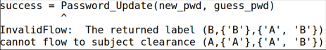
Figure 14. Pifthon throwing error

This demands a controlled downgrading. There are two possibilities for introducing downgrading at the point of returning the value: first, have an assertion that ensures downgrading explicitly, and second, perform downgrading implicitly at the function return. Pifthon follows the former approach where the expression downgrade($x$,$\{p_{1},\dots\}$) enables the programmer to specify a set of new readers. While the existing IFC literature primarily follows the downgrading mechanism of (Myers et al., [n.d.]; Stefan et al., 2011a) which is similar to discretionary, Pifthon follows the downgrading rule of RWFM where downgrading is limited to the principals who had influenced the information at some earlier stages of information flow – thus providing specific constraints:
The construct downgrade($x$,$\{p_{1}\}$) executed by $p$ adds $p_{1}$ to the readers list of label of $x$ only if:

• $p$ is the owner of the label and sole contributor of $x$ then $p$ may add any principal, e.g., $p_{1}$ into the readers set of $x$,

• $p_{1}$ is one of the sources that influenced $x$ earlier then $p_{1}$ may be added to the readers list of $x$.

As per the semantics of downgrading shown in Figure 12, downgrade($x$,$\{p_{1}\}$) executed by principal $p$ relabels variable $x$ by adding reader $p_{1}$ into the current set of readers on performing the checks described above. Downgrade mechanism above enforces a constraints on drop in confidentiality.

Thus, explicit downgrading return downgrade(result, {‘A’}) enables principal $A$ to access the outcome of the computation in password update program.

7. Pifthon Experiences

Here, we illustrate an effective use of Pifthon in the analysis of Man-in-the-Middle (MITM) attack in Diffie-Hellman (DH) cryptographic key exchange protocol (Diffie and Hellman, 1976).

Case Study: Consider two entities $A$ and $B$ generating a shared private key $K$ using DH protocol. Let $I$ be the intruder, and $S$ denote the system executing the program. A MITM attack is an outcome of two interleaving runs of DH protocol. In the first run, $I$ initiates a session with $A$ impersonating $B$. In the second run, $I$ further initiates a session with $B$ impersonating $A$. We instrument the attack in a PyX code and feed the program to Pifthon along with the static labels of the global variables and subject clearances of functions given in Table 9 . Labels comply with the security specification of the protocol. Suppose the subject executing the program has clearance label $(S,\{S\},\{A,B,S,I\})$. Then, Pifthon performs the following label computation that prevents MITM attack (for simplicity, the network has been ignored):
(1) $A$ and $B$ agree on two public prime numbers $g$ and $p$.
(2) $A$ chooses a large random number $a$ as her private key and computes $m_{a}=g^{a}\text{ mod }p$ that evaluates the label of $m_{a}$ as $(A,\{A,S\},\{A,B\})$.
(3) Since the label does not include $B$ in the readers set, we downgrade the label of $m_{a}$ from $(A,\{A,S\},\{A,B\})$ to $(A,\{A,B,S\},\{A,B\})$ before sending the message to $B$.
         (3a) $I$ chooses a random number $i$ as her private key to evaluate $m_{i}=g^{i}\text{ mod }p$, which she sends to $A$ impersonating $B$. Message $m_{i}$ obtains the label $(I,\{I,S\},\{A,B,I\})$, and further downgraded to $(I,\{I,A,S\},\{A,B,I\})$ before sending it to $A$.
(4) Similarly, $B$ chooses a number $b$ to be her private key and computes $m_{b}=g^{b}\text{ mod }p$. The label of $m_{b}$ is downgraded to $(B,\{A,B,S\},\{A,B\})$ before sending it to $A$.
         (4a) $I$ computes $m_{i}=g^{i}\text{ mod }p$ and downgrades the label of $m_{i}$ to $(I,\{I,B,S\},\{A,B,I\})$ before sending it to $B$ impersonating $A$.
(5) Next, $A$ computes shared private key $K_{AI}$ by evaluating $(g^{i})^{a}\text{ mod }p$. $K_{AI}$ obtains label $(A,\{A,S\},\{A,B,I\})$.
(6) Similarly, $B$ obtains shared private key $K_{BI}=(g^{i})^{b}\text{ mod }p$ that receives label $(B,\{B,S\},\{A,B,I\})$.

Thus, any attempt to communicate with $B$ would require $A$ to encrypt the message using $K_{AI}$ and subsequently downgrade the label of the encrypted message to $B$. Since $A$ downgrades the label only to $B$, naturally intruder $I$ would fail to access the message. Furthermore, an attempt to intercept communication by the intruder even at an early stage (3(a) or 4(a)) will fail as messages $m_{a}$ and $m_{b}$ are downgraded, particularly for $A$ and $B$ respectively.

Table 9. Given RWFM labels for Diffie-Hellman-MITM

Objects	RWFM labels
	Owner	Readers	Writers
$g$	$S$	$\{*\}$	$\{A,B\}$
$p$	$S$	$\{*\}$	$\{A,B\}$
$a$	$A$	$\{A,S\}$	$\{A\}$
$b$	$B$	$\{B,S\}$	$\{B\}$
$i$	$I$	$\{B,S\}$	$\{B\}$

Functions	RWFM labels
	Owner	Readers	Writers
creating_m_a	$A$	$\{A,S\}$	$\{A,B,S\}$
creating_k_ai	$A$	$\{A,S\}$	$\{A,B,S\}$
creating_m_b	$B$	$\{B,S\}$	$\{A,B,S\}$
creating_k_bi	$B$	$\{B,S\}$	$\{A,B,S\}$
creating_m_i	$I$	$\{I,S\}$	$\{A,B,I,S\}$

We have also used Pifthon for building a spectrum of security-critical benchmark applications with varying security properties and sizes. Table 10 lists a few well-known security applications and cryptography protocols that we have developed on our secure platform. Thus, we have tested Pifthon with the intention to identify flow-leaks (for security applications) and MITM attacks (for cryptography protocols) for a given sets of global variables and labels.

Table 10. List of application developed using Pifthon

Application Type	Applications
Security Applications	Meeting scheduling system (Roy et al., 2009)
	Conf. review system $\lambda\text{Chair}$ (Stefan et al., 2011b)
	Password update program (Myers and Askarov, 2011)
	WebTax example (Myers and Liskov, 2000)
	Vickrey auction (Chong and Myers, 2006)
Cryptography Protocols	Needham-Schroeder Public Key Protocol (Needham and Schroeder, 1978)
	Neuman-Stubblebine Protocol (ord Neuman and Stubblebine, 1993)
	Yahalom Protocol (Abadi and Tuttle, 1990)
	Wide-Mouth-Frog Protocol (Burrows et al., 1989)
	Otway-Rees Protocol (Otway and Rees, 1987)
	Diffie-Hellman Protocol (Diffie and Hellman, 1976)

Usability of Pifthon: Following features of Pifthon improve usability and meet the demands of researchers (Hicks et al., 2007, 2006; Johnson et al., 2015; Hammer, 2010):
$\bullet$ $pc$-monotonic approach enables tracking $pc$-label at any program point, including nested selection and iteration statements;
$\bullet$ It has provision to immutably label I/O channels catering to the design of distrusted communication channels;
$\bullet$ Since the labelling mechanism is compositional and preserves end-to-end non-interference – allowing data sharing between mutually distrusted distributed applications;
$\bullet$ A single input file contains the label specification for an application that eases alteration in security policies in one place and helps propagate changes throughout the program.

8. Comparison with Related Work

Here, we present a comparative study in terms of labelling approaches with prominent IFC tools and flow-security against different classes of information channels such as termination-channels.

Information Flow Control Tools:
Language-based security literature witnesses a plethora of IFC tools and platforms that have been developed in the last decade to enforce confidentiality and integrity in prevailing programming languages based on the different flow security models (Denning, 1975; Myers and Liskov, 2000; Stefan et al., 2011a). For example, security-typed languages and monitors such as Jif (Myers et al., [n.d.]), JOANA (Graf et al., 2013), Paragon (Broberg et al., 2013) for Java, FlowFox (De Groef et al., 2012), JSFlow (Hedin et al., 2014), IFC4BC (Bichhawat et al., 2014) for JavaScript, FlowCaml (Simonet and Rocquencourt, 2003) for Caml, $\lambda_{DSec}$ (Zheng and Myers, 2007) for lambda calculus, LIO (Stefan et al., 2011b), HLIO (Buiras et al., 2015), Flamio (Pedersen and Chong, 2019) for Haskell and SPARK flow analysis (Barnes, 2003) for SPARK, and flow secure platforms for instance, Jif/split (Zdancewic et al., 2002), Asbestos (Efstathopoulos et al., 2005), HiStar (Zeldovich et al., 2006), Flume (Krohn et al., 2007), Aeolus (Cheng et al., 2012) are some of the prominent ones. Table 11 shows a comparison among some of the secure languages and monitors in terms of different label binding mechanisms (cf. Section 1).

Table 11. Comparison of IFC tools and platforms

Tools	Labelling	Flow	Termination
and Platforms	mechanism	-sensitive	-sensitive
Jif	$P_{1}$	✗	✗
Paragon	$P_{1}$	✗	✗
FlowCaml	$P_{1}$	✗	✗
$\lambda_{DSec}$	$P_{3}$	✓	✗
LIO	$P_{2}$	✗	✗
$\lambda_{l,FS}^{\texttt{LIO}}$	$P_{2}+P_{4}$	✓	✗
Aeolus	$P_{1}$	✗	✗
Flamio	$P_{2}$	✗	✗
Pifthon	$P_{2}+P_{4}$	✓	✓

Comparison with IFC tools:
Jif (Myers et al., [n.d.]) is one of the prominent security typed-languages that follow a static flow analysis with $pc$-reset approach for a subset of Java. Jif follows labelling mechanism $P_{1}$ that often result in false-positives – a secure program shown in Table 3 may be identified as insecure by Jif. Further, the semantics of Jif cannot identify flow-leaks due to termination-and progress-channels.

JOANA (Graf et al., 2013) performs a compelling flow analysis for Java, based on a system dependence graph (Hammer and Snelting, 2009) that overcomes some of the shortcomings of Jif. In a dependence graph, each statement is a node, and an edge represents a dependency relation between two statements. Intuitively, a path in the graph that originates at a high node and ends at low indicates a violation of flow security. However, the flow analysis does not create any dependency between a loop and the following node unless they share an object. This limitation will not detect information leaks due to termination-channels, that makes it termination-insensitive.

Zheng et al. (Zheng and Myers, 2007) were the first to introduce a dynamic flow-sensitive analysis in their work on a security-typed $\lambda$-calculus, $\lambda_{DSec}$, that supports first-class dynamic labels that can be checked and changed at run-time. Contrary to Pifthon, $\lambda_{DSec}$ retains a static $pc$-label that acts as an upper bound of the caller. Thus, the language falls in class $P_{3}$. Moreover, the non-interference property discussed in $\lambda_{DSec}$ is termination-insensitive.

A labelled IO Haskell library LIO (Stefan et al., 2011b) shares a common paradigm but subsumes the results of $\lambda_{DSec}$. Analogous to program-counter, LIO maintains a current label that is mutable and evaluated as the upper bound of all the objects and inputs observed at run-time. While performing an output operation, LIO ensures the current label can-flow-to target object label, thus enforces flow security.

Although our work overlaps a bit with that of LIO, subtle differences are as follows: (i) compared to compile-time analysis, LIO follows a run-time floating-label approach, (ii) LIO is termination-insensitive (Stefan et al., 2012), and (iii) unlike achieving flow-senstivity for each intermediate object, LIO is flow-sensitive for the current label only, hence follows class $P_{2}$.

To overcome flow-insensitivity in LIO, an extension introduces a meta-label for each reference label (Buiras et al., 2014). Meta-label describes the confidentiality of LIO reference label. Then upgrading a reference label also considers the meta-labels besides the label on the data stored in the reference. Authors presented a precise semantics for an extension of $\lambda$-calculus called $\lambda_{l,FS}^{\texttt{LIO}}$. However, contrary to Pifthon, in the sequential context, the non-interference followed by this flow-sensitive extension of LIO is termination-insensitive.

Another Haskell library, i.e., Flamio (Pedersen and Chong, 2019), enforces coarse-grained dynamic information flow control, called FLAM (Arden et al., 2015). Flamio is a language instantiation of FLAM into LIO that can leverage it’s decentralized authorization model and distributed proof search of trust relationships. However, similar to LIO, Flamio is flow-sensitive in computation context only, hence follows class $P_{2}$, and non-interference is termination-insensitive.

Complementing recent IFC efforts that follow a run-time analysis, e.g., LIO (Stefan et al., 2011b), $\lambda_{l,FS}^{\texttt{LIO}}$ (Buiras et al., 2014), Pifthon performs a compile-time flow analysis for a dialect of Python language. The run-time analysis has the following advantages: (i) it allows running non-interfering executions selectively, providing an essence of “lazy” analysis; (ii) it enables users to perceive control dependency precisely. For instance, the analysis could accurately identify the source index of a list data structure or the source information that depends on the user inputs. Whereas, the compile-time approaches, including Pifthon, aim to capture all possible flow channels, including the non-executing control paths, thus mitigate the risk of information leaks. However, it may not accurately identify the information source that depends on the expression resolution or user inputs.

From the above comparative study, we can infer that Pifthon stands out in enabling the user to precisely determine the leaks, in the context of flow-sensitive information flow analysis that includes termination- and progress-sensitive flow channels.

9. Conclusions

In this paper, we have proposed an information flow analysis approach based on a semi-dynamic (hybrid) labelling. Using the approach, we have built Pifthon for analyzing information flow violations for a variant of Python language called PyX. The platform can be easily adapted for a variety of imperative programming languages. The security platform is quite precise as compared to various other platforms and is capable of analyzing termination-sensitive programs. We have demonstrated applications of the platform for a variety of typical security-critical programs and cryptography protocols used for security analysis. We have been using the platform for analyzing programs of reasonable size and found quite encouraging as it finds flow violations that help the user to fix the same. Our approach is proved to be sound in terms of classical non-interference freedom.

Further work is in progress to include features like exception handling, operations on mutable data structures, object creation, and initialization, etc., that invariably demand run-time analysis in Pifthon and to extend the platform for concurrent programs capable of performing IO.

Appendix A Termination of $\mathbf{Pifthon}$ Labelling Mechanism

Proposition 1.

For any given PyX program $c$ not containing iteration, and execution state $[\sigma,\lambda]$, the evaluation of $\Gamma\vdash\langle c,\sigma,\lambda\rangle$ in Pifthon always terminates.

Proof.

The proof can be shown by structural induction. The proposition holds good for the base cases pass, and $x=e$. For the inductive step, it is easy to prove that if the proposition holds for $c_{1}$ and $c_{2}$, then it also holds for conditional and sequence statements. ∎

Proposition 2.

For any given statement $c$ that does not contain nested loop, and execution context $[\sigma,\lambda]$, the evaluation $\Gamma\vdash\langle\texttt{while }e:c,\sigma,\lambda\rangle$ in Pifthon always terminates.

Proof.

From the Pifthon labelling semantics, we note that the only case in which the evaluation of $\Gamma\vdash\langle\texttt{while }e:c,\sigma,\lambda\rangle$ does not terminate is when either the evaluation of $\Gamma\vdash\langle c,\sigma,\lambda^{\prime}\rangle$ does not terminate, or $\Gamma\vdash\langle\texttt{while }e:c,\sigma,\bullet\rangle$ goes into an infinite recursion.

The former is not possible due to Proposition 1. Impossibility of the latter is shown by considering the evaluation of $\Gamma\vdash\langle\texttt{while }e:c,\sigma,\lambda\rangle$:

1. $\Gamma\vdash\langle e,\sigma,\lambda\rangle\downarrow v^{l}$, $\lambda_{1}(pc)=l\oplus\lambda(pc)$.

2. $\Gamma\vdash\langle c,\sigma,\lambda_{1}\rangle\rightarrow\langle\epsilon,\sigma_{1},\lambda_{2}\rangle$.

3. If $\lambda_{2}=\lambda_{1}$ the evaluation terminates and there is nothing to prove. So we assume that $\lambda_{2}\neq\lambda_{1}$. In this case $\Gamma\vdash\langle\texttt{while }e:c,\sigma,\lambda_{2}\rangle$ is invoked which proceeds as follows.

4. $\Gamma\vdash\langle e,\sigma_{1},\lambda_{2}\rangle\downarrow v^{l}$, $\lambda_{3}(pc)=l\oplus\lambda_{2}(pc)$.

5. $\Gamma\vdash\langle c,\sigma_{1},\lambda_{3}\rangle\rightarrow\langle\epsilon,\sigma_{1},\lambda_{4}\rangle$.

6. If $\lambda_{4}=\lambda_{3}$ the evaluation terminates and there is nothing to prove. So we assume that $\lambda_{4}\neq\lambda_{3}$. In this case $\Gamma\vdash\langle\texttt{while }e:c,\sigma,\lambda_{4}\rangle$ is invoked which proceeds as follows.

7. $\Gamma\vdash\langle e,\sigma_{1},\lambda_{4}\rangle\downarrow v^{l}$, $\lambda_{5}(pc)=l\oplus\lambda_{4}(pc)$.

8. $\Gamma\vdash\langle c,\sigma_{1},\lambda_{5}\rangle\rightarrow\langle\epsilon,\sigma_{1},\lambda_{6}\rangle$.

We claim that $\lambda_{6}=\lambda_{5}$. The proof is given below.

1. First iteration:

   $$\begin{split}l&=\lambda(pc)\oplus_{v\in var(e)\cap G}\lambda(v)\\ \lambda_{1}(pc)&=l\oplus\lambda(pc)\\ \lambda_{2}(pc)&=\lambda_{1}(pc)\oplus_{v\in SV(c)\cap G}\lambda(v)\\ &=\lambda(pc)\oplus_{v\in var(e)\cap G}\lambda(v)\oplus_{v\in SV(c)\cap G}\lambda(v)\\ &=\lambda(pc)\oplus_{v\in(var(e)\cup SV(c))\cap G}\lambda(v)\\ \end{split}$$

2. Second iteration:

   $$\begin{split}\lambda_{3}(pc)&=\lambda_{2}(pc)\oplus_{v\in var(e)\cap G}\lambda(v)\\ &=\lambda(pc)\oplus_{v\in(var(e)\cup SV(c))\cap G}\lambda(v)\\ &\oplus_{v\in var(e)\cap G}\lambda(v)\\ &=\lambda(pc)\oplus_{v\in(var(e)\cup SV(c))\cap G}\lambda(v)\\ \end{split}$$

   $$\begin{split}\lambda_{4}(pc)&=\lambda_{3}(pc)\oplus_{v\in SV(c)\cap G}\lambda(v)\\ &=\lambda(pc)\oplus_{v\in(var(e)\cup SV(c))\cap G}\lambda(v)\\ \lambda_{4}(x)&=\lambda_{3}(x)\oplus\lambda_{3}(pc)\oplus_{v\in SV(c)\cap G}\lambda(v)\\ &=\lambda_{3}(x)\oplus\lambda_{3}(pc)\\ &\text{This is because the label of $pc$ is already }\\ &\text{influenced by all the global variables in }c.\\ &=\lambda_{2}(x)\oplus\lambda(pc)\oplus_{v\in(var(e)\cup SV(c))\cap G}\lambda(v)\end{split}$$

3. Third iteration:

   $$\begin{split}\lambda_{5}(pc)&=\lambda_{4}(pc)\oplus_{v\in var(e)\cap G}\lambda(v)\\ &=\lambda(pc)\oplus_{v\in(var(e)\cup SV(c))\cap G}\oplus_{v\in var(e)\cap G}\lambda(v)\\ &=\lambda(pc)\oplus_{v\in(var(e)\cup SV(c))\cap G}\lambda(v)\\ \lambda_{5}(x)&=\lambda_{4}(x)\\ &=\lambda_{2}(x)\oplus\lambda(pc)\oplus_{v\in(var(e)\cup SV(c))\cap G}\lambda(v)\end{split}$$

   $$\begin{split}\lambda_{6}(pc)&=\lambda_{5}(pc)\oplus_{v\in SV(c)\cap G}\lambda(v)\\ &=\lambda(pc)\oplus_{v\in(var(e)\cup SV(c))\cap G}\lambda(v)\\ \lambda_{6}(x)&=\lambda_{5}(x)\oplus\lambda_{5}(pc)\oplus_{v\in SV(c)\cap G}\lambda(v)\\ &=\lambda_{2}(x)\oplus\lambda(pc)\oplus_{v\in(var(e)\cup SV(c))\cap G}\lambda(v)\end{split}$$

It can be observed that $\lambda_{6}=\lambda_{5}$. Thus, we can conclude that for the iteration statement, Pifthon labelling procedure terminates after a maximum of three iterations. ∎

Appendix B Labelling the Password Update Program

Pifthon performs the following operations as shown in Table 12. At line 3, $pc$ label become equal to LUB of the labels of $pwd\_db$ and $guess\_pwd$. Next it checks the constraint for allowing the implicit flow from if-guard to the target variable $pwd\_db$. At line 4, as target $pwd\_db$ is a global variable, therefore, Pifthon checks if the condition $\lambda(pc)\oplus\lambda(new\_pwd)\oplus cl\leqslant\lambda(pwd\_db)$ holds true. Finally, at line 5, label of local variable $result$ is updated by the $pc$ label, thus obtain the final label of $result$.

Table 12. Steps performed by Pifthon for computing final label of $result$

Line No.	Label Computations & Constraints
2	Initial label of $pc$ is $\lambda(pc)=$ (B,{*},{ })
3	(i) $l=\lambda(pwd\_db)\oplus\lambda(guess\_pwd)=$(B,{B},{A,B})
	(ii) $\lambda(pc)=l\oplus\lambda(pc)=$(B,{B},{A,B})
	(iii) $\lambda(pc)\leqslant\lambda(pwd\_db)$
4	(i) $\lambda(pc)=\lambda(new\_pwd)\oplus\lambda(pc)=$ (B,{B},{A,B});
	(ii) $\lambda(pc)\oplus cl\leqslant\lambda(pwd\_db)$
5	$\lambda(result)=\lambda(pc)=$(B,{B},{A,B})

Appendix C Output of $\mathbf{Pifthon}$ For Programs

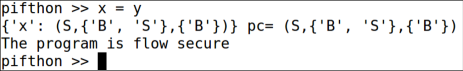
Figure 15. Output of an assignment $x=y$, where $x$ is a local variable, $\lambda(y)=(B,\{B,S\},\{B\})$, and $cl=(S,\{S\},\{A,B\})$ (Cf. Table 6)

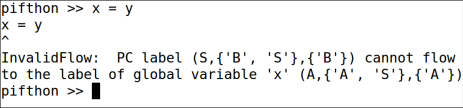
Figure 16. Output of an assignment $x=y$, where $x$ is a global variable, $\lambda(x)=(A,\{A,S\},\{A\})$ $\lambda(y)=(B,\{B,S\},\{B\})$, and $cl=(S,\{S\},\{A,B\})$ (Cf. Table 6)

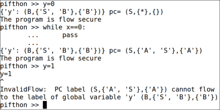
Figure 17. Pifthon throws error for a termination-sensitive information leak (Cf. Figure 7)

References

- (1)
- Abadi et al. (1999) Martín Abadi, Anindya Banerjee, Nevin Heintze, and Jon G Riecke. 1999. A core calculus of dependency. In Proceedings of the 26th ACM SIGPLAN-SIGACT symposium on Principles of programming languages. ACM, 147–160.
- Abadi and Tuttle (1990) Martin Abadi and Mark R Tuttle. 1990. A logic of authentication. In ACM Transactions on Computer Systems. Citeseer.
- Arden et al. (2015) Owen Arden, Jed Liu, and Andrew C Myers. 2015. Flow-limited authorization. In 2015 IEEE 28th Computer Security Foundations Symposium. IEEE, 569–583.
- Askarov et al. (2008) Aslan Askarov, Sebastian Hunt, Andrei Sabelfeld, and David Sands. 2008. Termination-insensitive noninterference leaks more than just a bit. In European symposium on research in computer security. Springer, 333–348.
- Askarov and Sabelfeld (2009) Aslan Askarov and Andrei Sabelfeld. 2009. Tight enforcement of information-release policies for dynamic languages. In Proc. of 22nd CSF Symposium. 43–59.
- Austin and Flanagan (2009) Thomas H Austin and Cormac Flanagan. 2009. Efficient purely-dynamic information flow analysis. In Proc. of the 4th Workshop on PLAS. 113–124.
- Banerjee and Naumann (2002) Anindya Banerjee and David A Naumann. 2002. Secure Information Flow and Pointer Confinement in a Java-like Language.. In CSFW, Vol. 2. 253.
- Barnes (2003) John Gilbert Presslie Barnes. 2003. High integrity software: the spark approach to safety and security. Pearson Education.
- Bichhawat et al. (2014) Abhishek Bichhawat, Vineet Rajani, Deepak Garg, and Christian Hammer. 2014. Information flow control in WebKit’s JavaScript bytecode. In Proc. of Int. Conf. on Principles of Security and Trust. Springer, 159–178.
- Broberg et al. (2013) Niklas Broberg, Bart van Delft, and David Sands. 2013. Paragon for practical programming with information-flow control. In APLAS. Springer, 217–232.
- Buiras et al. (2014) Pablo Buiras, Deian Stefan, and Alejandro Russo. 2014. On dynamic flow-sensitive floating-label systems. In Proc. of IEEE 27th CSF Symposium. 65–79.
- Buiras et al. (2015) Pablo Buiras, Dimitrios Vytiniotis, and Alejandro Russo. 2015. HLIO: Mixing static and dynamic typing for information-flow control in Haskell. In ACM SIGPLAN Notices, Vol. 50. ACM, 289–301.
- Burrows et al. (1989) Michael Burrows, Martin Abadi, and Roger Michael Needham. 1989. A logic of authentication. Proceedings of the Royal Society of London. A. Mathematical and Physical Sciences 426, 1871 (1989), 233–271.
- Cheng et al. (2012) Winnie Cheng, Dan RK Ports, David A Schultz, Victoria Popic, Aaron Blankstein, James A Cowling, Dorothy Curtis, Liuba Shrira, and Barbara Liskov. 2012. Abstractions for Usable Information Flow Control in Aeolus.. In USENIX Annual Technical Conference. 139–151.
- Chong and Myers (2006) Stephen Chong and Andrew C Myers. 2006. Decentralized robustness. In Computer Security Foundations Workshop, 19th IEEE. 12–pp.
- De Groef et al. (2012) Willem De Groef, Dominique Devriese, Nick Nikiforakis, and Frank Piessens. 2012. FlowFox: a web browser with flexible and precise information flow control. In Proc. of ACM CCS. 748–759.
- Denning (1976) Dorothy E Denning. 1976. A lattice model of secure information flow. CACM 19, 5 (1976), 236–243.
- Denning and Denning (1977) Dorothy E Denning and Peter J Denning. 1977. Certification of programs for secure information flow. Commun. ACM 20, 7 (1977), 504–513.
- Denning (1975) Dorothy Elizabeth Robling Denning. 1975. Secure information flow in computer systems. (1975).
- Diffie and Hellman (1976) Whitfield Diffie and Martin Hellman. 1976. New directions in cryptography. IEEE transactions on Information Theory 22, 6 (1976), 644–654.
- Efstathopoulos et al. (2005) Petros Efstathopoulos, Maxwell Krohn, Steve VanDeBogart, Cliff Frey, David Ziegler, Eddie Kohler, David Mazieres, Frans Kaashoek, and Robert Morris. 2005. Labels and event processes in the Asbestos operating system. In Proc. of 20th ACM SOSP, Vol. 39. 17–30.
- Goguen and Meseguer (1982) Joseph A Goguen and José Meseguer. 1982. Security policies and security models. In IEEE Symposium on SP. 11–11.
- Graf et al. (2013) Jürgen Graf, Martin Hecker, and Martin Mohr. 2013. Using JOANA for Information Flow Control in Java Programs - A Practical Guide. In Proceedings of the 6th Working Conference on Programming Languages (ATPS’13) (Lecture Notes in Informatics (LNI) 215). Springer Berlin / Heidelberg, 123–138.
- Hammer (2010) Christian Hammer. 2010. Experiences with PDG-based IFC. In International Symposium on Engineering Secure Software and Systems. Springer, 44–60.
- Hammer and Snelting (2009) Christian Hammer and Gregor Snelting. 2009. Flow-sensitive, context-sensitive, and object-sensitive information flow control based on program dependence graphs. Int. Journal of Information Security 8, 6 (2009), 399–422.
- Hedin et al. (2014) Daniel Hedin, Arnar Birgisson, Luciano Bello, and Andrei Sabelfeld. 2014. JSFlow: Tracking information flow in JavaScript and its APIs. In Proc. of 29th Annual ACM SAC. 1663–1671.
- Hedin and Sabelfeld (2012) Daniel Hedin and Andrei Sabelfeld. 2012. A Perspective on Information-Flow Control. In Software Safety and Security - Tools for Analysis and Verification. 319–347.
- Hicks et al. (2006) Boniface Hicks, Kiyan Ahmadizadeh, and Patrick McDaniel. 2006. From languages to systems: Understanding practical application development in security-typed languages. In 2006 22nd ACSAC. IEEE, 153–164.
- Hicks et al. (2007) Boniface Hicks, Dave King, and Patrick McDaniel. 2007. Jifclipse: development tools for security-typed languages. In Proc. of Workshop on PLAS. 1–10.
- Honda and Yoshida (2002) Kohei Honda and Nobuko Yoshida. 2002. A uniform type structure for secure information flow. Vol. 37. ACM.
- Hunt and Sands (2006) Sebastian Hunt and David Sands. 2006. On flow-sensitive security types. In ACM SIGPLAN Notices, Vol. 41. 79–90.
- Johnson et al. (2015) Andrew Johnson, Lucas Waye, Scott Moore, and Stephen Chong. 2015. Exploring and enforcing security guarantees via program dependence graphs. In ACM SIGPLAN Notices, Vol. 50. ACM, 291–302.
- King et al. (2007) Dave King, Susmit Jha, Trent Jaeger, Somesh Jha, and Sanjit A Seshia. 2007. On Automatic Placement of Declassifiers for Information-Flow Security. Technical Report. Technical Report NASTR-0083-2007.
- Krohn et al. (2007) Maxwell N. Krohn, Alexander Yip, Micah Z. Brodsky, Natan Cliffer, M. Frans Kaashoek, Eddie Kohler, and Robert Morris. 2007. Information flow control for standard OS abstractions. In Proc. of 21st ACM SOSP. 321–334.
- Kumar and Shyamasundar (2017) N. V. Narendra Kumar and R.K. Shyamasundar. 2017. A Complete Generative Label Model for Lattice-Based Access Control Models. In International Conference on Software Engineering and Formal Methods. Springer, 35–53.
- Kumar and Shyamasundar (2014) N. V. Narendra Kumar and R. K. Shyamasundar. 2014. Realizing purpose-based privacy policies succinctly via information-flow labels. In Big Data and Cloud Computing (BdCloud), IEEE 4th. Int. Conf. on. 753–760.
- Le Guernic (2007) Gurvan Le Guernic. 2007. Automaton-based confidentiality monitoring of concurrent programs. In Proc. of 20th IEEE CSF Symposium. 218–232.
- Myers and Askarov (2011) Andrew Myers and Aslan Askarov. 2011. Attacker Control and Impact for Confidentiality and Integrity. Logical Methods in Computer Science 7 (2011).
- Myers and Liskov (2000) Andrew C Myers and Barbara Liskov. 2000. Protecting privacy using the decentralized label model. ACM TOSEM 9, 4 (2000), 410–442.
- Myers et al. ([n.d.]) Andrew C Myers, Lantian Zheng, Steve Zdancewic, Stephen Chong, and Nathaniel Nystrom. [n.d.]. Jif:. http://www.cs.cornell.edu/jif ([n. d.]).
- Needham and Schroeder (1978) Roger M Needham and Michael D Schroeder. 1978. Using encryption for authentication in large networks of computers. Commun. ACM 21, 12 (1978), 993–999.
- ord Neuman and Stubblebine (1993) B Cli ord Neuman and Stuart G Stubblebine. 1993. A note on the use of timestamps as nonces. Operating Systems Review 27, 2 (1993), 10–14.
- Otway and Rees (1987) Dave Otway and Owen Rees. 1987. Efficient and timely mutual authentication. ACM SIGOPS Operating Systems Review 21, 1 (1987), 8–10.
- Pedersen and Chong (2019) Mathias Vorreiter Pedersen and Stephen Chong. 2019. Programming with Flow-Limited Authorization: Coarser is Better. In 2019 IEEE EuroS&P. IEEE, 63–78.
- Pottier and Simonet (2002) François Pottier and Vincent Simonet. 2002. Information flow inference for ML. In ACM SIGPLAN Notices, Vol. 37. ACM, 319–330.
- Robling Denning (1982) Dorothy Elizabeth Robling Denning. 1982. Cryptography and data security. Addison-Wesley Longman Publishing Co.
- Roy et al. (2009) Indrajit Roy, Donald E. Porter, Michael D. Bond, Kathryn S. McKinley, and Emmett Witchel. 2009. Laminar: practical fine-grained decentralized information flow control. In Proceedings of ACM SIGPLAN PLDI. 63–74.
- Russo and Sabelfeld (2010) Alejandro Russo and Andrei Sabelfeld. 2010. Dynamic vs. static flow-sensitive security analysis. In 2010 23rd IEEE CSF Symposium. 186–199.
- Sabelfeld and Myers (2003) Andrei Sabelfeld and Andrew C Myers. 2003. A model for delimited information release. In International Symposium on Software Security. Springer, 174–191.
- Simonet and Rocquencourt (2003) Vincent Simonet and Inria Rocquencourt. 2003. Flow Caml in a nutshell. In Proc. of 1st APPSEM-II workshop. 152–165.
- Smith et al. (2001) Geoffrey Smith et al. 2001. A New Type System for Secure Information Flow.. In CSFW, Vol. 1. 4.
- Stefan et al. (2012) Deian Stefan, Alejandro Russo, Pablo Buiras, Amit Levy, John C Mitchell, and David Maziéres. 2012. Addressing covert termination and timing channels in concurrent information flow systems. In ACM SIGPLAN Notices, Vol. 47. 201–214.
- Stefan et al. (2011a) Deian Stefan, Alejandro Russo, David Mazières, and John C Mitchell. 2011a. Disjunction category labels. In Nordic conference on secure IT systems. Springer, 223–239.
- Stefan et al. (2011b) Deian Stefan, Alejandro Russo, John C Mitchell, and David Mazières. 2011b. Flexible dynamic information flow control in Haskell. In Proc Haskell. 95–106.
- Volpano and Smith (1997) Dennis Volpano and Geoffrey Smith. 1997. Eliminating covert flows with minimum typings. In Proceedings 10th CSFW. IEEE, 156–168.
- Volpano et al. (1996) Dennis M. Volpano, Cynthia E. Irvine, and Geoffrey Smith. 1996. A Sound Type System for Secure Flow Analysis. Journal of Computer Security 4, 2/3 (1996), 167–188. https://doi.org/10.3233/JCS-1996-42-304
- Zdancewic and Myers (2001) Steve Zdancewic and Andrew C Myers. 2001. Robust Declassification.. In CSFW, Vol. 1. 15–23.
- Zdancewic and Myers (2002) Steve Zdancewic and Andrew C Myers. 2002. Secure information flow via linear continuations. Higher-Order and Symbolic Computation 15, 2-3 (2002), 209–234.
- Zdancewic et al. (2002) Steve Zdancewic, Lantian Zheng, Nathaniel Nystrom, and Andrew C Myers. 2002. Secure program partitioning. ACM TOCS 20, 3 (2002), 283–328.
- Zeldovich et al. (2006) Nickolai Zeldovich, Silas Boyd-Wickizer, Eddie Kohler, and David Mazières. 2006. Making Information Flow Explicit in HiStar. In Proc. of 7th Symp. on OSDI. 263–278.
- Zheng and Myers (2007) Lantian Zheng and Andrew C Myers. 2007. Dynamic security labels and static information flow control. International Journal of Information Security 6, 2-3 (2007), 67–84.