Event-Triggered Distributed Estimation With Decaying Communication Rate

Abstract

We study distributed estimation of a high-dimensional static parameter vector through a group of sensors whose communication network is modeled by a fixed directed graph. Different from existing time-triggered communication schemes, an event-triggered asynchronous scheme is investigated in order to reduce communication while preserving estimation convergence. A distributed estimation algorithm with a single step size is first proposed based on an event-triggered communication scheme with a time-dependent decaying threshold. With the event-triggered scheme, each sensor sends its estimate to neighbor sensors only when the difference between the current estimate and the last sent-out estimate is larger than the triggering threshold. Different sensors can have different step sizes and triggering thresholds, enabling the parameter estimation process to be conducted in a fully distributed way. We prove that the proposed algorithm has mean-square and almost-sure convergence respectively, under an integrated condition of sensor network topology and sensor measurement matrices. The condition is satisfied if the topology is a balanced digraph containing a spanning tree and the system is collectively observable. The collective observability is the possibly mildest condition, since it is a spatially and temporally collective condition of all sensors and allows sensor measurement matrices to be time-varying, stochastic, and non-stationary. Moreover, we provide estimates for the convergence rates, which are related to the step size as well as the triggering threshold. Furthermore, as an essential metric of sensor communication intensity in the event-triggered distributed algorithms, the communication rate is proved to decay to zero with a certain speed almost surely as time goes to infinity. In addition, we show that it is feasible to tune the threshold and the step size such that requirements of algorithm convergence and communication rate decay are satisfied simultaneously. We also show that given the step size, adjusting the decay speed of the triggering threshold can lead to a tradeoff between the convergence rate of the estimation error and the decay speed of the communication rate. Specifically, increasing the decay speed of the threshold would make the communication rate decay faster, but reduce the convergence rate of the estimation error. Numerical simulations are provided to illustrate the developed results.

1 Introduction

Networked systems monitoring complex environments generate a tremendous amount of data, which can be used in the estimation of system states or unknown parameters. Parameter estimation is one of the most important tools in control theory, signal processing, and machine learning with extensive applications in sensor networks, weather prediction, cyber-physical systems, environmental monitoring, transportation, etc. The development of computational and energy efficient algorithms, which are able to handle imperfect data from sensor networks, is drawing more and more attention.

1-A Motivation and Challenges

To estimate a high-dimensional parameter vector (such as temperature over a large environment) is usually infeasible by a local algorithm for each sensor only with local measurements. Thus, it is necessary to design a collaborative estimation algorithm for sensors to obtain accurate estimates of the parameter. Centralized and distributed architectures are the two dominating approaches to sensor network estimation. In the centralized architecture, a data center runs estimation algorithms based on all sensor data in order to estimate a state or system parameter. In this way, optimality in certain sense can be ensured, such as the Kalman filter achieving the minimum variance unbiased estimate for linear dynamical systems under Gaussian noise. However, with large-scale deployment of sensors, the centralized architecture is no longer efficient. Therefore, we need to develop effective and efficient distributed estimation algorithms based on local sensor data and local sensor communication.

In distributed parameter estimation, messages shared between sensors play important roles. Since sensor measurements only contain partial parameter information, it is not sufficient to design a global parameter estimation algorithm only by communicating sensor measurements. Quite a few distributed estimators are proposed by requiring that sensors send their estimates to neighbor sensors at every time instant of measurement sampling. Diffusion-based distributed estimators are proposed in [1] and [2] by solving least-squares and least-mean-squares problems over networks. In [3], a distributed estimator based on sensor beliefs is proposed over a strongly connected communication network. In [4], a gossip distributed estimator is proposed to handle random failures of network links. The results are extended in [5] to nonlinear systems under imperfect communication channels, and extended to more general system models and communication networks in [6], where an adaptive learning method is proposed in order to achieve asymptotic efficiency. A robust distributed parameter estimator is given in [7] for systems with Markovian switching networks and uncertain measurement models. However, since the above references require that each sensor communicates with its neighbors persistently, there will be severe energy consumption and serious channel congestion if the measurement sampling rate is high or the parameter is high-dimensional. Under constrained communication resources, although the above algorithms can still work by requiring that sensors communicate periodically, their estimation performance could be much degraded.

Therefore, it is vital to develop a performance-guaranteed distributed estimation algorithm based on an effective and efficient sensor communication mechanism. Nevertheless, there are two challenges. First, for potentially time-varying, stochastic, and non-stationary sensor measurement models with weak observability (e.g., collective observability), how to guarantee the performance of the distributed algorithm under limited communications is challenging. Second, under the influence of noisy measurements, how to quantify the communication frequency of sensors is difficult.

1-B Related Work

To mitigate the issue of sensor communications, there are some approaches, including data quantization, compressed sensing, adaptive sampling, and event-triggered communications. In the following discussion, we focus our attention on adaptive sampling and event-triggered communications, since they can make better use of posterior information compared to the former two approaches.

In parameter estimation under constraint on the total sensing effort, adaptive sampling helps improve performance by strategically allocating sensing effort in future data collection based on the information extracted from data collected previously. In [8], a sequential adaptive sampling-and-refinement procedure called distilled sensing is proposed to detect and estimate parameters. The reference [9] investigates how to estimate the support set of a sparse parameter by making full use of structural information. For a class of physical-constrained sensing models, the limitations and advantages of adaptive sampling are analyzed in [10], and it is shown that a constrained adaptive sampling method can substantially improve estimation performance. Moreover, the adaptive sampling problem for a class of continuous-time Markov state processes is studied in [11]. The above and related literature require either structural information or prior distribution of parameters, which is difficult to satisfy in monitoring complex environments. In addition, many methods in the literature are introduced in the centralized architecture. It is difficult to extend these methods to the distributed architecture with large-scale sensor networks and high-dimensional system parameters.

In contrast, an event-triggered scheme is suitable to the distributed architecture under constrained communication resource, since it can efficiently determine when a sensor should share data to other sensors without the prior knowledge of parameter structure. In such a way, event-triggered sensor communications are usually asynchronous and aperiodic, thus different from traditional time-triggered communications. A number of centralized estimators with event-triggered measurement schedulers are proposed in the literature, such as [12, 13] for state estimation of dynamical systems, and [14, 15, 16] for static parameter estimation. Regarding the event-triggered parameter estimation, the authors in [14] propose a measurement scheduler such that the asymptotic estimation performance is optimized. A stochastic measurement scheduler is studied in [15] to compensate for the loss of the Gaussianity of the system, which ensures the maximum-likelihood parameter estimator. An event-triggered scheduler for finite impulse response systems with binary measurements is proposed in [16] where communication rate is analyzed. The above centralized event-triggered measurement schedulers are usually not suitable to the distributed architecture, because scheduling local measurements between neighboring sensors is insufficient to design a global parameter estimator when each sensor can only observe partial elements of the parameter vector. In the distributed architecture for event-triggered estimation, there are several methods for dynamical systems. For example, an LMI approach is studied in [17] for the cooperative estimation and control of a dynamical system under an event-triggered communication protocol. An event-triggered distributed Kalman filter is proposed in [18] and proved to be stable in terms of means-square boundedness of the estimation error in each sensor. For linear dynamical systems under state equality constraints, an event-triggered projected distributed Kalman filter is studied in [19] with guaranteed estimation error stability under collective system observability. For more related works of event-triggered distributed estimation for dynamical systems, we refer the readers to [20] and the references therein. Another related topic is event-triggered distributed optimization, which concerns the distributed design of optimization algorithms such that the global optimal solution is reached by each computational node. In this direction, most algorithms are proposed in noise-free or disturbance-free settings and analyzed to show the influence of event-triggered mechanisms on algorithm convergence [21, 22]. An event-triggered property for continuous-time systems, which is called Zeno behavior (i.e., an infinite number of events occur in a finite amount of time), is also of interest in some papers [23]. However, there are few event-triggered distributed optimization or estimation algorithms handling imperfect data from stochastic environments. In addition, the above studies analyze the influence of event-triggered threshold to estimation performance, but the tradeoff between communication frequency and estimation performance is not well established in the distributed architecture. To the best of our knowledge, there is no result of distributed parameter estimation on communication rate, which is an essential metric of sensor network communication level.

1-C Contributions

In this paper, we study the event-triggered distributed parameter estimation problem for the sake of reducing sensor communication while preserving convergence of estimators. The main contributions are summarized in the following:

1. We propose a recursive event-triggered distributed parameter algorithm with a single step size (Algorithm 1) for a group of sensors with noisy measurements. The algorithm has several advantages: First, it is fully distributed in the sense that each sensor only relies on the local information and has its own step size and triggering threshold. Second, without requiring exact noise distribution or statistics, the event-triggered scheme enables sensors to communicate in an efficient way that each sensor sends its estimate to neighboring sensors only when the difference between the current estimate and the last sent-out estimate is larger than the triggering threshold. Third, the algorithm is scalable to large-scale sensor networks, since its update is independent of the network size.

2. We prove that the proposed algorithm with a properly designed step size and triggering threshold achieves mean-square convergence (Theorem 3.1). In addition, we provide the estimate for the convergence rate and establish its connection to network structure and system observability. The results are obtained under an integrated condition of sensor network topology and sensor measurement matrices. The condition is satisfied if the topology is a balanced digraph containing a spanning tree and the system is collectively observable. The collective observability is the possibly mildest condition, since it allows each sensor to observe partial elements of the parameter, sensor measurement matrices to be time-varying, stochastic, and non-stationary, as well as the noise processes to be martingale difference sequences. Under some extra conditions on step size and triggering threshold, we prove the algorithm’s output is asymptotically convergent to the true parameter almost surely (a.s.) with an estimated convergence rate (Theorem 3.2).

3. We prove that the communication rate is decaying to zero almost surely as time goes to infinity (Theorem 3.3) with a quantified speed. Moreover, we show that it is feasible to tune the threshold and the step size such that the requirements of the algorithm convergence and the communication rate decay are satisfied simultaneously. We also show that given the step size, adjusting the decay speed of the triggering threshold can lead to a tradeoff between the convergence rate of the estimation error and the decay speed of the communication rate. Specifically, increasing the decay speed of the threshold would make the communication rate decay faster, but reduce the convergence rate of the estimation error. To the best of our knowledge, this is the first result on communication rate in the direction of event-triggered distributed algorithms for estimating static parameters or solutions [21, 23]. Our result indicates that while ensuring successful parameter estimation, the algorithm enables to alleviate channel burden and resource consumption in sensor communication compared to existing time-triggered approaches [3, 4, 6, 2, 7, 24, 25] which require a persistent positive communication rate.

The results of this paper are significantly different from the literature. Regarding the step size, we remove the requirement that all sensors share the same setting [4, 6, 5, 24, 7, 26, 25, 27], as well as the requirements of the concrete forms [4, 6, 5, 26, 25, 27] and the monotonicity in [24]. The stationarity condition of measurement matrices in [7] is removed. Since sensor measurements and measurement matrices are not shared between neighbors, our algorithm can be more suitable to the scenarios with privacy requirement than the diffusion estimators in [1, 28]. Moreover, we generalize sensor communication topologies from undirected graphs [4, 6, 5, 27] to a class of directed graphs, such as balanced digraphs containing a spanning tree.

1-D Paper Organization

In Section 2, we formulate the considered problem of event-triggered distributed parameter estimation and introduce some graph preliminaries, the communication model, and the mathematical model of sensors. In order to solve this problem, in Section 3 an event-triggered distributed estimation algorithm is proposed and analyzed in terms of estimation error convergence (mean-square and almost-sure convergence) and communication rate. For reading convenience, the proofs for the results in Section 3 are provided in Section 4. Numerical simulations in two examples are provided in Section 5 to illustrate the developed results. Section 6 concludes the paper.

Notations. Denote $\mathbb{R}^{n\times m}$ the set of real-valued matrices with $n$ rows and $m$ columns, with $\mathbb{R}^{n}=\mathbb{R}^{n\times 1}$ and $\mathbb{R}^{1}=\mathbb{R}$. Let $\mathbb{R}^{+}$ and $\mathbb{N}^{+}$ be the sets of positive real-valued scalars and integers, respectively, with $\mathbb{N}=\mathbb{N}^{+}\cup\{0\}$. Denote $\Omega$ and $\emptyset$ the universal set and empty set, respectively. $I_{n}$ stands for the $n$-dimensional square identity matrix. $\textbf{1}_{n}$ stands for the $n$-dimensional vector with all elements being one. The superscript “$\sf T$” represents the transpose. $\operatorname{\mathbb{E}}\{x\}$ denotes the mathematical expectation of the random variable $x$, and $\operatorname{blockdiag}\{\cdot\}$ represents the diagonalizations of block elements. $A\otimes B$ is the Kronecker product of $A$ and $B$. $\left\lVert x\right\rVert$ is the 2-norm of a vector $x$, and $\left\lVert A\right\rVert$ is the induced norm, i.e., $\left\lVert A\right\rVert=\sup_{\left\lVert x\right\rVert=1}\left\lVert Ax\right\rVert$, where $A\in\mathbb{R}^{n\times m}$, $x\in\mathbb{R}^{m}$. The mentioned scalars, vectors and matrices of this paper are all real-valued. Let $\sigma(\cdot)$ be the $\sigma$-algebra operator which generates the smallest $\sigma$-algebra. For a real-valued matrix or vector sequence $\{a(t)\}$ and a real number sequence $\{b(t)\}$, the operator $a(t)=O(b(t))$ means that there is a constant $c\geq 0$, such that for each element sequence of $\{a_{i}(t)\}$, $\lim\limits_{t\rightarrow\infty}|a_{i}(t)/b(t)|\leq c$, and the operator $a(t)=o(b(t))$ means $\lim\limits_{t\rightarrow\infty}|a_{i}(t)/b(t)|=0$.

2 Preliminaries and Problem Formulation

In this section, we formulate the problem of event-triggered distributed parameter estimation and introduce some graph preliminaries, the communication model, and the mathematical model of sensors.

2-A Graph Preliminaries

In this paper, the communication between $N$ sensors of a network is modeled as a digraph $\mathcal{G=(V,E,A)}$, where $\mathcal{V}=\{1,2,\dots,N\}$ is the node set, $\mathcal{E}\subseteq\mathcal{V}\times\mathcal{V}$ is the edge set. A directed edge $(i,j)\in\mathcal{E}$, if and only if there is a communication link from $j$ to $i$, where $j$ is called the parent node and $i$ is called the child node. The matrix $\mathcal{A}=[a_{i,j}]_{i,j=1}^{N}$ is the weighted adjacency matrix with $a_{i,j}\geq 0$, where $a_{i,j}>0$, if $(i,j)\in\mathcal{E}$. The parent neighbor set and child neighbor set of node $i$ are denoted by $\{j\in\mathcal{V}|(i,j)\in\mathcal{E}\}\triangleq\mathcal{N}_{i}$ and $\{j\in\mathcal{V}|(j,i)\in\mathcal{E}\}\triangleq\mathcal{N}_{i}^{c}$, respectively. Suppose that the graph has no self loop, which means $a_{i,i}=0$ for any $i\in\mathcal{V}$. $\mathcal{G}$ is called a balanced digraph, if $\sum_{j=1}^{N}a_{i,j}=\sum_{i=1}^{N}a_{j,i}$ for all $i\in\mathcal{V}$. $\mathcal{G}$ is called an undirected graph, if $\mathcal{A}$ is symmetric. The Laplacian matrix of $\mathcal{G}$ is denoted by $\mathcal{L}=\mathcal{D}-\mathcal{A}$, where $\mathcal{D}=\operatorname{diag}\{\sum_{j=1}^{N}a_{1,j},\dots,\sum_{j=1}^{N}a_{N,j}\}$. The mirror graph of the digraph $\mathcal{G}$ is an undirected graph, denoted by $\bar{\mathcal{G}}=\mathcal{(V,E_{\bar{\mathcal{G}}},A_{\bar{\mathcal{G}}})}$ with $\mathcal{A}_{\bar{\mathcal{G}}}=[\bar{a}_{i,j}]_{i,j=1}^{N}$, $\bar{a}_{i,j}=\bar{a}_{j,i}=(a_{i,j}+a_{j,i})/2$ ([29]). $\mathcal{G}$ is called strongly connected if for any pair nodes $(i_{1},i_{l})$, $l>1,$ there exists a path from $i_{l}$ to $i_{1}$ consisting of edges in the set $\{(i_{m},i_{m+1})\in\mathcal{E}|m=1,2,\dots,l-1\}$. We call $\mathcal{G}$ is connected if it is strongly connected and undirected. A directed tree is a digraph, where each node except the root has exactly one parent node. A spanning tree of $\mathcal{G}$ is a directed tree whose node set is $\mathcal{V}$ and whose edge set is a subset of $\mathcal{E}$.

2-B Problem Setup

Consider an unknown high-dimensional parameter vector $\theta\in\mathbb{R}^{M}$ observed by $N>0$ sensors with the following model

$$y_{i}(t)=H_{i}(t)\theta+v_{i}(t),i=1,2,\dots,N,$$ (1)

where $y_{i}(t)\in\mathbb{R}^{m_{i}}$ is the measurement vector, $v_{i}(t)\in\mathbb{R}^{m_{i}}$ is the measurement noise, and $H_{i}(t)\in\mathbb{R}^{m_{i}\times M}$ represents the known measurement matrix of sensor $i$, all at time $t$.

The communication rate is an essential metric of communication intensity in the event-triggered distributed algorithms. Its mathematical definition over the digraph $\mathcal{G}$ is in the following.

Definition 2.1.

For the digraph $\mathcal{G}$, in a given time interval $[0,t]\cap\mathbb{N}$, the communication rate $\lambda_{c}(t)$ is given by

$$\lambda_{c}(t)=\frac{\sum_{i\in\mathcal{V}}K_{i}(t)|\mathcal{N}_{i}^{c}|}{t\sum_{i\in\mathcal{V}}|\mathcal{N}_{i}^{c}|},$$ (2)

where $K_{i}(t)$ is the accumulated triggering (data-sending) times of node $i$ in $[0,t]\cap\mathbb{N}$, and $|\mathcal{N}_{i}^{c}|$ is the child neighbor number of node $i$.

According to this definition, $\lambda_{c}(t)\in[0,1]$. When $\lambda_{c}(t)\equiv 1$, communication occurs all the time, which is the case for the time-triggered distributed estimation algorithms [3, 4, 6, 2, 7, 24]. When $\lambda_{c}(t)\equiv 0$, there is no sensor communication over the network.

The problem considered in this paper is how to design a distributed estimation algorithm with an event-triggered communication scheme, and find conditions such that the output of the algorithm is asymptotically convergent to the parameter vector at a certain rate while the communication rate of the sensor network is decaying to zero as time goes to infinity.

3 Main results

The formulated problem is solved in this section. First, an event-triggered distributed algorithm is proposed to estimate the parameter. Then, the mean-square and almost-sure convergence of the algorithm are studied, respectively. Additionally, the decay speed of the communication rate is analyzed. The proofs of these results are provided in Section 4.

3-A Event-triggered distributed estimation

To solve the problem posed in Section 2, we propose the event-triggered distributed estimation algorithm in Algorithm 1 for each sensor $i\in\mathcal{V}$, where the initial estimate $x_{i}(0)=x_{i,0}\in\mathbb{R}^{M}$ is fixed. An example of Algorithm 1 for a sensor network with 7 nodes is provided in FIG. 1.

Algorithm 1 Event-Triggered Distributed Estimation

1:  Input: $x_{i}(0),\{y_{i}(t)\}_{t\geq 0},\{H_{i}(t)\}_{t\geq 0},\{\alpha_{i}(t)\}_{t\geq 0},\{f_{i}(t)\}_{t\geq 0}$

2:  Output: $\{x_{i}(t)\}_{t\geq 0}$

3:  for $t=0,1,\dots$ do

4:     // Data transmission

5:     if $t=0$ then

6:        Send $x_{i}(0)$ to each child neighbor sensor $j\in\mathcal{N}_{i}^{c}$ and let $x_{i}(\tau_{0})=x_{i}(0)$ and $k_{i}(0)=1$.

7:     else if $\|x_{i}(t)-x_{i}(\tau_{k_{i}(t-1)})\|>f_{i}(t)$ then

8:        Send $x_{i}(t)$ to each child neighbor sensor $j\in\mathcal{N}_{i}^{c}$ and let $k_{i}(t)=k_{i}(t-1)+1$ and $\tau_{k_{i}(t)}:=t$.

9:     else

10:        $k_{i}(t)=k_{i}(t-1)$.

11:     end if

12:     // Data receiving

13:     for $j\in\mathcal{N}_{i}$ do

14:        if Receive estimate $x_{j}(t)$ from parent neighbor sensor $j\in\mathcal{N}_{i}$ then

15:           Let $k_{j}(t)=k_{j}(t-1)+1$ and $\tau_{k_{j}(t)}:=t.$

16:        else

17:           $k_{j}(t)=k_{j}(t-1).$

18:        end if

19:     end for

20:     // Estimate update

$$\begin{split}x_{i}(t+1)=&x_{i}(t)+\alpha_{i}(t)H_{i}^{\sf T}(t)(y_{i}(t)-H_{i}(t)x_{i}(t))\\ &+\alpha_{i}(t)\sum_{j\in\mathcal{N}_{i}}a_{i,j}(x_{j}(\tau_{k_{j}(t)})-x_{i}(t)).\end{split}$$ (3)

21:  end for

Remark 3.1.

We have a few remarks on Algorithm 1.

1. The notation $x_{i}(t)$ denotes the estimate of $\theta$ by sensor $i$ at time $t.$ The notation $\tau_{k_{i}(t)}$ denotes the time of $k_{i}(t)\text{-th}$ triggering instant till time $t$. The amount of $k_{i}(t)$ shows how many events have been triggered for sensor $i$ till time $t$. The scalar $\alpha_{i}(t)$ is the step size of sensor $i$ at time $t$, and the scalar $f_{i}(t)\geq 0,$ $i\in\mathcal{V}$, is the event-triggered threshold of sensor $i$ at time $t$. Both $\{\alpha_{i}(t)\}_{t\geq 0}$ and $\{f_{i}(t)\}_{t\geq 0}$ are to be designed.

2. The event-triggered scheme $\|x_{i}(t)-x_{i}(\tau_{k_{i}(t-1)})\|>f_{i}(t)$ is to determine whether the estimate $x_{i}(t)$ is worth sharing with child nodes by comparing it with the last sent-out estimate $x_{i}(\tau_{k_{i}(t-1)})$. Since the estimate $x_{i}(t)$ provides the global parameter information, in weak observability conditions the scheme outweighs the existing event-triggered schemes transmitting local measurements [14, 15, 16]. Moreover, compared to the existing schemes [12, 13, 14, 15], the proposed scheme is built on a more general stochastic framework without requiring knowledge of accurate noise distribution or statistics.

3. To ensure the convergence of Algorithm 1, the triggering threshold $f_{i}(t)$ should decay to zero fast enough, as required in Assumption 3.1. However, to avoid that sensors communicate frequently all the time, $f_{i}(t)$ should not decay too fast, as required in Assumption 3.2. Remark 3.8 will show that it is feasible to satisfy the assumptions on $f_{i}(t)$ simultaneously. Moreover, as shown in Remark 3.9, the decay speed of $f_{i}(t)$ can lead to a tradeoff between the decaying speed of the communication rate and the convergence rate of the estimation error.

4. Regarding the time instants {$\tau_{k_{i}(t)}$}, it holds that $\tau_{k_{i}(t)}=\inf_{t>\tau_{k_{i}(t-1)}}t$, if $\|x_{i}(t)-x_{i}(\tau_{k_{i}(t-1)})\|>f_{i}(t)$, otherwise $\tau_{k_{i}(t)}=\tau_{k_{i}(t-1)}$. Thus, $\{\tau_{k_{i}(t)}\}$ is determined only by past and current information.

Remark 3.2.

We have a few remarks on the advantages of Algorithm 1 by comparing to existing algorithms.

1. An advantage of Algorithm 1 comparing to the diffusion estimation algorithms in [1, 28] is that Algorithm 1 does not require the local measurements and measurement matrices to be shared between sensors. Thus, Algorithm 1 is more suitable to the scenarios with privacy requirement and limited communication bandwidth.

2. Algorithm 1 does not require any global knowledge of the system, and thus is fully distributed. For example, it removes the requirement in [4, 6, 5, 24, 7, 27] that all sensors share the same step size. Moreover, Algorithm 1 is able to handle open sensor networks where some sensors may break down or new sensors are plug-in, which however is intractable for the algorithms [4] requiring the total sensor number and the measurement matrices of all sensors.

3. Since Algorithm 1 can tremendously reduce the redundant transmissions of estimates, it can require less communications than the existing time-triggered distributed algorithms [24, 7, 30, 2, 6] for convergence.

(a) Communication topology of a sensor network with 7 nodes.

(b) The schematic of Algorithm 1 for sensor $i$.

Figure 1: An example of Algorithm 1 for a sensor network with 7 nodes. The communication of sensors forms a weighted balanced digraph with a spanning tree, as shown in (a) where the numbers on edges stand for weights. The schematic of Algorithm 1 for sensor $i\in\{1,2,\dots,7\}$ is shown in (b), consisting of a parameter estimator $E$ and a communication scheduler $\Sigma$. The estimator has inputs of local measurement $y_{i}$ and parent neighbor estimates $x_{j}\in\mathcal{N}_{i}$. The scheduler $\Sigma$ sends estimate $x_{i}$ to child neighbor nodes when the event is triggered, i.e., $\sigma>0$, where $\sigma:=\|x_{i}(t)-x_{i}(\tau_{k_{i}(t-1)})\|-f_{i}(t)$.

To ease the notation, we write $\tau_{k_{i}(t)}$ as $\tau_{k}^{i}$ in the below text, i.e., $\tau_{k}^{i}:=\tau_{k_{i}(t)}$. The subscript $k$ of $\tau_{k}^{i}$ is kept to emphasize the number of triggering times, but the reader should keep in mind that $k$ in $\tau_{k}^{i}$ depends on time $t$ and sensor $i$. With this definition, $x_{i}(\tau_{k}^{i}):=x_{i}(\tau_{k_{i}(t)})$. Then we rewrite (3) in the following way

$$x_{i}(t+1)= x_{i}(t)+\alpha_{i}(t)H_{i}^{\sf T}(t)(y_{i}(t)-H_{i}(t)x_{i}(t))$$ (4)

$$+\alpha_{i}(t)\sum_{j\in\mathcal{N}_{i}}a_{i,j}(x_{j}(t)-x_{i}(t))+\alpha_{i}(t)\sum_{j\in\mathcal{N}_{i}}a_{i,j}(x_{j}(\tau_{k}^{j})-x_{j}(t)).$$

3-B Convergence and convergence rate

In order to ensure that Algorithm 1 in the previous subsection provides accurate parameter estimates, in this subsection we find conditions such that the output of Algorithm 1, i.e., $x_{i}(t)$, is asymptotically convergent to $\theta$ with an estimated convergence rate. To proceed, we introduce the following notations:

$$\begin{split}\bar{\alpha}(t)&=\operatorname{blockdiag}\left\{\alpha_{1}(t)I_{M},\dots,\alpha_{N}(t)I_{M}\right\},\\ \bar{D}_{H}(t)&=\operatorname{blockdiag}\left\{H_{1}^{\sf T}(t),\dots,H_{N}^{\sf T}(t)\right\},\\ \tau_{k}&=\left[\tau_{k}^{1},\dots,\tau_{k}^{N}\right]^{\sf T},\qquad f_{\max}(t)=\max_{i\in\mathcal{V}}f_{i}(t),\qquad f_{\min}(t)=\min_{i\in\mathcal{V}}f_{i}(t),\\ V(t)&=[v_{1}^{\sf T}(t),\dots,v_{N}^{\sf T}(t)]^{\sf T},\qquad\quad\quad X(t)=\left[x_{1}^{\sf T}(t),\dots,x_{N}^{\sf T}(t)\right]^{\sf T},\\ X(\tau_{k})&=\left[x_{1}^{\sf T}(\tau_{k}^{1}),\dots,x_{N}^{\sf T}(\tau_{k}^{N})\right]^{\sf T},\qquad Y(t)=\left[y_{1}^{\sf T}(t),\dots,y_{N}^{\sf T}(t)\right]^{\sf T}.\end{split}$$ (5)

Given the notations in (5), the compact form of (4) is given in the following

$$X(t+1)= X(t)-\bar{\alpha}(t)(\mathcal{L}\otimes I_{M})X(t)+\bar{\alpha}(t)\bar{D}_{H}(t)(Y(t)-\bar{D}_{H}^{\sf T}(t)X(t))$$ (6)

$$+\bar{\alpha}(t)(\mathcal{A}\otimes I_{M})(X(\tau_{k})-X(t)).$$

In the basic probability space $(\Omega,\mathcal{F},P)$, define the filtration $\mathcal{F}(t):=\sigma(\bar{D}_{H}(s),V(s),0\leq s\leq t)$, $t\geq 0$, and $\mathcal{F}(-1):=\{\emptyset,\Omega\}$. The following assumption is needed in this paper.

Assumption 3.1.

(i.a) There exists a sequence $\{\alpha(t)\}$ such that $\alpha_{i}(t)/\alpha(t)\to 1$ as $t\to\infty$ for all $1\leq i\leq N$. In addition, $\alpha(t)>0$, $\alpha(t)\to 0$, $\sum_{t=1}^{\infty}\alpha(t)=\infty$, and

$$\frac{1}{\alpha(t+1)}-\frac{1}{\alpha(t)}\to\alpha_{0}\geq 0.$$

(i.b) $\sum_{t=1}^{\infty}\alpha(t)^{2(1-\delta)}<\infty$ for some $\delta\in[0,1/2)$.
(ii.a) $\{\bar{D}_{H}(t)\}$ and $\{V(t)\}$ are independent sequences.
(ii.b) $\{V(t)\}$ is a martingale difference sequence and there is a scalar $\rho>2$, such that

$$\sup_{t\in\mathbb{N}}\mathbb{E}\{\|V(t)\|^{\rho}|\mathcal{F}(t-1)\}:=c_{V}<\infty,\text{ a.s}.$$

(ii.c) $\sup_{t\in\mathbb{N}}\|\bar{D}_{H}(t)\|^{2}\leq D<\infty$ a.s. for some positive constant $D$, and there exist $h\in\mathbb{N}^{+}$, $\lambda\in\mathbb{R}^{+}$, such that for any $m\in\mathbb{N}$ and some $\delta\in[0,1/2)$,

$$\lambda_{\min}\left[\sum_{t=mh}^{(m+1)h-1}\mathbb{E}\left\{\bar{\mathcal{L}}\otimes I_{M}+\bar{D}_{H}(t)\bar{D}_{H}^{\sf T}(t)|\mathcal{F}(mh-1)\right\}\right]\geq\lambda+h\alpha_{0}\delta,~{}\text{a.s.,}$$ (7)

where $\bar{\mathcal{L}}=(\mathcal{L}+\mathcal{L}^{\sf T})/2$.
(iii.a) $f_{\max}(t)/\alpha^{\delta}(t)\to 0$, $t\to\infty$, for some $\delta\in[0,1/2)$.
(iii.b) $\sum_{t=1}^{\infty}\left(\big{(}\alpha(t)\big{)}^{1-\delta}f_{\max}(t)\right)<\infty$, for some $\delta\in[0,1/2)$.

Remark 3.3.

Some remarks on Assumption 3.1 are given:

• In (i.a), $\alpha(t)$ provides a reference rate of step sizes. It is necessary that step sizes of sensors are in the same order. If there exist $i$ and $j$ such that $\alpha_{i}(t)/\alpha_{j}(t)\to 0$, then the information provided by sensor $i$ vanishes in terms of $\alpha_{j}(t)$. The requirements in (i.a) and (i.b) for choosing the step size $\alpha(t)$ are quite general, where $\alpha(t)=a/(t+1)$ for some $a>0$ in [5] is a special case.

• In (ii.c), (7) indicates network connectivity and system observability. Note that the eigenvalue on the left-hand side of (7) is non-negative. It is positive under proper conditions of network connectivity and system observability, such as in Proposition 3.1. In order to ensure a certain convergence rate of Algorithm 1, the eigenvalue has to be large enough. If the step size is slowly decreasing, such that $\alpha_{0}=0$, then the second term on the right-hand side of (7) is zero. In other cases, since $\alpha_{0}$ depends only on the step size, one can design the latter so that $\alpha_{0}$ is small enough and (7) holds.

• Condition (iii.a) requires decaying thresholds $\{f_{i}(t)\}$ to ensure that the estimates can still be shared over an infinite horizon. Otherwise, in a convergent algorithm (its output may not converge to $\theta$), since the difference between two adjacent estimates is decreasing to zero, the events would no longer be triggered after some finite time.

• Condition (iii.b) is required for almost-sure convergence of the algorithm, meaning that the triggering thresholds have to decrease fast enough, to ensure certain convergence rate of the algorithm.

The following proposition shows that the integrated condition (7) in Assumption 3.1 is satisfied under certain network connectivity and system observability.

Proposition 3.1.

Suppose that $\mathcal{G}$ is a balanced digraph containing a spanning tree, and there exist $h\in\mathbb{N}^{+}$ and $\tilde{\lambda}\in\mathbb{R}^{+}$ such that for any $m\in\mathbb{N}$,

$${\lambda_{\min}\left[\sum_{j=1}^{N}\sum_{t=mh}^{(m+1)h-1}\mathbb{E}\left\{H_{j}^{\sf T}(t)H_{j}(t)\Bigg{|}\mathcal{F}(mh-1)\right\}\right]\geq\tilde{\lambda},~{}\text{a.s.,}}$$ (8)

then there exists $\beta\in\mathbb{R}^{+}$ such that for any $m\in\mathbb{N}$,

$$\lambda_{\min}\left[\sum_{t=mh}^{(m+1)h-1}\mathbb{E}\left\{\bar{\mathcal{L}}\otimes I_{M}+\bar{D}_{H}(t)\bar{D}_{H}^{\sf T}(t)|\mathcal{F}(mh-1)\right\}\right]\geq\beta,~{}\text{a.s.}$$

Proof.

Since $\mathcal{G}$ is a balanced digraph, according to [29, Th. 7], $\bar{\mathcal{L}}=(\mathcal{L}^{T}+\mathcal{L})/2$ is the Laplacian matrix of the undirected mirror graph $\bar{\mathcal{G}},$ i.e., $\mathcal{L}_{\bar{\mathcal{G}}}=\bar{\mathcal{L}}$. Then by [31, Th. 2.8], $\bar{\mathcal{L}}$ has a unique eigenvalue zero, and $\lambda_{2}(\bar{\mathcal{L}})>0$. Hence for a unit vector $x\in\mathbb{R}^{NM}$ such that $x^{\sf T}(\bar{\mathcal{L}}\otimes I_{M})x=0$, it must have the form $\mathbf{1}_{N}\otimes z$, $z\in\mathbb{R}^{M}$. For another unit vector $x$, which does not have this form, we know that $x^{\sf T}(\bar{\mathcal{L}}\otimes I_{M})x\geq\lambda_{2}(\bar{\mathcal{L}})\|x_{\perp}\|^{2}>0$, where $x_{\perp}$ is the difference of $x$ minus its projection on the subspace $\{\mathbf{1}_{N}\otimes z:z\in\mathbb{R}^{M}\}$. Now for unit vector $x=\mathbf{1}_{N}\otimes z$, $z\in\mathbb{R}^{M}$,

$$x^{\sf T}\left(\sum_{t=mh}^{(m+1)h-1}\mathbb{E}\{\bar{D}_{H}(t)\bar{D}_{H}^{\sf T}(t)|\mathcal{F}(mh-1)\}\right)x$$

$$=\sum_{t=mh}^{(m+1)h-1}\mathbb{E}\left\{\sum_{j=1}^{N}z^{\sf T}H_{j}^{\sf T}(t)H_{j}(t)z|\mathcal{F}(mh-1)\right\}$$

$$=z^{\sf T}\left(\sum_{t=mh}^{(m+1)h-1}\mathbb{E}\left\{\sum_{j=1}^{N}H_{j}^{\sf T}(t)H_{j}(t)|\mathcal{F}(mh-1)\right\}\right)z\geq\tilde{\lambda}\|z\|^{2}=\tilde{\lambda}/N,$$

where the last inequality follows from (8). Denoting

$$\beta:=\underset{\|x\|=1}{\inf_{x\in\mathbb{R}^{NM}}}x^{\sf T}\left(h(\bar{\mathcal{L}}\otimes I_{M})+\sum_{t=mh}^{(m+1)h-1}\mathbb{E}\{\bar{D}_{H}(t)\bar{D}_{H}^{\sf T}(t)|\mathcal{F}(mh-1)\}\right)x,$$

since the function in the above definition is positive for every unit vector, and the unit sphere is compact, we know that $\beta>0$. ∎

Remark 3.4.

The observability condition (or persistent excitation condition) in (8) is the possibly mildest, since it is a spatially and temporally collective condition of all sensors and allows the measurement matrices to be time-varying, stochastic, and non-stationary. Similar conditions are given in [32] and [24] under centralized and distributed settings, respectively. In the literature, time-invariant measurement matrices and stationary measurement matrices are studied in [4, 6] and [7], respectively.

Theorem 3.1.

(Mean-square convergence) Under Assumption 3.1 (i.a), (ii.a-c), and (iii.a), the estimation error, $e_{0}(t)=X(t)-\mathbf{1}_{N}\otimes\theta$, converges to zero in mean square with a rate $o(\alpha^{2\delta}(t))$, i.e.,

$$\lim_{t\to\infty}\frac{\mathbb{E}\{\|e_{0}(t)\|^{2}\}}{\alpha^{2\delta}(t)}=0,$$ (9)

where $\delta\in[0,1/2)$ satisfies Assumption 3.1 (ii.c) and (iii.a).

Proof.

See Section 4-B. ∎

Remark 3.5.

Under the conditions of Theorem 3.1, a larger $\lambda$ in (7) leads to a larger $\delta$ meaning a faster convergence rate. From Proposition 3.1, the value of $\lambda$ is determined by the network structure $\mathcal{L}$ and the level of system observability $\sum_{t=mh}^{(m+1)h-1}\mathbb{E}\{\bar{D}_{H}(t)\bar{D}_{H}^{\sf T}(t)|\mathcal{F}(mh-1)\}$. Thus, in order to obtain a faster convergence rate, the system designer can offline adjust the system and network structure, such as choosing sensors with larger signal-to-noise ratio, new sensor deployment, etc. Moreover, if we increase the decay speed of triggering threshold $f_{i}(t)$, then according to (iii) of Assumption 3.1, a larger $\delta$ will be available such that the convergence rate of the estimation error increases.

In order to analyze the decay speed of the communication rate over the whole sensor network in Section 3-C, we need to establish the almost-sure convergence of Algorithm 1. As is known, there is a gap between the almost-sure and mean-square convergence of a random variable sequence unless the uniform integrability and certain moment conditions are satisfied ([33]). For example, if $\sum_{t=0}^{\infty}\mathbb{E}\{\|e_{0}(t)\|^{2}\}<\infty$ is satisfied, almost-sure convergence will hold according to Theorem 6.8 in [33]. Although we provide the mean-square convergence rate in Theorem 3.1 with $o(\alpha^{2\delta}(t))$, the condition $\sum_{t=0}^{\infty}\mathbb{E}\{\|e_{0}(t)\|^{2}\}<\infty$ is not directly satisfied due to $\delta\in[0,1/2)$. In the following theorem, we show that if some slightly stronger conditions on the step size and the triggering threshold are satisfied, Algorithm 1 will have almost-sure convergence with a certain convergence rate.

Theorem 3.2.

(Almost-sure convergence) Under Assumption 3.1, the estimation error, $e_{0}(t)=X(t)-\mathbf{1}_{N}\otimes\theta$, converges to zero almost surely with a rate $o(\alpha^{\delta}(t))$, i.e.,

$$\mathbb{P}\left\{\lim_{t\to\infty}\frac{e_{0}(t)}{\alpha^{\delta}(t)}=0\right\}=1,$$ (10)

where $\delta\in[0,\frac{1}{2})$ satisfies Assumption 3.1 (i.b), (ii.c) and (iii.a-b).

Proof.

See Section 4-C. ∎

Remark 3.6.

Theorems 3.1 and 3.2 show that the mean-square and almost-sure convergence rates of Algorithm 1 are $o(\alpha^{2\delta}(t))$ and $o(\alpha^{\delta}(t))$, respectively. Since $\delta\in[0,1/2)$, the conclusions in Theorems 3.1 and 3.2 reduce to the mean-square and almost-sure convergence ([7, 24]) when $\delta=0$.

3-C Communication rate

After studying the estimation performance of Algorithm 1, in this subsection we find conditions such that the communication rate of sensors using the algorithm decays to zero with a certain speed while ensuring the estimation error convergence. To proceed, we need some extra conditions on the step size $\alpha_{i}(t)$ and the triggering threshold $f_{i}(t)$.

Assumption 3.2.

There are two monotonically non-increasing sequences $\{\bar{f}(t)\}_{t=0}^{\infty}$ and $\{\beta(t)\}_{t=0}^{\infty}$, and a scalar $\mu\in[1/2,1),$ such that:
(i) $\bar{f}(t)\leq f_{\min}(t)$ for any $t\in\mathbb{N}$.
(ii) $\liminf\limits_{t\rightarrow\infty}\bar{f}(t+t^{\mu})/\bar{f}(t)>0$.
(iii) $\beta(t)=O(\alpha(t)^{1-2(1-\delta)/\rho}),$ where $\delta$ and $\rho$ are given in Theorem 3.2 and Assumption 3.1 (ii.b), respectively.
(iv) $\liminf\limits_{t\rightarrow\infty}\frac{\bar{f}(t)}{t^{\mu}\beta(t)}>0$.

Remark 3.7.

In (i) and (iii) of Assumption 3.2, although monotonicity is required for $\bar{f}(t)$ and $\beta(t)$, triggering threshold $f_{i}(t)$ and step size $\alpha_{i}(t)$ are not necessarily monotonic. Conditions (ii) and (iv) are satisfied if $\bar{f}(t)$ decays slowly, such as the case in Remark 3.8. The parameter $\mu$ can reflect the decay speed of $\bar{f}(t)$. One can find a larger $\mu$ if $\bar{f}(t)$ decays slower.

Remark 3.8.

The requirements on the step size $\alpha_{i}(t)$ and the threshold $f_{i}(t)$ in Assumptions 3.1 and 3.2 can be satisfied at the same time. For instance, let $\mu=1/2$, $\alpha(t)=\alpha_{i}(t)=t^{-1}$ and $\bar{f}(t)=f_{i}(t)=t^{-\epsilon_{0}}$ with $\epsilon_{0}>\delta\geq 0$, and $\beta(t)=t^{{-1+2(1-\delta)/\rho}}$. Then the requirements are satisfied if $\epsilon_{0}+2(1-\delta)/\rho\in(0,1/2]$ and $\epsilon_{0}>\delta\geq 0$.

Theorem 3.3.

(Communication rate decay) Under Assumptions 3.1 and 3.2, the communication rate $\lambda_{c}(t)$ of Algorithm 1 converges to zero almost surely with a rate $o(t^{-\gamma})$ for any $\gamma\in[0,\frac{2\mu}{2\mu+1})$, i.e.,

$$\mathbb{P}\left\{\lim_{t\to\infty}\lambda_{c}(t)t^{\gamma}=0\right\}=1.$$ (11)

Proof.

See Section 4-D. ∎

Remark 3.9.

(Tradeoff) Given the step size $\alpha_{i}(t)$, if we reduce the decay speed of the triggering threshold $f_{i}(t)$, we are able to obtain a larger parameter $\mu$ according to Remark 3.7. Then according to Theorem 3.3, the communication rate $\lambda_{c}(t)$ will have a faster decay speed. However, the convergence rate of the estimation error will be reduced since $\delta$ in Theorems 3.1 and 3.2 becomes smaller according to (iii) of Assumption 3.1. Thus, the decay speed of the triggering threshold can lead to a tradeoff between the convergence rate of the estimation error and the decay speed of the communication rate.

Theorem 3.3, together with Remark 3.8 and Theorems 3.1 and 3.2, shows that the communication rate is decaying to zero with guaranteed convergence of Algorithm 1, which means that considerable communications between sensors can be effectively reduced comparing to the existing time-triggered approaches [3, 4, 6, 2, 7, 24].

4 Proofs of the main results

The proofs of the main results in the last section are provided in this section.

4-A Convergence of linear recursion

To show the convergence of Algorithm 6, we first study the following linear recursion

$$e(t+1)=e(t)+\alpha(t)(Q(t)+\Delta(t))e(t)+\alpha(t)(\varepsilon^{\prime}(t)+\varepsilon^{\prime\prime}(t)),$$ (12)

where $e(t),\varepsilon^{\prime}(t),\varepsilon^{\prime\prime}(t)\in\mathbb{R}^{q}$, $Q(t),\Delta(t)\in\mathbb{R}^{q\times q}$, and $\alpha(t)\in\mathbb{R}$ is the step size, $t\in\mathbb{N}$. Some assumptions are introduced below.

Assumption 4.1.

(i) $\{\alpha(t)\}$ satisfies that $\alpha(t)>0$, $\alpha(t)\to 0$, $\sum_{t=1}^{\infty}\alpha(t)=\infty$, and

$$\frac{1}{\alpha(t+1)}-\frac{1}{\alpha(t)}\to\alpha_{0}\geq 0.$$ (13)

(ii.a) $\{Q(t),t\in\mathbb{N}\}$ is a sequence of random matrices, and there exists a constant $\pi_{1}\in\mathbb{R}^{+}$ such that

$$\sup_{t\in\mathbb{N}}\|Q(t)\|\leq\pi_{1},\text{ a.s.}$$ (14)

In addition, there exist $h\in\mathbb{N}^{+}$, $\lambda\in\mathbb{R}^{+}$, such that for any $m\in\mathbb{N}$,

$$\lambda_{\max}\left[\sum_{t=mh}^{(m+1)h-1}\mathbb{E}\left\{Q(t)+Q^{\sf T}(t)|\mathcal{F}(mh-1)\right\}\right]\leq-\lambda,\text{ a.s.,}$$ (15)

where $\mathcal{F}(t):=\sigma(Q(s),\Delta(s),\varepsilon^{\prime}(s),0\leq s\leq t)$ and $\mathcal{F}(-1)=\{\emptyset,\Omega\}$.
(ii.b) $\{\Delta(t),t\in\mathbb{N}\}$ is a sequence of random matrices such that for $t\in\mathbb{N}$

$$\|\Delta(t)\|\leq g_{1}(t),\text{ a.s.,}$$

where $g_{1}(t):\mathbb{R}^{+}\cup\{0\}\to\mathbb{R}^{+}$ is a measurable function satisfying $g_{1}(t)\to 0$ as $t\to\infty$ and $\sup_{t\geq 0}g_{1}(t)<~{}\infty$.
(iii.a) $\{\varepsilon^{\prime}(t),\mathcal{F}(t)\}$ is a martingale difference sequence, i.e., $\mathbb{E}\{\varepsilon^{\prime}(t)|\mathcal{F}(t-1)\}=0$ for all $t\in\mathbb{N}$, and $\sup_{t\in\mathbb{N}}\mathbb{E}\{\|\alpha^{\delta}(t)\varepsilon^{\prime}(t)\|^{2}|\mathcal{F}(t-1)\}\leq c_{\varepsilon}$ a.s. with $c_{\varepsilon}$ a positive constant and some $\delta\in[0,1/2)$.
(iii.b) $\varepsilon^{\prime\prime}(t)\in\mathcal{F}(t)$, and $\|\varepsilon^{\prime\prime}(t)\|\leq g_{2}(t)$ a.s., $t\in\mathbb{N}$, where $g_{2}(t):\mathbb{R}^{+}\cup\{0\}\to\mathbb{R}^{+}$ is a measurable function satisfying $g_{2}(t)\to 0$ as $t\to\infty$ and $\sup_{t\geq 0}g_{2}(t)<\infty$.

Remark 4.1.

In the above assumption, the first three conditions of (i) are standard for step sizes, and (13) is a mild condition used in the characterization of the convergence rate of an algorithm [34]. The boundedness of $Q(t)$ in (14) is assumed for simplicity but could be extended to uniform conditional boundedness with respect to $\mathcal{F}(t-1)$. Similarly, The dominance condition in (ii.b) could also be extended to certain conditional dominance by $g_{1}(t)$ with respect to $\mathcal{F}(t-1)$. Condition (15) is a counterpart of the persistent excitation condition for centralized algorithms [35]. (iii.a) is a common noise assumption and guarantees that $\sum_{t=1}^{\infty}\alpha(t)\varepsilon^{\prime}(t)=\sum_{t=1}^{\infty}\alpha^{1-\delta}(t)(\alpha^{\delta}(t)\varepsilon^{\prime}(t))<\infty$ a.s. when $\sum_{t=1}^{\infty}\alpha^{2(1-\delta)}(t)<\infty$. In addition, (iii.b) ensures $\varepsilon^{\prime\prime}(t)\to 0$. These two conditions, $\sum_{t=1}^{\infty}\alpha(t)\varepsilon^{\prime}(t)<\infty$ and $\varepsilon^{\prime\prime}(t)\to 0$, are standard for a.s. convergence of stochastic approximation algorithms [34]. Extensions of (iii.a) and (iii.b) are left to future work.

Theorem 4.1.

Under Assumption 4.1, $e(t)$ in (12), starting with any fixed initial condition, converges in mean square, i.e.,

$$\lim_{t\to\infty}\mathbb{E}\{\|e(t)\|^{2}\}=0.$$

In addition, if the conditions below hold
(a) $\sum_{t=1}^{\infty}\alpha(t)^{2(1-\delta)}<\infty$, where $\delta$ is defined in Assumption 4.1 (iii.a),
(b) $\sum_{t=1}^{\infty}\alpha(t)g_{2}(t)<\infty$,
(c) $\varepsilon^{\prime}(t)$ can be written as $\varepsilon^{\prime}(t)=u(t)w(t)$, where $u(t)\in\mathbb{R}^{q\times q}$ and $w(t)\in\mathbb{R}^{q}$, such that $\{w(t),t\in\mathbb{N}\}$ is independent of $\{Q(t),\Delta(t),u(t),t\in\mathbb{N}\}$ and $\{w(t),\mathcal{F}(t)\}$ is a martingale difference sequence,
then $e(t)$ starting with any fixed initial condition converges to zero a.s., i.e.,

$$\mathbb{P}\left\{\lim_{t\to\infty}e(t)=0\right\}=1.$$

Remark 4.2.

As mentioned in Remark 4.1, the additional condition (a) is to ensure $\sum_{t=1}^{\infty}\alpha(t)\varepsilon^{\prime}(t)<\infty$ a.s. Conditions (b) and (c) are introduced to deal with the possible dependence of measurement noise, $\epsilon^{\prime}(t)$ and $\epsilon^{\prime\prime}(t)$, on $Q(t)$ and $\Delta(t)$. This does not exist in classic linear recursion, where $Q(t)$ and $\Delta(t)$ are both deterministic [34]. Possible extensions of these two conditions will be investigated in the future.

Denote $\Phi(t,s):=\Big{(}I+\alpha(t)\big{(}Q(t)+\Delta(t)\big{)}\Big{)}\Big{(}I+\alpha(t-1)\big{(}Q(t-1)+\Delta(t-1)\big{)}\Big{)}\cdots\Big{(}I+\alpha(s)\big{(}Q(s)+\Delta(s)\big{)}\Big{)}$, $t\geq s\geq 0$, and $\Phi(t,s)=I$, $0\leq t<s$. To prove Theorem 4.1, we begin with the following lemma.

Lemma 4.1.

Under Assumption 4.1 (i), (ii.a), and (ii.b), there exists a positive integer $\tilde{m}$ such that for $t\geq\tilde{m}h$ and $s\geq 0$,

$$\mathbb{E}\left\{\Phi^{\sf T}(t,s)\Phi(t,s)|\mathcal{F}(s-1)\right\}\leq c_{2}\exp\left(-c_{1}\sum_{k=s}^{t}\alpha(k)\right)I,~{}\text{ a.s.,}$$

where $c_{1}$ and $c_{2}$ are positive constants.

Proof.

First of all, we bound $\Phi^{\sf T}(t,s)\Phi(t,s)$ in one period of length $h$, i.e., for $m\in\mathbb{N}$,

$$\Phi^{\sf T}\big{(}(m+1)h-1,mh\big{)}\Phi\big{(}(m+1)h-1,mh\big{)}$$

$$=\Big{(}I+\alpha(mh)\big{(}Q(mh)+\Delta(mh)\big{)}\Big{)}^{\sf T}\cdots\Big{(}I+\alpha\big{(}(m+1)h-1\big{)}$$

$$\quad\big{(}Q\big{(}(m+1)h-1\big{)}+\Delta\big{(}(m+1)h-1\big{)}\big{)}\Big{)}^{\sf T}\Big{(}I+\alpha\big{(}(m+1)h-1\big{)}$$

$$\quad\big{(}Q\big{(}(m+1)h-1\big{)}+\Delta\big{(}(m+1)h-1\big{)}\big{)}\Big{)}\cdots\Big{(}I+\alpha(mh)\big{(}Q(mh)+\Delta(mh)\big{)}\Big{)}$$

$$=I+\sum_{t=mh}^{(m+1)h-1}\alpha(t)\big{(}Q(t)+Q^{\sf T}(t)+\Delta(t)+\Delta^{\sf T}(t)\big{)}+\sum_{k=2}^{2h}M_{k}(m),$$ (16)

where $M_{k}(m)$, $2\leq k\leq 2h$, is the $k$-th order term in the binomial expansion of $\Phi^{\sf T}\big{(}(m+1)h-1,mh\big{)}\Phi\big{(}(m+1)h-1,mh\big{)}$.

Note that from Assumption 4.1 (i), we know that for fixed $k\geq 1$,

$$\frac{1}{\alpha(t+k)}-\frac{1}{\alpha(t)}\to k\alpha_{0}.$$

So for fixed $k\geq 1$ and $0\leq i\not=j\leq k$, it holds that

$$\frac{\alpha(t+i)}{\alpha(t+j)} =\frac{\alpha(t+i)}{\alpha(t+j)}-1+1$$

$$=1+\alpha(t+i)\left(\frac{1}{\alpha(t+j)}-\frac{1}{\alpha(t+i)}\right)$$

$$=1+\alpha(t+i)\big{(}(j-i)\alpha_{0}+o(1)\big{)}$$

$$=1+O\big{(}\alpha(t+i)\big{)},$$ (17)

and

$$\alpha(t+i)-\alpha(t+j) =\alpha(t+i)\alpha(t+j)\left(\frac{1}{\alpha(t+j)}-\frac{1}{\alpha(t+i)}\right)$$

$$=\alpha(t+i)\alpha(t+j)\big{(}(j-i)\alpha_{0}+o(1)\big{)}$$

$$=o\big{(}\alpha(t+j)\big{)}.$$ (18)

Hence, for all $0\leq i\leq h-1$,

$$\eqref{eq_lem_linear_recursion_1period} =I+\sum_{t=mh}^{(m+1)h-1}\alpha(t)\big{(}Q(t)+Q^{\sf T}(t)+\Delta(t)+\Delta^{\sf T}(t)\big{)}$$ (19)

$$\quad+o\big{(}\alpha(mh+i)\big{)}$$

$$=I+\alpha(mh+i)\sum_{t=mh}^{(m+1)h-1}\big{(}Q(t)+Q^{\sf T}(t)\big{)}$$

$$\quad+\alpha(mh+i)\sum_{t=mh}^{(m+1)h-1}\big{(}\Delta(t)+\Delta^{\sf T}(t)\big{)}$$

$$\quad+\sum_{t=mh}^{(m+1)h-1}\big{(}\alpha(t)-\alpha(mh+i)\big{)}\big{(}Q(t)+Q^{\sf T}(t)+\Delta(t)+\Delta^{\sf T}(t)\big{)}$$

$$\quad+o\big{(}\alpha(mh+i)\big{)}$$

$$=I+\alpha(mh+i)\sum_{t=mh}^{(m+1)h-1}\big{(}Q(t)+Q^{\sf T}(t)\big{)}+o\big{(}\alpha(mh+i)\big{)},$$ (20)

where (19) follows from (17), the definition of $M_{k}(m)$, $2\leq k\leq 2h$, and Assumptions 4.1 (ii.a)-(ii.b), and $o(\alpha(mh+i))\to 0$ a.s. as $m\to\infty$ for fixed $0\leq i\leq h-1$. (20) is obtained from (14), (18), and Assumption 4.1 (ii.b). Taking conditional expectation of (16) with respect to $\mathcal{F}(mh-1)$, we have that

$$\mathbb{E}\left\{\Phi^{\sf T}\big{(}(m+1)h-1,mh\big{)}\Phi\big{(}(m+1)h-1,mh\big{)}\big{|}\mathcal{F}(mh-1)\right\}$$

$$=\mathbb{E}\left\{I+\alpha(mh+i)\sum_{t=mh}^{(m+1)h-1}\big{(}Q(t)+Q^{\sf T}(t)\big{)}+o\big{(}\alpha(mh+i)\big{)}\big{|}\mathcal{F}(mh-1)\right\}$$

$$=I+\alpha(mh+i)\sum_{t=mh}^{(m+1)h-1}\mathbb{E}\left\{Q(t)+Q^{\sf T}(t)\big{|}\mathcal{F}(mh-1)\right\}+o\big{(}\alpha(mh+i)\big{)}$$

$$\leq I-\alpha(mh+i)\lambda I+o\big{(}\alpha(mh+i)\big{)}$$ (21)

$$=I-\frac{\lambda}{h}\left(\sum_{t=mh}^{(m+1)h-1}\alpha(t)\right)I+\frac{\lambda}{h}\left(\sum_{t=mh}^{(m+1)h-1}\big{(}\alpha(t)-\alpha(mh+i)\big{)}\right)I$$

$$\quad+o\big{(}\alpha(mh+i)\big{)}$$

$$=\left(1-\frac{\lambda}{h}\sum_{t=mh}^{(m+1)h-1}\alpha(t)+o\big{(}\alpha(mh+i)\big{)}\right)I,$$ (22)

where (21) is due to (15) and (22) follows from (18). Under Assumptions 4.1 (ii.a)-(ii.b), $o\big{(}\alpha(mh+i)\big{)}$ is bounded by a deterministic function tending to zero, so for large enough $m$, say $m\geq\tilde{m}$,

$$\eqref{use_eq_lem_linear_recursion_stepsize2_b} \leq\left(1-\frac{\lambda}{2h}\sum_{t=mh}^{(m+1)h-1}\alpha(t)\right)I$$ (23)

$$\leq\exp\left(-c_{1}\sum_{t=mh}^{(m+1)h-1}\alpha(t)\right)I,$$ (24)

where (23) holds for $m\geq\tilde{m}$ by noticing that $\alpha(t)>0$, and (24) with $c_{1}:=\lambda/2h$ is obtained from $1-x\leq e^{-x}$ for all $x\in\mathbb{R}$.

Note that it follows from (14) that $\Phi^{\sf T}(mh+l,mh)\Phi(mh+l,mh)$ is uniformly bounded a.s. for all $m\in\mathbb{N}$ and $0\leq l<h$. Moreover, from $\alpha(t)\to 0$, $\exp\left(c_{1}\sum_{k=mh}^{mh+l}\alpha(k)\right)\to 1$ as $m\to\infty$, so $\Phi^{\sf T}(mh+l,mh)\Phi(mh+l,mh)$ can be uniformly bounded a.s. by $c_{0}\exp\left(-c_{1}\sum_{k=mh}^{mh+l}\alpha(k)\right)$ for all $m\in\mathbb{N}$ and $0\leq l<h$, where $c_{0}$ is a positive constant.

Now, for $\Phi^{\sf T}(t,s)\Phi(t,s)$ starting with $s=\tilde{m}h$, it holds for $t=mh+l$ with $m\geq\tilde{m}$ and $0\leq l\leq h-1$ that

$$\mathbb{E}\left\{\Phi^{\sf T}(t,\tilde{m}h)\Phi(t,\tilde{m}h)|\mathcal{F}(\tilde{m}h-1)\right\}$$

$$=\mathbb{E}\left\{\Phi^{\sf T}(mh-1,\tilde{m}h)\big{(}\Phi^{\sf T}(t,mh)\Phi(t,mh)\big{)}\Phi(mh-1,\tilde{m}h)|\mathcal{F}(\tilde{m}h-1)\right\}$$

$$\leq c_{0}\exp\left(-c_{1}\sum_{k=mh}^{t}\alpha(k)\right)\mathbb{E}\left\{\Phi^{\sf T}(mh-1,\tilde{m}h)\Phi(mh-1,\tilde{m}h)|\mathcal{F}(\tilde{m}h-1)\right\}$$

$$=c_{0}\exp\left(-c_{1}\sum_{k=mh}^{t}\alpha(k)\right)\mathbb{E}\big{\{}\Phi^{\sf T}\big{(}(m-1)h-1,\tilde{m}h\big{)}$$

$$\quad\Phi^{\sf T}\big{(}mh-1,(m-1)h\big{)}\Phi\big{(}mh-1,(m-1)h\big{)}$$

$$\quad\Phi\big{(}(m-1)h-1,\tilde{m}h\big{)}\big{|}\mathcal{F}(\tilde{m}h-1)\big{\}}$$

$$=c_{0}\exp\left(-c_{1}\sum_{k=mh}^{t}\alpha(k)\right)\mathbb{E}\Big{\{}\mathbb{E}\big{\{}\Phi^{\sf T}\big{(}(m-1)h-1,\tilde{m}h\big{)}$$ (25)

$$\quad\Phi^{\sf T}\big{(}mh-1,(m-1)h\big{)}\Phi\big{(}mh-1,(m-1)h\big{)}$$

$$\quad\Phi\big{(}(m-1)h-1,\tilde{m}h\big{)}\big{|}\mathcal{F}\big{(}(m-1)h-1\big{)}\big{\}}\Big{|}\mathcal{F}(\tilde{m}h-1)\Big{\}}$$

$$=c_{0}\exp\left(-c_{1}\sum_{k=mh}^{t}\alpha(k)\right)\mathbb{E}\Big{\{}\Phi^{\sf T}\big{(}(m-1)h-1,\tilde{m}h\big{)}$$

$$\quad\mathbb{E}\big{\{}\Phi^{\sf T}\big{(}mh-1,(m-1)h\big{)}\Phi\big{(}mh-1,(m-1)h\big{)}\big{|}\mathcal{F}\big{(}(m-1)h-1\big{)}\big{\}}$$

$$\quad\Phi\big{(}(m-1)h-1,\tilde{m}h\big{)}\Big{|}\mathcal{F}(\tilde{m}h-1)\Big{\}}$$

$$\leq c_{0}\exp\left(-c_{1}\sum_{k=(m-1)h}^{t}\alpha(k)\right)\mathbb{E}\big{\{}\Phi^{\sf T}\big{(}(m-1)h-1,\tilde{m}h\big{)}$$ (26)

$$\quad\Phi\big{(}(m-1)h-1,\tilde{m}h\big{)}\big{|}\mathcal{F}(\tilde{m}h-1)\big{\}}$$

$$\leq\dots$$

$$\leq c_{0}\exp\left(-c_{1}\sum_{k=\tilde{m}h}^{t}\alpha(k)\right)I,$$ (27)

where (25) is implied by $\mathbb{E}\{X|\mathcal{F}_{1}\}=\mathbb{E}\{\mathbb{E}\{X|\mathcal{F}_{2}\}|\mathcal{F}_{1}\}$ for $\mathcal{F}_{1}\subset\mathcal{F}_{2}$, (26) follows from (24), and (27) is obtained by repeatly using the two former arguments.

Finally, from (14) we know that $\Phi^{\sf T}(\tilde{m}h-1,s)\Phi(\tilde{m}h-1,s)$ can be uniformly bounded a.s. for all $0\leq s\leq\tilde{m}h-1$ since $\tilde{m}$ is fixed. Hence, for $t\geq\tilde{m}h$ and $s\geq 0$ we have

$$\mathbb{E}\left\{\Phi^{\sf T}(t,s)\Phi(t,s)|\mathcal{F}(s-1)\right\}$$

$$=\mathbb{E}\left\{\Phi^{\sf T}(\tilde{m}h-1,s)\big{(}\Phi^{\sf T}(t,\tilde{m}h)\Phi(t,\tilde{m}h)\big{)}\Phi(\tilde{m}h-1,s)\big{|}\mathcal{F}(s-1)\right\}$$

$$\leq c_{0}\exp\left(-c_{1}\sum_{k=\tilde{m}h}^{t}\alpha(k)\right)\mathbb{E}\left\{\Phi(\tilde{m}h-1,s)^{\sf T}\Phi(\tilde{m}h-1,s)|\mathcal{F}(s-1)\right\}$$ (28)

$$\leq c_{2}\exp\left(-c_{1}\sum_{k=s}^{t}\alpha(k)\right)I,$$

where (28) follows from (27). ∎

Proof of Theorem 4.1:

From (12) and the definition of $\Phi(t,s)$, we have that

$$e(t+1) =\big{(}I+\alpha(t)(Q(t)+\Delta(t))\big{)}e(t)+\alpha(t)(\varepsilon^{\prime}(t)+\varepsilon^{\prime\prime}(t))$$

$$=\Phi(t,0)e(0)+\sum_{k=0}^{t}\alpha(k)\Phi(t,k+1)(\varepsilon^{\prime}(k)+\varepsilon^{\prime\prime}(k)).$$

First we prove the mean-square convergence part. Write

$$\mathbb{E}\{\|e(t+1)\|^{2}\}=\mathbb{E}\{e^{\sf T}(t+1)e(t+1)\}$$

$$=\mathbb{E}\left\{\left(\Phi(t,0)e(0)+\sum_{k=0}^{t}\alpha(k)\Phi(t,k+1)(\varepsilon^{\prime}(k)+\varepsilon^{\prime\prime}(k))\right)^{\sf T}\right.$$

$$\quad\left.\left(\Phi(t,0)e(0)+\sum_{k=0}^{t}\alpha(k)\Phi(t,k+1)(\varepsilon^{\prime}(k)+\varepsilon^{\prime\prime}(k))\right)\right\}$$

$$\leq 3\bigg{(}\mathbb{E}\{\left\|\Phi(t,0)e(0)\right\|^{2}\}+\mathbb{E}\left\{\left\|\sum_{k=0}^{t}\alpha(k)\Phi(t,k+1)\varepsilon^{\prime}(k)\right\|^{2}\right\}$$

$$\quad+\mathbb{E}\left\{\left\|\sum_{k=0}^{t}\alpha(k)\Phi(t,k+1)\varepsilon^{\prime\prime}(k)\right\|^{2}\right\}\bigg{)}$$ (29)

$$:=3((I)+(II)+(III)).$$

For the first part,

$$(I) =\mathbb{E}\{\left(\Phi(t,0)e(0)\right)^{\sf T}\left(\Phi(t,0)e(0)\right)\}$$

$$=\mathbb{E}\{e^{\sf T}(0)\Phi^{\sf T}(t,0)\Phi(t,0)e(0)\}$$

$$\leq c_{2}\exp\left(-c_{1}\sum_{k=0}^{t}\alpha(k)\right)\mathbb{E}\{\|e(0)\|^{2}\}\to 0,$$

as $t\to\infty$, from Lemma 4.1 and Assumption 4.1 (i).

For the second part,

$$(II) =\mathbb{E}\left\{\left(\sum_{k=0}^{t}\alpha(k)\Phi(t,k+1)\varepsilon^{\prime}(k)\right)^{\sf T}\left(\sum_{k=0}^{t}\alpha(k)\Phi(t,k+1)\varepsilon^{\prime}(k)\right)\right\}$$

$$=\mathbb{E}\left\{\sum_{k=0}^{t}\left(\alpha(k)\Phi(t,k+1)\varepsilon^{\prime}(k)\right)^{\sf T}\left(\alpha(k)\Phi(t,k+1)\varepsilon^{\prime}(k)\right)\right\},$$

because Assumption 4.1 (iii.a) yields that for $i>j\geq 0$

$$\mathbb{E}\{\varepsilon^{\prime}(i)\varepsilon^{\prime}(j)^{\sf T}\}=\mathbb{E}\{\mathbb{E}\{\varepsilon^{\prime}(i)\varepsilon^{\prime}(j)^{\sf T}|\mathcal{F}(j)\}\}=\mathbb{E}\{\mathbb{E}\{\varepsilon^{\prime}(i)|\mathcal{F}(j)\}\varepsilon^{\prime}(j)^{\sf T}\}=0.$$

Now

$$(II) =\mathbb{E}\left\{\sum_{k=0}^{t}\left(\alpha(k)\Phi(t,k+1)\varepsilon^{\prime}(k)\right)^{\sf T}\left(\alpha(k)\Phi(t,k+1)\varepsilon^{\prime}(k)\right)\right\}$$

$$=\sum_{k=0}^{t}\alpha^{2}(k)\mathbb{E}\left\{\varepsilon^{\prime}(k)^{\sf T}\Phi^{\sf T}(t,k+1)\Phi(t,k+1)\varepsilon^{\prime}(k)\right\}$$

$$=\sum_{k=0}^{t}\alpha^{2}(k)\mathbb{E}\left\{\mathbb{E}\left\{\varepsilon^{\prime}(k)^{\sf T}\Phi^{\sf T}(t,k+1)\Phi(t,k+1)\varepsilon^{\prime}(k)|\mathcal{F}(k)\right\}\right\}$$

$$=\sum_{k=0}^{t}\alpha^{2}(k)\mathbb{E}\left\{\varepsilon^{\prime}(k)^{\sf T}\mathbb{E}\left\{\Phi^{\sf T}(t,k+1)\Phi(t,k+1)|\mathcal{F}(k)\right\}\varepsilon^{\prime}(k)\right\}$$

$$\leq\sum_{k=0}^{t}\alpha^{2(1-\delta)}(k)~{}c_{2}\exp\left(-c_{1}\sum_{i=k+1}^{t}\alpha(i)\right)\mathbb{E}\left\{\|\alpha^{\delta}(k)\varepsilon^{\prime}(k)\|^{2}\right\}$$ (30)

$$\leq c_{2}c_{\varepsilon}\sum_{k=0}^{t}\alpha^{2(1-\delta)}(k)~{}\exp\left(-c_{1}\sum_{i=k+1}^{t}\alpha(i)\right),$$ (31)

where (30) follows from Lemma 4.1, and (31) from Assumption 4.1 (iii.a).

Note that from Assumption 4.1 (i), $\alpha(t)\to 0$, so for any $\varepsilon>0$ and $\delta\in[0,\frac{1}{2})$, there exists $t_{1}$ such that $\alpha^{1-2\delta}(t)<\varepsilon$ for all $t>t_{1}$. In addition, for large enough $t_{2}$ and $t>t_{2}$, we have that

$$\alpha(t) \leq\alpha(t)+(\alpha(t)-c_{1}\alpha^{2}(t))$$

$$=2\left(\alpha(t)-\frac{c_{1}\alpha^{2}(t)}{2}\right)$$

$$\leq\frac{2}{c_{1}}(1-\exp(-c_{1}\alpha(t))),$$

where the last inequality follows from $e^{-x}\leq 1-x+x^{2}/2$, $\forall x\geq 0$. Consequently, we have for $t>t_{0}:=\max\{t_{1},t_{2}\}$

$$\sum_{k=0}^{t}\alpha^{2(1-\delta)}(k)\exp\left(-c_{1}\sum_{i=k+1}^{t}\alpha(i)\right)$$ (32)

$$=\sum_{k=0}^{t_{0}}\alpha^{2(1-\delta)}(k)\exp\left(-c_{1}\sum_{i=k+1}^{t}\alpha(i)\right)+\sum_{k=t_{0}+1}^{t}\alpha^{2(1-\delta)}(k)\exp\left(-c_{1}\sum_{i=k+1}^{t}\alpha(i)\right)$$

$$\leq\sum_{k=0}^{t_{0}}\alpha^{2(1-\delta)}(k)\exp\left(-c_{1}\sum_{i=k+1}^{t}\alpha(i)\right)+\varepsilon\sum_{k=t_{0}+1}^{t}\alpha(k)\exp\left(-c_{1}\sum_{i=k+1}^{t}\alpha(i)\right).$$

The first term above converges to zero since $t_{0}$ is fixed and $\sum_{t=1}^{\infty}\alpha(t)=\infty$ in Assumption 4.1, and the second term with $t>t_{0}$ is bounded by

$$\varepsilon\sum_{k=t_{0}+1}^{t}\alpha(k)\exp\left(-c_{1}\sum_{i=k+1}^{t}\alpha(i)\right)$$

$$\leq\frac{2\varepsilon}{c_{1}}\sum_{k=t_{0}+1}^{t}(1-\exp(-c_{1}\alpha(k)))\exp\left(-c_{1}\sum_{i=k+1}^{t}\alpha(i)\right)$$

$$\leq\frac{2\varepsilon}{c_{1}}\sum_{k=t_{0}+1}^{t}\left(\exp\left(-c_{1}\sum_{i=k+1}^{t}\alpha(i)\right)-\exp\left(-c_{1}\sum_{i=k}^{t}\alpha(i)\right)\right)$$

$$\leq\frac{2\varepsilon}{c_{1}}.$$

The arbitrariness of $\varepsilon$ yields (32) tends to zero as $t\to\infty$, which further leads to $(II)\to 0$.

Finally, for the third part,

$$(III) =\mathbb{E}\left\{\left(\sum_{k=0}^{t}\alpha(k)\Phi(t,k+1)\varepsilon^{\prime\prime}(k)\right)^{\sf T}\left(\sum_{k=0}^{t}\alpha(k)\Phi(t,k+1)\varepsilon^{\prime\prime}(k)\right)\right\}$$

$$=\mathbb{E}\left\{\left|\sum_{k=0}^{t}\sum_{l=0}^{t}\left(\alpha(k)\Phi(t,k+1)\varepsilon^{\prime\prime}(k)\right)^{\sf T}\left(\alpha(l)\Phi(t,l+1)\varepsilon^{\prime\prime}(l)\right)\right|\right\}$$

$$\leq\sum_{k=0}^{t}\sum_{l=0}^{t}\alpha(k)\alpha(l)\mathbb{E}\left\{\left|\left(\Phi(t,k+1)\varepsilon^{\prime\prime}(k)\right)^{\sf T}\left(\Phi(t,l+1)\varepsilon^{\prime\prime}(l)\right)\right|\right\}$$

$$\leq\sum_{k=0}^{t}\sum_{l=0}^{t}\alpha(k)\alpha(l)\mathbb{E}\left\{\left\|\Phi(t,k+1)\varepsilon^{\prime\prime}(k)\right\|\left\|\Phi(t,l+1)\varepsilon^{\prime\prime}(l)\right\|\right\}$$

$$\leq\sum_{k=0}^{t}\sum_{l=0}^{t}\alpha(k)\alpha(l)\left(\mathbb{E}\left\{\left\|\Phi(t,k+1)\varepsilon^{\prime\prime}(k)\right\|^{2}\right\}\right)^{\frac{1}{2}}\left(\mathbb{E}\left\{\left\|\Phi(t,l+1)\varepsilon^{\prime\prime}(l)\right\|^{2}\right\}\right)^{\frac{1}{2}}$$ (33)

$$=\left(\sum_{k=0}^{t}\alpha(k)\left(\mathbb{E}\left\{\left\|\Phi(t,k+1)\varepsilon^{\prime\prime}(k)\right\|^{2}\right\}\right)^{\frac{1}{2}}\right)^{2},$$ (34)

where (33) follows from Hölder inequality.

Note that

$$\sum_{k=0}^{t}\alpha(k)\left(\mathbb{E}\left\{\left\|\Phi(t,k+1)\varepsilon^{\prime\prime}(k)\right\|^{2}\right\}\right)^{\frac{1}{2}}$$

$$=\sum_{k=0}^{t}\alpha(k)\left(\mathbb{E}\left\{\varepsilon^{\prime\prime}(k)^{\sf T}\Phi^{\sf T}(t,k+1)\Phi(t,k+1)\varepsilon^{\prime\prime}(k)\right\}\right)^{\frac{1}{2}}$$

$$\leq\sum_{k=0}^{t}\alpha(k)\left(c_{2}\exp\left(-\frac{1}{2}c_{1}\sum_{i=k+1}^{t}\alpha(i)\right)(\mathbb{E}\{\|\varepsilon^{\prime\prime}(k)\|^{2}\})^{\frac{1}{2}}\right)$$ (35)

$$\leq c_{2}\sum_{k=0}^{t}\alpha(k)g_{2}(k)\exp\left(-\frac{1}{2}c_{1}\sum_{i=k+1}^{t}\alpha(i)\right),$$ (36)

where (35) is implied by Lemma 4.1, and (36) is due to Assumption 4.1 (iii.b). Since $g_{2}(t)\to 0$ as $t\to\infty$, following the same argument for proving $(II)\to 0$, we obtain that $(III)$ tends to zero. In this way, we verify that $\mathbb{E}\{\|e(t)\|^{2}\}\to 0$ as $t\to\infty$.

To show the a.s. convergence of $e(t)$, we first study the convergence of sequence $\{\|e(mh)\|^{2},m\in\mathbb{N}\}$. From (12) and the definition of $\Phi(t,s)$, we have that for $m\in\mathbb{N}$,

$$e\big{(}(m+1)h\big{)}= \Phi\big{(}(m+1)h-1,mh\big{)}e(mh)$$

$$+\sum_{k=mh}^{(m+1)h-1}\alpha(k)\Phi\big{(}(m+1)h-1,k+1\big{)}(\varepsilon^{\prime}(k)+\varepsilon^{\prime\prime}(k)),$$

so

$$\mathbb{E}\left\{\left\|e\big{(}(m+1)h\big{)}\right\|^{2}\big{|}\mathcal{F}(mh-1)\right\}$$

$$=\mathbb{E}\left\{\left\|\Phi\big{(}(m+1)h-1,mh\big{)}e(mh)\right\|^{2}\big{|}\mathcal{F}(mh-1)\right\}$$

$$+\mathbb{E}\Bigg{\{}\bigg{\|}\sum_{k=mh}^{(m+1)h-1}\alpha(k)\Phi\big{(}(m+1)h-1,k+1\big{)}\varepsilon^{\prime}(k)\bigg{\|}^{2}\Bigg{|}\mathcal{F}(mh-1)\Bigg{\}}$$

$$+\mathbb{E}\Bigg{\{}\bigg{\|}\sum_{k=mh}^{(m+1)h-1}\alpha(k)\Phi\big{(}(m+1)h-1,k+1\big{)}\varepsilon^{\prime\prime}(k)\bigg{\|}^{2}\Bigg{|}\mathcal{F}(mh-1)\Bigg{\}}$$

$$+2\mathbb{E}\Bigg{\{}\left(\Phi\big{(}(m+1)h-1,mh\big{)}e(mh)\right)^{\sf T}$$

$$\quad\left(\sum_{k=mh}^{(m+1)h-1}\alpha(k)\Phi\big{(}(m+1)h-1,k+1\big{)}\varepsilon^{\prime}(k)\right)\Bigg{|}\mathcal{F}(mh-1)\Bigg{\}}$$

$$+2\mathbb{E}\Bigg{\{}\left(\Phi\big{(}(m+1)h-1,mh\big{)}e(mh)\right)^{\sf T}$$

$$\quad\left(\sum_{k=mh}^{(m+1)h-1}\alpha(k)\Phi\big{(}(m+1)h-1,k+1\big{)}\varepsilon^{\prime\prime}(k)\right)\Bigg{|}\mathcal{F}(mh-1)\Bigg{\}}$$

$$+2\mathbb{E}\Bigg{\{}\left(\sum_{k=mh}^{(m+1)h-1}\alpha(k)\Phi\big{(}(m+1)h-1,k+1\big{)}\varepsilon^{\prime}(k)\right)^{\sf T}$$

$$\quad\left(\sum_{k=mh}^{(m+1)h-1}\alpha(k)\Phi\big{(}(m+1)h-1,k+1\big{)}\varepsilon^{\prime\prime}(k)\right)\Bigg{|}\mathcal{F}(mh-1)\Bigg{\}}$$

$$:=(A)+(B)+(C)+(D)+(E)+(F).$$

For $(A)$, we have

$$(A) =\mathbb{E}\Big{\{}\left(\Phi\big{(}(m+1)h-1,mh\big{)}e(mh)\right)^{\sf T}$$

$$\quad\left(\Phi\big{(}(m+1)h-1,mh\big{)}e(mh)\right)\big{|}\mathcal{F}(mh-1)\Big{\}}$$

$$=e^{\sf T}(mh)\mathbb{E}\left\{\Phi^{\sf T}\big{(}(m+1)h-1,mh\big{)}\Phi\big{(}(m+1)h-1,mh\big{)}\big{|}\mathcal{F}(mh-1)\right\}e(mh)$$

$$\leq\exp\left(-c_{1}\sum_{k=mh}^{(m+1)h-1}\alpha(k)\right)\|e(mh)\|^{2}\leq\|e(mh)\|^{2},$$ (37)

from (24) and for large enough $m$.

Similar to (31), we have for $(B)$ that

$$(B) \leq c_{2}c_{\varepsilon}\sum_{k=mh}^{(m+1)h-1}\alpha^{2(1-\delta)}(k)\exp\left(-c_{1}\sum_{i=k+1}^{(m+1)h-1}\alpha(i)\right)$$ (38)

$$\leq c_{2}c_{\varepsilon}\sum_{k=mh}^{(m+1)h-1}\alpha^{2(1-\delta)}(k),$$ (39)

where $\delta$ is given in Assumption 4.1 (iii.a).

Note that $(C)$ can be bounded by

$$\sum_{k=mh}^{(m+1)h-1}\sum_{l=mh}^{(m+1)h-1}\alpha(k)\alpha(l)\mathbb{E}\Big{\{}\big{|}\varepsilon^{\prime\prime}(k)^{\sf T}\Phi^{\sf T}\big{(}(m+1)h-1,k+1\big{)}$$

$$\quad\Phi\big{(}(m+1)h-1,l+1\big{)}\varepsilon^{\prime\prime}(l)\big{|}\Big{|}\mathcal{F}(mh-1)\Big{\}}$$

$$\leq\sum_{k=mh}^{(m+1)h-1}\sum_{l=mh}^{(m+1)h-1}\alpha(k)\alpha(l)\mathbb{E}\Big{\{}\big{\|}\Phi\big{(}(m+1)h-1,k+1\big{)}\varepsilon^{\prime\prime}(k)\big{\|}$$

$$\quad\big{\|}\Phi\big{(}(m+1)h-1,l+1\big{)}\varepsilon^{\prime\prime}(l)\big{\|}\Big{|}\mathcal{F}(mh-1)\Big{\}}$$

$$\leq\sum_{k=mh}^{(m+1)h-1}\sum_{l=mh}^{(m+1)h-1}\alpha(k)\alpha(l)$$ (40)

$$\quad\Big{(}\mathbb{E}\Big{\{}\big{\|}\Phi\big{(}(m+1)h-1,k+1\big{)}\varepsilon^{\prime\prime}(k)\big{\|}^{2}\Big{|}\mathcal{F}(mh-1)\Big{\}}\Big{)}^{\frac{1}{2}}$$

$$\quad\Big{(}\mathbb{E}\Big{\{}\big{\|}\Phi\big{(}(m+1)h-1,l+1\big{)}\varepsilon^{\prime\prime}(l)\big{\|}^{2}\Big{|}\mathcal{F}(mh-1)\Big{\}}\Big{)}^{\frac{1}{2}}$$

$$=\left(c_{2}\sum_{k=mh}^{(m+1)h-1}\alpha(k)g_{2}(k)\exp\left(-\frac{1}{2}c_{1}\sum_{i=k+1}^{(m+1)h-1}\alpha(i)\right)\right)^{2}$$ (41)

$$\leq c_{2}^{2}\left(\sum_{k=mh}^{(m+1)h-1}\alpha(k)g_{2}(k)\right)^{2}$$ (42)

$$\leq c_{2}^{2}h\sum_{k=mh}^{(m+1)h-1}\alpha^{2}(k)g_{2}^{2}(k),$$

where (40) follows from the conditional Hölder inequality, and (41) is implied by Lemma 4.1 and Assumption 4.1 (iii.b).

From the assumptions of the theorem, $\varepsilon^{\prime}(t)$ can be written as $u(t)w(t)$, and $\{w(t),t\geq mh\}$ is conditionally independent of $\{Q(t),\Delta(t),u(t),t\geq mh\}$ given $\mathcal{F}(mh-1)=\sigma(Q(s),\Delta(s),u(s),w(s),0\leq s\leq mh-1)$ from Lemma A.1 in [36]. Thus, it follows that

$$(D) =2e(mh)\sum_{k=mh}^{(m+1)h-1}\alpha(k)\mathbb{E}\big{\{}\Phi^{\sf T}\big{(}(m+1)h-1,mh\big{)}$$

$$\quad\Phi\big{(}(m+1)h-1,k+1\big{)}\varepsilon^{\prime}(k)\big{|}\mathcal{F}(mh-1)\big{\}}$$

$$=2e(mh)\sum_{k=mh}^{(m+1)h-1}\alpha(k)\mathbb{E}\big{\{}\Phi^{\sf T}\big{(}(m+1)h-1,mh\big{)}$$

$$\quad\Phi\big{(}(m+1)h-1,k+1\big{)}u(k)w(k)\big{|}\mathcal{F}(mh-1)\big{\}}$$

$$=0,$$

from the conditional independence and that $\{w(t),\mathcal{F}(t)\}$ is a martingale difference.

By conditional Hölder inequalities, for $(E)$ we have that

$$(E) =2\mathbb{E}\Bigg{\{}\left(\Phi\big{(}(m+1)h-1,mh\big{)}e(mh)\right)^{\sf T}$$

$$\quad\left(\sum_{k=mh}^{(m+1)h-1}\alpha(k)\Phi\big{(}(m+1)h-1,k+1\big{)}\varepsilon^{\prime\prime}(k)\right)\Bigg{|}\mathcal{F}(mh-1)\Bigg{\}}$$

$$\leq 2\Big{(}\mathbb{E}\big{\{}\big{\|}\Phi\big{(}(m+1)h,mh\big{)}e(mh)\|^{2}\big{|}\mathcal{F}(mh-1)\big{\}}\Big{)}^{\frac{1}{2}}$$

$$\quad\Bigg{(}\mathbb{E}\Bigg{\{}\Bigg{\|}\sum_{k=mh}^{(m+1)h-1}\alpha(k)\Phi\big{(}(m+1)h-1,k+1\big{)}\varepsilon^{\prime\prime}(k)\Bigg{\|}^{2}\Bigg{|}\mathcal{F}(mh-1)\Bigg{\}}\Bigg{)}^{\frac{1}{2}}$$

$$\leq 2c_{2}\|e(mh)\|\sum_{k=mh}^{(m+1)h-1}\alpha(k)g_{2}(k),$$

where the last inequality is from (37) and (42).

Similarly, it can be obtained from (39) and (42) that for large enough $m$

$$(F) \leq 2c_{2}\sqrt{c_{\varepsilon}\sum_{k=mh}^{(m+1)h-1}\alpha^{2(1-\delta)}(k)}\sum_{k=mh}^{(m+1)h-1}\alpha(k)g_{2}(k)$$

$$\leq 2c_{2}\sqrt{c_{\varepsilon}}\sum_{k=mh}^{(m+1)h-1}\alpha(k)g_{2}(k).$$

To sum up, for large enough $m$

$$\mathbb{E}\{\|e((m+1)h)\|^{2}|\mathcal{F}(mh-1)\}$$

$$\leq\|e(mh)\|^{2}+c_{4}\Bigg{(}\sum_{k=mh}^{(m+1)h-1}\alpha^{2(1-\delta)}(k)+\sum_{k=mh}^{(m+1)h-1}\alpha^{2}(k)g^{2}_{2}(k)$$

$$\quad+(\|e(mh)\|+c_{5})\sum_{k=mh}^{(m+1)h-1}\alpha(k)g_{2}(k)\Bigg{)},$$

where $c_{4}$ and $c_{5}$ are positive constants.

We have proved that $\mathbb{E}\{\|e(t)\|^{2}\}\to 0$, yielding that $\mathbb{E}\{\|e(mh)\|\}\to 0$ as $m\to\infty$. Thus, $\mathbb{E}\left\{\|e(mh)\|\right\}$ is bounded, and from $g_{2}(t)\to 0$ it follows that

$$\mathbb{E}\Bigg{\{}\sum_{m=0}^{\infty}\Bigg{(}\sum_{k=mh}^{(m+1)h-1}\alpha^{2(1-\delta)}(k)+\sum_{k=mh}^{(m+1)h-1}\alpha^{2}(k)g^{2}_{2}(k)$$

$$\quad+(\|e(mh)\|+c_{5})\sum_{k=mh}^{(m+1)h-1}\alpha(k)g_{2}(k)\Bigg{)}\Bigg{\}}$$

$$=\sum_{m=0}^{\infty}\Bigg{(}\sum_{k=mh}^{(m+1)h-1}\alpha^{2(1-\delta)}(k)+\sum_{k=mh}^{(m+1)h-1}\alpha^{2}(k)g^{2}_{2}(k)$$

$$\quad+(\mathbb{E}\left\{\|e(mh)\|\right\}+c_{5})\sum_{k=mh}^{(m+1)h-1}\alpha(k)g_{2}(k)\Bigg{)}$$

$$\leq\sum_{m=0}^{\infty}\left(c_{6}\sum_{k=mh}^{(m+1)h-1}\alpha^{2(1-\delta)}(k)+c_{7}\sum_{k=mh}^{(m+1)h-1}\alpha(k)g_{2}(k)\right)$$

$$=c_{6}\sum_{k=0}^{\infty}\alpha^{2(1-\delta)}(k)+c_{7}\sum_{k=0}^{\infty}\alpha(k)g_{2}(k),$$

where $c_{6}$ and $c_{7}$ are positive constants. From the assumptions we know the above series converges a.s, so Lemma 1.2.2 in [34] ensures that $e(mh)$ converges a.s as $m\to\infty$, implying that $e(mh)\to 0$ a.s.

Noting that for $\forall\varepsilon>0$,

$$\begin{split}&\sum_{k=0}^{\infty}\mathbb{P}\{\alpha(k)\|\varepsilon^{\prime}(k)\|\geq\varepsilon\}\\ &\leq\frac{1}{\varepsilon^{2}}\sum_{k=0}^{\infty}\alpha^{2(1-\delta)}(k)\mathbb{E}\{\|\alpha^{\delta}(k)\varepsilon^{\prime}(k)\|^{2}\}\\ &\leq\frac{c_{\varepsilon}}{\varepsilon^{2}}\sum_{k=0}^{\infty}\alpha^{2(1-\delta)}(k)<\infty,\end{split}$$

from Chebyshev inequality. Hence by Borel-Cantelli lemma, $\alpha(k)\|\varepsilon^{\prime}(k)\|\to 0$ a.s. Note that for $m\geq 0$ and $0<s<h$,

$$\left\|e(mh+s)\right\| \leq\left\|\Phi(mh+s-1,mh)e(mh)\right\|+\left\|\sum_{k=mh}^{mh+s-1}\alpha(k)\Phi(mh+s,k+1)\varepsilon^{\prime}(k)\right\|$$

$$+\left\|\sum_{k=mh}^{mh+s-1}\alpha(k)\Phi(mh+s,k+1)\varepsilon^{\prime\prime}(k)\right\|,$$

and the right side converges to zero a.s. for fixed $s$ as $m\to\infty$, from $e(mh)\to 0$, $\alpha(k)\|\varepsilon^{\prime}(k)\|\to 0$, Assumption 4.1 (ii.a) and (iii.b). Therefore, we prove that $e(t)\to 0$ a.s.

4-B Proof of Theorem 3.1

From (6) and $\mathcal{L}\mathbf{1}_{N}=\mathbf{0}_{N}$, the estimation error $e_{0}(t)=X(t)-\textbf{1}_{N}\otimes\theta$ evolves as below,

$$e_{0}(t+1) =e_{0}(t)-\bar{\alpha}(t)(\mathcal{L}\otimes I_{M}+\bar{D}_{H}(t)\bar{D}_{H}^{\sf T}(t))e_{0}(t)$$

$$\quad+\bar{\alpha}(t)\left(\bar{D}_{H}(t)V(t)+(\mathcal{A}\otimes I_{M})(X(\tau_{k})-X(t))\right)$$

$$=e_{0}(t)-\alpha(t)\bigg{(}\frac{\bar{\alpha}(t)}{\alpha(t)}\bigg{)}(\mathcal{L}\otimes I_{M}+\bar{D}_{H}(t)\bar{D}_{H}^{\sf T}(t))e_{0}(t)$$

$$\quad+\alpha(t)\bigg{(}\frac{\bar{\alpha}(t)}{\alpha(t)}\bigg{)}\left(\bar{D}_{H}(t)V(t)+(\mathcal{A}\otimes I_{M})(X(\tau_{k})-X(t))\right)$$

$$=e_{0}(t)-\alpha(t)(I_{MN}+o(1))(\mathcal{L}\otimes I_{M}+\bar{D}_{H}(t)\bar{D}_{H}^{\sf T}(t))e_{0}(t)$$

$$\quad+\alpha(t)(I_{MN}+o(1))\left(\bar{D}_{H}(t)V(t)+(\mathcal{A}\otimes I_{M})(X(\tau_{k})-X(t))\right),$$

where $o(1)$ is a deterministic infinitesimal.

Let $e(t)=e_{0}(t)/\alpha^{\delta}(t)$, $\delta\in[0,1/2)$, so

$$e(t+1)$$

$$=\left(\frac{\alpha(t)}{\alpha(t+1)}\right)^{\delta}\frac{e_{0}(t+1)}{\alpha^{\delta}(t)}$$

$$=\left(\frac{\alpha(t)}{\alpha(t+1)}\right)^{\delta}\frac{1}{\alpha^{\delta}(t)}\Big{(}\big{(}I_{MN}$$

$$\quad-\alpha(t)(I_{MN}+o(1))(\mathcal{L}\otimes I_{M}+\bar{D}_{H}(t)\bar{D}_{H}^{\sf T}(t))\big{)}e_{0}(t)$$

$$\quad+\alpha(t)(I_{MN}+o(1))\big{(}\bar{D}_{H}(t)V(t)+(\mathcal{A}\otimes I_{M})(X(\tau_{k})-X(t))\big{)}\Big{)}$$

$$=\left(\frac{\alpha(t)}{\alpha(t+1)}\right)^{\delta}\bigg{(}\big{(}I_{MN}$$

$$\quad-\alpha(t)(I_{MN}+o(1))(\mathcal{L}\otimes I_{M}+\bar{D}_{H}(t)\bar{D}_{H}^{\sf T}(t))\big{)}e(t)$$

$$\quad+\alpha(t)(I_{MN}+o(1))\bigg{(}\frac{\bar{D}_{H}(t)V(t)}{\alpha^{\delta}(t)}+(\mathcal{A}\otimes I_{M})\frac{X(\tau_{k})-X(t)}{\alpha^{\delta}(t)}\bigg{)}\bigg{)}$$

$$=\left(1+\delta\frac{\alpha(t)-\alpha(t+1)}{\alpha(t+1)}+O\left(\left(\frac{\alpha(t)-\alpha(t+1)}{\alpha(t+1)}\right)^{2}\right)\right)$$ (43)

$$\quad~{}\bigg{(}\big{(}I_{MN}-\alpha(t)(I_{MN}+o(1))(\mathcal{L}\otimes I_{M}+\bar{D}_{H}(t)\bar{D}_{H}^{\sf T}(t))\big{)}e(t)$$

$$\quad+\alpha(t)(I_{MN}+o(1))\left(\frac{\bar{D}_{H}(t)V(t)}{\alpha^{\delta}(t)}+(\mathcal{A}\otimes I_{M})\frac{X(\tau_{k})-X(t)}{\alpha^{\delta}(t)}\right)\bigg{)}$$

$$=\left(1+\delta\frac{\alpha(t)-\alpha(t+1)}{\alpha(t+1)}+O\left(\left(\frac{\alpha(t)-\alpha(t+1)}{\alpha(t+1)}\right)^{2}\right)\right)$$ (44)

$$\quad~{}\big{(}I_{MN}-\alpha(t)(I_{MN}+o(1))(\mathcal{L}\otimes I_{M}+\bar{D}_{H}(t)\bar{D}_{H}^{\sf T}(t))\big{)}e(t)$$

$$\quad+\big{(}1+O(\alpha(t))\big{)}\alpha(t)(I_{MN}+o(1))$$

$$\quad\left(\frac{\bar{D}_{H}(t)V(t)}{\alpha^{\delta}(t)}+(\mathcal{A}\otimes I_{M})\frac{X(\tau_{k})-X(t)}{\alpha^{\delta}(t)}\right)$$

$$=\Bigg{\{}I_{MN}+\alpha(t)$$

$$\qquad\bigg{[}-(I_{MN}+o(1))(\mathcal{L}\otimes I_{M}+\bar{D}_{H}(t)\bar{D}_{H}^{\sf T}(t))+\delta\frac{\alpha(t)-\alpha(t+1)}{\alpha(t)\alpha(t+1)}I_{MN}$$

$$\qquad~{}~{}-\delta\frac{\alpha(t)-\alpha(t+1)}{\alpha(t+1)}(I_{MN}+o(1))(\mathcal{L}\otimes I_{M}+\bar{D}_{H}(t)\bar{D}_{H}^{\sf T}(t))$$

$$\qquad~{}~{}+O\left(\left(\frac{\alpha(t)-\alpha(t+1)}{\alpha(t+1)}\right)^{2}\right)\bigg{(}\frac{1}{\alpha(t)}I_{MN}$$

$$\qquad~{}~{}-(I_{MN}+o(1))(\mathcal{L}\otimes I_{M}+\bar{D}_{H}(t)\bar{D}_{H}^{\sf T}(t))\bigg{)}\bigg{]}\Bigg{\}}e(t)$$

$$\qquad+\alpha(t)\big{(}1+O(\alpha(t))\big{)}(I_{MN}+o(1))$$

$$\qquad\left(\frac{\bar{D}_{H}(t)V(t)}{\alpha^{\delta}(t)}+(\mathcal{A}\otimes I_{M})\frac{X(\tau_{k})-X(t)}{\alpha^{\delta}(t)}\right),$$

where (43) follows from Taylor’s expansion and (17), and (44) is from (18).

Now let

$$Q(t) =-(\mathcal{L}\otimes I_{M}+\bar{D}_{H}(t)\bar{D}_{H}^{\sf T}(t))+\alpha_{0}\delta I_{MN},$$

$$\Delta(t) =o(1)(\mathcal{L}\otimes I_{M}+\bar{D}_{H}(t)\bar{D}^{\sf T}_{H}(t))+\delta\left(\frac{\alpha(t)-\alpha(t+1)}{\alpha(t)\alpha(t+1)}-\alpha_{0}\right)I_{MN}$$

$$\quad-\delta\frac{\alpha(t)-\alpha(t+1)}{\alpha(t+1)}(I_{MN}+o(1))\big{(}\mathcal{L}\otimes I_{M}+\bar{D}_{H}(t)\bar{D}_{H}^{\sf T}(t)\big{)}$$

$$\quad+O\left(\left(\frac{\alpha(t)-\alpha(t+1)}{\alpha(t+1)}\right)^{2}\right)\bigg{(}\frac{1}{\alpha(t)}I_{MN}$$

$$\quad-(I_{MN}+o(1))(\mathcal{L}\otimes I_{M}+\bar{D}_{H}(t)\bar{D}_{H}^{\sf T}(t))\bigg{)},$$

$$\varepsilon^{\prime}(t) =\big{(}1+O(\alpha(t))\big{)}(I_{MN}+o(1))\frac{\bar{D}_{H}(t)V(t)}{\alpha^{\delta}(t)},$$

$$\varepsilon^{\prime\prime}(t) =\big{(}1+O(\alpha(t))\big{)}(I_{MN}+o(1))(\mathcal{A}\otimes I_{M})\frac{X(\tau_{k})-X(t)}{\alpha^{\delta}(t)},$$

and we can write $e_{0}(t)/\alpha^{\delta}(t)$ in the form (12). Note that Assumption 3.1 (i.a) is identical to Assumption 4.1 (i). Since

$$Q(t)+Q^{\sf T}(t)=-(\mathcal{L}+\mathcal{L}^{\sf T})\otimes I_{M}-2\bar{D}_{H}(t)\bar{D}_{H}^{\sf T}(t)+2\alpha_{0}\delta I_{MN},$$

Assumption 4.1 (ii.a) holds under Assumption 3.1 (ii.c).

From (18), it holds that

$$\Delta(t) =o(1)(\mathcal{L}\otimes I_{M}+\bar{D}_{H}(t)\bar{D}^{\sf T}_{H}(t))+\delta\left(\frac{\alpha(t)-\alpha(t+1)}{\alpha(t)\alpha(t+1)}-\alpha_{0}\right)I_{MN}$$

$$\quad-\delta\frac{\alpha(t)-\alpha(t+1)}{\alpha(t+1)}(I_{MN}+o(1))\big{(}\mathcal{L}\otimes I_{M}+\bar{D}_{H}(t)\bar{D}_{H}^{\sf T}(t)\big{)}$$

$$\quad+O\left(\frac{\alpha(t)-\alpha(t+1)}{\alpha(t+1)}\right)I_{MN}$$

$$\quad-O\left(\left(\frac{\alpha(t)-\alpha(t+1)}{\alpha(t+1)}\right)^{2}\right)(I_{MN}+o(1))\left(\mathcal{L}\otimes I_{M}+\bar{D}_{H}(t)\bar{D}_{H}^{\sf T}(t)\right),$$

so by $\sup_{t\in\mathbb{N}}\|\bar{D}_{H}(t)\|^{2}\leq D$ and Assumption 3.1 (i.a) we know that $\Delta(t)$ can be bounded by a deterministic function that converges to zero as $t\to\infty$.

Assumption 3.1 (ii.a) and (ii.b) ensure that $\{\varepsilon^{\prime}(t),\mathcal{F}(t)\}$ is a martingale difference sequence, and

$$\mathbb{E}\{\|\alpha^{\delta}(t)\varepsilon^{\prime}(t)\|^{2}|\mathcal{F}(t-1)\}$$

$$=\mathbb{E}\big{\{}\big{\|}\big{(}1+O(\alpha(t))\big{)}(I_{MN}+o(1))\bar{D}_{H}(t)V(t)\big{\|}^{2}\big{|}\mathcal{F}(t-1)\big{\}}$$

$$\leq c_{1}\mathbb{E}\{\|\bar{D}_{H}(t)V(t)\|^{2}|\mathcal{F}(t-1)\}$$

$$\leq c_{1}D\mathbb{E}\{\|V(t)\|^{2}|\mathcal{F}(t-1)\}$$

$$\leq c_{1}D\left(\mathbb{E}\{\|V(t)\|^{\rho}|\mathcal{F}(t-1)\}\right)^{\frac{2}{\rho}}\leq c(c_{V})^{\frac{2}{\rho}}D,$$

where $c_{1}$ is a positive constant, and the last inequality is obtained from conditional Lyapunov inequality.

Finally, $\|\varepsilon^{\prime\prime}(t)\|\leq c_{2}f_{\max}(t)/\alpha^{\delta}(t)\to 0$ for some positive constant $c_{2}$, from Assumption 3.1 (iii.a). Therefore, Theorem 4.1 implies the conclusion.

4-C Proof of Theorem 3.2

Following Section 4-B, we only need to validate the additional assumptions in Theorem 4.1. Note that $\sum_{t=1}^{\infty}\alpha(t)^{2(1-\delta)}<\infty$ is given in Assumption 3.1 (i.b), and $\sum_{t=1}^{\infty}\alpha(t)g_{2}(t)<\infty$ holds from Assumption 3.1 (iii.b), by noticing $g_{2}(t):=c_{2}f_{\max}(t)/\alpha^{\delta}(t)$. Finally, letting $u(t):=\big{(}1+O(\alpha(t))\big{)}(I_{MN}+o(1))\bar{D}_{H}(t)/\alpha^{\delta}(t)$ and $w(t):=V(t)$, we know that (c) holds under Assumption 3.1 (ii.a) and (ii.b).

4-D Proof of Theorem 3.3

Recall that $\tau_{k}^{i}:=\tau_{k_{i}(t)}$ is $k$-th triggering instant of sensor $i\in\mathcal{V}$ in the time interval $[0,t]\cap\mathbb{N}$. Denote the set $\Gamma=\{i\in\mathcal{V}|\tau_{k}^{i}\rightarrow\infty$ as $t\rightarrow\infty\}$, which is the set of sensors whose number of communications goes to infinity as time goes to infinity. If $\Gamma=\emptyset$, then there are positive integers $n_{0}$ and $N_{0}$, such that for $t\geq n_{0}$, $\max_{i\in\mathcal{V}}\sup_{t}\tau_{k}^{i}\leq N_{0}$ surely. From the definition of communication rate (2), for $t\geq n_{0}$ and $\gamma\in[0,1/2)$, it holds that

$$\lim_{t\to\infty}\lambda_{c}(t)t^{\gamma}\leq\lim_{t\to\infty}\frac{N_{0}}{t^{1-\gamma}}=0.$$

In the case, the conclusion holds.

Next, we consider the case that $\Gamma\neq\emptyset$. According to (4), for any sensor $i\in\Gamma$ and time $t\geq\tau_{k}^{i}$, we have

$$x_{i}(t+1)-x_{i}(\tau_{k}^{i})$$

$$= x_{i}(t)-x_{i}(\tau_{k}^{i})+\alpha_{i}(t)\sum_{j\in\mathcal{N}_{i}}a_{i,j}(x_{j}(t)-x_{i}(t))$$ (45)

$$+\alpha_{i}(t)H_{i}^{\sf T}(t)(y_{i}(t)-H_{i}(t)x_{i}(t))+\alpha_{i}(t)\sum_{j\in\mathcal{N}_{i}}a_{i,j}(x_{j}(\tau_{k}^{j})-x_{j}(t)).$$

From Assumption 3.1 (i.a), there is a constant $c_{0}>0$ such that $\alpha_{i}(t)\leq c_{0}\alpha(t).$ Taking norm operator on both sides of (4-D) yields

$$\left\lVert x_{i}(t+1)-x_{i}(\tau_{k}^{i})\right\rVert$$

$$\leq \left\lVert x_{i}(t)-x_{i}(\tau_{k}^{i})\right\rVert+c_{0}\alpha(t)\left\lVert\sum_{j\in\mathcal{N}_{i}}a_{i,j}(x_{j}(t)-x_{i}(t))\right\rVert$$

$$+c_{0}\alpha(t)\left\lVert H_{i}^{\sf T}(t)(y_{i}(t)-H_{i}(t)x_{i}(t))\right\rVert+c_{0}\alpha(t)\left\lVert\sum_{j\in\mathcal{N}_{i}}a_{i,j}(x_{j}(\tau_{k}^{j})-x_{j}(t))\right\rVert$$

$$:= \left\lVert x_{i}(t)-x_{i}(\tau_{k}^{i})\right\rVert+(I)+(II)+(III).$$ (46)

Consider $(I)$ in (4-D). Denote $d_{0}=\max_{i\in\mathcal{V}}\sum_{j\in\mathcal{N}_{i}}a_{i,j}$, then we have

$$c_{0}\alpha(t)\left\lVert a_{i,j}\sum_{j\in\mathcal{N}_{i}}(x_{j}(t)-x_{i}(t))\right\rVert =c_{0}\alpha(t)\left\lVert\sum_{j\in\mathcal{N}_{i}}a_{i,j}(x_{j}(t)-\theta+\theta-x_{i}(t))\right\rVert$$

$$\leq 2d_{0}c_{0}\alpha(t)\max_{j\in\mathcal{V}}\left\lVert x_{j}(t)-\theta\right\rVert\leq\bar{c}_{1}\alpha(t)^{1+\delta}$$ (47)

where $\bar{c}_{1}$ is a positive scalar, which could be different in different sample trajectories, and the last inequality is obtained from Theorem 3.2.

Consider $(II)$ in (4-D). For $\forall\varepsilon_{0}>0$, by (ii.b) of Assumption 3.1 and Markov inequality, we obtain

$$\begin{split}\sum_{t=0}^{\infty}\mathbb{P}\{\alpha(t)^{\frac{2(1-\delta)}{\rho}}\|V(t)\|\geq\varepsilon_{0}\}&\leq\frac{1}{\varepsilon_{0}^{\rho}}\sum_{t=0}^{\infty}\alpha(t)^{2(1-\delta)}\mathbb{E}\{\|V(t)\|^{\rho}\}\\ &\leq\frac{\bar{c}_{V}}{\varepsilon_{0}^{\rho}}\sum_{t=0}^{\infty}\alpha(t)^{2(1-\delta)}<\infty.\end{split}$$ (48)

Hence by Borel-Cantelli lemma, we have

$$\lim\limits_{t\rightarrow\infty}\alpha(t)^{\frac{2(1-\delta)}{\rho}}\left\lVert v_{i}(t)\right\rVert=0,\text{ a.s.}$$ (49)

Under (ii.c) of Assumption 3.1, $\sup_{t\geq 0}\left\lVert H_{i}^{\sf T}(t)\right\rVert<\infty,$ then from (49) and Theorem 3.2, there are positive scalar $\bar{c}_{2},\bar{c}_{3}$, which could be different in different sample trajectories, such that

$$c_{0}\alpha(t)\left\lVert H_{i}^{\sf T}(t)(y_{i}(t)-H_{i}(t)x_{i}(t))\right\rVert$$

$$= c_{0}\alpha(t)\left\lVert H_{i}^{\sf T}(t)H_{i}(t)(\theta-x_{i}(t))+H_{i}^{\sf T}(t)v_{i}(t)\right\rVert$$

$$\leq c_{0}\alpha(t)\max_{i\in\mathcal{V}}\sup_{t\geq 0}\left\lVert H_{i}^{\sf T}(t)H_{i}(t)\right\rVert\max_{i\in\mathcal{V}}\left\lVert x_{i}(t)-\theta\right\rVert+\bar{c}_{2}\alpha(t)^{1-\frac{2(1-\delta)}{\rho}}$$

$$\leq \bar{c}_{3}\alpha(t)^{1+\delta}+\bar{c}_{2}\alpha(t)^{1-\frac{2(1-\delta)}{\rho}}.$$ (50)

Consider $(III)$ in (4-D). Since $\left\lVert x_{j}(\tau_{k}^{j})-x_{j}(t)\right\rVert\leq f_{j}(t)$,

$$c_{0}\alpha(t)\left\lVert\sum_{j\in\mathcal{N}_{i}}a_{i,j}(x_{j}(\tau_{k}^{j})-x_{j}(t))\right\rVert\leq c_{0}d_{0}\alpha(t)f_{\max}(t).$$ (51)

From inequalities (4-D), (47), (50) and (51), it follows that

$$\left\lVert x_{i}(t+1)-x_{i}(\tau_{k}^{i})\right\rVert\leq \left\lVert x_{i}(t)-x_{i}(\tau_{k}^{i})\right\rVert+(\bar{c}_{1}+\bar{c}_{3})\alpha(t)^{1+\delta}$$

$$+\bar{c}_{2}\alpha(t)^{1-\frac{2(1-\delta)}{\rho}}+c_{0}d_{0}\alpha(t)f_{\max}(t).$$

Under Assumption 3.2, there is a monotonically non-increasing sequence $\beta(t)=O(\alpha(t)^{1-2(1-\delta)/\rho}).$ Thus, there is a scalar $\bar{c}_{4}>0$, which could be different in different sample trajectories, such that

$$\left\lVert x_{i}(t+1)-x_{i}(\tau_{k}^{i})\right\rVert\leq\left\lVert x_{i}(t)-x_{i}(\tau_{k}^{i})\right\rVert+\bar{c}_{4}\beta(t).$$

Denote $L_{k}^{i}:=\tau_{k+1}^{i}-\tau_{k}^{i}$ the interval length between $(k+1)$-th triggering time and $k$-th triggering time, then we have

$$\left\lVert x_{i}(\tau_{k+1}^{i})-x_{i}(\tau_{k}^{i})\right\rVert= \left\lVert x_{i}(\tau_{k}^{i}+L_{k}^{i})-x_{i}(\tau_{k}^{i})\right\rVert$$

$$\leq \left\lVert x_{i}(\tau_{k}^{i}+L_{k}^{i}-1)-x_{i}(\tau_{k}^{i})\right\rVert+\bar{c}_{4}\beta(\tau_{k}^{i}+L_{k}^{i}-1)$$

$$\qquad\vdots$$

$$\leq \bar{c}_{4}\sum_{s=\tau_{k}^{i}}^{\tau_{k}^{i}+L_{k}^{i}-1}\beta(s)\leq\bar{c}_{4}L_{k}^{i}\beta(\tau_{k}^{i}).$$

where the last inequality is obtained from the monotonicity of $\beta(t)$.

A necessary condition to guarantee that the event is triggered for sensor $i$ is

$$\bar{c}_{4}L_{k}^{i}\beta(\tau_{k}^{i})>f_{i}(\tau_{k+1}^{i})\Longleftrightarrow L_{k}^{i}>\frac{f_{i}(\tau_{k}^{i}+L_{k}^{i})}{\bar{c}_{4}\beta(\tau_{k}^{i})}.$$ (52)

Then we make the claim:

$$\liminf\limits_{k\rightarrow\infty}\frac{L_{k}^{i}}{(\tau_{k}^{i})^{\mu}}>0,$$ (53)

where $\mu\in[1/2,1)$ is introduced in Assumption 3.2. The proof of claim (53) is given by contradiction. Suppose claim (53) does not hold, i.e., $\liminf\limits_{k\rightarrow\infty}\frac{L_{k}^{i}}{(\tau_{k}^{i})^{\mu}}=0.$ Then $\{k\}_{k=0}^{\infty}$ has a subsequence $\{k_{j}\}_{j=0}^{\infty}$ such that

$$\lim\limits_{j\rightarrow\infty}\frac{L_{k_{j}}^{i}}{(\tau_{k_{j}}^{i})^{\mu}}=0,$$ (54)

which means there is a finite integer $J>0$, such that $L_{k_{j}}^{i}\leq(\tau_{k_{j}}^{i})^{\mu}$ for any $j\geq J$. It follows from (52) and the monotonicity of $\bar{f}(t)$ that

$$L_{k_{j}}^{i} >\frac{\bar{f}(\tau_{k_{j}}^{i}+L_{k_{j}}^{i})}{\bar{c}_{4}\beta(\tau_{k_{j}}^{i})}=\frac{\bar{f}(\tau_{k_{j}}^{i}+L_{k_{j}}^{i})}{\bar{c}_{4}\bar{f}(\tau_{k_{j}}^{i})}\frac{\bar{f}(\tau_{k_{j}}^{i})}{\beta(\tau_{k_{j}}^{i})}\geq\frac{\bar{f}(\tau_{k_{j}}^{i}+(\tau_{k_{j}}^{i})^{\mu})}{\bar{c}_{4}\bar{f}(\tau_{k_{j}}^{i})}\frac{\bar{f}(\tau_{k_{j}}^{i})}{\beta(\tau_{k_{j}}^{i})}\geq\frac{\bar{c}_{5}}{\bar{c}_{4}}\frac{\bar{f}(\tau_{k_{j}}^{i})}{\beta(\tau_{k_{j}}^{i})},$$

where $\bar{c}_{5}>0$ exists due to Assumption 3.2 (ii). From Assumption 3.2 (iv), there is $\bar{c}_{6}>0$, such that $\frac{\bar{f}(t)}{\beta(t)}>\bar{c}_{6}t^{\mu}$ for any $t\in\mathbb{N}$. Then $L_{k_{j}}^{i}>\frac{\bar{c}_{5}\bar{c}_{6}}{\bar{c}_{4}}(\tau_{k_{j}}^{i})^{\mu}$ for $j\geq J$, which contradicts (54). Thus, claim (53) holds.

According to (53), there is $\bar{M}>0$, such that $L_{k}^{i}>\bar{M}(\tau_{k}^{i})^{\mu}=:g(\tau_{k}^{i})$ for any $k\in\mathbb{N}$. It follows that

$$g(\tau_{k+1}^{i})-g(\tau_{k}^{i})=\bar{M}(\tau_{k}^{i}+L_{k}^{i})^{\mu}-\bar{M}(\tau_{k}^{i})^{\mu}\geq\bar{M}(\tau_{k}^{i}+\bar{M}(\tau_{k}^{i})^{\mu})^{\mu}-\bar{M}(\tau_{k}^{i})^{\mu}.$$

According to the Newton’s generalized binomial theorem and $\mu\in[1/2,1)$, there are $T_{1}>0$ and $\tilde{M}>0$, such that for $\tau_{k}^{i}\geq T_{1}$, we have $\bar{M}(\tau_{k}^{i}+\bar{M}(\tau_{k}^{i})^{\mu})^{\mu}-\bar{M}(\tau_{k}^{i})^{\mu}\geq\tilde{M}(\tau_{k}^{i})^{2\mu-1}$. Therefore, for $\tau_{k}^{i}\geq T_{1}$, it holds that

$$L_{k}^{i}>g(\tau_{k}^{i}),\quad g(\tau_{k+1}^{i})-g(\tau_{k}^{i})\geq\tilde{M}(\tau_{k}^{i})^{2\mu-1}.$$ (55)

Next, we prove the decay speed of the communication rate. In the following, we consider the communication frequency of the sensor which is assumed to have the most triggering time instants during $[0,t]$. Without losing generality, we denote this sensor as sensor $i$. Then it holds that $i\in\Gamma$, which means $\tau_{k}^{i}\rightarrow\infty$ as $t\rightarrow\infty$. There is an integer $s>0$, such that $\tau_{s}^{i}\geq T_{1}$. Split the interval $[0,t]\cap\mathbb{N}$ into two sub-intervals, namely $[0,\tau_{s}^{i}]\cap\mathbb{N}$ and $(\tau_{s}^{i},t]\cap\mathbb{N}$. Denote $\bar{s}$ the triggering times of sensor $i$ in $(\tau_{s}^{i},t]\cap\mathbb{N}$. According to the definition of communication rate in Definition 2.1, we have

$$\lambda_{c}(t)=\frac{\sum_{j\in\mathcal{V}}K_{j}(t)|\mathcal{N}_{j}^{c}|}{t\sum_{j\in\mathcal{V}}|\mathcal{N}_{j}^{c}|}\leq\frac{K_{i}(t)}{t}=\frac{s+\bar{s}}{t}.$$

It follows that for any $\gamma\in[0,\frac{2\mu}{2\mu+1})$,

$$\lambda_{c}(t)t^{\gamma}\leq\frac{s}{t^{1-\gamma}}+\frac{\bar{s}}{t^{1-\gamma}}.$$ (56)

We assume $\bar{s}\rightarrow\infty$ as $t\rightarrow\infty$. Otherwise, the conclusion of this theorem holds trivially. Given the above finite $s$, it is straightforward to see that

$$\frac{s}{t^{1-\gamma}}\rightarrow 0\quad t\rightarrow\infty.$$ (57)

Recall that $\tau_{k}^{i}$ is $k$-th triggering instant of sensor $i\in\mathcal{V}$ in the time interval $[0,t]\cap\mathbb{N}$, thus we have $\tau_{k}^{i}\geq k$. Then for $\tau_{l}^{i}\geq\tau_{s}^{i}\geq T_{1}$, it follows from (55) that

$$g(\tau_{l}^{i}) =g(\tau_{s}^{i})+\sum_{k=s}^{l-1}(g(\tau_{k+1}^{i})-g(\tau_{k}^{i}))$$

$$\geq g(\tau_{s}^{i})+\tilde{M}\sum_{k=s}^{l-1}(\tau_{k}^{i})^{2\mu-1}$$

$$=g(\tau_{s}^{i})+\tilde{M}\sum_{k=1}^{l-1}k^{2\mu-1}-\tilde{M}\sum_{k=1}^{s-1}k^{2\mu-1}$$

$$\geq g(\tau_{s}^{i})+\tilde{M}_{2}l^{2\mu}-\tilde{M}\sum_{k=1}^{s-1}k^{2\mu-1},$$

$$\geq\tilde{M}_{3}l^{2\mu}$$ (58)

where $\tilde{M}_{2},\tilde{M}_{3}>0$, and the last inequality is obtained by using the sum formula in [37, page 1].

Next, we consider $\bar{s}/t^{1-\gamma}$. According to (55), (58), and $\tau_{l}^{i}\geq\tau_{s}^{i}\geq T_{1}$ for $l\geq s$, it follows that

$$t\geq t-\tau_{s}^{i}\geq\sum_{l=s}^{s+\bar{s}-1}L_{l}^{i}\geq\sum_{l=s}^{s+\bar{s}-1}g(\tau_{l}^{i})\geq\tilde{M}_{3}\sum_{l=s}^{s+\bar{s}-1}l^{2\mu}\geq\tilde{M}_{4}(s+\bar{s}-1)^{2\mu+1},$$

where $\tilde{M}_{4}>0$ and the last inequality is obtained by using the sum formula in [37, page 1].

Due to $\gamma\in[0,\frac{2\mu}{2\mu+1})$, we use the L’Hospital’s Rule to obtain

$$\frac{\bar{s}}{t^{1-\gamma}}\leq\frac{\bar{s}}{\left(\tilde{M}_{4}(s+\bar{s}-1)^{2\mu+1}\right)^{1-\gamma}}\overset{\bar{s}\rightarrow\infty}{\longrightarrow}0.$$ (59)

From (56), (57), and (59), it follows that $\lambda_{c}(t)t^{\gamma}\rightarrow 0,t\rightarrow\infty,$ which leads to the conclusion of this theorem.

5 Numerical Simulations

In this section, we provide two examples to illustrate the effectiveness of Algorithm 1 and the developed theoretical results.

5-A Example 1

In this example, we consider the sensor network in FIG. 1 with $N=7$ sensors. Suppose the parameter vector to be estimated is $\theta=[\theta_{1},\theta_{2}]^{\sf T},$ where $\theta_{1}=-1$ and $\theta_{2}=2.$ The sensor measurement matrices and the initial estimates are in the following

$$H_{1}=[1,0]^{\sf T},\quad H_{2}=[0,1]^{\sf T},\quad H_{7}=H_{5}=H_{3}=H_{1},\quad H_{6}=H_{4}=H_{2},$$

$$x_{1}(0)=[0,-100]^{\sf T},\quad x_{7}(0)=x_{5}(0)=x_{3}(0)=x_{1}(0),$$

$$x_{2}(0)=[100,0]^{\sf T},\quad x_{6}(0)=x_{4}(0)=x_{2}(0).$$

Suppose the time interval is from $t=0$ to $t=1000$. The noise of each sensor follows an Gaussian process with mean zero and standard deviation 0.1. The noise processes are independent in time and space.

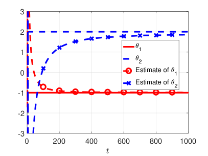
(a) Element-wise asymptotic convergence.

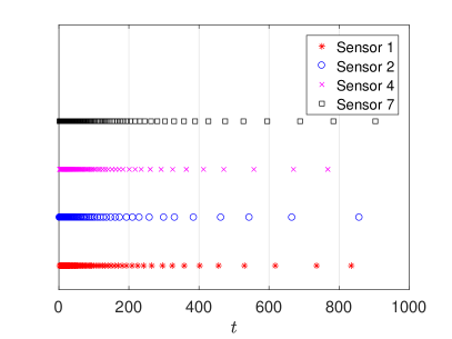
(b) Communication triggering instants of each sensor.

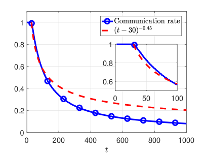
(c) Dynamics of communication rate $\lambda_{c}(t)$.

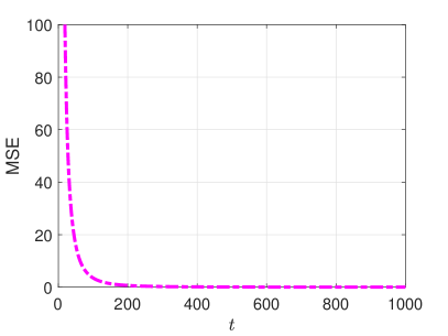
(d) Mean-square convergence.

Figure 2: Simulation results of Algorithm 1.

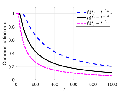
(a) Dynamics of communication rate $\lambda_{c}(t)$.

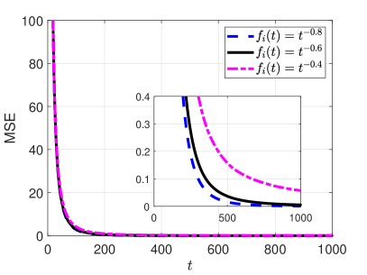
(b) Mean-square convergence.

Figure 3: Communication rate and MSE of Algorithm 1 under three triggering thresholds.

Under the above setting, we conduct a Monte Carlo experiment with $M_{0}=100$ runs for Algorithm 1 with $\alpha_{i}(t)=t^{-0.7}$, and $f_{i}(t)=t^{-0.5}$ for $i=1,2,\dots,7$. To evaluate the mean-square error, we define

$$\text{MSE}(t) =\frac{1}{NM_{0}}\sum_{j=1}^{M_{0}}\sum_{i=1}^{N}\left\lVert x_{i}^{j}(t)-\theta\right\rVert^{2},$$ (60)

where $x_{i}^{j}(t)$ is the estimate of $\theta$ by sensor $i$ at time $t$ in the $j$-th run. The simulation results are provided in FIG. 2. From FIG. 2(a), the average estimate of all sensors is asymptotically convergent to the true parameter vector. The event-triggered communication triggering instants of sensors 1, 2, 4, and 7 are provided in FIG. 2(b), where we can see less and less communications occur as time goes on. The communication rate is 0.08 in the interval $t=[0,1000]\cap\mathbb{N}$. The dynamics of the communication rate in the given interval is provided in FIG. 2(c), where the communication rate remains to be 1 from $t=1$ to $t=30$ meaning that sensors persistently communicate with each other. This is because at the initial time, much informative data can be used to update the sensor estimates. As time goes on, the communication rate is tending to zero, since sensors only transmits informative data which is becoming less. Moreover, in order to illustrate the convergence rate of the communication rate, we provide the dynamics of $(t-30)^{-0.45}$ for $t>30$. From FIG. 2(c), the communication rate asymptotically decays to zero faster than $(t-30)^{-0.45}$, corresponding to the results in Theorem 3.3. The mean-square convergence of the algorithm is illustrated in FIG. 2(d), corresponding to Theorem 3.1. Moreover, by choosing three triggering thresholds, i.e., $f_{i}(t)=t^{-0.8},t^{-0.6},t^{-0.4}$, we provide Fig. 3 for illustrating the influence of triggering threshold to communication rate and MSE. From this figure, for the threshold with a faster decreasing speed, the corresponding communication rate decays more slowly, while the MSE decays more quickly. This indicates that the threshold leads to a tradeoff between communication rate and MSE, corresponding to Remark 3.9.

5-B Example 2

In this example, we compare the proposed algorithm with three existing algorithms over a sensor network whose size is larger than that in example 1. Consider an undirected connected sensor network with 200 nodes for estimating a target position $\theta=[1,2,5]$. The sensor network topology is generated as a random geometric graph and provided in FIG. 4(a), where two types of sensors are deployed with the same number (i.e., 100) and denoted by black circle and red diamond. Assume for any $i=1,2,\dots,200$, the weight $a_{i,j}=1$, for $j\in\mathcal{N}_{i}$. The measurement matrices of black-circle and red-diamond sensors are assumed to be $H_{A}=[0,0,1]$ and $H_{B}=[1,0,0;0,1,0]$, respectively. Suppose the sensor noise follows a standard Gaussian process and is independent in both space and time.

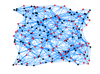
(a) Sensor network.

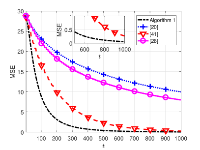
(b) MSE performance of four algorithms.

Figure 4: Comparison of four distributed algorithms over a sensor network with 200 nodes.

We compare Algorithm 1 with three typical distributed estimation algorithms in the literature, including the generalized linear unconstrained algorithm from [4], the diffusion least-mean squares algorithm from [38], and the distributed parameter algorithm from [7]. The parameters in our algorithm are $\alpha_{i}(t)=(t+100)^{-0.7}$, and $f_{i}(t)=t^{-0.5}$ for $i=1,2,\dots,200$. The parameters in the algorithm of [4] are $\alpha(t)=10/(t+1)^{0.7}$, $\beta(t)=0.1/(t+1)^{0.7}$, and $K=(\sum_{i=1}^{200}H_{i}^{T}H_{i})^{-1}$, where $H_{i}$ is the measurement matrix of sensor $i$. The parameters in the algorithm of [7] are $b(t)=(t+100)^{-0.7}$ and $a_{i,j}=1$, for $i,j=1,2,\dots,200$. The parameters in the algorithm of [38] are $\mu(t)=(t+100)^{-0.7}$ and $c_{i,j}=1/|\mathcal{N}_{i}+1|$ for $j\in\mathcal{N}_{i}\bigcup\{i\}$, $i=1,2,\dots,200$. The initial parameter estimate is zero for each algorithm. We compare our event-triggered algorithm with the above three time-triggered algorithms under the same communication rate $\lambda_{c}=0.09$. It means that for the three time-triggered algorithms, each sensor receives the messages from neighbors for every $11\approx 1/\lambda_{c}$ steps, before that they use the latest messages from neighbors to run the algorithms. Under this setting, we conduct a Monte Carlo experiment for running the four algorithms simultaneously with $100$ runs. With the MSE notation in (60), the performance of these algorithms are illustrated in FIG. 4(b). It shows that the outputs of all algorithms are convergent to the true parameter vector, and our event-triggered distributed algorithm outweighs other three algorithms in convergence speed under the same communication rate constraint.

6 Conclusion

In this paper, a distributed parameter estimation problem over a sensor network with event-triggered communications was studied. First, a fully distributed estimation algorithm was proposed based on an event-triggered communication scheme which determines when a sensor should share the parameter estimates with neighboring sensors. Then, under mild conditions, some main estimation properties of the algorithm including mean-square and almost-sure convergence were analyzed, respectively. The convergence rates were also estimated. Under some extra conditions, it was proved that the communication rate of the whole network using the proposed algorithm decays to zero almost surely as time goes to infinity, which indicates that a tremendous amount of redundant communications are avoided. It was also shown that adjusting the decay speed of the triggering threshold can lead to a tradeoff between the convergence rate of the estimation error and the decay speed of the communication rate. Future work can be done by considering more general models of systems and networks, such as nonlinear measurement models, time-varying, unbalanced, or stochastic graphs.

References

- [1] F. S. Cattivelli, C. G. Lopes, and A. H. Sayed, “Diffusion recursive least-squares for distributed estimation over adaptive networks,” IEEE Trans. Signal Process., vol. 56, no. 5, pp. 1865–1877, 2008.
- [2] F. S. Cattivelli and A. H. Sayed, “Diffusion LMS strategies for distributed estimation,” IEEE Trans. Signal Process., vol. 58, no. 3, pp. 1035–1048, 2010.
- [3] K. R. Rad and A. Tahbaz-Salehi, “Distributed parameter estimation in networks,” in IEEE Conference on Decision and Control, pp. 5050–5055, 2010.
- [4] S. Kar and J. M. Moura, “Convergence rate analysis of distributed gossip (linear parameter) estimation: Fundamental limits and tradeoffs,” IEEE J. Sel. Top. in Signal Process., vol. 5, no. 4, pp. 674–690, 2011.
- [5] S. Kar, J. M. Moura, and K. Ramanan, “Distributed parameter estimation in sensor networks: Nonlinear observation models and imperfect communication,” IEEE Trans. Inform. Theory, vol. 58, no. 6, pp. 3575–3605, 2012.
- [6] S. Kar, J. M. Moura, and H. V. Poor, “Distributed linear parameter estimation: Asymptotically efficient adaptive strategies,” SIAM J. Control Optim., vol. 51, no. 3, pp. 2200–2229, 2013.
- [7] Q. Zhang and J.-F. Zhang, “Distributed parameter estimation over unreliable networks with Markovian switching topologies,” IEEE Trans. Automat. Control, vol. 57, no. 10, pp. 2545–2560, 2012.
- [8] J. Haupt, R. M. Castro, and R. Nowak, “Distilled sensing: Adaptive sampling for sparse detection and estimation,” IEEE Trans. Inform. Theory, vol. 57, no. 9, pp. 6222–6235, 2011.
- [9] R. M. Castro and E. Tánczos, “Adaptive sensing for estimation of structured sparse signals,” IEEE Trans. Inform. Theory, vol. 61, no. 4, pp. 2060–2080, 2015.
- [10] M. A. Davenport, A. K. Massimino, D. Needell, and T. Woolf, “Constrained adaptive sensing,” IEEE Trans. Signal Process., vol. 64, no. 20, pp. 5437–5449, 2016.
- [11] M. Rabi, G. V. Moustakides, and J. S. Baras, “Adaptive sampling for linear state estimation,” SIAM Journal on Control and Optimization, vol. 50, no. 2, pp. 672–702, 2012.
- [12] B. Sinopoli, L. Schenato, M. Franceschetti, K. Poolla, M. I. Jordan, and S. S. Sastry, “Kalman filtering with intermittent observations,” IEEE Trans. Automat. Control, vol. 49, no. 9, pp. 1453–1464, 2004.
- [13] J. Wu, Q.-S. Jia, K. H. Johansson, and L. Shi, “Event-based sensor data scheduling: Trade-off between communication rate and estimation quality,” IEEE Trans. Automat. Control, vol. 58, no. 4, pp. 1041–1046, 2012.
- [14] K. You, L. Xie, and S. Song, “Asymptotically optimal parameter estimation with scheduled measurements,” IEEE Trans. Signal Process., vol. 61, no. 14, pp. 3521–3531, 2013.
- [15] D. Han, K. You, L. Xie, J. Wu, and L. Shi, “Optimal parameter estimation under controlled communication over sensor networks.,” IEEE Trans. Signal Process., vol. 63, no. 24, pp. 6473–6485, 2015.
- [16] J.-D. Diao, J. Guo, and C.-Y. Sun, “Event-triggered identification of FIR systems with binary-valued output observations,” Automatica J. IFAC, vol. 98, pp. 95–102, 2018.
- [17] M. Muehlebach and S. Trimpe, “Distributed event-based state estimation for networked systems: An lmi approach,” IEEE Trans. Automat. Control, vol. 63, no. 1, pp. 269–276, 2017.
- [18] G. Battistelli, L. Chisci, and D. Selvi, “A distributed Kalman filter with event-triggered communication and guaranteed stability,” Automatica J. IFAC, vol. 93, pp. 75–82, 2018.
- [19] X. He, C. Hu, Y. Hong, L. Shi, and H.-T. Fang, “Distributed Kalman filters with state equality constraints: Time-based and event-triggered communications,” IEEE Trans. Automat. Control, vol. 65, no. 1, pp. 28–43, 2020.
- [20] X. Ge, Q.-L. Han, X.-M. Zhang, L. Ding, and F. Yang, “Distributed event-triggered estimation over sensor networks: A survey,” IEEE Trans. on Cybernet, vol. 50, no. 3, pp. 1306–1320, 2019.
- [21] X. Cao and T. Basar, “Decentralized online convex optimization with event-triggered communications,” IEEE Trans. Signal Process., vol. 69, pp. 284–299, 2021.
- [22] H. Li, S. Liu, Y. C. Soh, and L. Xie, “Event-triggered communication and data rate constraint for distributed optimization of multiagent systems,” IEEE Trans. on Syst., Man, and Cybernet.: Systems, vol. 48, no. 11, pp. 1908–1919, 2017.
- [23] W. Chen and W. Ren, “Event-triggered zero-gradient-sum distributed consensus optimization over directed networks,” Automatica J. IFAC, vol. 65, pp. 90–97, 2016.
- [24] J. Wang, T. Li, and X. Zhang, “Decentralized cooperative online estimation with random observation matrices, communication graphs and time delays,” IEEE Trans. Inform. Theory, vol. 67, no. 6, pp. 4035–4059, 2021.
- [25] J. Lei and H.-F. Chen, “Distributed estimation for parameter in heterogeneous linear time-varying models with observations at network sensors,” Commun. Inf. Syst., vol. 15, no. 4, pp. 423–451, 2015.
- [26] Y. Chen, S. Kar, and J. M. Moura, “Resilient distributed field estimation,” SIAM J. Control Optim., vol. 58, no. 3, pp. 1429–1456, 2020.
- [27] X. He, Q. Liu, J. Wu, and K. H. Johansson, “Distributed parameter estimation under event-triggered communications,” in Chinese Control Conference, pp. 5888–5893, IEEE, 2019.
- [28] F. S. Cattivelli and A. H. Sayed, “Distributed nonlinear Kalman filtering with applications to wireless localization,” in IEEE International Conference on Acoustics Speech and Signal Processing, pp. 3522–3525, 2010.
- [29] R. Olfati-Saber and R. M. Murray, “Consensus problems in networks of agents with switching topology and time-delays,” IEEE Trans. Automat. Control, vol. 49, no. 9, pp. 1520–1533, 2004.
- [30] S. Kar and J. M. Moura, “Gossip and distributed Kalman filtering: Weak consensus under weak detectability,” IEEE Trans. Signal Process., vol. 59, no. 4, pp. 1766–1784, 2011.
- [31] M. Mehran and E. Magnus, Graph theoretic methods in multiagent networks. Princeton University Press, 2010.
- [32] L. Guo, “Stability of recursive stochastic tracking algorithms,” SIAM Journal on Control and Optimization, vol. 32, no. 5, pp. 1195–1225, 1994.
- [33] A. S. Poznyak, Advanced Mathematical Tools for Automatic Control Engineers: Stochastic Techniques. Elsevier, 2009.
- [34] H.-F. Chen, Stochastic Approximation and Its Applications. Kluwer, Boston, MA, 2002.
- [35] L. Guo, “Estimating time-varying parameters by the Kalman filter based algorithm: Stability and convergence,” IEEE Trans. Automat. Control, vol. 35, no. 2, pp. 141–147, 1990.
- [36] T. Li and J. Wang, “Distributed averaging with random network graphs and noises,” IEEE Trans. Inform. Theory, vol. 64, no. 11, pp. 7063–7080, 2018.
- [37] I. S. Gradshteyn and I. M. Ryzhik, Table of integrals, series, and products. Academic press, 2014.
- [38] C. G. Lopes and A. H. Sayed, “Diffusion least-mean squares over adaptive networks: Formulation and performance analysis,” IEEE Trans. Signal Process., vol. 56, no. 7, pp. 3122–3136, 2008.