Magnetic phases for two $t_{2g}$ holes with spin-orbit coupling and crystal field

Abstract

We investigate two holes in the the $t_{2g}$ levels of a square-lattice Mott insulator with strong spin-orbit coupling. Exact diagonalization of a spin-orbital model valid at strong onsite interactions, but arbitrary spin-orbit coupling and crystal field is complemented by an effective triplon model (valid for strong spin-orbit coupling) and by a semiclassical variant of the model. We provide the magnetic phase diagram depending on crystal field and spin-orbit coupling, which largely agrees for the semiclassical and quantum models, as well as excitation spectra characterizing the various phases.

I Introduction

The interplay between spin-orbit coupling (SOC) and correlated electrons as a driving force of physical properties in transition metal compounds has gathered significant interest in the last decade [1, 2]. The manifold of competing interactions in these materials has led to a plethora of interesting properties like topological Mott insulators, superconductivity and spin liquids [3].

Focus was first on materials with one hole in the $t_{2g}$ manifold and strong SOC in addition to sizable correlations, as realized in $4d$ and $5d$ states. SOC couples spin $\textbf{S}=1/2$ and orbital $\textbf{L}=1$ degrees of freedom to a total angular moment $\textbf{J}=1/2$, so that the model in the end can be described by an effective half-filled model. In addition to similarities to high-$T_{C}$ cuprates and the potential realization [4] of the exactly solvable Kitaev model [5] in a honeycomb lattice, which have stimulated extensive research on these compounds [6, 7], potential applications in spintronics have been proposed more recently [8].

Interest was then extended to other fillings [9, 10], and we will here focus on the Mott-insulating state for two holes. For dominant SOC (as possibly in Ir), the system is in the $j$-$j$ limit and the groundstate is thus likely a nonmagnetic ground state [11, 12] given by two holes filling the $j=1/2$ states. For weaker SOC, e.g. in ruthenates, L-S coupling is more appropriate, where SOC couples $\textbf{L}=1$ and $\textbf{S}=1$ to $\textbf{J}=0$, again leading to a nonmagnetic ground state for a single ion [13]. However, energy scales are here rather different with a much smaller splitting between the singlet and triplet states. When going from an isolated ion to a compound with a lattice, competing processes can overcome the splitting. Superexchange mixes in states from the $\textbf{J}=1$ level, which can lead to a magnetic ground state.

This phenomenon is also known as excitonic or Van-Vleck magnetism [14], and has for instance been proposed to provide a route to a bosonic Kitaev-Heisenberg model [15, 16] and to explain magnetic excitations of $\text{Ca}_{2}\text{RuO}_{4}$ [17]. In one dimension, density-matrix renormalization group has been applied to a spin-orbit coupled and correlated $t_{2g}$ model with two holes, and antiferromagnetic (AFM) order has been found [18, 19] both for intermediate correlations (of a more ’standard’ excitonic type with intersite pairs) and for strong correlations (of the ’onsite’ type discussed in Ref. [14]). Similarly, dynamical mean-field theory has yielded excitonic antiferromagnetism in a two-dimensional model [20].

A material which has been a focal point of discussions in this context is $\text{Ca}_{2}\text{RuO}_{4}$. In neutron scattering experiments an in-plane AFM ordering has been measured below the Néel temperature $T_{N}\approx 110\,K$ and neutron-scattering spectra can only be explained by taking into account substantial SOC [21, 22, 23, 24]. Accordingly, excitonic magnetism, where the magnetic moment arises from admixture of $\textbf{J}=1$ component into the ionic $\textbf{J}=0$ state, has been argued to describe this compound [21, 17]. However, a strong crystal field (CF), favoring doubly occupied $xy$ orbitals, is also clearly present in Ca₂RuO₄ and complicates the analysis, because it would favor a description in terms of a spin-one system. This is backed by a structural phase transition accompanying the metal-insulator transition. SOC would in this picture be only a correction affecting excitations [24, 25].

In a previous publication, some of us have used the variational cluster approach (VCA) based on ab initio parameters to show that excitonic antiferromagnetism can coexist with substantial CF’s and that Ca₂RuO₄ falls into this regime [26, 27] of orbitally polarized excitonic antiferromagnetism. In the present paper, we study the competition of CF $\Delta$ and SOC $\lambda$ in $t_{2g}^{4}$ systems in more depth and for a wider parameter space. We investigate an effective spin-orbit model obtained in second-order perturbation theory, as also used for $\text{Ca}_{2}\text{RuO}_{4}$ [26]. This extends the comparison of CF and SOC acting on the itinerant regime (without magnetic ordering) [10] to magnetic Mott insulators. Our work is also complementary to a very recent study using the Hartree-Fock approach to investigate the dependence of magnetic ordering on SOC, CF, and tilting of octahedra, which focused on patterns with smaller unit cells of one or two Ca ions [28]. We obtain $\Delta$-$\lambda$ phase diagrams using both Monte-Carlo (MC) simulations for the semiclassical limit of the model and exact diagonalization (ED) for the quantum system and provide excitation spectra for the various magnetic phases.

As expected [26], stripy magnetism is found when both SOC and CF are weak, and checkerboard order (as seen in Ca₂RuO₄) takes over when either becomes strong enough to sufficiently lift orbital degeneracy. For negative CF, i.e., disfavoring doubly occupied $xy$ orbitals, we find an additional intermediate phase with rather complex magnetic order. Overall, we find the agreement between the semiclassical and quantum models to be quite good, with phase boundaries between the magnetic phases only moderately different. Similarly, the transition to a paramagnetic (PM) state at strong SOC in the full quantum-mechanical model is compared to an effective triplon model [14], valid at strong SOC, and found to agree. Finally, we present the dynamic spin structure factor of the spin-orbital model to discuss signatures of the various magnetic phases accessible to neutron scattering experiments.

In Sec. II, we introduce models, i.e., the full spin-orbital superexchange model as well as the triplon model valid for strong SOC, and methods. In Sec. III.1, we first go over the limiting cases of the spin-orbital system at dominant CF, the triplon scenario, discuss the intricate interplay of spin and orbital order for small CF and SOC, and finally give the phase diagram for intermediate values in Sec. III.2. The phase diagram is compared to results of semiclassical MC calculations for the same model in Sec. III.3. Section III.4 presents the dynamic-spin-structure-factor data corresponding to neutron scattering experiments for the various phases. Finally Sec. IV gives a summary of the results found in this paper.

II Model and Methods

II.1 Spin-orbit model

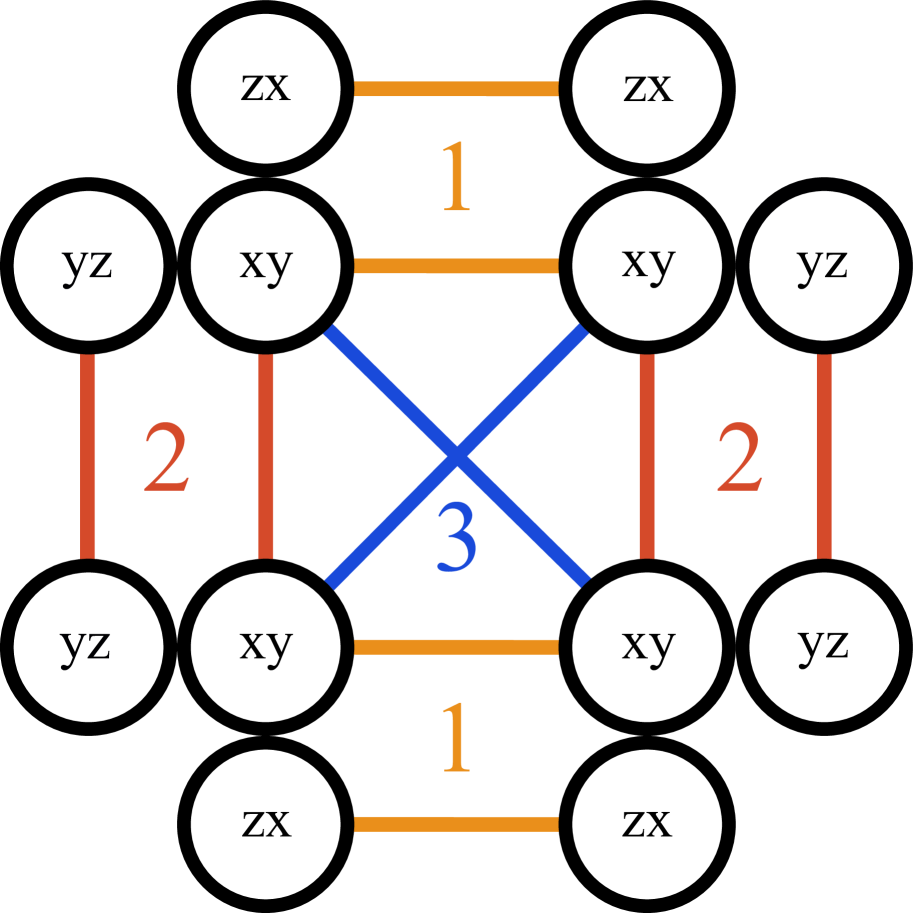
[0.5] [0.43] $t_{\alpha,m}$ Amplitude $t_{xy,1}$ $t_{xy}$ $t_{xy,2}$ $t_{xy}$ $t_{xy,3}$ $t_{\text{NNN}}$ $t_{zx,1}$ $t_{zx}$ $t_{zx,2}$ $0$ $t_{zx,3}$ $0$ $t_{yz,1}$ $0$ $t_{yz,2}$ $t_{yz}$ $t_{yz,3}$ $0$

Figure 1: Possible hopping processes in $\text{Ca}_{2}\text{RuO}_{4}$ (based on [26]). The $xy$ orbital can hop in $x$- (bond 1) and $y$-direction (bond 2) and has a nonzero hopping amplitude for next-nearest neighbors (bond 3). The $zx$ and $yz$ orbital can hop only on bond 1 and 2 respectively.

Figure 2: Possible hopping parameters $t_{\alpha,m}$ from equations (1) and (II.1)-(II.1) as well as their amplitudes for a square lattice geometry. The parameter $m$ here indicates the bond type introduced in Fig.2 while $\alpha$ are the $t_{2g}$ orbitals.

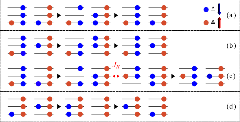
Figure 3: Displayed are the different possible hopping processes from (II.1) and (II.1). In (a) and (b) virtual hoppings where the orbital configuration is preserved are shown. In (a) the double occupancy is at the same orbital, while in (b) the double occupancy resides at different orbitals. (c) and (d) display second order hoppings where the orbital configurations change. In the “pair-flip” process (c) the change arises due to the last term in (II.1), while the “swap” process (d) arises due to a different orbital hopping back then forth.

$\text{Ca}_{2}\text{RuO}_{4}$ has a $d^{4}$ configuration, meaning that four electrons reside in three $t_{2g}$ orbitals, from now on referred to as $xy$-, $zx$-, and $yz$-orbital. The kinetic part of this Hamiltonian can be written as

$$H_{\text{kin}} =\sum_{m=1}^{3}\sum_{\braket{i,j}_{m}}\sum_{\alpha,\sigma}(t_{\alpha,m}c_{i,\alpha,\sigma}^{\dagger}c_{j,\alpha,\sigma}+h.c.),$$ (1)

where $m$ are the three different bond types introduced in Fig. 2 and $t_{\alpha,m}$ is the hopping amplitude depending on the orbital flavor $\alpha$ and the bond type $m$. Tab. 2 gives the amplitudes for all possible $t_{\alpha,m}$ for a square lattice geometry. $c_{i,\alpha,\sigma}^{\dagger}$ ($c_{i,\alpha,\sigma}$) is creating (annihilating) an electron in orbital $\alpha$ at site $i$ with spin $\sigma$. The possible hopping paths for $\text{Ca}_{2}\text{RuO}_{4}$ [26, 29] are shown in Fig. 2. On nearest neighbor bonds (NN) only two orbitals are active (e.g. $xy$ and $zx$ for $x$-bonds), while for next-nearest neighbor bonds (NNN) only the $xy$ orbital has a nonzero hopping amplitude (see Tab. 2).

The onsite interaction has the form of a Kanamori-Hamiltonian [30]

$$H_{\text{int}}= U\sum_{i,\alpha}n_{i\alpha\uparrow}n_{i\alpha\downarrow}+U^{\prime}\sum_{i,\sigma}\sum_{\alpha<\beta}n_{i\alpha\sigma}n_{i\beta\,-\sigma}$$

$$+(U^{\prime}-J_{H})\sum_{i,\sigma}\sum_{\alpha<\beta}n_{i\alpha\sigma}n_{i\beta\sigma}$$

$$-J_{H}\sum_{i,\alpha\neq\beta}(c_{i\alpha\uparrow}^{\dagger}c_{i\alpha\downarrow}c_{i\beta\downarrow}^{\dagger}c_{i\beta\uparrow}-c_{i\alpha\uparrow}^{\dagger}c_{i\alpha\downarrow}^{\dagger}c_{i\beta\downarrow}c_{i\beta\uparrow}),$$ (2)

with intraorbital Hubbard interaction $U$, interorbital $U^{\prime}=U-2J_{H}$ and Hund’s coupling $J_{H}$.

Since the computational cost to calculate this Hamiltonian via ED is very high we only consider a low energy sector of our Hilbert space. We focus here on the Mott-insulating regime with large $U$ and $J_{H}$. The low-energy sector is then given by states where each site contains exactly four electrons (two holes), as $U$ suppresses charge fluctuations. Hund’s-rule coupling $J_{H}$ moreover ensures that exactly one orbital per site is doubly occupied and that the electrons in the remaining two half-filled orbitals form a total spin $\mathbf{S}=1$. This means we have three different orbital configurations and a $\mathbf{S}=1$ spin state, leading to a subspace of nine states. The orbital configurations are labeled with the orbital which is doubly occupied from here on. It turns out (see [31]) that this orbital degree of freedom can be mapped to an effective angular momentum with

$$L^{x}=\mathcal{L}_{yz}=-\text{i}(\ket{xy}\bra{zx}-\ket{zx}\bra{xy})$$

$$L^{y}=\mathcal{L}_{xz}=-\text{i}(\ket{yz}\bra{xy}-\ket{xy}\bra{yz})$$

$$L^{z}=\mathcal{L}_{xy}=-\text{i}(\ket{zx}\bra{yz}-\ket{yz}\bra{zx}),$$ (3)

where the notation $\mathcal{L}_{\alpha}$ with an orbital index $\alpha$ is introduced to make the expression of equations (II.1)-(II.1) more straightforward and can be easily translated into the $x$-, $y$- and $z$-component of the angular momentum $\mathbf{L}$.

The effective spin-orbital Hamiltonian is then obtained by treating the hopping term in second order perturbation theory. This gives a Kugel-Khomskii type Hamiltonian [32, 33], where only virtual hopping processes of the form $d^{4}d^{4}\rightarrow d^{5}d^{3}\rightarrow d^{4}d^{4}$ take place. The effective spin-orbital superexchange Hamiltonian includes both orbital as well as spin-orbital interactions. Spin-orbital superexchange terms that preserve orbital occupations of the two sites are

$$H_{\text{OP}}= \sum_{m=1}^{3}\sum_{\braket{i,j}_{m}}\sum_{\alpha\neq\beta}\bigg{[}t_{\beta,m}^{2}\frac{U+J_{H}}{U(U+2J_{H})}$$

$$\times(\mathbf{S}_{i}\mathbf{S}_{j}-1)(1-\mathcal{L}_{\alpha}^{2})_{i}(1-\mathcal{L}_{\alpha}^{2})_{j}$$

$$+\bigg{(}t_{\gamma\neq(\alpha,\beta),m}^{2}\frac{(U+J_{H})}{U(U+2J_{H})}-\frac{(t_{\alpha,m}^{2}+t_{\beta,m}^{2})J_{H}}{U(U-3J_{H})}\bigg{)}$$

$$\times(\mathbf{S}_{i}\mathbf{S}_{j}-1)(1-\mathcal{L}_{\alpha}^{2})_{i}(1-\mathcal{L}_{\beta}^{2})_{j}\bigg{]}.$$ (4)

Here we used the aforementioned mapping from orbitals to effective angular momentum $\mathbf{L}$. Having two orbitals of the same flavor means only the electrons in the other two orbitals are allowed to perform a virtual hopping (Fig.3 (a)), while for different flavors each orbital can be involved in such a hopping process (Fig.3 (b)).

Furthermore, there are spin-orbital couplings that change orbital configurations. These can be separated in so called “pair-flip” (Fig.3 (c)) processes where two orbitals of the same flavor flip their flavor to another one and “swap” processes (Fig.3 (d)) where two orbitals of different flavor exchange their flavor

$$H_{\text{OF}}= \sum_{m=1}^{3}\sum_{\braket{i,j}_{m}}\sum_{\alpha\neq\beta}\bigg{[}-t_{\alpha,m}t_{\beta,m}\frac{J_{H}}{U(U+2J_{H})}$$

$$\times(\mathbf{S}_{i}\mathbf{S}_{j}-1)(\mathcal{L}_{\beta}\mathcal{L}_{\alpha})_{i}(\mathcal{L}_{\beta}\mathcal{L}_{\alpha})_{j}$$

$$+\bigg{(}t_{\alpha,m}t_{\beta,m}\frac{(U-J_{H})}{U(U-3J_{H})}\bigg{)}$$

$$\times(\mathbf{S}_{i}\mathbf{S}_{j}+1)(\mathcal{L}_{\beta}\mathcal{L}_{\alpha})_{i}(\mathcal{L}_{\alpha}\mathcal{L}_{\beta})_{j}\bigg{]}.$$ (5)

Finally, additional orbital terms affect sites $i$ and $j$ with different orbital occupation:

$$H_{\mathbf{L}\cdot\mathbf{L}}= \sum_{m=1}^{3}\sum_{\braket{i,j}_{m}}\sum_{\alpha\neq\beta}\bigg{[}t_{\alpha,m}t_{\beta,m}\frac{2J_{H}}{U(U-3J_{H})}$$

$$\times(\mathcal{L}_{\beta}\mathcal{L}_{\alpha})_{i}(\mathcal{L}_{\alpha}\mathcal{L}_{\beta})_{j}$$

$$-(t_{\alpha,m}^{2}+t_{\beta,m}^{2})\frac{1}{(U-3J_{H})}$$

$$\times(1-\mathcal{L}_{\alpha}^{2})_{i}(1-\mathcal{L}_{\beta}^{2})_{j}\bigg{]}.$$ (6)

The full superexchange interaction of two sites can be summarized as

$$H=H_{\text{OF}}+H_{\text{OP}}+H_{\mathbf{L}\cdot\mathbf{L}}$$ (7)

Using the hoppings symmetry allowed on a square lattice up to second neighbors (see Fig. 2 and Tab. 2), one obtains the effective spin-orbital model that can, e.g., be applied to $\text{Ca}_{2}\text{RuO}_{4}$ [26].

In addition to these intersite interactions we also include SOC $\lambda$ and the CF splitting $\Delta$. The SOC terms can be written in the form

$$H_{\text{SOC}}=\lambda\sum_{i}\mathbf{S}_{i}\cdot\mathbf{L}_{i}=\text{i}\lambda\sum_{i}\sum_{\begin{subarray}{c}\alpha,\beta,\gamma\\ \sigma,\sigma^{\prime}\end{subarray}}\epsilon_{\alpha\beta\gamma}\tau^{\alpha}_{\sigma\sigma^{\prime}}c^{\dagger}_{i,\beta,\sigma}c_{i,\gamma,\sigma^{\prime}},$$ (8)

where $\epsilon_{\alpha\beta\gamma}$ denotes the Levi-Civita symbol and $\tau^{\alpha}$ are Pauli matrices [10, 34]. SOC favors the total angular momentum to be $J=0$, while the CF favors a double occupancy of the $xy$ orbital. Projected onto the low-energy Hilbert space spanned by $\mathbf{S}=1$ and $\mathbf{L}=1$, they can be written as

$$H_{\text{Ion}}=H_{\text{SOC}}+H_{\text{CF}}=\lambda\sum_{i}\mathbf{S}_{i}\mathbf{L}_{i}+\Delta\sum_{i}(L^{z}_{i})^{2}.$$ (9)

Going beyond previous effective models [14, 35, 36], our model thus fully captures the influence of the Hund’s coupling $J_{H}$ and gives the possibility to investigate anisotropic hoppings as well as the $\lambda,\Delta\rightarrow 0$ limits.

The competition between the last two terms, CF $\Delta$ and SOC $\lambda$, is one of the main topics of this paper. We thus fix the remaining parameters to values appropriate for Ca₂RuO₄ [37]. Hopping processes between NN sites and NNN sites were included with hopping parameters set to $t_{xy}=0.2\,\text{eV}$, $t_{yz}=t_{zx}=0.137\,\text{eV}$, $t_{\text{NNN}}=0.1\,\text{eV}$, and $\Delta=0.25\,\text{eV}$ via density-functional theory [37]. However, we found that results only differ in details when more symmetric NN hoppings $t_{xy}=t_{yz}=t_{zx}$ are used or when NNN hopping is left off. Substantial onsite Coulomb repulsion and Hund’s-rule coupling $U=2\,\text{eV}$ and $J_{H}=0.34\,\text{eV}$, as can be inferred from x-ray studies [38], stabilize a Mott insulator with robust onsite spin $\mathbf{S}=1$. Previous calculations using the VCA have shown [26] that most of the weight of the ground state is indeed captured by states that minimize Coulomb interactions (II.1), so that a super-exchange treatment and the resulting spin-orbital model can be justified.

II.2 PM phase and triplon model

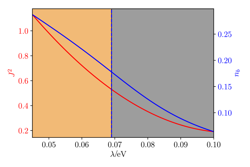
Figure 4: $\braket{J^{2}}$ of the spin-orbit model (red) and triplon number $n_{b}$ of the triplon model (blue) are plotted in dependency of SOC $\lambda$. The dashed blue line denotes the phase transition to the PM phase in the triplon model, which is determined via $\frac{d^{2}n_{b}}{d\lambda^{2}}=0$. The parameters are chosen to be $t_{xy}=0.2\,\text{eV},\,t_{yz}=t_{zx}=0.137\,\text{eV},\,t_{\text{NNN}}=0.1\,\text{eV}$, $U=2\,\text{eV}$, $J_{H}=0.34\,\text{eV}$, and $\Delta=0.1\,\text{eV}$.

For strong SOC, we expect our system to be in a PM phase where each ion is in the $J=0$ state [14, 26]. Transition into magnetically ordered states occurs then via condensation of triplons. We are going to compare the large-SOC limit of the full spin-orbit superexchange model to a triplon model appropriate for significant SOC. We take an approach like in Ref. [36] and project (II.1)-(II.1) onto the low energy subspace of the SOC Hamiltonian, i.e., onto the $J=0$ and $J=1$ states

$$\ket{J=0,M_{J}=0}=\frac{1}{\sqrt{3}}(\ket{M_{S}=1,M_{L}=-1}+\ket{-1,1}-\ket{0,0})$$

$$\ket{J=1,M_{J}=1}=\frac{1}{\sqrt{2}}(\ket{1,0}-\ket{0,1})$$

$$\ket{J=1,M_{J}=0}=\frac{1}{\sqrt{2}}(\ket{1,-1}-\ket{-1,1})$$

$$\ket{J=1,M_{J}=-1}=\frac{1}{\sqrt{2}}(\ket{-1,0}-\ket{0,-1})$$ (10)

and projecting out the $J=2$ levels.

We then can define triplon operators $T_{1/0/-1}^{\dagger}$ ($T_{1/0/-1}$) which create (annihilate) the respective $J=1$ triplet state and annihilate (create) the $J=0$ singlet. These operators can then be rewritten to $T_{x/y/z}$ (for further details see [14]).

II.3 Methods

To investigate these models we use ED on an eight site cluster with $\sqrt{8}\times\sqrt{8}$ geometry to determine a $\Delta-\lambda$ phase diagram as well as the dynamical spin structure factor (DSSF) for specific $\Delta$ and $\lambda$.

This is done for both the full spin-orbital model (Sec. II.1) as well as the triplon model introduced in Sec. II.2. While the spin-orbital model is capable of capturing the physics at weak SOC, for strong SOC the triplon model is numerically more accessible due to the reduction of the Hilbert space.

To confirm the results of ED and get a better understanding of the phases identified, we additionally performed semiclassical parallel tempering MC calculations with the full spin-orbital model for a $4\times 4$ cluster. The easier approach of a fully classical treatment, meaning a parametrization of $\textbf{S}_{i}$ and $\textbf{L}_{i}$ as three dimensional real vectors, is not sufficient here. A simple example can be found in the $(\mathcal{L}_{\beta}\mathcal{L}_{\alpha})_{i}$ terms in the Hamiltonian. There is a clear difference between calculating this expression with scalar components of a three dimensional vector and representing the angular momenta as non-commutative matrices. We accomplish the latter by instead considering trial wave functions of direct-product form

$$\ket{\Psi}=\operatorname*{\text{\raisebox{1.07639pt}{\scalebox{0.8}{$\bigotimes$}}}}_{i}\left(\ket{S_{i}}\otimes\ket{L_{i}}\right)\;,$$ (11)

where the first product runs over all sites $i$. We allow all complex linear combinations of the $L^{z}$ eigenvalues $\ket{L_{i}}=\mu_{1,i}\ket{M_{L}=-1}+\mu_{2,i}\ket{M_{L}=0}+\mu_{3,i}\ket{M_{L}=+1}$ with $\boldsymbol{\mu}_{i}^{T}\boldsymbol{\mu}_{i}^{*}=1$, and analogously for the spin $\ket{S_{i}}$. These trial wave functions are used to calculate the energy, i.e., the energy becomes a (real-valued) function of classical complex vectors $\boldsymbol{\mu}_{i}$. Classical Markov-chain Monte Carlo is then based on this energy function.

A similar approach has been used for quadrupole correlations in a spin-1 model with biquadratic interaction  [39]. In this context one might refer to our method as a $SU(3)\otimes SU(3)$ semiclassical Monte-Carlo simulation. Compared to ED the numerical expenses of this method are minute. A big drawback of the product state nature of the basis is its inability to accurately represent the singlet and hence find the paramagnetic phase. However, we have the triplon model to confirm ED data in this parameter range. The Monte Carlo code is used as a counterpart of the triplon model for low spin-orbit coupling.

Finally we point out that all terms in the Hamiltonian are represented as matrices in the chosen basis and the scalar definitions of spin components or other observables are recovered by simply constructing the expectation values regarding $\ket{\Psi}$.

III Results

III.1 Limiting regimes

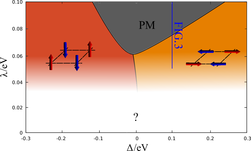
Figure 5: Phase diagram for large SOC in the triplon model introduced in Sec. II.2. The parameters are chosen to be $t_{xy}=0.2\,\text{eV},\,t_{yz}=t_{zx}=0.137\,\text{eV},\,t_{\text{NNN}}=0.1\,\text{eV}$, $U=2\,\text{eV}$, and $J_{H}=0.34\,\text{eV}$. For large SOC, the $J=0$ phases arises where no triplons are prevalent, while for $\Delta<0$ the z-AFM and for $\Delta>0$ the $xy$-AFM phase is favored.

III.1.1 $\Delta\gg\lambda$ Limit

Presumably the most straightforward limit of the $t_{2g}^{4}$ model is the case of dominant CF $\Delta\gg\lambda$ favoring the $xy$ orbital to be fully occupied. The two remaining orbitals $zx$ and $yz$ are then half filled and form a spin one. Magnetic ordering within the plane is then determined by the ratio of NNN and NN superexchange, with the latter usually dominating and favoring a checkerboard pattern.

III.1.2 $\lambda\gg\Delta$ Limit

For dominant SOC $\lambda\gg\Delta$, the ground state becomes the $J=0$ state without magnetic moment and therefore leads to a PM phase. Decreasing SOC leads to the possibility of an admixture of the $J=1$ states to the ground state, since the energy gap between the $J$ states is decreasing and superexchange is driving the transition between the $J=0$ and the $J=1$ states [14, 15, 14]. This triplon-condensation transition leads to a finite magnetization and magnetic ordering can be described with the triplon model introduced in Sec. II.2.

The transition from a magnetically ordered state to the PM state is seen in Fig. 4, which shows the triplon number obtained using ED for the triplon model on a $\sqrt{8}\times\sqrt{8}$ cluster. CF is here set to $\Delta=0.1\;\textrm{eV}$, where the magnetic order has a checkerboard pattern. The inflection point of the triplon number vs. SOC $\lambda$ (at $\lambda\approx 0.07\,$eV) was taken as the phase boundary to the PM phase. Figure 4 also shows the expectation value $\braket{J^{2}}$ obtained for the full spin-orbital superexchange model. While there is no obvious signal, like, e.g., an inflection point, for the phase boundary, increasing $\lambda$ leads to a decrease of $\braket{J^{2}}$, in agreement with the triplon number. Figure 5 gives the $\Delta$-$\lambda$ phase diagram for the triplon model at intermediate to large $\lambda$, where it can be assumed to be valid. Magnetic order switches from in-plane to out-of-plane at $\Delta\approx 0$, and the phase diagram is in qualitative agreement with [35] for $\Delta\geq 0$, where $J_{H}=0$ and isotropic hopping were used. The triplon model is naturally not able to capture the physical behavior for small SOC. From here on we will therefore focus on performing our calculations with the full spin-orbital model.

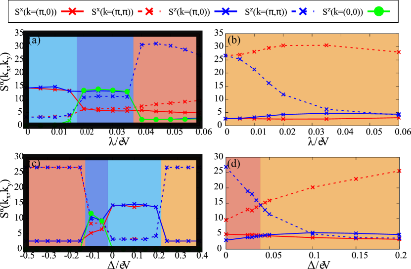
Figure 6: In-plane- ($x$-$y$) and out-of-plane ($z$) SSF $\text{S}^{\alpha}(k,\lambda,\Delta)$. $\lambda$ is varied in (a) with $\Delta=0\,\text{eV}$ and (b) with $\Delta=0.25\,\text{eV}$. $\Delta$ is varied in (c) with $\lambda=0$ and (d) with $\lambda=0.06\,\text{eV}$. The momenta $\mathbf{k}$ accessible on an $\sqrt{8}\times\sqrt{8}$ cluster are $\mathbf{k}=(0,0)$, $(\pi,0)$, $(0,\pi)$, $(\pm\tfrac{\pi}{2},\pm\tfrac{\pi}{2})$ and $(\pi,\pi)$. Remaining parameters are given in Sec. II.1.

III.1.3 $\lambda=0$ Limit

The opposite limit of $\lambda=0$ has been investigated for varied Coulomb repulsion $U$ and Hund’s coupling $J_{H}$ [40]. The calculations in [40] were done with a full nonperturbative treatment of the Hubbard-like Hamiltonian, which limited the cluster size to $2\times 2$. In agreement with our results, obtained with the full spin-orbital model, large orbital degeneracy at small CF $0\lesssim\Delta\lesssim 0.24\;\textrm{eV}$ leads to a complex stripy spin-orbital pattern [40, 26]. For larger positive $\Delta\gtrsim 0.24\;\textrm{eV}$, CF dominates and double occupancy is uniformly in the $xy$ orbital. Therefore the Hamiltonian reduces to orbital-preserving terms which yield a simple Heisenberg spin Hamiltonian, while NNN interactions are frustrated. These effects cause a phase transition from the stripy phase to a checkerboard pattern.

The magnetic ordering can be inferred from the spin structure factors (SSF) for $\lambda=0$ and variable CF that are summarized in Fig. 6 (c). In addition to the stripy and $xy$-polarized checkerboard patterns seen for $\Delta\gtrsim 0$, we find checkerboard order again for $\Delta\ll 0$. In this negative-$\Delta$ regime, the $xy$ orbital is half filled to gain in-plane kinetic (resp. superexchange) energy, while double occupation of $xz$ and $yz$ orbitals alternate in a checkerboard pattern as well. The overall ordering is thus reminiscent of that obtained for vanadates with two $t_{2g}$ electrons [41].

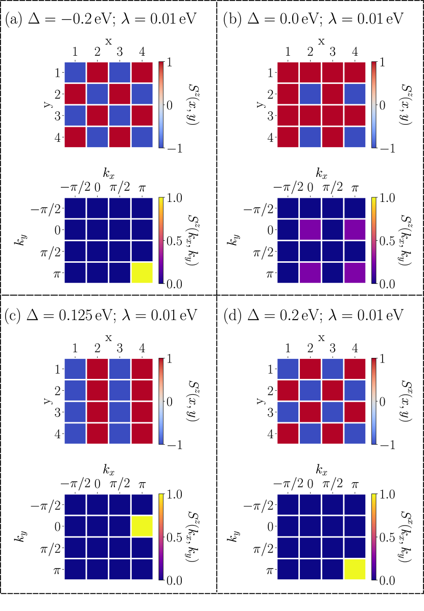
Figure 7: Spin components $S^{z}$ (a)-(c) and $S^{x}$ (d) per site as well as for all relevant wavevectors $\mathbf{k}$ for a 4$\times$4 square lattice. Calculations were performed with semiclassic parallel tempering MC. In (a)-(d) snapshots of the different phases arising in the parameter range $-0.2<\Delta<0.2$ and $0.01\,\text{eV}<\lambda<0.08\,\text{eV}$ are shown. These can be directly compared to the ED results of Fig. 10.

In the regime $-0.12\;\textrm{eV}<\Delta\lesssim 0$, an additional phase is finally seen that has finite SSF’s for several momenta: $(\pi,0)$, $(\pi,\pi)$, and $(0,0)$. To clarify the nature of this phase, we performed MC simulations on a $4\times 4$ cluster, where we include weak SOC $\lambda=0.01\,\text{eV}$ for numerical reasons. In Fig. 7 (a)-(d), snapshots of the four phases appearing in the MC results are shown for the whole $\Delta$ range discussed above. For $\Delta=0$ the pattern becomes an alternation of AFM and FM stripes [Fig. 7 (b)], which leads to maxima at $S^{z}(\pi,0),S^{z}(0,\pi),S^{z}(\pi,\pi)$, and $S^{z}(0,0)$ in the momentum space comparable to the signatures in the SSF of the ED. This phase is from here on referred as “3-up-1-down”.

Overall, the phases seen in the semiclassical model are in good agreement with the characterization based on ED results. For $\Delta=-0.2\;\textrm{eV}$ [Fig. 7 (a)], the out-of-plane checkerboard AFM pattern is the ground state with a maximum at $S^{z}(\pi,\pi)$ and a clear checkerboard pattern in $z$-direction in position space. After the novel “3-up-1-down” phase at $\Delta\approx 0$, positive $\Delta\approx 0.125\,\text{eV}$ leads to a stripy pattern with a maximum at $S^{z}(\pi,0)$ [Fig. 7 (c)] and larger $\Delta=0.2\,\text{eV}$ to the in-plane AFM order with maxima at $S^{x}(\pi,\pi)$ and $S^{y}(\pi,\pi)$, both in accordance with the ED results. Reference [28], which restricts itself to FM and Néel AFM phases, reports an FM phase with some AFM correlations at weak CF,i.e., also sees competition of FM and AFM tendencies roughly where we find the stripy and “3-up-1-down” patterns.

III.2 Phase diagram of the full spin-orbital model

After discussing the limiting cases of small and large CF and SOC, we now investigate the $\Delta$-$\lambda$ plane. We first study the static SSF for fixed $\lambda$ and $\Delta$ [Fig. 6 (a)-(d)]. Since we perform ED on an eight site cluster, the SSF is only obtainable for eight different $\mathbf{k}$ values, from which only four are unique. These are $\mathbf{k}=(0,0)$ resp. FM ordering, $(\pi,0)$ resp. stripy ordering, $(\pi,\pi)$ resp. AFM ordering and $(\pi/2,\pi/2)$. In Fig. 6 (a)-(d) only the SSF’s with appreciable weight are displayed. Our goal is an understanding of the impact of $\lambda$ and $\Delta$ on the spin-orbital state. Hopping parameters $t_{xy}$ , $t_{yz}$, $t_{zx}$, Coulomb repulsion $U$, and Hund’s coupling $J_{H}$ where chosen as introduced in Sec. II.1.

In Fig. 6 (a), CF is fixed to $\Delta=0\,\text{eV}$ and one sees three phases depending on the strength of SOC. For small SOC ($\lambda<0.02\,\text{eV}$), one finds the stripy phase, where $(\pi,0)$-SSF’s have similar in-plane and out-of-plane components. This is in concordance with the results of VCA calculations of [26] as well as ED calculations on a $2\times 2$ cluster [40, 42].

Increasing the SOC to $0.02\,\text{eV}<\lambda<0.04\,\text{eV}$ gives rise to a phase with contributions from in- and out-of-plane ($\pi,0$) as well as ($\pi,\pi$) structure factors and additionally the (0,0) out-of-plane contribution. This phase is the “3-up-1-down” state already discussed in the limit $\lambda=0$ (see Sec. III.1). Increasing SOC further ($\lambda>0.04\,\text{eV}$) leads to an out-of-plane AFM phase. This phase is identical with the out-of-plane AFM phase arising in the triplon model (orange phase in Fig. 5). This phase was also found at $\Delta=0\,\text{eV}$ and substantial SOC in the VCA calculations of [26]. Further increase of SOC starts to reduce the SSF at $(\pi,\pi)$ again, and finally suppresses all AFM order, see the discussion of the triplon model and Fig. 5.

The results for a large fixed CF at $\Delta=0.25\,\text{eV}$ are displayed in Fig. 6 (b). Starting from SOC $\lambda=0\,\text{eV}$, the ground state is an isotropic AFM phase. SOC induces a smooth transition to an in-plane AFM order. This is due to the fact that positive $\Delta$ favors the double occupancy of the $xy$-orbital and therefore $L^{z}=0$, and as $\lambda$ couples spin and orbital momenta, this also leads to a decrease of the $S^{z}$ component.

Lastly in Fig. 6 (d) SOC is set to the value $\lambda=0.06\,\text{eV}$. As already mentioned earlier $\Delta>0.04\,\text{eV}$ stabilizes an in-plane AFM pattern, due to the preference of $L^{z}=0$ which results in a preference of $S^{z}=0$ due to SOC. If the CF is small or has a negative sign, out-of-plane AFM ordering is favored since the $xy$ orbital is mostly singly occupied. This transition is well captured by the triplon model discussed in Sec. III.1.

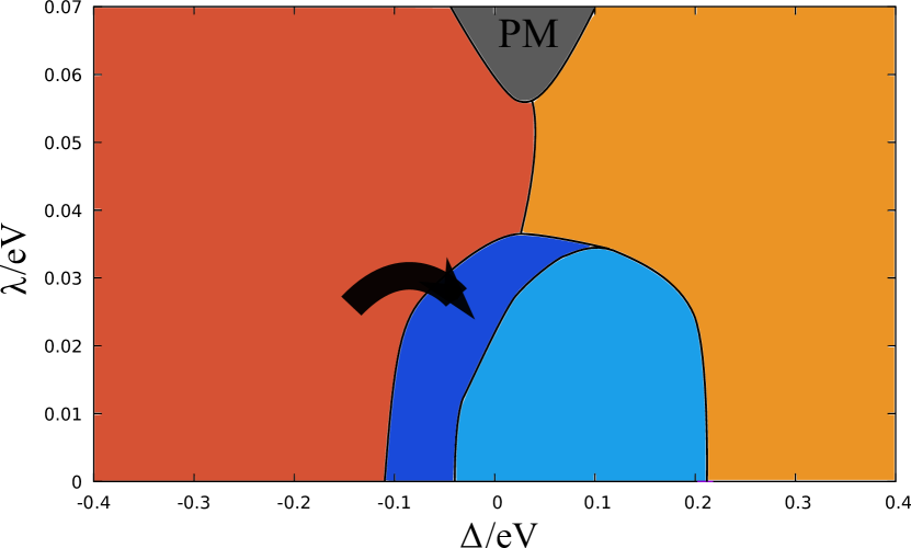
Figure 8: $\Delta-\lambda$ phase diagram obtained by ED calculations on $\sqrt{8}\times\sqrt{8}$ cluster. The PM phase (dark grey) was identified via the triplon model of Sec. II.2. Sketches show the spin ordering for the respective phase, calculated via MC on a $4\times 4$ cluster. The white dots denote the snapshots of the taken in Fig. 10, to investigate the dynamical SSF (further information see Sec. III.4), including the parameter setting for $\text{Ca}_{2}\text{RuO}_{4}$. calculations.

The information gained from the ED SSF’s, supported by semiclassical MC in case of the “3-up-1-down” pattern, as well as the information on the transition to the PM phase inferred from the triplon model is summarized in the $\Delta-\lambda$ phase diagram in Fig. 8. To obtain this phase diagram we performed multiple sweeps by varying $\Delta$ for fixed $\lambda$ (and vice versa), like in Fig. 6, and included the PM phase from the triplon model. We did this because the transition is better identifiable than with $\braket{J^{2}}$ (see Fig. 4). If both CF and SOC are weak, the interaction terms introduced in (II.1)-(II.1) dominate, which favor a stripy alignment of spins (light blue) together with a complex orbital pattern [34, 26]. For large CF, the double occupation locates either at the $xy$ ($\Delta>0$) or alternates between $zx$- and $yz$-orbitals ($\Delta<0$), which results in an $x$-$y$-AFM (light orange) or $z$-AFM order (dark orange) respectively. These phases are both very robust against SOC, which favors a $J=0$ PM phase (dark grey). The competition between the $z$-AFM and the stripy phase at small negative CF and small SOC, causes the “3-up-1-down” phase to arise (dark blue).

Locating $\text{Ca}_{2}\text{RuO}_{4}$ in this phase diagram (corresponding white dot in Fig. 8), puts it solidly within the in-plane AFM phase, as expected from experiment [24, 38, 37, 17]. Also, $\text{Ca}_{2}\text{RuO}_{4}$ does not appear to be very close to any CF-driven phase transition and its AFM order can thus be expected to be rather robust.

III.3 Comparison of semiclassical and quantum models

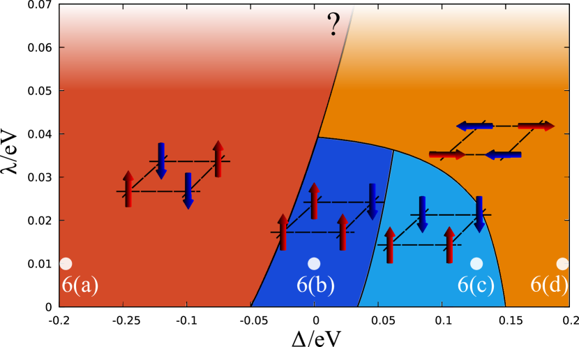
Figure 9: Phase diagram depending on $\lambda$ and $\Delta$ obtained via MC for remaining parameters as given in Sec. II.1. White dots denote the snapshots of Fig. 7.

Having made use of a semiclassical Markov chain MC to identify the “3-up-1-down” phase, we now compare the semiclassical and quantum phase diagrams more generally. Several snapshots for weak SOC were already discussed in Sec. III.1 to clarify the regime of weak SOC and $\Delta\lesssim 0$. To obtain a full semiclassical phase diagram, several CF sweeps for different strengths of SOC between $-0.2\,\text{eV}<\Delta<0.2\,\text{eV}$ were performed and the SSF for $(\pi,\pi)$, $(\pi,0)$ and $(0,0)$ are calculated. The results yield the phase diagram shown in Fig. 9 [white points denote the locations of the snapshots of Fig. 7 (a)-(d)]. For dominant SOC $\lambda>0.04\,\text{eV}$ and $\Delta<0$, an out-of-plane AFM phase arises (dark orange in Fig. 9), while positive CF $\Delta>0\,\text{eV}$ gives rise to an in-plane AFM phase (light orange). For strong CF $|\Delta|>0$ both phases stay stable up to $\lambda=0$. For weak SOC $\lambda<0.04\,\text{eV}$ and CF $0.05\,\text{eV}<\Delta<0.15\,\text{eV}$, the interaction part in the Hamiltonian becomes dominant. This is similar to Sec. III.2, which leads to an out-of-plane stripy phase (light blue). The competition between the stripy and the out-of-plane AFM phase leads to the “3-up-1-down” phase (dark blue) already discussed in Sec. III.1 at $-0.05\,\text{eV}<\Delta<0.05\,\text{eV}$ for $\lambda<0.04\,\text{eV}$.

This phase diagram is in good qualitative agreement with the spin-orbit model (Fig. 5). The exact location of the phase transitions differ somewhat between semiclassical and quantum models. In comparison to the ED simulations, in the semiclassical calculations the AFM phases (both in- and out-of-plane) are more dominant. While ED predicts the $z$-AFM phase to end at $\Delta\approx-0.1\,\text{eV}$ for $\lambda=0\,\text{eV}$, in the semiclassical simulations the $z$-AFM phase stays robust until $\Delta\approx-0.05\,\text{eV}$ (same for the $x-y$-AFM ordering see Fig. 8 and Fig. 9). While the origin for the the difference might lie in the small clusters used (especially for ED), it is quite plausible that quantum fluctuations have the strongest impact near orbital degeneracy. The fact that semiclassical MC captures the same phases as ED, gives a promising pathway that effective spin-orbital models can also be studied on significant larger cluster size with semiclassical MC while still giving reasonable results.

III.4 Dynamic spin-structure factor

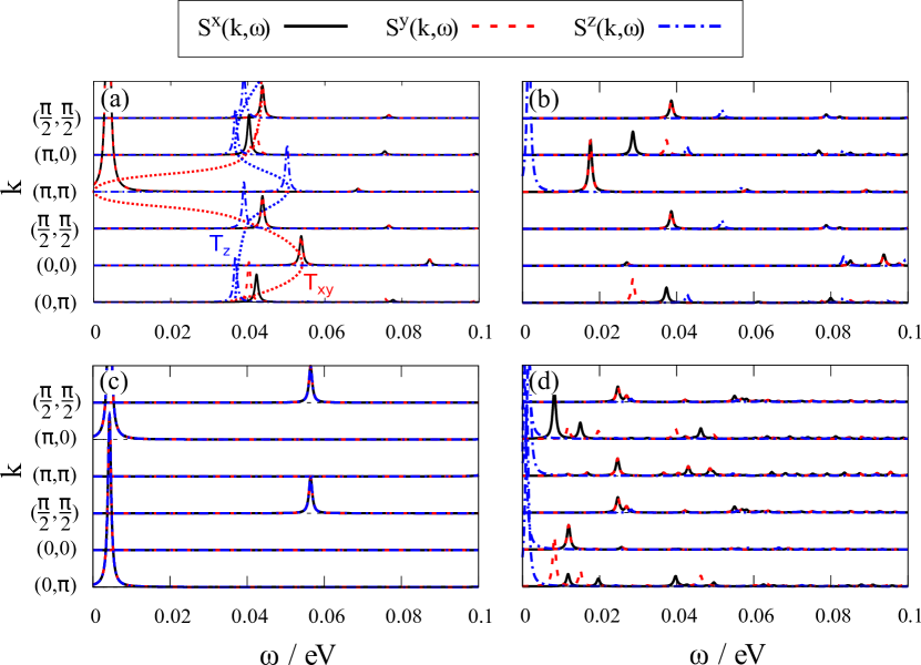
Figure 10: Dynamical spin structure factor $S(\mathbf{k},\omega)$ for (a) $\Delta=0.25\,\text{eV};\lambda=0.065\,\text{eV}$, (b) $\Delta=0.0\,\text{eV};\lambda=0.06\,\text{eV}$, (c) $\Delta=0.15\,\text{eV};\lambda=0\,\text{eV}$, and (d) $\Delta=0.0\,\text{eV};\lambda=0.03\,\text{eV}$. Parameters in (a) are the ones used to describe $\text{Ca}_{2}\text{RuO}_{4}$ [26] and capture the characteristics of INS experiments.

Experimentally, the various phases might be distinguished via magnetic excitations. Therefore we discuss here the signatures expected for the dynamic spin-structure factor

$$S^{\alpha}(\mathbf{k},\omega)=-\frac{1}{\pi}\text{Im}\bra{\phi_{0}}S^{\alpha}(-\mathbf{k})\frac{1}{\omega-H+i0^{+}}S^{\alpha}(\mathbf{k})\ket{\phi_{0}},$$ (12)

which gives an $\omega$ resolution of the phases introduced in Fig. 6. This can then be compared to inelastic neutron scattering [24, 17]. In Fig. 10 the DSSF’s of the four distinct phases are shown. The locations of these snapshots in the phase diagram are denoted with white dots in Fig.8.

III.4.1 Excitations of the in-plane AFM regime

For $\Delta=0.25\,\text{eV}$ and $\lambda=0.065\,\text{eV}$ [Fig. 10 (a)], the the Goldstone mode at $(\pi,\pi)$ allows us to identify the in-plane AFM phase found above in Fig. 6 (b) and (d). The spectrum of Fig. 10(a) was already presented in Ref. [26] as the parameters closely fit Ca₂RuO₄. As already discussed in [26] the in-plane (red guideline) and out-of-plane (blue guideline) transverse modes can be identified. Especially the in-plane transverse mode shows an excellent agreement to [17] reproducing the maximum at $\mathbf{k}=(0,0)$ and $\omega=0.54\,\text{eV}$.

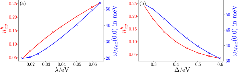
Figure 11: Excitation energy $\omega_{\textrm{max}}$ at $\mathbf{k}=(0,0)$ (blue) and hole density $n^{h}_{xy}$ in the $xy$ orbital (red). (a) Depending on SOC for CF $\Delta=0.25\,\text{eV}$ and (b) depending on CF for SOC $\lambda=0.065\,\text{eV}$.

This maximum, a characteristic signature of the $x$-$y$ symmetry of the magnetic moments, strongly depends on the hole density $n^{h}_{xy}$ in the $xy$-orbital, which is $n^{h}_{xy}\approx 0.25$ in Fig. 10(a). Figure 11(a) shows the dependence of $n^{h}_{xy}$ and of the excitation energy $\omega_{\text{Max}}(0,0)$ on SOC $\lambda$. The excitation energy at $\mathbf{k}=(0,0)$ increases steadily from a minimum at $\omega\approx 0.02\,\text{eV}$ to the maximum $\omega=0.54\,\text{eV}$ for the $\text{Ca}_{2}\text{RuO}_{4}$ parameters in Fig. 10 (a). Having a maximum at $\mathbf{k}=(0,0)$ is thus closely connected to finite - but not necessarily large - hole density in the $xy$-orbital.

Without SOC, strong CF $\Delta=0.25\,\text{eV}$ localizes the two holes in the $zx$- and $yz$-orbital, with $n_{xy}^{h}\approx 0.05$, in agreement with ab-initio calculations for Ca₂RuO₄ performed without SOC [43, 44]. Increasing SOC softens this polarization because it couples $\mathbf{S}$ and $\mathbf{L}$ and thus competes with $\Delta$. SOC increases the hole density at $xy$ so that it reaches $n_{xy}^{h}=0.25$ at $\lambda=0.065\,$eV. On one hand, this implies that the $xy$-orbital continues to be rather close to fully occupied and justifies the picture of Ca₂RuO₄ as orbitally ordered [25]. On the other hand, Figs. 11(a) and 10(a) reveal that the relatively few holes in the $xy$-orbital have a decisive impact on magnetic excitations.

Vice versa, if SOC is fixed and the CF is increased [Fig. 11 (b)] the maximum at $\mathbf{k}=(0,0)$ vanishes. Starting at $\lambda=0.065\,$eV and $\Delta=0.25\,$eV the maximum is, as already discussed, at $\omega=54\,$meV. Increasing $\Delta$ up to $\Delta=0.6\,$eV strongly suppresses the hole density in the $xy$-orbital and at the same time leads to a minimum in the excitation spectrum at $\mathbf{k}=(0,0)$ and $\omega=36\,$meV. It is of note that while the hole density appears to be linked to $\omega$ at $\mathbf{k}=(0,0)$, it is not the only influence. This can be concluded by the fact that for the parameter settings $\Delta=0.25\,\text{eV};\,\lambda=0.015\,\text{eV}$ and $\Delta=0.6\,\text{eV};\,\lambda=0.065\,\text{eV}$ the hole densities are very similar ($n_{xy}^{h}\approx 0.05$) while $\omega_{\text{Max}}(0,0)$ of the excitation differs by a factor of $1.8$ between strong and weak values of SOC and CF. This means that SOC and CF also have direct influence to the excitation at $\mathbf{k}=(0,0)$ in addition to the indirect influence via the hole density of $n_{xy}^{h}$.

Taken together, the extensive study of the excitation at $\mathbf{k}=(0,0)$ has shown that excitation spectra already differ from the one measured in [17] for relatively weak changes in $\lambda$ and $\Delta$, even though the ground state of $\text{Ca}_{2}\text{RuO}_{4}$ is quite robust against such perturbations. It is therefore remarkable that the DSSF in Fig. 10(a) of the effective model is in such close agreement with the experimental data.

III.4.2 Excitations of the PM and various out-of-plane AFM phases

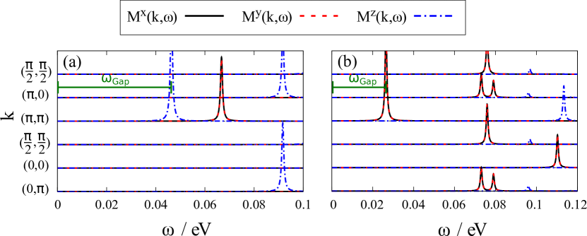
Figure 12: Dynamical magnetic structure factor $\mathbf{M}(\mathbf{k},\omega)$ for (a) $\Delta=0.0\,$eV and (b) $\Delta=0.25\,$eV with substantial SOC $\lambda=0.12\,$eV. $\omega_{\text{Gap}}$ marks the energy gap between the ground state and the lowest lying excitation.

Decreasing CF to $\Delta=0.0\,\text{eV}$ and leaving $\lambda=0.06\,\text{eV}$, the lowest excitation only has out-of-plane contributions [Fig. 10(b)]. This indicates $z$-AFM ordering, cf. Fig. 6 (a) and (d), although the system is here close to the PM state, see Fig. 8. Choosing a large value for SOC $\lambda=0.12\,\text{eV}$ firmly puts the system into the PM state, and the excitation minimum at $(\pi,\pi)$ moves to higher $\omega$. This can be seen in Fig. 12(a), with the magnetization $\mathbf{M}=2\mathbf{S}-\mathbf{L}$ and the dynamical magnetic structure factor obtained analogue to (12). The excitation gap is $\omega_{\text{Gap}}=0.046\,\text{eV}$ [Fig. 12(a)] meaning there is a significant energy cost for the system to create a triplon.

Increasing the CF to $\Delta=0.25\,\text{eV}$ [Fig. 12 (b)] one can see that (i) the lowest-energy triplon has now $x$-$y$ character and (ii) its energy is decreased significantly to $\omega_{\text{Gap}}=0.027\,\text{eV}$. The finite CF thus reduces triplon energy so that they can eventually condense into magnetic order. This can also be seen nicely in Fig. 8 where $\text{Ca}_{2}\text{RuO}_{4}$ (corresponding white dot in Fig. 8) would be in the PM phase if it had no significant CF splitting.

Spectra for the stripy and and “3-up-1-down” phases realized near orbital degeneracy are shown in Fig. 10 (c) resp. (d). The stripy phase ($\Delta=0.15\,\text{eV};\lambda=0\,\text{eV}$) in Fig. 10 (c) not only shows spin isotropy but also a degeneracy between $x$- ($\pi,0$) and $y$-stripy ($0,\pi$) order. Finally, the DSSF of the “3-up-1-down” phase from Fig. 6 (a) is displayed in Fig. 10 (d) and shows the many ordering vectors contributing for $\omega\to 0$.

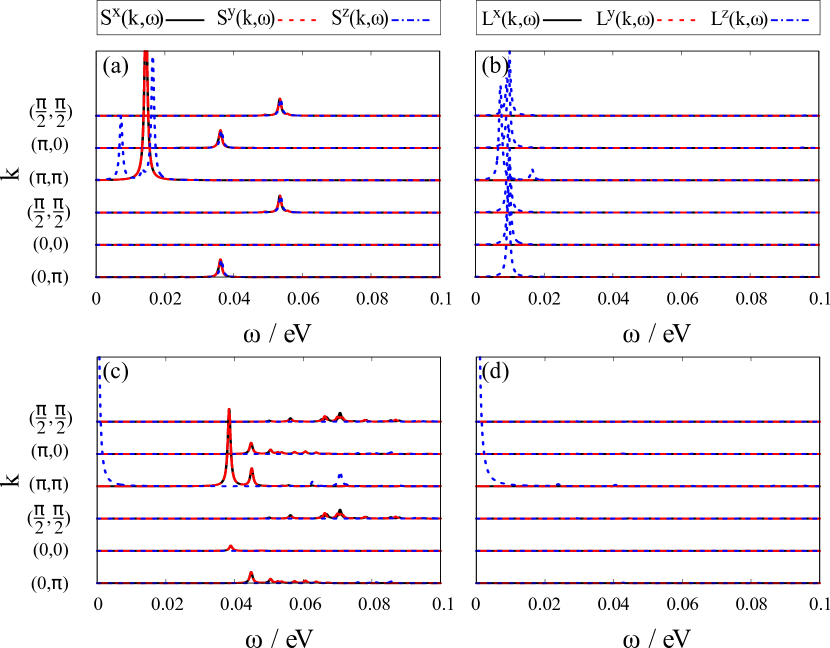
Figure 13: Dynamical Spin and Orbital structure factors for crystal field $\Delta=-0.3\;\textrm{eV}$ and weak SOC. (a) and (c) show the DSSF (12) while (b) and (d) give the orbital analogue based on (II.1). In (a) and (b), $\lambda=0.002\;\textrm{eV}$ and in (c) and (d), $\lambda=0.01\;\textrm{eV}$.

The last phase to be discussed in detail is the checkerboard AFM order with out-of-plane anisotropy at $\Delta\lesssim 0$. For $\lambda=0$, moderate CF $\Delta\approx-0.3\;\textrm{eV}$ is enough to fix the $xy$ orbital to half filling, so that either $xz$ or $yz$ orbitals are double occupied. These two states alternate in a checkerboard pattern with the same unit cell as a Heisenberg-symmetric AFM. A corresponding magnetic excitation spectrum is shown in Fig. 13(a), where weak $\lambda=0.0002\;\textrm{eV}$ induces slight Ising anisotropy into a nearly isotropic spectrum. For the orbital analogue to the DSSF, the spin operator $S^{\alpha}$ in (12) is replaced by angular-momentum operators (II.1). The resulting spectrum shown in Fig. 13(b) is, however, featureless, because alternating order in real orbitals is quadrupolar and would show up in the $(L^{x})^{2}-(L^{y})^{2}\propto n_{xz}-n_{yz}$ channel.

Already for rather small $\lambda=0.01\;\textrm{eV}$, however, Ising anisotropy in spin excitations is very pronounced with an ordered moment along $z$ and a substantial excitation gap, see Fig. 13(c). At the same time, orbital order is now also clearly dipolar and peaked at $(\pi,\pi)$, see Fig. 13(d). SOC has thus coupled spin and orbital ordering into a checkerboard pattern with $L^{z}=1$, $S^{z}=-1$ in one sublattice and $L^{z}=-1$, $S^{z}=1$ on the other. In contrast to $\Delta>0$ discussed above, where SOC induces a gradual crossover from a Heisenberg spin-one system to an excitonic AFM state, the transition between the isotropic and Ising states is here much more abrupt.

IV Discussion and Conclusions

In this paper we investigate an effective low-energy spin-orbital Hamiltonian for spin-orbit coupled Mott insulators like $\text{Ca}_{2}\text{RuO}_{4}$. This model interpolates from the strong-SOC regime, where a description in terms of triplons is applicable, to vanishing SOC and moreover includes Hund’s coupling and anisotropic hopping. For this model, we performed ED calculations on a $\sqrt{8}\times\sqrt{8}$ square lattice to obtain both static and dynamic SSF’s for varying CF $\Delta$ and SOC $\lambda$. The results for the static SSF indicated the existence of four distinct phases. Namely a $z$-AFM and $xy$-AFM with checkerboard pattern, stripy-AFM and a “3-up-1-down” phase at small CF and SOC $\lambda\gtrsim 0$. The stripy and “3-up-1-down” arise near orbital degeneracy, i.e., when neither SOC nor CF dominate, out of the competition and partial frustration of various superexchange terms. The two checkerboard phases, in contrast, extend to large CF’s and include excitonic variants at moderate SOC, whereas strong SOC finally drives a transition to a PM state.

We supplemented the ED analysis of the full quantum model with MC calculations for a semiclassical variant of the same spin-orbital model on a $4\times 4$ cluster. Overall agreement between the semiclassical and quantum-mechanical models was quite good, with the largest differences found around orbital degeneracy $\Delta,\lambda\approx 0$. The transition to the PM $J=0$ phase at strong SOC coupling was clarified with the help of an effective triplon model comparable to [14]. Combining these results gave us a complete $\Delta-\lambda$ phase diagram that establishes the competition of CF and SOC for strongly correlated $t_{2g}^{4}$ systems.

We also investigate the DSSF and show that there is a remarkable correspondence [26] between calculations based on ab initio parameters and neutron-scattering results, despite the fact that the calculations appear to strongly depend on the hole density in the $xy$-orbital. Parameter dependence is also quite sensitive, which makes this a stringent test of the model that allows a distinction between orbital degeneracy lifted by a CF or by SOC. We further give spectra expected for the other phases found with the model.

In contrast to the gradual impact of SOC on the excitations of the orbitally polarized regime $\Delta>0$, a much clearer transition is revealed at $\Delta<0$. Relatively small SOC is enough to switch from alternating orbital order and Heisenberg AFM to order involving complex orbitals. However, coupling to further lattice distortions, not discussed here, would be expected to push this transition to stronger SOC. This physics might also be relevant to $t_{2g}^{2}$ systems, i.e., with two electrons as in vanadates, where similar alternating or orbital order arises [41]. Although SOC for two electrons has opposite sign than the two-hole case discussed here, this does not qualitatively affect results in the parameter regime with effective Ising symmetry, i.e. when $\Delta<0$ leads to nearly empty (for $t_{2g}^{2}$) resp. always doubly occupied (for $t_{2g}^{4}$) $xy$ orbitals. The spin-orbital superexchange model discussed here can naturally be extended to the two-electron case also beyond this regime.