Homogenization Theory of Ion Transportation in Multicellular Tissue

Abstract

Ion transport in biological tissues is crucial in the study of many biological and pathological problems. Some multi-cellular structures, like smooth muscles on the vessel walls, could be treated as periodic bi-domain structures, which consist of intracellular space and extracellular space with semipermeable membranes in between. With the aid of two-scale homogenization theory, macro-scale models are proposed based on an electro-neutral (EN) microscale model with nonlinear interface conditions, where membranes are treated as combinations of capacitors and resistors. The connectivity of intracellular space is also taken into consideration. If the intracellular space is fully connected and forms a syncytium, then the macroscale model is a bidomain nonlinear coupled partial differential equations system. Otherwise, when the intracellular cells are not connected, the macroscale model for intracellular space is an ordinary differential system with source/sink terms from the connected extracellular space.

Keywords: Ion transport, Two-scale homogenization, Bi-domain model, Connectivity

Introduction

Ions in human body play vital roles in many aspects such as helping the transport of nerve impulses, maintaining the proper functions of muscles, activating various enzymes, helping blood coagulation and so on. Studying ion transport in biological tissues can help us understand the mechanisms of many physiological phenomenon and gain some insight about how to treat certain diseases. The Poisson-Nernst-Planck (PNP) system is one of the most popular mathematical models that describe the ion transport under the influence of both ionic concentration gradient and electric field. PNP system has extensive and successful applications in biological systems, particularly in ion channels on cell membrane [10, 12, 17, 24, 27, 37]. Due to the capacitance of membranes, there are thin boundary layers (BLs) near the interfaces formed by excessive charges accumulation. BLs requires extra computation cost during numerical simulations in order to resolve the fast change behaviors of solution inside the layers and attain certain accuracy [8, 44]. A lot of efforts are put in order to get rid of this constrain, like Mori [33]. By using asymptotic analysis, Song et al. [43, 42] proposed effective interface conditions by introducing a time dependent capacitance on the membrane. In this paper, we take the linearization of the effective boundary conditions and propose a microscale EN PNP system with interface conditions describing the membrane fluxes and capacitor effect.

Due to the existence of pumps on membranes, ion concentrations across the membrane are discontinuous, for example potassium is $140\sim 150~{}mM$ in the intracelluar space and $3\sim 5~{}mM$ in the extracellular space. However, the flux across the membrane is continuous and determined by conductance and the difference between membrane potential and Nernst Potential. When studying biological tissues, there are thousands of cells in the system and the solution is highly oscillatory. The obtained mircoscale model requires significant computational resources to solve numerically. In order to simulate ion transport in biological tissues more efficiently, an effective macroscale model is demanded. One of the most popular ways to derive the macroscale models is through homogenization by deriving an “average” or ”effective” homogenized system, which extracts macro information from micro structures. Specific methods of homogenization include oscillating test function method [45], asymptotic expansion method [6], two-scale method [36, 1] and unfolding method [15, 13]. The homogenization theory for system with jump solution is first developed by Monsurro and Donato [30, 32, 21, 18] to a linear elliptic model for heat conductors problem by using extension operators. Results for linear parabolic and hyperbolic equations can be found in [28, 20, 48, 47, 19]. Another factor for bi-domain homogenization is whether two sub-domains are all connected domain, respectively. The linear problems mentioned above only considered the case when one sub-domain is embedded in the other sub-domain and disconnected. In [9], a linear diffusion problem in a bi-domain with flux jump at the interface is discussed. The authors considered both when one sub-domain is connected and disconnected, and explained the reasons for the difference in the resulting homogenization systems for the two cases, which is mainly due to the different spaces of the test functions. For nonlinear bi-domain homogenization problems, the main difficulty is the strong convergence requirement both in domain and on the interface. By two-scale convergence and unfolding operator, Gahn et al. [25, 23] proposed homogenization results for a nonlinear problem in a bi-domain for calcium dynamics (connected sub-domains) and diffusion-reaction system (one disconnected sub-domain).

For the homogenization theory of PNP system, which is a nonlinear coupled system, asymptotic expansion method [29] is first used to derive the homogenized system for the linearized Navier-Stokes-PNP model in porous media in [38]. Later, a rigorous derivation by using two-scale method is proposed by Alliare et al. [4]. Similar method is extended to study ion transport through deformable porous media [2]. Homogenization of a full nonlinear PNP model in porous media is discussed in [46, 41] by using unfolding method and two-scale method, where nonflux boundary condition is used on the interface for ion concentraion. Most of the homogenization research for PNP model and ion transport model are established in porous media without considering the electric-diffusion of ions in the intracellular region, and sometimes linearization technique is used to simplify the process. In this paper, by using unfolding operator and two-scale convergence, we develop the homogenization theory for the fully nonlinear EN bi-domain model in the whole domain with nonlinear interface flux boundary conditions which depends on the jumps of ion concentrations, electric potential, and the time derivative of potential jump. Two different scenarios, connected and disconnected intracellular regions, are both taken into consideration and lead to different macroscopic models.

The remainder of this paper is organized as follows: The microscale EN ion transport model is given in Section 2; Section 3 is devoted to proving the a priori estimates; Then convergence results and homogenization process are presented in Section 4 according to different connectivity conditions of intracellular region; we draw conclusions in the last section.

Setting of the mathematical model

In this section, a microscale EN bi-domain ion transport model in multicellular tissues is introduced. Consider a domain $\Omega=(0,1)^{d}$ which consists of two components: $\Omega_{I}^{\varepsilon}$ and $\Omega_{E}^{\varepsilon}$ (see Figure 1). Let $Y=(0,1)^{d}$ and $Y_{I},Y_{E}$ are two disjoint subsets of $Y$, such that

$$\overline{Y}=\overline{Y_{E}}\cup\overline{Y_{I}}.$$

And $\Gamma=\partial Y_{I}\bigcap\partial Y_{E}$ is Lipschitz continuous. Let $\vec{n}_{1}$ be the normal direction of $\Gamma$, pointing from $Y_{I}$ to $Y_{E}$. Let $\beta_{s},s=I,E$ be the characteristic function on $Y_{s},s=I,E$, which extend periodically to $\mathbb{R}^{d}$. For any $k\in\mathbb{Z}^{d}$, let

$$Y^{k}=k+Y,~{}\Gamma^{k}=k+\Gamma,~{}Y_{s}^{k}=k+Y_{s},$$

where $k=\left(k_{1},\cdots,k_{d}\right)$, $s=I,E$. For any $\varepsilon>0$ and $1/\varepsilon\in\mathbb{N}^{+}$, let $K_{\varepsilon}=\left\{k\in\mathbb{Z}^{d}|\varepsilon Y_{s}^{k}\cap\Omega\neq\emptyset,s=I,E\right\}$. Denote the two disjoint subsets of $\Omega$ and the interface between them as:

$$\Omega_{I}^{\varepsilon}=\bigcup_{k\in K_{\varepsilon}}\varepsilon Y_{I}^{k},\quad\Omega_{E}^{\varepsilon}=\Omega\backslash\overline{\Omega_{I}^{\varepsilon}},\quad\Gamma_{\varepsilon}=\bigcup_{k\in K_{\varepsilon}}\varepsilon\Gamma^{k}.$$

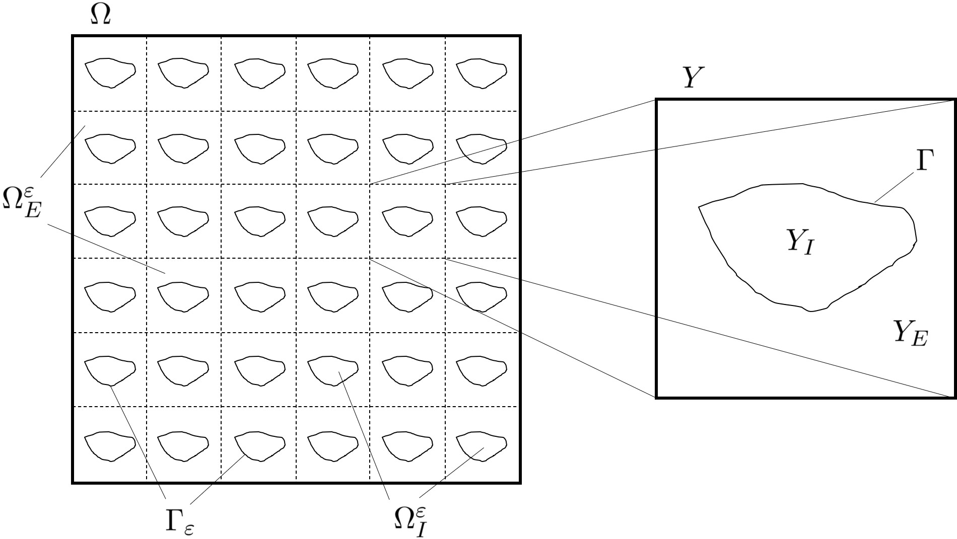
Figure 1: Schematic of the domain $\Omega$.

So $\Omega=\Omega_{I}^{\varepsilon}\bigcup\Omega_{E}^{\varepsilon}\bigcup\Gamma_{\varepsilon}$ and $\Omega$ is a union of $\varepsilon Y$-periodic sets. Assume both $\Omega_{E}^{\varepsilon}$ and $\Omega_{I}^{\varepsilon}$ have Lipschitz boundaries, especially $\Gamma_{\varepsilon}$ is a Lipschitz boundary.

Consider three different ion species in $\Omega$: $\mathrm{Na^{+},K^{+},Cl^{-}}$, their concentrations and valences are denoted by $C_{i,s}^{\varepsilon},i=1,2,3,s=I,E$ and $z_{i}$ respectively, the electric potential is $\phi_{s}^{\varepsilon}$, subscript $s$ represent variables in $\Omega_{s}^{\varepsilon},s=I,E$.

The assumptions are summarized as follows:

• Connectivity: $\Omega_{E}^{\varepsilon}$ is connected and $\Omega_{I}^{\varepsilon}$ can be connected or not (see Figure 1).

• Positivity:

  $$0<C_{d}\leq C_{i,s}^{\varepsilon}\leq C_{u}~{}~{}~{}~{}\text{on}~{}\Gamma_{\varepsilon},~{}~{}i=1,2,3,s=I,E,$$ (2.1)

  $$0<C_{l}<\sum\limits_{i=1}^{3}z_{i}^{2}C_{i,s}^{\varepsilon}(t,x)~{}~{}~{}~{}\text{in}~{}\Omega_{s}^{\varepsilon},~{}~{}s=I,E,$$ (2.2)

  where $C_{d},C_{u},C_{l}$ are positive constants.

• Electric Neutrality (EN):

  $$\sum\limits_{i=1}^{3}z_{i}C_{i,s}^{\varepsilon}(t,x)=0,~{}~{}s=I,E.$$ (2.3)

• Diffusion Constant: diffusion constants of ions are the same and denoted by $D$.

When $\Omega_{I}^{\varepsilon}$ is not connected, we call this case “connected-disconnected” case. In this case, $\overline{Y_{I}}\subset Y$ and $\Omega_{I}^{\varepsilon}$ is a disconnected union of $\varepsilon Y$-periodic sets of size $\varepsilon Y_{I}$. When $\Omega_{I}^{\varepsilon}$ is connected, we call this case “connected-connected” case. In this case both $Y_{I}$ and $Y_{E}$ reach $\partial Y$, thus both $\Omega_{I}^{\varepsilon}$ and $\Omega_{E}^{\varepsilon}$ reach $\partial\Omega$.

The EN bi-domain ion transport model is given as follow: for $i=1,2,3,s=I,E$,

$$\partial_{t}C_{i,s}^{\varepsilon}=-\nabla\cdot{J}_{i,s}=\nabla\cdot[D(\nabla C_{i,s}^{\varepsilon}+z_{i}C_{i,s}^{\varepsilon}\nabla\phi_{s}^{\varepsilon})]~{}~{} in~{}(0,T)\times\Omega^{\varepsilon}_{s},$$ (2.4a)

$$z_{i}{J}_{i,s}\cdot\vec{n}=\varepsilon G_{i}\big{(}\llbracket{\phi^{\varepsilon}}\rrbracket+\dfrac{1}{z_{i}}\llbracket{\ln C_{i}^{\varepsilon}}\rrbracket\big{)}+\varepsilon P_{i}^{\varepsilon}+\varepsilon\lambda_{i}P_{m}\partial_{t}\llbracket{\phi^{\varepsilon}}\rrbracket~{}~{} on~{}(0,T)\times\Gamma_{\varepsilon},$$ (2.4b)

$${J}_{i,E}\cdot\vec{\nu}=0~{}~{} on~{}(0,T)\times\partial\Omega,$$ (2.4c)

$$C_{i,s}^{\varepsilon}|_{t=0}=C_{i,s}^{0}~{}~{} in~{}\Omega^{\varepsilon}_{s}.$$ (2.4d)

and

$$-\nabla\cdot(D\sigma_{s}^{\varepsilon}\nabla\phi_{s}^{\varepsilon})=0~{}~{} in~{}(0,T)\times\Omega^{\varepsilon}_{s},$$ (2.5a)

$$-D\sigma_{s}^{\varepsilon}\nabla\phi_{s}^{\varepsilon}\cdot\vec{n}=\sum\limits_{i=1}^{3}\varepsilon G_{i}\llbracket{\phi^{\varepsilon}}\rrbracket+\sum\limits_{i=1}^{3}\varepsilon G_{i}\dfrac{1}{z_{i}}\llbracket{\ln C_{i}^{\varepsilon}}\rrbracket+\varepsilon I_{P}^{\varepsilon}+\varepsilon P_{m}\partial_{t}\llbracket{\phi^{\varepsilon}}\rrbracket~{}~{} on~{}(0,T)\times\Gamma_{\varepsilon},$$ (2.5b)

$$-D\sigma_{E}^{\varepsilon}\nabla\phi_{E}^{\varepsilon}\cdot\vec{\nu}=0~{}~{} on~{}(0,T)\times\partial\Omega,$$ (2.5c)

$$\llbracket{\phi^{\varepsilon}}\rrbracket|_{t=0}=\phi^{0}~{}~{} on~{}\Gamma_{\varepsilon}.$$ (2.5d)

where $\phi_{s}^{\epsilon}$ is the electric potential in domain $\Omega_{s}$, $C_{i,s}^{\epsilon}$ is the concentration of $i_{th}$ ion in domain $\Omega_{s}$.

(2.4a) is the usual Nernst-Planck equation, (2.5) is a direct result of (2.4) and EN assumption (2.3) with

$$\sigma_{s}^{\varepsilon}=\sum\limits_{i=1}^{3}z_{i}^{2}C_{i,s}^{\varepsilon},~{}~{}s=I,E.$$ (2.6)

(2.4b) is the interface flux condition for ion concentration which consists of three parts.

• The first part is the current induced by passive ion channel which is modeled by Ohm’s Law. Here $G_{i}$ is the conductance of $i_{th}$ ion on the membrane, $\llbracket{\phi^{\varepsilon}}\rrbracket=\phi_{I}-\phi_{E}$ is the membrane potential and $E_{i}\triangleq-\frac{1}{z_{i}}\llbracket{\ln C_{i}^{\varepsilon}}\rrbracket=\frac{1}{z_{i}}(\ln C_{i,E}^{\varepsilon}-\ln C_{i,I}^{\varepsilon})$ is the Nernst potential.

• The second part is the current induced by the active pumps on the membrane. Here we only consider the $Na^{+}/K^{+}$ pumps [49].

  $$P_{1}^{\varepsilon}=3I_{p}^{\varepsilon}~{}~{},P_{2}^{\varepsilon}=-2I_{p}^{\varepsilon},~{}~{}P_{3}^{\varepsilon}=0,$$

  with

  $$I_{p}^{\varepsilon} = I_{\max 1}\left(\frac{C_{1,I}^{\varepsilon}}{C_{1,I}^{\varepsilon}+K_{Na1}}\right)^{3}\left(\frac{C_{2,E}^{\varepsilon}}{C_{2,E}^{\varepsilon}+K_{K1}}\right)^{2}$$ (2.7)

  $$+ I_{\max 2}\left(\frac{C_{1,I}^{\varepsilon}}{C_{1,I}^{\varepsilon}+K_{Na2}}\right)^{3}\left(\frac{C_{2,E}^{\varepsilon}}{C_{2,E}^{\varepsilon}+K_{K2}}\right)^{2},$$

  where $I_{max1},I_{max2}$ are maximum $Na^{+}/K^{+}$ pump current density and $K_{K1},K_{K2}$, $K_{Na1}$, $K_{Na2}$ are threshold constants for $I_{p}^{\varepsilon}$.

• The last term is the current induced by the capacitor effect of membrane with capacitance $P_{m}$ . $\lambda_{i}$ reflects the effect of capacitor on the $i_{th}$ ion species and $\sum\limits_{i=1}^{3}\lambda_{i}=1$. Here we take $\lambda_{i}$ as constant [33] which is simplification and linearization version of models in [43, 42].

Remark 2.1.

In (2.4), (2.5) we only consider the case when $\Omega_{I}^{\varepsilon}$ is not connected, and this would not affect the main idea because when $\Omega_{I}^{\varepsilon}$ is also connected and reaches the exterior boundary $\partial\Omega$, we only need to add another exterior boundary condition for the functions in $\Omega_{I}^{\varepsilon}$. And the connectivity condition of $\Omega_{I}^{\varepsilon}$ would not affect the a priori estimates (Theorem 3.1) either.

The homogenization results (Theorem 4.1 and Theorem 4.2) show that the interfacial fluxes become source terms in the homogenized equations, and the connectivity of intracellular region will affect the homogenization results. When the intracellular region is connected, the homogenized one is a diffusion-reaction equation; when cells are isolated with each other, the homogenized equation is a reaction equation. This is consistent with relevant results in [9]. And the EN condition still holds for the homogenized equations both when intracellular region is connected and not connected.

A priori estimate

In order to derive the convergence results, we need a priori estimates for the solutions of (2.4), (2.5). In the rest of the paper, $A$ (with or without subscript) represent a generic positive constant independent of $\varepsilon$ (in different equations, the value of $A$ may be different).

The weak form of (2.4) and (2.5) is: for $i=1,2,3,s=I,E$, find $C_{i,s}^{\varepsilon}\in L^{2}(0,T;~{}H^{1}(\Omega_{s}^{\varepsilon})),~{}\phi_{s}^{\varepsilon}\in L^{2}(0,T;~{}H^{1}(\Omega_{s}^{\varepsilon}))$, such that

$$\int_{\Omega_{s}^{\varepsilon}}\partial_{t}C_{i,s}^{\varepsilon}v_{s}~{}dx+\int_{\Omega_{s}^{\varepsilon}}D\nabla C_{i,s}^{\varepsilon}\nabla v_{s}~{}dx+z_{i}\int_{\Omega_{s}^{\varepsilon}}C_{i,s}^{\varepsilon}D\nabla\phi_{s}^{\varepsilon}\nabla v_{s}~{}dx$$

$$\pm\varepsilon\int_{\Gamma_{\varepsilon}}\big{(}\dfrac{G_{i}}{z_{i}}\llbracket{\phi^{\varepsilon}}\rrbracket v_{s}+\dfrac{G_{i}}{z_{i}^{2}}\llbracket{\ln C_{i}^{\varepsilon}}\rrbracket v_{s}+\dfrac{P_{i}^{\varepsilon}}{z_{i}}v_{s}+\dfrac{\lambda_{i}}{z_{i}}P_{m}\partial_{t}\llbracket{\phi^{\varepsilon}}\rrbracket v_{s}\big{)}~{}dS=0,$$ (3.1a)

$$\int_{\Omega_{s}^{\varepsilon}}\sigma_{s}^{\varepsilon}D\nabla\phi_{s}^{\varepsilon}\nabla\varphi_{s}~{}dx\pm\varepsilon\int_{\Gamma_{\varepsilon}}\big{(}\sum\limits_{k=1}^{3}G_{k}\llbracket{\phi^{\varepsilon}}\rrbracket\varphi_{s}+\sum\limits_{k=1}^{3}\dfrac{G_{k}}{z_{k}}\llbracket{\ln C_{k}^{\varepsilon}}\rrbracket\varphi_{s}+I_{p}^{\varepsilon}\varphi_{s}+P_{m}\partial_{t}\llbracket{\phi^{\varepsilon}}\rrbracket\varphi_{s}\big{)}~{}dS=0,$$ (3.1b)

for $\forall~{}v_{s}\in L^{2}(0,T;~{}H^{1}(\Omega_{s}^{\varepsilon}))$ and $\varphi_{s}\in L^{2}(0,T;~{}H^{1}(\Omega_{s}^{\varepsilon}))$, where “$\pm$” takes “$+$” for $s=I$ and “$-$” for $s=E$. Next we derive a priori estimates for $C_{i,s}^{\varepsilon},\phi_{s}^{\varepsilon},~{}i=1,2,3,s=I,E$.

We also impose the following condition for $\phi_{E}^{\varepsilon}$ to ensure the uniqueness,

$$\int_{\Omega_{E}^{\varepsilon}}\phi_{E}^{\varepsilon}~{}dx=0.$$ (3.2)

In the rest of the paper, for a subset $\omega\in\mathbb{R}^{d}$, we simply denote $\|f\|_{L^{2}(\omega)}$ as $\|f\|_{\omega}$. And for a function $u^{\varepsilon}$ defined both in $\Omega_{I}^{\varepsilon}$ and $\Omega_{E}^{\varepsilon}$, denote $\|u^{\varepsilon}\|^{2}_{\Omega^{\varepsilon}}\triangleq\|u_{I}^{\varepsilon}\|^{2}_{\Omega_{I}^{\varepsilon}}+\|u_{E}^{\varepsilon}\|^{2}_{\Omega_{E}^{\varepsilon}}$. Then a priori estimates are summarized in the following theorem.

Theorem 3.1.

Let $C_{i,s}^{\varepsilon},\phi_{s}^{\varepsilon},i=1,2,3,s=I,E$ be the solutions of (3.1) and suppose assumption (3.2) hold, then the following estimates are valid, for $i=1,2,3,s=I,E$,

$$\|C_{i,s}^{\varepsilon}\|_{L^{\infty}(0,T;L^{2}(\Omega_{s}^{\varepsilon}))}\leq A,$$ (3.3a)

$$\|C_{i,s}^{\varepsilon}\|_{L^{2}(0,T;H^{1}(\Omega_{s}^{\varepsilon}))}\leq A,$$ (3.3b)

$$\sqrt{\varepsilon}\|C_{i,s}^{\varepsilon}\|_{L^{2}(0,T;L^{2}(\Gamma^{\varepsilon}))}\leq A,$$ (3.3c)

$$\|\partial_{t}C^{\varepsilon}_{i,s}\|_{L^{2}(0,T;H^{-1}(\Omega^{\varepsilon}_{s}))}\leq A,$$ (3.3d)

$$\sqrt{\varepsilon}\|\phi^{\varepsilon}\|_{L^{2}(0,T;L^{2}(\Gamma^{\varepsilon}))}\leq A,$$ (3.3e)

$$\|\phi_{s}^{\varepsilon}\|_{L^{2}(0,T;H^{1}(\Omega_{s}^{\varepsilon}))}\leq A.$$ (3.3f)

Proof: If let $v_{s}=C_{i,s}^{\varepsilon},~{}\varphi_{s}=\phi_{s}^{\varepsilon},~{}s=I,E$ in (3.1), we have

$$\sum\limits_{i=1}^{3}\dfrac{1}{2}\partial_{t}\|C_{i}^{\varepsilon}\|^{2}_{\Omega^{\varepsilon}}+\sum\limits_{i=1}^{3}D\|\nabla C_{i}^{\varepsilon}\|^{2}_{\Omega^{\varepsilon}}+\sum\limits_{i=1}^{3}\int_{\Omega^{\varepsilon}}z_{i}C_{i}^{\varepsilon}D\nabla\phi^{\varepsilon}\nabla C_{i}^{\varepsilon}~{}dx+\sum\limits_{i=1}^{3}\int_{\Gamma^{\varepsilon}}\varepsilon\dfrac{P_{i}^{\varepsilon}}{z_{i}}\llbracket{C_{i}^{\varepsilon}}\rrbracket~{}dS$$

$$+\sum\limits_{i=1}^{3}\int_{\Gamma^{\varepsilon}}\varepsilon\dfrac{G_{i}}{z_{i}}\llbracket{\phi^{\varepsilon}}\rrbracket\llbracket{C_{i}^{\varepsilon}}\rrbracket~{}dS+\sum\limits_{i=1}^{3}\int_{\Gamma^{\varepsilon}}\varepsilon\dfrac{G_{i}}{z_{i}^{2}}\llbracket{\ln C_{i}^{\varepsilon}}\rrbracket\llbracket{C_{i}^{\varepsilon}}\rrbracket~{}dS$$

$$+\sum\limits_{i=1}^{3}\int_{\Gamma^{\varepsilon}}\varepsilon\dfrac{\lambda_{i}}{z_{i}}P_{m}\partial_{t}\llbracket{\phi^{\varepsilon}}\rrbracket\llbracket{C_{i}^{\varepsilon}}\rrbracket~{}dS=0,$$ (3.4a)

$$\int_{\Omega^{\varepsilon}}\sigma^{\varepsilon}D\nabla\phi^{\varepsilon}\nabla\phi^{\varepsilon}~{}dx+\sum\limits_{i=1}^{3}\varepsilon G_{i}\|\llbracket{\phi^{\varepsilon}}\rrbracket\|^{2}_{\Gamma^{\varepsilon}}+\varepsilon\dfrac{P_{m}}{2}\partial_{t}\|\llbracket{\phi^{\varepsilon}}\rrbracket\|^{2}_{\Gamma^{\varepsilon}}$$

$$=-\sum\limits_{i=1}^{3}\int_{\Gamma^{\varepsilon}}\varepsilon\dfrac{G_{i}}{z_{i}}\llbracket{\ln C_{i}^{\varepsilon}}\rrbracket\llbracket{\phi^{\varepsilon}}\rrbracket~{}dS-\int_{\Gamma^{\varepsilon}}\varepsilon I_{p}^{\varepsilon}\llbracket{\phi^{\varepsilon}}\rrbracket~{}dS.$$ (3.4b)

From assumption (2.1), we have

$$\begin{cases}\llbracket{\ln C_{i}^{\varepsilon}}\rrbracket\llbracket{C_{i}^{\varepsilon}}\rrbracket=(\ln C_{i,I}^{\varepsilon}-\ln C_{i,E}^{\varepsilon})(C_{i,I}^{\varepsilon}-C_{i,E}^{\varepsilon})=\dfrac{1}{\xi}(C_{i,I}^{\varepsilon}-C_{i,E}^{\varepsilon})^{2}\geq\dfrac{1}{C_{u}}(C_{i,I}^{\varepsilon}-C_{i,E}^{\varepsilon})^{2}\\ |\llbracket{\ln C_{i}^{\varepsilon}}\rrbracket|=|\ln C_{i,I}^{\varepsilon}-\ln C_{i,E}^{\varepsilon}|=|\dfrac{1}{\xi}(C_{i,I}^{\varepsilon}-C_{i,E}^{\varepsilon})|\leq\dfrac{1}{C_{d}}|C_{i,I}^{\varepsilon}-C_{i,E}^{\varepsilon}|,\end{cases}$$ (3.5)

where $\xi$ is between $C_{i,I}^{\varepsilon}$ and $C_{i,E}^{\varepsilon}$. Then let $\varphi_{s}=\frac{\lambda_{i}}{z_{i}}C_{i,s}^{\varepsilon},~{}s=I,E$ in (3.1b), we have

$$\varepsilon\int_{\Gamma^{\varepsilon}}\dfrac{\lambda_{i}}{z_{i}}P_{m}\partial_{t}\llbracket{\phi^{\varepsilon}}\rrbracket\llbracket{C_{i}^{\varepsilon}}\rrbracket~{}dS$$

$$= -\dfrac{\lambda_{i}}{z_{i}}\int_{\Omega^{\varepsilon}}\sigma^{\varepsilon}D\nabla\phi^{\varepsilon}\nabla C_{i}^{\varepsilon}~{}dx-\varepsilon\dfrac{\lambda_{i}}{z_{i}}\int_{\Gamma^{\varepsilon}}\big{(}\sum\limits_{k=1}^{3}G_{k}\llbracket{\phi^{\varepsilon}}\rrbracket\llbracket{C_{i}^{\varepsilon}}\rrbracket+\sum\limits_{k=1}^{3}\dfrac{G_{k}}{z_{k}}\llbracket{\ln C_{k}^{\varepsilon}}\rrbracket\llbracket{C_{i}^{\varepsilon}}\rrbracket+I_{p}^{\varepsilon}\llbracket{C_{i}^{\varepsilon}}\rrbracket\big{)}~{}dS$$

Combining the above equaiton, (3.5), (2.1) and (3.4a) yields

$$\sum\limits_{i=1}^{3}(\partial_{t}\|C_{i}^{\varepsilon}\|^{2}_{\Omega^{\varepsilon}}+\|\nabla C_{i}^{\varepsilon}\|^{2}_{\Omega^{\varepsilon}}+\varepsilon\|\llbracket{C_{i}^{\varepsilon}}\rrbracket\|^{2}_{\Gamma^{\varepsilon}})$$ (3.6)

$$\leq A_{1}\left(K_{1}\|\nabla\phi^{\varepsilon}\|^{2}_{\Omega^{\varepsilon}}+\dfrac{1}{K_{1}}\sum\limits_{i=1}^{3}\|\nabla C_{i}^{\varepsilon}\|^{2}_{\Omega^{\varepsilon}}\right)+A_{2}\varepsilon\|\llbracket{\phi^{\varepsilon}}\rrbracket\|^{2}_{\Gamma^{\varepsilon}}+A_{3}\varepsilon\sum\limits_{i=1}^{3}\|\llbracket{C_{i}^{\varepsilon}}\rrbracket\|^{2}_{\Gamma^{\varepsilon}}+A_{4}.$$

where we used the fact that $I_{P}^{\varepsilon}$ is bounded.

From assumption (2.2), we can multiply (3.4b) with $\frac{2A_{1}K_{1}}{DC_{l}}$ and add it to (3.6) to get

$$\sum\limits_{i=1}^{3}(\partial_{t}\|C_{i}^{\varepsilon}\|^{2}_{\Omega^{\varepsilon}}+\|\nabla C_{i}^{\varepsilon}\|^{2}_{\Omega^{\varepsilon}}+\varepsilon\|\llbracket{C_{i}^{\varepsilon}}\rrbracket\|^{2}_{\Gamma^{\varepsilon}})+A_{1}K_{1}\|\nabla\phi^{\varepsilon}\|^{2}_{\Omega^{\varepsilon}}+A_{2}\varepsilon\|\llbracket{\phi^{\varepsilon}}\rrbracket\|^{2}_{\Gamma^{\varepsilon}}+A_{3}\varepsilon\partial_{t}\|\llbracket{\phi^{\varepsilon}}\rrbracket\|^{2}_{\Gamma^{\varepsilon}}$$

$$\leq \dfrac{A_{4}}{K_{1}}\sum\limits_{i=1}^{3}\|\nabla C_{i}^{\varepsilon}\|^{2}_{\Omega^{\varepsilon}}+A_{5}\varepsilon\|\llbracket{\phi^{\varepsilon}}\rrbracket\|^{2}_{\Gamma^{\varepsilon}}+A_{6}\varepsilon\sum\limits_{i=1}^{3}\|\llbracket{C_{i}^{\varepsilon}}\rrbracket\|^{2}_{\Gamma^{\varepsilon}}+A_{7}$$

$$\leq \dfrac{A_{4}}{K_{1}}\sum\limits_{i=1}^{3}\|\nabla C_{i}^{\varepsilon}\|^{2}_{\Omega^{\varepsilon}}+A_{5}\varepsilon\|\llbracket{\phi^{\varepsilon}}\rrbracket\|^{2}_{\Gamma^{\varepsilon}}+A_{8}\varepsilon\sum\limits_{i=1}^{3}\left(\varepsilon^{-1}K_{2}\|C_{i}^{\varepsilon}\|^{2}_{\Omega^{\varepsilon}}+\dfrac{1}{K_{2}}\varepsilon\|\nabla C_{i}^{\varepsilon}\|^{2}_{\Omega^{\varepsilon}}\right)+A_{7},$$

where $K_{1},K_{2}$ are two positive constants, and the trace theorem [16, 31] has been used

$$\left\|v_{s}\right\|_{L^{2}\left(\Gamma^{\epsilon}\right)}\leq A\left(\delta\varepsilon^{-\frac{1}{2}}\left\|v_{s}\right\|_{L^{2}\left(\Omega_{s}^{\varepsilon}\right)}+\dfrac{1}{\delta}\varepsilon^{\frac{1}{2}}\left\|\nabla v_{s}\right\|_{L^{2}\left(\Omega_{s}^{\varepsilon}\right)}\right),$$ (3.7)

for $\forall~{}v_{s}\in H^{1}(\Omega_{s}^{\varepsilon}),~{}s=I,E$.

Choosing $K_{1},K_{2}$ big enough, we have

$$\sum\limits_{i=1}^{3}(\partial_{t}\|C_{i}^{\varepsilon}\|^{2}_{\Omega^{\varepsilon}}+\|\nabla C_{i}^{\varepsilon}\|^{2}_{\Omega^{\varepsilon}}+\varepsilon\|\llbracket{C_{i}^{\varepsilon}}\rrbracket\|^{2}_{\Gamma^{\varepsilon}})+\|\nabla\phi^{\varepsilon}\|^{2}_{\Omega^{\varepsilon}}+\varepsilon\|\llbracket{\phi^{\varepsilon}}\rrbracket\|^{2}_{\Gamma^{\varepsilon}}+\varepsilon\partial_{t}\|\llbracket{\phi^{\varepsilon}}\rrbracket\|^{2}_{\Gamma^{\varepsilon}}$$ (3.8)

$$\leq A_{1}\bigg{(}\sum\limits_{i=1}^{3}\|C_{i}^{\varepsilon}\|^{2}_{\Omega^{\varepsilon}}+\varepsilon\|\llbracket{\phi^{\varepsilon}}\rrbracket\|_{\Gamma^{\varepsilon}}^{2}\bigg{)}+A_{2}.$$

Then by using Gronwall inequality, we obtain

$$\sup_{t\in[0,T]}(\sum\limits_{i=1}^{3}\|C_{i}^{\varepsilon}\|^{2}_{\Omega^{\varepsilon}}+\varepsilon\|\llbracket{\phi^{\varepsilon}}\rrbracket\|_{\Gamma^{\varepsilon}}^{2})+\sum\limits_{i=1}^{3}\int_{0}^{T}\|\nabla C_{i}^{\varepsilon}\|^{2}_{\Omega^{\varepsilon}}~{}dt$$ (3.9)

$$+ \int_{0}^{T}\|\nabla\phi^{\varepsilon}\|^{2}_{\Omega^{\varepsilon}}~{}dt+\sum\limits_{i=1}^{3}\int_{0}^{T}\varepsilon\|\llbracket{C_{i}^{\varepsilon}}\rrbracket\|_{\Gamma^{\varepsilon}}^{2}~{}dt+\int_{0}^{T}\varepsilon\|\llbracket{\phi^{\varepsilon}}\rrbracket\|_{\Gamma^{\varepsilon}}^{2}~{}dt\leq A.$$

This leads to (3.3a) and (3.3b).

For the $L^{2}$ estimates of $\phi^{\varepsilon}$, by assumption (3.2), Lemma A.5 and (3.9), we obtain

$$\int_{0}^{T}\big{(}\|\phi_{I}^{\varepsilon}\|^{2}_{\Omega_{I}^{\varepsilon}}+\|\phi_{E}^{\varepsilon}\|^{2}_{\Omega_{E}^{\varepsilon}}\big{)}~{}dt\leq A_{1}\int_{0}^{T}\big{(}\|\nabla\phi_{I}^{\varepsilon}\|^{2}_{\Omega_{I}^{\varepsilon}}+\|\nabla\phi_{E}^{\varepsilon}\|^{2}_{\Omega_{E}^{\varepsilon}}+\varepsilon\|\llbracket{\phi^{\varepsilon}}\rrbracket\|^{2}_{\Gamma^{\varepsilon}}\big{)}~{}dt\leq A_{2},$$

(3.3f) is obtained by combining this with (3.9).

Using again the inequality (3.7), (3.3c) follows from (3.3b) and (3.3e) follows from (3.3f).

Lastly we show $\|\partial_{t}C^{\varepsilon}_{i,s}\|_{L^{2}(0,T;H^{-1}(\Omega^{\varepsilon}_{s}))},i=1,2,3,s=I,E$ are bounded, we only consider $s=I$ since other cases can be discussed similarly. From (3.1b) we have

$$\dfrac{\varepsilon\lambda_{i}}{z_{i}}P_{m}\int_{\Gamma^{\varepsilon}}\partial_{t}\llbracket{\phi^{\varepsilon}}\rrbracket v_{I}~{}dS$$ (3.10)

$$= -\dfrac{\lambda_{i}}{z_{i}}\int_{\Omega_{I}^{\varepsilon}}\sigma_{I}^{\varepsilon}D\nabla\phi_{I}^{\varepsilon}\nabla v_{I}~{}dx-\dfrac{\varepsilon\lambda_{i}}{z_{i}}\int_{\Gamma^{\varepsilon}}\sum\limits_{k=1}^{3}\left(G_{k}\llbracket{\phi^{\varepsilon}}\rrbracket v_{I}+\dfrac{G_{k}}{z_{k}}\llbracket{\ln C_{k}^{\varepsilon}}\rrbracket v_{I}+I_{p}^{\varepsilon}v_{I}\right)~{}dS.$$

Substituting the above equation into (3.1a) leads to

$$\|\partial_{t}C^{\varepsilon}_{1,I}\|_{H^{-1}(\Omega^{\varepsilon}_{I})}$$

$$\leq A_{1}\sup\limits_{\begin{subarray}{c}v_{1}\in H^{1}(\Omega^{\varepsilon}_{I}),\\ \|v_{1}\|_{H^{1}(\Omega^{\varepsilon}_{I})}\leq 1\end{subarray}}\left((\|\nabla C^{\varepsilon}_{1,I}\|_{\Omega^{\varepsilon}_{I}}+\|\nabla\phi^{\varepsilon}_{I}\|_{\Omega^{\varepsilon}_{I}})\|\nabla v_{1}\|_{\Omega^{\varepsilon}_{I}}+\varepsilon\|\llbracket{\phi^{\varepsilon}}\rrbracket\|_{\Gamma_{\varepsilon}}\|v_{1}\|_{\Gamma_{\varepsilon}}\right.$$

$$\left.+\varepsilon\sum\limits_{i=1}^{3}\|\llbracket{C_{i}^{\varepsilon}}\rrbracket\|_{\Gamma_{\varepsilon}}\|v_{1}\|_{\Gamma_{\varepsilon}}+\sqrt{\varepsilon}\|v_{1}\|_{\Gamma_{\varepsilon}}\right)$$

$$\leq A_{2}\big{(}\|\nabla C^{\varepsilon}_{1,I}\|_{\Omega^{\varepsilon}_{I}}+\|\nabla\phi^{\varepsilon}_{I}\|_{\Omega^{\varepsilon}_{I}}+\sqrt{\varepsilon}\|\llbracket{\phi^{\varepsilon}}\rrbracket\|_{\Gamma_{\varepsilon}}+\sqrt{\varepsilon}\|\llbracket{C_{1}^{\varepsilon}}\rrbracket\|_{\Gamma_{\varepsilon}}\big{)}+A_{3},$$

where we used $\|v_{1}\|_{\Gamma_{\varepsilon}}=O(\varepsilon^{-1/2})$. Finally, combining above equation with (3.9) yields

$$\|\partial_{t}C^{\varepsilon}_{1,I}\|^{2}_{L^{2}(0,T;H^{-1}(\Omega^{\varepsilon}_{I}))}$$

$$\leq A_{1}\int_{0}^{T}\left(\|\nabla C^{\varepsilon}_{1,I}\|^{2}_{\Omega^{\varepsilon}_{I}}+\|\nabla\phi^{\varepsilon}_{I}\|_{\Omega^{\varepsilon}_{I}}+\varepsilon\|\llbracket{\phi^{\varepsilon}}\rrbracket\|^{2}_{\Gamma_{\varepsilon}}+\varepsilon\sum\limits_{i=1}^{3}\|\llbracket{C_{i}^{\varepsilon}}\rrbracket\|^{2}_{\Gamma_{\varepsilon}}\right)~{}dt+A_{2}$$

$$\leq A_{3}.$$

$\square$

Homogenization

In this section, the homogenization theories for the EN model (2.4) and (2.5) are developed with different connectivity. The homogenization process for “connected-disconnected” case is shown in subsection 4.1, and then the “connected-connected” case is shown in subsection 4.2.

“Connected-disconnected” case

In order to use compactness results from unfolding operators and two-scale theory, we extend the functions $C_{i,s}^{\varepsilon},\phi_{s}^{\varepsilon},i=1,2,3,s=I,E$ in a suitable way to the whole domain $\Omega$. Since $\Omega_{E}^{\varepsilon}$ is connected and has a Lipschitz boundary, by [26, Theorem 2.2], there exists a linear and bounded extension operator $\mathcal{L}^{\varepsilon}:~{}L^{2}\left((0,T);H^{1}\left(\Omega_{E}^{\epsilon}\right)\right)\rightarrow L^{2}\left((0,T);H^{1}(\Omega)\right)$, we simply denote

$$\widetilde{C}_{i,E}^{\varepsilon}=\mathcal{L}^{\varepsilon}C_{i,E}^{\varepsilon},~{}\widetilde{\phi}_{E}^{\varepsilon}=\mathcal{L}^{\varepsilon}\phi_{E}^{\varepsilon}.$$ (4.1)

The a priori estimates (3.3a), (3.3b) and (3.3f) remain valid for the extensions $\widetilde{C}_{i,E}^{\varepsilon}$ and $\widetilde{\phi}_{E}^{\varepsilon}$. Such extensions can not be applied to the functions in $\Omega_{I}^{\varepsilon}$ since it is not connected [31]. Zero extensions is used instead. The zero extension of a function defined on $\Omega_{s}^{\varepsilon}$ for $s=I,E$ will be denoted by $\overline{C}_{i,I}^{\varepsilon}$ and $\overline{\phi}_{I}^{\varepsilon}$. It is obvious that the time derivative of $\overline{C}_{i,I}^{\varepsilon}$ satisfies

$$\left\langle\partial_{t}\overline{C}_{i,s}^{\varepsilon},\psi\right\rangle_{\Omega}=\left\langle\partial_{t}{C}_{i,s}^{\varepsilon},\psi\right\rangle_{\Omega_{s}^{\epsilon}}\text{ for all }\psi\in H^{1}(\Omega)\text{ and a.e. }t\in(0,T),$$ (4.2)

$$\left\|\partial_{t}\overline{C}_{i,s}^{\varepsilon}\right\|_{L^{2}\left((0,T);H^{-1}(\Omega)\right)}\leq\left\|\partial_{t}{C}_{i,s}^{\varepsilon}\right\|_{L^{2}((0,T);H^{-1}(\Omega_{s}^{\epsilon}))}\leq A,$$ (4.3)

where $\langle\cdot,\cdot\rangle_{G}$ represent the duality paring $\langle\cdot,\cdot\rangle_{H^{-1}(G)\times H^{1}(G)}$ for an arbitrary measurable set $G$. Since unfolding operators and two-scale convergence method are used in our proof, we give some definitions and properties for them in the Appendix. First we give a lemma.

Lemma 4.1.

Suppose $a_{\varepsilon},b_{\varepsilon},c_{\varepsilon}\in L^{2}(\omega)$ be three series such that

$$a_{\varepsilon}\rightarrow a~{}~{}\text{strongly in}~{}L^{2}(\omega),~{}~{}b_{\varepsilon}\rightarrow b~{}~{}\text{strongly in}~{}L^{2}(\omega),~{}~{}c_{\varepsilon}\rightharpoonup c~{}~{}\text{weakly in}~{}L^{2}(\omega),$$

and $\|a_{\varepsilon}\|_{L^{\infty}(\omega)}\leq A,~{}\|a\|_{L^{\infty}(\omega)}\leq A,~{}\|b_{\varepsilon}\|_{L^{\infty}(\omega)}\leq A,~{}\|b\|_{L^{\infty}(\omega)}\leq A$ for some open subset $\omega\in\mathbb{R}^{d}$, then the following convergence result holds:

$$\int_{\omega}a_{\varepsilon}b_{\varepsilon}c_{\varepsilon}~{}dx\rightarrow\int_{\omega}abc~{}dx.$$ (4.4)

Proof: We have

$$\int_{\omega}a_{\varepsilon}b_{\varepsilon}c_{\varepsilon}~{}dx=\int_{\omega}abc~{}dx+\int_{\omega}ab(c_{\varepsilon}-c)~{}dx+\int_{\omega}a(b_{\varepsilon}-b)c_{\varepsilon}~{}dx+\int_{\omega}(a_{\varepsilon}-a)b_{\varepsilon}c_{\varepsilon}~{}dx,$$

it is obvious that the limits of the last three terms on the right hand side are zero. For example, for the last term on the right hand side, we have

$$\left|\int_{\omega}(a_{\varepsilon}-a)b_{\varepsilon}c_{\varepsilon}~{}dx\right|\leq A\int_{\omega}|(a_{\varepsilon}-a)c_{\varepsilon}|~{}dx\rightarrow 0,$$

the assertion is proved.

The following theorem is the convergence and homogenization result for “connected-disconnected” case:

Theorem 4.1.

Suppose the intracellular region $\Omega_{I}^{\varepsilon}$ is disconnected and assumption (3.2) holds, let $C_{i,s}^{\varepsilon},\phi_{s}^{\varepsilon},~{}i=1,2,3,s=I,E$ be the solutions of (2.4) and (2.5), then there exist subsequences of $C_{i,s}^{\varepsilon},\phi_{s}^{\varepsilon}$, still denoted as $C_{i,s}^{\varepsilon},\phi_{s}^{\varepsilon}$, and $C_{i,E}\in L^{2}(0,T;H^{1}(\Omega)),~{}\widehat{C}_{i,E}\in L^{2}((0,T)\times\Omega;H^{1}_{per}(Y))$, $C_{i,I}\in L^{2}((0,T)\times\Omega),~{}\widehat{C}_{i,I}\in L^{2}((0,T)\times\Omega;H^{1}(Y))$ and $\phi_{E}\in L^{2}(0,T;H^{1}(\Omega)),~{}\widehat{\phi}_{E}\in~{}L^{2}((0,T)\times\Omega;H^{1}_{per}(Y)),~{}\phi_{I}\in L^{2}((0,T)\times\Omega),~{}\widehat{\phi}_{I}\in~{}L^{2}((0,T)\times\Omega;H^{1}(Y))$, such that, for $i=1,2,3$

$$\mathcal{T}^{\varepsilon}(\widetilde{C}_{i,E}^{\varepsilon})\rightarrow C_{i,E}~{}~{} \text{strongly in}~{}L^{2}((0,T)\times\Omega\times Y),$$ (4.5a)

$$\mathcal{T}^{\varepsilon}(\nabla\widetilde{C}_{i,E}^{\varepsilon})\rightharpoonup\nabla_{x}C_{i,E}+\nabla_{y}\widehat{C}_{i,E}~{}~{} \text{weakly in}~{}L^{2}((0,T)\times\Omega\times Y),$$ (4.5b)

$$\mathcal{T}_{b}^{\varepsilon}(\widetilde{C}_{i,E}^{\varepsilon})\rightarrow C_{i,E}~{}~{} \text{strongly in}~{}L^{2}((0,T)\times\Omega\times\Gamma),$$ (4.5c)

$$\partial_{t}\overline{C}_{i,E}^{\varepsilon}\rightharpoonup|Y_{E}|\partial_{t}C_{i,E}~{}~{} \text{weakly in}~{}L^{2}(0,T;H^{-1}(\Omega)).$$ (4.5d)

$$\mathcal{T}^{\varepsilon}(\overline{C}_{i,I}^{\varepsilon})\rightarrow\beta_{I}C_{i,I}~{}~{} \text{strongly in}~{}L^{2}((0,T)\times\Omega\times Y),$$ (4.6a)

$$\mathcal{T}^{\varepsilon}(\nabla\overline{C_{i,I}^{\varepsilon}})\rightharpoonup\beta_{I}\nabla_{y}\widehat{C}_{i,I}~{}~{} \text{weakly in}~{}L^{2}((0,T)\times\Omega\times Y),$$ (4.6b)

$$\mathcal{T}_{b}^{\varepsilon}(\overline{C}_{i,I}^{\varepsilon})\rightarrow C_{i,I}~{}~{} \text{strongly in}~{}L^{2}((0,T)\times\Omega\times\Gamma),$$ (4.6c)

$$\partial_{t}\overline{C}_{i,I}^{\varepsilon}\rightharpoonup|Y_{I}|\partial_{t}C_{i,I}~{}~{} \text{weakly in}~{}L^{2}(0,T;H^{-1}(\Omega)).$$ (4.6d)

$$\mathcal{T}^{\varepsilon}(\nabla\widetilde{\phi}_{E}^{\varepsilon})\rightharpoonup\nabla_{x}\phi_{E}+\nabla_{y}\widehat{\phi}_{E}~{}~{} \text{weakly in}~{}L^{2}((0,T)\times\Omega\times Y),$$ (4.7a)

$$\mathcal{T}_{b}^{\varepsilon}(\widetilde{\phi}_{E}^{\varepsilon})\rightharpoonup\phi_{E}~{}~{} \text{weakly in}~{}L^{2}((0,T)\times\Omega\times\Gamma),$$ (4.7b)

$$\mathcal{T}^{\varepsilon}(\overline{\nabla\phi_{I}^{\varepsilon}})\rightharpoonup\beta_{I}\nabla_{y}\widehat{\phi}_{I}~{}~{} \text{weakly in}~{}L^{2}((0,T)\times\Omega\times Y),$$ (4.7c)

$$\mathcal{T}_{b}^{\varepsilon}({\phi}_{I}^{\varepsilon})\rightharpoonup\phi_{I}~{}~{} \text{weakly in}~{}L^{2}((0,T)\times\Omega\times\Gamma).$$ (4.7d)

And $C_{i,s},\phi_{s},~{}i=1,2,3,s=I,E$ are the solutions of the following equations

$$\begin{cases}|Y_{E}|\partial_{t}C_{i,E}-\nabla\cdot(D_{E}^{\star}\nabla C_{i,E}+z_{i}C_{i,E}D_{E}^{\star}\nabla\phi_{E})\\ =|\Gamma|\bigg{(}\dfrac{G_{i}}{z_{i}}(\phi_{I}-\phi_{E})+\dfrac{G_{i}}{z^{2}_{i}}\ln\dfrac{C_{i,I}}{C_{i,E}}+\dfrac{P_{i}^{0}}{z_{i}}+\dfrac{\lambda_{i}}{z_{i}}P_{m}\partial_{t}(\phi_{I}-\phi_{E})\bigg{)}&in~{}(0,T)\times\Omega,\\ -(D_{E}^{\star}\nabla C_{i,E}+z_{i}C_{i,E}D_{E}^{\star}\nabla\phi_{E})\cdot\vec{\nu}=0&on~{}(0,T)\times\partial\Omega,\\ |Y_{I}|\partial_{t}C_{i,I}\\ =-|\Gamma|\bigg{(}\dfrac{G_{i}}{z_{i}}(\phi_{I}-\phi_{E})+\dfrac{G_{i}}{z^{2}_{i}}\ln\dfrac{C_{i,I}}{C_{i,E}}+\dfrac{P_{i}^{0}}{z_{i}}+\dfrac{\lambda_{i}}{z_{i}}P_{m}\partial_{t}(\phi_{I}-\phi_{E})\bigg{)}&in~{}(0,T)\times\Omega,\\ C_{i,I}|_{t=0}=C_{i,I}^{0},~{}~{}C_{i,E}|_{t=0}=C_{i,E}^{0}&in~{}\Omega,\end{cases}$$ (4.8)

$$\begin{cases}-\nabla\cdot\big{(}\sigma_{E}D_{E}^{\star}\nabla\phi_{E}\big{)}=0&in~{}(0,T)\times\Omega,\\ -\sigma_{E}D_{E}^{\star}\nabla\phi_{E}\cdot\vec{\nu}=0&on~{}(0,T)\times\partial\Omega,\\ P_{m}\partial_{t}(\phi_{I}-\phi_{E})=-\big{(}\sum\limits_{i=1}^{3}G_{i}(\phi_{I}-\phi_{E})+\sum\limits_{i=1}^{3}\dfrac{G_{i}}{z_{i}}\ln\dfrac{C_{i,I}}{C_{i,E}}+I_{p}^{0}\big{)}&in~{}(0,T)\times\Omega,\\ (\phi_{I}-\phi_{E})|_{t=0}=\phi^{0}&in~{}\Omega,\end{cases}$$ (4.9)

where $\sigma_{E}=\sum\limits_{i=1}^{3}z_{i}^{2}C_{i,E}$, $D_{E}^{\star}=\int_{Y_{E}}D(I+\nabla_{y}\chi_{E})~{}dy$ and $\chi_{E}=(\chi_{E}^{1},\chi_{E}^{2},\cdots,\chi_{E}^{d})$ is the solution of (4.19), $P_{1}^{0}=3I_{p}^{0},P_{2}^{0}=-2I_{p}^{0},P_{3}^{0}=0$, and $I_{p}^{0}$ has the same expression as in (2.7) but the concentrations are replaced by the corresponding limits. And $C_{i,s}$ are electro-neutral, i.e. $\sum\limits_{i=1}^{3}z_{i}C_{i,s}=0$ for $s=I,E$.

Proof: Convergence (4.5), (4.6) and (4.7) are the results of a priori estimate Theorem 3.1 and relavent convergence results in [23]. Note that $C_{E},~{}C_{I},~{}\phi_{E},~{}\phi_{I}$ are independent of $y$. This property will be used in the following derivation process.

First, in (3.1b), let

$$\varphi_{I}=\varepsilon u(x)v_{1}(x/\varepsilon)w(t),$$ (4.10)

where $u\in C_{0}^{\infty}(\Omega),~{}v_{1}\in C_{per}^{\infty}(Y_{I}),~{}w\in C_{0}^{\infty}(0,T)$. Then integrating (3.1b) with respect to time gives

$$0 = 2\int_{0}^{T}\int_{\Omega_{I}^{\varepsilon}}\sigma_{I}^{\varepsilon}D\nabla\phi_{I}^{\varepsilon}(\varepsilon v_{1}w\nabla u+uw\nabla_{y}v_{1})~{}dxdt+\int_{0}^{T}\int_{\Gamma_{\varepsilon}}\varepsilon^{2}\sum\limits_{i=1}^{3}G_{i}\llbracket{\phi^{\varepsilon}}\rrbracket uv_{1}w~{}dSdt$$ (4.11)

$$+\int_{0}^{T}\!\!\!\int_{\Gamma_{\varepsilon}}\varepsilon^{2}\sum\limits_{i=1}^{3}\dfrac{G_{i}}{z_{i}}\llbracket{\ln C_{i}^{\varepsilon}}\rrbracket uv_{1}w~{}dSdt-\int_{0}^{T}\!\!\!\int_{\Gamma_{\varepsilon}}\varepsilon^{2}P_{m}\llbracket{\phi^{\varepsilon}}\rrbracket uv_{1}\partial_{t}w~{}dSdt$$

$$+\int_{0}^{T}\!\!\!\int_{\Gamma_{\varepsilon}}\varepsilon^{2}I_{p}uv_{1}w~{}dSdt$$

$$= M_{1}+M_{2}+M_{3}-M_{4}+M_{5}.$$

For $M_{1}$, using the property of unfolding operator Lemma A.2, we deduce

$$M_{1}=\int_{0}^{T}\int_{\Omega\times Y_{I}}\mathcal{T}^{\varepsilon}\left(\overline{\sigma}_{I}^{\varepsilon}\right)D~{}\mathcal{T}^{\varepsilon}\left(\overline{\nabla\phi_{I}^{\varepsilon}}\right)~{}(\varepsilon v_{1}w\mathcal{T}^{\varepsilon}\left(\nabla u\right)+\mathcal{T}^{\varepsilon}\left(u\right)w\nabla_{y}v_{1})~{}dxdydt.$$ (4.12)

By (4.6a) and the relation (2.6): $\sigma_{I}^{\varepsilon}=\sum\limits_{i=1}^{3}z_{i}^{2}C_{i,I}^{\varepsilon}$, it follows that

$$\mathcal{T}^{\varepsilon}\left(\overline{\sigma}_{I}^{\varepsilon}\right)\rightarrow\beta_{I}\sigma_{I}~{}~{}~{}\text{strongly in}~{}L^{2}((0,T)\times\Omega\times Y_{I}),$$ (4.13)

where $\sigma_{I}=\sum\limits_{i=1}^{3}z_{i}^{2}C_{i,I}$. From Lemma A.4, it is obvious that, as $\varepsilon\rightarrow 0$

$$(\varepsilon v_{1}w\mathcal{T}^{\varepsilon}\left(\nabla u\right)+\mathcal{T}^{\varepsilon}\left(u\right)w\nabla_{y}v_{1})\rightarrow uw\nabla_{y}v_{1}~{}~{}~{}\text{strongly in}~{}L^{2}((0,T)\times\Omega\times Y_{I}).$$ (4.14)

From (4.14), (4.13), (4.7c), and Lemma 4.1, passing to the limit for (4.12) as $\varepsilon\rightarrow 0$, while noticing that $C_{0}^{\infty}((0,T)\times\Omega)\bigotimes C_{per}^{\infty}(Y_{I})$ is dense in $L^{2}((0,T)\times\Omega;H^{1}(Y_{I}))$, we deduce

$$M_{1}\rightarrow\int_{0}^{T}\int_{\Omega\times Y_{I}}\sigma_{I}D\nabla_{y}\widehat{\phi}_{I}\nabla_{y}\Phi_{I}~{}dxdydt.$$

for $\forall~{}\Phi_{I}\in L^{2}((0,T)\times\Omega;H^{1}(Y_{I}))$. For $M_{2}$, from Lemma A.2 we have

$$M_{2}=\int_{0}^{T}\int_{\Omega\times\Gamma}\sum\limits_{i=1}^{3}G_{i}\big{(}\mathcal{T}_{b}^{\varepsilon}\left(\phi_{I}^{\varepsilon}\right)-\mathcal{T}_{b}^{\varepsilon}(\widetilde{\phi}_{E}^{\varepsilon})\big{)}\varepsilon\mathcal{T}_{b}^{\varepsilon}\left(u\right)v_{1}w~{}dxdS_{y}dt,$$

Obviously,

$$\varepsilon\mathcal{T}_{b}^{\varepsilon}\left(u\right)v_{1}w~{}\rightarrow~{}0~{}~{}~{}\text{strongly in}~{}L^{2}((0,T)\times\Omega\times\Gamma),$$

by (4.7b) and (4.7d) it follows that $M_{2}\rightarrow 0$. For $M_{4}$, the result is similar, i.e. $M_{4}\rightarrow 0$.

Then, for $M_{3}$, noticing that $\mathcal{T}_{b}^{\varepsilon}(\ln C_{i,s}^{\varepsilon})=\ln\mathcal{T}_{b}^{\varepsilon}(C_{i,s}^{\varepsilon})$, from Lemma A.2 it follows

$$M_{3}=\int_{0}^{T}\int_{\Omega\times\Gamma}\sum\limits_{i=1}^{3}(\ln\mathcal{T}_{b}^{\varepsilon}(\overline{C}_{i,I}^{\varepsilon})-\ln\mathcal{T}_{b}^{\varepsilon}(\widetilde{C}_{i,E}^{\varepsilon}))\varepsilon\mathcal{T}_{b}^{\varepsilon}(u)v_{1}w~{}dxdS_{y}dt.$$

The results in [23, Corrolary 15] yield that $\ln(\mathcal{T}_{b}^{\varepsilon}(\widetilde{C}_{i,E}^{\varepsilon}))$ and $\mathcal{T}_{b}^{\varepsilon}(I_{p}^{\varepsilon})$ converges weakly in $L^{2}((0,T)\times\Omega\times\Gamma)$ to $\ln(C_{i,E})$ and $I_{p}^{0}$ respectively. Then we have $\varepsilon\mathcal{T}_{b}^{\varepsilon}(u)v_{1}w$ converges to zero strongly in $L^{2}((0,T)\times\Omega\times\Gamma)$. So the limits of $M_{3}$ and $M_{5}$ are zero as $\varepsilon\rightarrow 0$.

Summarizing the above convergence results for $M_{1},M_{2},M_{3},M_{4},M_{5}$, we deduce that the limit equation for (4.11) as $\varepsilon\rightarrow 0$ is

$$\int_{0}^{T}\int_{\Omega\times Y_{I}}\sigma_{I}D\nabla_{y}\widehat{\phi}_{I}\nabla_{y}\Phi_{I}~{}dxdydt=0,$$ (4.15)

for $\forall~{}\Phi_{I}\in L^{2}((0,T)\times\Omega;H^{1}(Y_{I}))$. Let $\Phi_{I}=\widehat{\phi}_{I}$ and noticing $\sigma_{I}>0$, we obtain

$$\nabla_{y}\widehat{\phi}_{I}=0.$$ (4.16)

Similar results were derived in, for example [23, Proposition 11] and [22, Theorem 3.3].

Then let $\varphi_{I}=\varphi_{1}(t,x)$ in (3.1b), where $\varphi_{1}\in C_{0}^{\infty}((0,T)\times\Omega)$. Using similar arguments as for $M_{1},M_{2},M_{3},M_{4},M_{5}$ while noticing (4.16), we obtain, as $\varepsilon\rightarrow 0$,

$$\int_{0}^{T}\int_{\Omega\times\Gamma}\bigg{[}\sum\limits_{i=1}^{3}G_{i}(\phi_{I}-\phi_{E})+\sum\limits_{i=1}^{3}\dfrac{G_{i}}{z_{i}}(\ln C_{i,I}-\ln C_{i,E})+I_{p}^{0}+P_{m}\partial_{t}(\phi_{I}-\phi_{E})\bigg{]}\varphi_{1}~{}dxdS_{y}dt=0.$$

Since $\phi_{I},~{}\phi_{E}$ and $C_{i,I},~{}C_{i,E}$ are independent of $y$, so

$$\sum\limits_{i=1}^{3}G_{i}(\phi_{I}-\phi_{E})+\sum\limits_{i=1}^{3}\dfrac{G_{i}}{z_{i}}(\ln C_{i,I}-\ln C_{i,E})+I_{p}^{0}+P_{m}\partial_{t}(\phi_{I}-\phi_{E})=0.$$ (4.17)

If we let $\varphi_{I}=u(x)w_{1}(t)$ in (3.1b) and pass to the limit as $\varepsilon\rightarrow 0$, where $w_{1}\in C^{\infty}(0,T),w_{1}(T)=0$, then the initial condition for $\phi_{I}-\phi_{E}$ can be derived as

$$(\phi_{I}-\phi_{E})|_{t=0}=\phi^{0}.$$

Then in (3.1b), let $\varphi_{E}=\varepsilon u(x)v_{2}(x/\varepsilon)w(t)$, where $v_{2}\in C_{per}^{\infty}(Y_{E})$ and $u,w$ are the same as in (4.10). Using similar discussion as for (4.11), from (4.7a) and (4.4) we have, after passing to the limit for (3.1b) as $\varepsilon\rightarrow 0$,

$$2\int_{0}^{T}\int_{\Omega\times Y_{E}}\sigma_{E}D(\nabla_{x}\phi_{E}+\nabla_{y}\widehat{\phi}_{E})\nabla_{y}\Phi_{E}~{}dxdydt=0,$$ (4.18)

for $\forall~{}\Phi_{E}\in L^{2}((0,T)\times\Omega;H_{per}^{1}(Y_{E}))$.

Above equation yields the following representation for $\widehat{\phi}_{E}$

$$\widehat{\phi}_{E}=\nabla_{x}\phi_{E}~{}\cdot\chi_{E},$$

where $\chi_{E}=(\chi_{E}^{1},\chi_{E}^{2},\cdots,\chi_{E}^{d})$, satisfying the following auxiliary problem

$$\begin{cases}-\nabla_{y}\cdot\big{(}D\nabla_{y}(y_{j}+\chi_{E}^{j})\big{)}=0~{}~{}~{}~{}~{}~{}in~{}Y_{E},\\ -D\nabla_{y}(y_{j}+\chi_{E}^{j})\cdot\vec{n}_{1}=0~{}~{}~{}~{}~{}~{}~{}~{}~{}on~{}\Gamma,\\ \chi_{E}^{j}~{}is~{}Y-periodic,~{}~{}~{}~{}\int_{Y_{E}}\chi_{E}^{j}=0.\end{cases}$$ (4.19)

If we let $\varphi_{E}=\varphi_{1}(t,x)$ in (3.1b), from (4.17) and (4.4), using density property, it yields the limit for (3.1b) as $\varepsilon\rightarrow 0$

$$2\int_{0}^{T}\int_{\Omega}\sigma_{E}D_{E}^{\star}\nabla\phi_{E}\nabla\Phi_{1}~{}dxdt=0,$$

for $\forall~{}\Phi_{1}\in L^{2}((0,T);H^{1}(\Omega))$, where $D_{E}^{\star}=\int_{Y_{E}}D(I+\nabla_{y}\chi_{E})~{}dy$. The strong form of the above equation is

$$\begin{cases}-\nabla\cdot\big{(}\sigma_{E}D_{E}^{\star}\nabla\phi_{E}\big{)}=0&in~{}(0,T)\times\Omega,\\ -\sigma_{E}D_{E}^{\star}\nabla\phi_{E}\cdot\vec{\nu}=0&on~{}(0,T)\times\partial\Omega.\end{cases}$$ (4.20)

Now consider the equations for $C_{i}^{\varepsilon}$. Let $v_{I}=\varepsilon u(x)v_{1}(x/\varepsilon)w(t)$ in (3.1a), where $u,v_{1},w$ is the same as in (4.10). We deal with the interface integral similarly as for (4.11). From (4.6b), (4.4), (4.16) and density property, passing to the limit for (3.1a) as $\varepsilon\rightarrow 0$ leads to

$$\int_{0}^{T}\int_{\Omega\times Y_{I}}D\nabla_{y}\widehat{C}_{i,I}\nabla_{y}\Phi_{I}~{}dxdydt=0,$$ (4.21)

for $\forall~{}\Phi_{I}\in L^{2}((0,T)\times\Omega;H^{1}(Y_{I}))$. Let $\Phi_{I}=\widehat{C}_{i,I}$ in the above equation, we have

$$\nabla_{y}\widehat{C}_{i,I}=0.$$ (4.22)

If let $v_{I}=\varphi_{1}(t,x)$ in (3.1a), using (4.6d), (4.4), (4.16), (4.22) and passing to the limit for (3.1a) as $\varepsilon\rightarrow 0$ yields

$$|Y_{I}|\int_{0}^{T}\int_{\Omega}\partial_{t}C_{i,I}uw_{1}~{}dxdt$$

$$= -\int_{0}^{T}\int_{\Omega\times\Gamma}\bigg{(}\dfrac{G_{i}}{z_{i}}(\phi_{I}-\phi_{E})+\dfrac{G_{i}}{z^{2}_{i}}(\ln C_{i,I}-\ln C_{i,E})+\dfrac{P_{i}^{0}}{z_{i}}+\dfrac{\lambda_{i}}{z_{i}}P_{m}\partial_{t}(\phi_{I}-\phi_{E})\bigg{)}uw_{1}~{}dxdS_{y}dt.$$

The integrand in the above equation is independent of $y$, so it is equivalent to

$$|Y_{I}|\partial_{t}C_{i,I}=-|\Gamma|\bigg{(}\dfrac{G_{i}}{z_{i}}(\phi_{I}-\phi_{E})+\dfrac{G_{i}}{z^{2}_{i}}(\ln C_{i,I}-\ln C_{i,E})+\dfrac{P_{i}^{0}}{z_{i}}+\dfrac{\lambda_{i}}{z_{i}}P_{m}\partial_{t}(\phi_{I}-\phi_{E})\bigg{)}.$$ (4.23)

To derive the initial conditions for $C_{i,I}$, if we let $v_{I}=u(x)w_{1}(t)$ in (3.1a) and pass to the limit as $\varepsilon\rightarrow 0$, it is easy to show that $C_{i,I}|_{t=0}=C_{i,I}^{0}$.

For $C_{i,E}^{\varepsilon}$, let $v_{E}=\varepsilon u(x)v_{2}(x/\varepsilon)w(t)$ in (3.1b). From (4.4), passing to the limit as $\varepsilon\rightarrow 0$ leads to

$$\int_{0}^{T}\int_{\Omega\times Y_{E}}\left(D(\nabla C_{i,E}+\nabla_{y}\widehat{C}_{i,E})+z_{i}C_{i,E}D(\nabla_{x}\phi_{E}+\nabla_{y}\widehat{\phi}_{E})\right)\nabla_{y}\Phi_{E}~{}dxdydt$$ (4.24)

for $\forall~{}\Phi_{E}\in L^{2}((0,T)\times\Omega;H_{per}^{1}(Y_{E}))$.

Thanks to (4.18), the second term on the left hand side is zero, and the following representation holds,

$$\widehat{C}_{i,E}=\nabla_{x}C_{i,E}~{}\cdot\chi_{E}.$$

Lastly, if let $v_{E}=\varphi_{1}(t,x)$ in (3.1a) and pass to the limit as $\varepsilon\rightarrow 0$, we have by density property that

$$\int_{0}^{T}\int_{\Omega}\left(|Y_{E}|\partial_{t}C_{i,E}\Phi_{1}+D_{E}^{\star}\nabla C_{i,E}\nabla\Phi_{1}+z_{i}C_{i,E}D_{E}^{\star}\nabla\phi_{E}\nabla\Phi_{1}\right)~{}dxdt$$

$$- \int_{0}^{T}\int_{\Omega\times\Gamma}\bigg{(}\dfrac{G_{i}}{z_{i}}(\phi_{I}-\phi_{E})+\dfrac{G_{i}}{z^{2}_{i}}(\ln C_{i,I}-\ln C_{i,E})+\dfrac{P_{i}^{0}}{z_{i}}+\dfrac{\lambda_{i}}{z_{i}}P_{m}\partial_{t}(\phi_{I}-\phi_{E})\bigg{)}\Phi_{1}~{}dxdS_{y}dt=0,$$

for $\forall~{}\Phi_{1}\in L^{2}((0,T);H^{1}(\Omega))$.

The derivation of initial condition for $C_{i,E}$ is the same as for $C_{i,I}$, so we omit it. The strong form for the above equation is

$$\begin{cases}|Y_{E}|\partial_{t}C_{i,E}-\nabla\cdot(D_{E}^{\star}\nabla C_{i,E}+z_{i}C_{i,E}D_{E}^{\star}\nabla\phi_{E})=|\Gamma|\bigg{(}\dfrac{G_{i}}{z_{i}}(\phi_{I}-\phi_{E})+\\ \dfrac{G_{i}}{z^{2}_{i}}(\ln C_{i,I}-\ln C_{i,E})+\dfrac{P_{i}^{0}}{z_{i}}+\dfrac{\lambda_{i}}{z_{i}}P_{m}\partial_{t}(\phi_{I}-\phi_{E})\bigg{)}&in~{}(0,T)\times\Omega,\\ -(D_{E}^{\star}\nabla C_{i,E}+z_{i}C_{i,E}D_{E}^{\star}\nabla\phi_{E})\cdot\vec{\nu}=0&on~{}(0,T)\times\partial\Omega,\\ C_{i,E}|_{t=0}=C_{i,E}^{0}&in~{}\Omega.\end{cases}$$ (4.25)

Now we have derived all the homogenization equations, i.e. (4.25), (4.23), (4.17), (4.20), which are (4.8) and (4.9). The electro-neutrality condition for $C_{i,s}$ is obvious since the initial value of $C_{i,s}$ is electro-neutral. The theorem is proved. $\square$

“Connected-connected” case

Now we consider the “connected-connected” case. In this case, the status of $\Omega_{I}^{\varepsilon}$ and $\Omega_{E}^{\varepsilon}$ are “equivalent”, which means the homogenized equations for both regions are in the same form. Noticing that $\Omega_{I}^{\varepsilon}$ also reaches the boundary of $\partial\Omega$, we need to add boundary conditions for $C_{I}^{\varepsilon},~{}\phi_{I}^{\varepsilon}$ on $\partial\Omega$, i.e. $J_{i,I}\cdot\vec{\nu}=0,~{}\text{and}~{}D\sigma_{I}^{\varepsilon}\nabla\phi_{I}^{\varepsilon}\cdot\vec{\nu}=0,~{}~{}on~{}\partial\Omega$.

Since now both $\Omega_{I}^{\varepsilon}$ and $\Omega_{E}^{\varepsilon}$ are connected, by [26, Theorem 2.2], there exist linear and bounded extension operators $\mathcal{L}_{s}^{\varepsilon}:~{}L^{2}\left((0,T),H^{1}\left(\Omega_{s}^{\epsilon}\right)\right)\rightarrow L^{2}\left((0,T),H^{1}(\Omega)\right),s=I,E$. Simply denote

$$\widetilde{C}_{i,s}^{\varepsilon}=\mathcal{L}_{s}^{\varepsilon}C_{i,s}^{\varepsilon},~{}\widetilde{\phi}_{s}^{\varepsilon}=\mathcal{L}_{s}^{\varepsilon}\phi_{s}^{\varepsilon},~{}~{}~{}s=I,E.$$ (4.26)

The priori estimates (3.3a), (3.3b) and (3.3f) remain valid for the extensions $\widetilde{C}_{i,s}^{\varepsilon}$ and $\widetilde{\phi}_{s}^{\varepsilon}$. The convergence and homogenization results for “connected-connected” case is summarized in the following theorem.

Theorem 4.2.

Suppose $\Omega_{I}^{\varepsilon}$ is connected and assumption (3.2) holds, let $C_{i,s}^{\varepsilon},\phi_{s}^{\varepsilon},~{}i=1,2,3,s=I,E$ be solutions of (2.4) and (2.5), then there exist subsequences of $C_{i,s}^{\varepsilon},\phi_{s}^{\varepsilon}$, still denoted as $C_{i,s}^{\varepsilon},\phi_{s}^{\varepsilon}$, and $C_{i,s},\phi_{s}\in L^{2}(0,T;H^{1}(\Omega)),~{}\widehat{C}_{i,s},\widehat{\phi}_{s}\in L^{2}((0,T)\times\Omega;H^{1}_{per}(Y))$, such that for $i=1,2,3,s=I,E$,

$$\mathcal{T}^{\varepsilon}(\widetilde{C}_{i,s}^{\varepsilon})\rightarrow C_{i,s}~{}~{} \text{strongly in}~{}L^{2}((0,T)\times\Omega\times Y),$$ (4.27a)

$$\mathcal{T}^{\varepsilon}(\nabla\widetilde{C}_{i,s}^{\varepsilon})\rightharpoonup\nabla_{x}C_{i,s}+\nabla_{y}\widehat{C}_{i,s}~{}~{} \text{weakly in}~{}L^{2}((0,T)\times\Omega\times Y),$$ (4.27b)

$$\mathcal{T}_{b}^{\varepsilon}(\widetilde{C}_{i,s}^{\varepsilon})\rightarrow C_{i,s}~{}~{} \text{strongly in}~{}L^{2}((0,T)\times\Omega\times\Gamma),$$ (4.27c)

$$\partial_{t}\overline{C}_{i,s}^{\varepsilon}\rightharpoonup|Y_{s}|\partial_{t}C_{i,s}~{}~{} \text{weakly in}~{}L^{2}(0,T;H^{-1}(\Omega)).$$ (4.27d)

$$\mathcal{T}^{\varepsilon}(\nabla\widetilde{\phi}_{s}^{\varepsilon})\rightharpoonup\nabla_{x}\phi_{s}+\nabla_{y}\widehat{\phi}_{s}~{}~{} \text{weakly in}~{}L^{2}((0,T)\times\Omega\times Y),$$ (4.28a)

$$\mathcal{T}_{b}^{\varepsilon}(\widetilde{\phi}_{s}^{\varepsilon})\rightharpoonup\phi_{s}~{}~{} \text{weakly in}~{}L^{2}((0,T)\times\Omega\times\Gamma).$$ (4.28b)

$C_{i,s},\phi_{s},~{}i=1,2,3,s=I,E$ are the solutions of the following equations

$$\begin{cases}|Y_{s}|\partial_{t}C_{i,s}-\nabla\cdot(D_{s}^{\star}\nabla C_{i,s}+z_{i}C_{i,s}D_{s}^{\star}\nabla\phi_{s})\\ =\pm|\Gamma|\bigg{(}\dfrac{G_{i}}{z_{i}}(\phi_{I}-\phi_{E})+\dfrac{G_{i}}{z^{2}_{i}}\ln\dfrac{C_{i,I}}{C_{i,E}}+\dfrac{P_{i}^{0}}{z_{i}}+\dfrac{\lambda_{i}}{z_{i}}P_{m}\partial_{t}(\phi_{I}-\phi_{E})\bigg{)}&in~{}(0,T)\times\Omega,\\ (D_{s}^{\star}\nabla C_{i,s}+z_{i}C_{i,s}D_{s}^{\star}\nabla\phi_{s})\cdot\vec{\nu}=0&on~{}(0,T)\times\partial\Omega,\\ C_{i,s}|_{t=0}=C_{i,s}^{0}&in~{}\Omega,\end{cases}$$ (4.29)

$$\begin{cases}-\nabla\cdot\big{(}\sigma_{s}D_{s}^{\star}\nabla\phi_{s}\big{)}\\ =\pm\bigg{(}\sum\limits_{i=1}^{3}G_{i}(\phi_{I}-\phi_{E})+\sum\limits_{i=1}^{3}\dfrac{G_{i}}{z_{i}}\ln\dfrac{C_{i,I}}{C_{i,E}}+I_{p}^{0}+P_{m}\partial_{t}(\phi_{I}-\phi_{E})\bigg{)}&in~{}(0,T)\times\Omega,\\ \sigma_{s}D_{s}^{\star}\nabla\phi_{s}\cdot\vec{\nu}=0&on~{}(0,T)\times\partial\Omega,\\ (\phi_{I}-\phi_{E})|_{t=0}=\phi^{0}&in~{}\Omega,\end{cases}$$ (4.30)

where “$\pm$” takes “$+$” for $s=E$ and “$-$” for $s=I$. $D_{s}^{\star}=\int_{Y_{s}}D(I+\nabla_{y}\chi_{s})~{}dy$, $\sigma_{s}=\sum\limits_{i=1}^{3}z_{i}^{2}C_{i,s}$ and $\chi_{s}=(\chi_{s}^{1},\chi_{s}^{2},\cdots,\chi_{s}^{d}),s=I,E$ are the solutions of (4.19) and (4.32), $P_{i}^{0},I_{p}^{0}$ have the same meaning as in theorem 4.1. And $C_{i,s}$ are electro-neutral, i.e. $\sum\limits_{i=1}^{3}z_{i}C_{i,s}=0$ for $s=I,E$.

Proof: The proof of the convergence results (4.27) and (4.28) are the same as the proof of the convergence results for $\widetilde{C}_{i,E}^{\varepsilon},\widetilde{\phi}_{E}^{\varepsilon}$ in Theorem 4.1, so we omit it. Since the status of $\Omega_{I}^{\varepsilon}$ and $\Omega_{E}^{\varepsilon}$ are “equivalent” in “connected-connected” case, we can see that the convergence results are the same for intracellular functions and extracellular functions. The homogenized equations (4.29) and (4.30) are different from the results in Theorem 4.1, but the proof are quite similar, so we only give a simplified proof and point out the differences. As the derivation of homogenized equations in $\Omega_{I}^{\varepsilon}$ and $\Omega_{E}^{\varepsilon}$ are the same, we only consider equations in $\Omega_{I}^{\varepsilon}$.

First consider $\phi_{I}^{\varepsilon}$. Let $\varphi_{I}=\varepsilon u(x)v_{1}(x/\varepsilon)w(t)$ in (3.1b), where $u\in C_{0}^{\infty}(\Omega),~{}v_{1}\in C_{per}^{\infty}(Y_{I}),~{}w\in C_{0}^{\infty}(0,T)$. By convergence result (4.27) and (4.28), we can use similar argument as for (4.11) to get that, for $\forall~{}\Phi_{I}\in L^{2}((0,T)\times\Omega;H_{per}^{1}(Y_{I}))$,

$$\int_{0}^{T}\int_{\Omega\times Y_{I}}\sigma_{I}D(\nabla_{x}\phi_{I}+\nabla_{y}\widehat{\phi}_{I})\nabla_{y}\Phi_{I}~{}dxdydt=0.$$ (4.31)

This result is different from (4.15) in last subsection, which is due to convergence result (4.28a) for $s=I$.

From (4.31) we have the following representation

$$\widehat{\phi}_{I}=\nabla_{x}\phi_{I}~{}\cdot\chi_{I},$$

where $\chi_{I}=(\chi_{I}^{1},\chi_{I}^{2},\cdots,\chi_{I}^{d})$, satisfying

$$\begin{cases}-\nabla_{y}\cdot\big{(}D\nabla_{y}(y_{j}+\chi_{I}^{j})\big{)}=0~{}~{}~{}~{}~{}~{}in~{}Y_{I},\\ -D\nabla_{y}(y_{j}+\chi_{I}^{j})\cdot\vec{n}_{1}=0~{}~{}~{}~{}~{}~{}~{}~{}~{}on~{}\Gamma.\\ \chi_{I}^{j}~{}is~{}Y-periodic,~{}~{}~{}~{}\int_{Y_{I}}\chi_{I}^{j}=0\end{cases}$$ (4.32)

Then let $\varphi_{I}=\varphi_{1}(t,x)$ in (3.1b), where $\varphi_{1}\in C_{0}^{\infty}((0,T)\times\Omega)$, from convergence result (4.27) and (4.28), by density property, we can pass to the limit for (3.1b) as $\varepsilon\rightarrow 0$ to get

$$\int_{0}^{T}\int_{\Omega}\sigma_{I}D_{I}^{\star}\nabla\phi_{I}\nabla\Phi_{1}~{}dxdt$$

$$- \int_{0}^{T}\int_{\Omega\times\Gamma}\bigg{[}\sum\limits_{i=1}^{3}G_{i}(\phi_{I}-\phi_{E})+\sum\limits_{i=1}^{3}\dfrac{G_{i}}{z_{i}}\ln\dfrac{C_{i,I}}{C_{i,E}}+I_{p}^{0}+P_{m}\partial_{t}(\phi_{I}-\phi_{E})\bigg{]}\Phi_{1}~{}dxdS_{y}dt=0,$$

for $\forall\Phi_{1}\in L^{2}((0,T);H^{1}(\Omega))$, where $D_{I}^{\star}=\int_{Y_{I}}D(I+\nabla_{y}\chi_{I})~{}dy$. The corresponding strong form is

$$\begin{cases}-\nabla\cdot\big{(}\sigma_{I}D_{I}^{\star}\nabla\phi_{I}\big{)}\\ =-\bigg{(}\sum\limits_{i=1}^{3}G_{i}(\phi_{I}-\phi_{E})+\sum\limits_{i=1}^{3}\dfrac{G_{i}}{z_{i}}\ln\dfrac{C_{i,I}}{C_{i,E}}+I_{p}^{0}+P_{m}\partial_{t}(\phi_{I}-\phi_{E})\bigg{)}&in~{}(0,T)\times\Omega,\\ \sigma_{I}D_{I}^{\star}\nabla\phi_{I}\cdot\vec{\nu}=0&on~{}(0,T)\times\partial\Omega,\end{cases}$$ (4.33)

which is (4.30) for $s=I$.

Next we consider $C_{i,I}^{\varepsilon}$. Let $v_{I}=\varepsilon u(x)v_{1}(x/\varepsilon)w(t)$ in (3.1a), passing to the limit as $\varepsilon\rightarrow 0$ leads to

$$\int_{0}^{T}\int_{\Omega\times Y_{I}}\left(D(\nabla C_{i,I}+\nabla_{y}\widehat{C}_{i,I})+z_{i}C_{i,I}D(\nabla_{x}\phi_{I}+\nabla_{y}\widehat{\phi}_{I})\right)\nabla_{y}\Phi_{I}~{}dxdydt=0,$$

for $\forall~{}\Phi_{I}\in L^{2}((0,T)\times\Omega;H_{per}^{1}(Y_{I}))$. This is different from (4.21) in last subsection, which is due to the convergence result (4.28a) and (4.27b) for $s=I$.

According to (4.31), the second term on the left hand side of the above equation is zero, so we have

$$\widehat{C}_{i,I}=\nabla_{x}C_{i,I}~{}\cdot\chi_{I},$$

where $\chi_{I}$ is the solution of (4.32). Then, let $v_{I}=\varphi_{1}(t,x)$ in (3.1a), passing to the limit as $\varepsilon\rightarrow 0$ yields

$$\int_{0}^{T}\int_{\Omega}\left(|Y_{I}|\partial_{t}C_{i,I}u_{1}w+D_{I}^{\star}\nabla C_{i,I}\nabla u_{1}w+z_{i}C_{i,I}D_{I}^{\star}\nabla\phi_{I}\nabla u_{1}w\right)~{}dxdt$$

$$+ \int_{0}^{T}\int_{\Omega\times\Gamma}\bigg{(}\dfrac{G_{i}}{z_{i}}(\phi_{I}-\phi_{E})+\dfrac{G_{i}}{z^{2}_{i}}\dfrac{\ln C_{i,I}}{\ln C_{i,E}}+\dfrac{P_{i}^{0}}{z_{i}}+\dfrac{\lambda_{i}}{z_{i}}P_{m}\partial_{t}(\phi_{I}-\phi_{E})\bigg{)}u_{1}w~{}dxdS_{y}dt=0.$$

The corresponding strong form is

$$\begin{cases}|Y_{I}|\partial_{t}C_{i,I}-\nabla\cdot(D_{I}^{\star}\nabla C_{i,I}+z_{i}C_{i,I}D_{I}^{\star}\nabla\phi_{I})\\ =-|\Gamma|\bigg{(}\dfrac{G_{i}}{z_{i}}(\phi_{I}-\phi_{E})+\dfrac{G_{i}}{z^{2}_{i}}\dfrac{\ln C_{i,I}}{\ln C_{i,E}}+\dfrac{P_{i}^{0}}{z_{i}}+\dfrac{\lambda_{i}}{z_{i}}P_{m}\partial_{t}(\phi_{I}-\phi_{E})\bigg{)}&in~{}(0,T)\times\Omega,\\ -(D_{I}^{\star}\nabla C_{i,I}+z_{i}C_{i,I}D_{I}^{\star}\nabla\phi_{I})\cdot\vec{\nu}=0&on~{}(0,T)\times\partial\Omega.\end{cases}$$ (4.34)

which is (4.29) for $s=I$. The initial condition for $C_{i,I}$ can be obtained by similar arguments as in the proof of Theorem 4.1. Summarizing the above results, we have (4.29), (4.30). The electro-neutrality condition for $C_{i,s}$ is a result of the electro-neutrality of $C_{i,s}^{0}$. The theorem is proved. $\square$

Conclusion

In this paper, a micro-scale EN bi-domain ion transport model is first proposed to model the ion transportation on tissues. On the membrane, we considered the passive currents induced by ion channels, active currents induced by pumps and currents induced by the capacitance property of membrane. Then the homogenization theory for the nonlinear coupled system is derived rigorously by using unfolding operator and two-scale convergence method. Different connectivity conditions for intracellular region $\Omega_{I}^{\varepsilon}$ leads to different homogenized equations. When both the intracelluar region and extracellular region are connected to form a syncytium, repectively, the obtained system is a diffusion-convection-reaction system. While, when the intracellulars are disconnected, the macroscale effective equation of intracellular region is only a reaction equation. In this case, the intracellular could indirectly communicate through the connected extracellular space. Our macroscale model could be used to study some diseases induced by ion micro-circulation disorder, like spreading depression [11] and lens problems [49].

Appendix A Two-scale convergence and unfolding operator

We present in this Appendix some homogenization theory and results about two-scale convergence and unfolding operator. The two-scale convergence theory in periodic domains was first establish by Nguetseng [36] and further developed by Allaire [1]. Later two-scale convergence was extended to periodic interfaces [3, 34]. First we give the definition of two-scale convergence with time “t” and strong two-scale convergence. Let $\omega$ be an open set in $\mathbb{R}^{d}$, and $Y=(0,1)^{d}$.

Definition A.1.

Let $u_{\varepsilon}\subset L^{2}((0,T)\times\omega),~{}u_{0}\in L^{2}((0,T)\times\omega\times Y)$, $u_{\varepsilon}$ is said to converge (weakly) in the two-scale sense to $u_{0}$, if for $\forall\phi\in C\left([0,T]\times\overline{\omega},C_{per}(\overline{Y})\right)$ the following relation holds:

$$\lim_{\varepsilon\rightarrow 0}\int_{0}^{T}\int_{\omega}u_{\varepsilon}(t,x)\phi\left(t,x,\frac{x}{\varepsilon}\right)~{}dxdt=\int_{0}^{T}\int_{\omega}u_{0}(t,x,y)\phi(t,x,y)~{}dydxdt.$$ (1.1)

If, in addition to (1.1), the following relation holds:

$$\lim_{\varepsilon\rightarrow 0}\left\|u_{\varepsilon}\right\|_{L^{2}((0,T)\times\omega)}=\left\|u_{0}\right\|_{L^{2}((0,T)\times\omega\times Y)},$$ (1.2)

then $u_{\varepsilon}$ is said to converge strongly in the two-scale sense to $u_{0}$.

The following compactness result is an extension of the stationary case in [1] to the case with time “t”. The time variable can be treated as an independent parameter and all the proof remain valid.

Lemma A.1.

(i) Every bounded sequence in $L^{2}((0,T)\times\omega)$ has a two-scale convergent subsequence.
(ii) Let $u_{\varepsilon}$ be a bounded sequence in $L^{2}\left((0,T),H^{1}(\omega)\right)$. Then there exists $u_{0}~{}\in~{}L^{2}$
$\left((0,T),H^{1}(\omega)\right)$, $u_{1}\in L^{2}\left((0,T)\times\omega,H_{per}^{1}(Y)\right)$ and a subsequence $u_{\varepsilon}$ still denoted by $u_{\varepsilon}$, such that

$$u_{\varepsilon}\rightarrow u_{0},~{}~{}~{}\nabla u_{\varepsilon}\rightarrow\nabla_{x}u_{0}+\nabla_{y}u_{1},~{}~{}~{}~{}\text{in the two-scale sense}.$$

Next we introduce unfolding operator. Unfolding operator was first constructed in [5] and further studied in detail in [13, 14]. There are some equivalence results between two-scale convergence and unfolding operator. Let $\Gamma$ be a (n-1)-dimensional Lipschitz manifold, compactly included in $Y$, and $\Gamma_{\varepsilon}=\bigcup\limits_{k\in\mathbb{Z}^{n}}\varepsilon(\Gamma+k),~{}\Gamma_{\varepsilon}~{}\subset~{}\omega$. Denote $[x]$ as the largest integer not greater than $x$, and let $\{x\}:=x-[x]$, then we have $[x]\in\mathbb{Z}^{n},~{}\{x\}\in\overline{Y}$. Let $Y^{*}\subset Y$ and $\omega_{\varepsilon}$ be the internal of $\omega\cap\bigcup\limits_{k\in\mathbb{Z}^{n}}\varepsilon(k+\overline{Y^{*}})$.

Definition A.2.

(i) Let $u_{\varepsilon}\in L^{2}((0,T)\times\omega)$, unfolding operator $\mathcal{T}^{\varepsilon}:L^{2}((0,T)\times\omega)\rightarrow L^{2}((0,T)\times\omega\times Y)$ is defined by

$$\left(\mathcal{T}^{\varepsilon}u_{\varepsilon}\right)(t,x,y):=u_{\varepsilon}\left(t,\varepsilon\left(\left[\frac{x}{\varepsilon}\right]+y\right)\right).$$

(ii) Similarly, unfolding operator in $\omega_{\varepsilon}$ is defined by $\mathcal{T}^{\varepsilon}:L^{2}\left((0,T)\times\omega_{\varepsilon}\right)\rightarrow L^{2}((0,T)$
$\times\omega\times Y^{*})$, and unfolding operator on $\Gamma_{\varepsilon}$ is defined by $\mathcal{T}^{\varepsilon}_{b}:L^{2}((0,T)\times\left.\Gamma_{\varepsilon}\right)\rightarrow L^{2}((0,T)\times\omega\times\Gamma)\text{ on }\Gamma_{\varepsilon}$.

From the above definition it is clear that $\mathcal{T}^{\varepsilon}$ and $\mathcal{T}^{\varepsilon}_{b}$ are bounded linear operators. Some properties of unfolding operator are given in the following lemma

Lemma A.2.

[13, 14, 15] (i) Let $u_{\varepsilon},v_{\varepsilon}\in L^{2}\left((0,T)\times\omega_{\varepsilon}\right)$, then we have

$$\left(\mathcal{T}^{\varepsilon}u_{\varepsilon},\mathcal{T}^{\varepsilon}v_{\varepsilon}\right)_{L^{2}((0,T)\times\Omega\times Y^{\star})}=\left(u_{\varepsilon},v_{\varepsilon}\right)_{L^{2}\left((0,T)\times\omega_{\varepsilon}\right)},$$

and for $u_{\varepsilon}\in L^{2}\left((0,T),H^{1}\left(\omega_{\varepsilon}\right)\right)$ we have $\nabla_{y}\mathcal{T}^{\varepsilon}u_{\varepsilon}=\varepsilon\mathcal{T}^{\varepsilon}\left(\nabla_{x}u_{\varepsilon}\right)$.
(ii) Let $u_{\varepsilon},v_{\varepsilon}\in L^{2}\left((0,T)\times\Gamma_{\varepsilon}\right)$, then we have

$$\left(\mathcal{T}^{\varepsilon}_{b}u_{\varepsilon},\mathcal{T}^{\varepsilon}_{b}v_{\varepsilon}\right)_{L^{2}((0,T)\times\Omega\times\Gamma)} =\varepsilon\left(u_{\varepsilon},v_{\varepsilon}\right)_{L^{2}\left((0,T)\times\Gamma_{\varepsilon}\right)},$$

$$\left\|\mathcal{T}^{\varepsilon}_{b}u_{\varepsilon}\right\|_{L^{2}((0,T)\times\Omega\times\Gamma)} =\sqrt{\varepsilon}\left\|u_{\varepsilon}\right\|_{L^{2}\left((0,T)\times\Gamma_{\varepsilon}\right)},$$

where $(\cdot,\cdot)_{L^{2}(G)}$ is the inner product of $L^{2}(G)$ for an arbitrary measurable set $G$. The relation between unfolding operator and two-scale convergence is given below (see [7, Proposition 4.6] and [35, Proposition 4.7]).

Lemma A.3.

For bounded sequences in $L^{2}((0,T)\times\omega)$, the following two statements are equivalent
(i) $u_{\varepsilon}\rightarrow u_{0}$ weakly/strongly in the two-scale sense,
(ii) $\mathcal{T}^{\varepsilon}u_{\varepsilon}\rightarrow u_{0}$ weakly/strongly in $L^{2}((0,T)\times\Omega\times Y)$.
The same result holds for $u_{\varepsilon}$ in $L^{2}\left((0,T)\times\Gamma_{\varepsilon}\right)$ with $\sqrt{\varepsilon}\left\|u_{\varepsilon}\right\|_{L^{2}\left((0,T)\times\Gamma_{\varepsilon}\right)}\leq A$ and bounded unfolding operator $\mathcal{T}^{\varepsilon}_{b}$.

For the unfolding operator in $\omega_{\varepsilon}$, we have the following convergence result [48, Proposition 2.6].

Lemma A.4.

Let $\mathcal{T}^{\varepsilon}:L^{2}\left((0,T)\times\omega_{\varepsilon}\right)\rightarrow L^{2}\left((0,T)\times\omega\times Y^{*}\right)$ and $u\in L^{2}\left((0,T)\times\omega\right)$, then we have

$$\mathcal{T}^{\varepsilon}(u)\rightarrow u~{}~{}~{}\text{strongly in }L^{2}\left((0,T)\times\omega\times Y^{*}\right).$$

We also state a lemma which is used in the proof of the a priori estimate (3.3).

Lemma A.5.

Let $\phi_{s}^{\varepsilon},s=I,E$ be the solutions of (3.1), if $\int_{\Omega_{E}^{\varepsilon}}\phi_{E}^{\varepsilon}=0$, then we have

$$\int_{0}^{T}\big{(}\|\phi_{I}^{\varepsilon}\|^{2}_{\Omega_{I}^{\varepsilon}}+\|\phi_{E}^{\varepsilon}\|^{2}_{\Omega_{E}^{\varepsilon}}\big{)}~{}dt\leq A\int_{0}^{T}\big{(}\|\nabla\phi_{I}^{\varepsilon}\|^{2}_{\Omega_{I}^{\varepsilon}}+\|\nabla\phi_{E}^{\varepsilon}\|^{2}_{\Omega_{E}^{\varepsilon}}+\varepsilon\|\llbracket{\phi^{\varepsilon}}\rrbracket\|^{2}_{\Gamma^{\varepsilon}}\big{)}~{}dt$$ (1.3)

Proof: Using poincaré inequality for functions with zero mean [39, 40], we can prove (1.3) along the same line as the proof of [31, Lemma 2.8]. $\square$

Acknowledgment This work was partially supported by the NSFC (grant numbers 11971342, 12071190), and NSERC (CA). The first author is grateful to the financial support by China Scholarship Council (CSC) during his visit to York University in Toronto, where this work is done.

- [1] G. Allaire. Homogenization and two-scale convergence. SIAM J. Math. Anal., 23(6):1482–1518, 1992.
- [2] G. Allaire, O. Bernard, J. F. Dufrêche, and A. Mikelić. Ion transport through deformable porous media: derivation of the macroscopic equations using upscaling. Comput. Appl. Math., 36(3):1431–1462, 2017.
- [3] G. Allaire, A. Damlamian, and U. Hornung. Two-scale convergence on periodic surfaces and applications, in proceedings of the international conference on mathematical modelling of flow through porous media. World Scientific, Singapore, pages 15–25, 1996.
- [4] G. Allaire, A. Mikelić, and A. Piatnitski. Homogenization of the linearized ionic transport equations in rigid periodic porous media. J. Math. Phys., 51(12):123–103, 2010.
- [5] T. Arbogast, J. Douglas, and U. Hornung. Derivation of the double porosity model of single phase flow via homogenization theory. SIAM J. Math. Anal., 21(4):823–836, 1990.
- [6] N. S. Bakhvalov. Averaging characteristics of bodies of periodic structure. In Dokl. Akad. Nauk. SSSR, pages 689–729, 1992.
- [7] A. Bourgeat, S. Luckhaus, and A. Mikelic. Convergence of the homogenization process for a double-porosity model of immiscible two-phase flow. SIAM J. Math. Anal., 27(6):1520–1543, 1997.
- [8] C. J. Budd, W. Z. Huang, and R. D. Russell. Moving mesh methods for problems with blow-up. SIAM J. Sci. Comput., 17(2):305–327, 1996.
- [9] R. Bunoiu and C. Timofte. Upscaling of a diffusion problem with interfacial flux jump leading to a modified barenblatt model. ZAMM Z. Angew. Math. Mech, 99(2):e201800018, 2018.
- [10] A. E. Cardenas, R. D. Coalson, and M. G. Kurnikova. Three-dimensional poisson-nernst-planck theory studies: Influence of membrane electrostatics on gramicidin a channel conductance. Biophys. J., 79(1):80–93, 2000.
- [11] Joshua C Chang, Kevin C Brennan, Dongdong He, Huaxiong Huang, Robert M Miura, Phillip L Wilson, and Jonathan J Wylie. A mathematical model of the metabolic and perfusion effects on cortical spreading depression. PLoS One, 8(8):e70469, 2013.
- [12] D. Chen, J. Lear, and B. Eisenberg. Permeation through an open channel: Poisson-nernst-planck theory of a synthetic ionic channel. Biophys. J., 72(1):97–116, 1997.
- [13] D. Cioranescu, A. Damlamian, and G. Griso. Periodic unfolding and homogenization. CR Math., 335(1):99–104, 2002.
- [14] D. Cioranescu, A. Damlamian, and G. Griso. The periodic unfolding method in homogenization. SIAM J. Math. Anal., 40(4):1585–1620, 2008.
- [15] D. Cioranescu, P. Donato, and R. Zaki. The periodic unfolding method in perforated domains. Port. Math. (N.S.), 63(4):467–496, 2006.
- [16] Doina Cioranescu and Patrizia Donato. An introduction to homogenization, volume 17. Oxford University Press Oxford, 1999.
- [17] B. Corry, S. Kuyucak, and S. H. Chung. Tests of continuum theories as models of ion channels. ii. poisson–nernst–planck theory versus brownian dynamics. Biophys. J., 78(5):2364–2381, 2000.
- [18] P. Donato. Some corrector results for composites with imperfect interface. Rend. Mat. Ser. VII, 26:189–209, 2006.
- [19] P. Donato, L. Faella, and S. Monsurro. Correctors for the homogenization of a class of hyperbolic equations with imperfect interfaces. SIAM J. Math. Anal., 40(5):1952–1978, 2009.
- [20] P. Donato and E. C. Jose. Corrector results for a parabolic problem with a memory effect. ESAIM Math. Model Num., 44(3):421–454, 2010.
- [21] P. Donato and S. Monsurro. Homogenization of two heat conductors with an interfacial contact resistance. Anal. Appl., Singap., 2(3):247–273, 2004.
- [22] P. donato, K. H. Le Nguye, and R. Tardieu. The periodic unfolding method for a class of imperfect transmission problems. J. Math. Sci., 176(6):891–927, 2011.
- [23] M. Gahn, M. Neuss-radu, and P. Knabner. Homogenization of reaction-diffusion processes in a two-component porous media with nonlinear flux conditions at the interface. J. Appl. Math., 76(5):1819–1843, 2016.
- [24] D. Gillespie and R. S. Eisenberg. Modified donnan potentials for ion transport through biological ion channels. Phys. Rev. E, 63(6):061902, 2001.
- [25] I. Graf, M. A. Peter, and J. Sneyd. Homogenization of a nonlinear multiscale model of calcium dynamics in biological cells. J. Math. Anal. Appl., 419(1):28–47, 2014.
- [26] M. Höpker and M. Böhm. A note on the existence of extension operators for sobolev spaces on periodic domains. CR Math., 352(10):807–810, 2014.
- [27] T. L. Horng, T. C. Lin, and C. Liu. Pnp equations with steric effects: a model of ion flow through channels. J. Phys. Chem. B, 116(37):11422–11441, 2012.
- [28] E. C. Jose. Homogenization of a parabolic problem with an imperfect interface. Rev. Roum. Math. Pures Appl., 54(3):189–222, 2009.
- [29] J. R. Looker and S. L. Carnie. Homogenization of the ionic transport equations in periodic porous media. Transport Porous Med., 65(1):107–131, 2006.
- [30] S. Monsurrò. Homogenization of a two-component composite with interfacial thermal barrier. Adv. Math. Sci. Appl., 13(1):43–63, 2002.
- [31] S. Monsurro. homogenization of a two component composite with interfacial thermal barrier. Adv. Math. Sci. appl., 13(1):43–63, 2003.
- [32] S. Monsurrò. Erratum for the paper” homogenization of a two-component composite with interfacial thermal barrier”(in vol. 13, pp. 43-63, 2003). Adv. Math. Sci. Appl., 14(1):375–377, 2004.
- [33] Yoichiro Mori. From three-dimensional electrophysiology to the cable model: an asymptotic study. arXiv preprint arXiv:0901.3914, 2009.
- [34] M. Neuss-Radu. Some extensions of two-scale convergence. C. R.Acad. Sci. Paris Ser. I Math., 322(9):899–904, 1996.
- [35] M. Neuss-Radu and W. Jager. Effective transmission conditions for reaction-diffusion processes in domains separated by an interface. SIAM J. Math. Anal., 39(3):687–720, 2007.
- [36] G. Nguetseng. A general convergence result for a functional related to the theory of homogenization. SIAM J. Math. Anal., 20(3):608–623, 1989.
- [37] W. Nonner and B. Eisenberg. Ion permeation and glutamate residues linked by poisson-nernst-planck theory in l-type calcium channels. Biophys. J., 75(3):1287–1305, 1998.
- [38] R. W. O’Brien and L. R. White. Electrophoretic mobility of a spherical colloidal particle. J. Chem. Soc., Faraday Trans., 74:1607–1626, 1978.
- [39] H. Poincaré. Sur les équations aux dérivées partielles de la physique mathématique. Am. J. Math., 12:211–294, 1890.
- [40] H. Poincaré. Sur les équations de la physique mathematique. Rend. Circ. Mat. Palermo, 8:57–156, 1894.
- [41] M. Schmuck and M. Z. Bazant. Homogenization of the poisson–nernst–planck equations for ion transport in charged porous media. SIAM J. Appl. Math., 75(3):1369–1401, 2015.
- [42] Z. Song, X. Cao, and H. Huang. Electroneutral models for a multidimensional dynamic poisson-nernst-planck system. Phys. Rev. E, 98(3):032404, 2018.
- [43] Z. Song, X. Cao, and H. Huang. Electroneutral models for dynamic poisson-nernst-planck systems. Phys. Rev. E, 97(1):012411, 2018.
- [44] Huazhong Tang and Tao Tang. Adaptive mesh methods for one-and two-dimensional hyperbolic conservation laws. SIAM J. Numer. Anal, 41(2):487–515, 2003.
- [45] L. Tartar. Quelques remarques sur l’homogénéisation. In Functional Analysis and Numerical Analysis, Proceedings of the Japan-France Seminar, pages 469–482, 1976.
- [46] C. Timofte. Homogenization results for ionic transport in periodic porous media. Comput. Math. Appl., 68(9):1024–1031, 2014.
- [47] Z. Y. Yang. Homogenization and correctors for the hyperbolic problems with imperfect interfaces via the periodic unfolding method. Commun. Pure Appl. Anal, 13(1):249–272, 2014.
- [48] Z. Y. Yang. The periodic unfolding method for a class of parabolic problems with imperfect interfaces. ESAIM Math. Model. Numer. Anal., 48(5):1279–1302, 2014.
- [49] Y. Zhu, S. X. Xu, R. S. Eisenberg, and H. X. Huang. A bidomain model for lens microcirculation. Biophys. J., 116(6):1171–1184, 2019.