Eigenmodes of a disordered FeCo magnonic crystal at finite temperatures
Abstract
In this report we present a systematic study of the magnonic modes in the disordered \chFe_0.5Co_0.5 alloy based on the Heisenberg Hamiltonian using two complementary approaches. In order to account for substitutional disorder, on the one hand we directly average the transverse magnetic susceptibility in real space over different disorder configurations and on the other hand we use the coherent potential approximation (CPA). While the method of direct averaging is numerically exact, it is computationally expensive and limited by the maximal size of the supercell which can be simulated on a computer. On the contrary the CPA does not suffer from this drawback and yields a cheap numerical scheme. Therefore, we additionally compare the results of these two approaches and show that the CPA gives very good results for most of the magnetic properties considered in this report, including the magnon energies and the spatial shape of the eigenmodes. However, it turns out that while reproducing the general trend, the CPA systematically underestimates the disorder induced damping of the magnons. This provides evidence that the physics of impurity scattering in this system is governed by non-local effects missing in the CPA. Finally, we study the real space eigenmodes of the system, including their spatial shapes, and analyze their temperature dependence within the random phase approximation.
1 Introduction
Over the last few decades, the field of magnon spintronics, or
magnonics, gained an ever increasing amount of attention. This novel
strategy of data propagation and processing has several advantages
over the commonly used electronic circuits, like a lack of energy
loss through Joule heating [1]. The elemental information
carriers are spin waves (also called magnons) which can be pictured
as a coherent precession of the magnetic moments in the material
[2]. Similar to phonons, magnons are Bloch waves in
periodic systems carrying a crystal momentum and energy. However, in
order to construct a magnonic circuit, one depends on suitable
materials, referred to as magnonic crystals
[3, 4]. The most common magnetic materials are
not suited for the use in magnonics since they lack desired properties,
especially the emergence of a magnonic bandgap (i.e. frequency bands
in which magnon states cannot propagate in the solid
[5, 6]). Combined with the unique spin wave
dispersion close to the band edges, this feature provides a rich
toolbox for magnon mode engineering, including the possibility of
selective spin wave excitations and propagation, magnon mode
confinement and deceleration, and bandgap soliton generation [7, 8, 9].
In current research, mostly long wavelength magnons with energies in the gigahertz band are studied. However, in principle magnons in the terrahertz regime are preferred for magnonic applications as they warrant faster information transport and smaller devices [10]. In materials with many magnetic atoms in the primitive unit cell, one expects the occurrence of several magnon modes, which might be separated by a bandgap, yielding a natural magnonic crystal [11].
Here, we concentrate on the ferromagnetic \chFe_0.5Co_0.5 alloy. This alloy shows all the necessary properties for a terahertz magnonic crystal: Its typical magnon energies are well within the terahertz range, it has a high Curie temperature [12, 13], and coherent potential approximation (CPA) studies suggest the spectrum to exhibit a bandgap which remains stable at elevated temperatures [14]. It is interesting to note that magnonic crystals used in gigahertz applications are typically artificial heterostructures obtained from elaborate fabrication processes [3]. On the contrary, in the terahertz range, the natural microscopic arrangement of atoms in alloys like \chFe_xCo_1-x would suffice to create cheap magnonic crystals.
In real materials, there are several mechanisms that influence the lifetimes of magnons. First, the interaction of magnons with electronic excitations including a spin flip, called Stoner excitations, plays an essential role especially in metals [15, 16, 17]. This mechanism, called Landau damping, was shown to be affected by reduced dimensionality of the system and alloying [18].
Second, the scattering on crystal imperfections might influence the magnon lifetimes as well. In our recent report [14] we showed that this effect may lead to non-trivial dependence of the magnon damping in iron cobalt alloys when the concentration of cobalt is varied. Finally, a non zero temperature is expected to reduce the lifetimes of magnons in the system. Materials to be used for magnonic devices have to operate well above room temperature and feature structural imperfections, as every solid does. Thus, it is interesting to investigate how the magnonic properties evolve in real, imperfect or alloyed solids at non-zero temperatures. We analyze the alloy \chFe_0.5Co_0.5 using two different approaches: On the one hand, we directly average the transverse magnetic susceptibility over several disordered configurations. Only substitutional disorder is considered which is generated using pseudorandom numbers. Therefore we resort to this method as Monte Carlo (MC) method in the following. On the other hand we utilize a CPA applied to the disordered Heisenberg ferromagnet [19]. This mean field approach was successfully applied for the calculation of electronic and magnetic properties in numerous materials, e.g. [19, 20, 21]. The superiority of our CPA method compared to other treatments of the same problem is the possibility to account for complex crystal structures. To incorporate finite temperature effects, we implemented a modified version of the random phase approximation (RPA) discussed in reference [22]. While the RPA method accounts quantitatively for the softening of the magnon modes with temperature, it does not describe the reduction of the magnon life-time due to the interaction of these modes with the thermal bath mentioned above. We show that both MC and CPA methods give the same magnetic spectrum and the spatial shape of the eigenmodes. The only discrepancy between the two methods appears in the magnitude of disorder-induced damping which is clearly underestimated within the CPA. Furthermore, we analyze the real space representation of the dominant eigenmode at 200 meV and show that, with the RPA, the spatial shape of the modes are basically unaltered by increasing temperatures. Our formalism does not include the Landau damping of the spin waves. This attenuation mechanism can be pronounced in metallic magnonic crystals and can be described within the framework of many-body perturbation theory [23] or time-dependent density functional theory [24, 25, 16]. Although the dynamical magnetic susceptibility can be calculated for disordered materials within a CPA method [24, 25], the approach requires careful numerical analysis and is subject of a separate study.
2 Theory
We deploy the following form of the Heisenberg Hamiltonian
| (1) |
where are the exchange parameters which were obtained from the magnetic force theorem [26] and is a unit vector in the direction of the magnetization at site . Anisotropy terms are neglected on the energy scales relevant for this study. To calculate magnon properties, the transverse magnetic susceptibility [27]
| (2) |
with , being the -component of the magnetic moment on the lattice site and the overline represents a thermal average, is computed. It can be found by solving the equation of motion
| (3) |
with the energy and the Landé factor . In the following, we assume a material with a complex structure and use an argument to specify the primitive unit cell, a latin index to specify the basis site and a greek index to distinguish between different atomic species. The disorder is modeled by defining occupation variables
| (6) |
and a species resolved Fourier transformation
| (7) |
We calculate this species resolved susceptibility and average it using the MC and CPA methods described in more detail later in this section.
The averaged susceptibility is used to calculate the loss matrix
| (8) |
which holds the information about the elementary excitations of the system. Its eigenvalues are non zero at the energies and wavevectors at which elementary excitations, i.e. magnons, occur. The eigenvectors at the corresponding energy and wavevector yield the shape of the excitation in question. The components of the eigenvectors are to be interpreted as the transverse component of the magnetic moments induced during the moment’s precession (magnon excitation). The fluctuation-dissipation theorem [28] states that the excited states of the system are intrinsically related to the linear response of the system upon application of the corresponding external perturbation. Therefore, the shape of magnonic modes can be inferred from the analysis of the response of the magnet to an external magnetic field, in this case in the direction perpendicular to the ground state magnetization.
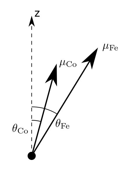
In the linear regime, the small angle between the magnetic moments and the axis (giving the direction of the ground state magnetization) depends on the strength of the external perturbation, cf. figure 1. It is zero in the ground state. Suppose the projection of the tilted moments to the plane be with a small parameter linearly dependent on the strength of the external field. The component of the (normalized) eigenvector of the loss matrix is . Then
| (9) |
The ratio between the angles of different constituents is independent of .
| (10) |
We model the temperature dependence by a generalized version of the RPA introduced by Callen [22] for simple ordered systems. The thermally averaged magnetic moments are evaluated by calculating
| (11) |
once for every species for CPA, and once for every site in the system for MC calculations. Here,
| (12) |
with the density of states for the species or lattice site in question.
2.1 MC calculations
For the direct numerical averaging of the susceptibility, we use a supercell with 202020 primitive unit cells and periodic boundary conditions. The generation of the random occupation is done by means of pseudorandom numbers. The obtained real space susceptibility is averaged over 30 different configurations. With these parameters, the results are converged. They will be presented in chapter 3. The susceptibility of each configuration is given in real space by
| (13) |
where bold symbols denote matrices in the site basis and
| (14) |
2.2 Coherent Potential Approximation
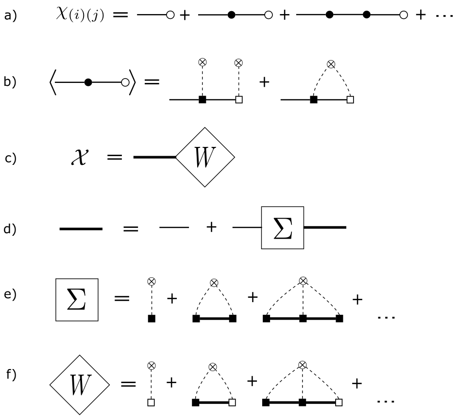
Within the CPA formalism, the equation of motion 3 is used to generate a series expansion of the susceptibility. The series is the Fourier transformed using equation 7, which leads to the series written diagrammatically in figure 2 a) [29]. The following symbols are used:
-
•
The -matrix
(15) where
(16) is represented by a filled square.
-
•
The filled circle represents a - matrix
(17) -
•
An empty square stands for a -matrix:
(18) -
•
The -matrix is depicted as an empty circle and is given by
(19) -
•
The propagator of uncoupled magnetic moments, represented by a solid line, is given as
(20) -
•
A cumulant of order is represented by a crossed circle, where the order is given by the number of dashed lines ending at it.
Furthermore, two rules for the interpretation of the diagrams need to be followed:
-
1.
The elements brought together in a diagram undergo a matrix multiplication in the -space. The corresponding matrix indices are written as subscripts in the definitions above.
-
2.
Every internal free propagator is assigned a momentum which is integrated over:
(21)
Averaging over all possible configurations needs to be done carefully to obtain correct magnetic properties of the material. The average of the Fourier transformed second term in series 3 is depicted in figure 2 b). Starting from the fourth order diagrams, diagrams with crossed dashed lines will appear. These diagrams correspond to correlations between the occupation of different sites. In our approach, these diagrams are neglected. Since the averaged diagrams consist of two different types of vertices (filled and empty squares), the averaged susceptibility can be written as a product of two quantities as shown in figure 2 c). These two quantities are defined in 2 d) - f). It can be shown that all non-crossed diagrams can be constructed with these definitions. The self consistency of the method is evident from the fact that the self energy (figure 2 e)) depends on the effective medium propagator which in turn depends on the self energy. Further details of the theory are given in references [14, 19, 30].
3 Results
Magnetic moments and exchange parameters of iron-cobalt alloys at various concentrations were evaluated using a first-principles Green-function method within a generalized gradient approximation of density functional theory [31]. The method is designed for bulk materials, surfaces, interfaces and real space clusters [32, 33, 34]. The resulting magnetic moments read and . The average magnetic moment per atom is given by the arithmetic mean of the constituents magnetic moments (for 50:50 alloys) and reads , which is in good agreement with experimental results [35]. The impact of disorder on the electronic structure was taken into account within the electronic CPA [36] implemented within multiple scattering theory [37]. Exchange interaction was estimated using the magnetic force theorem [26] formulated for substitutional alloys within the CPA approach [38]. Although both iron and cobalt are known for long ranged interaction between the magnetic moments, the results presented in this section use only 12 shells of neighbors because of computational limits. To ensure the convergence of spin waves with the number of neighbor shells and supercell size, several calculations were performed for 30 neighbor shells showing essentially the same results as with 12 shells. We consider only the disordered alloy \chFe_0.5Co_0.5.
For better comparability the bcc structure was taken in all calculations. Furthermore, the interaction parameters are
held constant (at their value at ). Both MC and CPA calculations are done at
complex energies with a small imaginary part
.
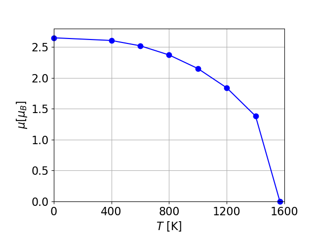
The resulting temperature dependence of the magnetic moments is shown in figure 3. Although the RPA is known to underestimate the Curie temperature [39], we obtain a Curie temperature above the experimental values of K [12, 13]. This behavior can be partly explained by the fact that the real FeCo system will perform a structural phase transition, while in the calculations the structure (bcc) was fixed.
3.1 Eigenmodes at
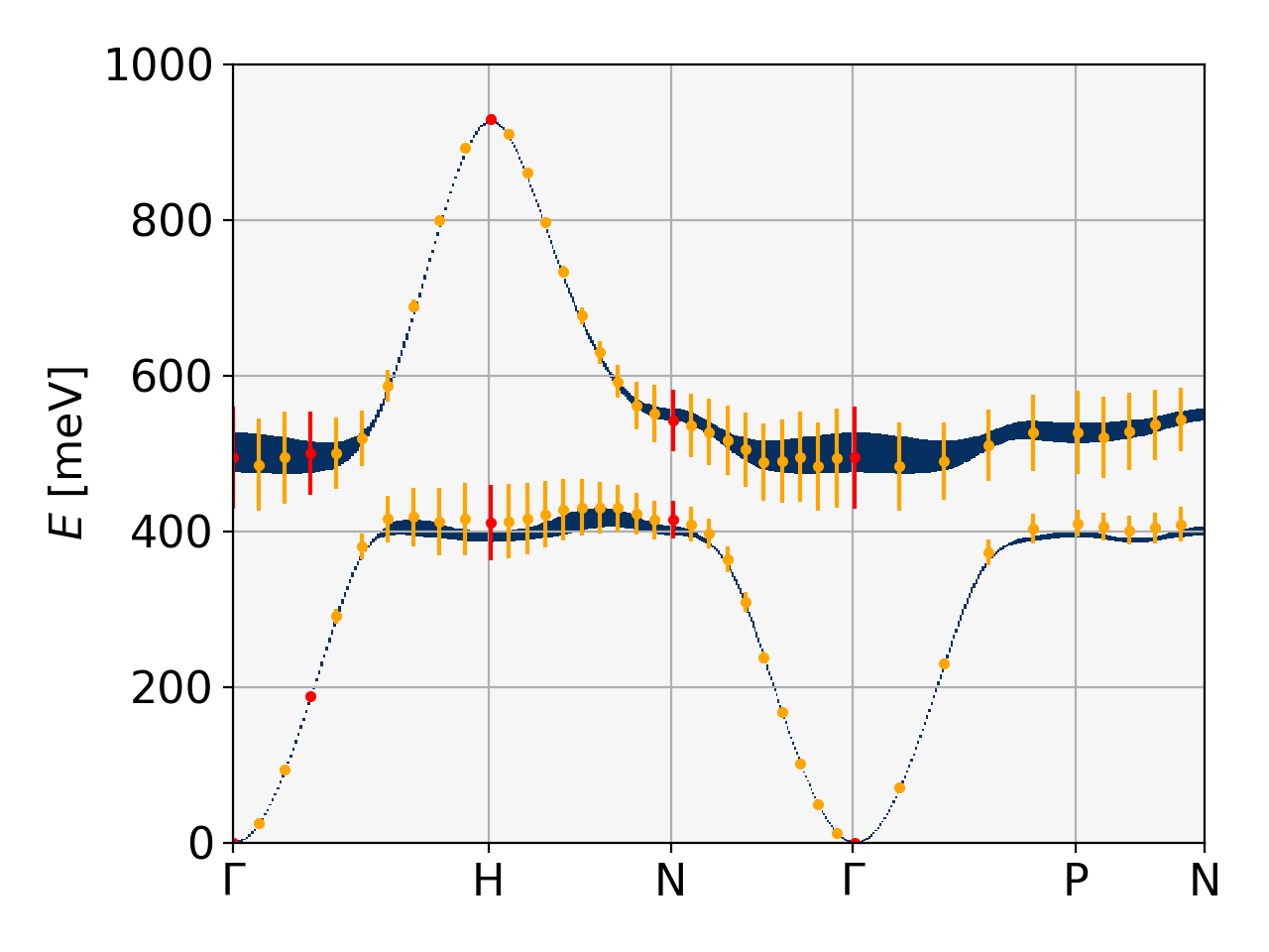
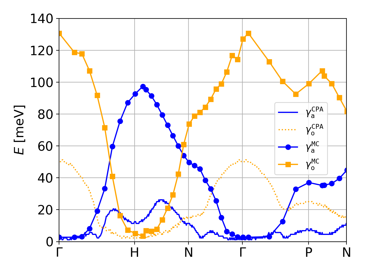
The magnonic spectra (cf. figure 4) obtained using
both methods are basically identical. In the left plot of figure
4, the density plot in the background represents the
imaginary part of the CPA susceptibility while the dots stand for
the position of the susceptibility peaks within the MC. The errorbars
at the points represent the full width at half maximum of the peaks. The same holds for the
width of the line and the CPA results. Due to the finite size of
the supercell, the MC can only give meaningful results for a
discrete set of points within the Brillouin zone (BZ). The spectra are in good agreement with other results for ordered FeCo systems [40, 41] (note that the spectra in these references are calculated for a CsCl structure).
We obtain a spin wave stiffness of meVÅ at K. Experimental values range from meVÅ [42](at K) to meVÅ [43](thin film at room temperature). We note that the long range interaction between magnetic moments which was neglected in this work due to computational limits may influence the magnonic spectrum, especially close to the point and therefore also affect the spin stiffness.
It can clearly be seen that the CPA systematically underestimates
the width of the peaks. In the right plot of figure
4, we show the full width at half maximum
for the acoustic and optic modes within the CPA and the MC
calculations. Although the absolute values of the damping is
different, the general trend of through the considered paths
in the BZ is very similar. The fact that the MC calculations give
much larger widths indicates that non-local effects play an essential
role in the damping of magnons. Recent studies [44, 45, 46] reveal, that non-local effects also play an important role in the Ising model. Although the Ising model only captures nearest neighbor spin interaction, in 3D a term with an effective long range interaction appears in the partition function [45]. Although the results of these studies cannot be directly applied to our model, they represent a further hint at the presence and influence of non-local effects.
The CPA predicts [14] that at the 50% concentration of cobalt the bandgap is still present. However, the more realistic estimation of the magnon damping using the MC method tends to suggest that the significant widening of the magnon modes might lead to effective closing of the gap.
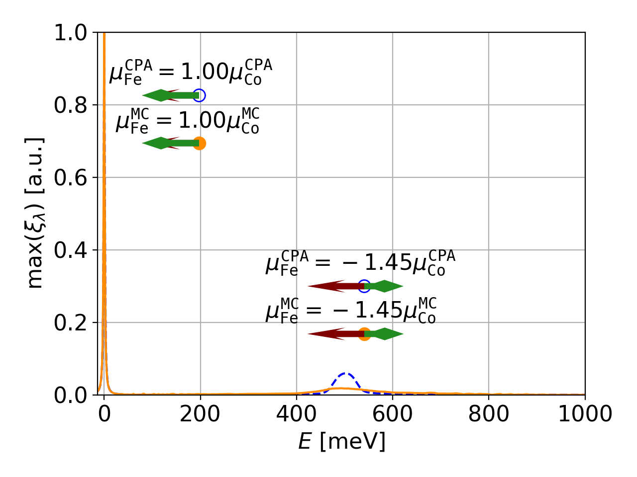
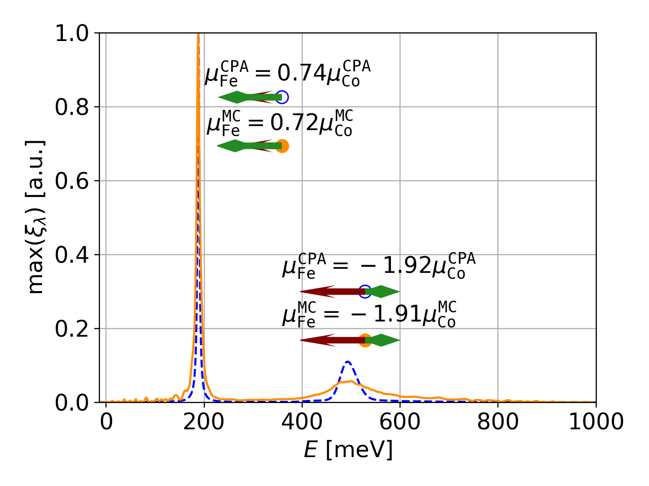
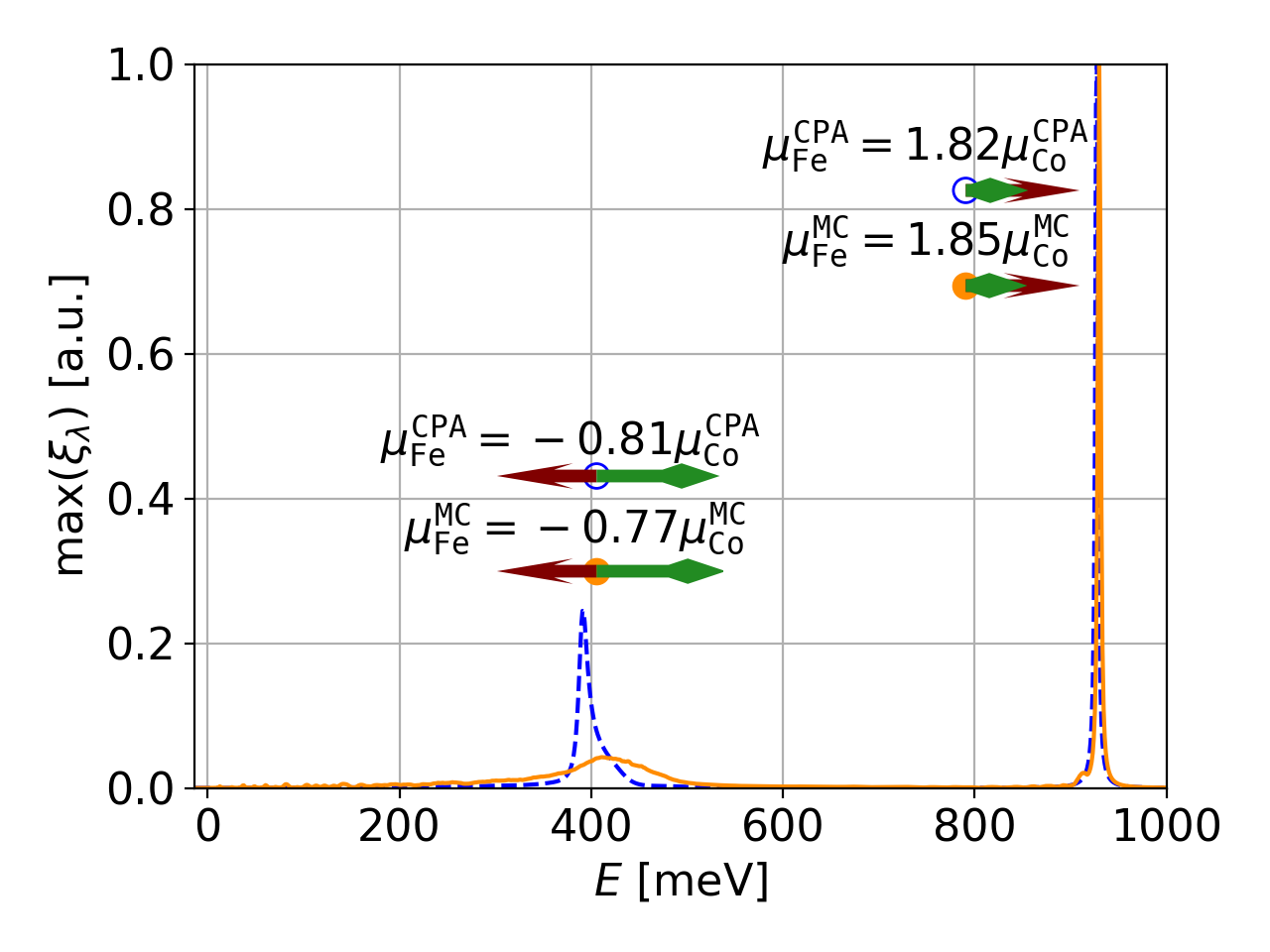
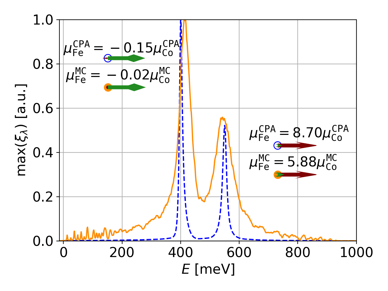
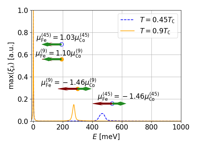
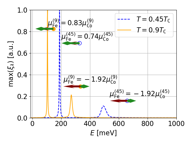
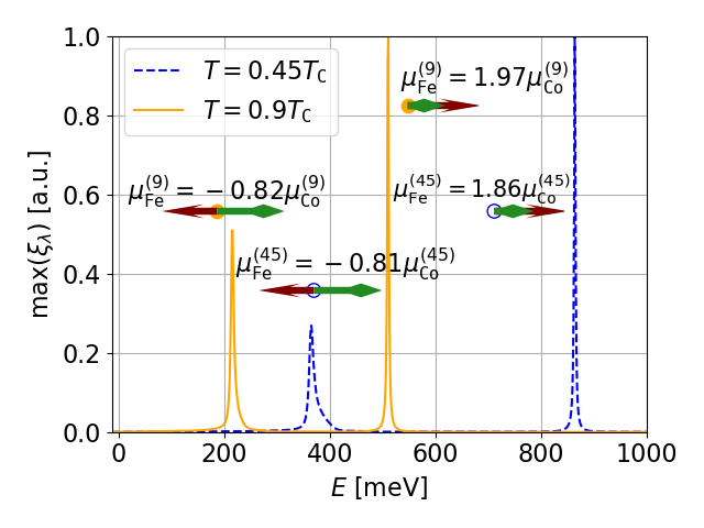
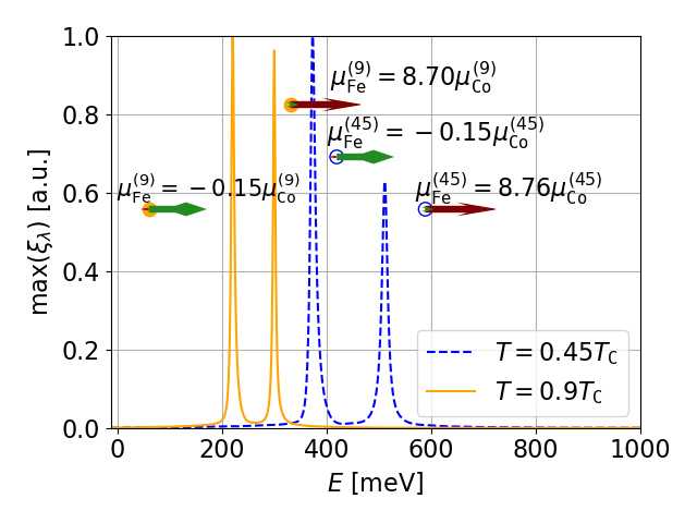
The red dots in figure 4 mark the -points for which the spatial shapes of the magnon modes will be analyzed in more detail now. In figure 5 the eigenvalues and eigenvectors of the loss matrix are shown at different symmetry points in the BZ and . The maximal eigenvalue at the point for (figure 5, top left) exhibits the Goldstone mode at zero energy, i.e. the mode where the moments of both constituents are tilted by the same amount.
As already mentioned, we explain the larger width of the MC peaks with the influence of correlation effects between different sites, which the CPA cannot account for. The appearance of smaller peaks at regions where the CPA susceptibility is effectively zero is a further effect caused by non local effects. An interesting fact is that at the N point (c.f. bottom right plot in figure 5) essentially only one of the constituents precesses for both the acoustic and the optic mode. Unfortunately, the direct measurement of the shape very challenging but recent studies suggest that it could be realized on the surface of a 2D magnet using atomic resolution inelastic scanning tunneling microscopy [47].
Generally, we come to the conclusion that the CPA is able to precisely give the magnetic properties of this iron cobalt alloy apart from a systematic underestimation of the magnon damping.
3.2 Spatial form of the eigenmodes
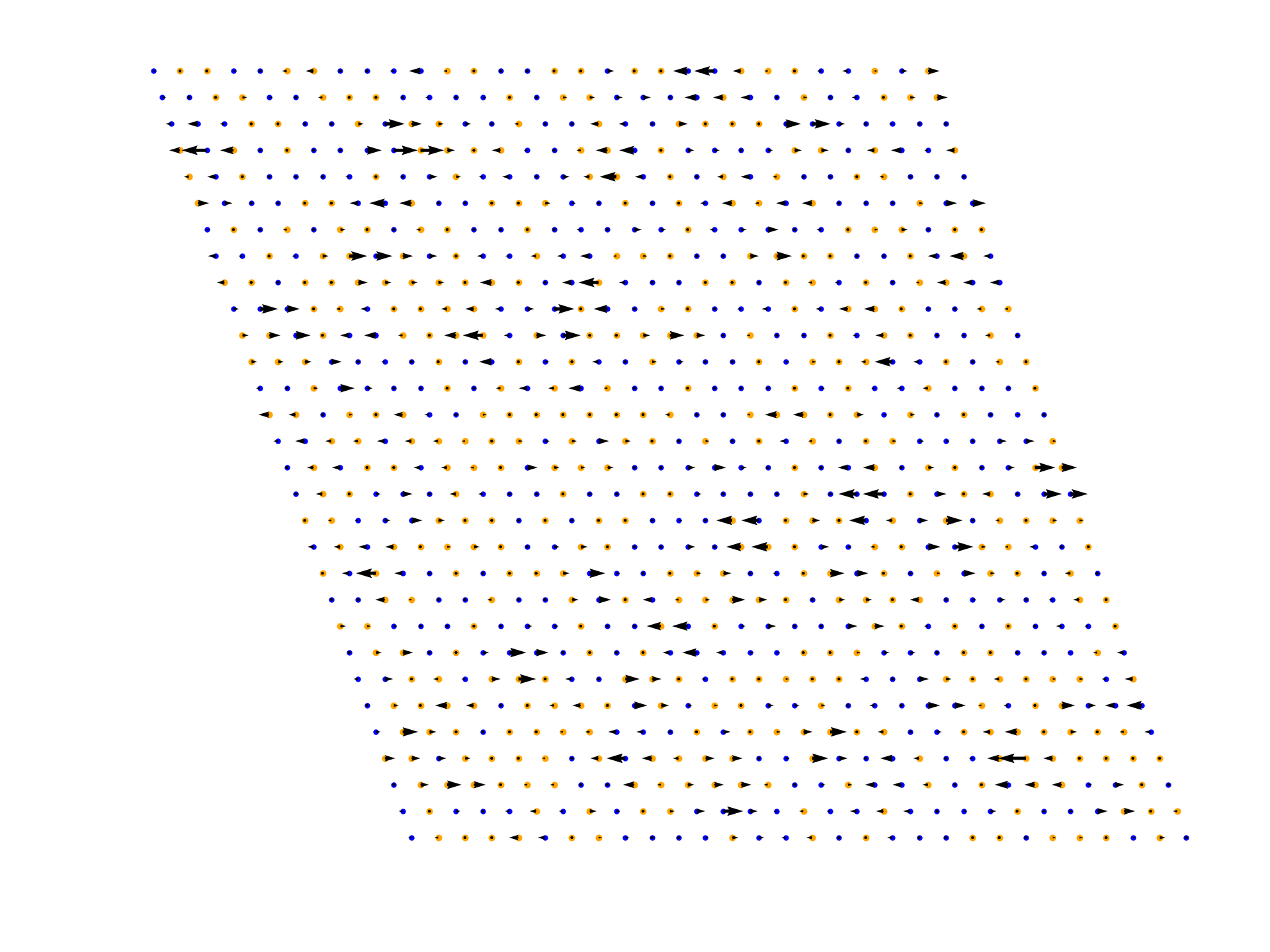
Through the diagonalization of the susceptibility in real space (equation 3), the spatial eigenvectors at a certain energy can be directly found through the loss matrix (equation 8). We did so calculating the real space susceptibility of one specific random configuration in a 303010 atom supercell. The eigenmode corresponding to the highest eigenvalue of the loss matrix at is depicted for this specific random configuration in figure 6. This figure shows one plane of the supercell corresponding to with the primitive lattice vectors , and . The orange dots correspond to \chCo atoms while the blue dots represent \chFe atoms. It is assumed that in the magnetic ground state all magnetic moments are oriented orthogonal to the plane depicted. The in-plane components of the magnetic moments of this particular mode are represented by the arrows. Interestingly, we observe that the mode shown in figure 6 features multiple small clusters of precessing moments.
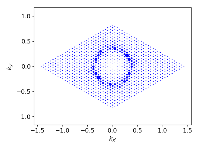
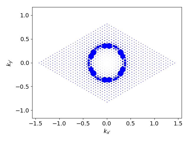
We further analyze the eigenmode by performing a Fourier analysis of the
| (22) |
with the positions of the atoms and the number of atoms in our case. The result is depicted in figure 7 for a plane in the BZ. The dominant contributions arise from wavevectors lying on an circle. In an ordered system, the circle would be the cross section of the constant energy surface in reciprocal space. Due to the disorder, Bloch waves cease to be eigenstates of the system (the corresponding peaks acquire finite widths) and the eigenstates pick up Fourier components outside of a single energy surface. Finally, we further analyze the loss matrix by writing its spectral representation
| (23) |
with the eigenvalues and eigenvectors . The projection of the loss matrix to plain wave states is then given by
| (24) |
which represents a weighted sum of Fourier components. The plain wave projection for all eigenvalues larger than , with the highest eigenvalue , is given in figure 7. Considering all the modes with significant eigenvalues at this energy recovers the picture of the constant energy surface similar to the one of an ordered system. While a single eigenmode is clearly different from a Bloch wave, the dynamics of the entire system resembles the one of the ordered system. In a sense, the Fourier transformation recovers the self-averaging property of the spin dynamics in disordered magnets.
3.3 Eigenmodes at finite temperatures
Next, we investigate the change of the eigenmodes with temperature. It turned out that our realization of the RPA in combination with the MC calculations is computationally too expensive for the system size we are considering here. Therefore, we restrict this discussion to the CPA+RPA results and stress again the agreement of CPA and MC shown in the previous section especially when it comes to the spatial form of the modes. We recall that the widely used RPA [48, 49, 50] cannot account for the temperature broadening of the magnon modes [14] such that we must restrict ourselves to the analysis of the impact of the temperature on the shapes of magnetic modes, cf. figure 8. Our calculations suggest that the spatial shape of the modes is independent of temperature.
4 Summary
We provided a thorough analysis of the magnonic modes in a disordered iron cobalt alloy using two complementary numerical schemes. The MC and the CPA give basically the same magnonic properties apart from the disorder induced width of the peaks in the magnonic spectrum. We explain this discrepancy with non-local effects which the single site CPA cannot account for. Interestingly, we found that the acoustic and optic mode at the N point features the precession of only one of the constituents’ magnetic moments. The eigenspectrum analysis of the loss matrix in real space reveals that the eigenmodes involve many small clusters of precessing magnetic moments. We are convinced that such real space effects can be used to effectively excite only defining parts of the magnonic crystal and thus gain additional precise control over the spin dynamics of the system. Finally, it turns out that the spatial shape of the modes is basically invariant with respect to temperature.
References
- [1] Chumak A V, Vasyuchka V I, Serga A A and Hillebrands B 2015 Nature Physics 11 453–461
- [2] Bloch F 1930 Zeitschrift für Physik 61 206–219
- [3] Chumak A V, Serga A A and Hillebrands B 2017 Journal of Physics D: Applied Physics 50 244001
- [4] Nikitov S, Tailhades P and Tsai C 2001 Journal of Magnetism and Magnetic Materials 236 320–330
- [5] Krawczyk M and Grundler D 2014 Journal of Physics: Condensed Matter 26 123202
- [6] Lenk B, Ulrichs H, Garbs F and Münzenberg M 2011 Physics Reports 507 107–136
- [7] Sadovnikov A V, Beginin E N, Odincov S A, Sheshukova S E, Sharaevskii Y P, Stognij A I and Nikitov S A 2016 Applied Physics Letters 108 172411
- [8] Sadovnikov A V, Gubanov V A, Sheshukova S E, Sharaevskii Y P and Nikitov S A 2018 Physical Review Applied 9
- [9] Sheshukova S E, Morozova M A, Beginin E N, Sharaevskii Y P and Nikitov S A 2013 Physics of Wave Phenomena 21 304–309
- [10] Zakeri K 2018 Physica C: Superconductivity and its Applications 549 164–170
- [11] Buczek P, Ernst A, Bruno P and Sandratskii L M 2009 Physical Review Letters 102
- [12] Normanton A S, Bloomfield P E, Sale F R and Argent B B 1975 Metal Science 9 510–517
- [13] Nishizawa T and Ishida K 1984 Bulletin of Alloy Phase Diagrams 5 250–259
- [14] Paischer S, Buczek P A, Buczek N, Eilmsteiner D and Ernst A Spin waves in disordered FeCo magnonic crystal at finite temperatures , to be published URL arXiv:2009.04712
- [15] Buczek P, Ernst A and Sandratskii L M 2011 Physical Review Letters 106
- [16] Buczek P, Ernst A and Sandratskii L M 2011 Physical Review B 84
- [17] Zakeri K, Zhang Y, Chuang T H and Kirschner J 2012 Physical Review Letters 108
- [18] Qin H J, Zakeri K, Ernst A, Sandratskii L M, Buczek P, Marmodoro A, Chuang T H, Zhang Y and Kirschner J 2015 Nature Communications 6
- [19] Buczek P, Sandratskii L M, Buczek N, Thomas S, Vignale G and Ernst A 2016 Physical Review B 94
- [20] Edström A, Werwiński M, Iuşan D, Rusz J, Eriksson O, Skokov K P, Radulov I A, Ener S, Kuz'min M D, Hong J, Fries M, Karpenkov D Y, Gutfleisch O, Toson P and Fidler J 2015 Physical Review B 92 174413
- [21] Rusz J, Bergqvist L, Kudrnovský J and Turek I 2006 Physical Review B 73 214412
- [22] Callen H B 1963 Physical Review 130 890–898
- [23] Şaşıoğlu E, Friedrich C and Blügel S 2013 Physical Review B 87
- [24] Staunton J B, Poulter J, Ginatempo B, Bruno E and Johnson D D 1999 Phys. Rev. Lett. 82(16) 3340–3343 URL https://link.aps.org/doi/10.1103/PhysRevLett.82.3340
- [25] Staunton J B, Poulter J, Ginatempo B, Bruno E and Johnson D D 2000 Phys. Rev. B 62(2) 1075–1082 URL https://link.aps.org/doi/10.1103/PhysRevB.62.1075
- [26] Liechtenstein A, Katsnelson M, Antropov V and Gubanov V 1987 Journal of Magnetism and Magnetic Materials 67 65–74
- [27] Nolting W and Ramakanth A 2009 Quantum Theory of Magnetism (Springer)
- [28] Kubo R 1966 Reports on Progress in Physics 29 255–284
- [29] Yonezawa F 1968 Progress of Theoretical Physics 40 734–757
- [30] Buczek P, Thomas S, Marmodoro A, Buczek N, Zubizarreta X, Hoffmann M, Balashov T, Wulfhekel W, Zakeri K and Ernst A 2018 Journal of Physics: Condensed Matter 30 423001
- [31] Perdew J P, Burke K and Ernzerhof M 1996 Physical Review Letters 77 3865–3868 URL http://link.aps.org/abstract/PRL/v77/p3865
- [32] Lüders M, Ernst A, Temmerman W M, Szotek Z and Durham P J 2001 Journal of Physics: Condensed Matter 13 8587–8606 URL http://stacks.iop.org/0953-8984/13/8587
- [33] Geilhufe M, Achilles S, Köbis M A, Arnold M, Mertig I, Hergert W and Ernst A 2015 Journal of Physics: Condensed Matter 27 435202
- [34] Hoffmann M, Ernst A, Hergert W, Antonov V N, Adeagbo W A, Geilhufe R M and Hamed H B 2020 physica status solidi (b) 257 1900671 (Preprint https://onlinelibrary.wiley.com/doi/pdf/10.1002/pssb.201900671) URL https://onlinelibrary.wiley.com/doi/abs/10.1002/pssb.201900671
- [35] Goldman J E and Smoluchowski R 1949 Physical Review 75 310–311
- [36] Soven P 1967 Physical Review 156 809–813 URL http://link.aps.org/doi/10.1103/PhysRev.156.809
- [37] Gyorffy B L 1972 Physical Review B 5 2382–2384 URL http://link.aps.org/doi/10.1103/PhysRevB.5.2382
- [38] Turek I, Kudrnovský J, Drchal V and Bruno P 2006 Philosophical Magazine 86 1713–1752 URL http://www.informaworld.com/10.1080/14786430500504048
- [39] Rusz J, Turek I and Diviš M 2005 Physical Review B 71
- [40] Okumura H, Sato K and Kotani T 2019 Physical Review B 100 054419
- [41] Grotheer O, Ederer C and Fähnle M 2001 Physical Review B 63 100401
- [42] Lowde R D, Shimizu M, Stringfellow M W and Torrie B H 1965 Physical Review Letters 14 698–700
- [43] Liu X, Sooryakumar R, Gutierrez C J and Prinz G A 1994 Journal of Applied Physics 75 7021–7023
- [44] Zhang Z D 2007 Philosophical Magazine 87 5309–5419
- [45] Zhang Z 2017 Journal of Physics: Conference Series 827 012001
- [46] Zhang Z 2020 Journal of Materials Science & Technology 44 116–120
- [47] Hirjibehedin C F 2006 Science 312 1021–1024
- [48] Tang G X and Nolting W 2006 Physical Review B 73
- [49] Bouzerar G and Bruno P 2002 Physical Review B 66
- [50] Matsubara T 1973 Progress of Theoretical Physics Supplement 53 202–221