Spatiotemporal Registration for Event-based Visual Odometry

Abstract

A useful application of event sensing is visual odometry, especially in settings that require high-temporal resolution. The state-of-the-art method of contrast maximisation recovers the motion from a batch of events by maximising the contrast of the image of warped events. However, the cost scales with image resolution and the temporal resolution can be limited by the need for large batch sizes to yield sufficient structure in the contrast image. In this work, we propose spatiotemporal registration as a compelling technique for event-based rotational motion estimation. We theoretically justify the approach and establish its fundamental and practical advantages over contrast maximisation. In particular, spatiotemporal registration also produces feature tracks as a by-product, which directly supports an efficient visual odometry pipeline with graph-based optimisation for motion averaging. The simplicity of our visual odometry pipeline allows it to process more than 1 M events/second. We also contribute a new event dataset for visual odometry, where motion sequences with large velocity variations were acquired using a high-precision robot arm.

1 Introduction

Due to their ability to asynchronously detect intensity changes, event sensors are well suited for conducting visual odometry (VO) in applications that require high temporal resolution [16, 28, 43, 26, 41], , high-agility robotic manipulation, fast manoeuvring aerial vehicles. However, to fully reap the benefits of event sensing for VO, efficient algorithms are required to process event streams with low-latency to accurately recover the experienced motion.

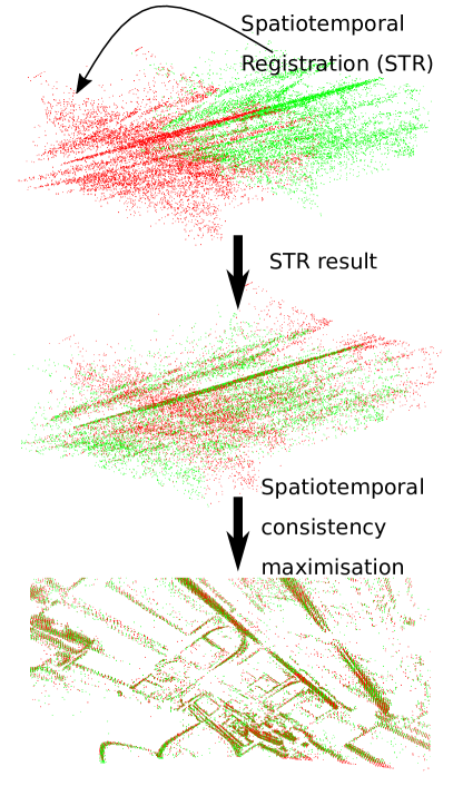
Figure 1: Conceptual difference between contrast maximisation and spatiotemporal registration for event-based motion estimation.

An event sensor produces an event stream $\mathcal{S}=\{\mathbf{e}\}$, where each $\mathbf{e}=(\mathbf{u},t,p)$ is a tuple containing the 2D image coordinates $\mathbf{u}$, time stamp $t$ and polarity $p$ associated with a brightness change that exceeded the preset threshold. In scenarios where the event camera (i.e., event sensor plus optics and other components) moves in a static environment, the events are triggered mainly by the camera motion. The goal of VO is to recover the camera motion from $\mathcal{S}$.

Many event-based VO methods [47, 35, 20, 34] conduct “batching”, where small subsets of $\mathcal{S}$ are processed incrementally. Each batch $\mathcal{E}=\{\mathbf{e}_{i}\}^{N}_{i=1}\subset\mathcal{S}$ is acquired over a time window $\mathcal{T}=[\alpha,\beta]$, where each $\mathbf{e}_{i}=(\mathbf{u}_{i},t_{i},p_{i})$ is associated with a 3D point in the camera FOV that triggered $\mathbf{e}_{i}$ at time $t_{i}\in\mathcal{T}$. The core task is to estimate the relative motion $\mathcal{M}$ between $\alpha$ and $\beta$ from $\mathcal{E}$. The estimated $\mathcal{M}$ is then subject to the broader VO pipeline (more in Sec. 2).

1.1 Contrast maximisation

A state-of-the-art approach to estimate $\mathcal{M}$ from $\mathcal{E}$ is contrast maximisation (CM) [19]. Parametrising $\mathcal{M}$ by a vector $\bm{\omega}\in\Omega$ and letting $\mathcal{D}=\{\mathbf{x}_{j}\}_{j=1}^{P}$ be the image domain (the set of pixel coordinates) of the event sensor, each candidate $\bm{\omega}$ yields the image of warped events (IWE)

$$H(\mathbf{x}_{j};\bm{\omega})=\sum_{i=1}^{N}\kappa_{\delta}(\mathbf{x}_{j}-f(\mathbf{u}_{i},t_{i};\,\bm{\omega})),$$ (1)

where $f$ warps $\mathbf{u}_{i}$ to a position in $H$ by reversing the motion $\bm{\omega}$ from $t_{i}$ to the start of $\mathcal{T}$. The form of $f$ depends on the type of motion $\mathcal{M}$(see [19] for details). The warped events are aggregated by a kernel $\kappa_{\delta}$ with bandwidth $\delta$, ,

$$\kappa_{\delta}(\mathbf{x})=\exp(\|\mathbf{x}\|_{2}/2\delta^{2}).$$ (2)

The contrast of $H$ is given by

$$C(\bm{\omega})=\dfrac{1}{P}\sum_{j=1}^{P}(H(\mathbf{x}_{j};\bm{\omega})-\mu(\bm{\omega}))^{2},$$ (3)

where $\mu(\bm{\omega})$ is the mean intensity of $H$ the image. Both $C$ and $\mu$ are functions of $\bm{\omega}$ since $H$ is dependent on $\bm{\omega}$. CM estimates $\bm{\omega}$ by maximising $C(\bm{\omega})$, the intuition being that the correct $\bm{\omega}$ will yield a sharp image $H$; see Fig. 1.

Previous studies found CM effective in a number of event-based VO tasks [19], especially where $\mathcal{M}$ is a rotation, i.e., $\Omega=SO(3)$. However, there are a couple of fundamental weaknesses in CM, as described in the following.

Computational cost

Maximising $C(\bm{\omega})$ can be done using conjugate gradient [19] and branch-and-bound [25]. Note that the cost to compute (3) depends on both

• the number of pixels $P$; and

• the number of events $N$ in the batch $\mathcal{E}$.

While $P$ is a constant of the event sensor, $N$ depends on the motion speed and scene complexity. A higher $P$ increases the FOV and hence tends to increase $N$, however, the cost of $C(\bm{\omega})$ will increase with $P$ even if $N$ is constant.

The basic analysis above indicates that the cost of CM (regardless of the algorithm) will also scale with both $P$ and $N$. Fig. 2 plots the runtime of CM (using conjugate gradient) on input instances with increasing $P$ and constant $N$, which shows a clear uptrend. While early event sensors have low resolutions (, $240\times 180$ on iniVation Davis 240C), current sensors can have up to 1 Megapixels (, $1280\times 720$ on Prophesee 720P CD, $1280\times 800$ on CeleX-V). Following industry trends, event sensors will likely continue to increase in resolution. To maintain the efficiency of CM on high-resolution sensors, a separate heuristic to reduce the “image resolution” is needed (note that this is different sparsifying $\mathcal{E}$ by reducing the number of events $N$).

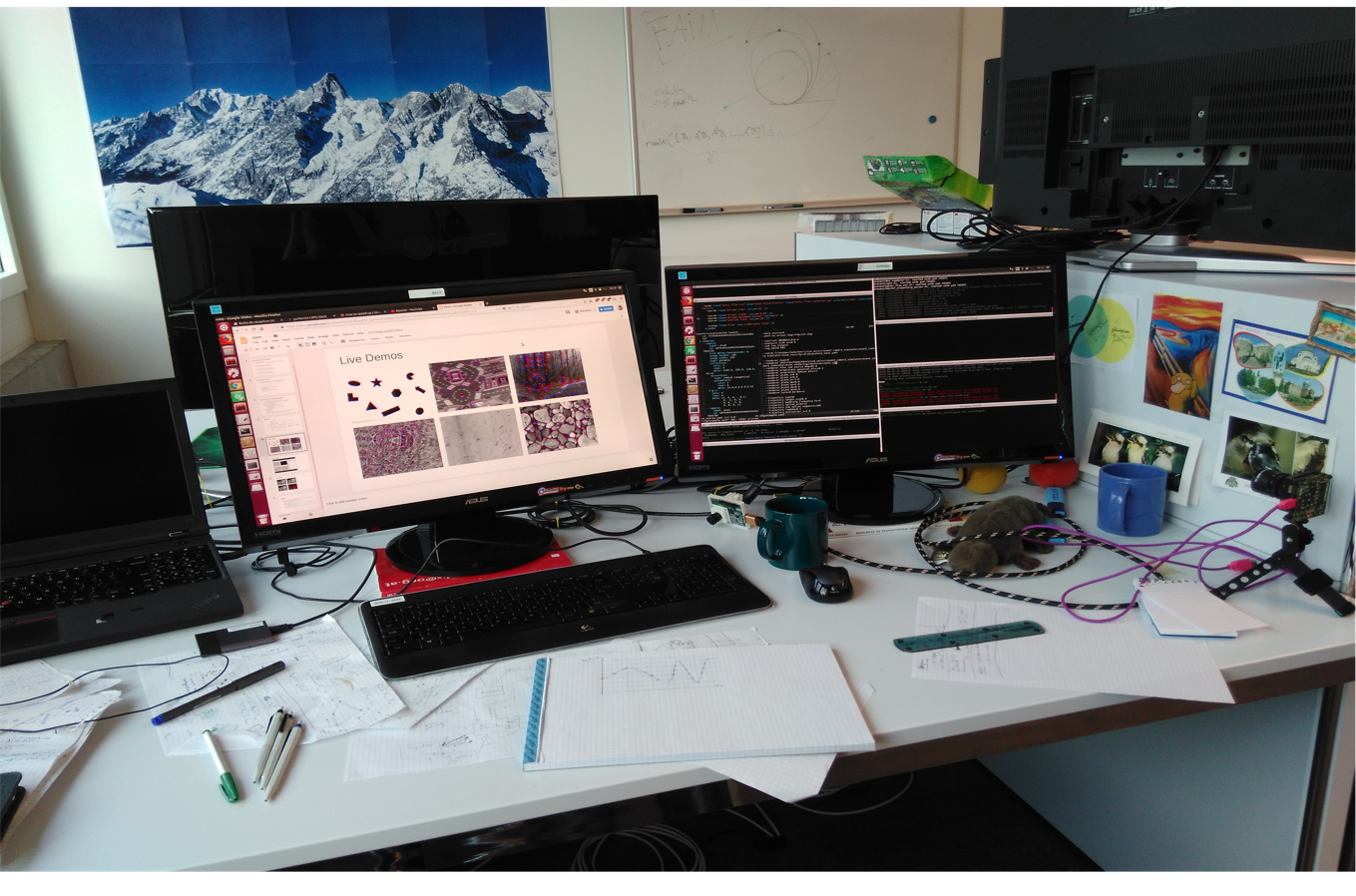
(a) Original scene.

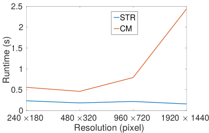
(b) Runtime vs num. of pixels $P$.

Figure 2: Using the image in panel (a) as input to ESIM [33], we generated synthetic event batches as outputs of event sensors of varying resolution, from $P=240\times 180$ to $P=1920\times 1440$ pixels. By tuning the duration $|\mathcal{T}|$, the batch size $N$ was fixed at $15,000$. Panel (b) illustrates the average runtime of CM and STR on the generated data as a function of resolution.

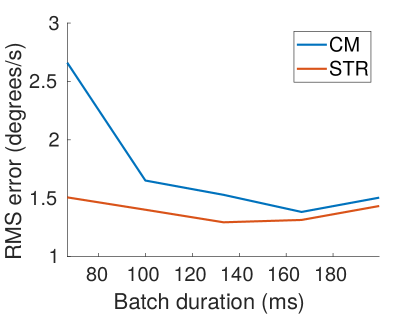
(a) Error vs batch duration $|\mathcal{T}|$.

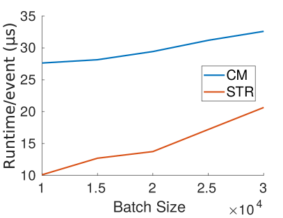
(b) Runtime vs batch size $N$.

Figure 3: Motion estimation error and runtime of CM and STR.

Temporal resolution

Intuitively the accuracy of estimating $\mathcal{M}$ depends on capturing sufficient “structure” in $\mathcal{E}$. For a fixed scene and motion rate, the amount of structure in $\mathcal{E}$ increases with the duration $|\mathcal{T}|=\beta-\alpha$ [27]. Conversely to achieve VO with high temporal resolution, $|\mathcal{T}|$ should be as small as possible to minimise batching effects. The conflicting demands indicate a maximum temporal resolution achievable by an event-based motion estimation technique.

Fig. 3 shows the motion estimation accuracy of CM on batches $\mathcal{E}$ of different durations $|\mathcal{T}|$ from sequence PureRot_Mid_Off of our event dataset (Sec. 3.3). Unlike the experiment in Fig. 2, the number of events $N$ were varied according to $|\mathcal{T}|$. Note the degradation in accuracy as $|\mathcal{T}|$ decreases (i.e., $N$ decreases), which indicates a lower temporal resolution of CM (more results in Sec. 3.4).

1.2 Our contributions

We propose spatiotemporal registration (STR) as a cogent alternative to CM; see Fig. 1 on the concept of STR. Despite the relative simplicity of STR, it has not been thoroughly investigated for event-based motion estimation. Specifically, we will justify STR by examining the conditions in which it is valid (Sec. 3) and demonstrate that it is generally as accurate for rotational motion estimation but does not suffer from the fundamental weaknesses of CM demonstrated in Sec. 1.1 (more results in Sec. 3.4).

Further, unlike CM, STR produces feature correspondences as a by-product (see Fig. 1). This directly enables a novel event-based VO pipeline (Sec. 4) that conducts feature tracking and motion averaging. To support our experiments, we build a new event dataset for VO using a high-precision robot arm (Sec. 3.3 and our dateset website).

2 Related works

The CM framework has been improved in several directions. Stoffregen et al. [38] adjusted the contrast objective by introducing “sparsity” to improve the accuracy of motion estimation. They later integrated CM into the segmentation task [37]. Globally optimal CM was proposed in [25, 32], where [25] further accelerated the algorithm by integer quadratic programming relaxation. Seok and Lim [36] dropped the constant velocity assumption and replaced linear interpolation by Bezier curve. In general, the improvements above tend to increase cost, which discourage real-time applications.

Closer to our work is Nunes and Demiris [31] who proposed an entropy minimisation framework (EM) for event-based motion estimation. Their approach maximises the similarity (minimising the entropy) between the feature vector of events. Like our proposed STR method, EM also obviates the need to compute the image of warped events. However, although a truncated kernel was used to accelerate their algorithm, EM is still too expensive for online application, as results in Sec. 3.4 will show.

The techniques surveyed above can be considered “direct methods” since all events are utilised in the computation. Unlike direct methods, “feature-based” methods achieve VO by detecting and tracking simple structures in the event data, such as circles [30] and lines [14]. To handle the more complex scene, traditional frame-based feature detectors are utilised on motion-compensated event images [34, 41], frames [39, 24] and time surfaces (TS) [40, 26, 4] recently. A TS [17] is a reconstructed image that each pixel records the temporal information of the last event as “intensity” of the image. Based on the detected features, Alzugarary et al. [3] propose a descriptor and a tracker that employed the descriptors for event data. Zhu et al. [48] present a feature tracking based on Expectation Maximisation (EM). They later propose visual-inertial odometry (VIO) [51] system by fusing IMU and their feature trackers. On the other hand,  [34] utilises Kanade–Lucas–Tomasi feature tracker [6] on the motion-compensated event images with the motion from IMU. Note that all the feature-based methods highly rely on a different heuristic for keypoint detection and tracking, which can quickly lose track without IMU.

Learning-based method has gained more attention recently, and there have been several works that solve the event-based VO with unsupervised learning [50, 44], and spiking network [21]. Both [50] and  [44] follow the framework and architecture from SfMLearner [46] and propose some changes for event-based setting. However, Since lack of training data, all learning-based methods cannot be generalised to different environments, which overfitting to the training data. Moreover,  [45, 8] show the limitations in pure rotation motion of learning-based method.

3 Spatiotemporal registration

In this section, we describe the proposed event-based relative motion estimation technique, including its fundamental underpinnings and optimisation algorithm.

3.1 Motion model

For a batch of events $\mathcal{E}$ acquired over time duration $\mathcal{T}=[\alpha,\beta]$, we represent using

$$\mathbf{M}_{t}=\left[\begin{matrix}\mathbf{R}_{t}&\mathbf{c}_{t}\\ \mathbf{0}&1\end{matrix}\right]$$ (4)

the absolute pose of the event camera at time $t\in\mathcal{T}$, where $\mathbf{R}_{t}\in SO(3)$ and $\mathbf{c}_{t}\in\mathbb{R}^{3}$ are respectively the absolute orientation and position of the camera at the same time $t$. Let $a$ and $b$ be two time instances in $\mathcal{T}$, where

$$\alpha\leq a\leq b\leq\beta.$$ (5)

The relative motion between $a$ and $b$ is given by

$$\mathbf{M}_{a,b} =\mathbf{M}_{b}\mathbf{M}_{a}^{-1}$$

$$=\left[\begin{matrix}\mathbf{R}_{b}\mathbf{R}_{a}^{T}&-\mathbf{R}_{b}\mathbf{R}_{a}^{T}\mathbf{c}_{a}+\mathbf{c}_{b}\\ \mathbf{0}&1\end{matrix}\right].$$ (6)

We follow many previous works [25, 20, 32, 21] to focus on rotational odometry, which is useful for a number of applications, e.g., video stabilisation [19], panorama construction [23], star tracking [13, 5]. This allows to assume pure rotational motion for $\mathbf{M}_{t}$, where $\mathbf{c}_{t}=\mathbf{0}$ for all $t$ and the relative motion (3.1) reduces to the relative rotation

$$\mathbf{M}_{a,b} =\left[\begin{matrix}\mathbf{R}_{b}\mathbf{R}_{a}^{T}&\mathbf{0}\\ \mathbf{0}&1\end{matrix}\right].$$ (7)

More succinctly, the relative rotation between $a$ and $b$ is

$$\mathbf{R}_{a,b} :=\mathbf{R}_{b}\mathbf{R}_{a}^{T},$$ (8)

and setting $a=\alpha$ and $b=\beta$ yields $\mathbf{R}_{\alpha,\beta}$, which is the target relative motion $\mathcal{M}$ to be estimated from $\mathcal{E}$.

The short duration of $\mathcal{E}$ (e.g., in the $ms$ range) further motivates to assume constant angular velocity in the period $\mathcal{T}$. Specifically, the absolute orientation can be written as

$$\mathbf{R}_{t}=\exp(\left[t\bm{\omega}\right]_{\times})\exp(\left[\bm{\theta}_{0}\right]_{\times}).$$ (9)

for all $t\in\mathcal{T}$, where $\exp$ is the exponential map. In more detail, vector $\bm{\omega}\in\mathbb{R}^{3}$ defines the angular velocity in period $\mathcal{T}$, where the direction $\hat{\bm{\omega}}$ of $\bm{\omega}$ provides the axis of rotation and the length $\|\bm{\omega}\|_{2}$ of $\mathbf{r}$ specifies the rate of change of the angle of the rotation about $\hat{\bm{\omega}}$. The initial orientation at time $\alpha$ is given by $\bm{\theta}_{0}$, and $t\bm{\omega}$ is the rotational increment on $\bm{\theta}_{0}$ from time $a$ to time $t$.

Applying the BCH formula [1] on (8) yields

$$\mathbf{R}_{a,b} =\exp(\left[b\bm{\omega}\right]_{\times})\exp(\left[-a\bm{\omega}\right]_{\times})$$

$$=\exp(\left[(b-a)\bm{\omega}\right]_{\times}),$$ (10)

where terms involving $\bm{\theta}_{0}$ cancel out, and $\left[a\bm{\omega}\right]_{\times}$ and $\left[b\bm{\omega}\right]_{\times}$ commute and hence the Lie bracket $[\left[a\bm{\omega}\right]_{\times},\left[b\bm{\omega}\right]_{\times}]=0$. The significance of this derivation is encapsulated in the following lemma.

Lemma 1

Assuming that the camera undergoes pure rotational motion with constant angular velocity (9) in the period $\mathcal{T}$, the relative rotation $\mathbf{R}_{a,b}$ between any $a,b\in\mathcal{T}$ with $a\leq b$ depends only on the difference $b-a$ and $\bm{\omega}$.

A straightforward corollary of Lemma 1 is as follows, which is also illustrated in Fig. 4.

Corollary 1

Under the motion model assumed in Lemma 1, $\mathbf{R}_{a,b}=\mathbf{R}_{c,d}$ for all time instances $a,b,c,d$ in the period $\mathcal{T}$ such that $a\leq b$, $c\leq d$ and $b-a=d-c$.

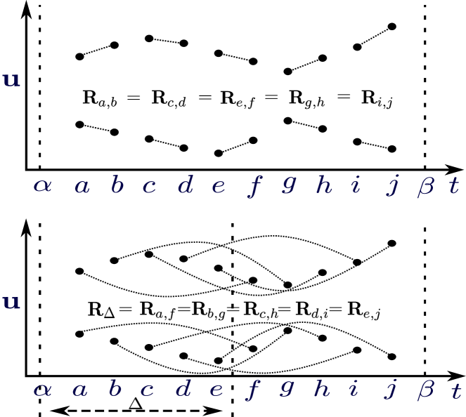
Figure 4: Equivalent relative rotations (see Corollary 1) and their spatiotemporally consistent event correspondences (see Definition 2). In the bottom example, the relative rotations are also equivalent to $\mathbf{R}_{\Delta}$, where $\Delta=0.5(\beta-\alpha)$.

3.2 Event-based relative motion estimation

We exploit the insights above to estimate $\mathcal{M}=\mathbf{R}_{\alpha,\beta}$ from event batch $\mathcal{E}$. First, we define the notion of spatiotemporal consistency and event correspondences.

Definition 1 (Spatiotemporal consistency)

Under the motion model assumed in Lemma 1, a relative rotation $\mathbf{R}_{a,b}$, with $a,b\in\mathcal{T}$ and $a\leq b$, and a pair of events $\mathbf{e}=(\mathbf{u},t,p)$ and $\mathbf{e}^{\prime}=(\mathbf{u}^{\prime},t^{\prime},p^{\prime})$, where $t,t^{\prime}\in\mathcal{T}$ and $t\leq t^{\prime}$, are spatiotemporally consistent if

• $t^{\prime}-t=b-a$ (temporal consistency); and

• $\hat{\mathbf{u}}^{\prime}=\mathbf{R}_{a,b}\hat{\mathbf{u}}$ (geometric consistency),

where $\hat{\mathbf{u}}$ is the backprojected ray (a unit vector)

$$\hat{\mathbf{u}}=\frac{\mathbf{K}^{(1:2)}\tilde{\mathbf{u}}}{\mathbf{K}^{(3)}\tilde{\mathbf{u}}}$$ (11)

of the image point $\mathbf{u}$, where $\tilde{\mathbf{u}}=[\mathbf{u}^{T},1]^{T}$ and $\mathbf{K}^{(1:2)}$ and $\mathbf{K}^{(3)}$ are respectively the first-2 rows and 3rd row of the camera intrinsic matrix $\mathbf{K}\in\mathbb{R}^{3\times 3}$ [22] (similarly for $\mathbf{u}^{\prime}$).

Definition 2 (Event correspondence)

An event correspondence $\langle\mathbf{e},\mathbf{e}^{\prime}\rangle$ are a pair of two events $\mathbf{e}$ and $\mathbf{e}^{\prime}$ that are spatiotemporally consistent with a relative rotation.

Intuitively, an event correspondence is associated with the same 3D scene point that was observed during $\mathcal{T}$. Fig. 4 also shows valid event correspondences. In particular, Fig. 4 depicts event correspondences for the relative rotation

$$\mathbf{R}_{\Delta}:=\mathbf{R}_{\alpha,\alpha+(\beta-\alpha)/2},$$ (12)

where to simplify notation we also define

$$\Delta=(\beta-\alpha)/2.$$ (13)

We approach the estimation of $\mathbf{R}_{\alpha,\beta}$ by recovering $\mathbf{R}_{\Delta}$ from the noisy event batch $\mathcal{E}=\{\mathbf{e}_{i}\}^{N}_{i=1}=\{(\mathbf{u}_{i},t_{i},p_{i})\}^{N}_{i=1}$ acquired over period $\mathcal{T}=[\alpha,\beta]$. To this end, we first separate $\mathcal{E}$ into two mutually exclusive subsets

$$\mathcal{E}_{\alpha} =\{\mathbf{e}_{i}\in\mathcal{E}\ \mid\alpha\leq t_{i}\leq\alpha+\Delta\},$$ (14)

$$\mathcal{E}_{\beta} =\{\mathbf{e}_{i}\in\mathcal{E}\mid\alpha+\Delta<t_{i}\leq\beta\}.$$ (15)

Note that since the events in $\mathcal{E}$ are ordered in time by construction, we can write

$$\mathcal{E}_{\alpha} =\{\mathbf{e}_{1},\mathbf{e}_{2},\dots,\mathbf{e}_{M}\},$$ (16)

$$\mathcal{E}_{\beta} =\{\mathbf{e}_{M+1},\mathbf{e}_{M+2},\dots,\mathbf{e}_{N}\},$$ (17)

where $M$ is the largest index such that $t_{M}\leq\alpha+\Delta$. To aid subsequent notations, we define the index sets

$$\mathcal{I}_{\alpha} =\{1,2,\dots,M\},$$ (18)

$$\mathcal{I}_{\beta} =\{M+1,M+2,\dots,N\}.$$ (19)

Define the temporal neighbours of each $\mathbf{e}_{j}\in\mathcal{E}_{\alpha}$ as

$$\mathcal{L}_{j}=\{k\in\mathcal{I}_{\beta}\mid\left|t_{k}-t_{j}-\Delta\right|\leq\epsilon_{T}\},$$ (20)

where $\epsilon_{T}$ is a user-determined threshold. Intuitively, $\mathcal{L}_{j}$ is the subset of $\mathcal{E}_{\beta}$ with a temporal gap of approximately $\Delta$ with $\mathbf{e}_{j}$. The tolerance of $\epsilon_{T}$ allows for time-stamping noise by the event sensor. Given a candidate $\mathbf{R}_{\Delta}$, define

$$r_{j}(\mathbf{R}_{\Delta})=\min_{k\in\mathcal{L}_{j}}\left\|\hat{\mathbf{u}}_{k}-\mathbf{R}_{\Delta}\hat{\mathbf{u}}_{j}\right\|_{2}$$ (21)

as the residual of event $\mathbf{e}_{j}$ from $\mathcal{E}_{\alpha}$. The quantity

$$\left\|\hat{\mathbf{u}}_{k}-\mathbf{R}_{\Delta}\hat{\mathbf{u}}_{j}\right\|_{2}\propto\angle(\hat{\mathbf{u}}_{k},\mathbf{R}_{\Delta}\hat{\mathbf{u}}_{j})$$ (22)

measures the geometric misalignment between $\mathbf{e}_{j}$ and $\mathbf{e}_{k}\in\mathcal{L}_{j}$. Computing $r_{j}(\mathbf{R}_{\Delta})$ implies searching for the “best” spatiotemporally matching event from $\mathcal{E}_{\beta}$ for $\mathbf{e}_{j}$ under $\mathbf{R}_{\delta}$.

Our method simultaneously estimates $\mathbf{R}_{\Delta}$ and event correspondences that are spatiotemporally consistent with $\mathbf{R}_{\Delta}$ (up to temporal and geometric noise) by solving

$$\min_{\mathbf{R}_{\Delta}}\sum_{j=1}^{K}r_{(j)}(\mathbf{R}_{\Delta}),$$ (23)

where $K$ is a user-determined integer ($1\leq K\leq M$), and $r_{(j)}(\mathbf{R}_{\Delta})$ is the $j$-th item of the ordered set

$$\{r_{(1)}(\mathbf{R}_{\Delta}),r_{(2)}(\mathbf{R}_{\Delta}),\dots,r_{(M)}(\mathbf{R}_{\Delta})\},$$ (24)

i.e., for all $j_{1}$ and $j_{2}$ such that $j_{1}<j_{2}$,

$$r_{(j_{1})}(\mathbf{R}_{\Delta})\leq r_{(j_{2})}(\mathbf{R}_{\Delta}).$$ (25)

Fundamentally, solving (23) finds the maximum likelihood estimate [7] of $\mathbf{R}_{\Delta}$ from $\mathcal{E}$. The usage of a “trimming” parameter $K$ provides robustness against outliers [12], i.e., events in $\mathcal{E}_{\alpha}$ and $\mathcal{E}_{\beta}$ without valid corresponding events.

Before describing the algorithm to solve (23), let

$$\tilde{\mathbf{R}}_{\Delta}=\exp(\left[\tilde{\mathbf{r}}\right]_{\times})$$ (26)

be the solution of (23). Following the motion model (3.1), we recover the angular velocity $\bm{\omega}$ as

$$\tilde{\bm{\omega}}=\frac{2}{(\beta-\alpha)}\tilde{\mathbf{r}}.$$ (27)

Recall that our aim is to recover $\mathcal{M}=\mathbf{R}_{\alpha,\beta}$ from $\mathcal{E}$. Referring to (3.1) again, we obtain

$$\tilde{\mathbf{R}}_{\alpha,\beta}=\exp(\left[2\tilde{\mathbf{r}}\right]_{\times}).$$ (28)

Sec. 3.4 will investigate the performance of our approach.

Method

Algorithm 1 summarises a simple algorithm based on trimmed iterative closest points (TICP) [12, 11] to solve (23) up to local optimality. Given an initial $\mathbf{R}_{\Delta}=\mathbf{I}$, the algorithm iterates two main steps to refine $\mathbf{R}_{\Delta}$:

• Nearest neighbour search (Step 11), which produces a set of tentative event correspondences $\{\langle\mathbf{e}_{j},\mathbf{e}_{n_{j}}\rangle\}_{j=1}^{M}$ that are spatiotemporally consistent with the current $\mathbf{R}_{\Delta}$.

• Parameter update (Step 15), which solves Wahba’s problem [42] on the $K$-most promising correspondences.

Given the short duration $\mathcal{T}$, the angular separation of rays from events in $\mathcal{E}_{\alpha}$ and $\mathcal{E}_{\beta}$ are not significant and such a scheme is sufficient; as we will demonstrate in Sec. 3.4.

Algorithm 1 Spatiotemporal registration for event-based relative rotation estimation.

0:  Event batch $\mathcal{E}=\{\mathbf{e}_{i}\}^{N}_{i=1}=\{(\mathbf{u}_{i},t_{i},p_{i})\}^{N}_{i=1}$ acquired over period $\mathcal{T}=[\alpha,\beta]$, camera intrinsic matrix $\mathbf{K}$, temporal threshold $\epsilon_{T}$, trimming parameter $K$.

1:  $\Delta\leftarrow 0.5(\beta-\alpha)$.

2:  $M\leftarrow\max_{i\in\{1,\dots,N\}}~{}i$ such that $t_{i}\leq\alpha+\Delta$.

3:  $\mathcal{I}_{\alpha}\leftarrow\{1,\dots,M\}$.

4:  $\mathcal{I}_{\beta}\leftarrow\{M+1,\dots,N\}$.

5:  for $j\in\mathcal{I}_{\alpha}$ do

6:     $\mathcal{L}_{j}\leftarrow\{k\in\mathcal{I}_{\beta}\mid\left|t_{k}-t_{j}-\Delta\right|\leq\epsilon_{T}\}$.

7:  end for

8:  $\mathbf{R}_{\Delta}\leftarrow\mathbf{I}$

9:  while not converged do

10:     for $j\in\mathcal{I}_{\alpha}$ do

11:        $n_{j}\leftarrow\operatorname*{arg\,min}_{k\in\mathcal{L}_{j}}\left\|\hat{\mathbf{u}}_{k}-\mathbf{R}_{\Delta}\hat{\mathbf{u}}_{j}\right\|_{2}$.

12:        $r_{j}\leftarrow\left\|\hat{\mathbf{u}}_{n_{j}}-\mathbf{R}_{\Delta}\hat{\mathbf{u}}_{j}\right\|_{2}$.

13:     end for

14:     $\{(1),\dots,(M)\}\leftarrow$ Index of sorting $\{r_{1},\dots,r_{M}\}$.

15:     $\mathbf{R}_{\Delta}\leftarrow\operatorname*{arg\,min}_{\mathbf{R}}\sum_{j=1}^{K}\left\|\hat{\mathbf{u}}_{n_{(j)}}-\mathbf{R}_{\Delta}\hat{\mathbf{u}}_{(j)}\right\|_{2}$.

16:  end while

17:  return  $\tilde{\mathbf{R}}_{\Delta}=\mathbf{R}_{\Delta}$ and $\{\langle\mathbf{e}_{(j)},\mathbf{e}_{n_{(j)}}\rangle\}^{K}_{j=1}$.

To analyse Algorithm 1, we assume for simplicity

$$|\mathcal{I}_{\alpha}|=|\mathcal{I}_{\beta}|=M=\frac{1}{2}N\equiv\mathcal{O}(N).$$ (29)

A major task is to find the temporal neighbours in Step 6. A naive approach is to compare each $t_{j}$ with $t_{k}$, which is $\mathcal{O}(M^{2})$. A more efficient technique is to index the intervals

$$\left\{[t_{k}-\Delta,t_{k}+\Delta]\right\}_{k\in\mathcal{I}_{\beta}}$$ (30)

in an interval tree [15], which takes $\mathcal{O}(M\log M)$ time, then query the tree with each $t_{j}$ to find intervals that overlap with it in $\mathcal{O}(\log M+m)$, where $m$ is the average size of $\mathcal{L}_{j}$. Assuming events are distributed uniformly in $\mathcal{T}$, we can take

$$m\approx\frac{\Delta}{\epsilon_{T}}M.$$ (31)

By indexing each $\mathcal{L}_{j}$ in a kd-tree, which takes time $\mathcal{O}(m\log m)$, the nearest neighbour search in Step 11 can be accomplished typically in time $\mathcal{O}(\log m)$. The remaining major operations are sorting the residuals (Step 14), which can be done in $\mathcal{O}(M\log M)$, and solving Wahba’s problem (Step 15), can be accomplished in $\mathcal{O}(M)$ using singular value decomposition (SVD), which involves a matrix multiplication of $3\times M$ and $M\times 3$ and the $3\times 3$ matrix can be solve constantly.

The total cost of the Algorithm 1 is thus

$$\begin{aligned} &\underbrace{\mathcal{O}(M\log M)}_{\textrm{build interval tree}}+\underbrace{M\mathcal{O}(\log M+m)}_{\textrm{query interval tree $M$ times}}+\underbrace{M\mathcal{O}(m\log m)}_{\textrm{build $M$ kd-trees}}+\dots\\ &\underbrace{T(M\mathcal{O}(\log m)+\mathcal{O}(M\log M)+cO(M))}_{\textrm{iterate Steps~{}\ref{step:iter1} to~{}\ref{step:iter2} $T$ times}}.\end{aligned}$$

From our experiments, the algorithm typically takes $T=10$ iterations to converge. Secs. 3.4 and 4.1 will report the runtimes of our method. Note also that the cost of Algorithm 1 does not depend on sensor resolution (number of pixels $P$).

Parameter setting

The free parameters in Algorithm 1 and their typical values are as follows:

• temporal threshold $\epsilon_{T}=0.02(\beta-\alpha)$; and

• trimming parameter $K=\lfloor 0.8M\rfloor$.

3.3 RobotEvt dataset

To objectively evaluate STR, we construct an event dataset RobotEvt using an iniVation DAVIS 240C event camera [9] and a UR-5 robot arm [2]; see Fig. 5 for our setup. A number of event sequences were collected under different motion models, speeds and brightness from a static scene, specifically

• $4$ motion models: PureRot - pure rotation; ParRot - partial rotation; PureTranslate - pure translation and FullMod - full rigid motion model.

• $3$ speeds: Fast - maximum speed of the robot arm ($1$ m/s); Mid - 75% of the maximum speed and Slow - 50% of the maximum speed.

• $2$ brightness conditions: On and Off means bright and dark conditions, respectively.

In total, there are $4\times 3\times 2=24$ sequences, each of $60$ s duration and is named as a tuple of motion model, speed and brightness, e.g., PureRot_Fast_On.

Ground truth camera poses were extracted from the joint angles using the robot API in $125$ Hz. Radial undistortion for the event camera was also conducted prior to estimation.

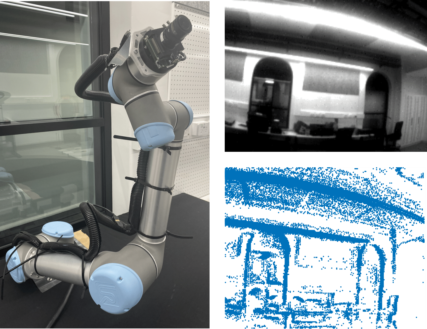
Figure 5: UR5 robot arm with DAVIS 240C event camera, and sample APS image and event image captured with our setup.

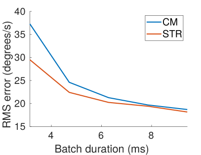
(a) Error vs batch duration $|\mathcal{T}|$.

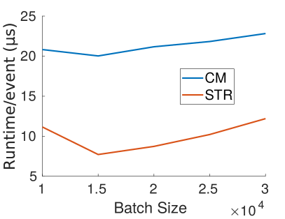
(b) Runtime vs batch size $N$.

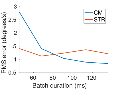
(c) Error vs batch duration $|\mathcal{T}|$.

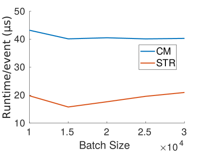
(d) Runtime vs batch size $N$.

Figure 6: RMS error (deg/s) and Runtime over batch size on boxes (top) and PureRot_Mid_On (bottom).

3.4 Results

We evaluate STR on the sequences with pure rotational motions from RobotEvt and the UZH dataset [29] (specifically poster, boxes, dynamic and shapes). All sequences have 60 s duration with ground truth orientations.

From each sequence, we extract non-overlapping consecutive event batches $\mathcal{E}$ of size $N=10,000$ to $30,000$, estimate the relative rotation $\tilde{\mathbf{R}}_{\Delta}$ from each batch and compared it against the ground truth $\mathbf{R}^{*}_{\Delta}$ using

$$d_{\angle}(\tilde{\mathbf{R}}_{\Delta},\mathbf{R}^{*}_{\Delta})=\|\log(\tilde{\mathbf{R}}_{\Delta}{\mathbf{R}^{*}_{\Delta}}^{T})\|_{2}.$$ (32)

The angular error (32) is then normalised by dividing with $\Delta$ to yield the angular velocity error (in deg/s).

We compared STR with CM [19] and EM [31]. All methods were implemented in C++ on a standard desktop with 3.0 GHz Intel i5 and 16 GB RAM. However, EM was at least two orders of magnitude slower than STR; given the large number of batches to test (e.g., $>7000$ batches in Dynamic), we leave the comparison with EM to Sec. 4.1.

Figs. 3 and 6 show the RMS angular velocity error versus batch duration $|\mathcal{T}|$ and runtime versus over batch size $N$ for PureRot_Mid_Off, boxes and PureRot_Mid_On (see supplementary material for more plots). Table 1 records the statistics on the remaining sequences of Uth (with the exception of Shapes which we show in the supplementary material due to space constraints) and sequences of RobotEvt (PureRot_Off indicates all pure rotational sequences in dark conditions; similarly for PureRot_On).

The results show that as the batch size (or equivalently batch duration in this experiment) decreases, the accuracy of CM also decreases. This trend was more pronounced in RobotEvt, possibly due to the lower (but still substantial) speeds. In contrast, STR was able to maintain accuracy throughout the event batches, which indicates a higher temporal resolution than CM. Moreover, as demonstrated in Fig. 2, STR will not suffer from increasing resolution.

PureRot_Off
Method	$10000$ ($66$ms)	$15000$ ($99$ms)	$20000$ ($133$ms)	$25000$ ($166$ms)	$30000$ ($199$ms)
STR	$\bm{2.11}$	$\bm{1.98}$	$\bm{1.91}$	$\bm{1.91}$	$\bm{2.03}$
CM [19]	$3.93$	$2.24$	$1.98$	$1.96$	$2.22$
PureRot_On
Method	$10000$ ($45$ms)	$15000$ ($68$ms)	$20000$ ($91$ms)	$25000$ ($113$ms)	$30000$ ($136$ms)
STR	$\bm{2.42}$	$\bm{2.03}$	$\bm{1.91}$	$1.9$	$2.06$
CM [19]	$13.4$	$2.57$	$2.08$	$\bm{1.91}$	$\bm{1.88}$
Dynamic
Method	$10000$ ($8$ms)	$15000$ ($12$ms)	$20000$ ($16$ms)	$25000$ ($20$ms)	$30000$ ($24$ms)
STR	$\bm{15.56}$	$\bm{13.46}$	$\bm{12.29}$	$\bm{11.69}$	$11.33$
CM [19]	$17.46$	$14.24$	$12.91$	$11.72$	$\bm{11.23}$
Poster
Method	$10000$ ($3$ms)	$15000$ ($5$ms)	$20000$ ($7$ms)	$25000$ ($8$ms)	$30000$ ($10$ms)
STR	$\bm{32.85}$	$\bm{28.36}$	$25.98$	$\bm{23.47}$	$\bm{22.30}$
CM [19]	$43.47$	$31.61$	$\bm{25.88}$	$24.57$	$23.03$

Table 1: RMS angular velocity error (deg/s) over all batches in pure rotation sequences in RobotEvt, dynamic and poster.

3.5 Utilising depth information

If depth information is available (e.g., by using stereo event cameras [49]), we show how our method can be extended to estimate full rigid (6 DoF) motion.

Assuming constant angular velocity $\bm{\omega}$ and linear velocity $\mathbf{v}$ over $\mathcal{T}$, the relative motion (3.1) between $a,b\in\mathcal{T}$ is

$$\mathbf{M}_{a,b}=\left[\begin{matrix}\mathbf{R}_{a,b}&-a\mathbf{R}_{a,b}\mathbf{v}_{a,b}+b\mathbf{v}_{a,b}\\ \mathbf{0}&1\end{matrix}\right].$$ (33)

Given two corresponding (and noiseless) events $\mathbf{e}=(\mathbf{u},d,t,p)$ and $\mathbf{e}^{\prime}=(\mathbf{u}^{\prime},d^{\prime},t^{\prime},p^{\prime})$ in $\mathcal{T}$, where $d$ and $d^{\prime}$ are respectively the depths of the events, the equation for geometric consistency in Definition 1 becomes

$$d^{\prime}\hat{\mathbf{u}}^{\prime}+t^{\prime}\mathbf{v}_{a,b}=d\mathbf{R}_{a,b}\hat{\mathbf{u}}+t\mathbf{R}_{a,b}\mathbf{v}_{a,b}.$$ (34)

See supplementary material for the justification of (34).

To estimate 6 DoF motion parameters ($\bm{\omega}_{\Delta},\mathbf{v}_{\Delta}$) from a noisy event batch $\mathcal{E}=\{\mathbf{e}_{i}\}^{N}_{i=1}=\{(\mathbf{u}_{i},z_{i},t_{i},p_{i})\}^{N}_{i=1}$ using Algorithm 1, we modify the residual (21) to become

$$r_{j}(\mathbf{R}_{\Delta},\mathbf{v}_{\Delta})=\min_{k\in\mathcal{L}_{j}}\left\|d_{k}\hat{\mathbf{u}}_{k}-d_{j}\mathbf{R}_{\Delta}\hat{\mathbf{u}}_{j}+t_{j}\mathbf{v}_{\Delta}-t_{j}\mathbf{R}_{a,b}\mathbf{v}\right\|_{2}.$$

The resulting update problem in (Step 15 in Algorithm 1)

$$\min_{\mathbf{R}_{\Delta},\mathbf{v}_{\Delta}}\sum_{j=1}^{K}r_{(j)}(\mathbf{R}_{\Delta},\mathbf{v}_{\Delta})$$ (35)

can be solved using, e.g., gradient-based optimisation such as Levenberg Marquardt. We will leave 6 DoF event-based relative motion estimation as future work.

4 Event-based visual odometry

A fundamental advantage of our relative rotation estimation method (Sec. 3) over previous techniques [19, 31, 38, 18] is that event correspondences are produced as a by-product, specifically by Step 11 in Algorithm 1. We exploit this characteristic to track features across the event stream $\mathcal{S}$ to build a rotational VO pipeline; see Algorithm 2.

Given a fixed batch size $N$, Algorithm 2 accumulates overlapping event batches with “stride” $0.5N$, i.e., if $\mathcal{E}$ and $\mathcal{E}^{\prime}$ are overlapping event batches, where

$$\mathcal{T}=[\alpha,\beta]\;\;\;\;\text{and}\;\;\;\;\mathcal{T}^{\prime}=[\alpha^{\prime},\beta^{\prime}]$$ (36)

are respectively the corresponding time windows, then $|\mathcal{E}|=N$, and $\mathcal{E}^{\prime}=N$, and the batches have in common the set of events

$$\mathcal{F}=\mathcal{E}\cap\mathcal{E}^{\prime}$$ (37)

in the time window $[\alpha^{\prime},\beta]$, where $|\mathcal{F}|=0.5N$.

To conduct tracking, without loss of generality, let $\mathcal{E}$ be the first batch. Executing Algorithm 1 (STR) on $\mathcal{E}$, we obtain the relative rotation and event correspondences

$$\mathbf{R}_{\alpha,\beta}\;\;\;\;\text{and}\;\;\;\;\{\langle\mathbf{e}_{j},\mathbf{e}_{n_{j}}\rangle\}^{K}_{j=1}.$$ (38)

Let $\bar{\mathcal{E}}$ be the subset

$$\bar{\mathcal{E}}=\{\mathbf{e}_{j},\mathbf{e}_{n_{j}}\}^{K}_{j=1}\cap\mathcal{F},$$ (39)

i.e., the subset of $\mathcal{E}$ that contains only events that make up estimated correspondences that occurred in $[\alpha^{\prime},\beta]$. Then, STR is performed on the reduced batch

$$\bar{\mathcal{E}}^{\prime}=\bar{\mathcal{E}}\cup\mathcal{E}^{\prime}\setminus\mathcal{F}$$ (40)

to estimate $\mathbf{R}_{\alpha^{\prime},\beta^{\prime}}$ and new event correspondences in $\mathcal{T}^{\prime}$; see an illustration of the process in the supplementary material. By connecting the event correspondeces in $\mathcal{T}$ and $\mathcal{T}^{\prime}$, the process generates a set of $K$ event feature tracks

$$\mathbf{e}_{i}\leftrightarrow\mathbf{e}_{j}\leftrightarrow\mathbf{e}_{k}$$ (41)

in the time window $[\alpha,\beta^{\prime}]$. By applying the same step on subsequent batches, the tracks can be extended (Step 12 in Algorithm 2). This obviates a separate feature detection and tracking heuristic [48, 4, 3, 34].

Different from Sec. 3 we set the trimming parameter $K=\lfloor 0.8|\bar{\mathcal{E}}|\rfloor$, which decreases over batches. Since sufficient features tracks are necessary to perform STR, a ”key batch” threshold $\epsilon_{k}$ is set to prevent the deficiency. If $K<\epsilon_{k}"$, the current batch $\mathcal{E}^{\prime}$ is designated a ey batch” and perform STR directly on $\mathcal{E}^{\prime}$ instead of $\bar{\mathcal{E}}^{\prime}$ and reset $K=\lfloor 0.4N\rfloor$. See Sec. 4.1 for concrete settings for $N$ and $\epsilon_{k}$.

Another crucial benefit of event feature tracking via Algorithm 1 is enabling relative rotations to be computed between event batches, and allows the construction of a pose graph $\mathcal{G}=(\mathcal{N},\mathcal{W})$, where the set of nodes

$$\mathcal{N}=\{\mathcal{E}^{(u)}\}^{U}_{u=1}$$ (42)

are event batches that share common tracked events observed thus far in the stream $\mathcal{S}$. For any two $\mathcal{E}^{(u)}$ and $\mathcal{E}^{(v)}$ with common feature tracks, we solve (23) to get the relative rotation $\mathbf{R}_{u,v}$ (see Step 14 in Algorithm 2). Given the relative rotations $\{\mathbf{R}_{u,v}\}$, a robust rotation averaging problem [10] is solved to obtain the absolute orientations $\{\mathbf{R}_{u}\}$.

Algorithm 2 Event-based rotational VO with STR.

0:  Event stream $\mathcal{S}$, camera intrinsic matrix $\mathbf{K}$, temporal threshold $\epsilon_{T}$, batch size $N$ and ”key batch” threshold $\epsilon_{k}$.

1:  $I\leftarrow 0$ and let $t_{f}$ be the duration of the event stream $\mathcal{S}$.

2:  $key\leftarrow true$, $\mathcal{N}\leftarrow empty$.

3:  $\mathcal{F}\leftarrow\{(\mathbf{u}_{i},t_{i},p_{i})\}_{i=I+1}^{I+0.5N}$.

4:  while $t_{I+0.5N}<t_{f}$ do

5:     $I\leftarrow I+0.5N$ and $K\leftarrow 0.4N$.

6:     $\mathcal{E}_{\beta}=\{(\mathbf{u}_{i},t_{i},p_{i})\}_{i=I+1}^{I+0.5N}$.

7:     if $key=true$ then $\mathcal{E}\leftarrow\mathcal{F}\cup\mathcal{E}_{\beta}$ and $\mathcal{N}\leftarrow\mathcal{F}$.

8:     else $\mathcal{E}\leftarrow\bar{\mathcal{E}}\cup\mathcal{E}_{\beta}$ and $K\leftarrow 0.8|\bar{\mathcal{E}}|$.

9:     $key\leftarrow false$ and $\mathcal{F}\leftarrow\mathcal{E}_{\beta}$.

10:     $\mathbf{R}_{\Delta},\{\langle\mathbf{e}_{j},\mathbf{e}_{n_{j}}\rangle\}_{j=1}^{K}\leftarrow$ STR($\mathcal{E}$,$\mathbf{K}$,$\epsilon_{T}$,$K$).

11:     $\bar{\mathcal{E}}=\{\mathbf{e}_{j},\mathbf{e}_{n_{j}}\}^{K}_{j=1}\cap\mathcal{F}$.

12:     $\mathcal{N}\leftarrow\mathcal{N}\cup\bar{\mathcal{E}}$.

13:     if $K>\epsilon_{k}$ then continue.

14:     $\{\mathbf{R}_{u,v}\}_{u,v\in U}\leftarrow Est\_Rot(\mathcal{E}_{u},\mathcal{E}_{v})$.

15:     $\{\mathbf{R}_{u}\}_{u\in U}\leftarrow Rot\_Avg(\{\mathbf{R}_{u,v}\}_{u,v\in U})$.

16:     $\mathcal{N}\leftarrow empty$ and $key\leftarrow true$.

17:  end while

18:  return  $\{\mathbf{R}_{u}\}$.

4.1 VO results

We benchmarked our VO technique against the following approaches on the datasets employed in Sec. 3.4:

• VCM [19]: absolute orientations were computed by chaining relative rotations from CM.

• VEM [31]: entropy maximisation method. Absolute orientations were generated by chaining.

• ZHU [48]: probabilistic feature tracking method. It’s an indirect approach (different to CM, EM and our STR), which extract and track features frrm event stream. We used the feature tracks to calculate the relative rotations, and absolute orientations were generated by chaining. For fair comparisons, we disabled the IMU input to ZHU.

We also tested our method with and without rotation averaging (VSTR${}_{\text{A}}$ and VSTR${}_{\text{C}}$). All methods operated on event batches of size $N=30,000$ for all sequences and $\epsilon_{k}=2,000$ for VSTR${}_{\text{C}}$ and VSTR${}_{\text{A}}$.

Fig. 7 plots the absolute orientation trajectories and absolute orientation error for boxes and PureRot_Fast_On, where the length of the graphs are optimised for visualisation (see supplementary material for full results). Table 2 depicts the average absolute orientation error (in deg) of each 60 s sequence and average runtime of the pipelines. VSTR achieved the best accuracy amongst most sequences and was the fastest (Note that our STR can process $1,000,000$ events/s when $N=20,000$ without sacrificing accuracy.). VEM achieved comparable accuracy but was much slower than VSTR, while VCM was slightly worse in accuracy and runtime than VSTR. The high error of ZHU indicated dependence on the IMU for tracking.

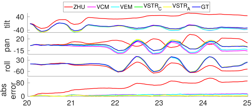
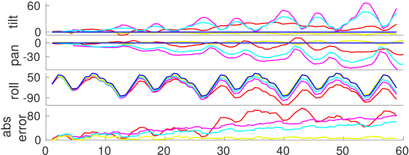
Figure 7: Absolute orientation trajectories (plotted as Euler angles) and absolute orientation error over time. Top: Poster. Bottom: PureRot_Fast_On.

Sequences	VSTR${}_{\text{C}}$	VSTR${}_{\text{A}}$	VCM	VEM	ZHU
PureRot_On	$\bm{5.11}$	$5.13$	$34.46$	$16.64$	$44.54$
PureRot_Off	$6.05$	$\bm{6.01}$	$29.38$	$7.53$	$46.76$
boxes	$11.40$	$\bm{11.38}$	$24.82$	$26.16$	$143.55$
dynamic	$21.75$	$21.78$	$26.68$	$\bm{6.36}$	$125.69$
poster	$12.97$	$\bm{12.06}$	$49.75$	$45.86$	$132.69$
Runtime (s)	$\bm{0.061}$	$0.062$	$0.538$	$2.313$	$2.863$

Table 2: Average absolute orientation error (deg) and average runtime per batch over all instances in PureRot, boxes, dynamic and poster sequences.

5 Conclusions

Accurate event-based motion estimation can be accomplished using much simpler techniques than CM, EM with less computational resources. The theoretical justification of our STR has been conducted, and the experiments showed that fewer parameters tunning are needed for different scenarios. Furthermore, the feature tracks generated by the our STR can be incorporated in solving loop closure.

References

- [1] Baker-Campbell-Hausdorff formula. https://en.wikipedia.org/wiki/Baker-Campbell-Hausdorff_formula.
- [2] Universal robots. https://www.universal-robots.com/.
- [3] Ignacio Alzugaray and Margarita Chli. Ace: An efficient asynchronous corner tracker for event cameras. In 2018 International Conference on 3D Vision (3DV), pages 653–661. IEEE, 2018.
- [4] Ignacio Alzugaray and Margarita Chli. Asynchronous corner detection and tracking for event cameras in real time. IEEE Robotics and Automation Letters, 3(4):3177–3184, 2018.
- [5] Samya Bagchi and Tat-Jun Chin. Event-based star tracking via multiresolution progressive hough transforms. In The IEEE Winter Conference on Applications of Computer Vision, pages 2143–2152, 2020.
- [6] Simon Baker and Iain Matthews. Lucas-kanade 20 years on: A unifying framework. International journal of computer vision, 56(3):221–255, 2004.
- [7] Paul J Besl and Neil D McKay. Method for registration of 3-d shapes. In Sensor fusion IV: control paradigms and data structures, volume 1611, pages 586–606. International Society for Optics and Photonics, 1992.
- [8] Jia-Wang Bian, Huangying Zhan, Naiyan Wang, Tat-Jun Chin, Chunhua Shen, and Ian Reid. Unsupervised depth learning in challenging indoor video: Weak rectification to rescue. arXiv preprint arXiv:2006.02708, 2020.
- [9] Christian Brandli, Raphael Berner, Minhao Yang, Shih-Chii Liu, and Tobi Delbruck. A 240 180 130 db 3 s latency global shutter spatiotemporal vision sensor. IEEE Journal of Solid-State Circuits, 49(10):2333–2341, 2014.
- [10] Avishek Chatterjee and Venu Madhav Govindu. Robust relative rotation averaging. IEEE transactions on pattern analysis and machine intelligence, 40(4):958–972, 2017.
- [11] Dmitry Chetverikov, Dmitry Stepanov, and Pavel Krsek. Robust euclidean alignment of 3d point sets: the trimmed iterative closest point algorithm. Image and vision computing, 23(3):299–309, 2005.
- [12] Dmitry Chetverikov, Dmitry Svirko, Dmitry Stepanov, and Pavel Krsek. The trimmed iterative closest point algorithm. In Object recognition supported by user interaction for service robots, volume 3, pages 545–548. IEEE, 2002.
- [13] Tat-Jun Chin, Samya Bagchi, Anders Eriksson, and Andre van Schaik. Star tracking using an event camera. In Proceedings of the IEEE Conference on Computer Vision and Pattern Recognition Workshops, pages 0–0, 2019.
- [14] Jörg Conradt, Matthew Cook, Raphael Berner, Patrick Lichtsteiner, Rodney J Douglas, and Tobi Delbruck. A pencil balancing robot using a pair of aer dynamic vision sensors. In 2009 IEEE International Symposium on Circuits and Systems, pages 781–784. IEEE, 2009.
- [15] Mark De Berg, Marc Van Kreveld, Mark Overmars, and Otfried Schwarzkopf. Computational geometry. In Computational geometry, pages 1–17. Springer, 1997.
- [16] Tobi Delbruck and Manuel Lang. Robotic goalie with 3 ms reaction time at 4% cpu load using event-based dynamic vision sensor. Frontiers in neuroscience, 7:223, 2013.
- [17] Guillermo Gallego, Tobi Delbruck, Garrick Orchard, Chiara Bartolozzi, Brian Taba, Andrea Censi, Stefan Leutenegger, Andrew Davison, Jörg Conradt, Kostas Daniilidis, et al. Event-based vision: A survey. arXiv preprint arXiv:1904.08405, 2019.
- [18] Guillermo Gallego, Mathias Gehrig, and Davide Scaramuzza. Focus is all you need: Loss functions for event-based vision. In Proceedings of the IEEE Conference on Computer Vision and Pattern Recognition, pages 12280–12289, 2019.
- [19] Guillermo Gallego, Henri Rebecq, and Davide Scaramuzza. A unifying contrast maximization framework for event cameras, with applications to motion, depth, and optical flow estimation. In Proceedings of the IEEE Conference on Computer Vision and Pattern Recognition, pages 3867–3876, 2018.
- [20] Guillermo Gallego and Davide Scaramuzza. Accurate angular velocity estimation with an event camera. IEEE Robotics and Automation Letters, 2(2):632–639, 2017.
- [21] Mathias Gehrig, Sumit Bam Shrestha, Daniel Mouritzen, and Davide Scaramuzza. Event-based angular velocity regression with spiking networks. arXiv preprint arXiv:2003.02790, 2020.
- [22] Arren Glover, Valentina Vasco, Massimiliano Iacono, and Chiara Bartolozzi. The event-driven Software Library for YARP — With Algorithms and iCub Applications. Frontiers in Robotics and AI, 4:73, 2018.
- [23] Hanme Kim, Stefan Leutenegger, and Andrew J Davison. Real-time 3d reconstruction and 6-dof tracking with an event camera. In European Conference on Computer Vision, pages 349–364. Springer, 2016.
- [24] Beat Kueng, Elias Mueggler, Guillermo Gallego, and Davide Scaramuzza. Low-latency visual odometry using event-based feature tracks. In 2016 IEEE/RSJ International Conference on Intelligent Robots and Systems (IROS), pages 16–23. IEEE, 2016.
- [25] Daqi Liu, Alvaro Parra, and Tat-Jun Chin. Globally optimal contrast maximisation for event-based motion estimation. In Proceedings of the IEEE/CVF Conference on Computer Vision and Pattern Recognition (CVPR), June 2020.
- [26] Elias Mueggler, Chiara Bartolozzi, and Davide Scaramuzza. Fast event-based corner detection. In British Machine Vision Conference (BMVC), number CONF, 2017.
- [27] Elias Mueggler, Christian Forster, Nathan Baumli, Guillermo Gallego, and Davide Scaramuzza. Lifetime estimation of events from dynamic vision sensors. In 2015 IEEE international conference on Robotics and Automation (ICRA), pages 4874–4881. IEEE, 2015.
- [28] Elias Mueggler, Basil Huber, and Davide Scaramuzza. Event-based, 6-dof pose tracking for high-speed maneuvers. In 2014 IEEE/RSJ International Conference on Intelligent Robots and Systems, pages 2761–2768. IEEE, 2014.
- [29] Elias Mueggler, Henri Rebecq, Guillermo Gallego, Tobi Delbruck, and Davide Scaramuzza. The event-camera dataset and simulator: Event-based data for pose estimation, visual odometry, and slam. The International Journal of Robotics Research, 36(2):142–149, 2017.
- [30] Zhenjiang Ni, Cécile Pacoret, Ryad Benosman, Siohoi Ieng, and Stéphane RÉGNIER*. Asynchronous event-based high speed vision for microparticle ing. Journal of microscopy, 245(3):236–244, 2012.
- [31] Urbano Miguel Nunes and Yiannis Demiris. Entropy minimisation framework for event-based vision model estimation. In Computer Vision – ECCV 2020, pages 161–176, Cham, 2020. Springer International Publishing.
- [32] Xin Peng, Yifu Wang, Ling Gao, and Laurent Kneip. Globally-optimal event camera motion estimation. In European Conference on Computer Vision, pages 51–67. Springer, 2020.
- [33] Henri Rebecq, Daniel Gehrig, and Davide Scaramuzza. Esim: an open event camera simulator. In Conference on Robot Learning, pages 969–982, 2018.
- [34] Henri Rebecq, Timo Horstschaefer, and Davide Scaramuzza. Real-time visual-inertial odometry for event cameras using keyframe-based nonlinear optimization. 2017.
- [35] Henri Rebecq, Timo Horstschäfer, Guillermo Gallego, and Davide Scaramuzza. Evo: A geometric approach to event-based 6-dof parallel tracking and mapping in real time. IEEE Robotics and Automation Letters, 2(2):593–600, 2016.
- [36] Hochang Seok and Jongwoo Lim. Robust feature tracking in dvs event stream using bezier mapping. In Proceedings of the IEEE/CVF Winter Conference on Applications of Computer Vision (WACV), March 2020.
- [37] Timo Stoffregen, Guillermo Gallego, Tom Drummond, Lindsay Kleeman, and Davide Scaramuzza. Event-based motion segmentation by motion compensation. In Proceedings of the IEEE/CVF International Conference on Computer Vision (ICCV), October 2019.
- [38] Timo Stoffregen and Lindsay Kleeman. Event cameras, contrast maximization and reward functions: An analysis. In The IEEE Conference on Computer Vision and Pattern Recognition (CVPR), June 2019.
- [39] David Tedaldi, Guillermo Gallego, Elias Mueggler, and Davide Scaramuzza. Feature detection and tracking with the dynamic and active-pixel vision sensor (davis). In 2016 Second International Conference on Event-based Control, Communication, and Signal Processing (EBCCSP), pages 1–7. IEEE, 2016.
- [40] Valentina Vasco, Arren Glover, and Chiara Bartolozzi. Fast event-based harris corner detection exploiting the advantages of event-driven cameras. In 2016 IEEE/RSJ International Conference on Intelligent Robots and Systems (IROS), pages 4144–4149. IEEE, 2016.
- [41] Antoni Rosinol Vidal, Henri Rebecq, Timo Horstschaefer, and Davide Scaramuzza. Ultimate slam? combining events, images, and imu for robust visual slam in hdr and high-speed scenarios. IEEE Robotics and Automation Letters, 3(2):994–1001, 2018.
- [42] Grace Wahba. A least squares estimate of satellite attitude. SIAM review, 7(3):409–409, 1965.
- [43] David Weikersdorfer, David B Adrian, Daniel Cremers, and Jörg Conradt. Event-based 3d slam with a depth-augmented dynamic vision sensor. In 2014 IEEE International Conference on Robotics and Automation (ICRA), pages 359–364. IEEE, 2014.
- [44] Chengxi Ye, Anton Mitrokhin, Cornelia Fermüller, James A Yorke, and Yiannis Aloimonos. Unsupervised learning of dense optical flow, depth and egomotion from sparse event data. arXiv preprint arXiv:1809.08625, 2018.
- [45] Huangying Zhan, Chamara Saroj Weerasekera, Jia-Wang Bian, and Ian Reid. Visual odometry revisited: What should be learnt? In 2020 IEEE International Conference on Robotics and Automation (ICRA), pages 4203–4210. IEEE, 2020.
- [46] Tinghui Zhou, Matthew Brown, Noah Snavely, and David G Lowe. Unsupervised learning of depth and ego-motion from video. In Proceedings of the IEEE Conference on Computer Vision and Pattern Recognition, pages 1851–1858, 2017.
- [47] Yi Zhou, Guillermo Gallego, and Shaojie Shen. Event-based stereo visual odometry. arXiv preprint arXiv:2007.15548, 2020.
- [48] Alex Zihao Zhu, Nikolay Atanasov, and Kostas Daniilidis. Event-based feature tracking with probabilistic data association. In 2017 IEEE International Conference on Robotics and Automation (ICRA), pages 4465–4470. IEEE, 2017.
- [49] Alex Zihao Zhu, Dinesh Thakur, Tolga Özaslan, Bernd Pfrommer, Vijay Kumar, and Kostas Daniilidis. The multivehicle stereo event camera dataset: An event camera dataset for 3d perception. IEEE Robotics and Automation Letters, 3(3):2032–2039, 2018.
- [50] Alex Zihao Zhu, Liangzhe Yuan, Kenneth Chaney, and Kostas Daniilidis. Unsupervised event-based learning of optical flow, depth, and egomotion. In Proceedings of the IEEE Conference on Computer Vision and Pattern Recognition, pages 989–997, 2019.
- [51] Alex Zihao Zhu, Nikolay Atanasov, and Kostas Daniilidis. Event-based visual inertial odometry. In Proceedings of the IEEE Conference on Computer Vision and Pattern Recognition, pages 5391–5399, 2017.