Nth Order Analytical Time Derivatives of Inverse Dynamics in Recursive and Closed Forms

Abstract

Derivatives of equations of motion describing the rigid body dynamics are becoming increasingly relevant for the robotics community and find many applications in design and control of robotic systems. Controlling robots, and multibody systems comprising elastic components in particular, not only requires smooth trajectories but also the time derivatives of the control forces/torques, hence of the equations of motion (EOM). This paper presents novel $n^{\text{th}}$ order time derivatives of the EOM in both closed and recursive forms. While the former provides a direct insight into the structure of these derivatives, the latter leads to their highly efficient implementation for large degree of freedom robotic system.

I Introduction

Rigid body dynamics algorithms and their derivatives find numerous applications in the design optimization and control of modern robotic systems. The equations of motion can be differentiated with respect to state variables, control output (generalized forces), time and physical parameters of the robot (see [17] for an overview). These derivatives can be computed by several methods: 1) approximation by finite differences, 2) automatic differentiation i.e. by applying the chain rule formula in an automatic way knowing the derivatives of basic functions (cos, sin or exp), 3) closed form symbolic derivatives of the (Lagrangian) equation of motion (EOM), and 4) recursive formulations exploiting the $O\left(n\right)$ algorithms to evaluate the EOM. While the first two methods are generic and numerical in nature, the latter two are analytical in nature and exploit the structure of the EOM.

Owing to the generality of automatic differentiation, it has been adopted by two popular optimization based control frameworks namely Drake [23] and Control Toolbox [24]. The authors in [25] argue that second-order or higher-order derivatives of the equations of motion result in very large expressions and hence find it questionable whether they should be implemented manually. However, there have been attempts in the literature [20], [19] to derive analytical and recursive partial first order derivatives of the rigid body dynamics with respect to states and generalized forces. Recently, the authors in [19] demonstrated that it is worthy to investigate efficient recursive formulations for the partial derivatives and presented computational efficiency superior to that of automatic differentiation without having to deal with costly technological setup of code generation. These derivatives are useful in optimal control of legged robots (e.g. differential dynamic programming in Crocoddyl framework [21]) and their computational design & optimization [18].

Time derivatives of the EOM are required for the control of robots with compliant joints/gears. In particular, motion planning with higher-order continuity [15] and flatness-based control of robots equipped with series elastic actuators (SEA), respectively variable stiffness actuators (VSA) [3, 5, 14] necessitate the first and second time derivatives of the equations of motion (EOM) of the robot. Therefore, recursive $O\left(n\right)$-algorithms for the evaluation of the first and second time derivatives were developed [1, 2, 6, 7, 12] extending existing $O\left(n\right)$-formulations for the evaluation of EOM. The aim of this paper is to present novel $n^{\text{th}}$ order time derivatives of equations of motion in both recursive and closed forms which can be implemented easily in any rigid body dynamics library so that they can provide time derivatives of motion equations until any order. Known applications of this work include dynamically consistent smooth motion planning with higher-order continuity [15], control of robots with flexible joints. For the subsequent treatment, the EOM are written in the form suitable for solving the inverse dynamics problem

$$\mathbf{Q}=\mathbf{M}\left(\mathbf{q}\right)\ddot{\mathbf{q}}+\mathbf{C}\left(\dot{\mathbf{q}},\mathbf{q}\right)\dot{\mathbf{q}}+\mathbf{Q}_{\mathrm{grav}}\left(\mathbf{q}\right)$$ (1)

where the vector of generalized coordinates $\mathbf{q}=\left(q_{1},\ldots,q_{n}\right)^{T}$ comprises the $n$ joint variables, $\mathbf{M}$ and $\mathbf{C}$ is the generalized mass and Coriolis matrix, respectively, and $\mathbf{Q}_{\mathrm{grav}}$ represents generalized gravity forces. Finally, $\mathbf{Q}$ are the generalized forces (drive forces/torques) required for a prescribed motion $\mathbf{q}\left(t\right)$.

Throughout the paper, we will make repeated use of the Leibniz rule for the $n^{\text{th}}$ order derivative of a product of two functions. If $f$ and $g$ are $n$ times differentiable functions, then the product $fg$ is also differentiable $n$ times and the $n^{\text{th}}$ order derivative is given by

$$(fg)^{(n)}=\sum_{k=0}^{n}{\binom{n}{k}}f^{(n-k)}g^{(k)}$$ (2)

with binomial coefficient ${\binom{n}{k}}={\frac{n!}{k!(n-k)!}}$, and $f^{(0)}\equiv f$. Here, and throughout the paper, the $n^{\text{th}}$ order derivative of $f$ is denoted with $\frac{d^{n}}{dt^{n}}f=\mathrm{D}^{(r)}f=f^{\left(n\right)}$ as appropriate.

This paper is organized as follows. Section II presents the $n^{\text{th}}$-order time derivatives of the inverse dynamics in recursive form. Section III presents the $n^{\text{th}}$-order time derivatives of the EOM in closed form. Section IV presents the application of the proposed derivatives in evaluating third order inverse dynamics of a robot manipulator and a discussion on its computational performance. Section V concludes the paper.

II Recursive $n$th-Order Inverse Dynamics Algorithm

II-A Kinematics of an open chain

A body-fixed reference frame (RFR) $\mathcal{F}_{i}$ is attached to link $i$. The configuration of body $i$ w.r.t. to a world-fixed inertia frames (IFR) is represented by a homogenous $4\times 4$ transformation matrix $\mathbf{C}_{i}\in SE\left(3\right)$ [9, 13, 16]. The configuration of body $j$ relative to body $i$ is $\mathbf{C}_{i,j}:=\mathbf{C}_{i}^{-1}\mathbf{C}_{j}$. The configuration of body $i$ is given recursively by the (local) product of exponentials (POE) as $\mathbf{C}_{i}=\ \mathbf{C}_{i-1}\mathbf{B}_{i}\exp({{}^{i}\mathbf{X}}_{i}q_{i})$. Therein, ${{}^{i}\mathbf{X}}_{i}$ is the joint screw coordinate vector in body-fixed representation, and $\mathbf{B}_{i}$ is the zero reference configuration of body $i$ and $i-1$. Notice that ${{}^{i}\mathbf{X}}_{i}$ is constant.

The twist of link $i$ in body-fixed representation is expressed by the coordinate vector [10]

$$\mathbf{V}_{i}=\left(\begin{array}[]{c}\bm{\omega}_{i}\\ \mathbf{v}_{i}\end{array}\right)$$ (3)

where $\bm{\omega}$ denotes the angular velocity of $\mathcal{F}_{i}$ relative to the world frame $\mathcal{F}_{0}$, and $\mathbf{v}$ is the translational velocity of the origin of $\mathcal{F}_{i}$ relative to $\mathcal{F}_{0}$, both resolved in $\mathcal{F}_{i}$. Denote with ${{}^{i}\mathbf{X}}_{i}$ the screw coordinate vector of joint $i$ represented in frame $\mathcal{F}_{i}$ at body $i$. The twist of link $i$, connected to its predecessor link $i-1$ by joint $i$, is

$$\mathbf{V}_{i}=\mathbf{Ad}_{\mathbf{C}_{i,i-1}}\mathbf{V}_{i-1}+{{}^{i}\mathbf{X}}_{i}\dot{q}_{i}$$ (4)

with $\mathbf{C}_{i,j}:=\mathbf{C}_{i}^{-1}\mathbf{C}_{j}$, where $\mathbf{Ad}_{\mathbf{C}_{i,i-1}}$ is the $6\times 6$ matrix transforming the twist represented in frame frame $\mathcal{F}_{i-1}$ to its representation in frame $\mathcal{F}_{i}$, and ${{}^{i}\mathbf{X}}_{i}\dot{q}_{i}$ is the relative twist of the two links due to joint $i$.

The recursive relation (4) can be summarized to yield the closed form relation

$$\mathbf{V}_{i} = \dot{q}_{1}\mathbf{B}_{i,1}+\dot{q}_{2}\mathbf{B}_{i,2}+\ldots+\dot{q}_{i}\mathbf{B}_{i,i}$$ (5)

$$= \mathbf{J}_{i}\left(\mathbf{q}\right)\dot{\mathbf{q}}$$ (6)

with the geometric Jacobian of body $i$ in body-fixed representation [10]

$$\mathbf{J}_{i}\left(\mathbf{q}\right):=\Big{(}\mathbf{B}_{i,1}\left(\mathbf{q}\right)\Big{|}\cdots\Big{|}\mathbf{B}_{i,i}\left(\mathbf{q}\right)\Big{|}\mathbf{0}\Big{|}\cdots\Big{|}\mathbf{0}\Big{)}$$ (7)

where the columns $\mathbf{B}_{i,j}$ are the instantaneous joint screws in body-fixed representation

$$\mathbf{B}_{i,j}\left(\mathbf{q}\right)=\mathbf{Ad}_{\mathbf{C}_{i,j}}\mathbf{X}_{j},\ j\leq i.$$ (8)

From its construction, follows immediately the recursive relation

$$\mathbf{B}_{i,j}=\mathbf{Ad}_{\mathbf{C}_{i,i-1}}\mathbf{B}_{i-1,j},j<i,\ \ \ \mathrm{and\ \ \ }\mathbf{B}_{i,i}=\mathbf{X}_{i}.$$ (9)

Notice that $\mathbf{B}_{i,j}$ are usually denoted with $\mathbf{J}_{i,j}$, but will not be used for sake of simplicity (avoiding the superscript). The relation

$$\dot{\mathbf{Ad}}_{\mathbf{C}_{i,i-1}}\mathbf{V}_{i-1}=\dot{q}_{i}\mathbf{ad}_{\mathbf{V}_{i}}{{}^{i}\mathbf{X}}_{i}=-\dot{q}_{i}\mathbf{ad}_{{{}^{i}\mathbf{X}}_{i}}\mathbf{V}_{i}$$ (10)

yields the recursive expression for the acceleration

$$\dot{\mathbf{V}}_{i}=\mathbf{Ad}_{\mathbf{C}_{i,i-1}}\dot{\mathbf{V}}_{i-1}+\dot{q}_{i}\mathbf{ad}_{\mathbf{V}_{i}}{{}^{i}\mathbf{X}}_{i}+{{}^{i}\mathbf{X}}_{i}\ddot{q}_{i}.$$ (11)

II-B Newton-Euler Equations of a Rigid Body

Denote with $\bm{\Theta}_{i}$ the inertia tensor of link $i$ w.r.t. its RFR $\mathcal{F}_{i}$, with $m_{i}$ the mass of link $i$, and with ${{}^{i}}\mathbf{d}_{i\text{c}}$ the distance vector from the origin of $\mathcal{F}_{i}$ to the COM of link $i$. The inertia matrix of body $i$ w.r.t. $\mathcal{F}_{i}$ is then defined as

$$\mathbf{M}_{i}=\left(\begin{array}[]{cc}\bm{\Theta}_{i}&{{}^{i}\widetilde{\mathbf{d}}}_{i\text{c}}m_{i}\\ -{{}^{i}}\widetilde{\mathbf{d}}_{i\text{c}}m_{i}&\mathbf{I}m_{i}\end{array}\right).$$ (12)

The Newton–Euler equations in body-fixed RFR $\mathcal{F}_{i}$ are

$$\mathbf{W}_{i}=\mathbf{M}_{i}\dot{\mathbf{V}}_{i}-\mathbf{ad}_{\mathbf{V}_{i}}^{T}\mathbf{M}_{i}\mathbf{V}_{i}.$$ (13)

$\mathbf{W}_{i}=(\mathbf{t}_{i},\mathbf{f}_{i})^{T}$ is the wrench applied to $\mathcal{F}_{i}$ (including gravity), where $\mathbf{t}_{i}\in{\mathbb{R}}^{3}$ is the vector of applied torques, and $\mathbf{f}_{i}\in{\mathbb{R}}^{3}$ the vector of forces applied at the origin of $\mathcal{F}_{i}$.

II-C Higher-Order Forward Kinematics

Repeated application of relation (11) yields explicit recursive relations for the jerk, jounce, etc., which were used in [12] to derive a forth-order forward kinematic and a second-order inverse dynamics algorithm. For higher-order derivatives this becomes rather involved, however. This can be avoided invoking the relations for the higher-derivative reported in [26], which are recursive in the order of derivative. To this end, introduce

$$\mathsf{B}_{i,j}(\mathbf{q},\dot{\mathbf{q}}):=\sum_{j<r\leq i}\mathbf{B}_{i,r}\left(\mathbf{q}\right)\dot{q}_{r}.$$ (14)

so that $\mathbf{V}_{i}=\mathsf{B}_{i,0}(\mathbf{q},\dot{\mathbf{q}})$. Therewith, the $k$th time derivative of the body-fixed twist is determined as

$$\mathrm{D}^{(k)}\mathbf{V}_{i}=\mathrm{D}^{(k)}\mathsf{B}_{i,0}(\mathbf{q},\dot{\mathbf{q}}).$$ (15)

The recursive relations (9) and (10) give rise to the recursive expression of time derivative of the joint screws $\mathbf{B}_{i,j}$ as

$$\dot{\mathbf{B}}_{i,j}=\sum_{j<r\leq i}\left[\mathbf{B}_{i,j},\mathbf{B}_{i,r}\right]\dot{q}_{r}=\left[\mathbf{B}_{i,j},\mathsf{B}_{i,j}\right]=\mathbf{ad}_{\mathbf{B}_{i,j}}\mathsf{B}_{i,j}.$$ (16)

Higher-order time derivatives of $\mathbf{B}_{i,j}$ are obtained for $k>0$ from (16) as

$$\mathrm{D}^{(k)}\mathbf{B}_{i,j} = \sum_{l=0}^{k-1}\tbinom{k-1}{l}[\mathrm{D}^{(l)}\mathbf{B}_{i,j},\mathrm{D}^{(k-l-1)}\mathsf{B}_{i,j}]$$

$$= \sum_{l=0}^{k-1}\tbinom{k-1}{l}\mathbf{ad}_{\mathrm{D}^{(l)}\mathbf{B}_{i,j}}\mathrm{D}^{(k-l-1)}\mathsf{B}_{i,j},\ \ j\leq i.$$

The derivatives of $\mathsf{B}_{i,j}$ follow with (14) simply as

$$\mathrm{D}^{(k)}\mathsf{B}_{i,j}=\sum_{j<r\leq i}\sum_{l=0}^{k}\tbinom{k}{l}\mathrm{D}^{(l)}\mathbf{B}_{i,r}q_{r}^{(k-l+1)}.$$ (18)

The important point is that these relations can be easily implemented. The explicit third- and forth-order relations reported in [12] are special cases, where the recursive relations (II-C) and (18) are rolled out.

II-D Inverse Dynamics

The backward recursion step in the (standard) inverse dynamics algorithm, in terms of body-fixed twists and wrenches, [12] is

$$\mathbf{W}_{i}=\mathbf{Ad}_{\mathbf{C}_{i+1,i}}^{T}\mathbf{W}_{i+1}+\mathbf{M}_{i}\dot{\mathbf{V}}_{i}-\mathbf{ad}_{\mathbf{V}_{i}}^{T}\mathbf{M}_{i}\mathbf{V}_{i}.$$ (19)

Higher-order derivatives of the backward recursion step (19) follow with Leibniz’ rule (2) as

$$\mathrm{D}^{(k)}\mathbf{W}_{i} = \sum_{r=0}^{k}\tbinom{k}{r}\mathrm{D}^{(r)}\mathbf{Ad}_{\mathbf{C}_{i+1,i}}^{T}\mathrm{D}^{(k-r)}\mathbf{W}_{i+1}$$

$$+\mathbf{M}_{i}\mathrm{D}^{(k)}\mathbf{V}_{i}-\sum_{r=0}^{k}\tbinom{k}{r}\mathbf{ad}_{\mathrm{D}^{(r)}\mathbf{V}_{i}}^{T}\mathbf{M}_{i}\mathrm{D}^{(k-r)}\mathbf{V}_{i}.$$

The relation $\dot{\mathbf{Ad}}_{\mathbf{C}_{i+1,i}}=-\dot{q}_{i+1}\mathbf{ad}_{{{}^{i+1}\mathbf{X}}_{i+1}}\mathbf{Ad}_{\mathbf{C}_{i+1,i}}$ gives rise to

$$\mathrm{D}^{(k)}\mathbf{Ad}_{\mathbf{C}_{i+1,i}}=-\mathbf{ad}_{{{}^{i+1}\mathbf{X}}_{i+1}}\sum_{r=0}^{k-1}\tbinom{k-1}{r}\mathrm{D}^{(r)}\mathbf{Ad}_{\mathbf{C}_{i+1,i}}q_{i+1}^{(k-r)}$$

which allows evaluating (II-D).

II-E Higher-Order Inverse Dynamics Algorithm

$k$th-Order Forward Kinematics

• Input: $\mathbf{q},\dot{\mathbf{q}},\ddot{\mathbf{q}},\ldots,\mathbf{q}^{\left(k\right)}$

• Preparation run (computation of basic kinematic data)

  • For body $i=1$:

    $$\mathbf{C}_{1} = \mathbf{B}_{1}\exp({{}^{1}\mathbf{X}}_{1}q_{1})$$

    $$\mathbf{B}_{1,1} = {{}^{1}\mathbf{X}}_{1},\ \mathsf{B}_{1,1}=\ {{}^{1}\mathbf{X}}_{1}\dot{q}_{i}$$

  • For $i=2,\ldots,n$ (recursion over bodies)

    $$\mathbf{C}_{i} = \mathbf{C}_{i-1}\mathbf{B}_{i}\exp({{}^{i}\mathbf{X}}_{i}q_{i})$$

    $$\mathbf{C}_{i,i-1} = \mathbf{C}_{i}^{-1}\mathbf{C}_{i-1}$$

    $$\mathbf{B}_{i,j} = \mathbf{Ad}_{\mathbf{C}_{i,i-1}}\mathbf{B}_{i-1,j},\ j=1,\ldots,i$$

    End

• For $r=0,\ldots,k$ (recursion over order of derivative)

  • For body $i=1$:

    $$\mathrm{D}^{(r)}\mathbf{V}_{1} = {{}^{1}\mathbf{X}}_{1}q^{\left(r+1\right)}$$

    $$\mathrm{D}^{(r)}\mathbf{B}_{1,1} = \mathbf{0},\ r\geq 1$$

  • For $i=2,\ldots,n$ (recursion over bodies)

    $$\mathrm{D}^{(k)}\mathbf{Ad}_{\mathbf{C}_{i,i-1}}=-\mathbf{ad}_{{{}^{i}\mathbf{X}}_{i}}\sum_{r=0}^{k-1}\tbinom{k-1}{r}\mathrm{D}^{(r)}\mathbf{Ad}_{\mathbf{C}_{i,i-1}}q_{i}^{(k-r)}$$

    • For $j=i,i-1.\ldots,1$

      $$\mathrm{D}^{(r)}\mathbf{B}_{i,j} =\sum_{l=0}^{r-1}\tbinom{r-1}{l}\mathbf{ad}_{\mathrm{D}^{(l)}\mathbf{B}_{i,j}}\mathrm{D}^{(r-l-1)}\mathsf{B}_{i,j},r>1$$

      $$\mathrm{D}^{(r)}\mathsf{B}_{i,j} =\sum_{j\leq k\leq i}\sum_{l=0}^{r}\tbinom{r}{l}\mathrm{D}^{(l)}\mathbf{B}_{i,r}q_{j}^{(r-l+1)}$$

      $$\mathrm{D}^{(r)}\mathbf{V}_{i} =\mathrm{D}^{(r)}\mathsf{B}_{i,1}(\mathbf{q},\dot{\mathbf{q}})$$

      end

    end

  end

• Output: $\mathbf{C}_{i},\mathrm{D}^{(k)}\mathbf{V}_{i},\mathrm{D}^{(k)}\mathbf{B}_{i,j},\mathrm{D}^{(k)}\mathsf{B}_{i,j}$

$k$th-Order Inverse Dynamics

• Input: $\mathbf{C}_{i},\mathrm{D}^{(k)}\mathbf{V}_{i}^{\mathrm{b}}$

• For $i=n-1,\ldots,1$

$$\mathrm{D}^{(k)}\mathbf{W}_{i} = \sum_{r=0}^{k}\tbinom{k}{r}\mathrm{D}^{(r)}\mathbf{Ad}_{\mathbf{C}_{i+1,i}}^{T}\mathrm{D}^{(k-r)}\mathbf{W}_{i+1}$$

$$+\mathbf{M}_{i}^{\text{b}}\mathrm{D}^{(k)}\mathbf{V}_{i}$$

$$-\sum_{r=0}^{k}\tbinom{k}{r}\mathbf{ad}_{\mathrm{D}^{(r)}\mathbf{V}_{i}}^{T}\mathbf{M}_{i}\mathrm{D}^{(k-r)}\mathbf{V}_{i}$$

$$\mathrm{D}^{(k)}Q_{i} = {{}^{i}\mathbf{X}}_{i}^{T}\mathrm{D}^{(k)}\mathbf{W}_{i}$$

end

• Output: $\mathrm{D}^{(k)}\mathbf{Q}$

III $n$th-Order Time Derivatives of Equations of Motion

III-A EOM in Closed Form

The individual twists of all bodies are summarized in the vector $\mathsf{V}\in{\mathbb{R}}^{6n}$, which is referred to as the system twist in body-fixed representation. It is determined as

$$\mathsf{V}=\mathsf{J}\dot{\mathbf{q}}$$ (21)

with the system Jacobian $\mathsf{J}\left(\mathbf{q}\right)$. The latter admits the factorization

$$\mathsf{J}=\mathsf{AX}$$ (22)

in terms of the block-triangular and block-diagonal matrices

$$\mathsf{A}\left(\mathbf{q}\right) = \left(\begin{array}[]{ccccc}\mathbf{I}&\mathbf{0}&\mathbf{0}&&\mathbf{0}\\ \mathbf{Ad}_{\mathbf{C}_{2,1}}&\mathbf{I}&\mathbf{0}&\cdots&\mathbf{0}\\ \mathbf{Ad}_{\mathbf{C}_{3,1}}&\mathbf{Ad}_{\mathbf{C}_{3,2}}&\mathbf{I}&&\mathbf{0}\\ \vdots&\vdots&\ddots&\ddots&\\ \mathbf{Ad}_{\mathbf{C}_{n,1}}&\mathbf{Ad}_{\mathbf{C}_{n,2}}&\cdots&\mathbf{Ad}_{\mathbf{C}_{n,n-1}}&\mathbf{I}\end{array}\right)$$ (28)

$$\mathsf{X} = \left(\begin{array}[]{ccccc}{{}^{1}\mathbf{X}}_{1}&\mathbf{0}&\mathbf{0}&&\mathbf{0}\\ \mathbf{0}&{{}^{2}\mathbf{X}}_{2}&\mathbf{0}&\cdots&\mathbf{0}\\ \mathbf{0}&\mathbf{0}&{{}^{3}\mathbf{X}}_{3}&&\mathbf{0}\\ \vdots&\vdots&\ddots&\ddots&\\ \mathbf{0}&\mathbf{0}&\cdots&\mathbf{0}&{{}^{n}}\mathbf{X}_{n}\end{array}\right)$$ (34)

where ${{}^{i}\mathbf{X}}_{i}$ is the screw coordinate vector associated to joint $i$ represented in the body-frame of body $i$. The vectors ${{}^{i}\mathbf{X}}_{i}$ are constant due to the body-fixed representation. The matrix $\mathbf{Ad}_{\mathbf{C}_{i,j}}$ transforms screw coordinates represented in the reference frame at body $j$ to those represented in the frame on body $i$ [9, 13, 16]. A central relation for deriving the EOM in closed form is the following expression for the time derivative of the matrix $\mathsf{A}$ and thus of the system Jacobian [10]

$$\dot{\mathsf{J}}\left(\mathbf{q},\dot{\mathbf{q}}\right)=-\mathsf{A}\left(\mathbf{q}\right)\mathsf{a}\left(\dot{\mathbf{q}}\right)\mathsf{J}\left(\mathbf{q}\right)$$ (35)

where

$$\mathsf{a}\left(\dot{\mathbf{q}}\right)=\mathrm{diag}~{}(\dot{q}_{1}\mathbf{ad}_{{{{}^{1}}\mathbf{X}_{1}}},\ldots,\dot{q}_{n}\mathbf{ad}_{{{{}^{n}}\mathbf{X}_{n}}}).$$ (36)

This gives rise to the closed form expressions for the system acceleration

$$\dot{\mathsf{V}}=\mathsf{J}\ddot{\mathbf{q}}-\mathsf{AaJ}\dot{\mathbf{q}}=\mathsf{J}\ddot{\mathbf{q}}-\mathsf{AaV}.$$ (37)

For calculating the derivatives, the time derivative of matrix $\mathsf{A}$ will be needed. It can be shown that the derivative of $\mathsf{A}$ is [10]

$$\dot{\mathsf{A}}\left(\mathbf{q},\dot{\mathbf{q}}\right)=\mathsf{A}\left(\mathbf{q}\right)\mathsf{a}-\mathsf{A}\left(\mathbf{q}\right)\mathsf{a}\left(\dot{\mathbf{q}}\right)\mathsf{A}\left(\mathbf{q}\right).$$ (38)

Clearly, the derivative (35) of the system Jacobian is recovered as $\dot{\mathsf{J}}=\dot{\mathsf{A}}\mathsf{X}$ noting that $\mathsf{aX}\equiv\mathbf{0}$.

The generalized mass and Coriolis matrix in the EOM (1) of a simple kinematic chain mounted at the ground are found via Jourdain’s principle of virtual power as (or likewise as the Lagrange equations) [10]

$$\mathbf{M}\left(\mathbf{q}\right)=\mathsf{J}^{T}\mathsf{MJ,\ \ \ \ }\mathbf{C}\left(\mathbf{q},\dot{\mathbf{q}}\right)=\mathsf{J}^{T}\mathsf{CJ}$$ (39)

where

$$\mathsf{M} := \mathrm{diag}\,(\mathbf{M}_{1},\ldots,\mathbf{M}_{n})$$ (40)

$$\mathsf{C}(\mathbf{q},\dot{\mathbf{q}},\mathsf{V}\left(\dot{\mathbf{q}}\right)) := -\mathsf{MAa}-\mathsf{b}^{T}\mathsf{M}.$$ (41)

Therein, $\mathbf{M}_{i}$ is the (constant) $6\times 6$ inertia matrix of body $i$ expressed in the body-frame, and

$$\mathsf{b}\left(\mathsf{V}\right):=\mathrm{diag}~{}(\mathbf{ad}_{\mathbf{V}_{1}},\ldots,\mathbf{ad}_{\mathbf{V}_{n}}).$$ (42)

A closed form of the EOM is obtained after replacing the system twist by (21). Alternatively, first the kinematic relation (21) and then the coefficient matrices in (41) are evaluated for a given state $\mathbf{q},\dot{\mathbf{q}}$. The generalized gravity forces are given as

$$\mathbf{Q}_{\mathrm{grav}}\left(\mathbf{q}\right)=\mathsf{J}^{T}\mathsf{MU}\dot{\mathbf{V}}_{0}$$ (43)

with

$$\dot{\mathbf{V}}_{0}=\left(\begin{array}[]{c}\mathbf{0}\\ {}^{0}\mathbf{g}\end{array}\right),\mathsf{U}\left(\mathbf{q}\right)=\mathsf{A}\left(\begin{array}[]{c}\mathbf{I}\\ \mathbf{0}\\ \vdots\\ \mathbf{0}\end{array}\right)=\left(\begin{array}[]{c}\mathbf{Ad}_{\mathbf{C}_{1}}^{-1}\\ \mathbf{Ad}_{\mathbf{C}_{2}}^{-1}\\ \vdots\\ \mathbf{Ad}_{\mathbf{C}_{n}}^{-1}\end{array}\right).$$ (44)

Here, ${}^{0}\mathbf{g}$ is the vector of gravitational acceleration expressed in the inertial frame, which is transformed to the individual bodies by $\mathsf{U}$.

III-B Higher-Order Time Derivatives of the EOM

In this section, the expressions for $n^{\text{th}}$ order time derivatives of the EOM in closed form are derived. Applying Leibniz’s rule (2) on the EOM (1), one gets

$$\mathbf{Q}^{(n)} = \sum_{k=0}^{n}{\binom{n}{k}}\mathbf{M}^{(n-k)}\ddot{\mathbf{q}}^{(k)}+$$

$$\sum_{k=0}^{n}{\binom{n}{k}}\mathbf{C}^{(n-k)}\dot{\mathbf{q}}^{(k)}+\mathbf{Q}_{\mathrm{grav}}^{(n)}$$

which in an expanded form can also be written as

$$\mathbf{Q}^{(n)}-\mathbf{Q}_{\mathrm{grav}}^{(n)} =\mathbf{M}\ddot{\mathbf{q}}^{(n)}+(n\mathbf{M}^{(1)}+\mathbf{C})\ddot{\mathbf{q}}^{(n-1)}+\ldots$$

$$+\left[{\binom{n}{k}}\mathbf{M}^{(n-k)}+{\binom{n}{k+1}}\mathbf{C}^{(n-k-1)}\right]\ddot{\mathbf{q}}^{(k)}$$

$$+\left[{\binom{n}{k-1}}\mathbf{M}^{(n-k+1)}+{\binom{n}{k}}\mathbf{C}^{(n-k)}\right]\dot{\mathbf{q}}^{(k)}$$

$$+\ldots+(\mathbf{M}^{(n)}+n\mathbf{C}^{(n-1)})\ddot{\mathbf{q}}+\mathbf{C}^{(n)}\dot{\mathbf{q}}.$$

One can arrive at first order and second order time derivative of EOM by substituting $n=1$ and $n=2$ in (III-B) respectively

$$\dot{\mathbf{Q}} =\mathbf{M}\dddot{\mathbf{q}}+(\dot{\mathbf{M}}+\mathbf{C})\ddot{\mathbf{q}}+\dot{\mathbf{C}}\dot{\mathbf{q}}+\dot{\mathbf{Q}}_{\mathrm{grav}}$$ (46)

$$\ddot{\mathbf{Q}} =\mathbf{M}\ddot{\ddot{\mathbf{q}}}+(2\dot{\mathbf{M}}+\mathbf{C})\dddot{\mathbf{q}}+(\ddot{\mathbf{M}}+2\dot{\mathbf{C}})\ddot{\mathbf{q}}+\ddot{\mathbf{C}}\dot{\mathbf{q}}+\ddot{\mathbf{Q}}_{\text{grav}}$$ (47)

The matrix coefficient $\mathbf{P}_{k}$ of $k^{\text{th}}$ derivative of $\mathbf{q}$ in the $n^{\text{th}}$ order time derivative of the EOM expressed as

$$\mathbf{Q}^{(n)}-\mathbf{Q}_{\mathrm{grav}}^{(n)}=\mathbf{M}\mathbf{q}^{(n+2)}+\ldots+\mathbf{P}_{k}\mathbf{q}^{(k)}+$$ (48)

$$\ldots+\mathbf{C}^{(n)}\mathbf{q}^{(1)}$$

is given by

$$\mathbf{P}_{k}={\binom{n}{k-2}}\mathbf{M}^{(n-k+2)}+{\binom{n}{k-1}}\mathbf{C}^{(n-k+1)}$$ (49)

for all $2\leq k\leq n+1,n\geq 1$. For example, the matrix coefficient of $\mathbf{q}^{(3)}$ in $2^{\text{nd}}$ order time derivatives of the EOM can be computed by substituting $k=3,n=2$ in (49) as $(2\dot{\mathbf{M}}+\mathbf{C})$ which can be verified from (47). In the following, higher order derivatives of various kinematic and dynamic quantities are presented which are needed in evaluating higher order derivatives of the generalized forces in (48).

III-B1 Higher Order Kinematics

For all $n\geq 1$, the $n^{\text{th}}$ order time derivative of the matrix $\mathsf{A}$ can be expressed as

$$\mathsf{A}^{(n)}=\sum_{k=0}^{n-1}{\binom{n-1}{k}}\mathsf{A}^{(n-1-k)}\mathsf{a}^{(k)}-$$ (50)

$$\sum_{k=0}^{n-1}{\binom{n-1}{k}}\mathsf{A}^{(n-1-k)}\sum_{j=0}^{k}{\binom{k}{j}}\mathsf{a}^{(k-j)}\mathsf{A}^{(j)}.$$

which requires the higher order derivatives of the matrix $\mathsf{a}$. The $n^{\text{th}}$ order time derivative of the matrix $\mathsf{a}$ is given by

$$\mathsf{a}^{\left(n\right)}\left(\mathbf{q}^{\left(n\right)}\right)=\mathrm{diag}~{}(q^{\left(n\right)}_{1}\mathbf{ad}_{{{{}^{1}}\mathbf{X}_{1}}},\ldots,q^{\left(n\right)}_{n}\mathbf{ad}_{{{{}^{n}}\mathbf{X}_{n}}}).$$ (51)

By performing a book keeping of all the previous derivatives of $\mathsf{A}$ and $\mathsf{a}$, $n^{\text{th}}$ derivative of the matrix $\mathsf{A}$ can be easily computed.

Using the (50) and (22), $n^{\text{th}}$ time derivative of the system level Jacobian matrix can be computed as

$$\mathsf{J}^{(n)}=\mathsf{A}^{(n)}\mathsf{X}.$$ (52)

Similarly, $n^{\text{th}}$ time derivative of the system velocities can be obtained via

$$\mathsf{V}^{(n)}=\sum_{k=0}^{n}{\binom{n}{k}}\mathsf{J}^{(n-k)}\dot{\mathbf{q}}^{(k)}.$$ (53)

III-B2 Higher Order Mass-Inertia matrix

The $n^{\text{th}}$ time derivative of the mass-inertia matrix $\mathbf{M}$ is given by

$$\mathbf{M}^{(n)}=\sum_{k=0}^{n}{\binom{n}{k}}{\mathsf{J}}^{(n-k)T}\mathsf{M}{\mathsf{J}}^{(k)}$$ (54)

which could be readily computed using higher order derivatives of the system level Jacobian (52).

III-B3 Higher Order Coriolis-Centrifugal Matrix

The $n^{\text{th}}$ time derivative of the Coriolis-Centrifugal matrix $\mathbf{C}$ is given by:

$$\mathbf{C}^{(n)}=\sum_{k=0}^{n}{\binom{n}{k}}{\mathsf{J}}^{(n-k)T}\sum_{j=0}^{k}{\binom{k}{j}}\mathsf{C}^{(k-j)}{\mathsf{J}}^{(j)}$$ (55)

which necessities the higher order derivatives of $\mathsf{C}$. The expression of $n^{\text{th}}$ time derivative of system level Coriolis-Centrifugal matrix is given by

$$\mathsf{C}^{(n)}=-\mathsf{M}\sum_{k=0}^{n}{\binom{n}{k}}{\mathsf{A}}^{(n-k)}{\mathsf{a}}^{(k)}-\mathsf{b}^{(n)T}{\mathsf{M}}$$ (56)

which requires the $n^{\text{th}}$ order derivative of the matrix $\mathsf{b}$ computed as

$$\mathsf{b}^{\left(n\right)}\left(\mathsf{V}^{\left(n\right)}\right):=\mathrm{diag}~{}\left(\mathbf{ad}_{\mathbf{V}_{1}^{\left(n\right)}},\ldots,\mathbf{ad}_{\mathbf{V}_{n}^{\left(n\right)}}\right)$$ (57)

and higher order derivatives of $\mathsf{A}$ and $\mathsf{a}$ available in (50) and (51) respectively.

III-B4 Higher Order Gravity Force Vector

The $n^{\text{th}}$ order time derivative of the vector of gravity forces $\mathbf{Q}_{\text{grav}}$ is given by

$$\mathbf{Q}_{\text{grav}}^{(n)}=\sum_{k=0}^{n}{\binom{n}{k}}{\mathsf{J}}^{(n-k)T}\mathsf{M}\mathsf{A}^{\left(k\right)}\left(\begin{array}[]{c}\mathbf{I}\\ \mathbf{0}\\ \vdots\\ \mathbf{0}\end{array}\right)\dot{\mathbf{V}}_{0}.$$ (58)

IV Results and Discussion

The $n^{\text{th}}$ order recursive inverse dynamics algorithm presented in Section II and higher order closed form equations of motion presented in Section III were implemented in MATLAB. This section presents their application to the computation of higher order inverse dynamics of a robot manipulator and presents a discussion on their computational efficiency.

IV-A Example: Third Order Inverse Dynamics

Both algorithms are applied to compute the third order inverse dynamics of a six degrees of freedom (DOF) Franka Emika Panda robot as shown in Figure 1 (left). Using the geometric information provided in Figure 1, it is straight-forward to deduce the joint screw coordinate vectors ${}^{i}\mathbf{X}_{i}$ and the relative reference configuration of all the links $\mathbf{B}_{i}$ thanks to the simplicity of this modeling approach as compared to the DH parameters (for details see [11]). The mass–inertia data w.r.t. the RFRs was determined as reported in [28] providing the body-fixed link mass matrices (12). Due to space the limitation, details are omitted here. The joint trajectory, taking from [28], as shown in Figure 1 (right) is used as the input motion trajectory for the system and the inverse dynamics of the manipulator arm is computed up to $3^{\text{rd}}$ order. Figure 2, 3, 4 and 5 show the higher order inverse dynamics results (i.e. $\mathbf{Q}(t),\dot{\mathbf{Q}}(t),\ddot{\mathbf{Q}}(t),\dddot{\mathbf{Q}}(t)$). The results were verified with numerical differentiation of the generalized forces. Both recursive and closed form algorithms indeed yield the same solution of the higher-order forward kinematics and inverse dynamics problem (within the numerical accuracy).

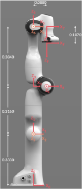
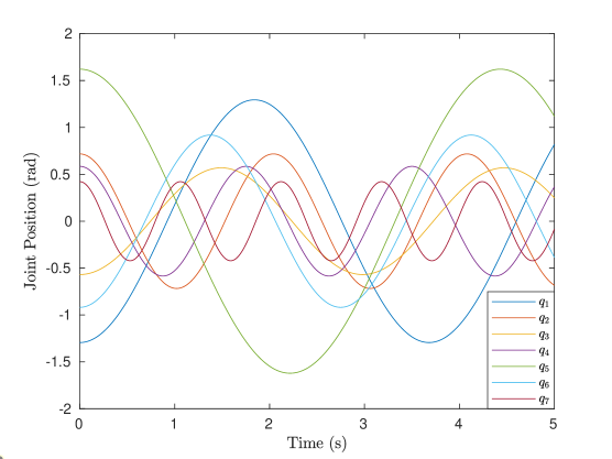
Figure 1: Franka Emika Panda robot with geometric parameters in the zero configuration (i.e. $\mathbf{q}=0$) (left) and input joint motion trajectory (right)

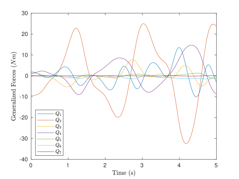
Figure 2: Inverse Dynamics

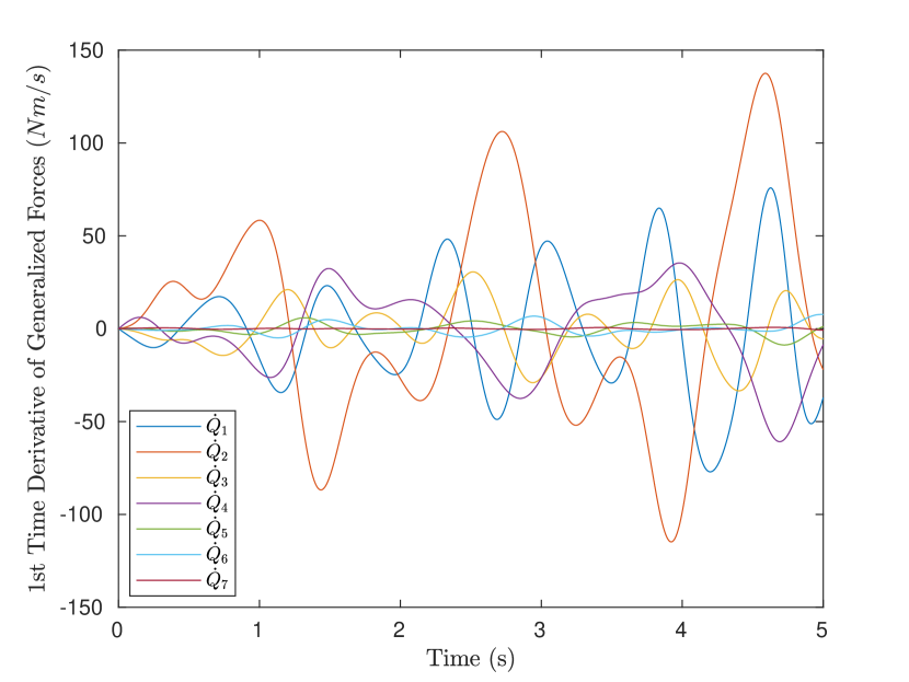
Figure 3: 1st Order Inverse Dynamics

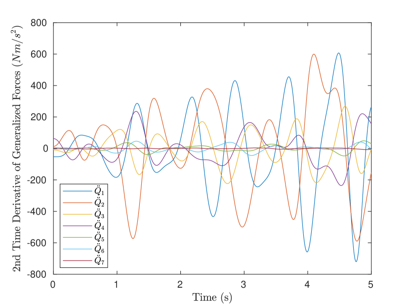
Figure 4: 2nd Order Inverse Dynamics

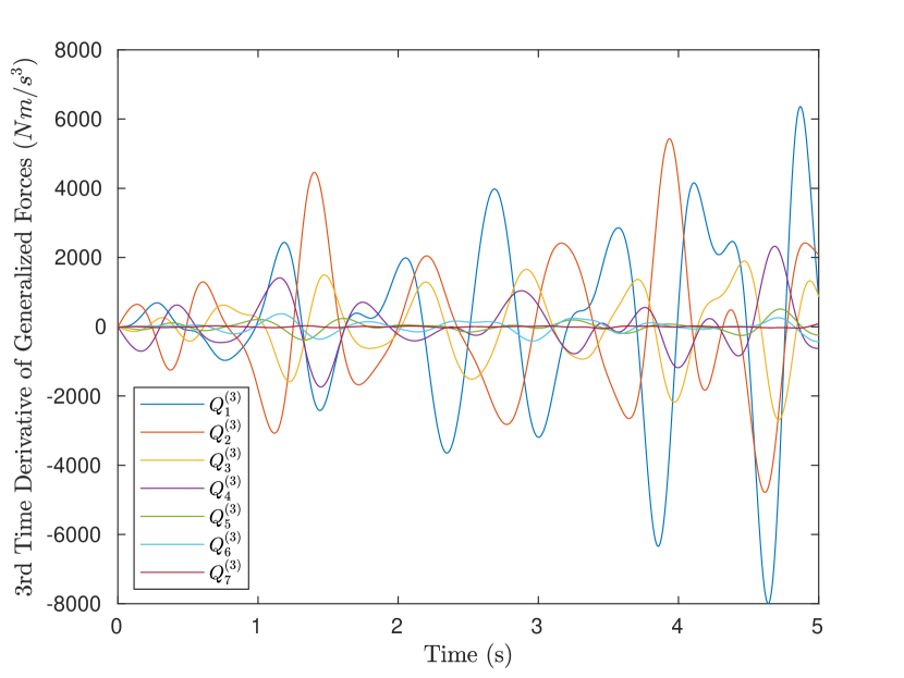
Figure 5: 3rd Order Inverse Dynamics

IV-B Discussion on Computational Performance

The computational performance of the recursive and closed form algorithms was evaluated by measuring the total CPU time spent in $10000$ evaluations of $2^{\text{nd}}$ order inverse dynamics on a standard laptop with Intel Core i7-6600U CPU clocked at 2.6 GHz and 16 GB RAM. It was found that $n^{\text{th}}$ order recursive algorithm takes $117$ seconds and the $n^{\text{th}}$ order closed form algorithm takes a total of $124$ seconds for $10000$ calls. Hence, it can be noticed that the recursive version of the algorithm slightly outperforms the closed form version of the algorithm as expected. It is to be noted that the closed form expressions were implemented using usual matrices in MATLAB and computational performance can be improved by exploiting the sparse matrix algebra. In both cases, the equations were implemented without any optimization, e.g. avoiding multiplication with zeros etc. These computation times are only preliminary indicators and will reduce in an optimized C++ implementation.

Additionally, we investigated how the computational efficiency of these general purpose algorithms for $n^{\text{th}}$ order derivatives compares to the hand–crafted recursive [12] and closed form algorithms [29] for $2^{\text{nd}}$ order inverse dynamics based on our previous work. It was found that these hand–crafted algorithms for $2^{\text{nd}}$ inverse dynamics are faster than $n^{\text{th}}$ order algorithms with $n=2$. For example, the recursive $2^{\text{nd}}$ order inverse dynamics algorithm requires only $24$ seconds and the corresponding closed form version requires $69$ seconds for $10000$ evaluations. Apparently, the generality of these algorithms comes at some computational expense which we believe is justified for the benefit that they admit evaluating derivative of any order without the need to derive them by hand or with automatic differentiation tools. This seems even justified for specific applications, where one would use a hand–crafted algorithm, given the low runtime and the potential for performance improvement when efficiently implemented. The presented algorithms can also complement and improve the functionality of rigid body dynamics libraries.

V Conclusion

This paper presents novel recursive and closed form expressions for the $n^{\text{th}}$ order time derivative of the EOM of a kinematic chain. Building upon the Lie formulation of the EOM the formulations are advantageous as they are expressed in terms of joint screw coordinates, and thus facilitate parameterization in terms of vector quantities that can be easily obtained. With these relations, general geometric formulations for the $n^{\text{th}}$ order time derivatives as needed for motion planning and control are now available. Future research will also address the $n^{\text{th}}$ order time derivatives of general mechanisms with kinematic loops and an efficient C++ based implementation in Hybrid Robot Dynamics (HyRoDyn) software framework [27].

References

• [1] G. Buondonno, A. De Luca: A recursive Newton-Euler algorithm for robots with elastic joints and its application to control, 2015 IEEE/RSJ IROS, 5526-5532
• [2] G. Buondonno, A. De Luca: Efficient Computation of Inverse Dynamics and Feedback Linearization for VSA-Based Robots, IEEE Rob. Aut. Letters, 1(2), 2016, 908-915
• [3] A. De Luca: Decoupling and feedback linearization of robots with mixed rigid/elastic joints, Int. J. Rob. Nonlin. Cont., 8, 1998, 965-977
• [4] R. Featherstone: Rigid Body Dynamics Algorithms, Springer, 2008
• [5] H. Gattringer, et al.: Recursive methods in control of flexible joint manipulators, Multibody Syst Dyn. 32, 2014, 117-131
• [6] C. Guarino Lo Bianco, E. Fantini: A recursive Newton-Euler approach for the evaluation of generalized forces derivatives, 12th IEEE Int. Conf. Methods Models Autom. Robot., 2006, 739-744
• [7] C. Guarino Lo Bianco: Evaluation of Generalized Force Derivatives by Means of a Recursive Newtonโ€“Euler Approach, IEEE Trans. Rob., 25(4), 954-959
• [8] A. Jain: Robot and Multibody Dynamics, Springer Science+Business Media, 2011
• [9] K.M. Lynch, F.C. Park: Modern Robotics, Cambridge, 2017
• [10] A. Mรผller: Screw and Lie group theory in multibody dynamics โ€“ Recursive algorithms and equations of motion of tree-topology systems, Multibody System Dynamics, 42(2), 2018 219-248
• [11] Mรผller, A. Screw and Lie group theory in multibody kinematics. Multibody Syst Dyn 43, 37-70 (2018). https://doi.org/10.1007/s11044-017-9582-7
• [12] A. Mรผller: Recursive Second-Order Inverse Dynamics for Serial Manipulators, IEEE Int. Conf. Robotics Automations (ICRA), May 29-June 3, 2017, Singapore
• [13] R.M. Murray, Z. Li, and S.S. Sastry, A Mathematical Introduction to Robotic Manipulation, CRC Press BocaRaton, 1994
• [14] G. Palli, C. Melchiorri, A. De Luca: On the Feedback Linearization of Robots with Variable Joint Stiffness, IEEE Int. Conf. Rob. Aut. (IROS), Pasadena, CA, USA, May 19-23, 2008
• [15] A. Reiter, A. Mรผller, H. Gattringer: On Higher-Order Inverse Kinematics Methods in Time-Optimal Trajectory Planning for Kinematically Redundant Manipulators, IEEE Trans. Industrial Informatics, Vol. 14, No. 4, 2018, pp. 1681 - 1690
• [16] J. Selig: Geometric Fundamentals of Robotics (Monographs in Computer Science Series), Springer-Verlag New York, 2005
• [17] G. Garofalo, C. Ott, A. Albu-Schรคffer: On the closed form computation of the dynamic matrices and their differentiations, 2013 IEEE/RSJ International Conference on Intelligent Robots and Systems, Tokyo, 2013, pp. 2364-2359.
• [18] Ha, Sehoon, Stelian Coros, Alexander Alspach, Joohyung Kim, and Katsu Yamane. โ€Joint Optimization of Robot Design and Motion Parameters using the Implicit Function Theorem.โ€ In Robotics: Science and Systems. 2017.
• [19] Carpentier, Justin, and Nicolas Mansard. โ€Analytical derivatives of rigid body dynamics algorithms.โ€ In Robotics: Science and Systems. 2018.
• [20] Sung-Hee Lee, Junggon Kim, F. C. Park, Munsang Kim and J. E. Bobrow, โ€Newton-type algorithms for dynamics-based robot movement optimization,โ€ In IEEE Transactions on Robotics, vol. 21, no. 4, pp. 657-667, Aug. 2005.
• [21] Mastalli, Carlos, Rohan Budhiraja, Wolfgang Merkt, Guilhem Saurel, Bilal Hammoud, Maximilien Naveau, Justin Carpentier, Sethu Vijayakumar, and Nicolas Mansard. โ€Crocoddyl: An Efficient and Versatile Framework for Multi-Contact Optimal Control.โ€ arXiv preprint arXiv:1909.04947 (2019).
• [22] Kumar, Shivesh. โ€Modular and Analytical Methods for Solving Kinematics and Dynamics of Series-Parallel Hybrid Robots.โ€ PhD diss., Universitรคt Bremen, 2019
• [23] Russ Tedrake and the Drake Development Team. โ€Drake: Model-based design and verification for robotics.โ€ url = โ€https://drake.mit.eduโ€, 2019
• [24] Markus Giftthaler, Michael Neunert, Markus Stรคuble, Jonas Buchli. โ€The control toolbox An open-source C++ library for robotics, optimal and model predictive control.โ€ 2018 IEEE International Conference on Simulation, Modeling, and Programming for Autonomous Robots (SIMPAR), pp. 123-129, 2018.
• [25] Markus Giftthaler, Michael Neunert, Markus Stรคuble, Marco Frigerio, Claudio Semini, Jonas Buchli. โ€Automatic Differentiation of Rigid Body Dynamics for Optimal Control and Estimation.โ€ Advanced Robotics, 31:22, 1225-1237, DOI: 10.1080/01691864.2017.1395361
• [26] A. Mรผller: An overview of formulae for the higher-order kinematics of lower-pair chains with applications in robotics and mechanism theory, Mech. Mach. Theory, Vol. 142, 2019
• [27] Kumar, S., Szadkowski, K. A. V., Mueller, A., and Kirchner, F. . โ€An Analytical and Modular Software Workbench for Solving Kinematics and Dynamics of Series-Parallel Hybrid Robots.โ€ ASME. J. Mechanisms Robotics. April 2020; 12(2): 021114. https://doi.org/10.1115/1.4045941
• [28] C. Gaz, M. Cognetti, A. Oliva, P. Robuffo Giordano and A. De Luca, โ€Dynamic Identification of the Franka Emika Panda Robot With Retrieval of Feasible Parameters Using Penalty-Based Optimization,โ€ in IEEE Robotics and Automation Letters, vol. 4, no. 4, pp. 4147-4154, Oct. 2019, doi: 10.1109/LRA.2019.2931248.
• [29] Andreas Mueller, Shivesh Kumar, โ€Closed Form Time Derivatives of the Equations of Motions of Rigid Body Systemsโ€. in Multibody Syst Dyn, Springer (under review).