A Review and Refinement of Surprise Adequacy

Abstract

Surprise Adequacy (SA) is one of the emerging and most promising adequacy criteria for Deep Learning (DL) testing. As an adequacy criterion, it has been used to assess the strength of DL test suites. In addition, it has also been used to find inputs to a Deep Neural Network (DNN) which were not sufficiently represented in the training data, or to select samples for DNN retraining. However, computation of the SA metric for a test suite can be prohibitively expensive, as it involves a quadratic number of distance calculations. Hence, we developed and released a performance-optimized, but functionally equivalent, implementation of SA, reducing the evaluation time by up to 97%. We also propose refined variants of the SA computation algorithm, aiming to further increase the evaluation speed. We then performed an empirical study on MNIST, focused on the out-of-distribution detection capabilities of SA, which allowed us to reproduce parts of the results presented when SA was first released. The experiments show that our refined variants are substantially faster than plain SA, while producing comparable outcomes. Our experimental results exposed also an overlooked issue of SA: it can be highly sensitive to the non-determinism associated with the DNN training procedure.

I Introduction

Surprise Adequacy (SA) is a metric that has been proposed by Kim et al. [1] in 2018 as part of Surprise Coverage, a test adequacy criterion to assess the strength of a test set used for testing a deep neural network (DNN). SA measures the surprise caused by each test input to the DNN by comparing the inner state of the DNN to states observed in the DNN training data.

Besides being useful to measure the level of surprise coverage of a test set, SA has been shown to perform well on several other tasks, among which out-of-distribution detection (OODD) [1] i.e., the detection of inputs to a DNNs which were not well represented in the training data used to train the DNN. In fact, a highly surprising input is expected to be out-of-distribution with respect to the training data and the predictor’s nominal data. Finding OOD inputs is a crucial task in DL testing, as inputs insufficiently represented during training are likely to lead to silent, undiscovered faults of the DNN (e.g., mis-classifications or vastly wrong predictions), which may cause failure of the overall DL system if no efficient countermeasures are implemented. Thus, detecting OOD samples at runtime, as well as exercising them at testing time, is crucial to ensure the robustness of DL based systems. While there are other techniques to perform OODD in a DL based system, such as autoencoders [2] or augmented DNN outputs [3], SA aims at a different goal: quantifying and improving the adequacy of the test set.

As inputs which are surprising to a DNN are intuitively more useful for continued training of the DNN than unsurprising inputs, SA has proved to be a useful metric for selecting the data most useful in continuous training of DNNs[1].

Alongside the original description of SA, its implementation was released under a permissive open source license[4]. Besides the wide applicability of SA, the availability of its implementation contributed to a large success of SA: Within two years since its publication, it has already been cited 105 times. Motivated by the popularity of SA in recent research, we provide a review and refinement of Surprise Adequacy in this paper. Specifically, we provide the following contributions:

Usage Review

We reviewed the 105 citations of Kim et al. [1], the paper which first introduced SA, to find how and for which purpose SA is used in the literature.

Improved Implementation

We conducted a review of the original implementation of SA and refactored it to improve both the SA runtime and its usability.

Refined Approaches

We further tackled the high computational cost of SA by proposing several sampling strategies to be applied on the training dataset.

Empirical Evaluation

We measured the performance of our improved implementation of the original approach and our refined, extended approaches on the MNIST dataset.

II Surprise Adequacy

SA is based on measuring the novelty of the DNNs inner state, i.e., the activations of its nodes, for a given input with respect to the inner states observed for the training data. In this paper, we consider the typical case where only the activations of a single layer are taken into account: We denote the activations for any input $x$ in that layer as activation trace (AT), or formally $at(x)$, omitting the (constant) choice of the layer for simplicity. Given a training set $T$ we can, for any input $x$, evaluate the novelty of $at(x)$ with respect to the training set ATs $\{at(x_{t})\mid x_{t}\in T\}$. Specifically, Kim et al. [1] propose two approaches to do so, respectively based on the likelihood w.r.t. and the distance from the training ATs respectively:

II-A Likelihood-Based SA (LSA)

LSA uses gaussian kernel density estimation (KDE) to learn the distribution of ATs. Given this estimated distribution, we can infer the probability of the AT of any novel input with respect to the learned distribution. Surprise is quantified as the negative log-likelihood of the probability density:

$$LSA(x,T)=-\log(P(at(x)))=-\log(KDE(at(x)))$$

II-B Distance-Based SA (DSA)

DSA, which is only applicable to classification problems, quantifies the level of surprise based on the distance of the AT of a given input to the training set ATs. Specifically, surprise is quantified by measuring the ratio between the distance to the closest training AT of the same class, and the distance between the latter and the closest training AT of any other class:

$$DSA(x,T,M)=\frac{\lVert at(x)-at(t_{1})\lVert}{\min\limits_{t_{2}\in T,M(t_{2})\neq M(t_{1})}\lVert at(t_{1})-at(t_{2})\lVert}$$

where $M(i)$ denotes the class predicted by model $M$ for input $i$ and where $t_{1}=\operatorname*{argmin}\limits_{t\in T,M(t)=M(x)}\lVert at(x)-at(t)\lVert$ .

II-C Known Weaknesses

Despite its popularity, SA and its two instances, LSA and DSA, suffer some well known weaknesses. First, using SA requires the choice of the layer(s) for which the ATs should be considered. This choice can have a very high impact on the metric and its usages, such as OODD. Examples show that, even if the optimal choice of the layer would allow to have an OODD AUC-ROC of 0.99, the choice of a different layer in the same model can reduce performance to 0.82[1]. Second, calculating surprise for a set of test inputs does not scale well with the number of training samples: For DSA, the distances of each test input to all ATs from the training set have to be computed, thus leading to a runtime proportional to the training set size and overall quadratic with the test set and training set size. KDE, and thus LSA, is known not to scale well for large datasets either, with improvements and workarounds still being an open research question[5]. Provided the very large training sets typically seen in problems where DNNs are the AI technique of choice, SA tends to quickly become impractical if not applicable at all.

III Literature Review

Within the $\sim$2 years since it’s publication, SA had a large impact on research: As of January 15, 2021, Google Scholar lists 105 citations of the original SA paper by Kim et al. [1]. In this section, we present a review of the usage of SA in these SA-citing papers.

Out of 105 citations, 18 were either invalid or duplicates and 4 were written in a non-English language. We removed them from our study, remaining with 83 valid unique papers citing SA. Out of these papers, we found that 66 papers cite SA, typically in the related work or background sections, but do not use it in any experimental study. The remaining 15 papers are most interesting to us, since they use SA in some experiment. In the remainder of this section, we will briefly mention the use of SA in each of these papers.

III-A Papers using SA as baseline metric

SA has been used as a baseline metric to assess a variety of novel techniques:

• DeepGini by Feng et al. [6], a method to evaluate prioritisation of tests to improve robustness of neural networks.

• DeepImportance by Gerasimou et al. [7], an approach that evaluates deep learning system tests based on a new metric they introduce called “importance”.

• MCP by Shen et al. [8], a method to improve neural network retraining by selecting a subset of test inputs.

• RAID by Eniser et al. [9], a randomised adversarial input detection scheme.

• Robustness prediction techniques by Wang et al. [10] and Wang et al. [11]

• Byun et al. [12] evaluate measures of what they call DNN’s “sentiment”, used to prioritise test inputs that are likely to cause model weaknesses, and they consider if and how SA achieves the same goal, in addition to other metrics, like confidence score and Bayesian uncertainty.

Despite SA being outperformed as a baseline in such experiments, it remains one of the few reference adequacy criteria for DL systems, since none of these works propose any new adequacy criterion. In fact, they use SA for purposes other than adequacy (e.g., input prioritisation, selection). Even in such scenarios, we expect SA to remain a standard, reference baseline in future research.

III-B Papers using SA to validate existing approaches

A series of papers regard SA as a viable approximation for the usually missing ground truth and assess existing techniques based on their (cor-)relation with SA.

• Jahangirova et al. [13] perform an empirical analysis of various mutation operators and compare their correlations with existing adequacy criteria like SA.

• Dong et al. [14] explore the limited correlation of robustness and coverage in deep neural networks by employing both adversarial robustness metrics and coverage metrics like SA in their work.

• Yan et al. [15] study the correlations between model quality and coverage criteria, comparing surprise guided retraining with existing adversarial training approaches.

• Chen et al. [16] evaluate the performance of structural and non-structural coverage criteria on a variety of test sets, shedding more light on the usefulness of these approaches.

III-C Papers using SA as part of their proposed approach

These papers use SA as a component of a larger method/technique.

• Li et al. [17] use LSA to calibrate confidence values.

• Kim et al. [18] use LSA in the domain of question-answering and study the correlation between answer correctness and surprise values.

• Ma et al. [19] use SA values to sort and choose test inputs as candidates for evaluating the performance of a DNN.

• Kim et al. [20] propose a variant of SA, based on Mahalanobis distance, to reduce labelling costs and apply their technique to an industrial use case in autonomous driving.

Overall, we find that SA is an often used metric, which proved to be useful for the development of novel approaches, but also as a baseline or as a validation metric when assessing new DL testing techniques.

IV Refined Implementation

⬇

import tensorflow as tf

import LSA

# Prepare dependencies (dataset, trained model)

x_train, y_train, x_test = ...

model = ...

# SA configuration instance:

config = SurpriseAdequacyConfig(

saved_path=temp_folder, # Caching folder

is_classification=True,

num_classes=10,

layer_names=["last_dense"], # Layers used for AT

ds_name="mnist" # Used for caching

)

# Choose SA subclass (LSA, DSA)

sa = LSA(

model=model,

train_data=train_subset,

config=config

)

# Offline SA preparation (here: fit KDE)

# If use_cache is true, cached ATs are used

sa.prep(use_cache=True)

# Calculate the surprises and model predictions

suprises, predictions = sa.calc(

target_data=x_test, # Test inputs

use_cache=True, # Allows to re-use previously

# collected ATs (e.g. from DSA)

ds_type=’test’ # identifier for caching

)

Figure 1: Usage example of our object-oriented interface

Kim et al. [1] released their implementation of SA under a permissive MIT license, making it easy for the community to use SA in their research. This was well received: Two years after the release, their github repository is starred 25 times and forked 14 times[4]. As a first contribution, we conducted a thorough review and refinement of that source code. The primary objectives of our refinements were performance, i.e., the online calculation of the SA for given inputs should be fast even if large number of inputs are passed, and usability, i.e., the code should expose a simple, user friendly API. Towards reaching these objectives, we applied the following techniques:

Vectorized Processing For many common operations, numpy provides a performance optimized, vectorized implementation. This implementation tends to scale much better than their equivalent python implementation, which requires to loop over an array.

Multithreaded Predictions We parallelize the calculation of multiple batches of inputs to DSA, thus allowing for a large performance gain on machines with multiple cores.

One-Shot DNN Forward Passes SA requires the calculation of both the DNN prediction as well as the activations of selected hidden layers for any input. In the original implementation, this is done using two distinct DNN forward passes. We replace this with a single forward pass, collecting predictions and hidden layer activations at once, thus saving half of the DNN-prediction cost. This is particularly beneficial on systems without GPUs, where DNN evaluations are slow.

Object Oriented Interface For many use-cases, especially in research applications, we expect users to instantiate different types and configurations of SA interchangeably. To facilitate such usage scenario, our implementation follows an object-oriented architecture, where all variants expose the following common functions:

• Constructor The constructor expects a common configuration file containing static information such as: which DNN layers should be used for SA calculation or whether ATs should be cached. In addition, it also accepts approach specific parameters (e.g. the batch size to be used when calculating DSA).

• prepare-method ’prep’ All offline tasks, i.e., all tasks that have to be performed to allow SA calculation for a novel input, but which do not depend on such novel input, are put into the prepare method. Tasks executed in the prepare method include the collection of the ATs of the training set and, for LSA, the fitting of KDE.

• calculation ’calc’ The actual calculation of SA for a given array of DNN inputs.

Listing 1 shows an example usage of our interface. Note furthermore that we tested our implementation against the original implementation by Kim et al. [4], verifying that the two implementations remain functionally equivalent.

V Refined Approaches

While the improvements of the implementation are a big step towards a faster calculation of DSA, they do not address the underlying algorithmic problem of DSA and LSA: In DSA, for a single DNN input, the distance between its AT and every AT collected for the training set inputs has to be computed. Such an approach does not scale well with large training sets, which are particularly common where DNNs are used. LSA relies on KDE which does not scale with large training sets either[5].

We hypothesize that, as a training set grows, the marginal benefit of an added training input towards improving the quality of SA decreases, eventually converging towards zero. If our hypothesis is correct, the calculation of SA based on a sampled subset of the training set, $T^{\prime}\subset T$ with a target sampling ratio $s\in(0,1)$, s.t. $s=\frac{|T^{\prime}|}{|T|}$, should ideally give comparable results at a runtime cost reduced by factor $s$. In this paper, we discuss three candidate ways to sample from the training data: One which aims to preserve the distribution of ATs observed on the full training set, one which aims to avoid sampling noise and outliers, and one which aims to avoid sampling of pairs of nearly-equivalent samples.

V-A Distribution-Preserving / Uniform Sampling

As a first way to sample ATs from the training set, we consider sampling uniformly at random. Despite being very simple (for a shuffled $T$, it is equivalent to taking the first $s*|T|$ entries from the training set) this approach is well motivated: Uniform-at-random sampling preserves, in expectation, the underlying distribution. Thus, with a sample size large enough to represent the training set, we expect SA to perform comparably well.

V-B Unsurprising-First Sampling

Especially for nontrivial classification problems, there will be noise in the training set, which can have a negative impact on OODD capabilities. This is particularly evident for DSA, which relies on distances to single points in the training set: If a point lies close to noise in the training set, it is unreasonably expected to be unsurprising. Unsurprising-first sampling aims to sample noise last: As low-surprise samples are unlikely to be outliers or noise, sampling only unsurprising training samples aims to prevent the sampling of noise or outliers, and thus facilitate out-of-distribution detection.

Hence, we apply the following sampling procedure, which for every class samples the lowest surprising training data: Let $C$ denote the set of distinct classes in the considered classification problem and, for every $c\in C$, let $T_{c}$ denote the training samples for which model $M$ predicts class $c$, i.e.,

$$T_{c}=\{x|x\in T,M(x)=c\}.$$

We then choose the subset $T^{\prime}_{c}\subseteq T_{c}$ to contain the $\lfloor s*|T_{c}|\rfloor$ values of $T_{c}$ with the lowest surprise (we use LSA as metric for surprise due to its general applicability). Finally, $T^{\prime}=\bigcup_{c\in C}T^{\prime}_{c}$.

V-C Neighbor-Free Sampling

Result: A subset of T without $\epsilon$ neighbors

Inputs : Model $M$, Training Set $T$, Neighborhood-Threshold $\epsilon$

$T^{\prime}\leftarrow\emptyset$;

foreach distinct class $c$ in $\{M(t)\mid t\in T\}$  do

       $T_{c}\leftarrow\{x|x\in T,M(x)=c\}$;

       while $|T_{c}|>0$ do

             $i\leftarrow\text{pop any from }T_{c}$ ;

            

            $T^{\prime}\leftarrow T^{\prime}\cup\{i\}$ ;

            

            $T_{c}\leftarrow\{x\mid x\in T_{c}\land\lVert at(x)-at(i)\lVert\geq\epsilon\}$ ;

            

       end while

      

end foreach

Output : $T^{\prime}$

Algorithm 1 $\epsilon$-neighbor free sampling

Neigbor-Free sampling builds on the idea that, given a pair of very similar ATs from the training set, we do not expect any large change in DSA values if one of the two inputs from the pair is removed. As DSA relies only on the distances to the two closest ATs (for same and different class, respectively), removing $x_{1}$ or $x_{2}$ from the training set does not change these distances if $x_{1}=x_{2}$, while a negligible perturbation is expected if the distance between the ATs of $x_{1},x_{2}$ is smaller than some small $\epsilon$, i.e., $\lVert at(x_{1})-at(x_{2})\|<\epsilon$, still with $M(x_{1})=M(x_{2})$ and $x_{1}\neq x_{2}$. In such a case, we say that $x_{1}$ and $x_{2}$ are $\epsilon$-neighbors. The minimal distance between any sample $x\not\in\{x_{1},x_{2}\}$ and any point in $T$ can be easily shown to increase by at most $\epsilon$ when removing one of $x_{1},x_{2}$. Thus, by extension, the observed DSA values will also change just slightly. Thus, in $\epsilon$-neighbor-free sampling, we select a subset of the training set $T^{\prime}_{c}\subseteq T_{c}$ such that there are no $\epsilon$-neighbors within $T^{\prime}$.

We propose a greedy process to perform such sampling, and refer to algorithm 1 for a definition of this greedy process. A disadvantage of this algorithm is that it takes $\epsilon$ instead of the target sampling ratio $s$ as input. Thus, to reach a specific $s$, a suitable $\epsilon$ has to be found. Furthermore, we acknowledge that the worst-case runtime for this algorithm grows quadratically in the training size. This problem might be, to some extent, mitigated in practice: The algorithm runs offline, i.e., it has to be executed only once, after the training of the DNN is completed and before any SAs for any input have to be computed. Moreover, the algorithm is easily parallelizable by handling every class in a different process. Finally, with large enough $\epsilon$, the expected number of iterations in the inner WHILE-loop is clearly less than the worst-case number of iterations.

While these three sampling strategies are well motivated for DSA, where the calculated surprise metric is dependent on the closest points for the same and different class prediction, for LSA, which bases its calculation on the complete distribution of ATs, we consider only distribution-preserving sampling as a valid sampling strategy. Outlier removal (as performed by unsurprising-first sampling) is not required for LSA, as outliers have low density by definition. $\epsilon$-neighbor-free sampling would reduce the density in the most dense regions, thus defeating the point of using a density estimator in LSA.

VI Empirical Evaluation

(a)

(b)

(c)

Figure 2: Examples of the datasets used for our OODD experiments: (2(a)) shows a nominal image (2(b)) shows its adversarial (model specific) modification (2(c)) shows its modification using a realistic corruption.

We conducted an empirical study to answer the following research questions:

RQ₀ (Reproduction): Is SA capable of performing OODD, as reported when first introduced?

Kim et al. [1] report, amongst other results, OODD capability of SA for MNIST. Our RQ₀ is a partial reproduction of their results, however using a different model, different outlier datasets, and our refined implementation of plain SA.

RQ₁ (Evaluation Time): To what extent do our performance-optimized implementations and refined approaches increase SA calculation speed?

We measure the time improvement on calculating both LSA and DSA using our performance-optimized approaches over the original implementation of SA [4]. We furthermore measure the speed improvement when using an increasingly smaller sample of ATs from the training set used in SA, to verify that sampling is indeed an appropriate strategy to improve SA calculation runtime.

RQ₂ (Detection Capability of Refined Approaches): How effective are our refined variants of SA to detect adversarial and corrupted inputs?

We have to expect an influence of the sampling of the training set in our refined SA approaches on the associated OODD capability. We thus measure the OODD performance under various threshold sizes on two different outlier datasets. This allows us to assess if and when indeed our refined sampling approaches are still valid for OODD.

RQ₃ (Retraining Instability): How sensitive are the different SA approaches to random influences due to the training process?

Training the same model multiple times typically leads to different models – even when the resulting model performance (e.g. accuracy) is comparable. Amongst other reasons, this is due to random weight initialization and to the presence of any layers with a random behavior (such as Dropout layers). Slightly different weights will also lead to slightly different ATs for the same input, which could impact the values of SA. We conducted our experiments on 100 models with the same architecture, but trained independently, allowing us to not just elicit the expected (i.e., average) OODD performance of SA, but also to measure its training instability i.e., the sensitivity of SA to the non-deterministic training process.

VI-A Experimental Setup

We use MNIST [21], a dataset consisting of 70’000 (60’000 training and 10’000 test) samples of grayscale handwritten digits. It is the most widely used dataset in testing of deep learning based software systems[22]. We use a DNN architecture consisting of two convolutional (and max-pooling) layers, followed by a dropout and two dense layers.

To measure the OODD capabilites, we generate two Out-of-Distribution datasets: First, we use an adversarial dataset, where the MNIST test set is modified using the fast gradient sign method (FGSM) provided in the foolbox library[23]. Such data is model-specifically modified to lead to mispredictions. Adversarial data, including some generated using FGSM, were used to assess SA when it was first released. Second, we use a corrupted dataset, based on corruptions provided in Mu et al. [24]. The applied changes aim to modify the test data using realistic corruptions, such as changing contrast or inserting additional elements on the picture. An example of a nominal input (from the MNIST test set) and its modified out of distribution versions (adversarial and corrupted) are shown in Figure 2.

We assess the OODD capabilities of SA by calculating the surprise of both the full nominal dataset as well as the outlier dataset. Individually, we then measure how well SA allows to discriminate between the nominal data and the outliers, using the AUC-ROC score. Note that for this analysis, in line with the original study on SA [1], whether a test input is correctly classified has no influence on the collected AUC-ROC score, as the task to perform is not to distinguish between correctly classified and misclassified inputs, but to distinguish between nominal and modified data sources. Using an existing testing tool[25], we ran our experiments on 100 independently trained models. This allowed us to mitigate the influence of randomness of the training phase in RQ₀ and RQ₂, as we report average AUC-ROCs, and to measure the influence of non-determinism on the SA OODD performance in RQ₃.

VI-B Results

In this section, we present the key findings of our empirical evaluation by research question.

VI-B1 RQ₀ (Reproduction)

		mean	std	median	min	max	range
Adversarial	DSA	0.971	0.008	0.974	0.046	0.988	0.023
	LSA	0.924	0.014	0.925	0.882	0.963	0.081
Corrupted	DSA	0.835	0.003	0.836	0.828	0.842	0.014
	LSA	0.779	0.008	0.779	0.758	0.795	0.037

TABLE I: AUC-ROC computed on 100 re-trained models

While, originally, SA was only evaluated on adversarial outliers, we also evaluate it on corruption-based outliers, i.e., outliers created by realistically modifying the test dataset. The average AUC-ROCs for OODD, measured using 100 different models, were 0.97 on adversarial outliers and 0.84 on corrupted outliers for DSA; 0.92 and 0.78 for LSA. As shown in Table I, the lowest of all four mean AUC-ROCs over both outlier types and SA variants was 0.779. Since the expected performance of a random OODD on our balanced dataset is 0.5, both LSA and DSA are capable of performing accurate OODD, thus reproducing the corresponding results by Kim et al. [1] (their RQ₁).

VI-B2 RQ₁ (Evaluation Time)

We evaluate performance improvements of our SA implementation by measuring the time required to calculate SA on the complete MNIST test set (10’000 inputs). This evaluation deliberately ignores offline preparation of SA (such as fitting KDE), which only have to be computed once per model. We considered the runtime on two different machines: A MacBook-Pro Notebook (2019, 2.6Ghz i7 CPU) and a Linux Desktop-PC (AMD Threadripper 1920X CPU and a RTX 1070-TI GPU). For DSA, we report the performance improvements both using single- and multithreaded DSA batch predictions, to allow a fair comparison with the original implementation, which is single-threaded. Performance was measured on only one model per approach (i.e., the experiment was only run once), and the machine was not used for any other tasks during that time. As we ignore offline preparation of SA time, the measured runtimes are independent on the sampling method.

Our results are reported in Table II. The performance increases are most apparent for DSA. Vectorized processing reduces the cost to $\sim$25s on both machines when executed without multithreaded batch processing, where the time on the original implementation was 4:44min (MacBook) and 2:12 (Desktop-PC). Processing multiple batches in parallel further reduced time to 13s or 4s, respectively. The relative change is largest for the Desktop-PC: Our multithreaded implementation is 33 times faster than the original DSA implementation. The improvement is less dramatic for LSA: On the Desktop PC, probably due to the different OS, KDE is slower anyway and it also appears not to be able to perform faster when given batches of inputs. On the MacBook however, performance improved from 10s to 4s. It is also notable that, while DSA is clearly slower than LSA in the original implementation, for MNIST-sized problems, our multithreading version of DSA makes it the faster of the two approaches.

We furthermore verified our expectations on the performance impact of subsampled training sets: The results, measured on the MacBook Pro are shown in Figure 3. As expected, for both LSA and DSA, computation costs are decreasing with smaller training set samples. For DSA we furthermore observe the runtime to be proportional to the training set sample size, but also for LSA, the improvement is clear: while calculating LSA using 100% of the training data takes 4.24s, using a subsample of 10% of the data reduces training time to 0.84s (80.2% improvement).

Some of these absolute time improvements may appear too small to be relevant in practice, in particular for LSA. However, it is worth noting that SA may be used as part of a repetitive test procedure, e.g. in search based test set generation, where the test set quality is assessed using SA. Here, even small absolute improvements on a single SA prediction can build up to large time savings in the overall test procedure.

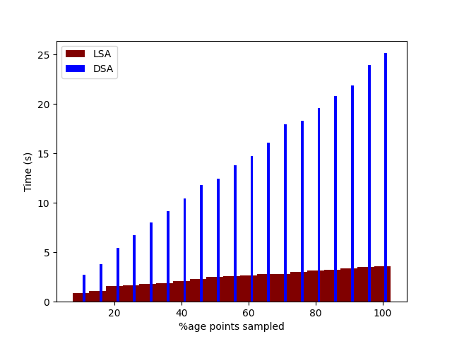
Figure 3: Prediction times on the MacBook with different sampling sizes. DSA was run without batch multithreading.

	LSA			DSA
	orig.	impr.		orig.	impr. (ST)	impr. (MT)
MacBook Pro	0:10	0:04		4:44	0:24	0:13
Desktop-PC	0:12	0:12		2:12	0:25	0:04

TABLE II: Runtime comparison in mm:ss of our improved (impr.) and the original (orig.) SA implementation. (ST/MT = Single/Multi-threaded batch processing)

VI-B3 RQ₂ (Detection Capability of Refined Approaches)

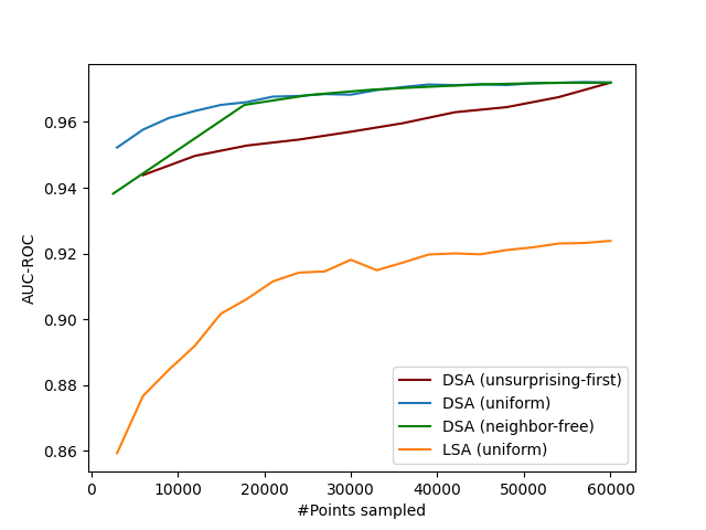
(a) Adversarial Outliers

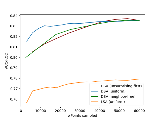
(b) Corrupted Outliers

Figure 4: Out-of-distribution detection performance with varying sample sizes and sampling strategies

To plot the OODD capability at increasing sample size we applied the following procedure: We chose uniformly distributed steps of $s$ for distribution-preserving and unsurprising-first sampling. For $\epsilon$-neighbor-free sampling, we estimated the steps of $\epsilon$ leading to an approximately uniform distribution of $s$ based on sampled distances from the training set. At every step we then averaged, over all 100 re-trained models, the AUC-ROCs. The resulting plots are shown in Figure 4 (adversarial outliers) and Figure 4 (corrupted outliers).

DSA

Using a sample ratio of $\frac{1}{3}$, the capability to detect adversarial samples does not notably decrease (less than 1%) when using either uniform or $\epsilon$-neighbor-free sampling. For unsurprising-first sampling, the decrease is slightly larger, but still less than 2%. While all sampling strategies perform well in detecting corrupted inputs, uniform sampling performs slightly better then the other two strategies – which is notable since this is also the simplest and fastest sampling strategy.

LSA

The OODD performance of LSA appears slightly more impacted by sampling than DSA, in particular on the adversarial outliers. Nonetheless, we still observe good AUC-ROCs at a sampling rate of $\frac{1}{2}$, thus motivating the use of sampling when the training set becomes too big also with LSA.

VI-B4 RQ₃ (Training Instability)

We used the 100 independently but equivalently, trained models to measure the impact of non-determinism on SA’s OODD capability and denote such sensitivity as Training Instability. We measure the training instability using the standard deviation (std) of the AUC-ROC values, as well as their range, i.e., the difference between the highest and the lowest observed AUC-ROC. Our results are shown in table Table I. We observe that training instability, in particular for LSA, is high enough to be possibly relevant in practical use-cases.

KDE, and thus LSA depend on one important hyperparameter: the bandwidth used when fitting KDE. To see whether we can use this hyperparameter to reduce training instability, we ran LSA to perform OODD using the adversarial datasets under a selection of different bandwidths. The resulting AUC-ROC distributions for various bandwidths are shown in Figure 5. They confirm that indeed, bandwidth selection has a high impact on the distribution of AUC-ROCs, as apparent from the variability of the inter-quartile range across bandwidths. Heuristics such as Scott’s Rule (default in LSA) or Silverman’s Rule provide good results, ensuring low instability in our case study.

VI-C Threats to Validity

The primary threat to validity of our study is the low number of test subjects: While we considered two structurally different types of outliers, we use only one underlying dataset: MNIST. Furthermore, we acknowledge that MNIST is a comparably small and clean dataset, which may further hinder generalizability of our results for real world, large and noisy datasets. Note however that this threat does not apply to all our results: First, the fact that sampling-based DSA is much faster is due to analytical properties of sampling that generalize to other datasets. Furthermore, to raise the issue that LSA can be sensitive to random influences during training, one example showing such sensitivity is sufficient.

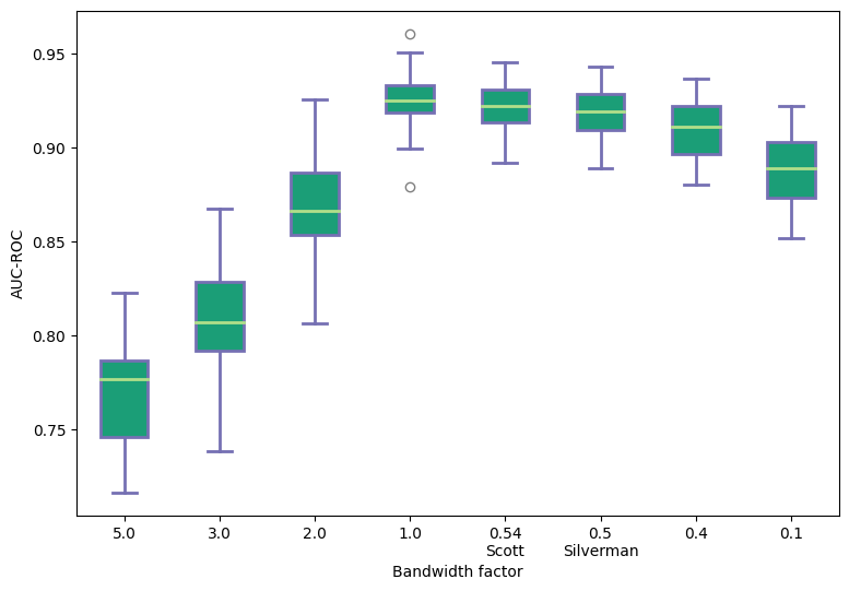
Figure 5: Distribution of OODD AUC-ROC using the adversarial outliers for selected KDE bandwidths

VII Future Work

Reproduction of our experiments on different datasets, different models, and different layers used for AT collections are required to generalize our findings on the OODD capability of sampling based DSA and to support the choice of sampling method. In particular, future studies should consider datasets which are currently harder to be used for OODD, such as noisy and heavily unbalanced datasets. Furthermore, our SA refinements should be compared to existing refinements of SA, in particular Mahalanobis based SA[20].

More experiments on other datasets are required to further enlighten the training instability of SA and to confirm or reject the hypothesis that LSA is typically more sensitive to random influences during training than DSA.

VIII Conclusion

A major weakness of SA is that SA calculation does not scale well with large training datasets. We mitigate this weakness by providing both a faster implementation of plain SA and by suggesting a performance improvement of SA through training set sampling. In our benchmark experiments, our plain DSA implementation was up to 33 times faster than the implementation of DSA released upon its first publication. On MNIST, our sampling strategies further halved the runtime, at a very small cost in terms of reduced OODD AUC-ROC (1%). Our experiments also raise the concern of training instability in SA, i.e., a high sensitivity of its performance to random influences during training.

IX Data Availability

We release the reproduction package of our paper under a permissive MIT license.

References

- [1] J. Kim, R. Feldt, and S. Yoo, “Guiding deep learning system testing using surprise adequacy,” in 2019 IEEE/ACM 41st International Conference on Software Engineering (ICSE). IEEE, 2019, pp. 1039–1049.
- [2] A. Stocco, M. Weiss, M. Calzana, and P. Tonella, “Misbehaviour prediction for autonomous driving systems,” in Proceedings of 42nd International Conference on Software Engineering. ACM, 2020, p. 12 pages.
- [3] D. Hendrycks, M. Mazeika, and T. Dietterich, “Deep anomaly detection with outlier exposure,” in International Conference on Learning Representations, 2018.
- [4] J. Kim, R. Feldt, and S. Yoo. (2018) Source code: Guiding deep learning system testing using surprise adequacy. [Online]. Available: https://github.com/coinse/sadl
- [5] V. C. Raykar, R. Duraiswami, and L. H. Zhao, “Fast computation of kernel estimators,” Journal of Computational and Graphical Statistics, vol. 19, no. 1, pp. 205–220, 2010.
- [6] Y. Feng, Q. Shi, X. Gao, J. Wan, C. Fang, and Z. Chen, “Deepgini: prioritizing massive tests to enhance the robustness of deep neural networks,” in Proceedings of the 29th ACM SIGSOFT International Symposium on Software Testing and Analysis, 2020, pp. 177–188.
- [7] S. Gerasimou, H. F. Eniser, A. Sen, and A. Cakan, “Importance-driven deep learning system testing,” arXiv preprint arXiv:2002.03433, 2020.
- [8] W. Shen, Y. Li, L. Chen, Y. Han, Y. Zhou, and B. Xu, “Multiple-boundary clustering and prioritization to promote neural network retraining,” in 2020 35th IEEE/ACM International Conference on Automated Software Engineering (ASE), 2020, pp. 410–422.
- [9] H. F. Eniser, M. Christakis, and V. Wüstholz, “Raid: Randomized adversarial-input detection for neural networks,” arXiv preprint arXiv:2002.02776, 2020.
- [10] Y. Wang, Z. Li, J. Xu, P. Yu, and X. Ma, “Fast robustness prediction for deep neural network,” in Proceedings of the 11th Asia-Pacific Symposium on Internetware, 2019, pp. 1–10.
- [11] Y.-H. Wang, Z.-N. Li, J.-W. Xu, P. Yu, T. Chen, and X.-X. Ma, “Predicted robustness as qos for deep neural network models,” Journal of Computer Science and Technology, vol. 35, no. 5, pp. 999–1015, 2020.
- [12] T. Byun, V. Sharma, A. Vijayakumar, S. Rayadurgam, and D. Cofer, “Input prioritization for testing neural networks,” in 2019 IEEE International Conference On Artificial Intelligence Testing (AITest), 2019, pp. 63–70.
- [13] G. Jahangirova and P. Tonella, “An empirical evaluation of mutation operators for deep learning systems,” in 2020 IEEE 13th International Conference on Software Testing, Validation and Verification (ICST), 2020, pp. 74–84.
- [14] Y. Dong, P. Zhang, J. Wang, S. Liu, J. Sun, J. Hao, X. Wang, L. Wang, J. S. Dong, and D. Ting, “There is limited correlation between coverage and robustness for deep neural networks,” arXiv preprint arXiv:1911.05904, 2019.
- [15] S. Yan, G. Tao, X. Liu, J. Zhai, S. Ma, L. Xu, and X. Zhang, “Correlations between deep neural network model coverage criteria and model quality,” in Proceedings of the 28th ACM Joint European Software Engineering Conference and Symposium on the Foundations of Software Engineering (ESEC/FSE), 2020.
- [16] J. Chen, M. Yan, Z. Wang, Y. Kang, and Z. Wu, “Deep neural network test coverage: How far are we?” arXiv preprint arXiv:2010.04946, 2020.
- [17] Z. Li, X. Ma, C. Xu, J. Xu, C. Cao, and J. Lü, Operational Calibration: Debugging Confidence Errors for DNNs in the Field. New York, NY, USA: Association for Computing Machinery, 2020.
- [18] S. Kim and S. Yoo, “Evaluating surprise adequacy for question answering,” in Proceedings of the IEEE/ACM 42nd International Conference on Software Engineering Workshops, 2020, pp. 197–202.
- [19] W. Ma, M. Papadakis, A. Tsakmalis, M. Cordy, and Y. L. Traon, “Test selection for deep learning systems,” arXiv preprint arXiv:1904.13195, 2019.
- [20] J. Kim, J. Ju, R. Feldt, and S. Yoo, “Reducing dnn labelling cost using surprise adequacy: An industrial case study for autonomous driving,” arXiv preprint arXiv:2006.00894, 2020.
- [21] Y. LeCun, L. Bottou, Y. Bengio, and P. Haffner, “Gradient-based learning applied to document recognition,” Proceedings of the IEEE, vol. 86, no. 11, pp. 2278–2324, 1998.
- [22] V. Riccio, G. Jahangirova, A. Stocco, N. Humbatova, M. Weiss, and P. Tonella, “Testing machine learning based systems: a systematic mapping,” Empirical Software Engineering, vol. 25, no. 6, pp. 5193–5254, 2020.
- [23] J. Rauber, W. Brendel, and M. Bethge, “Foolbox: A python toolbox to benchmark the robustness of machine learning models,” in Reliable Machine Learning in the Wild Workshop, 34th International Conference on Machine Learning, 2017.
- [24] N. Mu and J. Gilmer, “Mnist-c: A robustness benchmark for computer vision,” arXiv, 2019.
- [25] M. Weiss and P. Tonella, “Fail-safe execution of deep learning based systems through uncertainty monitoring,” arXiv, 2021.