Resonance driving terms and tune spread with amplitude driven a beam-beam long range kick and a DC wire kick

Abstract

This document presents in detail the derivation of the formulas that describe the resonance driving terms and the tune spread with amplitude generated by the beam-beam long range interactions and the DC wire compensators in cyclical machines. This analysis make use of the weak-strong approximation.

1 Introduction

This document presents in detail the derivation of the formulas that describe the resonance driving terms (RDT) and the tune spread with amplitude (TSA) generated by the beam-beam long range (BBLR) interactions and the DC wire compensators in cyclical machines. For the study of the long range beam-beam interactions, the weak-strong approximation [1, 5] is used. According to this, the particles in the “weak” beam interact with the electromagnetic field generated by the charge distribution of the “strong” beam while the latter beam is not affected by the charge distribution of the former one. For the calculation of the resonance driving terms (RDT), the treatment presented in [4, 2] is followed while for the calculation of the tune spread with amplitude (TSA), the first order perturbation theory [3] is used.

2 BBLR and CD wire compensator effective electric and magnetic fields

The charge distributions that generate the BBLR kicks is described by a two dimensional Gaussian at the transverse plane and at the longitudinal one by a line distribution since $\sigma_{s}>>\sigma_{\chi}$ with $\chi=x,y$. From such a charge distribution, the resultant transverse electromagnetic field satisfies the formula $B_{\phi}=-\beta_{ls}E_{r}/c$ in the lab rest frame. Therefore, the integrated Lorentz force experienced by a test particle in the weak beam with negligible transverse velocity is given by:

$$\int\vec{F}_{we}~{}ds= \int q(\vec{E}+\vec{u}_{we}\times\vec{B})~{}ds\Rightarrow$$

$$\int F_{we}~{}ds= q(1+\beta_{we}\beta_{ls})~{}\delta_{D}(s-s_{0}+u_{we}t)\int E_{r}~{}ds$$

$$= q(1+\beta_{we}\beta_{ls})~{}\frac{\delta_{D}(s-s_{0})}{2}\int E_{r}~{}ds$$

$$= q(\mathcal{E}_{x}+\mathcal{E}_{y}).$$ (1)

$q$ is the electric charge of the test particle, $\delta_{D}$ is the Dirac delta function, $s=s_{0}+u_{we}t$, $\delta_{D}(2x)\equiv\delta_{D}(x)/2$, $\beta_{ls}=-u_{st}/c$, $\beta_{we}=u_{we}/c$ and $c$ is the speed of light. The velocities $u_{st}$ and $u_{we}$ are measured in the lab rest frame and are the ones of the strong and weak bunches, respectively. A detailed derivation of the electromagnetic field that describe the beam-beam interactions is presented in [1, 5]. Using these results the expressions for the effective electric ($\mathcal{E}_{\chi}$) and effective magnetic ($\mathcal{B}_{\chi}$) fields that describe the BBLR interactions for round ($\sigma_{\chi}=\sigma_{\psi}=\sigma$) and elliptical bunches ($\sigma_{\chi}>\sigma_{\psi}$) are given by:

$$\mathcal{B}_{x}=\frac{\beta_{ls}}{c}\mathcal{E}_{y}$$ (2a)

$$\mathcal{B}_{y}=-\frac{\beta_{ls}}{c}\mathcal{E}_{x}$$ (2b)

$$\mathcal{E}=\mathcal{E}_{\psi}+\mathrm{i}\mathcal{E}_{\chi}=\mathcal{L}f\delta_{D}(s-s_{0})$$ (2c)

$$\mathcal{L}=\begin{cases}\frac{N_{p}q(1+\beta_{we}\beta_{ls})}{4\epsilon_{0}\pi}&\ \ \ \text{for }\sigma_{\chi}=\sigma_{\psi}=\sigma\\ \frac{N_{p}q(1+\beta_{we}\beta_{ls})}{4\epsilon_{0}\sqrt{\pi}\varDelta_{\chi}}&\ \ \ \text{for }\sigma_{\chi}>\sigma_{\psi}.\end{cases}$$ (2d)

$$f=\begin{cases}\frac{\psi+\widetilde{\psi}+\mathrm{i}(\chi+\widetilde{\chi})}{(\chi+\widetilde{\chi})^{2}+(\psi+\widetilde{\psi})^{2}}\left(1-\mathtt{Exp}\left[-\frac{(\chi+\widetilde{\chi})^{2}+(\psi+\widetilde{\psi})^{2}}{2\sigma^{2}}\right]\right)&\ \ \ \text{for }\sigma_{\chi}=\sigma_{\psi}=\sigma\\ \mathtt{Exp}\left[-\left(\frac{\chi+\widetilde{\chi}+\mathrm{i}(\psi+\widetilde{\psi})}{\varDelta_{\chi}}\right)^{2}\right]\times\\ \left(\mathtt{Erf}\left[\frac{(\psi+\widetilde{\psi})\sigma_{\chi}^{2}-\mathrm{i}(\chi+\widetilde{\chi})\sigma_{\psi}^{2}}{\sigma_{\chi}\sigma_{\psi}\varDelta_{\chi}}\right]+\mathtt{Erf}\left[\frac{\mathrm{i}(\chi+\widetilde{\chi})-(\psi+\widetilde{\psi})}{\varDelta_{\chi}}\right]\right)&\ \ \ \text{for }\sigma_{\chi}>\sigma_{\psi}.\end{cases}$$ (2e)

For round bunches $(\sigma_{\chi}=\sigma_{\psi}=\sigma)$ $\chi=x$ and $\psi=y$ while for elliptical ones $(\sigma_{\chi}>\sigma_{\psi})$ $\chi=x,y$ and $\psi=x$ if $\chi=y$ or $\psi=y$ if $\chi=x$. The symbols $(\widetilde{\chi},\widetilde{\psi})$ represent the transverse position of the weak bunch measured from the center of the strong bunch, where $(\chi,\psi)$ is the transverse position of the test particle measured from the center of the weak bunch, $\epsilon_{0}$ is the vacuum permittivity, $\varDelta_{\chi}=\sqrt{2\left(\sigma_{\chi}^{2}-\sigma_{\psi}^{2}\right)}$ and $\mathtt{Erf}\left[\Xi\right]$ is the error function with $\Xi$ a complex number.

The magnetic field ($B_{w}$) generated by a wire compensator of length $L_{w}$ can be calculated with the use of the Biot-Savart law [6]. However, since the wire length (a few meters long) is quite larger than the distance of the weak beam from the wire (less than a few centimeters), the magnetic field of an infinite long wire can be used. Thus, the integrated-effective magnetic field $\mathcal{B}_{w}$ in complex form is written as:

$$\mathcal{B}_{w}=\mathcal{B}_{wy}+\mathrm{i}\mathcal{B}_{wx}=\mathcal{L}_{w}f_{w}\delta_{D}(s-s_{0}),$$ (3a)

$$\mathcal{L}_{w}=\frac{\mu_{0}I_{w}}{2\pi},$$ (3b)

$$f_{w}=\frac{1}{\mathcal{Z}_{r}+\mathcal{Z}_{wb}}=\sum_{u=0}^{\infty}f_{w}^{(u)}=\sum_{u=0}^{\infty}\frac{(-1)^{u}}{\mathcal{Z}_{wb}^{u+1}}\mathcal{Z}_{r}^{u}=\sum_{u=0}^{\infty}c_{u}\mathcal{Z}_{r}^{u},$$ (3c)

where $I_{w}=\mathcal{J}_{w}L_{w}$ is the integrated current, $\mathcal{J}_{w}$ is the wire current, the $\mathcal{Z}_{r}=x+\mathrm{i}y$ is the test particle position measured from the weak beam and $\mathcal{Z}_{wb}=x_{wb}+\mathrm{i}y_{wb}$ is the position of the weak beam measured from the wire. Since $\mathcal{Z}_{wb}$ must be quite larger that the $\mathcal{Z}_{r}$, the function $f_{w}$ can be also expressed in a multipolar series as shown in Eq. (3c) with multipole strength $c_{u}=\frac{(-1)^{u}}{\mathcal{Z}_{wb}^{u+1}}$.

The effective magnetic field generated by a bunch in the strong beam ($\mathcal{B}$) and the one generated by a wire compensator ($\mathcal{B}_{w}$) are quite similar away from their sources. This can be seen in Figs. 1 where the magnetic fields at distances larger than $2~{}\sigma$ from their sources $\Big{(}\sqrt{(\chi+\widetilde{\chi})^{2}+(\psi+\widetilde{\psi})^{2}}\geq 2~{}\sigma$ and $\sqrt{\mathtt{Re}\left[\mathcal{Z}_{r}+\mathcal{Z}_{wb}\right]^{2}+\mathtt{Im}\left[\mathcal{Z}_{r}+\mathcal{Z}_{wb}\right]^{2}}\geq 2~{}\sigma\Big{)}$ are plotted. The $\mathcal{B}_{wx}$ and $\mathcal{B}_{wy}$ are shown in Fiq. 1a while the $\mathcal{B}_{x}$ and $\mathcal{B}_{y}$ for a charge distribution with $\sigma_{x}>\sigma_{y}$ can be seen in Fig. 1b.

Any magnetic field with only transverse components can be derived from a vector potential $A=A_{s}(x,y)$ using the equations $\vec{B}=\nabla\times\vec{A}$ and $\nabla\cdot\vec{A}=0$. Based on this, the Eqs. (2e and 3) can be obtained from an effective vector potential $\mathcal{A}_{s}=\mathcal{A}_{s}(x,y)$ according to the formulas $\mathcal{B}_{x}=\frac{d\mathcal{A}_{s}}{dy}$ and $\mathcal{B}_{y}=-\frac{d\mathcal{A}_{s}}{dx}$. Therefore, the Hamiltonian that describes the BBLR and wire kicks is of the form $H=-\frac{q}{P_{0}}\mathcal{A}_{s}$ and the solution of Hamilton equations are written as:

$$\frac{dx}{ds}=0\Rightarrow x=x^{i}$$ (4a)

$$\frac{dp_{x}}{ds}=-\frac{q}{P_{0}}\mathcal{B}_{y}\Rightarrow p_{x}=p_{x}^{i}-\frac{q}{P_{0}}\mathcal{B}_{y}(x^{i},y^{i};s_{0})$$ (4b)

$$\frac{dy}{ds}=0\Rightarrow y=y^{i}$$ (4c)

$$\frac{dp_{y}}{ds}=\frac{q}{P_{0}}\mathcal{B}_{x}\Rightarrow p_{y}=p_{y}^{i}+\frac{q}{P_{0}}\mathcal{B}_{x}(x^{i},y^{i};s_{0})$$ (4d)

$$\frac{dl}{ds}=0\Rightarrow l=l^{i}$$ (4e)

$$\frac{d\delta}{ds}=0\Rightarrow\delta=\delta^{i}$$ (4f)

where the effective fields are calculated at $s_{0}$ and the subscript $i$ denote the initial values. In a circular accelerator like the HL-LHC, the particles of the weak beam experience the BBLR and wire kicks (described in Eqs. (4)) at each revolution at specific positions. In other words, each of these kicks is periodic with a period equal to the revolution frequency and for that reason different resonances can be excited. The strength of the resonances (RDT_χ) driven by the different types of the BBLR kicks ($\sigma_{x}>\sigma_{y}$, $\sigma_{y}>\sigma_{x}$ and $\sigma_{x}=\sigma_{y}=\sigma$) and from the wire kick are calculated in the following sections.

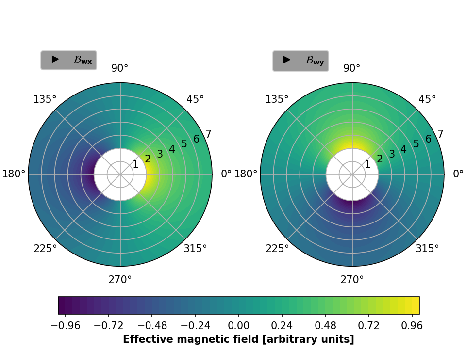
(a)

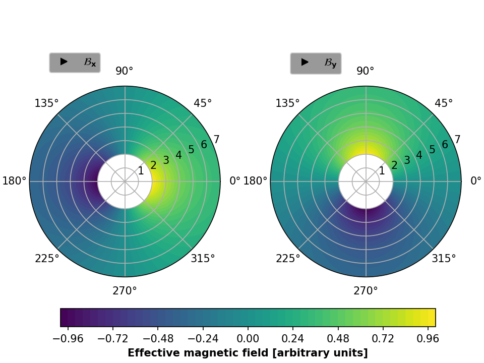
(b)

Figure 1: Transverse effective magnetic field from: a) a wire compensator and b) a charge distribution with $\sigma_{x}>\sigma_{y}$.

3 Resonance driving terms

Using the Eqs. (2e 3, 4b and 4d) the strength of the resonances (RDT_χ) exited by the BBLR and wire kicks is calculated. In the following calculations the contribution from a non zero $\delta$ and the desertion (coupling of the transverse motion with the longitudinal one) is not explicitly expressed. However, in order to extract this information the action $J_{\chi}$ can be replaced by $\frac{\left(\sqrt{\frac{2\beta_{\chi}J_{\chi}}{\widetilde{\delta}}}+\frac{D_{\chi}\delta+\mathcal{O}_{\chi_{p}}\left(\delta^{2}\right)}{\mathtt{Cos}\left[\phi_{\chi}\right]}\right)^{2}}{2\beta_{\chi}}$ with $\chi=x,y$.

3.1 RDT_χ driven by elliptical bunches with $\sigma_{x}>\sigma_{y}$

For elliptical strong bunches with $\sigma_{x}>\sigma_{y}$, the transverse momentum deviation is defined by the following expressions:

$$\frac{dp_{x}}{ds}=\frac{q}{P_{0}}\frac{\beta_{ls}}{c}\mathcal{L}_{x}Im[f_{x}]\delta_{D}(s-s_{0})$$ (5a)

$$\frac{dp_{y}}{ds}=\frac{q}{P_{0}}\frac{\beta_{ls}}{c}\mathcal{L}_{x}Re[f_{x}]\delta_{D}(s-s_{0})$$ (5b)

where the $\mathcal{L}_{x}$ and $f_{x}$ are equal to $\mathcal{L}$ and $f$ (Eqs. (2e and 2d)) when $\sigma_{x}>\sigma_{y}$. The function $f_{x}$ after a Taylor series expansions around the complex numbers $z=x+\mathrm{i}y$, $z_{1}=y\sigma_{x}^{2}-\mathrm{i}x\sigma_{y}^{2}$ and $z_{2}=\mathrm{i}x-y$ is written as:

$$f_{x}=\sum_{u=0}^{\infty}c_{u}(x+\mathrm{i}y)^{u}\left(\sum_{n=0}^{\infty}g_{n}\left(\frac{y\sigma_{x}^{2}-\mathrm{i}x\sigma_{y}^{2}}{\sigma_{x}\sigma_{y}\varDelta_{x}}\right)^{n}+\sum_{m=0}^{\infty}w_{m}\left(\frac{\mathrm{i}x-y}{\varDelta_{x}}\right)^{m}\right)$$ (6)

Each of the coefficients $c_{u}$, $g_{n}$ and $w_{m}$ form a holonomic sequence and are given by the following recursive relations:

$$c_{0}=\mathtt{Exp}\left[-\left(\frac{\widetilde{x}+\mathrm{i}\widetilde{y}}{\varDelta_{x}}\right)^{2}\right]$$ (7a)

$$c_{1}=-\frac{2c_{0}}{\varDelta_{x}^{2}}(\widetilde{x}+\mathrm{i}\widetilde{y})$$ (7b)

$$c_{u}=\frac{-2c_{u-2}-2(\widetilde{x}+\mathrm{i}\widetilde{y})c_{u-1}}{u\varDelta_{x}^{2}}~{}~{}\text{for}~{}u=2,3,...$$ (7c)

$$g_{0}=\mathtt{Erf}\left[\frac{\widetilde{y}\sigma_{x}^{2}-\mathrm{i}\widetilde{x}\sigma_{y}^{2}}{\sigma_{x}\sigma_{y}\varDelta_{x}}\right]$$ (7d)

$$g_{1}=\frac{2}{\sqrt{\pi}}\mathtt{Exp}\left[-\left(\frac{\widetilde{y}\sigma_{x}^{2}-\mathrm{i}\widetilde{x}\sigma_{y}^{2}}{\sigma_{x}\sigma_{y}\varDelta_{x}}\right)^{2}\right]$$ (7e)

$$g_{n}=\frac{-2\sigma_{x}\sigma_{y}\varDelta_{x}(n-2)g_{n-2}-2(\widetilde{y}\sigma_{x}^{2}-\mathrm{i}\widetilde{x}\sigma_{y}^{2})(n-1)g_{n-1}}{n(n-1)\sigma_{x}\sigma_{y}\varDelta_{x}}~{}~{}\text{for}~{}n=2,3,...$$ (7f)

$$w_{0}=\mathtt{Erf}\left[\frac{\mathrm{i}\widetilde{x}-\widetilde{y}}{\varDelta_{x}}\right]$$ (7g)

$$w_{1}=\frac{2}{\sqrt{\pi}}\mathtt{Exp}\left[-\left(\frac{\mathrm{i}\widetilde{x}-\widetilde{y}}{\varDelta_{x}}\right)^{2}\right]$$ (7h)

$$w_{m}=\frac{-2\varDelta_{x}(m-2)w_{m-2}-2(\mathrm{i}\widetilde{x}-\widetilde{y})(m-1)w_{m-1}}{m(m-1)\varDelta_{x}}~{}~{}\text{for}~{}m=2,3,....$$ (7i)

Moving from the coordinates ($x,y$) to the action angle variables ($J_{x},\phi_{x},J_{y},\phi_{y}$) according to the transformations $x=\sqrt{2\beta_{x}J_{x}}\mathtt{Cos}\left[\phi_{x}\right]$ and $y=\sqrt{2\beta_{y}J_{y}}\mathtt{Cos}\left[\phi_{y}\right]$, the $f_{x}$ is defined by:

$$f_{x}=\sum_{u=0}^{\infty}\sum_{n=0}^{\infty}\sum_{m=0}^{\infty}f_{x}^{(u,n,m)}$$ (8a)

$$\begin{split}f_{x}^{(u,n,m)}=&\frac{c_{u}g_{n}}{(\sigma_{x}\sigma_{y}\varDelta_{x})^{n}}\sum_{l_{0}=0}^{u}\sum_{l_{1}=0}^{n}\binom{u}{l_{0}}\binom{n}{l_{1}}\left(\sqrt{2\beta_{x}J_{x}}\right)^{l_{0}}\left(-\mathrm{i}\sigma_{y}^{2}\sqrt{2\beta_{x}J_{x}}\right)^{l_{1}}\left(\mathrm{i}\sqrt{2\beta_{y}J_{y}}\right)^{u-l_{0}}~{}\times\\ &\left(\sigma_{x}^{2}\sqrt{2\beta_{y}J_{y}}\right)^{n-l_{1}}\left(\mathtt{Cos}\left[\phi_{x}\right]\right)^{l_{0}+l_{1}}\left(\mathtt{Cos}\left[\phi_{y}\right]\right)^{u+n-(l_{0}+l_{1})}~{}+\\ &\frac{c_{u}w_{m}}{\varDelta_{x}^{m}}\sum_{l_{0}=0}^{u}\sum_{l_{2}=0}^{m}\binom{u}{l_{0}}\binom{m}{l_{2}}\left(\sqrt{2\beta_{x}J_{x}}\right)^{l_{0}}\left(\mathrm{i}\sqrt{2\beta_{x}J_{x}}\right)^{l_{2}}\left(\mathrm{i}\sqrt{2\beta_{y}J_{y}}\right)^{u-l_{0}}~{}\times\\ &\left(-\sqrt{2\beta_{y}J_{y}}\right)^{m-l_{2}}\left(\mathtt{Cos}\left[\phi_{x}\right]\right)^{l_{0}+l_{2}}\left(\mathtt{Cos}\left[\phi_{y}\right]\right)^{u+m-(l_{0}+l_{2})}.\end{split}$$ (8b)

Since the $f_{x}$ and so the $f_{x}^{(u,n,m)}$ are periodic with period of one revolution (the different BBLR kicks are applied at every revolution at specific positions) it is more convenient to use a new set of canonical variables where the new angle $\mu$ will be change linearly with $s$ for the linear motion. Using a generating function of the second type [3] the transformation to the new canonical conjugate variables is given by the following equations:

$$\mathcal{F}_{2}(\phi_{x},\widehat{J}_{x},\phi_{y},\widehat{J}_{y},s)=\widehat{J}_{x}\left(\phi_{x}+\frac{2\pi Q_{x}s}{\mathcal{C}}-\int_{0}^{s}\frac{ds^{\prime}}{\beta_{x}(s^{\prime})}\right)+\widehat{J}_{y}\left(\phi_{y}+\frac{2\pi Q_{y}s}{\mathcal{C}}-\int_{0}^{s}\frac{ds^{\prime}}{\beta_{y}(s^{\prime})}\right)$$ (9a)

$$J_{x}=\frac{\partial\mathcal{F}_{2}}{\partial\phi_{x}}=\widehat{J}_{x}$$ (9b)

$$\mu_{x}=\frac{\partial\mathcal{F}_{2}}{\partial\widehat{J}_{x}}=\phi_{x}+\frac{2\pi Q_{x}s}{\mathcal{C}}-\int_{0}^{s}\frac{ds^{\prime}}{\beta_{x}(s^{\prime})}=\phi_{x}+\psi_{x}(s)$$ (9c)

$$J_{y}=\frac{\partial\mathcal{F}_{2}}{\partial\phi_{y}}=\widehat{J}_{y}$$ (9d)

$$\mu_{y}=\frac{\partial\mathcal{F}_{2}}{\partial\widehat{J}_{y}}=\phi_{y}+\frac{2\pi Q_{y}s}{\mathcal{C}}-\int_{0}^{s}\frac{ds^{\prime}}{\beta_{y}(s^{\prime})}=\phi_{y}+\psi_{y}(s).$$ (9e)

The $Q_{x}$ and $Q_{y}$ are the working tunes, $\beta_{x}$ and $\beta_{y}$ are the optical betatronic functions, $\mathcal{C}$ is the lattice circumference and $\psi_{\chi}(s)=\frac{2\pi Q_{\chi}s}{\mathcal{C}}-\int_{0}^{s}\frac{ds^{\prime}}{\beta_{\chi}(s^{\prime})}$ with $\chi=x,y$. Using the above transformation and rewriting the cosines in complex form the $f_{x}^{(u,n,m)}$ is written as:

$$\begin{split}f_{x}^{(u,n,m)}=&\sum_{l_{0}=0}^{u}\sum_{l_{1}=0}^{n}\sum_{\kappa_{1}=0}^{\zeta_{1}}\sum_{\tau_{1}=0}^{\xi_{1}}J_{x}^{\zeta_{1}/2}~{}J_{y}^{\xi_{1}/2}~{}h_{l_{0},l_{1},\kappa_{1},\tau_{1}}^{(u,n)}\mathtt{Exp}\left[\mathrm{i}\left(\mu_{x}(2\kappa_{1}-\zeta_{1})+\mu_{y}(2\tau_{1}-\xi_{1})\right)\right]~{}+\\ &\sum_{l_{0}=0}^{u}\sum_{l_{2}=0}^{m}\sum_{\kappa_{2}=0}^{\zeta_{2}}\sum_{\tau_{2}=0}^{\xi_{2}}J_{x}^{\zeta_{2}/2}~{}J_{y}^{\xi_{2}/2}~{}h_{l_{0},l_{2},\kappa_{2},\tau_{2}}^{(u,m)}\mathtt{Exp}\left[\mathrm{i}\left(\mu_{x}(2\kappa_{2}-\zeta_{2})+\mu_{y}(2\tau_{2}-\xi_{2})\right)\right]\end{split}$$ (10a)

$$\begin{split}h_{l_{0},l_{1},\kappa_{1},\tau_{1}}^{(u,n)}=&\frac{c_{u}g_{n}}{(\sigma_{x}\sigma_{y}\varDelta_{x})^{n}}\frac{1}{2^{\zeta_{1}+\xi_{1}}}\binom{u}{l_{0}}\binom{n}{l_{1}}\binom{\zeta_{1}}{\kappa_{1}}\binom{\xi_{1}}{\tau_{1}}\left(\sqrt{2\beta_{x}}\right)^{l_{0}}\left(-\mathrm{i}\sigma_{y}^{2}\sqrt{2\beta_{x}}\right)^{l_{1}}\left(\mathrm{i}\sqrt{2\beta_{y}}\right)^{u-l_{0}}~{}\times\\ &\left(\sigma_{x}^{2}\sqrt{2\beta_{y}}\right)^{n-l_{1}}\mathtt{Exp}\left[-\mathrm{i}\left(\psi_{x}(2\kappa_{1}-\zeta_{1})+\psi_{y}(2\tau_{1}-\xi_{1})\right)\right]\end{split}$$ (10b)

$$\begin{split}h_{l_{0},l_{2},\kappa_{2},\tau_{2}}^{(u,m)}=&\frac{c_{u}w_{m}}{\varDelta_{x}^{m}}\frac{1}{2^{\zeta_{2}+\xi_{2}}}\binom{u}{l_{0}}\binom{m}{l_{2}}\binom{\zeta_{2}}{\kappa_{2}}\binom{\xi_{2}}{\tau_{2}}\left(\sqrt{2\beta_{x}}\right)^{l_{0}}\left(\mathrm{i}\sqrt{2\beta_{x}}\right)^{l_{2}}\left(\mathrm{i}\sqrt{2\beta_{y}}\right)^{u-l_{0}}~{}\times\\ &\left(-\sqrt{2\beta_{y}}\right)^{m-l_{2}}\mathtt{Exp}\left[-\mathrm{i}\left(\psi_{x}(2\kappa_{2}-\zeta_{2})+\psi_{y}(2\tau_{2}-\xi_{2})\right)\right].\end{split}$$ (10c)

with $\zeta_{1}=l_{0}+l_{1}$, $\xi_{1}=u+n-\zeta_{1}$, $\zeta_{2}=l_{0}+l_{2}$, $\xi_{2}=u+m-\zeta_{2}$ and the optical parameters are kept together in the $h_{l_{0},l_{1},\kappa_{1},\tau_{1}}^{(u,n)}$ and $h_{l_{0},l_{2},\kappa_{2},\tau_{2}}^{(u,m)}$ functions. As said, the BBLR kicks affect the beam at every revolution thus, the $f_{x}^{(u,n,m)}$ can be expressed as a Fourier series. The resulted series with its Fourier coefficients $h_{l_{0},l_{1},\kappa_{1},\tau_{1};p1}^{(u,n)}$ and $h_{l_{0},l_{2},\kappa_{2},\tau_{2};p2}^{(u,m)}$ are given by:

$$\begin{split}f_{x}^{(u,n,m)}=&\sum_{l_{0}=0}^{u}\sum_{l_{1}=0}^{n}\sum_{\kappa_{1}=0}^{\zeta_{1}}\sum_{\tau_{1}=0}^{\xi_{1}}\sum_{p_{1}=-\infty}^{\infty}J_{x}^{\zeta_{1}/2}~{}J_{y}^{\xi_{1}/2}~{}h_{l_{0},l_{1},\kappa_{1},\tau_{1};p_{1}}^{(u,n)}~{}\times\\ &\mathtt{Exp}\left[\mathrm{i}\left(\mu_{x}(2\kappa_{1}-\zeta_{1})+\mu_{y}(2\tau_{1}-\xi_{1})-\frac{2\pi~{}s}{\mathcal{C}}p_{1}\right)\right]~{}+\\ &\sum_{l_{0}=0}^{u}\sum_{l_{2}=0}^{m}\sum_{\kappa_{2}=0}^{\zeta_{2}}\sum_{\tau_{2}=0}^{\xi_{2}}\sum_{p_{2}=-\infty}^{\infty}J_{x}^{\zeta_{2}/2}~{}J_{y}^{\xi_{2}/2}~{}h_{l_{0},l_{2},\kappa_{2},\tau_{2};p_{2}}^{(u,m)}~{}\times\\ &\mathtt{Exp}\left[\mathrm{i}\left(\mu_{x}(2\kappa_{2}-\zeta_{2})+\mu_{y}(2\tau_{2}-\xi_{2})-\frac{2\pi~{}s}{\mathcal{C}}p_{2}\right)\right]\end{split}$$ (11a)

$$h_{l_{0},l_{1},\kappa_{1},\tau_{1};p_{1}}^{(u,n)}=\frac{1}{2\pi}\int_{s_{0}}^{s_{0}+\mathcal{C}}h_{l_{0},l_{1},\kappa_{1},\tau_{1}}^{(u,n)}\mathtt{Exp}\left[\mathrm{i}p_{1}~{}\frac{2\pi~{}s}{\mathcal{C}}\right]~{}ds$$ (11b)

$$h_{l_{0},l_{2},\kappa_{2},\tau_{2};p_{2}}^{(u,m)}=\frac{1}{2\pi}\int_{s_{0}}^{s_{0}+\mathcal{C}}h_{l_{0},l_{2},\kappa_{2},\tau_{2}}^{(u,m)}\mathtt{Exp}\left[\mathrm{i}p_{2}~{}\frac{2\pi~{}s}{\mathcal{C}}\right]~{}ds$$ (11c)

The exited resonances are the ones described by the formulas $(2\kappa_{1}-\zeta_{1})Q_{x}+(2\tau_{1}-\xi_{1})Q_{y}=p_{1}$ and $(2\kappa_{2}-\zeta_{2})Q_{x}+(2\tau_{2}-\xi_{2})Q_{y}=p_{2}$ and their strength at $x$ and $y$ plane are defined by:

$$\text{RDT}_{x}=\begin{cases}Im\left[\frac{q}{P_{0}}\frac{\beta_{ls}}{c}\mathcal{L}_{x}~{}h_{l_{0},l_{1},\kappa_{1},\tau_{1};p_{1}}^{(u,n)}\right]~{}~{}\text{for}\ (2\kappa_{1}-\zeta_{1})Q_{x}+(2\tau_{1}-\xi_{1})Q_{y}=p_{1}\\ Im\left[\frac{q}{P_{0}}\frac{\beta_{ls}}{c}\mathcal{L}_{x}~{}h_{l_{0},l_{2},\kappa_{2},\tau_{2};p_{2}}^{(u,m)}\right]~{}~{}\text{for}\ (2\kappa_{2}-\zeta_{2})Q_{x}+(2\tau_{2}-\xi_{2})Q_{y}=p_{2}\end{cases}$$ (12a)

$$\text{RDT}_{y}=\begin{cases}Re\left[\frac{q}{P_{0}}\frac{\beta_{ls}}{c}\mathcal{L}_{x}~{}h_{l_{0},l_{1},\kappa_{1},\tau_{1};p_{1}}^{(u,n)}\right]~{}~{}\text{for}\ (2\kappa_{1}-\zeta_{1})Q_{x}+(2\tau_{1}-\xi_{1})Q_{y}=p_{1}\\ Re\left[\frac{q}{P_{0}}\frac{\beta_{ls}}{c}\mathcal{L}_{x}~{}h_{l_{0},l_{2},\kappa_{2},\tau_{2};p_{2}}^{(u,m)}\right]~{}~{}\text{for}\ (2\kappa_{2}-\zeta_{2})Q_{x}+(2\tau_{2}-\xi_{2})Q_{y}=p_{2}.\end{cases}$$ (12b)

3.2 RDT_χ driven by elliptical bunches with $\sigma_{y}>\sigma_{x}$

For elliptical strong bunches with $\sigma_{y}>\sigma_{x}$ the transverse momentum deviation is defined by the following expressions:

$$\frac{dp_{x}}{ds}=\frac{q}{P_{0}}\frac{\beta_{ls}}{c}\mathcal{L}_{y}Re[f_{y}]\delta(s-s_{0})$$ (13a)

$$\frac{dp_{y}}{ds}=\frac{q}{P_{0}}\frac{\beta_{ls}}{c}\mathcal{L}_{y}Im[f_{y}]\delta(s-s_{0})$$ (13b)

where the $\mathcal{L}_{y}$ and $f_{y}$ are equal to $\mathcal{L}$ and $f$ (Eqs. (2e and 2d)) when $\sigma_{y}>\sigma_{x}$. The $f_{y}$ after a Taylor series expansions and the transformation to action angle variable ($\widehat{J}_{x},\mu_{x},\widehat{J}_{y},\mu_{y}$), is given by the corresponding expressions for the $f_{x}$ (Eqs. (10c)) provided that the alternation between $x$ and $y$ is performed and is written as:

$$\begin{split}f_{y}^{(u,n,m)}=&\sum_{l_{0}=0}^{u}\sum_{l_{1}=0}^{n}\sum_{\kappa_{1}=0}^{\zeta_{1}}\sum_{\tau_{1}=0}^{\xi_{1}}J_{y}^{\zeta_{1}/2}~{}J_{x}^{\xi_{1}/2}~{}h1_{l_{0},l_{1},\kappa_{1},\tau_{1}}^{(u,n)}\mathtt{Exp}\left[\mathrm{i}\left(\mu_{y}(2\kappa_{1}-\zeta_{1})+\mu_{x}(2\tau_{1}-\xi_{1})\right)\right]~{}+\\ &\sum_{l_{0}=0}^{u}\sum_{l_{2}=0}^{m}\sum_{\kappa_{2}=0}^{\zeta_{2}}\sum_{\tau_{2}=0}^{\xi_{2}}J_{y}^{\zeta_{2}/2}~{}J_{x}^{\xi_{2}/2}~{}h1_{l_{0},l_{2},\kappa_{2},\tau_{2}}^{(u,m)}\mathtt{Exp}\left[\mathrm{i}\left(\mu_{y}(2\kappa_{2}-\zeta_{2})+\mu_{x}(2\tau_{2}-\xi_{2})\right)\right]\end{split}$$ (14a)

$$\begin{split}h1_{l_{0},l_{1},\kappa_{1},\tau_{1}}^{(u,n)}=&\frac{c_{u}g_{n}}{(\sigma_{x}\sigma_{y}\varDelta_{y})^{n}}\frac{1}{2^{\zeta_{1}+\xi_{1}}}\binom{u}{l_{0}}\binom{n}{l_{1}}\binom{\zeta_{1}}{\kappa_{1}}\binom{\xi_{1}}{\tau_{1}}\left(\sqrt{2\beta_{y}}\right)^{l_{0}}\left(-\mathrm{i}\sigma_{x}^{2}\sqrt{2\beta_{y}}\right)^{l_{1}}\left(\mathrm{i}\sqrt{2\beta_{x}}\right)^{u-l_{0}}~{}\times\\ &\left(\sigma_{y}^{2}\sqrt{2\beta_{x}}\right)^{n-l_{1}}\mathtt{Exp}\left[-\mathrm{i}\left(\psi_{y}(2\kappa_{1}-\zeta_{1})+\psi_{x}(2\tau_{1}-\xi_{1})\right)\right]\end{split}$$ (14b)

$$\begin{split}h1_{l_{0},l_{2},\kappa_{2},\tau_{2}}^{(u,m)}=&\frac{c_{u}w_{m}}{\varDelta_{y}^{m}}\frac{1}{2^{\zeta_{2}+\xi_{2}}}\binom{u}{l_{0}}\binom{m}{l_{2}}\binom{\zeta_{2}}{\kappa_{2}}\binom{\xi_{2}}{\tau_{2}}\left(\sqrt{2\beta_{y}}\right)^{l_{0}}\left(\mathrm{i}\sqrt{2\beta_{y}}\right)^{l_{2}}\left(\mathrm{i}\sqrt{2\beta_{x}}\right)^{u-l_{0}}~{}\times\\ &\left(-\sqrt{2\beta_{x}}\right)^{m-l_{2}}\mathtt{Exp}\left[-\mathrm{i}\left(\psi_{y}(2\kappa_{2}-\zeta_{2})+\psi_{x}(2\tau_{2}-\xi_{2})\right)\right]\end{split}$$ (14c)

$$c_{0}=\mathtt{Exp}\left[-\left(\frac{\widetilde{y}+\mathrm{i}\widetilde{x}}{\varDelta_{y}}\right)^{2}\right]$$ (14d)

$$c_{1}=-\frac{2~{}c_{0}}{\varDelta_{y}^{2}}(\widetilde{y}+\mathrm{i}\widetilde{x})$$ (14e)

$$\text{for}~{}u=2,3,...~{}~{}c_{u}=\frac{-2c_{u-2}-2(\widetilde{y}+\mathrm{i}\widetilde{x})c_{u-1}}{u~{}\varDelta_{y}^{2}}$$ (14f)

$$g_{0}=\mathtt{Erf}\left[\frac{\widetilde{x}\sigma_{y}^{2}-\mathrm{i}\widetilde{y}\sigma_{x}^{2}}{\sigma_{x}\sigma_{y}\varDelta_{y}}\right]$$ (14g)

$$g_{1}=\frac{2}{\sqrt{\pi}}\mathtt{Exp}\left[-\left(\frac{\widetilde{x}\sigma_{y}^{2}-\mathrm{i}\widetilde{y}\sigma_{x}^{2}}{\sigma_{x}\sigma_{y}\varDelta_{y}}\right)^{2}\right]$$ (14h)

$$\text{for}~{}n=2,3,...~{}~{}g_{n}=\frac{-2\sigma_{x}\sigma_{y}\varDelta_{y}(n-2)q_{n-2}-2(\widetilde{x}\sigma_{y}^{2}-\mathrm{i}\widetilde{y}\sigma_{x}^{2})(n-1)g_{n-1}}{n(n-1)\sigma_{x}\sigma_{y}\varDelta_{y}}$$ (14i)

$$w_{0}=\mathtt{Erf}\left[\frac{\mathrm{i}\widetilde{y}-\widetilde{x}}{\varDelta_{y}}\right]$$ (14j)

$$w_{1}=\frac{2}{\sqrt{\pi}}\mathtt{Exp}\left[-\left(\frac{\mathrm{i}\widetilde{y}-\widetilde{x}}{\varDelta_{y}}\right)^{2}\right]$$ (14k)

$$\text{for}~{}m=2,3,...~{}~{}w_{m}=\frac{-2\varDelta_{y}(m-2)w_{m-2}-2(\mathrm{i}\widetilde{y}-\widetilde{x})(m-1)w_{m-1}}{m(m-1)\varDelta_{y}}.$$ (14l)

The RDT_χ after the Fourier transformation are defined by:

$$\text{RDT}_{x}=\begin{cases}Re\left[\frac{q}{P_{0}}\frac{\beta_{ls}}{c}\mathcal{L}_{y}~{}h1_{l_{0},l_{1},\kappa_{1},\tau_{1};p_{1}}^{(u,n)}\right]~{}~{}\text{for}\ (2\kappa_{1}-\zeta_{1})Q_{y}+(2\tau_{1}-\xi_{1})Q_{x}=p_{1}\\ Re\left[\frac{q}{P_{0}}\frac{\beta_{ls}}{c}\mathcal{L}_{y}~{}h1_{l_{0},l_{2},\kappa_{2},\tau_{2};p_{2}}^{(u,m)}\right]~{}~{}\text{for}\ (2\kappa_{2}-\zeta_{2})Q_{y}+(2\tau_{2}-\xi_{2})Q_{x}=p_{2}\end{cases}$$ (15a)

$$\text{RDT}_{y}=\begin{cases}Im\left[\frac{q}{P_{0}}\frac{\beta_{ls}}{c}\mathcal{L}_{y}~{}h1_{l_{0},l_{1},\kappa_{1},\tau_{1};p_{1}}^{(u,n)}\right]~{}~{}\text{for}\ (2\kappa_{1}-\zeta_{1})Q_{y}+(2\tau_{1}-\xi_{1})Q_{x}=p_{1}\\ Im\left[\frac{q}{P_{0}}\frac{\beta_{ls}}{c}\mathcal{L}_{y}~{}h1_{l_{0},l_{2},\kappa_{2},\tau_{2};p_{2}}^{(u,m)}\right]~{}~{}\text{for}\ (2\kappa_{2}-\zeta_{2})Q_{y}+(2\tau_{2}-\xi_{2})Q_{x}=p_{2}\end{cases}$$ (15b)

$$h1_{l_{0},l_{1},\kappa_{1},\tau_{1};p_{1}}^{(u,n)}=\frac{1}{2\pi}\int_{s_{0}}^{s_{0}+\mathcal{C}}h1_{l_{0},l_{1},\kappa_{1},\tau_{1}}^{(u,n)}\mathtt{Exp}\left[\mathrm{i}p_{1}~{}\frac{2\pi~{}s}{\mathcal{C}}\right]~{}ds$$ (15c)

$$h1_{l_{0},l_{2},\kappa_{2},\tau_{2};p_{2}}^{(u,m)}=\frac{1}{2\pi}\int_{s_{0}}^{s_{0}+\mathcal{C}}h1_{l_{0},l_{2},\kappa_{2},\tau_{2}}^{(u,m)}\mathtt{Exp}\left[\mathrm{i}p_{2}~{}\frac{2\pi~{}s}{\mathcal{C}}\right]~{}ds.$$ (15d)

3.3 RDT_χ driven by round bunches with $\sigma_{x}=\sigma_{y}$

For round strong bunches ($\sigma_{x}=\sigma_{y}=\sigma$) the transverse momentum deflection from a BBLR kick is defined by:

$$\frac{dp_{x}}{ds}=\frac{q}{P_{0}}\frac{\beta_{ls}}{c}\mathcal{L}_{r}f_{r}(x+\widetilde{x})\delta(s-s_{0})$$ (16a)

$$\frac{dp_{y}}{ds}=\frac{q}{P_{0}}\frac{\beta_{ls}}{c}\mathcal{L}_{r}f_{r}(y+\widetilde{y})\delta(s-s_{0})$$ (16b)

$$f_{r}=\frac{1}{R^{2}}\left(1-\mathtt{Exp}\left[-\frac{R^{2}}{2\sigma^{2}}\right]\right)$$ (16c)

where the $\mathcal{L}_{r}$ is equal to $\mathcal{L}$ (Eq. (2d)) when $\sigma_{x}=\sigma_{y}$ and $R^{2}=(x+\widetilde{x})^{2}+(y+\widetilde{y})^{2}$. After a Taylor series expansions the $f_{r}$ is given by the following summation:

$$f_{r}=\sum_{u=0}^{\infty}~{}f_{r}^{(u)}=\sum_{u=0}^{\infty}\frac{(-1)^{u}R^{2u}}{2^{u+1}~{}(u+1)!~{}\sigma^{2(u+1)}}=\sum_{u=0}^{\infty}\frac{(-1)^{u}~{}\left((x+\widetilde{x})^{2}+(y+\widetilde{y})^{2}\right)^{u}}{2^{u+1}~{}(u+1)!~{}\sigma^{2(u+1)}}.$$ (17)

Using the action angle variables $\chi=\sqrt{2\beta_{\chi}J_{\chi}}~{}\mathtt{Cos}\left[\phi_{\chi}\right]$ with $\chi=x,y$ and expanding the binomials, the $f_{r}$ takes the following form:

$$f_{r}=\sum_{u=0}^{\infty}~{}f_{r}^{(u)}$$ (18a)

$$\begin{split}f_{r}^{(u)}=&\sum_{l=0}^{u}\sum_{n=0}^{2l}\sum_{m=0}^{2(u-l)}\frac{(-1)^{u}}{2^{u+1}~{}(u+1)!~{}\sigma^{2(u+1)}}\binom{u}{l}\binom{2l}{n}\binom{2(u-l)}{m}~{}\times\\ &(\sqrt{2\beta_{x}})^{n}~{}\widetilde{x}^{2l-n}~{}(\sqrt{2\beta_{y}})^{m}~{}\widetilde{y}^{2(u-l)-m}~{}\left(\mathtt{Cos}\left[\phi_{x}\right]\right)^{n}~{}\left(\mathtt{Cos}\left[\phi_{y}\right]\right)^{m}.\end{split}$$ (18b)

Rewriting the cosines in complex form ($\mathtt{Cos}\left[\phi_{\chi}\right]=\frac{\mathtt{Exp}[\mathrm{i}\phi_{\chi}]+\mathtt{Exp}[-\mathrm{i}\phi_{\chi}]}{2}$ with $\chi=x,y$) and using the action angle variables ($\widehat{J}_{x},\mu_{x},\widehat{J}_{y},\mu_{y}$) described by the Eqs. (9), the $f_{rx}$ and $f_{ry}$ for a given $u$ are written as:

$$\begin{split}f_{rx}^{(u)}=&(x+\widetilde{x})\sum_{l=0}^{u}f_{r}^{(u)}=\sum_{l=0}^{u}\sum_{n=0}^{2l}\sum_{m=0}^{2(u-l)}\sum_{\tau=0}^{m}J_{x}^{n/2}J_{y}^{m/2}~{}\mathtt{Exp}\left[\mathrm{i}\mu_{y}(2\tau-m)\right]\times\\ &\Bigg{(}\sqrt{J_{x}}~{}\sum_{\kappa=0}^{n+1}~{}h2_{l,n,m,\kappa,\tau}^{(u)}\mathtt{Exp}\left[\mathrm{i}\mu_{x}(2\kappa-n-1)\right]+\sum_{\kappa=0}^{n}~{}h3_{l,n,m,\kappa,\tau}^{(u)}\mathtt{Exp}\left[\mathrm{i}\mu_{x}(2\kappa-n)\right]~{}\Bigg{)}\end{split}$$ (19a)

$$\begin{split}f_{ry}^{(u)}=&(y+\widetilde{y})\sum_{l=0}^{u}f_{r}^{(u)}=\sum_{l=0}^{u}\sum_{n=0}^{2l}\sum_{m=0}^{2(u-l)}\sum_{\kappa=0}^{n}J_{x}^{n/2}J_{y}^{m/2}~{}\mathtt{Exp}\left[\mathrm{i}\mu_{x}(2\kappa-n)\right]\times\\ &\Bigg{(}\sqrt{J_{y}}~{}\sum_{\tau=0}^{m+1}~{}h4_{l,n,m,\kappa,\tau}^{(u)}\mathtt{Exp}\left[\mathrm{i}\mu_{y}(2\tau-m-1)\right]+\sum_{\tau=0}^{m}~{}h5_{l,n,m,\kappa,\tau}^{(u)}\mathtt{Exp}\left[\mathrm{i}\mu_{y}(2\tau-m)\right]~{}\Bigg{)}\end{split}$$ (19b)

$$\begin{split}h2_{l,n,m,\kappa,\tau}^{(u)}=&\frac{(-1)^{u}}{2^{u+n+m+2}~{}(u+1)!~{}\sigma^{2(u+1)}}\binom{u}{l}\binom{2l}{n}\binom{2(u-l)}{m}\binom{n+1}{\kappa}\binom{m}{\tau}\left(\sqrt{2\beta_{x}}\right)^{n+1}~{}\widetilde{x}^{2l-n}~{}\times\\ &\left(\sqrt{2\beta_{y}}\right)^{m}~{}\widetilde{y}^{2(u-l)-m}\mathtt{Exp}\left[-\mathrm{i}\psi_{x}(2\kappa-n-1)\right]\mathtt{Exp}\left[-\mathrm{i}\psi_{y}(2\tau-m)\right]\end{split}$$ (19c)

$$\begin{split}h3_{l,n,m,\kappa,\tau}^{(u)}=&\frac{(-1)^{u}}{2^{u+n+m+1}~{}(u+1)!~{}\sigma^{2(u+1)}}\binom{u}{l}\binom{2l}{n}\binom{2(u-l)}{m}\binom{n}{\kappa}\binom{m}{\tau}\left(\sqrt{2\beta_{x}}\right)^{n}~{}\widetilde{x}^{2l-n+1}~{}\times\\ &\left(\sqrt{2\beta_{y}}\right)^{m}~{}\widetilde{y}^{2(u-l)-m}\mathtt{Exp}\left[-\mathrm{i}\psi_{x}(2\kappa-n)\right]\mathtt{Exp}\left[-\mathrm{i}\psi_{y}(2\tau-m)\right]\end{split}$$ (19d)

$$\begin{split}h4_{l,n,m,\kappa,\tau}^{(u)}=&\frac{(-1)^{u}}{2^{u+n+m+2}~{}(u+1)!~{}\sigma^{2(u+1)}}\binom{u}{l}\binom{2l}{n}\binom{2(u-l)}{m}\binom{n}{\kappa}\binom{m+1}{\tau}\left(\sqrt{2\beta_{x}}\right)^{n}~{}\widetilde{x}^{2l-n}~{}\times\\ &\left(\sqrt{2\beta_{y}}\right)^{m+1}~{}\widetilde{y}^{2(u-l)-m}\mathtt{Exp}\left[-\mathrm{i}\psi_{x}(2\kappa-n)\right]\mathtt{Exp}\left[-\mathrm{i}\psi_{y}(2\tau-m-1)\right]\end{split}$$ (19e)

$$\begin{split}h5_{l,n,m,\kappa,\tau}^{(u)}=&\frac{(-1)^{u}}{2^{u+n+m+1}~{}(u+1)!~{}\sigma^{2(u+1)}}\binom{u}{l}\binom{2l}{n}\binom{2(u-l)}{m}\binom{n}{\kappa}\binom{m}{\tau}\left(\sqrt{2\beta_{x}}\right)^{n}~{}\widetilde{x}^{2l-n}~{}\times\\ &\left(\sqrt{2\beta_{y}}\right)^{m}~{}\widetilde{y}^{2(u-l)-m+1}\mathtt{Exp}\left[-\mathrm{i}\psi_{x}(2\kappa-n)\right]\mathtt{Exp}\left[-\mathrm{i}\psi_{y}(2\tau-m)\right].\end{split}$$ (19f)

Because of the periodic repetition of the BBLR kicks, the $f_{rx}^{(u)}$ and $f_{ry}^{(u)}$ can be written as a Fourier series. This series with their Fourier coefficients $h2_{l,n,m,\kappa,\tau;p_{1}}^{(u)}$, $h3_{l,n,m,\kappa,\tau:p_{2}}^{(u)}$, $h4_{l,n,m,\kappa,\tau;p_{1}}^{(u)}$ and $h5_{l,n,m,\kappa,\tau;p_{2}}^{(u)}$ are given by:

$$\begin{split}f_{rx}^{(u)}=&\sum_{l=0}^{u}\sum_{n=0}^{2l}\sum_{m=0}^{2(u-l)}\sum_{\tau=0}^{m}J_{x}^{n/2}J_{y}^{m/2}~{}\times\\ &\Bigg{(}\sqrt{J_{x}}~{}\sum_{\kappa=0}^{n+1}\sum_{p_{2}=-\infty}^{\infty}~{}h2_{l,n,m,\kappa,\tau;p_{1}}^{(u)}\mathtt{Exp}\left[\mathrm{i}\left(\mu_{x}(2\kappa-n-1)+\mu_{y}(2\tau-m)-\frac{2\pi~{}s}{\mathcal{C}}p_{1}\right)\right]~{}+\\ &\sum_{\kappa=0}^{n}\sum_{p_{1}=-\infty}^{\infty}~{}h3_{l,n,m,\kappa,\tau;p_{2}}^{(u)}\mathtt{Exp}\left[\mathrm{i}\left(\mu_{x}(2\kappa-n)+\mu_{y}(2\tau-m)-\frac{2\pi~{}s}{\mathcal{C}}p_{2}\right)\right]~{}\Bigg{)}\end{split}$$ (20a)

$$\begin{split}f_{ry}^{(u)}=&\sum_{l=0}^{u}\sum_{n=0}^{2l}\sum_{m=0}^{2(u-l)}\sum_{\kappa=0}^{n}J_{x}^{n/2}J_{y}^{m/2}~{}\times\\ &\Bigg{(}\sqrt{J_{y}}~{}\sum_{\tau=0}^{m+1}\sum_{p_{2}=-\infty}^{\infty}~{}h4_{l,n,m,\kappa,\tau;p_{1}}^{(u)}\mathtt{Exp}\left[\mathrm{i}\left(\mu_{x}(2\kappa-n)+\mu_{y}(2\tau-m-1)-\frac{2\pi~{}s}{\mathcal{C}}p_{1}\right)\right]~{}+\\ &\sum_{\tau=0}^{m}\sum_{p_{1}=-\infty}^{\infty}~{}h5_{l,n,m,\kappa,\tau;p_{2}}^{(u)}\mathtt{Exp}\left[\mathrm{i}\left(\mu_{x}(2\kappa-n)+\mu_{y}(2\tau-m)-\frac{2\pi~{}s}{\mathcal{C}}p_{2}\right)\right]~{}\Bigg{)}\end{split}$$ (20b)

$$h2_{l,n,m,\kappa,\tau;p_{1}}^{(u)}=\frac{1}{2\pi}\int_{s_{0}}^{s_{0}+\mathcal{C}}h2_{l,n,m,\kappa,\tau}^{(u)}\mathtt{Exp}\left[\mathrm{i}p_{1}~{}\frac{2\pi~{}s}{\mathcal{C}}\right]~{}ds$$ (20c)

$$h3_{l,n,m,\kappa,\tau;p_{2}}^{(u)}=\frac{1}{2\pi}\int_{s_{0}}^{s_{0}+\mathcal{C}}h3_{l,n,m,\kappa,\tau}^{(u)}\mathtt{Exp}\left[\mathrm{i}p_{2}~{}\frac{2\pi~{}s}{\mathcal{C}}\right]~{}ds$$ (20d)

$$h4_{l,n,m,\kappa,\tau;p_{1}}^{(u)}=\frac{1}{2\pi}\int_{s_{0}}^{s_{0}+\mathcal{C}}h4_{l,n,m,\kappa,\tau}^{(u)}\mathtt{Exp}\left[\mathrm{i}p_{1}~{}\frac{2\pi~{}s}{\mathcal{C}}\right]~{}ds.$$ (20e)

$$h5_{l,n,m,\kappa,\tau;p_{2}}^{(u)}=\frac{1}{2\pi}\int_{s_{0}}^{s_{0}+\mathcal{C}}h5_{l,n,m,\kappa,\tau}^{(u)}\mathtt{Exp}\left[\mathrm{i}p_{2}~{}\frac{2\pi~{}s}{\mathcal{C}}\right]~{}ds.$$ (20f)

The exited resonances resulted from $f_{rx}^{(u)}$ are the $Q_{x}(2\kappa-n-1)+Q_{y}(2\tau-m)=p_{1}$ and $Q_{x}(2\kappa-n)+Q_{y}(2\tau-m)=p_{2}$ and from $f_{ry}^{(u)}$ are the $Q_{x}(2\kappa-n)+Q_{y}(2\tau-m-1)=p_{1}$ and $Q_{x}(2\kappa-n)+Q_{y}(2\tau-m)=p_{2}$. The RDT_χ (resonance strength) at $x$ and $y$ plane is defined by:

$$\text{RDT}_{x}=\begin{cases}\frac{q}{P_{0}}\frac{\beta_{ls}}{c}\mathcal{L}_{r}~{}h2_{l,n,m,\kappa,\tau;p_{1}}^{(u)}~{}~{}\text{for}\ Q_{x}(2\kappa-n-1)+Q_{y}(2\tau-m)=p_{1}\\ \frac{q}{P_{0}}\frac{\beta_{ls}}{c}\mathcal{L}_{r}~{}h3_{l,n,m,\kappa,\tau;p_{2}}^{(u)}~{}~{}\text{for}\ Q_{x}(2\kappa-n)+Q_{y}(2\tau-m)=p_{2}\end{cases}$$ (21a)

$$\text{RDT}_{y}=\begin{cases}\frac{q}{P_{0}}\frac{\beta_{ls}}{c}\mathcal{L}_{r}~{}h4_{l,n,m,\kappa,\tau;p_{1}}^{(u)}~{}~{}\text{for}\ Q_{x}(2\kappa-n)+Q_{y}(2\tau-m-1)=p_{1}\\ \frac{q}{P_{0}}\frac{\beta_{ls}}{c}\mathcal{L}_{r}~{}h5_{l,n,m,\kappa,\tau;p_{2}}^{(u)}~{}~{}\text{for}\ Q_{x}(2\kappa-n)+Q_{y}(2\tau-m)=p_{2}\end{cases}$$ (21b)

3.4 RDT_χ driven by a DC wire

The wire kick change the transverse momentum according to the equations:

$$\frac{dp_{x}}{ds}=-\frac{q}{P_{0}}\mathcal{L}_{w}Im\left[f_{w}\right]=-\frac{q}{P_{0}}\mathcal{L}_{w}Im\left[\sum_{u=0}^{\infty}c_{u}\mathcal{Z}_{r}^{u}\right]\delta(s-s_{0})$$ (22a)

$$\frac{dp_{y}}{ds}=\frac{q}{P_{0}}\mathcal{L}_{w}Re\left[f_{w}\right]\delta(s-s_{0})=\frac{q}{P_{0}}\mathcal{L}_{w}Re\left[\sum_{u=0}^{\infty}c_{u}\mathcal{Z}_{r}^{u}\right]\delta(s-s_{0}),$$ (22b)

where the $\mathcal{L}_{w}$ and $f_{w}$ are given by the Eqs. (3b and 3c). The complex $\mathcal{Z}_{r}$ is equal to $\mathcal{Z}_{r}=x+\mathrm{i}y$ and using the action angle variables $\chi=\sqrt{2\beta_{\chi}J_{\chi}}\mathtt{Cos}\left[\phi_{\chi}\right]$ with $\chi=x,y$, the $f_{w}$ for a given $u$ can be written as:

$$\begin{split}f_{w}^{(u)}=c_{u}\sum_{l=0}^{u}\binom{u}{l}(x)^{l}(\mathrm{i}y)^{u-l}=&c_{u}\sum_{l=0}^{u}\binom{u}{l}\left(\sqrt{2\beta_{x}J_{x}}\right)^{l}\left(\mathrm{i}\sqrt{2\beta_{y}J_{y}}\right)^{u-l}\times\\ &\left(\mathtt{Cos}\left[\phi_{x}\right]\right)^{l}~{}\left(\mathtt{Cos}\left[\phi_{y}\right]\right)^{u-l}.\end{split}$$ (23)

Once again using the complex form of the cosine ($\mathtt{Cos}\left[\phi_{\chi}\right]=\frac{\mathtt{Exp}[\mathrm{i}\phi_{\chi}]+\mathtt{Exp}[-\mathrm{i}\phi_{\chi}]}{2}$ with $\chi=x,y$) and the action angle variables ($\widehat{J}_{x},\mu_{x},\widehat{J}_{y},\mu_{y}$) according to the Eqs. (9), the $f_{w}^{(u)}$ is given by:

$$f_{w}^{(u)}=\sum_{l=0}^{u}\sum_{\kappa=0}^{l}\sum_{\tau}^{u-l}~{}h6^{(u)}_{l,\kappa,\tau}~{}J_{x}^{l/2}~{}J_{y}^{(u-l)/2}\mathtt{Exp}\left[\mathrm{i}\left(\mu_{x}(2\kappa-l)+\mu_{y}(2\tau+l-u)\right)\right]$$ (24a)

$$h6^{(u)}_{l,\kappa,\tau}=\frac{c_{u}}{2^{u}}~{}\binom{u}{l}\binom{l}{k}\binom{u-l}{\tau}\left(\sqrt{2\beta_{x}}\right)^{l}\left(\mathrm{i}\sqrt{2\beta_{y}}\right)^{u-l}\mathtt{Exp}\left[-\mathrm{i}\left(\psi_{x}(2\kappa-l)+\psi_{y}(2\tau+l-u)\right)\right],$$ (24b)

where all the optical parameters are located in $h6_{l,\kappa,\tau}^{(u)}$. The DC wire kick is experienced by the beam at every revolution thus, the $f_{w}^{(u)}$ can be expanded in a Fourier series. This series with its Fourier coefficients $h6_{l,\kappa,\tau;p}^{(u,n)}$ are described by:

$$f_{w}^{(u)}=\sum_{l=0}^{u}\sum_{\kappa=0}^{l}\sum_{\tau}^{u-l}\sum_{p=-\infty}^{\infty}~{}h6^{(u)}_{l,\kappa,\tau}~{}J_{x}^{l/2}~{}J_{y}^{(u-l)/2}\mathtt{Exp}\left[\mathrm{i}\left(\mu_{x}(2\kappa-l)+\mu_{y}(2\tau+l-u)\right)-\frac{2\pi~{}s}{\mathcal{C}}p\right]$$ (25a)

$$h6^{(u)}_{l,\kappa,\tau;p}=\frac{1}{2\pi}\int_{s_{0}}^{s_{0}+\mathcal{C}}h6^{(u)}_{l,\kappa,\tau}~{}\mathtt{Exp}\left[\mathrm{i}p~{}\frac{2\pi~{}s}{\mathcal{C}}~{}ds\right].$$ (25b)

$$f_{w}^{(u)}=\sum_{l=0}^{u}\sum_{\kappa=0}^{l}\sum_{\tau}^{u-l}\sum_{p=-\infty}^{\infty}~{}h6^{(u)}_{l,\kappa,\tau}~{}J_{x}^{l/2}~{}J_{y}^{(u-l)/2}\mathtt{Exp}\left[\mathrm{i}\left(\mu_{x}(2\kappa-l)+\mu_{y}(2\tau+l-u)\right)-\frac{2\pi~{}s}{\mathcal{C}}p\right]$$ (26a)

$$h6^{(u)}_{l,\kappa,\tau;p}=\frac{1}{2\pi}\int_{s_{0}}^{s_{0}+\mathcal{C}}h6^{(u)}_{l,\kappa,\tau}~{}\mathtt{Exp}\left[\mathrm{i}p~{}\frac{2\pi~{}s}{\mathcal{C}}~{}ds\right].$$ (26b)

The exited resonances are the ones described by the formula $(2\kappa-l)Q_{x}+(2\tau+l-u)Q_{y}=p$ and their strength at $x$ and $y$ plane are defined by:

$$\text{RDT}_{x}=Im\left[\frac{q}{P_{0}}\mathcal{L}_{w}h6^{(u)}_{l,\kappa,\tau;p}\right]$$ (27a)

$$\text{RDT}_{y}=Re\left[\frac{q}{P_{0}}\mathcal{L}_{w}h6^{(u)}_{l,\kappa,\tau;p}\right].$$ (27b)

4 Tune spread with amplitude

Once again, in the following calculations the contribution from a non zero $\delta$ and the desertion (coupling of the transverse motion with the longitudinal one) is not explicitly expressed. However, in order to extract this information the action $J_{\chi}$ can be replaced by $\frac{\left(\sqrt{\frac{2\beta_{\chi}J_{\chi}}{\widetilde{\delta}}}+\frac{D_{\chi}\delta+\mathcal{O}_{\chi_{p}}\left(\delta^{2}\right)}{\mathtt{Cos}\left[\phi_{\chi}\right]}\right)^{2}}{2\beta_{\chi}}$ with $\chi=x,y$.

For the calculation of the tine spread with amplitude (TSA_χ), the first perturbation theory is used [3]. The particles motion can be described by the following Hamiltonian expressed in action angle variables:

$$H(J,\phi;s)=H_{0}(J;s)+V(J,\phi;s).$$ (28)

For our conservative system, the actions $J$ (at the different directions of motion) are calculated using the separable $H_{0}$. Thus, the actions are constant ($J=const$) and the $H_{0}$ is independent from the angle variables. The parameter $V$ can be seen as the perturbation that depends on $(J,\phi;s)$ and at the limit where $V\rightarrow 0$ it is $H=H_{0}$. From the Hamilton equations, the tune divination ($\Delta Q_{\chi}$) due to the perturbation can be calculated according to the equation:

$$\begin{split}Q_{\chi}=&\frac{1}{2\pi}\oint d\phi_{\chi}=\frac{1}{2\pi}\oint\frac{dH}{dJ_{\chi}}ds\Rightarrow\\ \Delta Q_{\chi}=&Q_{\chi}-\frac{1}{2\pi}\oint\frac{dH_{0}}{dJ_{\chi}}ds=\frac{1}{2\pi}\oint\frac{dV}{dJ_{\chi}}ds,\end{split}$$ (29)

where $\chi=x,y$ and the integral is over one revolution. Keeping only the contribution from the first order energy correction (caused by the perturbation term), the Hamiltonian can be take the simpler form $H=H_{0}+\left\langle V\right\rangle_{\phi}$. Using this simplified Hamiltonian, the TSA_χ is given by:

$$\text{TSA}_{\chi}=\frac{1}{2\pi}\oint\left\langle\frac{dV}{dJ_{\chi}}\right\rangle_{\phi}ds,$$ (30)

where $\left\langle\dots\right\rangle_{\phi}$ indicates the average over the angles. For $V=-\frac{q}{P_{0}}\mathcal{A}_{s}$ and using the formulas $\mathcal{B}_{x}=\frac{d\mathcal{A}_{s}}{dy}$ and $\mathcal{B}_{y}=-\frac{d\mathcal{A}_{s}}{dx}$, the derivative of the perturbation (BBLR or wire interaction) over the actions can be written as:

$$\frac{dV}{dJ_{x}}=\frac{dV}{dx}\frac{dx}{dJ_{x}}=\frac{q}{P_{0}}\mathcal{B}_{y}\frac{\partial x}{\partial J_{x}}$$ (31a)

$$\frac{dV}{dJ_{y}}=\frac{dV}{dy}\frac{dy}{dJ_{y}}=-\frac{q}{P_{0}}\mathcal{B}_{x}\frac{\partial y}{\partial J_{y}}.$$ (31b)

Using the equation $\chi=\sqrt{2\beta_{\chi}J_{\chi}}\mathtt{Cos}\left[\phi_{\chi}\right]$ with $\chi=x,y$ and the Eqs. (30 and 31), the TSA_χ at the two planes is given by:

$$\text{TSA}_{x}=\frac{1}{2\pi}\sqrt{\frac{\beta_{x}}{2J_{x}}}\frac{q}{P_{0}}\left\langle\mathcal{B}_{y}(x,y;s_{0})~{}\mathtt{Cos}\left[\phi_{x}\right]\right\rangle_{\phi}$$ (32a)

$$\text{TSA}_{y}=-\frac{1}{2\pi}\sqrt{\frac{\beta_{y}}{2J_{y}}}\frac{q}{P_{0}}\left\langle\mathcal{B}_{x}(x,y;s_{0})~{}\mathtt{Cos}\left[\phi_{y}\right]\right\rangle_{\phi}.$$ (32b)

For the calculation of the integrals over the angles, the trigonometric redaction formulas are used. For example the trigonometric redaction of a cosine at even ($ev$) or odd ($od$) power is given by:

$$\mathtt{Cos}^{ev}\left[\theta\right]=\left\langle\mathtt{Cos}^{ev}\left[\theta\right]\right\rangle_{\theta}+\frac{1}{2^{ev-1}}\sum_{k=0}^{\frac{ev}{2}-1}\binom{ev}{k}\mathtt{Cos}\left[(ev-2k)\theta\right]$$ (33a)

$$\left\langle\mathtt{Cos}^{ev}\left[\theta\right]\right\rangle_{\theta}=\frac{1}{2\pi}\int_{0}^{2\pi}\mathtt{Cos}^{ev}\left[\theta\right]~{}d\theta=\frac{1}{2^{ev}}\binom{ev}{\frac{ev}{2}}$$ (33b)

$$\mathtt{Cos}^{od}\left[\theta\right]=\frac{1}{4^{\frac{od-1}{2}}}\sum_{k=0}^{\frac{od-1}{2}}\binom{od}{k}\mathtt{Cos}\left[(od-2k)\theta\right]$$ (33c)

$$\left\langle\mathtt{Cos}^{od}\left[\theta\right]\right\rangle_{\theta}=\frac{1}{2\pi}\int_{0}^{2\pi}\mathtt{Cos}^{od}\left[\theta\right]~{}d\theta=0.$$ (33d)

4.1 TSA_χ driven by elliptical bunches with $\sigma_{x}>\sigma_{y}$

For an elliptical strong bunch with $\sigma_{x}>\sigma_{y}$ the Eq. (32) take the following form:

$$\text{TSA}_{x}=-\frac{q~{}\beta_{ls}}{2\pi~{}c~{}P_{0}}\sqrt{\frac{\beta_{x}}{2J_{x}}}\mathcal{L}_{x}Im\left[\left\langle f_{x}\mathtt{Cos}\left[\phi_{x}\right]\right\rangle_{\phi}\right]$$ (34a)

$$\text{TSA}_{y}=-\frac{q~{}\beta_{ls}}{2\pi~{}c~{}P_{0}}\sqrt{\frac{\beta_{y}}{2J_{y}}}\mathcal{L}_{x}Re\left[\left\langle f_{x}\mathtt{Cos}\left[\phi_{y}\right]\right\rangle_{\phi}\right].$$ (34b)

The $\mathcal{L}_{x}$ is equal to $\mathcal{L}$ (Eq. (2d)) when $\sigma_{x}>\sigma_{y}$ and the $f_{x}$ is described by the Eqs. (7 and 8) calculated at $s_{0}$. After the integrating over the angles, the TSA_χ is zero if $u,n$ and $m$ are all even or odd. The two combinations that contribute to the tune spread with amplitude are the ones with [$u$:even, $n$:odd, $m$:odd] and [$u$:odd, $n$:even, $m$:even]. For these cases the TSA_χ is given by the following equations:

$$\text{TSA}_{x}=~{}\mathrm{i}\frac{q~{}\beta_{ls}}{2\pi~{}c~{}P_{0}}\mathcal{L}_{x}\Bigg{[}\sum_{u=0,2,4,\dots}^{\infty}\sum_{n=1,3,5,\dots}^{\infty}\sum_{m=1,3,5,\dots}^{\infty}\mathcal{T}_{x}^{(u,n,m)}+\sum_{u=1,3,5,\dots}^{\infty}\sum_{n=0,2,4,\dots}^{\infty}\sum_{m=0,2,4,\dots}^{\infty}\mathcal{T}1_{x}^{(u,n,m)}\Bigg{]}$$ (35a)

$$\text{TSA}_{y}=-\frac{q~{}\beta_{ls}}{2\pi~{}c~{}P_{0}}\mathcal{L}_{x}\Bigg{[}\sum_{u=0,2,4,\dots}^{\infty}\sum_{n=1,3,5,\dots}^{\infty}\sum_{m=1,3,5,\dots}^{\infty}\mathcal{T}_{y}^{(u,n,m)}+\sum_{u=1,3,5,\dots}^{\infty}\sum_{n=0,2,4,\dots}^{\infty}\sum_{m=0,2,4,\dots}^{\infty}\mathcal{T}1_{y}^{(u,n,m)}\Bigg{]}$$ (35b)

$$\begin{split}&\mathcal{T}_{x}^{(u,n,m)}=\sqrt{\frac{\beta_{x}}{2J_{x}}}\bBigg@{4}[\sum_{l=0}^{\frac{u}{2}}\binom{u}{2l}(2\beta_{x}J_{x})^{l}\left(\mathrm{i}\sqrt{2\beta_{y}J_{y}}\right)^{u-2l}\Bigg{(}\frac{\widetilde{c_{u}g_{n}}}{2^{u+n}(\sigma_{x}\sigma_{y}\Delta_{x})^{n}}\binom{u-2l}{\frac{u-2l}{2}}\binom{n+2l}{\frac{n+2l-1}{2}}~{}\times\\ &\left(-\mathrm{i}\sqrt{2\beta_{x}J_{x}}\sigma_{y}^{2}\right)^{n}+\frac{\widetilde{c_{u}w_{m}}\left(\mathrm{i}\sqrt{2\beta_{x}J_{x}}\right)^{m}}{2^{u+m}\Delta_{x}^{m}}\binom{u-2l}{\frac{u-2l}{2}}\binom{m+2l}{\frac{m+2l-1}{2}}-\frac{\mathrm{i}\widetilde{c_{u}g_{n}}\sqrt{2\beta_{x}J_{x}}\sigma_{y}^{2}}{2^{u+n}(\sigma_{x}\sigma_{y}\Delta_{x})^{n}}\Bigg{(}\sum_{k=1}^{\frac{n-3}{2}}\frac{n}{2k+1}\binom{n-1}{2k}~{}\times\\ &\binom{2l+2k+1}{l+k}\binom{u+n-2l-2k-1}{\frac{u+n-2l-2k-1}{2}}(-2\beta_{x}J_{x}\sigma_{y}^{4})^{k}\left(\sqrt{2\beta_{y}J_{y}}\sigma_{x}^{2}\right)^{n-2k-1}+n\binom{2l+1}{l}\binom{u+n-2l-1}{\frac{u+n-2l-1}{2}}~{}\times\\ &\left(\sqrt{2\beta_{y}J_{y}}\sigma_{x}^{2}\right)^{n-1}\Bigg{)}+\frac{\mathrm{i}\widetilde{c_{u}w_{m}}\sqrt{2\beta_{x}J_{x}}}{2^{u+m}\Delta_{x}^{m}}\Bigg{(}\sum_{p=1}^{\frac{m-3}{2}}\frac{m}{2p+1}\binom{m-1}{2p}\binom{u+m-2l-2p-1}{\frac{u+m-2l-2p-1}{2}}\binom{2l+2p+1}{l+p}~{}\times\\ &\left(-\sqrt{2\beta_{y}J_{y}}\right)^{m-2p-1}(-2\beta_{x}J_{x})^{p}+m\binom{u+m-2l-1}{\frac{u+m-2l-1}{2}}\binom{2l+1}{l}\left(\sqrt{2\beta_{y}J_{y}}\right)^{m-1}\Bigg{)}\Bigg{)}+\sum_{j=1}^{u}\binom{u}{2j-1}~{}\times\\ &\left(\sqrt{2\beta_{x}J_{x}}\right)^{2j-1}\left(\mathrm{i}\sqrt{2\beta_{y}J_{y}}\right)^{u-2j+1}\bBigg@{4}(\frac{\widetilde{c_{u}g_{n}}}{2^{u+n}(\sigma_{x}\sigma_{y}\Delta_{x})^{n}}\binom{u+n-2j+1}{\frac{u+n-2j+1}{2}}\binom{2j-1}{j-1}\left(\sqrt{2\beta_{y}J_{y}}\sigma_{x}^{2}\right)^{n}~{}+\\ &\frac{\widetilde{c_{u}w_{m}}}{2^{u+m}\Delta_{x}^{m}}\binom{2j-1}{j-1}\binom{u+m-2j+1}{\frac{u+m-2j+1}{2}}\left(-\sqrt{2\beta_{y}J_{y}}\right)^{m}+\frac{\widetilde{c_{u}g_{n}}\sigma_{x}^{2}\sqrt{2\beta_{y}J_{y}}}{2^{u+n}(\sigma_{x}\sigma_{y}\Delta_{x})^{n}}\Bigg{(}\sum_{k=1}^{\frac{n-3}{2}}\frac{n}{n-2k}\binom{n-1}{2k}~{}\times\\ &\binom{u+n-2j-2k+1}{\frac{u+n-2j-2k+1}{2}}\binom{2j+2k-1}{j+k-1}\left(\sqrt{2\beta_{y}J_{y}}\sigma_{x}^{2}\right)^{n-2k-1}(-2\beta_{x}J_{x}\sigma_{y}^{4})^{k}+n\binom{u-2j+2}{\frac{u-2j+2}{2}}\binom{n+2j-2}{\frac{n+2j-3}{2}}~{}\times\\ &\left(-\mathrm{i}\sigma_{y}^{2}\sqrt{2\beta_{x}J_{x}}\right)^{n-1}\Bigg{)}-\frac{\widetilde{c_{u}w_{m}}\sqrt{2\beta_{y}J_{y}}}{2^{u+m}\Delta_{x}^{m}}\bBigg@{4}(\sum_{p=1}^{\frac{m-3}{2}}\frac{m}{m-2p}\binom{m-1}{2p}\binom{u+m-2j-2p+1}{\frac{u+m-2j-2p+1}{2}}~{}\times\\ &\binom{2j+2p-1}{j+p-1}(-2\beta_{x}J_{x})^{p}\left(-\sqrt{2\beta_{y}J_{y}}\right)^{m-2p-1}+m\binom{u-2j+2}{\frac{u-2j+2}{2}}\binom{m+2j-2}{\frac{m+2j-3}{2}}\left(\mathrm{i}\sqrt{2\beta_{x}J_{x}}\right)^{m-1}\bBigg@{4})\bBigg@{4})\bBigg@{4}]\end{split}$$ (35c)

$$\begin{split}&\mathcal{T}1_{x}^{(u,n,m)}=\sqrt{\frac{\beta_{x}}{2J_{x}}}\Bigg{[}\frac{\widehat{c_{u}g_{n}}}{2^{u+n}(\sigma_{x}\sigma_{y}\Delta_{x})^{n}}\Bigg{(}\sum_{k=0}^{\frac{n}{2}}\binom{n}{2k}\left(-2\beta_{x}J_{x}\sigma_{y}^{4}\right)^{k}\left(\sqrt{2\beta_{y}J_{y}}\sigma_{x}^{2}\right)^{n-2k}\Bigg{(}\binom{n-2k}{\frac{n-2k}{2}}\binom{u+2k}{\frac{u+2k-1}{2}}~{}\times\\ &\left(\sqrt{2\beta_{x}J_{x}}\right)^{u}+\sqrt{2\beta_{x}J_{x}}\Bigg{(}\sum_{l=1}^{\frac{u-3}{2}}\frac{u}{2l+1}\binom{u-1}{2l}\binom{u+n-2l-2k-1}{\frac{u+n-2l-2k-1}{2}}\binom{2l+2k+1}{l+k}\left(2\beta_{x}J_{x}\right)^{l}~{}\times\\ &\left(\mathrm{i}\sqrt{2\beta_{y}J_{y}}\right)^{u-2l-1}+u\binom{2k+1}{k}\binom{u+n-2k-1}{\frac{u+n-2k-1}{2}}\left(\mathrm{i}\sqrt{2\beta_{y}J_{y}}\right)^{u-1}\Bigg{)}\Bigg{)}+\sum_{j=0}^{n}\binom{n}{2j-1}\left(-\mathrm{i}\sqrt{2\beta_{x}J_{x}}\sigma_{y}^{2}\right)^{2j-1}~{}\times\\ &\left(\sqrt{2\beta_{y}J_{y}}\sigma_{x}^{2}\right)^{n-2j+1}\Bigg{(}\binom{2j-1}{j-1}\binom{u+n-2j+1}{\frac{u+n-2j+1}{2}}\left(\mathrm{i}\sqrt{2\beta_{y}J_{y}}\right)^{u}+\mathrm{i}\sqrt{2\beta_{y}J_{y}}\Bigg{(}\sum_{l=1}^{\frac{u-3}{2}}\frac{u}{u-2l}\binom{u-1}{2l}~{}\times\\ &\binom{u+n-2l-2j+1}{\frac{u+n-2l-2j+1}{2}}\binom{2l+2j-1}{l+j-1}\left(2\beta_{x}J_{x}\right)^{l}\left(\mathrm{i}\sqrt{2\beta_{y}J_{y}}\right)^{u-2l-1}+u\binom{n-2j+2}{\frac{n-2j+2}{2}}\binom{u+2j-2}{\frac{u+2j-3}{2}}~{}\times\\ &\left(\sqrt{2\beta_{x}J_{x}}\right)^{u-1}\Bigg{)}\Bigg{)}\Bigg{)}+\frac{\widehat{c_{u}w_{m}}}{2^{u+m}\Delta_{x}^{m}}\bBigg@{4}(\sum_{p=0}^{\dfrac{m}{2}}\binom{m}{2p}\left(-2\beta_{x}J_{x}\right)^{p}\left(-\sqrt{2\beta_{y}J_{y}}\right)^{m-2p}\bBigg@{4}(\binom{m-2p}{\frac{m-2p}{2}}\binom{u+2p}{\frac{u+2p-1}{2}}~{}\times\\ &\left(\sqrt{2\beta_{x}J_{x}}\right)^{u}+\sqrt{2\beta_{x}J_{x}}\Bigg{(}\sum_{l=1}^{\frac{u-3}{2}}\frac{u}{2l+1}\binom{u-1}{2l}\binom{2l+2p+1}{l+p}\binom{u+m-2l-2p-1}{\frac{u+m-2l-2p-1}{2}}\left(2\beta_{x}J_{x}\right)^{l}~{}\times\\ &\left(\mathrm{i}\sqrt{2\beta_{y}J_{y}}\right)^{u-2l-1}+u\binom{2p+1}{p}\binom{u+m-2p-1}{\frac{u+m-2p-1}{2}}\left(\mathrm{i}\sqrt{2\beta_{y}J_{y}}\right)^{u-1}\Bigg{)}\bBigg@{4})+\sum_{h=0}^{m}\binom{m}{2h-1}\left(\mathrm{i}\sqrt{2\beta_{x}J_{x}}\right)^{2h-1}~{}\times\\ &\left(-\sqrt{2\beta_{y}J_{y}}\right)^{m-2h+1}\bBigg@{4}(\binom{u+m-2h+1}{\frac{u+m-2h+1}{2}}\binom{2h-1}{h-1}\left(\mathrm{i}\sqrt{2\beta_{y}J_{y}}\right)^{u}+\mathrm{i}\sqrt{2\beta_{y}J_{y}}\bBigg@{4}(\sum_{l=1}^{\frac{u-3}{2}}\frac{u}{u-2l}\binom{u-1}{2l}~{}\times\\ &\binom{2l+2h-1}{l+h-1}\binom{u+m-2l-2h+1}{\frac{u+m-2l-2h+1}{2}}\left(2\beta_{x}J_{x}\right)^{l}\left(\mathrm{i}\sqrt{2\beta_{y}J_{y}}\right)^{u-2l-1}~{}+\\ &u\binom{m-2h+2}{\frac{m-2h+2}{2}}\binom{u+2h-2}{\frac{u+2h-3}{2}}\left(\sqrt{2\beta_{x}J_{x}}\right)^{u-1}\bBigg@{4})\bBigg@{4})\bBigg@{4})\bBigg@{4}]\end{split}$$ (35d)

$$\begin{split}&\mathcal{T}_{y}^{(u,n,m)}=\sqrt{\frac{\beta_{y}}{2J_{y}}}\bBigg@{4}[\sum_{l=0}^{\frac{u}{2}}\binom{u}{2l}(-2\beta_{y}J_{y})^{l}\left(\sqrt{2\beta_{x}J_{x}}\right)^{u-2l}\Bigg{(}\frac{\widetilde{c_{u}g_{n}}}{2^{u+n}(\sigma_{x}\sigma_{y}\Delta_{x})^{n}}\binom{u-2l}{\frac{u-2l}{2}}\binom{n+2l}{\frac{n+2l-1}{2}}~{}\times\\ &\left(\sqrt{2\beta_{y}J_{y}}\sigma_{x}^{2}\right)^{n}+\frac{\widetilde{c_{u}w_{m}}\left(-\sqrt{2\beta_{y}J_{y}}\right)^{m}}{2^{u+m}\Delta_{x}^{m}}\binom{u-2l}{\frac{u-2l}{2}}\binom{m+2l}{\frac{m+2l-1}{2}}+\frac{\widetilde{c_{u}g_{n}}\sqrt{2\beta_{y}J_{y}}\sigma_{x}^{2}}{2^{u+n}(\sigma_{x}\sigma_{y}\Delta_{x})^{n}}\Bigg{(}\sum_{k=1}^{\frac{n-3}{2}}\frac{n}{2k+1}\binom{n-1}{2k}~{}\times\\ &\binom{2l+2k+1}{l+k}\binom{u+n-2l-2k-1}{\frac{u+n-2l-2k-1}{2}}(2\beta_{y}J_{y}\sigma_{x}^{4})^{k}\left(-\mathrm{i}\sqrt{2\beta_{x}J_{x}}\sigma_{y}^{2}\right)^{n-2k-1}+n\binom{2l+1}{l}\binom{u+n-2l-1}{\frac{u+n-2l-1}{2}}~{}\times\\ &\left(-\mathrm{i}\sqrt{2\beta_{x}J_{x}}\sigma_{y}^{2}\right)^{n-1}\Bigg{)}-\frac{\widetilde{c_{u}w_{m}}\sqrt{2\beta_{y}J_{y}}}{2^{u+m}\Delta_{x}^{m}}\Bigg{(}\sum_{p=1}^{\frac{m-3}{2}}\frac{m}{2p+1}\binom{m-1}{2p}\binom{u+m-2l-2p-1}{\frac{u+m-2l-2p-1}{2}}\binom{2l+2p+1}{l+p}~{}\times\\ &\left(\mathrm{i}\sqrt{2\beta_{x}J_{x}}\right)^{m-2p-1}(2\beta_{y}J_{y})^{p}~{}+m\binom{u+m-2l-1}{\frac{u+m-2l-1}{2}}\binom{2l+1}{l}\left(\mathrm{i}\sqrt{2\beta_{x}J_{x}}\right)^{m-1}\Bigg{)}\Bigg{)}+\sum_{j=1}^{u}\binom{u}{2j-1}~{}\times\\ &\left(\mathrm{i}\sqrt{2\beta_{y}J_{y}}\right)^{2j-1}\left(\sqrt{2\beta_{x}J_{x}}\right)^{u-2j+1}\bBigg@{4}(\frac{\widetilde{c_{u}g_{n}}}{2^{u+n}(\sigma_{x}\sigma_{y}\Delta_{x})^{n}}\binom{u+n-2j+1}{\frac{u+n-2j+1}{2}}\binom{2j-1}{j-1}\left(-\mathrm{i}\sqrt{2\beta_{x}J_{x}}\sigma_{x}^{2}\right)^{n}~{}+\\ &\frac{\widetilde{c_{u}w_{m}}}{2^{u+m}\Delta_{x}^{m}}\binom{2j-1}{j-1}\binom{u+m-2j+1}{\frac{u+m-2j+1}{2}}\left(\mathrm{i}\sqrt{2\beta_{x}J_{x}}\right)^{m}-\frac{\mathrm{i}\widetilde{c_{u}g_{n}}\sigma_{y}^{2}\sqrt{2\beta_{x}J_{x}}}{2^{u+n}(\sigma_{x}\sigma_{y}\Delta_{x})^{n}}\bBigg@{4}(\sum_{k=1}^{\frac{n-3}{2}}\frac{n}{n-2k}\binom{n-1}{2k}~{}\times\\ &\binom{u+n-2j-2k+1}{\frac{u+n-2j-2k+1}{2}}\binom{2j+2k-1}{j+k-1}\left(-\mathrm{i}\sqrt{2\beta_{x}J_{x}}\sigma_{y}^{2}\right)^{n-2k-1}(2\beta_{y}J_{y}\sigma_{x}^{4})^{k}+n\binom{u-2j+2}{\frac{u-2j+2}{2}}\binom{n+2j-2}{\frac{n+2j-3}{2}}~{}\times\\ &\left(\sigma_{x}^{2}\sqrt{2\beta_{y}J_{y}}\right)^{n-1}\bBigg@{4})+\frac{\mathrm{i}\widetilde{c_{u}w_{m}}\sqrt{2\beta_{x}J_{x}}}{2^{u+m}\Delta_{x}^{m}}\Bigg{(}\sum_{p=1}^{\frac{m-3}{2}}\frac{m}{m-2p}\binom{m-1}{2p}\binom{u+m-2j-2p+1}{\frac{u+m-2j-2p+1}{2}}~{}\times\\ &\binom{2j+2p-1}{j+p-1}(2\beta_{y}J_{y})^{p}\left(\mathrm{i}\sqrt{2\beta_{x}J_{x}}\right)^{m-2p-1}+m\binom{u-2j+2}{\frac{u-2j+2}{2}}\binom{m+2j-2}{\frac{m+2j-3}{2}}\left(-\sqrt{2\beta_{y}J_{y}}\right)^{m-1}\Bigg{)}\bBigg@{4})\bBigg@{4}]\end{split}$$ (35e)

$$\begin{split}&\mathcal{T}1_{y}^{(u,n,m)}=\sqrt{\frac{\beta_{y}}{2J_{y}}}\bBigg@{4}[\frac{\widehat{c_{u}g_{n}}}{2^{u+n}(\sigma_{x}\sigma_{y}\Delta_{x})^{n}}\bBigg@{4}(\sum_{k=0}^{\frac{n}{2}}\binom{n}{2k}\left(2\beta_{y}J_{y}\sigma_{x}^{4}\right)^{k}\left(-\mathrm{i}\sqrt{2\beta_{x}J_{x}}\sigma_{y}^{2}\right)^{n-2k}\Bigg{(}\binom{n-2k}{\frac{n-2k}{2}}\binom{u+2k}{\frac{u+2k-1}{2}}\times\\ &\left(\sqrt{2\beta_{x}J_{x}}\right)^{u}+\mathrm{i}\sqrt{2\beta_{y}J_{y}}\Bigg{(}\sum_{l=1}^{\frac{u-3}{2}}\frac{u}{2l+1}\binom{u-1}{2l}\binom{u+n-2l-2k-1}{\frac{u+n-2l-2k-1}{2}}\binom{2l+2k+1}{l+k}\left(-2\beta_{y}J_{y}\right)^{l}~{}\times\\ &\left(\sqrt{2\beta_{x}J_{x}}\right)^{u-2l-1}+u\binom{2k+1}{k}\binom{u+n-2k-1}{\frac{u+n-2k-1}{2}}\left(\sqrt{2\beta_{x}J_{x}}\right)^{u-1}\Bigg{)}\Bigg{)}+\sum_{j=0}^{n}\binom{n}{2j-1}\left(\sqrt{2\beta_{y}J_{y}}\sigma_{x}^{2}\right)^{2j-1}~{}\times\\ &\left(-\mathrm{i}\sqrt{2\beta_{x}J_{x}}\sigma_{y}^{2}\right)^{n-2j+1}\bBigg@{4}(\binom{2j-1}{j-1}\binom{u+n-2j+1}{\frac{u+n-2j+1}{2}}\left(\sqrt{2\beta_{x}J_{x}}\right)^{u}+\sqrt{2\beta_{x}J_{x}}\Bigg{(}\sum_{l=1}^{\frac{u-3}{2}}\frac{u}{u-2l}\binom{u-1}{2l}~{}\times\\ &\binom{u+n-2l-2j+1}{\frac{u+n-2l-2j+1}{2}}\binom{2l+2j-1}{l+j-1}\left(-2\beta_{y}J_{y}\right)^{l}\left(\sqrt{2\beta_{x}J_{x}}\right)^{u-2l-1}+u\binom{n-2j+2}{\frac{n-2j+2}{2}}\binom{u+2j-2}{\frac{u+2j-3}{2}}~{}\times\\ &\left(\mathrm{i}\sqrt{2\beta_{y}J_{y}}\right)^{u-1}\Bigg{)}\bBigg@{4})\bBigg@{4})+\frac{\widehat{c_{u}w_{m}}}{2^{u+m}\Delta_{x}^{m}}\bBigg@{4}(\sum_{p=0}^{\dfrac{m}{2}}\binom{m}{2p}\left(2\beta_{y}J_{y}\right)^{p}\left(\mathrm{i}\sqrt{2\beta_{y}J_{y}}\right)^{m-2p}\Bigg{(}\binom{m-2p}{\frac{m-2p}{2}}\binom{u+2p}{\frac{u+2p-1}{2}}~{}\times\\ &\left(\mathrm{i}\sqrt{2\beta_{y}J_{y}}\right)^{u}+\mathrm{i}\sqrt{2\beta_{y}J_{y}}\Bigg{(}\sum_{l=1}^{\frac{u-3}{2}}\frac{u}{2l+1}\binom{u-1}{2l}\binom{2l+2p+1}{l+p}\binom{u+m-2l-2p-1}{\frac{u+m-2l-2p-1}{2}}\left(-2\beta_{y}J_{y}\right)^{l}~{}\times\\ &\left(\sqrt{2\beta_{x}J_{x}}\right)^{u-2l-1}+u\binom{2p+1}{p}\binom{u+m-2p-1}{\frac{u+m-2p-1}{2}}\left(\sqrt{2\beta_{x}J_{x}}\right)^{u-1}\Bigg{)}\Bigg{)}+\sum_{h=0}^{m}\binom{m}{2h-1}\left(-\sqrt{2\beta_{y}J_{y}}\right)^{2h-1}~{}\times\\ &\left(\mathrm{i}\sqrt{2\beta_{x}J_{x}}\right)^{m-2h+1}\bBigg@{4}(\binom{u+m-2h+1}{\frac{u+m-2h+1}{2}}\binom{2h-1}{h-1}\left(\sqrt{2\beta_{x}J_{x}}\right)^{u}+\sqrt{2\beta_{x}J_{x}}\bBigg@{4}(\sum_{l=1}^{\frac{u-3}{2}}\frac{u}{u-2l}\binom{u-1}{2l}~{}\times\\ &\binom{2l+2h-1}{l+h-1}\binom{u+m-2l-2h+1}{\frac{u+m-2l-2h+1}{2}}\left(-2\beta_{y}J_{y}\right)^{l}\left(\mathrm{i}\sqrt{2\beta_{x}J_{x}}\right)^{u-2l-1}+u\binom{m-2h+2}{\frac{m-2h+2}{2}}~{}\times\\ &\binom{u+2h-2}{\frac{u+2h-3}{2}}\left(\mathrm{i}\sqrt{2\beta_{y}J_{y}}\right)^{u-1}\bBigg@{4})\bBigg@{4})\bBigg@{4})\bBigg@{4}]\end{split}$$ (35f)

$$\widetilde{c_{u}g_{n}}=Re[c_{u}g_{n}]$$ (35g)

$$\widetilde{c_{u}w_{m}}=Re[c_{u}w_{m}]$$ (35h)

$$\widehat{c_{u}g_{n}}=\mathrm{i}Im[c_{u}g_{n}]$$ (35i)

$$\widehat{c_{u}w_{m}}=\mathrm{i}Im[c_{u}w_{m}]$$ (35j)

where the $c_{u}$, $g_{n}$ and $w_{m}$ are given by Eqs. (7).

4.2 TSA_χ driven by elliptical bunches with $\sigma_{y}>\sigma_{x}$

The TSA_χ from a BBLR kick that is generated by an elliptical strong bunch with $\sigma_{y}>\sigma_{x}$ is described by:

$$\begin{split}\text{TSA}_{x}=&-\frac{q~{}\beta_{ls}}{2\pi~{}c~{}P_{0}}\mathcal{L}_{y}\Bigg{[}\sum_{u=0,2,4,\dots}^{\infty}\sum_{n=1,3,5,\dots}^{\infty}\sum_{m=1,3,5,\dots}^{\infty}\mathcal{T}2_{x}^{(u,n,m)}~{}+\\ &\sum_{u=1,3,5,\dots}^{\infty}\sum_{n=0,2,4,\dots}^{\infty}\sum_{m=0,2,4,\dots}^{\infty}\mathcal{T}3_{x}^{(u,n,m)}\Bigg{]}\end{split}$$ (36a)

$$\begin{split}\text{TSA}_{y}=&\mathrm{i}\frac{q~{}\beta_{ls}}{2\pi~{}c~{}P_{0}}\mathcal{L}_{y}\Bigg{[}\sum_{u=0,2,4,\dots}^{\infty}\sum_{n=1,3,5,\dots}^{\infty}\sum_{m=1,3,5,\dots}^{\infty}\mathcal{T}2_{y}^{(u,n,m)}~{}+\\ &\sum_{u=1,3,5,\dots}^{\infty}\sum_{n=0,2,4,\dots}^{\infty}\sum_{m=0,2,4,\dots}^{\infty}\mathcal{T}3_{y}^{(u,n,m)}\Bigg{]}\end{split}$$ (36b)

where the $\mathcal{L}_{y}$ is equal to $\mathcal{L}$ (Eq. (2d)) when $\sigma_{y}>\sigma_{x}$. The $\mathcal{T}2_{x}^{(u,n,m)}$, $\mathcal{T}3_{x}^{(u,n,m)}$, $\mathcal{T}2_{y}^{(u,n,m)}$ and $\mathcal{T}3_{y}^{(u,n,m)}$ can be obtained from the $\mathcal{T}_{y}^{(u,n,m)}$ (Eq. (LABEL:tsa_fxevod_y)), $\mathcal{T}1_{y}^{(u,n,m)}$ (Eq. (LABEL:tsa_fxodev_y)), $\mathcal{T}_{x}^{(u,n,m)}$ (Eq. (LABEL:tsa_fxevod_x)) and $\mathcal{T}1_{x}^{(u,n,m)}$ (Eq. (LABEL:tsa_fxodev_x)) respectively provided that $x$ is replaced by $y$ and $y$ by $x$. The $c_{u}$, $g_{n}$ and $w_{m}$ are given by Eqs. (14d-14l).

4.3 TSA_χ driven by round bunches with $\mathbf{\sigma_{x}=\sigma_{y}}$

The BBLR kick from a round strong bunch ($\sigma_{x}=\sigma_{y}=\sigma$) generate TSA_χ that is given by the following equations:

$$\text{TSA}_{x}=-\frac{q~{}\beta_{ls}}{2\pi~{}c~{}P_{0}}\mathcal{L}_{r}\left\langle f_{r}\mathtt{Cos}\left[\phi_{x}\right]\left(\beta_{x}\mathtt{Cos}\left[\phi_{x}\right]+\widetilde{x}\sqrt{\frac{\beta_{x}}{2J_{x}}}\right)\right\rangle_{\phi}\$$ (37a)

$$\text{TSA}_{y}=-\frac{q~{}\beta_{ls}}{2\pi~{}c~{}P_{0}}\mathcal{L}_{r}\left\langle f_{r}\mathtt{Cos}\left[\phi_{y}\right]\left(\beta_{y}\mathtt{Cos}\left[\phi_{y}\right]+\widetilde{y}\sqrt{\frac{\beta_{y}}{2J_{y}}}\right)\right\rangle_{\phi}\ .$$ (37b)

The $\mathcal{L}_{r}$ is equal to $\mathcal{L}$ (Eq. (2d)) when $\sigma_{x}=\sigma_{y}$ and the $f_{r}$ is given by the Eq. (18). Integrating over the angles with the help of the Eqs. (33), the TSA_χ at the $x$ and $y$ plane is defined by:

$$\text{TSA}_{x}=-\frac{q~{}\beta_{ls}}{2\pi~{}c~{}P_{0}}~{}\mathcal{L}_{r}\sum_{u=0}^{\infty}\mathcal{T}4_{x}^{(u)}$$ (38a)

$$\text{TSA}_{y}=-\frac{q~{}\beta_{ls}}{2\pi~{}c~{}P_{0}}~{}\mathcal{L}_{r}\sum_{u=0}^{\infty}\mathcal{T}4_{y}^{(u)}$$ (38b)

$$\begin{split}\mathcal{T}4_{x}^{(u)}=&\frac{(-1)^{u}}{2^{u+1}~{}(u+1)!~{}\sigma^{2(u+1)}}\Bigg{[}\sum_{l=0}^{u}\sum_{m=0}^{u-l}\frac{1}{4^{m}}\binom{u}{l}\binom{2(u-l)}{2m}\binom{2m}{m}(\sqrt{2\beta_{y}J_{y}})^{2m}~{}\widetilde{y}^{2(u-l-m)}~{}\times\\ &\Bigg{(}\sum_{n_{1}=0}^{l}\frac{1}{4^{n_{1}+1}}\binom{2l}{2n_{1}}\binom{2(n_{1}+1)}{n_{1}+1}\beta_{x}(\sqrt{2\beta_{x}J_{x}})^{2n_{1}}~{}\widetilde{x}^{2(l-n_{1})}~{}+\\ &\sum_{n_{2}=0}^{l-1}\frac{1}{4^{n_{2}+1}}\binom{2l}{2n_{2}+1}\binom{2(n_{2}+1)}{n_{2}+1}\sqrt{\frac{\beta_{x}}{2J_{x}}}(\sqrt{2\beta_{x}J_{x}})^{2n_{2}+1}~{}\widetilde{x}^{2(l-n_{2})}\Bigg{)}\Bigg{]}\end{split}$$ (38c)

$$\begin{split}\mathcal{T}4_{y}^{(u)}=&\frac{(-1)^{u}}{2^{u+1}~{}(u+1)!~{}\sigma^{2(u+1)}}\Bigg{[}\sum_{l=0}^{u}\sum_{n=0}^{l}\frac{1}{4^{n}}\binom{u}{l}\binom{2l}{2n}\binom{2n}{n}(\sqrt{2\beta_{x}J_{x}})^{2n}~{}\widetilde{x}^{2(l-n)}~{}\times\\ &\Bigg{(}\sum_{m_{1}=0}^{u-l}\frac{1}{4^{m_{1}+1}}\binom{2(u-l)}{2m_{1}}\binom{2(m_{1}+1)}{m_{1}+1}\beta_{y}(\sqrt{2\beta_{y}J_{y}})^{2m_{1}}~{}\widetilde{y}^{2(u-l-m_{1})}~{}+\\ &\sum_{m_{2}=0}^{u-l-1}\frac{1}{4^{m_{2}+1}}\binom{2(u-l)}{2m_{2}+1}\binom{2(m_{2}+1)}{m_{2}+1}\sqrt{\frac{\beta_{y}}{2J_{y}}}(\sqrt{2\beta_{y}J_{y}})^{2m_{2}+1}~{}\widetilde{y}^{2(u-l-m_{2})}\Bigg{)}\Bigg{]}.\end{split}$$ (38d)

4.4 TSA_χ driven by a DC wire

For a DC wire, the Eqs. (32) take the following form:

$$\text{TSA}_{x}=\frac{1}{2\pi}\sqrt{\frac{\beta_{x}}{2J_{x}}}\frac{q}{P_{0}}\mathcal{Z}_{w}Im\left[\left\langle f_{w}~{}\mathtt{Cos}\left[\phi_{x}\right]\right\rangle_{\phi}\right]$$ (39a)

$$\text{TSA}_{y}=-\frac{1}{2\pi}\sqrt{\frac{\beta_{y}}{2J_{y}}}\frac{q}{P_{0}}\mathcal{Z}_{w}Re\left[\left\langle f_{w}~{}\mathtt{Cos}\left[\phi_{y}\right]\right\rangle_{\phi}\right],$$ (39b)

where the $\mathcal{L}_{w}$ is given by the Eq. (3b) and the $f_{w}$ by the Eqs. (3c) and (23). Only the odd powers of $u$ contribute to the TSA_χ therefore, the Eqs. (39) after the integration over the angles conclude to the following ones:

$$\text{TSA}_{x}=\frac{1}{2\pi}\sqrt{\frac{\beta_{x}}{2J_{x}}}\frac{q}{P_{0}}~{}\mathcal{L}_{w}\sum_{u=1,3,5,\dots}^{\infty}\mathcal{T}5_{x}^{(u)}$$ (40a)

$$\text{TSA}_{y}=-\frac{1}{2\pi}\sqrt{\frac{\beta_{y}}{2J_{y}}}\frac{q}{P_{0}}~{}\mathcal{L}_{w}\sum_{u=1,3,5,\dots}^{\infty}\mathcal{T}5_{y}^{(u)}$$ (40b)

$$\begin{split}\mathcal{T}5_{x}^{(u)}=&\widetilde{c_{u}}\Bigg{(}\frac{1}{2^{u+1}}\sqrt{\frac{\beta_{x}}{2J_{x}}}\left(\sqrt{2\beta_{x}J_{x}}\right)^{u}\binom{u+1}{\frac{u+1}{2}}+\frac{u}{2^{u}}\beta_{x}\left(\mathrm{i}\sqrt{2\beta_{y}J_{y}}\right)^{u-1}\binom{u-1}{\frac{u-1}{2}}~{}+\\ &\sqrt{\frac{\beta_{x}}{2J_{x}}}\sum_{l=1}^{\frac{u-3}{2}}\frac{u}{2l-1}\frac{1}{4^{l+1}}\frac{1}{2^{u-2l-1}}\left(\sqrt{2\beta_{x}J_{x}}\right)^{2l+1}\left(\mathrm{i}\sqrt{2\beta_{y}J_{y}}\right)^{u-2l-1}~{}\times\\ &\binom{u-1}{2l}\binom{2l+2}{l+1}\binom{u-2l-1}{\frac{u-2l-1}{2}}\Bigg{)}\end{split}$$ (40c)

$$\begin{split}\mathcal{T}5_{y}^{(u)}=&\widehat{c_{u}}\Bigg{(}\frac{1}{2^{u+1}}\sqrt{\frac{\beta_{y}}{2J_{y}}}\left(\mathrm{i}\sqrt{2\beta_{y}J_{y}}\right)^{u}\binom{u+1}{\frac{u+1}{2}}+\frac{\mathrm{i}u}{2^{u}}\beta_{y}\left(\sqrt{2\beta_{x}J_{x}}\right)^{u-1}\binom{u-1}{\frac{u-1}{2}}~{}+\\ &\sqrt{\frac{\beta_{y}}{2J_{y}}}\sum_{l=1}^{\frac{u-3}{2}}\frac{u}{u-2l}\frac{1}{4^{l}}\frac{1}{2^{u-2l+1}}\left(\sqrt{2\beta_{x}J_{x}}\right)^{2l}\left(\mathrm{i}\sqrt{2\beta_{y}J_{y}}\right)^{u-2l}\binom{u-1}{2l}\binom{2l}{l}\binom{u-2l+1}{\frac{u-2l+1}{2}}\Bigg{)}\end{split}$$ (40d)

$$\widetilde{c_{u}}=Re[c_{u}]=\frac{1}{\sum_{n=0}^{\frac{u+1}{2}}~{}\binom{u+1}{2n}~{}x_{wb}^{2n}~{}\left(\mathrm{i}y_{wb}\right)^{u+1-2n}}$$ (40e)

$$\widehat{c_{u}}=\mathrm{i}Im[c_{u}]=\frac{1}{\sum_{n=0}^{\frac{u+1}{2}-1}~{}\binom{u+1}{2n+1}~{}x_{wb}^{2n+1}~{}\left(\mathrm{i}y_{wb}\right)^{u-2n}}.$$ (40f)

References

- [1] M Bassetti and George A Erskine, Closed expression for the electrical field of a two-dimensional Gaussian charge, Tech. Report CERN-ISR-TH-80-06. ISR-TH-80-06, CERN, Geneva, 1980.
- [2] Johan Bengtsson, Non-linear transverse dynamics for storage rings with applications to the low-energy antiproton ring (LEAR) at CERN, Ph.D. thesis, Lund U., Geneva, 1998.
- [3] Herbert Goldstein, Charles Poole, and John Safko, Classical Mechanics; 3rd ed., Addison-Wesley, San Francisco, CA, 2002.
- [4] Gilbert Guignard, A general treatment of resonances in accelerators, CERN, CERN, 1978, CERN, Geneva, 1977 - 1978, p. 72 p.
- [5] K Hirata, Herbert W Moshammer, and F Ruggiero, A symplectic beam-beam interaction with energy change, Part. Accel. 40 (1992), no. KEK-92-117, 205–228. 25 p.
- [6] John David Jackson, Classical electrodynamics, 3rd ed. ed., Wiley, New York, NY, 1999.