A Variational Inference Framework for Inverse Problems

By L. Maestrini¹, R.G. Aykroyd² and M.P. Wand³

¹The Australian National University, ²University of Leeds and ³University of Technology Sydney

18th March, 2022

Abstract

A framework is presented for fitting inverse problem models via variational Bayes approximations. This methodology guarantees flexibility to statistical model specification for a broad range of applications, good accuracy performances and reduced model fitting times, when compared with standard Markov chain Monte Carlo methods. The message passing and factor graph fragment approach to variational Bayes we describe facilitates streamlined implementation of approximate inference algorithms and forms the basis to software development. Such approach allows for supple inclusion of numerous response distributions and penalizations into the inverse problem model. Even though our work is circumscribed to one- and two-dimensional response variables, we lay down an infrastructure where efficient algorithm updates based on nullifying weak interactions between variables can also be derived for inverse problems in higher dimensions. Image processing applications motivated by biomedical and archaeological problems are included as illustrations.

Keywords: Archaeological magnetometry; Block-banded matrices; Image processing; Penalized Regression; Positron emission tomography.

1 Introduction

Inverse problems are essentially statistical regression problems where a response depending on a number of parameters is measured and the goal is to interpret the parameter estimates, rather then predict the outcome. Stable fitting of inverse problems is crucial but this is generally hindered by a large number of parameters and the presence of predictors which are highly correlated.

Let $\boldsymbol{y}$ denote a vector of data and suppose this data is related to a vector of unknown parameters $\boldsymbol{x}$ by a linear regression problem $E(\boldsymbol{y})=\boldsymbol{K}\boldsymbol{x}$, where $\boldsymbol{K}$ is given, or a nonlinear one such that $E(\boldsymbol{y})=g(\boldsymbol{x})$, where $g$ is a known function. The main objective is to estimate $\boldsymbol{x}$. From a Bayesian perspective, the state-of-the-art solution is to place a prior on $\boldsymbol{x}$ and then find the maximum a posteriori estimate $\hat{\boldsymbol{x}}=\mbox{argmax}_{\boldsymbol{x}}p(\boldsymbol{x}|\boldsymbol{y})$. This appears straightforward in principle, but in typical applications inverse problems may be ill-posed in a sense that either the solution does not exist, is not unique or does not depend smoothly on the data, as small noise variations can produce significantly different estimates (Hadamard, 1902). In fact, the number of parameters can be larger than the number of observations or model fitting may be subject to collinearity issues. In practice, this means even simple linear problems cannot be solved using the usual least squares solution $\hat{\boldsymbol{x}}=(\boldsymbol{K}^{T}\boldsymbol{K})^{-1}\boldsymbol{K}^{T}\boldsymbol{y}$, nor can they be adequately solved using standard dimension reduction or regularised regression techniques, either because the number of unknown parameters exceeds that of system equations or the system is nearly multicollinear and therefore ill-conditioned. A remedy is to introduce a penalization in the model formulation and use Bayesian hierarchical models, but these can be slow to fit via standard Markov chain Monte Carlo methods. To overcome this issue, we propose and study variational Bayes methods for fitting inverse problem models. The direct and message passing approaches to variational Bayes we examine facilitate inverse problem fitting in Bayesian settings with reduced computational times.

The use of variational Bayesian methods for inverse problems has been shown in the literature concerning neural source reconstruction, including Sato et al. (2004), Kiebel et al. (2008), Wipf and Nagarajan (2009) and Nathoo et al. (2014). Approximate inference methods motivated by a broader class of applications are in their infancy. A small, growing, literature includes McGrory et al. (2009), Gehre and Jin (2014) and Guha et al. (2015). Arridge et al. (2018) and Zhang et al. (2019) respectively study usage of Gaussian variational approximations and expectation propagation to fit inverse problems models with Poisson responses. Tonolini et al. (2020) propose a framework to train variational inference for imaging inverse problems exploiting existing image data. Agrawal et al. (2021) study variational inference for inverse problems with gamma hyperpriors. Povala et al. (2022) present a stochastic variational Bayes approach based on sparse precision matrices.

The state-of-the-art in approximate inference for inverse problems is to derive and code algorithm updates from scratch each time a model is modified. The message passing on factor graph fragment approach to variational Bayes we suggest in this work overcomes the issue. Wand (2017) has spearheaded adoption of this approach to fast approximation inference in regression-type models via variational message passing (VMP). In the same spirit, we lay down similar infrastructure for inverse problems and propose VMP as an alternative to the more common mean field variational Bayes (MFVB). We show how to perform approximate inference by combining algorithms for single factor graph components, or fragments, that arise from inverse problem models. The resultant factor graph fragments facilitate streamlined implementation of fast approximate algorithms and form the basis for software development for use in applications. The factor graph fragment paradigm allows easy incorporation of different penalization structures in the model or changes to the distribution of the outcome variable. In fact, VMP on factor graph fragments is such that algorithm updates steps only need to be derived once for a particular fragment and can be used for any arbitrarily complex model including such a fragment. Hence dramatically reducing set-up overheads as well as providing fast implementation.

In this work, we identify a base inverse problem model and describe how to efficiently perform MFVB and VMP. The first application we show concerns medical positron emission tomography imaging where the raw data is processed for image enhancement. The data were collected to illustrate a small animal imaging system which can be used in biotechnology and pre-clinical medical research to help detect tumors or organ dysfunctions. An application to two-dimensional deconvolution problems motivated by archaeological exploration is also embarked upon the base framework. The scope of studying archaeological magnetometry data is to determine the constituent epochs of sites and locate relevant artifacts prior to excavation. We perform this study by varying the response and penalization distributional assumptions of the base model to demonstrate the advantages VMP on factor graph fragments over classical variational Bayes approximations.

1.1 Overview of the Article

Section 2 defines a reference inverse problem model for our methodological and computational developments. The variational approximation engine for inverse problem fitting and inference is introduced in Section 3. Section 4 examines strategies to streamline variational inference algorithms. An application to real biomedical data is treated in Section 5. The same section reports experimental results performed on simulations which resemble the analyzed biomedical dataset. Section 6 shows an illustration for archaeological data performed via VMP. For this real data example, the Normal response and Laplace penalization of the base model studied in the previous sections are replaced by a Skew Normal distribution for the outcome variable and a Horseshoe penalization to illustrate the benefits of the message passing approach. Concluding remarks and extensions are discussed in Section 7.

Before setting up our reference linear inverse problem model and presenting variational algorithms for approximate model fitting we introduce some relevant notation.

1.2 Useful Notation

For a matrix $\boldsymbol{A}$ of size $d_{1}\times d_{2}$, $\mathop{\mbox{\rm vec}}(\boldsymbol{A})$ is the $d_{1}d_{2}\times 1$ vector obtained by stacking the columns of $\boldsymbol{A}$ underneath each other in order from left to right. If $\boldsymbol{a}$ is a $(d_{1}d_{2})\times 1$ vector then $\mathop{\mbox{\rm vec}}^{-1}_{d_{1}\times d_{2}}(\boldsymbol{a})$ is the $d_{1}\times d_{2}$ matrix such that $\mathop{\mbox{\rm vec}}\big{(}\mathop{\mbox{\rm vec}}^{-1}_{d_{1}\times d_{2}}(\boldsymbol{a})\big{)}=\boldsymbol{a}$; when the $\mathop{\mbox{\rm vec}}$ operator inverse produces a square matrix the subscript is omitted. Vectors of $d$ zeros or ones are respectively denoted by $\boldsymbol{0}_{d}$ and $\boldsymbol{1}_{d}$.

In addition we define the following notation for results concerning the variational algorithms that are presented in this work.

Definition 1.

For vectors $\boldsymbol{v}_{1},\ldots,\boldsymbol{v}_{p}$,

$$\mathop{\mbox{\rm stack}}_{i=1,\ldots,p}(\boldsymbol{v}_{i})\equiv\left[\begin{array}[]{c}\boldsymbol{v}_{1}\\ \vdots\\ \boldsymbol{v}_{p}\end{array}\right].$$

Definition 2.

For vectors $\boldsymbol{v}$ and $\tilde{\boldsymbol{v}}$, respectively of length $d_{\mbox{\tiny$\boldsymbol{v}$}}$ and $d_{\mbox{\tiny$\boldsymbol{v}$}}-1$,

$$\mathop{\mbox{\rm tridiag}}\left(\boldsymbol{v},\tilde{\boldsymbol{v}}\right)\equiv\left[\begin{array}[]{ccccc}v_{1}&\tilde{v}_{1}&0&\cdots&0\\ \tilde{v}_{1}&v_{2}&\tilde{v}_{2}&\ddots&\vdots\\ 0&\tilde{v}_{2}&\ddots&\ddots&0\\ \vdots&\ddots&\ddots&v_{d_{\mbox{\tiny$\boldsymbol{v}$}}-1}&\tilde{v}_{d_{\mbox{\tiny$\boldsymbol{v}$}}-1}\\ 0&\cdots&0&\tilde{v}_{d_{\mbox{\tiny$\boldsymbol{v}$}}-1}&v_{d_{\mbox{\tiny$\boldsymbol{v}$}}}\end{array}\right].$$

Definition 3.

For vectors $\boldsymbol{v}$ and $\tilde{\boldsymbol{v}}$, respectively of length $d_{\mbox{\tiny$\boldsymbol{v}$}}$ and $\left(d_{\mbox{\tiny$\boldsymbol{v}$}}-c\right)$, with $d_{\mbox{\tiny$\boldsymbol{v}$}}>c$ and $c\in\mathbb{N}$,

$$\mathop{\mbox{\rm sparsetridiag}}\left(\boldsymbol{v},\tilde{\boldsymbol{v}},c\right)\equiv\left[\begin{array}[]{cccccc}v_{1}&\boldsymbol{0}_{c-1}^{T}&\tilde{v}_{1}&0&\cdots&0\\ \boldsymbol{0}_{c-1}&v_{2}&&\tilde{v}_{2}&\ddots&\vdots\\ \tilde{v}_{1}&&&\ddots&\ddots&0\\ 0&\tilde{v}_{2}&\ddots&\ddots&&\tilde{v}_{d_{\mbox{\tiny$\boldsymbol{v}$}}-c}\\ \vdots&\ddots&\ddots&&&\boldsymbol{0}_{c-1}^{T}\\ 0&\cdots&0&\tilde{v}_{d_{\mbox{\tiny$\boldsymbol{v}$}}-c}&\boldsymbol{0}_{c-1}&v_{d_{\mbox{\tiny$\boldsymbol{v}$}}}\end{array}\right].$$

Note that if $c=1$, then $\mathop{\mbox{\rm sparsetridiag}}\left(\boldsymbol{v},\tilde{\boldsymbol{v}},1\right)=\mathop{\mbox{\rm tridiag}}\left(\boldsymbol{v},\tilde{\boldsymbol{v}}\right)$.

2 Base Inverse Problem Model

We consider linear inverse problems having the following formulation:

$$\boldsymbol{y}=\boldsymbol{K}\boldsymbol{x}+\boldsymbol{\varepsilon},\quad\boldsymbol{\varepsilon}\sim N(\boldsymbol{0},\sigma^{2}\boldsymbol{I}),$$ (1)

where $\boldsymbol{y}$ is an $m\times 1$ vector of observed data, $\boldsymbol{K}$ is a given kernel matrix of size $m\times m$, $\boldsymbol{x}$ is a $m\times 1$ vector of unknown parameters and $\boldsymbol{\varepsilon}$ is a Normal error vector of length $m$. For ease of illustration, we focus on the case where the vectors $\boldsymbol{y}$ and $\boldsymbol{x}$ have equal length $m$ and therefore $\boldsymbol{K}$ is a square matrix. Nevertheless, the methodology presented here can be adapted to the situation in which $\boldsymbol{y}$ has length $n$ different from and typically smaller than the length $m$ of $\boldsymbol{x}$.

We assume that the the vector of observations $\boldsymbol{y}$ has a one-to-one correspondence with the vector of parameters $\boldsymbol{x}=(x_{1},\ldots,x_{m})$. For simplicity, here we only model first nearest neighbor differences between elements of $\boldsymbol{x}$. If these elements are identified by a system of coordinates, then first nearest neighbor differences are those originating from one parameter and those in adjacent locations.

Suppose the aim is to study a linear inverse problem according to the model

$$\begin{array}[]{c}y_{i}|\boldsymbol{x},\sigma^{2}_{\varepsilon}\stackrel{{\scriptstyle{\tiny\mbox{ind.}}}}{{\sim}}N\left(\left(\boldsymbol{K}\boldsymbol{x}\right)_{i},\sigma^{2}_{\varepsilon}\right),\quad i=1,\ldots,m,\\[4.30554pt] (\boldsymbol{x}_{\Delta})_{j}|b_{j},\sigma^{2}_{x}\stackrel{{\scriptstyle{\tiny\mbox{ind.}}}}{{\sim}}N\left(0,\sigma^{2}_{x}/b_{j}\right),\quad b_{j}\stackrel{{\scriptstyle{\tiny\mbox{ind.}}}}{{\sim}}\mbox{Inverse-$\chi^{2}$}\left(2,1\right),\quad j=1,\ldots,d,\\[4.30554pt] \sigma^{2}_{\varepsilon}|a_{\varepsilon}\sim\mbox{Inverse-$\chi^{2}$}\left(1,1/a_{\varepsilon}\right),\quad a_{\varepsilon}\sim\mbox{Inverse-$\chi^{2}$}\left(1,1/A^{2}_{\varepsilon}\right),\\[4.30554pt] \sigma^{2}_{x}|a_{x}\sim\mbox{Inverse-$\chi^{2}$}\left(1,1/a_{x}\right),\quad a_{x}\sim\mbox{Inverse-$\chi^{2}$}\left(1,1/A^{2}_{x}\right),\end{array}$$ (2)

where $\boldsymbol{K}$ is a generic $m\times m$ kernel matrix, $\boldsymbol{x}_{\Delta}$ is a vector of $d$ differences between pairs of elements in $\boldsymbol{x}$ and $A_{\varepsilon},A_{x}>0$ are user-specified hyperparameters. The auxiliary variables $a_{\varepsilon}$ and $a_{x}$ generate Half-Cauchy$\left(A_{\varepsilon}\right)$ and Half-Cauchy$\left(A_{x}\right)$ priors on the scale parameters $\sigma_{\varepsilon}$ and $\sigma_{x}$, respectively. Specifically, the density function of a random variable $\sigma>0$ having a Half-Cauchy$\left(A\right)$ distribution is $p(\sigma)=2/[A\pi\{1+(\sigma/A)^{2}\}]$, with $A>0$. For problems that only contemplate first nearest neighbor differences, the scalar $d$ coincides with the number of unique up to sign differences between pairs of elements of $\boldsymbol{x}$ coming from adjacent locations. In the one-dimensional case, $\boldsymbol{x}$ can be interpreted as a vector matching $m$ spatial locations on a line and the number of differences between adjacent locations will be $d=m-1$. Model (2) also encompasses higher-dimensional problems. In bidimensional settings, $\boldsymbol{x}$ can be conveniently expressed as the vectorization of a grid, or matrix, of pixels $\boldsymbol{X}$ by setting $\boldsymbol{x}=\mathop{\mbox{\rm vec}}\left(\boldsymbol{X}\right)$. If $\boldsymbol{X}$ has size $m_{1}\times m_{2}$, the first nearest neighbor differences are $d=m_{1}\left(m_{2}-1\right)+m_{2}\left(m_{1}-1\right)$. In the simple example of Figure 1 where $\boldsymbol{X}$ is of size $3\times 4$, the number of horizontal and vertical differences are respectively 9 and 8, giving a total of $d=17$ differences. In a similar vein, the model can be applied to three-dimensional problems by letting $\boldsymbol{x}$ be the vectorization of voxel-type data.

The distributional assumption on $\boldsymbol{x}_{\Delta}$ in model (2) can be conveniently re-expressed as

$$\boldsymbol{L}\boldsymbol{x}|\boldsymbol{b},\sigma^{2}_{x}\sim N\left(\boldsymbol{0},\sigma^{2}_{x}\mathop{\mbox{\rm diag}}\left(\boldsymbol{b}\right)^{-1}\right),$$ (3)

where $\boldsymbol{L}$ is some $d\times m$ contrast matrix such that $\boldsymbol{x}_{\Delta}\equiv\boldsymbol{L}\boldsymbol{x}$. For instance in one-dimensional problems with first nearest neighbor differences, the contrast matrix can be defined as

$$\boldsymbol{L}_{\mbox{\tiny 1D}}\equiv\left[\begin{array}[]{ccccc}-1&1&0&\cdots&0\\ 0&-1&1&\ddots&\vdots\\ \vdots&\ddots&\ddots&\ddots&0\\ 0&\cdots&0&-1&1\end{array}\right],$$ (4)

i.e. as the $(m-1)\times m$ matrix such that

$$\boldsymbol{x}_{\Delta}=\boldsymbol{L}_{\mbox{\tiny 1D}}\boldsymbol{x}=\left[x_{2}-x_{1},\,x_{3}-x_{2},\,\ldots,\,x_{m}-x_{m-1}\right]^{T},$$

where $m-1$ is the number of unique up to sign differences between adjacent elements of $\boldsymbol{x}$. In practice there is no need to compute a contrast matrix, although for deriving variational algorithms it is useful to carry $\boldsymbol{L}$ around. As for the matrix defined in (4), it is convenient to design $\boldsymbol{L}$ as a matrix whose number of rows and columns are respectively equal to the number of differences, $d$, and the length of $\boldsymbol{x}$, $m$, also in higher-dimensional problems.

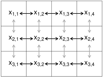
Figure 1: Example of a $3\times 4$ grid of pixels with 9 horizontal differences marked by black arrows and 8 vertical differences in grey. The total number of first order nearest neighbor differences is 17.

Model (2) incorporates a Laplace penalization that is expressed making use of the auxiliary variables $b_{j}>0$, $j=1,\ldots,d$, and the following result.

Result 1.

Let $x$ and $b$ be random variables such that

$$x\,|\,b\sim N\left(0,\sigma^{2}/b\right)\quad\mbox{and}\quad b\sim\mbox{Inverse-$\chi^{2}$}\left(2,1\right),\quad\mbox{with}\quad\sigma>0.$$

Then $x\sim\mbox{Laplace}\left(0,\sigma\right)$.

The design of the kernel matrix $\boldsymbol{K}$ varies according to the inverse problem characteristics. As illustration and for later use on real biomedical data we consider a Gaussian kernel matrix $\boldsymbol{K}$ and show its application to a simple unidimensional problem. If $\boldsymbol{y}$ is a vector of $m$ recordings from a unidimensional space having one-to-one correspondence with $\boldsymbol{x}$, the $(i,j)$th entry of a Gaussian kernel matrix $\boldsymbol{K}$ is given as follows:

$$K_{ij}=(2\pi\delta^{2})^{-1/2}\exp\{-(i-j)^{2}/(2\delta^{2})\},\quad i=1,\ldots,m,\quad j=1,\ldots,m,$$ (5)

where $\delta>0$ is a parameter that governs the amount of blur. For illustration, consider the Blocks test function (Donoho and Johnstone, 1994; Nason, 2008) from the wavethresh package (Nason, 2013) available in R (R Core Team, 2021). The piecewise constant nature of this function makes estimation a very challenging problem especially when tackled as an inverse problem, but it is well motivated by stratigraphy problems in archaeology (Allum et al., 1999; Aykroyd et al., 2001). Figure 2 shows three examples produced through (1) and the Gaussian kernel (5), with $m=100$, $\sigma=1$ and $\delta=0,2,5$. In each plot the red dashed line shows the true Blocks function to estimate. In the plot corresponding to $\delta=0$ blurring is not added to the generation process and the data points are randomly scattered around the true function. Blurring is introduced when $\delta>0$ and points scatter around a rounded solid line. The cases where $\delta=2$ and $\delta=5$ respectively correspond to moderate and large blurring of the underlying true function and hence moderate and difficult inverse problems.

Figure 2: Data points obtained through the Blocks test function (red dashed line) along with blurred test function (solid line) for different levels of blur: no blur ($\delta=0$), moderate blur ($\delta=2$) and large blur ($\delta=5$).

In two dimensions, assuming the observed data is stored in a matrix $\boldsymbol{Y}$, each element of a Gaussian kernel matrix $\boldsymbol{K}$ links an element of $\boldsymbol{y}=\mathop{\mbox{\rm vec}}(\boldsymbol{Y})$ with one of $\boldsymbol{x}=\mathop{\mbox{\rm vec}}(\boldsymbol{X})$. The entry of $\boldsymbol{K}$ corresponding to a pair $(Y_{ij},X_{i^{\prime}j^{\prime}})$ is given by

$$(2\pi\delta^{2})^{-1}\exp[-\{(i-i^{\prime})^{2}+(j-j^{\prime})^{2}\}/(2\delta^{2})],\quad\mbox{for }\delta>0.$$ (6)

The effect of $\delta$ on blurring is analogous to the one described for unidimensional problems.

The kernel matrix we adopt for the illustration on archaeological data has a more complicated definition and relies upon the spread function defined in Section 2 of Aykroyd et al. (2001). The spread function models magnetic anomalies and depends on latitude and longitude of the archaeological site on the Earth’s surface, the geometry of the gradiometer used to survey the area and the site physical properties. Further details about the design of $\boldsymbol{K}$ for archaeological data are provided in the supplementary information.

3 Model Fitting via Variational Methods

In this section, we study variational Bayes approximations, namely mean field variational Bayes (MFVB) and variational message passing (VMP), for fitting the base model (2). Emphasis is placed onto the message passing on factor graph fragment prescription, which provides the infrastructure for compartmentalized and scalable algorithm implementations.

For studying MFVB and VMP note that the joint density function of all the random variables and random vectors in model (2) admits the following factorization:

$$p\left(\boldsymbol{y},\boldsymbol{x},\boldsymbol{b},\sigma^{2}_{\varepsilon},\sigma^{2}_{x},a_{\varepsilon},a_{x}\right)=p\left(\boldsymbol{y}|\boldsymbol{x},\sigma^{2}_{\varepsilon}\right)p\left(\boldsymbol{x}|\boldsymbol{b},\sigma^{2}_{x}\right)p\left(\boldsymbol{b}\right)p\left(\sigma^{2}_{\varepsilon}|a_{\varepsilon}\right)p\left(\sigma^{2}_{x}|a_{x}\right)p\left(a_{\varepsilon}\right)p\left(a_{x}\right).$$ (7)

Both variational inference procedures are based upon approximating the joint posterior density function through a product of approximating density functions. A possible mean field restriction on the joint posterior density function of all parameters in (2) is

$$p\left(\boldsymbol{x},\boldsymbol{b},\sigma^{2}_{\varepsilon},\sigma_{x}^{2},a_{\varepsilon},a_{x}|\boldsymbol{y}\right)\approx q\left(\boldsymbol{x}\right)q\left(\sigma^{2}_{\varepsilon}\right)q\left(\sigma^{2}_{x}\right)q\left(a_{\varepsilon}\right)q\left(a_{x}\right)\prod_{j=1}^{d}q_{j}\left(b_{j}\right).$$ (8)

Typically, more restrictive density products facilitate the derivation of a variational algorithm but also negatively impact on the quality of the approximation. On the other hand, less severe restrictions may increase algebraic and computational complexity of the variational algorithms.

The scope of MFVB and VMP is to provide expressions for the optimal $q$-densities that minimize the Kullback–Leibler divergence between the approximating densities themselves and the left-hand side of (8). The former is based upon a directed acyclic graph interpretation of the model, whereas the latter benefits from a factor graph representation and its subsequent division into factor graph fragments. Both strategies reach the same final approximation by construction. Details for fitting model (2) under restriction (8) via MFVB and VMP are shown in Sections 3.1 and 3.2.

3.1 Mean Field Variational Bayes

Mean field variational Bayes is a well established approximate Bayesian inference technique where tractability is achieved through factorization of the approximating density. We refer the reader to Section 3 of Wand et al. (2011) for fuller details on MFVB implementation.

Figure 3 is a directed acyclic graph representation of model (2), where the shaded circle corresponds to the observed data, the unshaded circles correspond to model parameters and auxiliary variables, and the small solid circles are used for hyperparameters.

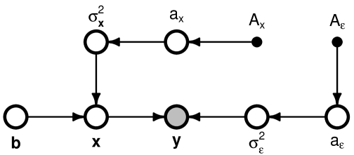
Figure 3: Directed acyclic graph representation of the Normal response model with Laplace penalization in (2). The shaded circle corresponds to the observed data. The unshaded circles correspond to model parameters and auxiliary variables. The small solid circles correspond to hyperparameters.

Referring to restriction (8) , the MFVB approximations to the posterior density functions of the parameters and auxiliary variables depicted in the directed acyclic graph have the following optimal forms:

$$q^{*}(\boldsymbol{x})\,\text{is a}\,N\big{(}\boldsymbol{\mu}_{q\left(\boldsymbol{x}\right)},\boldsymbol{\Sigma}_{q\left(\boldsymbol{x}\right)}\big{)}\,\text{density function},$$ (9)

$$q^{*}(b_{j})\,\text{is an}\,\text{Inverse-Gaussian}\big{(}\mu_{q(b_{j})},\lambda_{q(b_{j})}\big{)}\,\text{density function, for}\,j=1,\ldots,d,$$ (10)

$$q^{*}(\sigma^{2}_{\varepsilon})\,\mbox{is an}\,\mbox{Inverse-}\chi^{2}\left(\kappa_{q\left(\sigma^{2}_{\varepsilon}\right)},\lambda_{q\left(\sigma^{2}_{\varepsilon}\right)}\right)\,\text{density function},$$ (11)

$$q^{*}(\sigma^{2}_{x})\,\mbox{is an}\,\mbox{Inverse-}\chi^{2}\big{(}\kappa_{q\left(\sigma^{2}_{x}\right)},\lambda_{q\left(\sigma^{2}_{x}\right)}\big{)}\,\text{density function},$$ (12)

$$q^{*}(a_{\varepsilon})\,\mbox{is an}\,\mbox{Inverse-}\chi^{2}\big{(}\kappa_{q\left(a_{\varepsilon}\right)},\lambda_{q\left(a_{\varepsilon}\right)}\big{)}\,\text{density function}$$ (13)

and $$q^{*}(a_{x})\,\mbox{is an}\,\mbox{Inverse-}\chi^{2}\big{(}\kappa_{q\left(a_{x}\right)},\lambda_{q\left(a_{x}\right)}\big{)}\,\text{density function}.$$ (14)

Details about the optimal density function parameters are given in the supplementary information. Such parameters can be obtained through the MFVB iterative scheme listed as Algorithm 1.

• Data Inputs: $\boldsymbol{y}$ $(m\times 1)$, $\boldsymbol{K}$ $(m\times m)$.

• Hyperparameter Inputs: $A_{\varepsilon}>0$, $A_{x}>0$.

• Initialize: $\mu_{q\left(1/\sigma^{2}_{\varepsilon}\right)}>0$, $\mu_{q\left(1/\sigma^{2}_{x}\right)}>0$, $\mu_{q\left(1/a_{\varepsilon}\right)}>0$, $\mu_{q\left(1/a_{x}\right)}>0$, $\boldsymbol{\mu}_{q(\boldsymbol{b})}$ $(d\times 1)$ vector of
               positive elements.

• $\kappa_{q\left(\sigma^{2}_{\varepsilon}\right)}\longleftarrow m+1\quad;\quad\kappa_{q\left(\sigma^{2}_{x}\right)}\longleftarrow d+1\quad;\quad\kappa_{q\left(a_{\varepsilon}\right)}\longleftarrow 2\quad;\quad\kappa_{q\left(a_{x}\right)}\longleftarrow 2$.

• Cycle:

  • $\boldsymbol{\Sigma}_{q\left(\boldsymbol{x}\right)}\longleftarrow\left(\mu_{q(1/\sigma^{2}_{\varepsilon})}\boldsymbol{K}^{T}\boldsymbol{K}+\mu_{q(1/\sigma^{2}_{x})}\boldsymbol{L}^{T}\mathop{\mbox{\rm diag}}(\boldsymbol{\mu}_{q(\boldsymbol{b})})\boldsymbol{L}\right)^{-1}$

  • $\boldsymbol{\mu}_{q\left(\boldsymbol{x}\right)}\longleftarrow\mu_{q(1/\sigma_{\varepsilon}^{2})}\boldsymbol{\Sigma}_{q\left(\boldsymbol{x}\right)}\boldsymbol{K}^{T}\boldsymbol{y}$

  • $\lambda_{q\left(\sigma^{2}_{\varepsilon}\right)}\longleftarrow\mu_{q(1/a_{\varepsilon})}+\|\boldsymbol{y}-\boldsymbol{K}\boldsymbol{\mu}_{q\left(\boldsymbol{x}\right)}\|^{2}+\mbox{tr}\left(\boldsymbol{K}^{T}\boldsymbol{K}\boldsymbol{\Sigma}_{q\left(\boldsymbol{x}\right)}\right)$

  • $\mu_{q\left(1/\sigma^{2}_{\varepsilon}\right)}\longleftarrow\kappa_{q\left(\sigma^{2}_{\varepsilon}\right)}/\lambda_{q\left(\sigma^{2}_{\varepsilon}\right)}$

  • $\lambda_{q\left(a_{\varepsilon}\right)}\longleftarrow\mu_{q(1/\sigma^{2}_{\varepsilon})}+1/A_{\varepsilon}^{2}\quad;\quad\mu_{q(1/a_{\varepsilon})}\longleftarrow\kappa_{q\left(a_{\varepsilon}\right)}/\lambda_{q\left(a_{\varepsilon}\right)}$

  • $\boldsymbol{\tau}_{1}\longleftarrow\big{(}\boldsymbol{L}\boldsymbol{\mu}_{q\left(\boldsymbol{x}\right)}\big{)}^{2}+\mathop{\mbox{\rm diagonal}}(\boldsymbol{L}\boldsymbol{\Sigma}_{q\left(\boldsymbol{x}\right)}\boldsymbol{L}^{T})$

  • $\lambda_{q\left(\sigma^{2}_{x}\right)}\longleftarrow\mu_{q(1/a_{x})}+\mu_{q\left(\boldsymbol{b}\right)}^{T}\boldsymbol{\tau}_{1}$

  • $\mu_{q\left(1/\sigma^{2}_{x}\right)}\longleftarrow\kappa_{q\left(\sigma^{2}_{x}\right)}/\lambda_{q\left(\sigma^{2}_{x}\right)}$

  • $\lambda_{q\left(a_{x}\right)}\longleftarrow\mu_{q(1/\sigma^{2}_{x})}+1/A_{x}^{2}\quad;\quad\mu_{q(1/a_{x})}\longleftarrow\kappa_{q\left(a_{x}\right)}/\lambda_{q\left(a_{x}\right)}$

  • $\boldsymbol{\tau}_{2}\longleftarrow\mu_{q\left(1/\sigma^{2}_{x}\right)}\boldsymbol{\tau}_{1}\quad;\quad\boldsymbol{\mu}_{q\left(\boldsymbol{b}\right)}\longleftarrow 1/\sqrt{\boldsymbol{\tau}_{2}}$

• Output: $\boldsymbol{\mu}_{q\left(\boldsymbol{x}\right)}$, $\boldsymbol{\Sigma}_{q\left(\boldsymbol{x}\right)}$, $\boldsymbol{\mu}_{q\left(\boldsymbol{b}\right)}$, $\boldsymbol{\lambda}_{q\left(\boldsymbol{b}\right)}\equiv\boldsymbol{1}_{d}$, $\kappa_{q\left(\sigma^{2}_{\varepsilon}\right)}$, $\lambda_{q\left(\sigma^{2}_{\varepsilon}\right)}$, $\kappa_{q\left(\sigma^{2}_{x}\right)}$, $\lambda_{q\left(\sigma^{2}_{x}\right)}$, $\kappa_{q\left(a_{\varepsilon}\right)}$, $\lambda_{q\left(a_{\varepsilon}\right)}$, $\kappa_{q\left(a_{x}\right)}$, $\lambda_{q\left(a_{x}\right)}$.

Algorithm 1 Mean field variational Bayes scheme for fitting the inverse problem model (2), using product density restriction (7).

3.2 Variational Message Passing

A detailed description of VMP as a method for fitting statistical models that have a factor graph representation is provided in Sections 2–4 of Wand (2017). The same notational conventions of Wand (2017) concerning message passing are used in this work and briefly summarized here.

A factor graph is an ensemble of factors connected to stochastic nodes by edges. Let $f$ denote a generic factor and function of one or more stochastic nodes, and $\theta$ be a generic stochastic variable represented by a node. If $\theta$ is a neighbor of $f$ in the factor graph, then the messages passed from $f$ to $\theta$ and from $\theta$ to $f$ are functions of $\theta$ and are denoted by $m_{\tiny f\rightarrow\theta}(\theta)$ and $m_{\tiny\theta\rightarrow f}(\theta)$, respectively. These messages are typically proportional to an exponential family density function and so are such that

$$m_{\tiny f\rightarrow\theta}(\theta)\propto\exp\big{\{}\boldsymbol{T}(\theta)^{T}\mbox{\large$\boldsymbol{\eta}$}_{\tiny f\rightarrow\theta}\big{\}}\quad\mbox{and}\quad m_{\tiny\theta\rightarrow f}(\theta)\propto\exp\big{\{}\boldsymbol{T}(\theta)^{T}\mbox{\large$\boldsymbol{\eta}$}_{\tiny\theta\rightarrow f}\big{\}},$$

where $\boldsymbol{T}(\theta)$ is a sufficient statistic vector, and $\mbox{\large$\boldsymbol{\eta}$}_{\tiny f\rightarrow\theta}$ and $\mbox{\large$\boldsymbol{\eta}$}_{\tiny\theta\rightarrow f}$ are the message natural parameter vectors. Expressions (7)–(9) of Wand (2017) show how both messages can be obtained for given factors and nodes. For each parameter $\theta$, the optimal approximating density $q^{*}(\theta)$ belongs to an exponential family with natural parameter vector

$$\mbox{\large$\boldsymbol{\eta}$}_{\tiny q(\theta)}\equiv\mbox{\large$\boldsymbol{\eta}$}_{\tiny f\rightarrow\theta}+\mbox{\large$\boldsymbol{\eta}$}_{\tiny\theta\rightarrow f}.$$

The notion of a factor graph fragment, or simply fragment, allows for compartmentalization of algebra and computer code and we exploited it to fit inverse problems via VMP.

The corresponding factor graph representation of (7) given the density product restriction (8) appears in Figure 4. Colors mark different fragment types, in accordance with the nomenclature presented in Wand (2017) for variational message passing on factor graph fragments and numbers label seven factor graph fragments. Some of these have been studied in previous works.

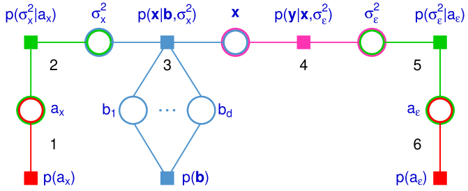
Figure 4: Factor graph representation of the Normal response model with Laplace penalization in (2), where the square nodes correspond to the density functions, or factors, at the right-hand side of (7). The circular nodes correspond to stochastic nodes of the $q$-density factorization in (8). The fragments are numbered 1 to 6, whereas colors identify different fragments types.

Those numbered 1, 2, 5 and 6 are already catalogued in Maestrini and Wand (2021) as Inverse G-Wishart prior fragment (1 and 6) and iterated Inverse G-Wishart fragment (2 and 5). Fragment number 4 corresponds to the Gaussian likelihood fragment treated in Section 4.1.5 of Wand (2017), whose notation can be aligned with that of model (2) by settings $\boldsymbol{A}$, $\boldsymbol{\theta}_{1}$ and $\theta_{2}$ equal to the current $\boldsymbol{K}$, $\boldsymbol{x}$ and $\sigma^{2}_{\varepsilon}$, respectively. In the view of VMP, we can just read off from equations (38) and (39) of Wand (2017) and get the following updates for fragment 5:

$$\mbox{\large$\boldsymbol{\eta}$}_{\mbox{\footnotesize$p(\boldsymbol{y}|\boldsymbol{x},\sigma^{2}_{\varepsilon})\rightarrow\boldsymbol{x}$}}\longleftarrow\left[\begin{array}[]{c}\boldsymbol{K}^{T}\boldsymbol{y}\\[4.30554pt] -\frac{1}{2}\mathop{\mbox{\rm vec}}\left(\boldsymbol{K}^{T}\boldsymbol{K}\right)\end{array}\right]\Big{\{}\left(\mbox{\large$\boldsymbol{\eta}$}_{\mbox{\footnotesize$p(\boldsymbol{y}|\,\boldsymbol{x},\sigma^{2}_{\varepsilon})\leftrightarrow\sigma^{2}_{\varepsilon}$}}\right)_{1}+1\Big{\}}\Big{/}\Big{\{}\left(\mbox{\large$\boldsymbol{\eta}$}_{\mbox{\footnotesize$p(\boldsymbol{y}|\,\boldsymbol{x},\sigma^{2}_{\varepsilon})\leftrightarrow\sigma^{2}_{\varepsilon}$}}\right)_{2}\Big{\}}$$

and

$$\mbox{\large$\boldsymbol{\eta}$}_{\mbox{\footnotesize$p(\boldsymbol{y}|\boldsymbol{x},\sigma^{2}_{\varepsilon})\rightarrow\sigma^{2}_{\varepsilon}$}}\longleftarrow\left[\begin{array}[]{c}-n/2\\[4.30554pt] G_{\tiny{\mbox{VMP}}}\left(\mbox{\large$\boldsymbol{\eta}$}_{\mbox{\footnotesize$p(\boldsymbol{y}|\,\boldsymbol{x},\sigma^{2}_{\varepsilon})\leftrightarrow\boldsymbol{x}$}};\boldsymbol{K}^{T}\boldsymbol{K},\boldsymbol{K}^{T}\boldsymbol{y},\boldsymbol{y}^{T}\boldsymbol{y}\right)\end{array}\right],$$

where the function $G_{\tiny{\mbox{VMP}}}$ is defined in Section 2.7 of Wand (2017).

New calculations are needed only for fragment 3 to compose a VMP algorithm for the whole model. Factor $p\left(\boldsymbol{b}\right)$ symbolizes the specification

$$b_{j}\stackrel{{\scriptstyle{\tiny\mbox{ind.}}}}{{\sim}}\mbox{Inverse-$\chi^{2}$}\left(2,1\right),\quad j=1,\ldots,d,$$ (15)

but may also represent other penalizations. Examples of alternative shrinkage distributions are displayed in Table 1 and discussed in Section 3.3.

The factor $p\left(x|\boldsymbol{b},\sigma^{2}_{x}\right)$ of fragment 3 corresponds to the possibly improper specification (3). The logarithm of this likelihood factor is

$$\log p\left(x|\boldsymbol{b},\sigma^{2}_{x}\right)=-\frac{d}{2}\log\left(\sigma^{2}_{x}\right)-\frac{1}{2\sigma^{2}_{x}}\boldsymbol{x}^{T}\boldsymbol{L}^{T}\mathop{\mbox{\rm diag}}\left(b\right)\boldsymbol{L}\boldsymbol{x}+\frac{1}{2}\sum_{i=1}^{d}\log\left(b_{i}\right)+\mbox{const}.$$ (16)

Combining (16) with the auxiliary variable distributional assumption in (15) we get the VMP scheme listed as Algorithm 2 for fitting the penalization part of model (2).

• Inputs: $\mbox{\large$\boldsymbol{\eta}$}_{\mbox{\footnotesize$p(\boldsymbol{x}|\boldsymbol{b},\sigma^{2}_{x})\rightarrow\boldsymbol{x}$}}$, $\mbox{\large$\boldsymbol{\eta}$}_{\mbox{\footnotesize$\boldsymbol{x}\rightarrow p(\boldsymbol{x}|\,\boldsymbol{b},\sigma^{2}_{x})$}}$, $\mbox{\large$\boldsymbol{\eta}$}_{\mbox{\footnotesize$p(\boldsymbol{x}|\,\boldsymbol{b},\sigma^{2}_{x})\rightarrow\sigma^{2}_{x}$}}$, $\mbox{\large$\boldsymbol{\eta}$}_{\mbox{\footnotesize$\sigma^{2}_{x}\rightarrow p(\boldsymbol{x}|\,\boldsymbol{b},\sigma^{2}_{x})$}}$.

• Updates:

  • $\mu_{q\left(1/\sigma^{2}_{x}\right)}\longleftarrow\Big{\{}\left(\mbox{\large$\boldsymbol{\eta}$}_{\mbox{\footnotesize$p(\boldsymbol{x}|\,\boldsymbol{b},\sigma^{2}_{x})\leftrightarrow\sigma^{2}_{x}$}}\right)_{1}+1\Big{\}}\Big{/}\Big{\{}\left(\mbox{\large$\boldsymbol{\eta}$}_{\mbox{\footnotesize$p(\boldsymbol{x}|\,\boldsymbol{b},\sigma^{2}_{x})\leftrightarrow\sigma^{2}_{x}$}}\right)_{2}\Big{\}}$

  • $\boldsymbol{\Omega}_{1}\longleftarrow-\frac{1}{2}\left\{\mathop{\mbox{\rm vec}}^{-1}\left(\left(\mbox{\large$\boldsymbol{\eta}$}_{\mbox{\footnotesize$p(\boldsymbol{x}|\,\boldsymbol{b},\sigma^{2}_{x})\leftrightarrow\boldsymbol{x}$}}\right)_{2}\right)\right\}^{-1}$

  • $\boldsymbol{\omega}_{2}\longleftarrow\boldsymbol{\Omega}_{1}\left(\mbox{\large$\boldsymbol{\eta}$}_{\mbox{\footnotesize$p(\boldsymbol{x}|\,\boldsymbol{b},\sigma^{2}_{x})\leftrightarrow\sigma^{2}_{x}$}}\right)_{1}\quad;\quad\boldsymbol{\omega}_{3}\longleftarrow\boldsymbol{L}\boldsymbol{\omega}_{2}\quad;\quad\boldsymbol{\omega}_{4}\longleftarrow\mathop{\mbox{\rm diagonal}}\left(\boldsymbol{L}\boldsymbol{\Omega}_{1}\boldsymbol{L}^{T}\right)$

  • $\boldsymbol{\omega}_{5}\longleftarrow\boldsymbol{\omega}_{3}^{2}+\boldsymbol{\omega}_{4}\quad;\quad\boldsymbol{\omega}_{6}\longleftarrow\mu_{q\left(1/\sigma^{2}_{x}\right)}\boldsymbol{\omega}_{5}$

  • $\boldsymbol{\mu}_{q\left(\boldsymbol{b}\right)}\longleftarrow 1/\sqrt{\boldsymbol{\omega}_{6}}\quad;\quad\boldsymbol{\Omega}_{7}\longleftarrow\boldsymbol{L}^{T}\mathop{\mbox{\rm diag}}\left(\mu_{q\left(\boldsymbol{b}\right)}\right)\boldsymbol{L}$

• until convergence.

• Outputs:

  $\quad\mbox{\large$\boldsymbol{\eta}$}_{\mbox{\footnotesize$p(\boldsymbol{x}|\boldsymbol{b},\sigma^{2}_{x})\rightarrow\boldsymbol{x}$}}\longleftarrow\mu_{q\left(1/\sigma^{2}_{x}\right)}\left[\begin{array}[]{c}\boldsymbol{0}\\[3.87498pt] -\frac{1}{2}\mathop{\mbox{\rm vec}}\left(\boldsymbol{\Omega}_{7}\right)\end{array}\right]\quad;\quad\mbox{\large$\boldsymbol{\eta}$}_{\mbox{\footnotesize$p(\boldsymbol{x}|\,\boldsymbol{b},\sigma^{2}_{x})\rightarrow\sigma^{2}_{x}$}}\longleftarrow-\frac{1}{2}\left[\begin{array}[]{c}m_{L}\\[3.87498pt] \mu_{q\left(\boldsymbol{b}\right)}^{T}\boldsymbol{\omega}_{5}\end{array}\right].$

Algorithm 2 Variational message passing inputs, updates and outputs of the penalization likelihood fragment given by (3) and (15), and corresponding to factor graph fragment 3 of Figure 4.

The combination of Algorithm 2 with the Inverse G-Wishart fragment algorithms of Maestrini and Wand (2021) and the Gaussian likelihood fragment algorithm of Wand (2017) gives rise to a full VMP procedure for fitting and approximate inference on model (2). Complete details about the implementation of VMP for fitting the inverse problem model (2) are provided in the supplementary information.

3.3 Alternative Response and Penalization Distributions

The message passing on factor graph fragments paradigm allows for flexible imposition of non-Normal response distributions. Fragment 5 of Figure 4 can be replaced by one of the likelihood fragments identified in Nolan and Wand (2017), Maestrini and Wand (2018) or McLean and Wand (2019) to accommodate a variety of response distributions such as, for instance, binary-logistic, Poisson, Negative Binomial, $t$, Asymmetric Laplace, Skew Normal, Skew $t$ and Finite Normal Mixtures.

Other penalization structures can be easily incorporated by varying the distributional assumption on the vector of auxiliary variables $\boldsymbol{b}$. Neville et al. (2014) studied MFVB inference for three continuous sparse signal shrinkage distributions, namely the Horseshoe, Negative-Exponential-Gamma and Generalized Double Pareto distributions, that can replace the Laplace penalization employed in model (2). References for the development of these sparse shrinkage priors are respectively Carvalho et al. (2010), Griffin and Brown (2011) and Armagan et al. (2013).

The derivation of variational algorithms for models containing these shrinkage distributions can be quite challenging. In fact, the variational algorithm algebraic complexity and inference performance rely upon an accurate choice of their auxiliary variable representations. Neville et al. (2014) propose two alternative auxiliary variable representations for each of the aforementioned shrinkage distributions by making use of either one or two sets of auxiliary variables. Their empirical and theoretical evidence show the supremacy of representations based on a single set of auxiliary variables in terms of posterior density approximation and computational complexity for all three cases. If this auxiliary variable representation is chosen, then the three penalizations can be easily imposed in model (2) and replace the Laplace distribution by simply modifying the distributional assumption on the auxiliary vector $\boldsymbol{b}$. Algorithms 1 and 2 can still be used by simple replacement of the update for $\boldsymbol{\mu}_{q\left(\boldsymbol{b}\right)}$ with one of those listed in the last column of Table 1. Some expressions in Table 1 related to the Negative-Exponential-Gamma and Generalized Double Pareto cases depend on the parabolic cylinder function of order $\nu$, $\mathcal{D}_{\nu}(x)$, and $\mathcal{R}_{\nu}(x)\equiv\mathcal{D}_{-\nu-2}(x)/\mathcal{D}_{-\nu-1}(x)$, for $\nu>0$ and $x>0$. Efficient computation of function $\mathcal{R}_{\nu}(x)$ is discussed in Appendix A of Neville et al. (2014).

Several other penalizations can be imposed on the base inverse problem model. The penalization in model (2) is a particular case of the Bayesian lasso of Park and Casella (2008) that makes use of a Gamma prior on the Laplace squared scale parameter. Tung et al. (2019) show the use of MFVB for variable selection in generalized linear mixed models via Bayesian adaptive lasso. Ormerod et al. (2017) develop a MFVB approximation to a linear model with a spike-and-slab prior on the regression coefficients. A detailed discussion on variable selection priors and variational inference fitting goes beyond the scope of this article. However, for the analysis of archaeological data of Section 6 we show how the Laplace penalization can be easily replaced by a Horseshoe prior without deriving a VMP algorithm from scratch. In the same real data analysis we replace the Normal response assumption with a Skew Normal one aiming to show the flexibility of our approach rather than recommending a particular distribution as being the best.

Penalization	Density function	MFVB or VMP update
Horseshoe	$p\left(b_{j}\right)=\pi^{-1}b_{j}^{-1/2}\left(1+b_{j}\right)^{-1}$	$\boldsymbol{\mu}_{q\left(\boldsymbol{b}\right)}\longleftarrow\frac{2}{\boldsymbol{\zeta}\odot\exp\left(\frac{1}{2}\boldsymbol{\zeta}\right)\odot E_{1}\left(\frac{1}{2}\boldsymbol{\zeta}\right)}-1$
Negative-	$p\left(b_{j}\right)=\lambda b_{j}^{\lambda-1}\left(1+b_{j}\right)^{-\lambda-1}$	$\boldsymbol{\mu}_{q\left(\boldsymbol{b}\right)}\longleftarrow(2\lambda+1)\mathcal{R}_{2\lambda}\left(\sqrt{\boldsymbol{\zeta}}\right)\odot\sqrt{\boldsymbol{\zeta}}$
Exponential-Gamma
Generalized	$p\left(b_{j}\right)=\frac{1}{2}\left(1+\lambda\right)\lambda^{1+\lambda}$	$\boldsymbol{\mu}_{q\left(\boldsymbol{b}\right)}\longleftarrow\frac{\sqrt{2}\left(\lambda+1\right)}{\sqrt{\boldsymbol{\zeta}}\odot(\sqrt{2}\lambda+\boldsymbol{\zeta})}$
Double Pareto	$\times b_{j}^{\left(\lambda-2\right)/2}e^{\lambda^{2}b_{j}/4}\mathcal{D}_{-\lambda-2}\left(\lambda\sqrt{b_{j}}\right)$

Table 1: Distributions of the auxiliary variables $b_{j}>0$, $j=1\ldots d$, that produce the penalizations analyzed in Neville et al. (2014) when introduced in model (2) in lieu of the Laplace penalization. Here the shape parameter $\lambda>0$ is fixed. For each distribution, the MFVB or VMP update for $\boldsymbol{\mu}_{q\left(\boldsymbol{b}\right)}$ is displayed in the last column. When using Algorithm 1 for MFVB, set $\boldsymbol{\zeta}\equiv\boldsymbol{\tau}_{2}$; when using Algorithm 2 for VMP, set $\boldsymbol{\zeta}\equiv\boldsymbol{\omega}_{6}$.

4 Streamlined Variational Algorithm Updates

In typical inverse problem applications the number of observations can be very high and a naïve implementation of Algorithms 2 and 1 may lead to a bottleneck due to operations involving a large contrast matrix $\boldsymbol{L}$ and big matrix inversion steps related to $\boldsymbol{K}$. However, the structure of matrices $\boldsymbol{L}$ and $\boldsymbol{K}$ is such that computationally expensive algorithm updates may be efficiently performed. In this section we propose solutions to simplify algorithm updates and reduce their computational complexity. The results shown here are designed for one- and two-dimensional problems but are applicable to extensions to higher dimensions.

4.1 Removal of the Contrast Matrix

The contrast matrix $\boldsymbol{L}$ is a potentially massive sparse matrix that one does not want to compute or store. The number of rows of $\boldsymbol{L}$ is given by the $d$ differences between the elements of $\boldsymbol{x}$ considered, whereas the number of columns is given by the length $m$ of $\boldsymbol{x}$. For one-dimensional problems with a first nearest neighbor structure only the two longest diagonals of $\boldsymbol{L}$ have non-zero elements, as shown in (4). The contrast matrix of two-dimensional problems under the same assumptions is sparse and has number of non-zero elements equal to twice the number of differences between elements of $\boldsymbol{x}$, that is $2d$.

The updates of the variational Algorithms 1 and 2 that make use of matrix $\boldsymbol{L}$ have the following form:

$$\boldsymbol{L}\boldsymbol{v},\mbox{ where }\boldsymbol{v}\mbox{ is a vector};$$ (17)

$$\mathop{\mbox{\rm diagonal}}(\boldsymbol{L}\boldsymbol{M}\boldsymbol{L}^{T}),\mbox{ where }\boldsymbol{M}\mbox{ is a symmetric positive definite matrix};$$ (18)

$$\boldsymbol{L}^{T}\mathop{\mbox{\rm diag}}(\boldsymbol{w})\boldsymbol{L},\mbox{ where }\boldsymbol{w}\mbox{ is a vector}.$$ (19)

The ensuing lemmas allow efficient computation of the MFVB and VMP updates that utilise matrix $\boldsymbol{L}$ in the forms described in (17)–(19). One- and two-dimensional problems are considered. The results for two dimensions identify a framework which is extendible to higher dimensions.

4.1.1 One-dimensional Case

Consider a one-dimensional inverse problem analyzed via model (2) and suppose $\boldsymbol{x}$ has one-to-one correspondence with a sequence of hidden and equispaced locations on a line. Assume first nearest neighbor differences are modeled via the contrast matrix $\boldsymbol{L}_{\mbox{\tiny 1D}}$ defined in (4). Then matrix $\boldsymbol{L}$ can be removed from (17) by making use of the following lemma.

Lemma 1.

Let $\boldsymbol{v}$ be a vector of length $d_{\mbox{\tiny$\boldsymbol{v}$}}$ and $\boldsymbol{L}_{\mbox{\tiny 1D}}$ a $\left(d_{\mbox{\tiny$\boldsymbol{v}$}}-1\right)\times d_{\mbox{\tiny$\boldsymbol{v}$}}$ matrix having form (4). Then

$$\boldsymbol{L}_{\mbox{\tiny 1D}}\boldsymbol{v}=\left[\begin{array}[]{c}v_{2}-v_{1}\\ v_{3}-v_{2}\\ \vdots\\ v_{d_{\mbox{\tiny$\boldsymbol{v}$}}}-v_{d_{\mbox{\tiny$\boldsymbol{v}$}}-1}\end{array}\right],$$

which is a vector of length $d_{\mbox{\tiny$\boldsymbol{v}$}}-1$.

We can get rid of matrix $\boldsymbol{L}$ from expressions having form (18) through the next lemma.

Lemma 2.

Let $\boldsymbol{M}$ be a symmetric $d_{\mbox{\tiny$\boldsymbol{M}$}}\times d_{\mbox{\tiny$\boldsymbol{M}$}}$ matrix and $\boldsymbol{L}_{\mbox{\tiny 1D}}$ a $\left(d_{\mbox{\tiny$\boldsymbol{M}$}}-1\right)\times d_{\mbox{\tiny$\boldsymbol{M}$}}$ matrix having form (4). Then for $i=1,\ldots,d_{\mbox{\tiny$\boldsymbol{M}$}}-1$,

$$\left(\boldsymbol{L}_{\mbox{\tiny 1D}}\boldsymbol{M}\boldsymbol{L}_{\mbox{\tiny 1D}}^{T}\right)_{ii}=M_{i+1,i+1}-2M_{i+1,i}+M_{i,i}$$

or, equivalently,

$$\mathop{\mbox{\rm diagonal}}\left(\boldsymbol{L}_{\mbox{\tiny 1D}}\boldsymbol{M}\boldsymbol{L}_{\mbox{\tiny 1D}}^{T}\right) =\mathop{\mbox{\rm diagonal}}\left(\boldsymbol{M}\right)_{2:d_{\mbox{\tiny$\boldsymbol{M}$}}}+\mathop{\mbox{\rm diagonal}}\left(\boldsymbol{M}\right)_{1:\left(d_{\mbox{\tiny$\boldsymbol{M}$}}-1\right)}$$

$$\quad-2\,\mathop{\mbox{\rm diagonal}}\left(\boldsymbol{M}_{2:d_{\mbox{\tiny$\boldsymbol{M}$}},1:\left(d_{\mbox{\tiny$\boldsymbol{M}$}}-1\right)}\right),$$

which is a vector of length $d_{\mbox{\tiny$\boldsymbol{M}$}}-1$.

The following lemma simplifies the computation of (19).

Lemma 3.

Let $\boldsymbol{w}$ be a vector of length $d_{\mbox{\tiny$\boldsymbol{w}$}}$ and $\boldsymbol{L}_{\mbox{\tiny 1D}}$ a $\left(d_{\mbox{\tiny$\boldsymbol{w}$}}-1\right)\times d_{\mbox{\tiny$\boldsymbol{w}$}}$ matrix having form (4). Then

$$\boldsymbol{L}_{\mbox{\tiny 1D}}^{T}\mathop{\mbox{\rm diag}}\left(\boldsymbol{w}\right)\boldsymbol{L}_{\mbox{\tiny 1D}}=\mathop{\mbox{\rm tridiag}}\left(\left[\begin{array}[]{c}w_{1}\\ \boldsymbol{w}_{1:\left(d_{\mbox{\tiny$\boldsymbol{w}$}}-1\right)}+\boldsymbol{w}_{2:d_{\mbox{\tiny$\boldsymbol{w}$}}}\\ w_{d_{\mbox{\tiny$\boldsymbol{w}$}}}\end{array}\right],-\boldsymbol{w}\right),$$

which is a matrix of size $d_{\mbox{\tiny$\boldsymbol{w}$}}\times d_{\mbox{\tiny$\boldsymbol{w}$}}$.

In the R computing environment Lemmas 1–3 can be implemented with standard base functions. In particular, the function diff(v) automatically produces the result stated in Lemma 1. The expressions originated by Lemmas 2 and 3 can be visualized through the examples provided in the supplementary information.

4.1.2 Two-dimensional Case

Consider the study of bidimensional inverse problems through model (2) with $\boldsymbol{x}=\mathop{\mbox{\rm vec}}(\boldsymbol{X})$ and $\boldsymbol{X}$ being an $m_{1}\times m_{2}$ matrix whose entries correspond to a regular grid of locations. Then a first nearest neighbor contrast matrix, here denoted by $\boldsymbol{L}_{\mbox{\tiny 2D}}$, can be conveniently defined as

$$\boldsymbol{L}_{\mbox{\tiny 2D}}\equiv\left[\begin{array}[]{c}\boldsymbol{L}^{\mbox{\tiny H}}\boldsymbol{C}\\ \boldsymbol{L}^{\mbox{\tiny V}}\end{array}\right],$$ (20)

which has size $d\times(m_{1}m_{2})$, with $d=d^{\mbox{\tiny H}}+d^{\mbox{\tiny V}}$, $d^{\mbox{\tiny H}}=m_{1}(m_{2}-1)$ and $d^{\mbox{\tiny V}}=(m_{1}-1)m_{2}$. The single components of $\boldsymbol{L}_{\mbox{\tiny 2D}}$ are defined as follows:

$$\boldsymbol{L}^{\mbox{\tiny H}}\equiv\boldsymbol{I}_{m_{1}}\otimes\boldsymbol{L}_{0}^{\mbox{\tiny H}}\quad\mbox{and}\quad\boldsymbol{L}^{\mbox{\tiny V}}\equiv\boldsymbol{I}_{m_{2}}\otimes\boldsymbol{L}_{0}^{\mbox{\tiny V}},$$ (21)

where $\boldsymbol{L}^{\mbox{\tiny H}}$ and $\boldsymbol{L}^{\mbox{\tiny V}}$ are matrices of size $d^{\mbox{\tiny H}}\times(m_{1}m_{2})$ and $d^{\mbox{\tiny V}}\times(m_{1}m_{2})$, respectively. Matrix $\boldsymbol{C}$ is a $m_{1}\times m_{2}$ commutation matrix such that

$$\boldsymbol{C}\mathop{\mbox{\rm vec}}(\boldsymbol{X})=\mathop{\mbox{\rm vec}}(\boldsymbol{X}^{T}).$$

Lastly, matrices $\boldsymbol{L}_{0}^{\mbox{\tiny H}}$ and $\boldsymbol{L}_{0}^{\mbox{\tiny V}}$ have the form (4) identified for the one-dimensional case, and dimensions $(m_{2}-1)\times m_{2}$ and $(m_{1}-1)\times m_{1}$, respectively. If for instance $\boldsymbol{X}$ is of size $3\times 4$ as in the example of Figure 1, then

$$\boldsymbol{L}_{0}^{\mbox{\tiny H}}=\left[\begin{array}[]{cccc}-1&1&0&0\\ 0&-1&1&0\\ 0&0&-1&1\end{array}\right]\quad\mbox{and}\quad\boldsymbol{L}_{0}^{\mbox{\tiny V}}=\left[\begin{array}[]{ccc}-1&1&0\\ 0&-1&1\end{array}\right].$$ (22)

Superscripts H and V refer to differences between pairs of locations respectively computed in a horizontal and vertical fashion, given the row-wise and column-wise orientation identified by $\boldsymbol{X}$. The explicit expression of $\boldsymbol{L}_{\mbox{\tiny 2D}}$ for a $3\times 4$ matrix of parameters $\boldsymbol{X}$ is provided in the supplementary information. For clarity, the coefficients that define the dimensions of the $\boldsymbol{L}_{\mbox{\tiny 2D}}$ matrix components are summarized in Table (2).

Notation	Description
$m_{1}$	number of rows in $\boldsymbol{X}$ (and $\boldsymbol{Y}$)
$m_{2}$	number of columns in $\boldsymbol{X}$ (and $\boldsymbol{Y}$)
$m=m_{1}\times m_{2}$	total number of elements in $\boldsymbol{X}$ (and $\boldsymbol{Y}$)
$d^{\mbox{\tiny H}}=m_{1}(m_{2}-1)$	number of horizontal differences in $\boldsymbol{X}$
$d^{\mbox{\tiny V}}=(m_{1}-1)m_{2}$	number of vertical differences in $\boldsymbol{X}$
$d=d^{\mbox{\tiny H}}+d^{\mbox{\tiny V}}$	total number of differences in $\boldsymbol{X}$

Table 2: Notation used for two-dimensional inverse problems with first nearest neighbor differences and one-to-one correspondence between $\boldsymbol{X}$ and $\boldsymbol{Y}$.

Lemmas 4–6 are extensions of Lemmas 1–3 to the two-dimensional case, provided that $\boldsymbol{L}_{\mbox{\tiny 2D}}$ has the form identified by (20)–(22). Vector and matrix dimensions are intentionally emphasized to highlight analogies with one-dimensional problems and set up a framework extendible to higher dimensions.

The next lemma simplifies the computation of expression (17) and avoids calculating and storing matrix $\boldsymbol{L}_{\mbox{\tiny 2D}}$.

Lemma 4.

Let $\boldsymbol{V}$ be a matrix of size $m_{1}\times m_{2}$, $\boldsymbol{v}=\mathop{\mbox{\rm vec}}\left(\boldsymbol{V}\right)$ a vector of length $d_{\mbox{\tiny$\boldsymbol{v}$}}=m_{1}m_{2}$ and $\boldsymbol{L}_{\mbox{\tiny 2D}}$ a matrix of size $(d^{\mbox{\tiny H}}+d^{\mbox{\tiny V}})\times d_{\mbox{\tiny$\boldsymbol{v}$}}$ having the form defined in (20)–(22) with $d^{\mbox{\tiny H}}=m_{1}(m_{2}-1)$ and $d^{\mbox{\tiny V}}=(m_{1}-1)m_{2}$. Then

$$\boldsymbol{L}_{\mbox{\tiny 2D}}\boldsymbol{v}=\left[\begin{array}[]{c}\boldsymbol{t}^{\mbox{\tiny H}}\\ \boldsymbol{t}^{\mbox{\tiny V}}\end{array}\right],$$

where

$$\boldsymbol{t}^{\mbox{\tiny H}}=\mathop{\mbox{\rm stack}}_{i=1,\ldots,m_{1}}\left(\left[\begin{array}[]{c}u_{m_{2}(i-1)+2}-u_{m_{2}(i-1)+1}\\ u_{m_{2}(i-1)+3}-u_{m_{2}(i-1)+2}\\ \vdots\\ u_{m_{2}i}-u_{m_{2}i-1}\end{array}\right]\right)$$

and

$$\boldsymbol{t}^{\mbox{\tiny V}}=\mathop{\mbox{\rm stack}}_{i=1,\ldots,m_{2}}\left(\left[\begin{array}[]{c}v_{m_{1}(i-1)+2}-v_{m_{1}(i-1)+1}\\ v_{m_{1}(i-1)+3}-v_{m_{1}(i-1)+2}\\ \vdots\\ v_{m_{1}i}-v_{m_{1}i-1}\end{array}\right]\right),$$

are vectors of length $d^{\mbox{\tiny H}}$ and $d^{\mbox{\tiny V}}$, respectively, and $\boldsymbol{u}=\mathop{\mbox{\rm vec}}\left(\boldsymbol{V}^{T}\right)$.

Expression (18) can be efficiently computed using the following lemma.

Lemma 5.

Let $\boldsymbol{M}$ be a symmetric $d_{\mbox{\tiny$\boldsymbol{M}$}}\times d_{\mbox{\tiny$\boldsymbol{M}$}}$ matrix with $d_{\mbox{\tiny$\boldsymbol{M}$}}=m_{1}m_{2}$ and $\boldsymbol{L}_{\mbox{\tiny 2D}}$ a matrix of size $(d^{\mbox{\tiny H}}+d^{\mbox{\tiny V}})\times d_{\mbox{\tiny$\boldsymbol{M}$}}$ having the form defined in (20)–(22) with $d^{\mbox{\tiny H}}=m_{1}(m_{2}-1)$ and $d^{\mbox{\tiny V}}=(m_{1}-1)m_{2}$. Then

$$\mathop{\mbox{\rm diagonal}}\left(\boldsymbol{L}_{\mbox{\tiny 2D}}\boldsymbol{M}\boldsymbol{L}_{\mbox{\tiny 2D}}^{T}\right)=\left[\begin{array}[]{c}\boldsymbol{s}^{\mbox{\tiny H}}\\ \boldsymbol{s}^{\mbox{\tiny V}}\end{array}\right],$$

where $\boldsymbol{s}^{\mbox{\tiny H}}$ and $\boldsymbol{s}^{\mbox{\tiny V}}$ are vectors of length $d^{\mbox{\tiny H}}$ and $d^{\mbox{\tiny V}}$, respectively, such that

$$\begin{array}[]{c}\boldsymbol{s}^{\mbox{\tiny H}}=\mathop{\mbox{\rm vec}}\left\{\left(\mathop{\mbox{\rm vec}}_{m_{1},(m_{2}-1)}^{-1}\left(\boldsymbol{s}_{0}^{\mbox{\tiny H}}\right)\right)^{T}\right\},\\[8.61108pt] \boldsymbol{s}_{0}^{\mbox{\tiny H}}=\mathop{\mbox{\rm diagonal}}\left(\boldsymbol{M}\right)_{(m_{1}+1):d_{M}}-2\,\mathop{\mbox{\rm diagonal}}\left(\boldsymbol{M}_{(m_{1}+1):d_{M},1:(d_{M}-m_{1})}\right)+\mathop{\mbox{\rm diagonal}}\left(\boldsymbol{M}\right)_{1:(d_{M}-m_{1})}\end{array}$$

and

$$\boldsymbol{s}^{\mbox{\tiny V}}=\mathop{\mbox{\rm diagonal}}\left(\boldsymbol{M}\right)_{(k_{1}+1):(k_{d^{\mbox{\tiny V}}}+1)}-2\,\mathop{\mbox{\rm diagonal}}\left(\boldsymbol{M}_{(k_{1}+1):(k_{d^{\mbox{\tiny V}}}+1),k_{1}:k_{d^{\mbox{\tiny V}}}}\right)+\mathop{\mbox{\rm diagonal}}\left(\boldsymbol{M}\right)_{k_{1}:k_{d^{\mbox{\tiny V}}}},$$

and $\boldsymbol{k}$ is a vector of $d^{\mbox{\tiny V}}$ indeces obtained as follows:

$$\boldsymbol{k}=\mathop{\mbox{\rm stack}}_{i=1,\ldots,m_{2}}\left(\left[\begin{array}[]{c}m_{1}(i-1)+1\\ m_{1}(i-1)+2\\ \vdots\\ m_{1}i-1\end{array}\right]\right).$$

The last lemma reduces the computational effort for implementing (19).

Lemma 6.

Let $\boldsymbol{w}$ be a vector of length $d_{\mbox{\tiny$\boldsymbol{w}$}}=d^{\mbox{\tiny H}}+d^{\mbox{\tiny V}}$, with $d^{\mbox{\tiny H}}=m_{1}(m_{2}-1)$ and $d^{\mbox{\tiny V}}=(m_{1}-1)m_{2}$, and $\boldsymbol{L}_{\mbox{\tiny 2D}}$ a matrix of size $d_{\mbox{\tiny$\boldsymbol{w}$}}\times(m_{1}m_{2})$ having the form defined in (20)–(22). Then

$$\boldsymbol{L}_{\mbox{\tiny 2D}}^{T}\mathop{\mbox{\rm diag}}(\boldsymbol{w})\boldsymbol{L}_{\mbox{\tiny 2D}}=\boldsymbol{R}-\mathop{\mbox{\rm diag}}\left(\left[\sum_{j=1}^{m_{1}m_{2}}R_{i,j}\right]_{i=1,\ldots,m_{1}m_{2}}\right),$$

where

$$\boldsymbol{R}=\mathop{\mbox{\rm sparsetridiag}}\big{(}\boldsymbol{0}_{m_{1}m_{2}},r^{\mbox{\tiny H}},m_{1}\big{)}+\mathop{\mbox{\rm sparsetridiag}}\big{(}\boldsymbol{0}_{m_{1}m_{2}},r^{\mbox{\tiny V}},1\big{)}$$

is a matrix of size $(m_{1}m_{2})\times(m_{1}m_{2})$, and

$$r^{\mbox{\tiny H}}=-\mathop{\mbox{\rm vec}}\left\{\left(\mbox{\rm vec}_{(m_{2}-1),m_{1}}^{-1}\left(\boldsymbol{w}_{1:d^{\mbox{\tiny H}}}\right)\right)^{T}\right\}$$

and $$r^{\mbox{\tiny V}}=-\left[\mathop{\mbox{\rm vec}}\left(\left[\begin{array}[]{c}\mathop{\mbox{\rm vec}}_{(m_{1}-1),m_{2}}^{-1}\left(\boldsymbol{w}_{(d^{\mbox{\tiny H}}+1):d_{w}}\right)\\[8.61108pt] \boldsymbol{0}_{m_{2}}^{T}\end{array}\right]\right)\right]_{1:(m_{1}m_{2}-1)}$$

are vectors of length $d^{\mbox{\tiny H}}$ and $m_{1}m_{2}-1$, respectively.

The supplementary information provides heuristic arguments to prove Lemmas 4–6 and demonstrates the implementation of the two-dimensional case lemmas in R.

Following the thread established by Lemmas 4–6, these results can be extended to higher dimensions. In the three-dimensional case $\boldsymbol{y}$ and $\boldsymbol{x}$ would correspond to the vectorization of voxel type observed data and hidden variables.

4.2 Sparsification of Kernel Matrix $\boldsymbol{K}$

The kernel matrix $\boldsymbol{K}$ is a potentially big matrix whose size depends on the number of observations and the length of $\boldsymbol{x}$. It is easy to notice from the MFVB scheme presented as Algorithm 1 that the algebraic operations where matrix $\boldsymbol{K}$ appears have the following generic forms:

$$\left(s_{1}\boldsymbol{K}^{T}\boldsymbol{K}+s_{2}\boldsymbol{L}^{T}\mathop{\mbox{\rm diag}}(\boldsymbol{\omega})\boldsymbol{L}\right)^{-1},\mbox{ where }s_{1}\mbox{ and }s_{2}\mbox{ are scalar positive numbers};$$ (23)

$$\boldsymbol{M}\boldsymbol{K}^{T}\boldsymbol{v},\mbox{ where }\boldsymbol{M}\mbox{ is a symmetric positive definite matrix and }\boldsymbol{v}\mbox{ is a vector};$$ (24)

$$\|\boldsymbol{u}-\boldsymbol{K}\boldsymbol{t}\|^{2},\mbox{ where }\boldsymbol{u}\mbox{ and }\boldsymbol{t}\mbox{ are vectors};$$ (25)

$$\mbox{tr}(\boldsymbol{K}^{T}\boldsymbol{K}\boldsymbol{N}),\mbox{ where }\boldsymbol{N}\mbox{ is a matrix}.$$ (26)

For what concerns VMP, the expression in (23) appears in the update for $\boldsymbol{\Omega}_{1}$ of Algorithm 2, whereas those in (24)–(26) arise in the Gaussian likelihood fragment numbered as fragment 5 in the Figure 4 factor graph. Visual inspection of (23)–(26) suggests it is worth studying the structure of $\boldsymbol{K}$ and $\boldsymbol{K}^{T}\boldsymbol{K}$ for a computationally efficient implementation of the variational algorithm updates.

The focus of this section is placed on two-dimensional inverse problems. Again, we restrict our attention to the case where $\boldsymbol{X}$ and $\boldsymbol{Y}$ are both $m_{1}\times m_{2}$ matrices and each element of $\boldsymbol{X}$ has a one-to-one correspondence with an element having the same position in $\boldsymbol{Y}$. Under these conditions $\boldsymbol{K}$ is a square matrix of size $m\times m$, with $m=m_{1}m_{2}$. If model (2) is used, setting $\boldsymbol{x}=\mathop{\mbox{\rm vec}}(\boldsymbol{X})$ and $\boldsymbol{y}=\mathop{\mbox{\rm vec}}(\boldsymbol{Y})$, the kernel matrix $\boldsymbol{K}$ has the following structure:

$$\boldsymbol{K}=\left[\begin{array}[]{cccc}\boldsymbol{K}_{1}&\boldsymbol{K}_{2}&\cdots&\boldsymbol{K}_{m_{2}}\\ \boldsymbol{K}_{2}&\boldsymbol{K}_{1}&\ddots&\vdots\\ \vdots&\ddots&\ddots&\boldsymbol{K}_{2}\\ \boldsymbol{K}_{m_{2}}&\cdots&\boldsymbol{K}_{2}&\boldsymbol{K}_{1}\end{array}\right],\mbox{ with }\boldsymbol{K}_{i}=\left[\begin{array}[]{cccc}K_{i,1}&K_{i,2}&\cdots&K_{i,m_{1}}\\ K_{i,2}&K_{i,1}&\ddots&\vdots\\ \vdots&\ddots&\ddots&K_{i,2}\\ K_{i,m_{1}}&\cdots&K_{i,2}&K_{i,1}\end{array}\right],\,i=1,\ldots,m_{2}.$$

Therefore $\boldsymbol{K}$ is a symmetric block-Toeplitz matrix with $m_{2}$ unique sub-blocks, each being $m_{1}\times m_{1}$ symmetric Toeplitz matrices. For simple unidimensional problems $\boldsymbol{K}$ is a symmetric Toeplitz matrix.

Both the MFVB and VMP updates

$$\boldsymbol{\Sigma}_{q\left(\boldsymbol{x}\right)}\longleftarrow\left(\mu_{q(1/\sigma^{2}_{\varepsilon})}\boldsymbol{K}^{T}\boldsymbol{K}+\mu_{q(1/\sigma^{2}_{x})}\boldsymbol{L}^{T}\mathop{\mbox{\rm diag}}(\mu_{q(\boldsymbol{b})})\boldsymbol{L}\right)^{-1}\,\,\mbox{of Algorithm \ref{alg:MFVBalgo} and}$$ (27)

$$\boldsymbol{\Omega}_{1}\longleftarrow-\frac{1}{2}\left\{\mathop{\mbox{\rm vec}}^{-1}\left(\left(\mbox{\large$\boldsymbol{\eta}$}_{\mbox{\footnotesize$p(\boldsymbol{x}|\,\boldsymbol{b},\sigma^{2}_{x})\leftrightarrow\boldsymbol{x}$}}\right)_{2}\right)\right\}^{-1}\,\,\mbox{of Algorithm \ref{alg:VMPalgo}}$$ (28)

require inversion of a matrix of size $m\times m$. From (27) it is easy to notice that the structure of the matrix being inverted is influenced by $\boldsymbol{K}$ through $\boldsymbol{K}^{T}\boldsymbol{K}$. A possible idea to reduce computational burden induced by these updates is to sparsify $\boldsymbol{K}$ in such a way that also $\boldsymbol{K}^{T}\boldsymbol{K}$ and the final matrix to invert are sparse. Since $\boldsymbol{K}$ linearly links elements in $\boldsymbol{X}$ with those in $\boldsymbol{Y}$ and given the one-to-one correspondence between $\boldsymbol{X}$ and $\boldsymbol{Y}$, it is reasonable to set to zero the kernel matrix elements which correspond to interactions between pairs of locations whose distance exceeds a certain truncation value $\ell\in\mathbb{N}$, with $\ell<\min(m_{1},m_{2})$. More formally, this consists in setting to zero the entries of $\boldsymbol{K}$ that model dependence between pairs of elements of $\boldsymbol{X}$ and $\boldsymbol{Y}$, $(X_{ij},Y_{i^{\prime}j^{\prime}})$, such that

$$\max\left(|i-i^{\prime}|,|j-j^{\prime}|\right)>\ell.$$

The resultant $\boldsymbol{K}$ is an $\ell$-block-banded matrix whose sub-blocks are $\ell$-banded matrices. Also $\boldsymbol{K}^{T}\boldsymbol{K}$ may result in a sparse matrix for particular choices of $\ell$, as stated in the following result.

Result 2.

Let $\boldsymbol{A}$ be an $\ell$-block-banded matrix of size $m\times m$ with $\ell$-banded sub-blocks and such that $0<\ell<(m-1)/2$. Then $\boldsymbol{A}^{T}\boldsymbol{A}$ is a symmetric $2\ell$-block-banded matrix whose sub-blocks are $2\ell$-banded matrices.

Figure 5 depicts the $\boldsymbol{K}$ matrix and $\boldsymbol{K}^{T}\boldsymbol{K}$ block for an inverse problem where $\boldsymbol{X}$ and $\boldsymbol{Y}$ have size $7\times 10$ and $\boldsymbol{K}$ is sparsified by applying a truncation value $\ell=2$. The blue color indicates non-zero matrix entries. In this case matrix $\boldsymbol{K}$ is $2$-block-banded matrix with $2$-banded sub-blocks, whereas $\boldsymbol{K}^{T}\boldsymbol{K}$ is a $4$-block-banded matrix with $4$-banded sub-blocks.

It is easy to check through Lemma 6 by applying such a sparsification strategy to $\boldsymbol{K}^{T}\boldsymbol{K}$ that the same sparsity structure is imposed to the matrices being inverted in updates (27) and (28). Hence, for appropriate choices of $\ell$, the updates involve inversion of a sparse matrix having a block-banded structure and banded matrices in the main block-diagonals.

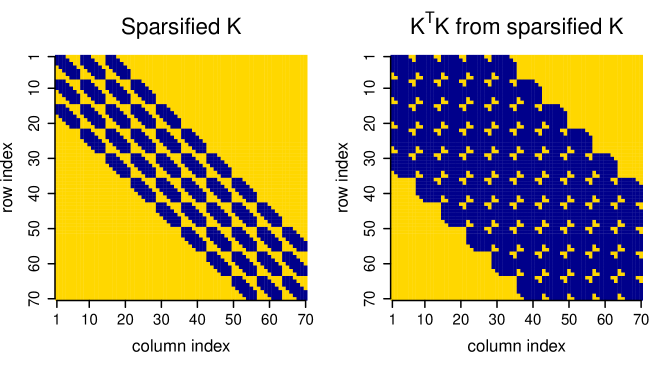
Figure 5: Representation of a sparse $\boldsymbol{K}$ matrix of size $70\times 70$ for an inverse problem over a pixel grid of size $7\times 10$ (left panel) and the corresponding $\boldsymbol{K}^{T}\boldsymbol{K}$ matrix (right panel). These matrices are obtained by using a truncation number $\ell=2$. Non-zero values are depicted in blue.

The suggested sparsification strategy has a physical interpretation. In the two-dimensional problems under examination each element of $\boldsymbol{Y}$ linearly depends on a subset of the elements of $\boldsymbol{X}$ through $\boldsymbol{K}$. If the elements of $\boldsymbol{K}$ are set to zero according to a truncation number $\ell$, then such subset is given by those elements of $\boldsymbol{X}$ that fall inside of a circle of diameter $2\ell+1$ around the element of $\boldsymbol{X}$ having one-to-one correspondence with the $\boldsymbol{Y}$ entry. Sparsifying the expression to be inverted in (27) means setting to zero some elements of the precision matrix $\boldsymbol{\Omega}_{q(\boldsymbol{x})}=\boldsymbol{\Sigma}_{q\left(\boldsymbol{x}\right)}^{-1}$, where $\boldsymbol{\Sigma}_{q\left(\boldsymbol{x}\right)}$ is the covariance matrix of the optimal approximating density function $q^{*}(\boldsymbol{x})$ in (9). Since $q^{*}(\boldsymbol{x})$ is a Multivariate Normal density function, $\big{(}\boldsymbol{\Omega}_{q(\boldsymbol{x})}\big{)}_{ij}=0$, for $i,j=1,\ldots,m$, if and only if $x_{i}$ and $x_{j}$ are conditionally independent given all the other elements of $\boldsymbol{x}$.

Note that differently from the algebraic results proposed for removal of $\boldsymbol{L}$, the sparsification applied to $\boldsymbol{K}$ comes from nullifying interactions between elements of $\boldsymbol{X}$ and $\boldsymbol{Y}$, and therefore it introduces another level of approximation to the variational fitting procedure.

4.2.1 Block-Banded Matrix Algebra

Asif and Moura (2005) propose two algorithms to invert block-banded matrices whose inverses are positive definite matrices: one resorting to Cholesky factors and an alternative implementation that avoids Cholesky factorizations. These algorithms require the inversion of smaller matrices having the size of the block-banded matrix sub-blocks. In the two-dimensional inverse problems under examination these sub-blocks have a banded structure. An approach for inverting banded matrices is described in Kiliç and Stanica (2013). These algebraic approaches for handling block-banded and banded matrices may allow for stable computation of variational algorithm steps involving sparse matrix inversions such as (23). However, the simplest way to perform efficient sparse matrix inversion and computations is to employ software for sparse matrix algebra. The functions contained in the R package spam (Furrer and Sain, 2010) allow efficient management of sparse matrices and implement matrix operations. This package can be used in combination with package spam64 (Gerber et al., 2017) to speed up such functions in 64 bit machines. Well established software is also available for lower-level languages such as the linear algebra libraries Armadillo and Eigen for C++ coding.

In general, matrices having banded or block-banded inverses are full matrices. Nonetheless, the inverse of a banded matrix may be referred to as band-dominated matrix (Bickel and Lindner, 2012), since the entries of its inverse exponentially decay with the distance from the main diagonal (Demko et al., 1984, Theorem 2.4). This property can be generalized to block-banded matrices and the inverse of a block-banded matrix can be approximated by a block-banded matrix with the same sparsity structure, i.e. with zero blocks off the main block band (Wijewardhana and Codreanu, 2016). The blocks outside the $\ell$-block band of a symmetric positive definite matrix having an $\ell$-block-banded inverse are called nonsignificant blocks and those in the $\ell$-block band are called significant blocks. Theorem 3 of Asif and Moura (2005) states that nonsignificant blocks can be obtained from the significant ones. Then, a possible way to further speed-up algebra involving these matrices and reduce memory usage is to impose a block-banded structure to the precision matrix $\boldsymbol{\Omega}_{q(\boldsymbol{x})}$ and approximate $\boldsymbol{\Sigma}_{q\left(\boldsymbol{x}\right)}$ with a block-banded matrix having the same structure of $\boldsymbol{\Omega}_{q(\boldsymbol{x})}$. In this case only the significant blocks of the covariance matrix $\boldsymbol{\Sigma}_{q\left(\boldsymbol{x}\right)}$, which solely depend on the significant blocks of $\boldsymbol{\Omega}_{q(\boldsymbol{x})}$, need to be computed.

5 Biomedical Data Study

This section demonstrates the use of variational inference for two-dimensional inverse problems motivated by a biomedical application. An illustration on a real dataset and on simulations that mimic the real data are provided.

We assess the performances of variational inference through comparison with MCMC and computation of accuracy. For a generic univariate parameter $\theta$, the approximation accuracy of a density $q(\theta)$ to a posterior density $p(\theta|\boldsymbol{y})$ is measured through

$$\mbox{accuracy}\equiv 100\left\{1-\frac{1}{2}\int_{-\infty}^{\infty}\big{|}q(\theta)-p(\theta|\boldsymbol{y})\big{|}d\theta\right\}\%,$$ (29)

so that $0\%\leq\mbox{accuracy}\leq 100\%$, with $100\%$ indicating perfect matching between the approximating and posterior density functions. We compute accuracy using Markov chain Monte Carlo as a benchmark. A standard Metropolis–Hastings algorithm (Metropolis et al., 1953; Hastings, 1970) is used to produce approximate samples from the posterior distribution. The Markov chains are started at feasible points in the parameter space and the retained samples are used to approximate the corresponding posterior density functions via kernel density estimation. Accuracy is then obtained from (29) with replacement of $p(\theta|\boldsymbol{y})$ by MCMC density estimates of the posterior density functions. Variational inference is performed removing the contrast matrix $\boldsymbol{L}$ through Lemmas 4–6 and sparsifying the kernel matrix $\boldsymbol{K}$ via truncation of interactions, as explained in Section 4, whereas our MCMC implementation does not make direct use of matrices $\boldsymbol{L}$ and $\boldsymbol{K}$. The simulation study is run on a personal computer with a 64 bit Windows 10 operating system, an Intel i7-7500U central processing unit at 2.7 gigahertz and 16 gigabytes of random access memory. Variational inference is fully performed in R, whereas MCMC is run in R with subroutines replacing $\boldsymbol{L}$ and $\boldsymbol{K}$ matrix operations implemented in C++.

5.1 Real Biomedical Data

We test the performance of our variational inference approach on a real biomedical application from the realm of tomographic data. Tomography aims to display cross-sections through human and animal bodies, or other solid objects, using data collected around the body.

The data, kindly provided by BioEmission Technology Solutions, Athens, Greece, were collected to illustrate a small animal imaging system, gamma-eye, which can be used in biotechnology and pre-clinical medical research (Georgiou et al., 2017). A technetium radioisotope (99m Tc-MIBI) was injected via the tail vein of a mouse and mainly absorbed by organs such as heart, liver and kidneys, and then excreted. In humans such techniques are used to monitor heart function and mice are often used in pre-clinical studies. A single plane gamma-camera image of an adult mouse was collected with the camera at a distance of 5mm from the nearest point of the mouse and 35mm from the support bed. The $29\times 58$, pixels of the data image are 1.7mm apart giving a field of view of about 5cm by 10cm. The mouse was anesthetized and so this corresponds to the “at rest” part of a human scan which would also involve a “stress test”. The total data recording time was 3 hours.

The objective is to reconstruct an image by removing blur from the observed scan of the mouse shown and denoted as $\boldsymbol{Y}$ in Figure 6. We adopt model (2) setting $\boldsymbol{y}=\mathop{\mbox{\rm vec}}(\boldsymbol{Y})$ and using a Gaussian kernel matrix $\boldsymbol{K}$ obtained through (6) with $\delta=0.7$. Hence, $\boldsymbol{y}$ and $\boldsymbol{x}$ are vectors of length equal to the number of pixels, 1,682, and $\boldsymbol{K}$ has size $1,682\times 1,682$. We set to zero the elements of $\boldsymbol{K}$ expressing interactions between locations that have 10 or more pixels between each other using $\ell=10$. The random walk Metropolis–Hastings algorithm is used to produce approximate samples from the posterior distribution by simulating a Markov chain with burn-in of 1000 followed by 100,000, then thinned by a factor of 20. Hyperparameters are set to values that give rise to diffuse priors. Specifically, $A_{\varepsilon}=A_{x}=10^{5}$. Estimates of $\boldsymbol{X}$ obtained via variational inference and MCMC are included in Figure 6. Here the term variational inference refers to both MFVB and VMP, as they both provide the same results by construction. The estimate of $\boldsymbol{X}$ obtained via variational inference corresponds to the inverse vectorization of $\boldsymbol{\mu}_{q(\boldsymbol{x})}$ from (9), whereas that of MCMC is given by the mean of the sampled chains. Figure 6 also displays approximate posterior density plots for a selection of six representative pixels. Five of the six selected pixels correspond to targeted organs of the mouse, namely thyroid, liver, kidneys and bladder, while the remaining pixel is located outside but near the mouse body. Overall variational approximations provide good image reconstruction and facilitate visualisation of the mouse body shape and organs. The posterior density approximations are also satisfactory in terms of accuracy, that is, area overlap between MCMC. As typical of variational approximations based on mean field restrictions, variational inference underestimates the variance of the approximate posterior densities.

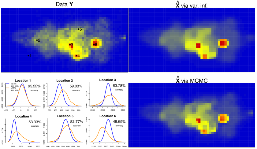
Figure 6: Analysis of the data provided by BioEmission Technology Solutions, Athens, Greece, performed by fitting model (2) via variational inference and MCMC. The panel on the upper-left side displays the observed data $\boldsymbol{Y}$. The two panels on the left-hand side show, from top to bottom, the reconstruction $\widehat{\boldsymbol{X}}$ of $\boldsymbol{X}$ obtained via variational inference and MCMC. The plots on the lower-left side show the approximate marginal posterior densities produces through variational inference (blue lines) and MCMC (orange lines) for a selection of pixels.

5.2 Simulated Biomedical Data

We employ the real biomedical data image processed through MCMC, the one corresponding to the lower-right panel of Figure 6, to simulate datasets and study the performance of variational inference in comparison with MCMC. In this simulation study we also keep track of computational times and calculate percentages of coverage. For a given parameter, the percentage of coverage corresponds to the proportion of simulations where the true parameter falls inside its 95% credible interval obtained through variational inference.

Let $\widehat{\boldsymbol{X}}_{\tiny\mbox{MCMC}}$ be the inverse vectorization of the estimate of $\boldsymbol{x}$ obtained as the sample mean of the corresponding MCMC chains. We simulate data through:

$$\boldsymbol{y}=\boldsymbol{K}\mathop{\mbox{\rm vec}}(\widehat{\boldsymbol{X}}_{\tiny\mbox{MCMC}})+\boldsymbol{\varepsilon},\quad\boldsymbol{\varepsilon}\sim N(\boldsymbol{0},\sigma^{2}_{\varepsilon}\boldsymbol{I}),$$

with $\sigma_{\varepsilon}=50$ and $\boldsymbol{K}$ generated according to (6), using $\delta$ values from the set $(0.7,0.8,0.9)$ and without truncating interactions ($\ell=\infty$). The example plots provided in the supplementary information show how the blur increases for higher $\delta$. For each $\delta$ value we generate 100 datasets and fit model (2) via both MFVB and MCMC. For fitting we apply the same $\boldsymbol{K}$ matrix used to generate the datasets, i.e. without truncation of interactions, but also fit the model again setting to zero the elements of $\boldsymbol{K}$ associated with pairs of observations whose distance exceeds a truncation value $\ell=5$. The MFVB algorithm is stopped when the relative difference of estimates of $\boldsymbol{X}$ goes below $10^{-2}$ between two iterations. We generate Markov chains of length 6,000 and retain 5,000 of them after discarding 1,000 warm-up samples.

Table 3 summarizes the results of the simulation study including: accuracy of the variational inference estimates of $\boldsymbol{X}$ versus MCMC; variational inference percentage of coverage for $\boldsymbol{X}$, i.e. the number of times the entries of $\widehat{\boldsymbol{X}}_{\tiny\mbox{MCMC}}$ falls inside their 95% variational inference credible intervals; variational inference and MCMC computational times. Average and standard deviations (in brackets) of each indicator are displayed for each combination of $\delta$ and $\ell$ values.

For each pixel of each simulated dataset we compute the accuracy of the variational approximation using (29) and then average over the 100 replicates. We then calculate average and standard deviation over all the entries of $\boldsymbol{X}$ and display these in Table 3. We repeat the same procedure for measuring the percentage of coverage performances. The mean accuracy values range between 88.07 and 87.10, whereas the mean percentages of coverage are between 95.09 and 92.75 and therefore close to the nominal 95% level. Both accuracy and coverage performances slightly degrade for higher values of $\delta$ and blur.

The variational inference and MCMC computational times are displayed in minutes and show that variational inference is around 100 times faster for the $\delta=0.7$ setting. Imposing a truncation $\ell=5$ to $\boldsymbol{K}$ reduces MCMC computational times. The time performances of variational inference are not particularly affected by truncation as the R package spam efficiently manages the algorithm updates involving $\boldsymbol{K}$ in both cases with and without truncation. Once again, variational inference has been fully performed in R, while the main MCMC function has been implemented in R and uses C++ subroutines that replace the $\boldsymbol{K}$ and $\boldsymbol{L}$ matrix operations. Therefore, further computational advantages may be achieved implementing variational inference in C++.

		$\ell=\infty$ (no truncation)	$\ell=5$
$\delta=0.7$	Var. inf. vs MCMC accuracy for $\boldsymbol{X}$	88.07 (4.23)	88.04 (4.23)
	Var. inf. percentage of coverage for $\boldsymbol{X}$	95.09 (16.36)	95.09 (16.36)
	Var. inf. comp. time (minutes)	0.85 (0.24)	0.84 (0.24)
	MCMC comp. time (minutes)	87.67 (0.29)	81.61 (0.39)
$\delta=0.8$	Var. inf. vs MCMC accuracy for $\boldsymbol{X}$	87.54 (5.17)	87.55 (5.20)
	Var. inf. percentage of coverage for $\boldsymbol{X}$	94.01 (19.12)	94.01 (19.12)
	Var. inf. comp. time (minutes)	1.20 (0.28)	1.19 (0.28)
	MCMC comp. time (minutes)	88.08 (0.57)	82.12 (0.58)
$\delta=0.9$	Var. inf. vs MCMC accuracy for $\boldsymbol{X}$	87.10 (5.58)	87.12 (5.65)
	Var. inf. percentage of coverage for $\boldsymbol{X}$	92.75 (22.02)	92.75 (22.02)
	Var. inf. comp. time (minutes)	1.43 (0.43)	1.43 (0.43)
	MCMC comp. time (minutes)	88.64 (0.30)	81.70 (0.44)

Table 3: Results of the simulation study based on 100 replicates per $\delta$ value generated using the kernel matrix $\boldsymbol{K}$ defined in (6) without truncation. Fitting is performed via variational inference and MCMC using the same $\boldsymbol{K}$ matrix employed to generate the data (no truncation) and also imposing a truncation threshold $\ell=5$ to the interactions expressed by $\boldsymbol{K}$. Higher $\delta$ values correspond to more blur. The smaller $\ell$, the sparser the $\boldsymbol{K}$ matrix used to fit the model is.

6 Illustration for Archaeological Data

We here show how the message passing on factor graph fragments paradigm can be used to move from an inverse problem model analysis to another without deriving a variational inference algorithm from scratch. This is illustrated through data from archaeological magnetometry. In archaeology it is often required to investigate a potential site via geophysical remote sensing methods before any physical excavation is commenced. The model we consider includes a Skew Normal distribution for the response vector and a Horseshoe penalization in replacement to the Normal response and Laplace penalization of model (2).

The data were collected from a mid Iron Age farmstead known as ‘The Park’ through an archaeological exploration that took place in 1994 at Guiting Power in Gloucestershire, United Kingdom. After data collection, part of the area was also excavated and archaeologists drew an impression of the remains that were brought to light.

The archaeological site was partitioned into a grid of 10m$\times$10m squares with the survey axes aligned in the directions of magnetic north and east. A fluxgate gradiometer FM18 with 0.1nT sensitivity was used to collect the data at 0.5m intervals. For each survey square, the gradiometer output was an array of $20\times 20$ magnetic anomaly readings corresponding to the difference between the signals detected by the lower and upper sensors. The gradiometer lower sensor was held at 0.2m above the surface of the site and the upper sensor was fixed a further 0.5m higher. The Earth’s magnetic field is detected by both sensors, whereas the magnetic field from the buried feature is mostly detected by the lower sensor. Therefore the difference between the two sensors’ readings provides the magnetic anomaly due to the hidden feature, together with small random noise components. The random noise may be due to systematic causes such as machine-rounding errors, or non-systematic factors such as disturbance by small stones in the soil or interference from local magnetic sources (Scollar, 1970).

We model the hidden surface through a single layer of rectangular prisms at a fixed burial depth. The scope is to estimate the prisms’ magnetic susceptibility in order to separate the constituent epochs of the site. The subsurface layer is assumed to be fixed at a burial depth of 0.3m, given that the topsoil across the excavated region of Guiting Power was found to be between 0.25 and 0.3m deep. According to the single layer subsurface model, each prism in the layer has the same constant extent, which we set to 0.5m. Although the vertical extent of each of the excavated features vary from 0.45m to 1.6m, the chosen value of prism vertical extent increases the chances of distinguishing low-susceptibility features.

All this information is relevant to design an appropriate kernel matrix $\boldsymbol{K}$ suitable for inverse problems concerning archaeological data. The assumptions and steps to derive the kernel matrix are summarized in the supplementary information. As affirmed in Aykroyd et al. (2001), these assumptions provide a realistic basis for modeling the data but can be quite restrictive. The recorded magnetic anomaly may include both positive and negative values, generate shifts in the apparent location of features, be asymmetric in shape and vary across different sampling regions. For this reason we model the outcome variable $\boldsymbol{y}$, i.e. the anomaly detected by the gradiometer, through a Skew Normal distribution and impose a Horseshoe penalization to the difference between hidden susceptibility values $\boldsymbol{x}_{\Delta}$. The Horseshoe prior shrinks the small signals and enhances the big ones, highlighting the contrast between buried features and plain soil.

The model we fit is the following:

$$\begin{array}[]{c}y_{i}|\boldsymbol{x},\sigma^{2}_{\varepsilon},\lambda,c_{i}\stackrel{{\scriptstyle{\tiny\mbox{ind.}}}}{{\sim}}N\left(\left(\boldsymbol{K}\boldsymbol{x}\right)_{i}+\frac{\sigma^{2}_{\varepsilon}\lambda|c_{i}|}{\sqrt{1+\lambda^{2}}},\frac{\sigma^{2}_{\varepsilon}}{1+\lambda^{2}}\right),\quad c_{i}\stackrel{{\scriptstyle{\tiny\mbox{ind.}}}}{{\sim}}N(0,1),\quad i=1,\ldots,m,\\[4.30554pt] (\boldsymbol{x}_{\Delta})_{j}|b_{j},\sigma^{2}_{x}\stackrel{{\scriptstyle{\tiny\mbox{ind.}}}}{{\sim}}N\left(0,\sigma^{2}_{x}/b_{j}\right),\quad b_{j}\stackrel{{\scriptstyle{\tiny\mbox{ind.}}}}{{\sim}}\pi^{-1}b_{j}^{-1/2}\left(1+b_{j}\right)^{-1},\quad j=1,\ldots,d,\\[4.30554pt] \sigma^{2}_{\varepsilon}\sim\mbox{Inverse-}\chi^{2}\left(A_{\varepsilon},B_{\varepsilon}\right),\quad\lambda\sim N\left(0,S^{2}_{\lambda}\right),\\[4.30554pt] \sigma^{2}_{x}|a_{x}\sim\mbox{Inverse-$\chi^{2}$}\left(1,1/a_{x}\right),\quad a_{x}\sim\mbox{Inverse-$\chi^{2}$}\left(1,1/A^{2}_{x}\right).\end{array}$$ (30)

The first line of this model gives rise to a Skew Normal likelihood and is equivalent to

$$y_{i}|\boldsymbol{x},\sigma^{2}_{\varepsilon},\lambda\stackrel{{\scriptstyle{\tiny\mbox{ind.}}}}{{\sim}}\mbox{Skew-Normal}\left(\left(\boldsymbol{K}\boldsymbol{x}\right)_{i},\sigma^{2}_{\varepsilon},\lambda\right).$$

Here the density function of a random variable $z$ having a $\mbox{Skew-Normal}\left(\mu,\sigma^{2},\lambda\right)$ distribution is $p(z)=(2/\sigma)\phi\{(z-\mu)/\sigma\}\}\Phi\{\lambda(z-\mu)/\sigma\}$, with scale parameter $\sigma>0$, skewness parameter $\lambda$, and $\phi$ and $\Phi$ denoting the Standard Normal density and cumulative distribution functions. The second line of (30) specifies a Horseshoe penalization on the $(\boldsymbol{x}_{\Delta})_{j}$’s, as indicated by Table 1. The priors at line three give rise to conjugate message passing updates for the stochastic nodes of $\sigma_{\varepsilon}$ and $\lambda$. As in model (2), $\sigma_{x}$ is assigned a Half-Cauchy$\left(A_{x}\right)$ prior through the auxiliary variable $a_{x}$.

The joint density function of model (30) is given by

$$\begin{split}p\left(\boldsymbol{y},\boldsymbol{x},\boldsymbol{c},\boldsymbol{b},\sigma^{2}_{\varepsilon},\lambda,\sigma_{x}^{2},a_{x}\right)&=p\left(\boldsymbol{y}|\boldsymbol{x},\boldsymbol{c},\sigma^{2}_{\varepsilon},\lambda\right)p\left(\boldsymbol{x}|\boldsymbol{b},\sigma^{2}_{x}\right)p\left(\boldsymbol{c}\right)p\left(\boldsymbol{b}\right)\\ &\quad\times p\left(\sigma^{2}_{\varepsilon}\right)p\left(\lambda\right)p\left(\sigma^{2}_{x}|a_{x}\right)p\left(a_{x}\right).\end{split}$$ (31)

Steps similar to those presented for the base model can be used to implement VMP for the model with Skew Normal responses and Horseshoe prior. The starting point is again the choice of a factorization for the approximating $q$-densities. We impose the following mean field approximation to the joint posterior:

$$p\left(\boldsymbol{x},\boldsymbol{c},\boldsymbol{b},\sigma^{2}_{\varepsilon},\lambda,\sigma_{x}^{2},a_{x}|\boldsymbol{y}\right)\approx q\left(\boldsymbol{x}\right)q\left(\sigma^{2}_{\varepsilon}\right)q\left(\lambda\right)q\left(\sigma^{2}_{x}\right)q\left(a_{x}\right)\prod_{i=1}^{m}q_{i}\left(c_{i}\right)\prod_{j=1}^{d}q_{j}\left(b_{j}\right).$$ (32)

The right-hand sides of (31) and (32) give rise to the factor graph representation displayed as Figure 7.

Figure 7: Factor graph representation of the Skew Normal response model with Horseshoe penalization in (30), where the square nodes correspond to the density functions, or factors, on the right-hand side of (31). The circular nodes correspond to stochastic nodes of the $q$-density factorization in (32). Numbers are used to show the distinction between fragments, whereas colors identify different fragments types.

In this factor graph, four of the seven fragments arising from the base model (2), those numbered 1–3, are preserved. Fragment 4 is now the Skew Normal likelihood fragment studied in Section 3.4 of McLean and Wand (2019). The message passed from this fragment to $\sigma^{2}_{\varepsilon}$ takes the form

$$m_{p(\boldsymbol{y}|\boldsymbol{x},\sigma^{2}_{\varepsilon},\lambda,\boldsymbol{c})\rightarrow\sigma_{\varepsilon}^{2}}(\sigma_{\varepsilon}^{2})=\exp\left\{\left[\begin{array}[]{c}\log(\sigma_{\varepsilon}^{2})\\[4.30554pt] 1/\sigma_{\varepsilon}\\[4.30554pt] 1/\sigma_{\varepsilon}^{2}\end{array}\right]^{T}\mbox{\large$\boldsymbol{\eta}$}_{p(\boldsymbol{y}|\boldsymbol{x},\sigma^{2}_{\varepsilon},\lambda,\boldsymbol{c})\rightarrow\sigma_{\varepsilon}^{2}}\right\}$$ (33)

and is proportional to an Inverse Square Root Nadarajah density function, whereas the message to $\lambda$ is

$$m_{p(\boldsymbol{y}|\boldsymbol{x},\sigma^{2}_{\varepsilon},\lambda,\boldsymbol{c})\rightarrow\lambda}(\lambda)=\exp\left\{\left[\begin{array}[]{c}\log(1+\lambda^{2})\\[4.30554pt] \lambda^{2}\\[4.30554pt] \lambda\sqrt{1+\lambda^{2}}\end{array}\right]^{T}\mbox{\large$\boldsymbol{\eta}$}_{p(\boldsymbol{y}|\boldsymbol{x},\sigma^{2}_{\varepsilon},\lambda,\boldsymbol{c})\rightarrow\lambda}\right\}$$ (34)

and is part of the Sea Sponge family. These two families of distributions are defined in Sections S.2.3 and S.2.5 of the supplementary material of McLean and Wand (2019). Priors on $\sigma_{\varepsilon}^{2}$ and $\lambda$ that are conjugate to these messages must have the form

$$m_{p(\sigma_{\varepsilon}^{2})\rightarrow\sigma_{\varepsilon}^{2}}(\sigma_{\varepsilon}^{2})=\exp\left\{\left[\begin{array}[]{c}\log(\sigma_{\varepsilon}^{2})\\[4.30554pt] 1/\sigma_{\varepsilon}\\[4.30554pt] 1/\sigma_{\varepsilon}^{2}\end{array}\right]^{T}\mbox{\large$\boldsymbol{\eta}$}_{p(\sigma_{\varepsilon}^{2})\rightarrow\sigma_{\varepsilon}^{2}}\right\}$$ (38)

and $$m_{p(\lambda)\rightarrow\lambda}(\lambda)=\exp\left\{\left[\begin{array}[]{c}\log(1+\lambda^{2})\\[4.30554pt] \lambda^{2}\\[4.30554pt] \lambda\sqrt{1+\lambda^{2}}\end{array}\right]^{T}\mbox{\large$\boldsymbol{\eta}$}_{p(\lambda)\rightarrow\lambda}\right\},$$ (42)

for some $3\times 1$ vectors $\mbox{\large$\boldsymbol{\eta}$}_{p(\sigma_{\varepsilon}^{2})\rightarrow\sigma_{\varepsilon}^{2}}$ and $\mbox{\large$\boldsymbol{\eta}$}_{p(\lambda)\rightarrow\lambda}$. Priors $\sigma^{2}_{\varepsilon}\sim\mbox{Inverse-}\chi^{2}\left(A_{\varepsilon},B_{\varepsilon}\right)$ and $\lambda\sim N\left(0,S^{2}_{\lambda}\right)$ of model (30) are respectively conjugate to (33) and (34), since for this choice of priors the messages $m_{p(\sigma_{\varepsilon}^{2})}(\sigma_{\varepsilon}^{2})$ and $m_{p(\lambda)\rightarrow\lambda}(\lambda)$ can be written as (38) and (42) with

$$\mbox{\large$\boldsymbol{\eta}$}_{p(\sigma_{\varepsilon}^{2})\rightarrow\sigma_{\varepsilon}^{2}}=[-(A_{\varepsilon}/2)-1\,\,\,\,0\,\,\,-B_{\varepsilon}/2]^{T}\,\,\mbox{and}\,\,\mbox{\large$\boldsymbol{\eta}$}_{p(\lambda)\rightarrow\lambda}=[0\,\,\,-1/(2S^{2}_{\lambda})\,\,\,\,0]^{T}.$$

We impose diffuse priors using $A_{\varepsilon}=B_{\varepsilon}=10^{-2}$ and $S_{\lambda}=10^{5}$.

Full implementation of VMP is based on iteratively updating, for each factor graph fragment depicted in Figure 7: (i) the parameter vectors of messages passed from the fragment’s neighboring stochastic nodes to the fragment’s factors; (ii) the parameter vectors of the messages passed from the fragment’s factors to their neighboring stochastic nodes. The first step is very simple and entails application of (7) of Wand (2017). The factor to stochastic node updates of the second step can be performed through various VMP procedures:

• Fragment 1 is an Inverse G-Wishart prior fragment and the factor to stochastic node parameter vector updates can be performed using Algorithm 1 of Maestrini and Wand (2021) with inputs $G_{\Theta}=G_{\tiny\mbox{full}}$, $\xi_{\Theta}=1$ and $\boldsymbol{\Lambda}_{\Theta}=(A_{x}^{2})^{-1}$.

• Fragment 2 is an iterated Inverse G-Wishart prior fragment and the factor to stochastic node parameter vector updates can be performed using Algorithm 2 of Maestrini and Wand (2021) with inputs $G=G_{\tiny\mbox{full}}$, $\xi=1$ and $G_{\boldsymbol{A}\rightarrow p(\boldsymbol{\Sigma}|\boldsymbol{A})}=G_{\tiny\mbox{diag}}$.

• The factor to stochastic node parameter vector updates of fragment 3 can be performed through Algorithm 2.

• Fragment 4 is the Skew Normal likelihood fragment and the factor to stochastic node parameter vector updates can be performed using Algorithm 4 of McLean and Wand (2019) with $\boldsymbol{y}$ and $\boldsymbol{K}$ as data inputs.

• Fragment 5 corresponds to the imposition of an Inverse Square Root Nadarajah prior distribution on the variance parameter $\sigma^{2}_{\varepsilon}$. The output of VMP applied to this fragment is the natural parameter vector of the prior density function, that is, $\mbox{\large$\boldsymbol{\eta}$}_{p(\sigma_{\varepsilon}^{2})\rightarrow\sigma_{\varepsilon}^{2}}$ from (38).

• Fragment 6 corresponds to the imposition of a Sea Sponge prior distribution on the skewness parameter $\lambda$. The output of VMP applied to this fragment is the natural parameter vector of the prior density function, that is, $\mbox{\large$\boldsymbol{\eta}$}_{p(\lambda)\rightarrow\lambda}$ from (42).

We restrict our attention to the portion of the archaeological dataset corresponding to the excavated area, which enables a qualitative performance assessment of our fitting method. Figure 8 displays the data under examination ($\boldsymbol{Y}$) together with the results of the application of VMP to model (30) and the impression drawn by archaeologists. The data were handled in a disjoint way by separating the two rectangular areas corresponding to indices J and K of the archaeologists’ impression. It is standard practice to examine grids as soon as they are collected and this division of the surveyed area allows to partition the data into two full matrices $\boldsymbol{Y}_{J}$ for area J and $\boldsymbol{Y}_{K}$ for area K of size $30\times 20$ and $40\times 20$, respectively. Model (30) can be used setting $\boldsymbol{y}=\mathop{\mbox{\rm vec}}(\boldsymbol{Y}_{J})$ or $\boldsymbol{y}=\mathop{\mbox{\rm vec}}(\boldsymbol{Y}_{K})$ and the reconstruction $\widehat{\boldsymbol{X}}$ is simply obtained as the inverse vectorization of the VMP estimate of $\boldsymbol{x}$. We employ the mean of the optimal approximating density $q^{*}(\boldsymbol{x})$, which is a $N\big{(}\boldsymbol{\mu}_{q\left(\boldsymbol{x}\right)},\boldsymbol{\Sigma}_{q\left(\boldsymbol{x}\right)}\big{)}$ density function, to estimate $\boldsymbol{x}$. Expressions for $q^{*}(\boldsymbol{x})$ and the other $q$-densities of interest are provided in the supplementary information.

If compared to the original dataset, the VMP reconstruction of Figure 8 shows greater contrast between background and features, and some weak features are more evident in the posterior mean reconstruction. Despite the data being treated in a disjoint way, discontinuity in the estimate of $\boldsymbol{X}$ between areas J and K is not very apparent. Careful inspection of the reconstruction shows the locations of some reconstructed features are shifted if compared to their apparent position in the original survey data image. This is important information, considering that each pixel corresponds to a square area of 0.5m side and that archaeological excavations require intensive manual work. The approximate posterior densities of $\lambda$ seem to indicate that the data from area J is symmetric, whereas that from area K is positively skewed.

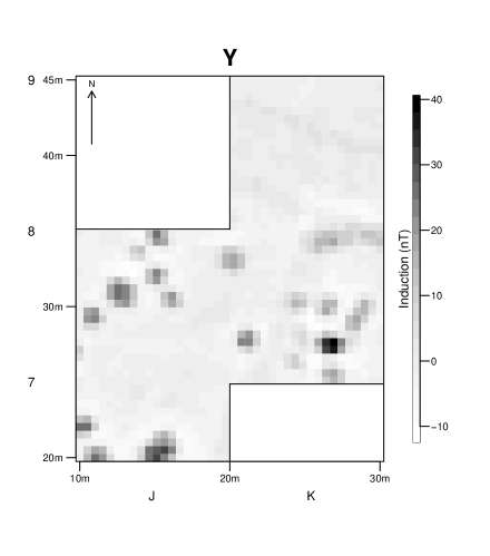
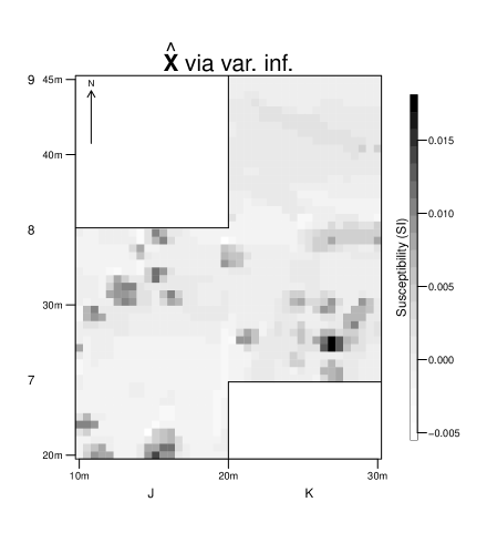
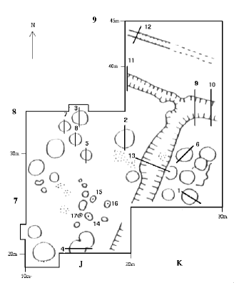
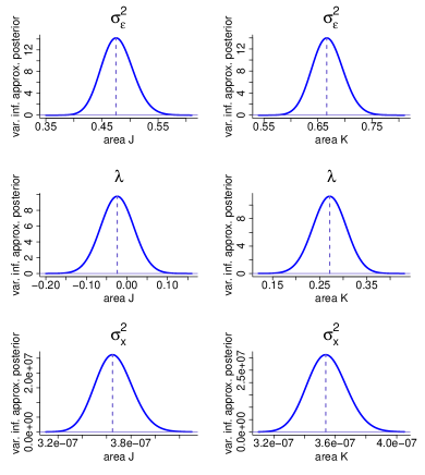
Figure 8: Results of the archaeological data study conducted via model (30) and variational inference. The top-left image displays the archaeological dataset denoted by $\boldsymbol{Y}$. Its variational inference reconstruction, denoted by $\widehat{\boldsymbol{X}}$, is shown in the top-right image, whereas the bottom-left image corresponds to the archaeologist’s impression of the 1994 excavation of ‘The Park’. The plots in the bottom-right side show the variational approximate marginal posterior densities of the Skew Normal variance and skewness parameters for areas J and K of the archaeological site.

          

7 Discussion

We have laid down the infrastructure for performing variational approximate inference on applications that can be studied through statistical inverse problems models. Our variational algorithms allow fast approximate fitting for these models, with satisfactory accuracy compared with standard MCMC.

The run-time of MCMC estimation for inverse problems is usually excessive on a standard personal computer. This means that parameter tuning, model diagnostics and sensitivity analyses are rarely performed. The use of variational inference methods, which are quick by comparison, means that multiple parameter settings and multiple models can be considered in a reasonable length of time. This opens-up the possibility of model diagnostics, such as influence and leverage, to become a routine part of applied inverse problems solution. Further, there is a subjective element, as always, to the choice of model components and in particular the hierarchical prior components. It would be a great advance for applications areas, such as medicine and archaeology, if rogue measurements could be identified and their influence on estimation could be quantified. Also, if any arbitrary parts could be shown to have insignificant effect on results, this would lead to far greater confidence and hence a wider acceptability of advanced statistical modelling approaches.

Hence, the implications of our work are not limited to the numerical results presented, but we provide a framework for other researchers to develop a richer set of model exploration methods for inverse problems. The flexibility of our approach is such that non-Normal likelihood distributions and other penalizations can be incorporated at will. Furthermore, this research sets the basis for several future directions to explore such as the study of settings with more than two dimensions, number of observations not matching that of data recording locations or more complex neighbor dependence structures.

References

Agrawal, S., Kim, H., Sanz-Alonso, D. and Strang, A. (2021). A Variational Inference Approach to Inverse Problems with Gamma Hyperpriors. arXiv preprint arXiv:2111.13329.

Allum, G.T., Aykroyd, R.G. and Haigh, J.G.B. (1999). Empirical Bayes estimation for archaeological stratigraphy. Journal of the Royal Statistical Society: Series C (Applied Statistics), 48, 1–14.

Asif, A. and Moura, J.M.F. (2005). Block matrices with L-block-banded inverse: inversion algorithms. IEEE Transactions on Signal Processing, 53, 630–642.

Aykroyd, R.G., Haigh, J.G.B. and Allum., G.T. (2001). Bayesian methods applied to survey data from archeological magnetometry. Journal of the American Statistical Association, 96, 64–76.

Armagan, A., Dunson, D.B. and Lee, J. (2013). Generalized double Pareto shrinkage. Statistica Sinica, 23, 119–143.

Arridge, S.R., Ito, K., Jin, B. and Zhang, C. (2018). Variational Gaussian approximation for Poisson data. Inverse Problems, 34, 1–29.

Bickel, P. and Lindner, M. (2012). Approximating the inverse of banded matrices by banded matrices with applications to probability and statistics. Theory of Probability & Its Applications, 56, 1–20.

Carvalho, C.M., Polson, N.G. and Scott, J.G. (2010). The horseshoe estimator for sparse signals. Biometrika, 97, 465–480.

Demko, S., Moss, W.F. and Smith, P.W. (1984). Decay rates for inverses of band matrices. Mathematics of Computation, 43, 491–499.

Donoho, D.L. and Johnstone, I.M. (1994). Ideal spatial adaptation by wavelet shrinkage. Biometrika, 81, 425–455.

Furrer, R. and Sain, S.R. (2010). spam: A sparse matrix R package with emphasis on MCMC methods for Gaussian Markov random fields. Journal of Statistical Software, 36, 1–25. http://www.jstatsoft.org/v36/i10/.

Gehre, M. and Jin, B. (2014). Expectation propagation for nonlinear inverse problems – with an application to impedance tomography. Journal of Computational Physics, 259, 513–535.

Georgiou, M., Fysikopoulos, E., Mikropoulos, K., Fragogeorgi, E. and Loudos, G. (2017). Characterization of ”$\gamma$-eye”: a low-cost benchtop mouse-sized gamma camera for dynamic and static imaging studies. Molecular Imaging and Biology, 19, 398–407.

Gerber, F., Mösinger, K. and Furrer, R. (2017). Extending R packages to support 64-bit compiled code: An illustration with spam64 and GIMMS NDVI3g data. Computer & Geoscience, 104, 109–119. https://doi.org/10.1016/j.cageo.2016.11.015.

Griffin, J.E. and Brown, P.J. (2011). Bayesian hyper-lassos with nonconvex penalization. Australian and New Zealand Journal of Statistics, 53, 423–442.

Guha, N., Wu, X., Efendiev, Y., Jin, B. and Mallick, B.K. (2015). A variational Bayesian approach to inverse problems with skew-t error distributions. Journal of Computational Physics, 301, 377–393.

Hadamard, J. (1902). Sur les problèmes aux dérivées partielles et leur signification physique. Princeton University Bulletin, 49–52.

Hastings, W.K. (1970). Monte Carlo sampling methods using Markov chains, and their applications. Biometrika, 57, 97–109.

Kiebel, S., Daunizeau, J., Phillips, C. and Friston, K. (2008). Variational Bayesian Inversion of the Equivalent Current Dipole Model in EEG/MEG. NeuroImage, 39, 728–741.

Kiliç, E. and Stanica, P. (2013). The inverse of banded matrices. Journal of Computational and Applied Mathematics, 237, 126–135.

Maestrini, L. and Wand, M.P. (2018). Variational message passing for Skew $t$ regression. Stat, 7, 1–11.

Maestrini, L. and Wand, M.P. (2021). The inverse G-Wishart distribution and variational message passing. Australian and New Zealand Journal of Statistics, 63, 517–541.

McGrory, C.A., Titterington, D.M., Reeves, R. and Pettitt, A.N. (2009). Variational Bayes for estimating the parameters of a hidden Potts model. Statistics and Computing, 19, 329–340.

McLean, M.W. and Wand, M.P. (2019). Variational message passing for elaborate response regression models. Bayesian Analysis, 14, 371–398.

Metropolis, N., Rosenbluth, A., Rosenbluth, M., Teller, A. and Teller, E. (1953). Equations of state calculations by fast computing machines. Journal of Chemical Physics, 21, 1087–1091.

Nason, G. (2008). Wavelet Methods in Statistics with R. New York: Springer Science & Business Media.

Nason, G. (2013). wavethresh: Wavelets statistics and transforms. R package version 4.6.

Nathoo, F.S., Babul, A., Moiseev, A., Virji-Babul, N. and Beg, M.F. (2014). A variational Bayes spatiotemporal model for electronmagnetic brain mapping. Biometrics, 70, 132–143.

Neville, S.E., Ormerod, J.T. and Wand, M.P. (2014). Mean field variational Bayes for continuous sparse signal shrinkage: pitfalls and remedies. Electonic Journal of Statistics, 8, 1113–1151.

Nolan, T.H. and Wand, M.P. (2017). Accurate logistic variational message passing: algebraic and numerical details. Stat, 6, 102–112.

Ormerod, J.T., You, C. and Müller, S. (2017). A variational Bayes approach to variable selection. Electronic Journal of Statistics, 11, 3549–3594.

Park, T. and Casella, G. (2008). The Bayesian lasso. Journal of the American Statistical Association, 103, 681–686.

Povala, J., Kazlauskaite, I., Febrianto, E., Cirak, F. and Girolami, M. (2022). Variational Bayesian approximation of inverse problems using sparse precision matrices. Computer Methods in Applied Mechanics and Engineering, 393, 1–31.

R Core Team (2021). R: A language and environment for statistical computing. R Foundation for Statistical Computing, Vienna, Austria. https://www.R-project.org/.

Sato, M., Yoshioka, T., Kajihara, S., Toyama, K., Goda, N., Doya, K. and Kawato, M. (2004). Hierarchical Bayesian estimation for MEG inverse problem. NeuroImage, 23, 806–826.

Scollar, I. (1970). Fourier transformations for the evaluation of magnetic maps. Prospezioni Archeologiche, 5, 9–41.

Tonolini, F., Radford, J., Turpin, A., Faccio, D. and Murray-Smith, R. (2020). Variational inference for computational imaging inverse problems. Journal of Machine Learning Research, 21, 1–46.

Tung, D.T., Tran, M.N. and Cuong, T.M. (2019). Bayesian adaptive lasso with variational Bayes for variable selection in high-dimensional generalized linear mixed models. Communications in Statistics-Simulation and Computation, 48, 530–543.

Wand, M.P. (2017). Fast approximate inference for arbitrarily large semiparametric regression models via message passing (with discussion). Journal of the American Statistical Association, 112, 137–168.

Wand, M.P., Ormerod, J.T., Padoan, S.A. and Frühwirth, R. (2011). Mean field variational Bayes for elaborate distributions. Bayesian Analysis, 6, 847–900.

Wijewardhana, U.L. and Codreanu, M. (2016). A Bayesian approach for online recovery of streaming signals from compressive measurements. IEEE Transactions on Signal Processing, 65, 184–199.

Wipf, D. and Nagarajan, S. (2009). A unified Bayesian framework for MEG/EEG source imaging. NeuroImage, 44, 947–966.

Zhang, C., Arridge, S.R. and Jin, B. (2019). Expectation propagation for Poisson data. Inverse Problems, 35, 1–27.

Supplement for:

A Variational Inference Framework for Inverse Problems

By L. Maestrini¹, R.G. Aykroyd² and M.P. Wand³

¹The Australian National University, ²University of Leeds and ³University of Technology Sydney

S.1 Algorithm Derivations

This section provides full justification of Algorithms 1 and 2.

S.1.1 Derivation of Algorithm 1

The optimal approximating densities satisfy (8) of Wand et al. (2011). The full conditional density functions of each hidden node in the directed acyclic graph in Figure 3 allow to derive expressions for the optimal approximating densities.

First,

$$p\left(\boldsymbol{x}|\mbox{rest}\right) \propto p\left(\boldsymbol{y}|\boldsymbol{x},\sigma^{2}_{\varepsilon}\right)p\left(\boldsymbol{x}|\boldsymbol{b},\sigma^{2}_{x}\right)$$

$$\propto\exp\left[-\frac{1}{2}\left\{\boldsymbol{x}^{T}\boldsymbol{L}^{T}\left(\frac{1}{\sigma^{2}_{\varepsilon}}\boldsymbol{K}^{T}\boldsymbol{K}+\frac{1}{\sigma^{2}_{x}}\mathop{\mbox{\rm diag}}\left(\boldsymbol{b}\right)\right)\boldsymbol{L}\boldsymbol{x}-\frac{2}{\sigma^{2}_{\varepsilon}}\boldsymbol{x}^{T}\boldsymbol{K}^{T}\boldsymbol{y}\right\}\right],$$

that is,

$$\boldsymbol{x}|\mbox{rest}\sim N\left(\left(\frac{1}{\sigma^{2}_{\varepsilon}}\boldsymbol{K}^{T}\boldsymbol{K}+\frac{1}{\sigma^{2}_{x}}\boldsymbol{L}^{T}\mathop{\mbox{\rm diag}}\left(\boldsymbol{b}\right)\boldsymbol{L}\right)^{-1}\frac{1}{\sigma^{2}_{\varepsilon}}\boldsymbol{K}^{T}\boldsymbol{y},\left(\frac{1}{\sigma^{2}_{\varepsilon}}\boldsymbol{K}^{T}\boldsymbol{K}+\frac{1}{\sigma^{2}_{x}}\boldsymbol{L}^{T}\mathop{\mbox{\rm diag}}\left(b\right)\boldsymbol{L}\right)^{-1}\right).$$

Hence $q^{*}(\boldsymbol{x})$ is $N\big{(}\boldsymbol{\mu}_{q\left(\boldsymbol{x}\right)},\boldsymbol{\Sigma}_{q\left(\boldsymbol{x}\right)}\big{)}$ with

$$\boldsymbol{\Sigma}_{q\left(\boldsymbol{x}\right)}\equiv\left(\mu_{q(1/\sigma^{2}_{\varepsilon})}\boldsymbol{K}^{T}\boldsymbol{K}+\mu_{q(1/\sigma^{2}_{x})}\boldsymbol{L}^{T}\mathop{\mbox{\rm diag}}(\mu_{q(\boldsymbol{b})})\boldsymbol{L}\right)^{-1}\,\,\,\mbox{and}\,\,\,\boldsymbol{\mu}_{q\left(\boldsymbol{x}\right)}\equiv\mu_{q(1/\sigma_{\varepsilon}^{2})}\boldsymbol{\Sigma}_{q\left(\boldsymbol{x}\right)}\boldsymbol{K}^{T}\boldsymbol{y}.$$

Given that

$$p\left(\boldsymbol{b}\right)\propto\prod_{j=1}^{d}b_{j}^{-2}\exp\left\{-1/(2b_{j})\right\},$$ (S.1)

then, for $1\leq j\leq d$,

$$p\left(b_{j}|\mbox{rest}\right)\propto p\left(\boldsymbol{x}|b_{j},\sigma^{2}_{x}\right)p\left(b_{j}\right)\propto b_{j}^{-3/2}\exp\left[-\frac{1}{2}\left\{\frac{b_{j}\left(\boldsymbol{L}\boldsymbol{x}\right)_{j}^{2}}{\sigma^{2}_{x}}+\frac{1}{b_{j}}\right\}\right]$$

and so

$$b_{j}|\mbox{rest}\sim\mbox{Inverse-Gaussian}\Big{(}\sqrt{\sigma_{x}^{2}\big{/}\left(\boldsymbol{L}\boldsymbol{x}\right)_{j}^{2}},1\Big{)}.$$

It follows that $q^{*}\left(b_{j}\right)$ is $\mbox{Inverse-Gaussian}\big{(}\mu_{q(b_{j})},\lambda_{q(b_{j})}\big{)}$, with

$$\mu_{q(b_{j})}\equiv\left[\mu_{q\left(1/\sigma^{2}_{x}\right)}\left\{\big{(}\boldsymbol{L}\boldsymbol{\mu}_{q\left(\boldsymbol{x}\right)}\big{)}^{2}_{j}+\big{(}\mathop{\mbox{\rm diagonal}}(\boldsymbol{L}\boldsymbol{\Sigma}_{q\left(\boldsymbol{x}\right)}\boldsymbol{L}^{T})\big{)}_{j}\right\}\right]^{-1/2}\,\,\,\mbox{and}\,\,\,\lambda_{q(b_{j})}\equiv 1.$$

Next,

$$p\left(\sigma^{2}_{\varepsilon}|\mbox{rest}\right)\propto p\left(\boldsymbol{y}|\boldsymbol{x},\sigma^{2}_{\varepsilon}\right)p\left(\sigma^{2}_{\varepsilon}|a_{\varepsilon}\right)\propto\left(\sigma_{\varepsilon}^{2}\right)^{-\frac{m+1}{2}-1}\exp\left\{-\frac{1}{2\sigma^{2}_{\varepsilon}}\left(\frac{1}{a_{\varepsilon}}+\|\boldsymbol{y}-\boldsymbol{K}\boldsymbol{x}\|^{2}\right)\right\},$$

that provides

$$\sigma^{2}_{\varepsilon}|\mbox{rest}\sim\mbox{Inverse-}\chi^{2}\left(m+1,1/a_{\varepsilon}+\|\boldsymbol{y}-\boldsymbol{K}\boldsymbol{x}\|^{2}\right).$$

Then $q^{*}\left(\sigma^{2}_{\varepsilon}\right)$ is Inverse-$\chi^{2}$$\left(\kappa_{q\left(\sigma^{2}_{\varepsilon}\right)},\lambda_{q\left(\sigma^{2}_{\varepsilon}\right)}\right)$ with

$$\kappa_{q\left(\sigma^{2}_{\varepsilon}\right)}\equiv m+1\,\,\,\mbox{and}\,\,\,\lambda_{q\left(\sigma^{2}_{\varepsilon}\right)}\equiv\mu_{q(1/a_{\varepsilon})}+\|\boldsymbol{y}-\boldsymbol{K}\boldsymbol{\mu}_{q\left(\boldsymbol{x}\right)}\|^{2}+\mbox{tr}\left(\boldsymbol{K}^{T}\boldsymbol{K}\boldsymbol{\Sigma}_{q\left(\boldsymbol{x}\right)}\right),$$

which provide $\mu_{q\left(1/\sigma^{2}_{\varepsilon}\right)}\equiv\kappa_{q\left(\sigma^{2}_{\varepsilon}\right)}/\lambda_{q\left(\sigma^{2}_{\varepsilon}\right)}$.

Also,

$$p\left(\sigma^{2}_{x}|\mbox{rest}\right)\propto p\left(\boldsymbol{x}|\boldsymbol{b},\sigma^{2}_{x}\right)p\left(\sigma^{2}_{x}|a_{x}\right)\propto\left(\sigma_{x}\right)^{-\frac{d+1}{2}-1}\exp\left\{-\frac{1}{2\sigma^{2}_{x}}\left(\frac{1}{a_{x}}+\boldsymbol{x}^{T}\boldsymbol{L}^{T}\mathop{\mbox{\rm diag}}\left(\boldsymbol{b}\right)\boldsymbol{L}\boldsymbol{x}\right)\right\},$$

implying that

$$\sigma^{2}_{x}|\mbox{rest}\sim\mbox{Inverse-}\chi^{2}\Bigg{(}d+1,1/a_{x}+\sum_{j=1}^{d}b_{j}\left(\boldsymbol{L}\boldsymbol{x}\right)^{2}_{j}\Bigg{)}.$$

This leads to $q^{*}\left(\sigma^{2}_{x}\right)$ being Inverse-$\chi^{2}\left(\kappa_{q\left(\sigma^{2}_{x}\right)},\lambda_{q\left(\sigma^{2}_{x}\right)}\right)$ with

$$\kappa_{q\left(\sigma^{2}_{x}\right)}\equiv d+1\,\,\,\mbox{and}\,\,\,\lambda_{q\left(\sigma^{2}_{x}\right)}\equiv\mu_{q(1/a_{x})}+\sum_{j=1}^{d}\mu_{q\left(b_{j}\right)}\left\{\big{(}\boldsymbol{L}\boldsymbol{\mu}_{q\left(\boldsymbol{x}\right)}\big{)}^{2}_{j}+\big{(}\mathop{\mbox{\rm diagonal}}(\boldsymbol{L}\boldsymbol{\Sigma}_{q\left(\boldsymbol{x}\right)}\boldsymbol{L}^{T})\big{)}_{j}\right\}.$$

The moment expression $\mu_{q\left(1/\sigma^{2}_{x}\right)}\equiv\kappa_{q\left(\sigma^{2}_{x}\right)}/\lambda_{q\left(\sigma^{2}_{x}\right)}$ follows.

As regards auxiliary variable $a_{\varepsilon}$,

$$p(a_{\varepsilon}|\mbox{rest})\propto p\left(\sigma^{2}_{\varepsilon}|a_{\varepsilon}\right)p\left(a_{\varepsilon}\right)\propto\exp\left\{-2\log(\alpha_{\varepsilon})-\frac{1}{2\alpha_{\varepsilon}}\left(\frac{1}{\sigma^{2}_{\varepsilon}}+\frac{1}{A^{2}_{\varepsilon}}\right)\right\},$$

which implies

$$a_{\varepsilon}|\mbox{rest}\sim\mbox{Inverse-}\chi^{2}\left(2,1/\sigma^{2}_{\varepsilon}+1/A_{\varepsilon}^{2}\right).$$

It follows that $q^{*}(a_{\varepsilon})$ is Inverse-$\chi^{2}\left(\kappa_{q\left(a_{\varepsilon}\right)},\lambda_{q\left(a_{\varepsilon}\right)}\right)$ with

$$\kappa_{q(a_{\varepsilon})}\equiv 2\,\,\,\mbox{and}\,\,\,\lambda_{q(a_{\varepsilon})}\equiv\mu_{q(1/\sigma^{2}_{\varepsilon})}+1/A_{\varepsilon}^{2}.$$

This gives $\mu_{q(1/a_{\varepsilon})}\equiv 2/\lambda_{q(a_{x})}$.

Analogously to $a_{\varepsilon}$, $q^{*}(a_{x})$ is Inverse-$\chi^{2}\left(\kappa_{q\left(a_{x}\right)},\lambda_{q\left(a_{x}\right)}\right)$ with

$$\kappa_{q(a_{x})}\equiv 2\,\,\,\mbox{and}\,\,\,\lambda_{q(a_{x})}\equiv\mu_{q(1/\sigma^{2}_{x})}+1/A_{x}^{2}.$$

Expression $\mu_{q(1/a_{x})}\equiv 2/\lambda_{q(a_{x})}$ follows.

S.1.2 Derivation of Algorithm 2

Consider expression (16) for $\log p\left(x|\boldsymbol{b},\sigma^{2}_{x}\right)$ as a function of the single components $\boldsymbol{x}$, $\sigma^{2}_{x}$ and $\boldsymbol{b}$.

As a function of $\boldsymbol{x}$, we get

$$\log p\left(\boldsymbol{x}|\boldsymbol{b},\sigma^{2}_{x}\right)=\frac{1}{\sigma_{x}^{2}}\left[\begin{array}[]{c}\boldsymbol{x}\\ \mathop{\mbox{\rm vec}}\left(\boldsymbol{x}\boldsymbol{x}^{T}\right)\end{array}\right]^{T}\left[\begin{array}[]{c}\boldsymbol{0}\\ -\frac{1}{2}\mathop{\mbox{\rm vec}}\left(\boldsymbol{L}^{T}\mathop{\mbox{\rm diag}}\left(\boldsymbol{b}\right)\boldsymbol{L}\right)\end{array}\right]+\mbox{const}.$$

Hence

$$m_{\mbox{\footnotesize$p(\boldsymbol{x}|\,\boldsymbol{b},\sigma^{2}_{x})\rightarrow\boldsymbol{x}$}}\left(\boldsymbol{x}\right)=\exp\left\{\left[\begin{array}[]{c}\boldsymbol{x}\\ \mathop{\mbox{\rm vec}}\left(\boldsymbol{x}\boldsymbol{x}^{T}\right)\end{array}\right]^{T}\mbox{\large$\boldsymbol{\eta}$}_{\mbox{\footnotesize$p(\boldsymbol{x}|\boldsymbol{b},\sigma^{2}_{x})\rightarrow\boldsymbol{x}$}}\right\},$$

which is within the Multivariate Normal family, with

$$\mbox{\large$\boldsymbol{\eta}$}_{\mbox{\footnotesize$p(\boldsymbol{x}|\boldsymbol{b},\sigma^{2}_{x})\rightarrow\boldsymbol{x}$}}\equiv E_{\boxtimes}\left(1/\sigma_{x}^{2}\right)\left[\begin{array}[]{c}\boldsymbol{0}\\ -\frac{1}{2}\mathop{\mbox{\rm vec}}\left(\boldsymbol{L}^{T}\mathop{\mbox{\rm diag}}\left\{E_{\oplus}\left(\boldsymbol{b}\right)\right\}\boldsymbol{L}\right)\end{array}\right],$$

where $E_{\boxtimes}$ denotes expectation with respect to the normalization of

$$m_{\mbox{\footnotesize$p(\boldsymbol{x}|\,\boldsymbol{b},\sigma^{2}_{x})\rightarrow\sigma^{2}_{x}$}}\left(\sigma^{2}_{x}\right)m_{\mbox{\footnotesize$\sigma^{2}_{x}\rightarrow p(\boldsymbol{x}|\,\boldsymbol{b},\sigma^{2}_{x})$}}\left(\sigma^{2}_{x}\right)$$

and $E_{\oplus}$ denotes expectation with respect to the normalization of

$$m_{\mbox{\footnotesize$p(\boldsymbol{x}|\,\boldsymbol{b},\sigma^{2}_{x})\rightarrow\boldsymbol{b}$}}\left(\boldsymbol{b}\right)m_{\mbox{\footnotesize$\boldsymbol{b}\rightarrow p(\boldsymbol{x}|\,\boldsymbol{b},\sigma^{2}_{x})$}}\left(\boldsymbol{b}\right).$$

As a function of $\sigma^{2}_{x}$,

$$\log p\left(x|\boldsymbol{b},\sigma^{2}_{x}\right)=\left[\begin{array}[]{c}\log\left(\sigma^{2}_{x}\right)\\ 1/\sigma^{2}_{x}\end{array}\right]^{T}\left[\begin{array}[]{c}-d/2\\ -\frac{1}{2}\boldsymbol{x}^{T}\boldsymbol{L}^{T}\mathop{\mbox{\rm diag}}\left(\boldsymbol{b}\right)\boldsymbol{L}\boldsymbol{x}\end{array}\right]+\mbox{const}.$$

It follows that

$$m_{\mbox{\footnotesize$p(\boldsymbol{x}|\,\boldsymbol{b},\sigma^{2}_{x})\rightarrow\sigma^{2}_{x}$}}\left(\sigma^{2}_{x}\right)=\exp\left\{\left[\begin{array}[]{c}\log\left(\sigma^{2}_{x}\right)\\ 1/\sigma^{2}_{x}\end{array}\right]^{T}\mbox{\large$\boldsymbol{\eta}$}_{\mbox{\footnotesize$p(\boldsymbol{x}|\,\boldsymbol{b},\sigma^{2}_{x})\rightarrow\sigma^{2}_{x}$}}\right\},$$

which is within the Inverse Chi-Squared family, where

$$\mbox{\large$\boldsymbol{\eta}$}_{\mbox{\footnotesize$p(\boldsymbol{x}|\,\boldsymbol{b},\sigma^{2}_{x})\rightarrow\sigma^{2}_{x}$}}\equiv\left[\begin{array}[]{c}-d/2\\ -\frac{1}{2}E_{\otimes}\left[\boldsymbol{x}^{T}\boldsymbol{L}^{T}\mathop{\mbox{\rm diag}}\left\{E_{\oplus}\left(\boldsymbol{b}\right)\right\}\boldsymbol{L}\boldsymbol{x}\right]\end{array}\right],$$

with $E_{\otimes}$ denoting expectation with respect to the normalization of

$$m_{\mbox{\footnotesize$p(\boldsymbol{x}|\,\boldsymbol{b},\sigma^{2}_{x})\rightarrow\boldsymbol{x}$}}\left(\boldsymbol{x}\right)m_{\mbox{\footnotesize$\boldsymbol{x}\rightarrow p(\boldsymbol{x}|\,\boldsymbol{b},\sigma^{2}_{x})$}}\left(\boldsymbol{x}\right).$$

As a function of $\boldsymbol{b}$,

$$\log p\left(\boldsymbol{x}|\boldsymbol{b},\sigma^{2}_{x}\right)=\frac{1}{2}\sum_{j=1}^{d}\left\{\log\left(b_{j}\right)-\left(\boldsymbol{L}\boldsymbol{x}\right)_{j}^{2}b_{j}/\sigma^{2}_{x}\right\}+\mbox{const}.$$

Therefore

$$m_{\mbox{\footnotesize$p(\boldsymbol{x}|\,\boldsymbol{b},\sigma^{2}_{x})\rightarrow\boldsymbol{b}$}}\left(\boldsymbol{b}\right)\propto\prod_{j=1}^{d}b_{j}^{1/2}\exp\left[-\frac{1}{2}E_{\boxtimes}\left(1/\sigma_{x}^{2}\right)E_{\otimes}\left\{\left(\boldsymbol{L}\boldsymbol{x}\right)_{j}^{2}\right\}\right].$$

It is simple to show that

$$m_{\mbox{\footnotesize$p(\boldsymbol{b})\rightarrow\boldsymbol{b}$}}\left(\boldsymbol{b}\right)\propto p\left(\boldsymbol{b}\right)\propto\prod_{j=1}^{d}b_{j}^{-2}\exp\left\{-1/(2b_{j})\right\}.$$ (S.2)

From equation (7) of Wand (2017),

$$m_{\mbox{\footnotesize$\boldsymbol{b}\rightarrow p(\boldsymbol{x}|\,\boldsymbol{b},\sigma^{2}_{x})$}}\left(\boldsymbol{b}\right)=m_{\mbox{\footnotesize$p(\boldsymbol{b})\rightarrow\boldsymbol{b}$}}\left(\boldsymbol{b}\right)$$

and so

$$m_{\mbox{\footnotesize$p(\boldsymbol{x}|\,\boldsymbol{b},\sigma^{2}_{x})\rightarrow\boldsymbol{b}$}}\left(\boldsymbol{b}\right)m_{\mbox{\footnotesize$\boldsymbol{b}\rightarrow p(\boldsymbol{x}|\,\boldsymbol{b},\sigma^{2}_{x})$}}\left(\boldsymbol{b}\right)$$

$$\qquad\qquad\qquad=\prod_{j=1}^{d}b_{j}^{-3/2}\exp\left\{\left[\begin{array}[]{c}b_{j}\\ 1/b_{j}\end{array}\right]^{T}\left[\begin{array}[]{c}-\frac{1}{2}E_{\boxtimes}\left(1/\sigma_{x}^{2}\right)E_{\otimes}\left\{\left(\boldsymbol{L}\boldsymbol{x}\right)_{j}^{2}\right\}\\ -1/2\end{array}\right]\right\},$$

which is a product of Inverse Gaussian density functions with natural parameter vector

$$\left[-\frac{1}{2}E_{\boxtimes}\left(1/\sigma_{x}^{2}\right)E_{\otimes}\left\{\left(\boldsymbol{L}\boldsymbol{x}\right)_{j}^{2}\right\},\quad-\frac{1}{2}\right]^{T}_{1\leq j\leq d}.$$

It follows from Table S.1 of the supplementary material of Wand (2017) that

$$E_{\odot}\left(\boldsymbol{b}\right)=\left[\left[E_{\boxtimes}\left(1/\sigma_{x}^{2}\right)E_{\otimes}\left\{\left(\boldsymbol{L}\boldsymbol{x}\right)_{j}^{2}\right\}\right]^{-1/2}\right]_{1\leq j\leq d}.$$

Again from Table S.1, since $E_{\boxtimes}$ corresponds to the expectation of an Inverse Chi-Squared distribution with natural parameter vector $\mbox{\large$\boldsymbol{\eta}$}_{\mbox{\footnotesize$p(\boldsymbol{x}|\,\boldsymbol{b},\sigma^{2}_{x})\leftrightarrow\sigma^{2}_{x}$}}$,

$$E_{\boxtimes}\left(1/\sigma^{2}_{x}\right)=\Big{\{}\left(\mbox{\large$\boldsymbol{\eta}$}_{\mbox{\footnotesize$p(\boldsymbol{x}|\,\boldsymbol{b},\sigma^{2}_{x})\leftrightarrow\sigma^{2}_{x}$}}\right)_{1}+1\Big{\}}\Big{/}\Big{\{}\left(\mbox{\large$\boldsymbol{\eta}$}_{\mbox{\footnotesize$p(\boldsymbol{x}|\,\boldsymbol{b},\sigma^{2}_{x})\leftrightarrow\sigma^{2}_{x}$}}\right)_{2}\Big{\}}.$$

Next,

$$E_{\otimes}\left\{\left(\boldsymbol{L}\boldsymbol{x}\right)_{j}^{2}\right\}=Var_{\otimes}\left\{\left(\boldsymbol{L}\boldsymbol{x}\right)_{j}\right\}+\left[E_{\otimes}\left\{\left(\boldsymbol{L}\boldsymbol{x}\right)_{j}\right\}\right]^{2}.$$

Making use of Table S.1 of Wand (2017), we get

$$\left[Var_{\otimes}\left\{\left(\boldsymbol{L}\boldsymbol{x}\right)_{j}\right\}\right]_{1\leq j\leq d} =-\frac{1}{2}\mathop{\mbox{\rm diagonal}}\left[\boldsymbol{L}\left\{\mathop{\mbox{\rm vec}}^{-1}\left(\left(\mbox{\large$\boldsymbol{\eta}$}_{\mbox{\footnotesize$p(\boldsymbol{x}|\,\boldsymbol{b},\sigma^{2}_{x})\leftrightarrow\boldsymbol{x}$}}\right)_{2}\right)\right\}^{-1}\boldsymbol{L}^{T}\right]$$

$$\left[\left[E_{\otimes}\left\{\left(\boldsymbol{L}\boldsymbol{x}\right)_{j}\right\}\right]^{2}\right]_{1\leq j\leq d} =\frac{1}{4}\left[\boldsymbol{L}\left\{\mathop{\mbox{\rm vec}}^{-1}\left(\left(\mbox{\large$\boldsymbol{\eta}$}_{\mbox{\footnotesize$p(\boldsymbol{x}|\,\boldsymbol{b},\sigma^{2}_{x})\leftrightarrow\boldsymbol{x}$}}\right)_{2}\right)\right\}^{-1}\left(\mbox{\large$\boldsymbol{\eta}$}_{\mbox{\footnotesize$p(\boldsymbol{x}|\,\boldsymbol{b},\sigma^{2}_{x})\leftrightarrow\boldsymbol{x}$}}\right)_{1}\right]^{2}$$

and

$$E_{\otimes}\left\{\left(\boldsymbol{L}\boldsymbol{x}\right)_{j}^{2}\right\}=\boldsymbol{\omega}_{3}\odot\boldsymbol{\omega}_{3}+\boldsymbol{\omega}_{4},$$

where the expressions for $\boldsymbol{\omega}_{3}$ and $\boldsymbol{\omega}_{4}$ are provided in Algorithm 2. Similarly,

$$E_{\otimes}\left[\boldsymbol{x}^{T}\boldsymbol{L}^{T}\mathop{\mbox{\rm diag}}\left\{E_{\oplus}\left(\boldsymbol{b}\right)\right\}\boldsymbol{L}\boldsymbol{x}\right]= E_{\oplus}\left(\boldsymbol{b}\right)^{T}\Big{[}\left\{\boldsymbol{L}E_{\oplus}\left(\boldsymbol{x}\right)\right\}\odot\left\{\boldsymbol{L}E_{\oplus}\left(\boldsymbol{x}\right)\right\}$$

$$+\mathop{\mbox{\rm diagonal}}\left\{\boldsymbol{L}Cov_{\otimes}\left(\boldsymbol{x}\right)\boldsymbol{L}^{T}\right\}\Big{]}=\mu_{q(\boldsymbol{b})}^{T}\left(\boldsymbol{\omega}_{3}^{2}+\boldsymbol{\omega}_{4}\right).$$

The expressions for $\mbox{\large$\boldsymbol{\eta}$}_{\mbox{\footnotesize$p(\boldsymbol{x}|\boldsymbol{b},\sigma^{2}_{x})\rightarrow\boldsymbol{x}$}}$ and $\mbox{\large$\boldsymbol{\eta}$}_{\mbox{\footnotesize$p(\boldsymbol{x}|\,\boldsymbol{b},\sigma^{2}_{x})\rightarrow\sigma^{2}_{x}$}}$ outputted by Algorithm 2 follow.

S.1.3 Introducing Alternative Penalizations

One of the continuous distributions for sparse signal shrinkage of Neville et al. (2014) can be used in lieu of the Laplace penalization. This entails replacement of (S.1) for MFVB and (S.2) for VMP with one of the following:

$$\begin{array}[]{ll}m_{\mbox{\footnotesize$p(\boldsymbol{b})\rightarrow\boldsymbol{b}$}}\left(\boldsymbol{b}\right)\propto\prod_{j=1}^{d}b_{j}^{-1/2}\left(1+b_{j}\right)^{-1}&\mbox{(Horseshoe),}\\[8.61108pt] m_{\mbox{\footnotesize$p(\boldsymbol{b})\rightarrow\boldsymbol{b}$}}\left(\boldsymbol{b}\right)\propto\prod_{j=1}^{d}b_{j}^{\lambda-1}\left(1+b_{j}\right)^{-1-\lambda}&\mbox{(Negative-Exponential-Gamma),}\\[8.61108pt] m_{\mbox{\footnotesize$p(\boldsymbol{b})\rightarrow\boldsymbol{b}$}}\left(\boldsymbol{b}\right)\propto\prod_{j=1}^{d}b_{j}^{\left(\lambda-2\right)/2}e^{\lambda^{2}b_{j}/4}\mathcal{D}_{-\lambda-2}\left(\lambda\sqrt{b_{j}}\right)&\mbox{(Generalized-Double-Pareto).}\end{array}$$

The adjustments in Algorithms 1 and 2 that allow for inclusion of such penalizations are summarized in Table 1.

S.2 Implementation of Variational Message Passing

This section demonstrates how to fully implement VMP on the base model, making use of Algorithm 2 and other relevant VMP algorithms for fragments that have already been studied in previous works.

The VMP approach to fit model (2) under restriction (8) takes a response vector $\boldsymbol{y}$ of length $m$ and a $\boldsymbol{K}$ matrix of size $(m\times m)$ as data inputs, and $A_{\varepsilon},A_{x}>0$ as hyperparameter inputs. At convergence, VMP provides the optimal posterior density function approximations (9)–(14).

S.2.1 Initialization

The message natural parameters arising from the factor graph in Figure 4 have to be initialised at feasible points in the parameter space.

The natural parameter vector $\mbox{\large$\boldsymbol{\eta}$}_{\mbox{\footnotesize$p(a_{x})\rightarrow a_{x}$}}$ can be initialized through the Inverse G-Wishart Prior Fragment of Maestrini and Wand (2021, Algorithm 1) with inputs:

$$G_{\Theta}=G_{\tiny\mbox{diag}},\,\,\,\xi_{\Theta}=1,\,\,\,\mbox{and}\,\,\,\boldsymbol{\Lambda}_{\Theta}=A_{x}^{-2}.$$

The algorithm also provides the graph $G_{\mbox{\footnotesize$p(a_{x})\rightarrow a_{x}$}}$ as an output. An analogous call to the same algorithm provides $\mbox{\large$\boldsymbol{\eta}$}_{\mbox{\footnotesize$p(a_{\varepsilon})\rightarrow a_{\varepsilon}$}}$ and $G_{\mbox{\footnotesize$p(a_{\varepsilon})\rightarrow a_{\varepsilon}$}}$. The remaining factor to stochastic node message natural parameters can be initialized, for example, as follows:

$$\begin{array}[]{c}\mbox{\large$\boldsymbol{\eta}$}_{\mbox{\footnotesize$p(\sigma^{2}_{x}|a_{x})\rightarrow\sigma^{2}_{x}$}}\longleftarrow\left[\begin{array}[]{c}-3/2\\ -1\end{array}\right],\,\,\,\mbox{\large$\boldsymbol{\eta}$}_{\mbox{\footnotesize$p(\sigma^{2}_{x}|a_{x})\rightarrow a_{x}$}}\longleftarrow\left[\begin{array}[]{c}-3/2\\ -1\end{array}\right],\\[10.76385pt] \mbox{\large$\boldsymbol{\eta}$}_{\mbox{\footnotesize$p(\boldsymbol{x}|\boldsymbol{b},\sigma^{2}_{x})\rightarrow\boldsymbol{x}$}}\longleftarrow\left[\begin{array}[]{c}\boldsymbol{0}_{m}\\ -\frac{1}{2}\mathop{\mbox{\rm vec}}(\boldsymbol{I}_{m})\end{array}\right],\,\,\,\mbox{\large$\boldsymbol{\eta}$}_{\mbox{\footnotesize$p(\boldsymbol{x}|\,\boldsymbol{b},\sigma^{2}_{x})\rightarrow\sigma^{2}_{x}$}}\longleftarrow\left[\begin{array}[]{c}-3/2\\ -1\end{array}\right],\\[10.76385pt] \mbox{\large$\boldsymbol{\eta}$}_{\mbox{\footnotesize$p(\boldsymbol{y}|\boldsymbol{x},\sigma^{2}_{\varepsilon})\rightarrow\boldsymbol{x}$}}\longleftarrow\left[\begin{array}[]{c}\boldsymbol{0}_{m}\\ -\frac{1}{2}\mathop{\mbox{\rm vec}}(\boldsymbol{I}_{m})\end{array}\right],\,\,\,\mbox{\large$\boldsymbol{\eta}$}_{\mbox{\footnotesize$p(\boldsymbol{y}|\boldsymbol{x},\sigma^{2}_{\varepsilon})\rightarrow\sigma^{2}_{\varepsilon}$}}\longleftarrow\left[\begin{array}[]{c}-3/2\\ -1\end{array}\right],\\[10.76385pt] \mbox{\large$\boldsymbol{\eta}$}_{\mbox{\footnotesize$p(\sigma^{2}_{\varepsilon}|a_{\varepsilon})\rightarrow\sigma^{2}_{\varepsilon}$}}\longleftarrow\left[\begin{array}[]{c}-3/2\\ -1\end{array}\right],\,\,\,\mbox{\large$\boldsymbol{\eta}$}_{\mbox{\footnotesize$p(\sigma^{2}_{\varepsilon}|a_{\varepsilon})\rightarrow a_{\varepsilon}$}}\longleftarrow\left[\begin{array}[]{c}-3/2\\ -1\end{array}\right].\end{array}$$

One way to initialize the stochastic node to factor message natural parameters is the following:

$$\begin{array}[]{c}\mbox{\large$\boldsymbol{\eta}$}_{\mbox{\footnotesize$a_{x}\rightarrow p(\sigma^{2}_{x}|a_{x})$}}\longleftarrow\mbox{\large$\boldsymbol{\eta}$}_{\mbox{\footnotesize$p(a_{x})\rightarrow a_{x}$}},\,\,\,\mbox{\large$\boldsymbol{\eta}$}_{\mbox{\footnotesize$a_{\varepsilon}\rightarrow p(\sigma^{2}_{\varepsilon}|a_{\varepsilon})$}}\longleftarrow\mbox{\large$\boldsymbol{\eta}$}_{\mbox{\footnotesize$p(a_{\varepsilon})\rightarrow a_{\varepsilon}$}},\\[10.76385pt] \mbox{\large$\boldsymbol{\eta}$}_{\mbox{\footnotesize$\sigma^{2}_{\varepsilon}\rightarrow p(\boldsymbol{y}|\boldsymbol{x},\sigma^{2}_{\varepsilon})$}}\longleftarrow\mbox{\large$\boldsymbol{\eta}$}_{\mbox{\footnotesize$p(\sigma^{2}_{\varepsilon}|a_{\varepsilon})\rightarrow\sigma^{2}_{\varepsilon}$}},\\[10.76385pt] \mbox{\large$\boldsymbol{\eta}$}_{\mbox{\footnotesize$\sigma^{2}_{\varepsilon}\rightarrow p(\sigma^{2}_{\varepsilon}|a_{\varepsilon})$}}\longleftarrow\left[\begin{array}[]{c}-3/2\\ -1\end{array}\right],\,\,\,\mbox{\large$\boldsymbol{\eta}$}_{\mbox{\footnotesize$\sigma^{2}_{x}\rightarrow p(\sigma^{2}_{x}|a_{x})$}}\longleftarrow\left[\begin{array}[]{c}-3/2\\ -1\end{array}\right],\\[10.76385pt] \mbox{\large$\boldsymbol{\eta}$}_{\mbox{\footnotesize$\boldsymbol{x}\rightarrow p(\boldsymbol{x}|\,\boldsymbol{b},\sigma^{2}_{x})$}}\longleftarrow\left[\begin{array}[]{c}\boldsymbol{K}^{T}\boldsymbol{y}\\ -\frac{1}{2}\mathop{\mbox{\rm vec}}(\boldsymbol{K}^{T}\boldsymbol{K})\end{array}\right],\,\,\,\mbox{\large$\boldsymbol{\eta}$}_{\mbox{\footnotesize$\boldsymbol{x}\rightarrow p(\boldsymbol{y}|\boldsymbol{x},\sigma^{2}_{\varepsilon})$}}\longleftarrow\left[\begin{array}[]{c}\boldsymbol{0}_{m}\\ -\frac{1}{2}\mathop{\mbox{\rm vec}}(\boldsymbol{I}_{m})\end{array}\right].\end{array}$$

S.2.2 Variational Message Passing Iterations

Once the natural parameter vector initializations are carried out, the stochastic node to factor and factor to stochastic node message parameters are updated in cycle until convergence. A possible way to assess convergence is monitoring the relative difference of parameter estimates from subsequent iterations. The updates for stochastic node to factor message parameters are performed via Algorithm 2 and other VMP schemes proposed in the existing literature.

S.2.2.1 Factor to Stochastic Node Message Parameter Updates

The stochastic node to factor message updates follow from, for example, equation (7) of Wand (2017). For the factor graph of Figure (4) these updates are:

$$\begin{array}[]{c}\mbox{\large$\boldsymbol{\eta}$}_{\mbox{\footnotesize$\boldsymbol{x}\rightarrow p(\boldsymbol{y}|\boldsymbol{x},\sigma^{2}_{\varepsilon})$}}\longleftarrow\mbox{\large$\boldsymbol{\eta}$}_{\mbox{\footnotesize$p(\boldsymbol{x}|\boldsymbol{b},\sigma^{2}_{x})\rightarrow\boldsymbol{x}$}},\,\,\,\mbox{\large$\boldsymbol{\eta}$}_{\mbox{\footnotesize$\boldsymbol{x}\rightarrow p(\boldsymbol{x}|\,\boldsymbol{b},\sigma^{2}_{x})$}}\longleftarrow\mbox{\large$\boldsymbol{\eta}$}_{\mbox{\footnotesize$p(\boldsymbol{y}|\boldsymbol{x},\sigma^{2}_{\varepsilon})\rightarrow\boldsymbol{x}$}},\\ \mbox{\large$\boldsymbol{\eta}$}_{\mbox{\footnotesize$\sigma^{2}_{\varepsilon}\rightarrow p(\boldsymbol{y}|\boldsymbol{x},\sigma^{2}_{\varepsilon})$}}\longleftarrow\mbox{\large$\boldsymbol{\eta}$}_{\mbox{\footnotesize$p(\sigma^{2}_{\varepsilon}|a_{\varepsilon})\rightarrow\sigma^{2}_{\varepsilon}$}},\,\,\,\mbox{\large$\boldsymbol{\eta}$}_{\mbox{\footnotesize$\sigma^{2}_{\varepsilon}\rightarrow p(\sigma^{2}_{\varepsilon}|a_{\varepsilon})$}}\longleftarrow\mbox{\large$\boldsymbol{\eta}$}_{\mbox{\footnotesize$p(\boldsymbol{y}|\boldsymbol{x},\sigma^{2}_{\varepsilon})\rightarrow\sigma^{2}_{\varepsilon}$}},\\ G_{\mbox{\footnotesize$\sigma^{2}_{\varepsilon}\rightarrow p(\sigma^{2}_{\varepsilon}|a_{\varepsilon})$}}\longleftarrow G_{\tiny\mbox{full}},\,\,\,\mbox{\large$\boldsymbol{\eta}$}_{\mbox{\footnotesize$\sigma^{2}_{x}\rightarrow p(\boldsymbol{x}|\,\boldsymbol{b},\sigma^{2}_{x})$}}\longleftarrow\mbox{\large$\boldsymbol{\eta}$}_{\mbox{\footnotesize$p(\sigma^{2}_{x}|a_{x})\rightarrow\sigma^{2}_{x}$}},\\ G_{\mbox{\footnotesize$\sigma^{2}_{x}\rightarrow p(\sigma^{2}_{x}|a_{x})$}}\longleftarrow G_{\tiny\mbox{full}},\,\,\,\mbox{\large$\boldsymbol{\eta}$}_{\mbox{\footnotesize$\sigma^{2}_{x}\rightarrow p(\sigma^{2}_{x}|a_{x})$}}\longleftarrow\mbox{\large$\boldsymbol{\eta}$}_{\mbox{\footnotesize$p(\boldsymbol{x}|\,\boldsymbol{b},\sigma^{2}_{x})\rightarrow\sigma^{2}_{x}$}},\\ G_{\mbox{\footnotesize$a_{\varepsilon}\rightarrow p(\sigma^{2}_{\varepsilon}|a_{\varepsilon})$}}\longleftarrow G_{\mbox{\footnotesize$p(a_{\varepsilon})\rightarrow a_{\varepsilon}$}},\,\,\,\mbox{\large$\boldsymbol{\eta}$}_{\mbox{\footnotesize$a_{\varepsilon}\rightarrow p(\sigma^{2}_{\varepsilon}|a_{\varepsilon})$}}\longleftarrow\mbox{\large$\boldsymbol{\eta}$}_{\mbox{\footnotesize$p(a_{\varepsilon})\rightarrow a_{\varepsilon}$}},\\ G_{\mbox{\footnotesize$a_{x}\rightarrow p(\sigma^{2}_{x}|a_{x})$}}\longleftarrow G_{\mbox{\footnotesize$p(a_{x})\rightarrow a_{x}$}},\,\,\,\mbox{\large$\boldsymbol{\eta}$}_{\mbox{\footnotesize$a_{x}\rightarrow p(\sigma^{2}_{x}|a_{x})$}}\longleftarrow\mbox{\large$\boldsymbol{\eta}$}_{\mbox{\footnotesize$p(a_{x})\rightarrow a_{x}$}},\\ \mbox{\large$\boldsymbol{\eta}$}_{\mbox{\footnotesize$a_{\varepsilon}\rightarrow p(a_{\varepsilon})$}}\longleftarrow\mbox{\large$\boldsymbol{\eta}$}_{\mbox{\footnotesize$p(\sigma^{2}_{\varepsilon}|a_{\varepsilon})\rightarrow a_{\varepsilon}$}},\,\,\,\mbox{\large$\boldsymbol{\eta}$}_{\mbox{\footnotesize$a_{x}\rightarrow p(a_{x})$}}\longleftarrow\mbox{\large$\boldsymbol{\eta}$}_{\mbox{\footnotesize$p(\sigma^{2}_{x}|a_{x})\rightarrow a_{x}$}}.\end{array}$$

Note that the updates for $\mbox{\large$\boldsymbol{\eta}$}_{\mbox{\footnotesize$a_{\varepsilon}\rightarrow p(\sigma^{2}_{\varepsilon}|a_{\varepsilon})$}}$ and $\mbox{\large$\boldsymbol{\eta}$}_{\mbox{\footnotesize$a_{x}\rightarrow p(\sigma^{2}_{x}|a_{x})$}}$ remain constant throughout the iterations.

S.2.2.2 Stochastic Node to Factor Message Parameter Updates

The updates for the parameters of factor to stochastic node messages require use of the VMP algorithms described in Subsection 3.2. The following is a detailed explanation of their usage to obtain the remaining updates.

Use Algorithm 2 of Maestrini and Wand (2021) for the iterated Inverse G-Wishart Fragment with:

• Graph Input: $G=G_{\tiny\mbox{full}}$.

• Shape Parameter Input: 1.

• Message Graph Input: $G_{\mbox{\footnotesize$a_{x}\rightarrow p(\sigma^{2}_{x}|a_{x})$}}=G_{\tiny\mbox{diag}}$.

• Natural Parameter Inputs: $\mbox{\large$\boldsymbol{\eta}$}_{\mbox{\footnotesize$\sigma^{2}_{x}\rightarrow p(\sigma^{2}_{x}|a_{x})$}}$, $\mbox{\large$\boldsymbol{\eta}$}_{\mbox{\footnotesize$p(\sigma^{2}_{x}|a_{x})\rightarrow\sigma^{2}_{x}$}}$, $\mbox{\large$\boldsymbol{\eta}$}_{\mbox{\footnotesize$a_{x}\rightarrow p(\sigma^{2}_{x}|a_{x})$}}$, $\mbox{\large$\boldsymbol{\eta}$}_{\mbox{\footnotesize$p(\sigma^{2}_{x}|a_{x})\rightarrow a_{x}$}}$.

• Graph Outputs: $G_{\mbox{\footnotesize$p(\sigma^{2}_{x}|a_{x})\rightarrow\sigma^{2}_{x}$}}$, $G_{\mbox{\footnotesize$p(\sigma^{2}_{x}|a_{x})\rightarrow a_{x}$}}$.

• Natural Parameter Outputs: $\mbox{\large$\boldsymbol{\eta}$}_{\mbox{\footnotesize$p(\sigma^{2}_{x}|a_{x})\rightarrow\sigma^{2}_{x}$}}$, $\mbox{\large$\boldsymbol{\eta}$}_{\mbox{\footnotesize$p(\sigma^{2}_{x}|a_{x})\rightarrow a_{x}$}}$.

Use Algorithm 2 of Maestrini and Wand (2021) for the iterated Inverse G-Wishart Fragment with:

• Graph Input: $G=G_{\tiny\mbox{full}}$.

• Shape Parameter Input: 1.

• Message Graph Input: $G_{\mbox{\footnotesize$a_{\varepsilon}\rightarrow p(\sigma^{2}_{\varepsilon}|a_{\varepsilon})$}}=G_{\tiny\mbox{diag}}$.

• Natural Parameter Inputs: $\mbox{\large$\boldsymbol{\eta}$}_{\mbox{\footnotesize$\sigma^{2}_{\varepsilon}\rightarrow p(\sigma^{2}_{\varepsilon}|a_{\varepsilon})$}}$, $\mbox{\large$\boldsymbol{\eta}$}_{\mbox{\footnotesize$p(\sigma^{2}_{\varepsilon}|a_{\varepsilon})\rightarrow\sigma^{2}_{\varepsilon}$}}$, $\mbox{\large$\boldsymbol{\eta}$}_{\mbox{\footnotesize$a_{\varepsilon}\rightarrow p(\sigma^{2}_{\varepsilon}|a_{\varepsilon})$}}$, $\mbox{\large$\boldsymbol{\eta}$}_{\mbox{\footnotesize$p(\sigma^{2}_{\varepsilon}|a_{\varepsilon})\rightarrow a_{\varepsilon}$}}$.

• Graph Outputs: $G_{\mbox{\footnotesize$p(\sigma^{2}_{\varepsilon}|a_{\varepsilon})\rightarrow\sigma^{2}_{\varepsilon}$}}$, $G_{\mbox{\footnotesize$p(\sigma^{2}_{\varepsilon}|a_{\varepsilon})\rightarrow a_{\varepsilon}$}}$.

• Natural Parameter Outputs: $\mbox{\large$\boldsymbol{\eta}$}_{\mbox{\footnotesize$p(\sigma^{2}_{\varepsilon}|a_{\varepsilon})\rightarrow\sigma^{2}_{\varepsilon}$}}$, $\mbox{\large$\boldsymbol{\eta}$}_{\mbox{\footnotesize$p(\sigma^{2}_{\varepsilon}|a_{\varepsilon})\rightarrow a_{\varepsilon}$}}$.

Use Algorithm 2 of the current work with:

• Data Inputs: $\boldsymbol{y}$, $\boldsymbol{K}$.

• Natural Parameter Inputs: $\mbox{\large$\boldsymbol{\eta}$}_{\mbox{\footnotesize$\boldsymbol{x}\rightarrow p(\boldsymbol{x}|\,\boldsymbol{b},\sigma^{2}_{x})$}}$, $\mbox{\large$\boldsymbol{\eta}$}_{\mbox{\footnotesize$p(\boldsymbol{x}|\boldsymbol{b},\sigma^{2}_{x})\rightarrow\boldsymbol{x}$}}$, $\mbox{\large$\boldsymbol{\eta}$}_{\mbox{\footnotesize$\sigma^{2}_{x}\rightarrow p(\boldsymbol{x}|\,\boldsymbol{b},\sigma^{2}_{x})$}}$, $\mbox{\large$\boldsymbol{\eta}$}_{\mbox{\footnotesize$p(\boldsymbol{x}|\,\boldsymbol{b},\sigma^{2}_{x})\rightarrow\sigma^{2}_{x}$}}$.

• Natural Parameter Outputs: $\mbox{\large$\boldsymbol{\eta}$}_{\mbox{\footnotesize$p(\boldsymbol{x}|\boldsymbol{b},\sigma^{2}_{x})\rightarrow\boldsymbol{x}$}}$, $\mbox{\large$\boldsymbol{\eta}$}_{\mbox{\footnotesize$p(\boldsymbol{x}|\,\boldsymbol{b},\sigma^{2}_{x})\rightarrow\sigma^{2}_{x}$}}$.

Use the algorithm of Section 4.1.5 of Wand (2017) for the Gaussian Likelihood Fragment with:

• Natural Parameter Inputs: $\mbox{\large$\boldsymbol{\eta}$}_{\mbox{\footnotesize$\boldsymbol{x}\rightarrow p(\boldsymbol{y}|\boldsymbol{x},\sigma^{2}_{\varepsilon})$}}$, $\mbox{\large$\boldsymbol{\eta}$}_{\mbox{\footnotesize$p(\boldsymbol{y}|\boldsymbol{x},\sigma^{2}_{\varepsilon})\rightarrow\boldsymbol{x}$}}$, $\mbox{\large$\boldsymbol{\eta}$}_{\mbox{\footnotesize$\sigma^{2}_{\varepsilon}\rightarrow p(\boldsymbol{y}|\boldsymbol{x},\sigma^{2}_{\varepsilon})$}}$, $\mbox{\large$\boldsymbol{\eta}$}_{\mbox{\footnotesize$p(\boldsymbol{y}|\boldsymbol{x},\sigma^{2}_{\varepsilon})\rightarrow\sigma^{2}_{\varepsilon}$}}$.

• Natural Parameter Outputs: $\mbox{\large$\boldsymbol{\eta}$}_{\mbox{\footnotesize$p(\boldsymbol{y}|\boldsymbol{x},\sigma^{2}_{\varepsilon})\rightarrow\boldsymbol{x}$}}$, $\mbox{\large$\boldsymbol{\eta}$}_{\mbox{\footnotesize$p(\boldsymbol{y}|\boldsymbol{x},\sigma^{2}_{\varepsilon})\rightarrow\sigma^{2}_{\varepsilon}$}}$.

S.2.3 Approximating Density Functions

After reaching convergence, the remaining task is deriving the optimal approximating densities. The densities of main interest are $q^{*}(\boldsymbol{x})$, $q^{*}(\sigma^{2}_{\varepsilon})$ and $q^{*}(\sigma^{2}_{x})$, and have the form expressed in (9), (11) and (12) that come from (10) of Wand (2017). In particular,

$$\begin{array}[]{c}q^{*}(\boldsymbol{x})\propto\exp\left\{\left[\begin{array}[]{c}\boldsymbol{x}\\[4.30554pt] \mathop{\mbox{\rm vec}}\big{(}\boldsymbol{x}\boldsymbol{x}^{T}\big{)}\end{array}\right]^{T}\mbox{\large$\boldsymbol{\eta}$}_{\mbox{\footnotesize$q(\boldsymbol{x})$}}\right\},\,\mbox{with}\,\,\mbox{\large$\boldsymbol{\eta}$}_{\mbox{\footnotesize$q(\boldsymbol{x})$}}\equiv\mbox{\large$\boldsymbol{\eta}$}_{\mbox{\footnotesize$p(\boldsymbol{x}|\boldsymbol{b},\sigma^{2}_{x})\rightarrow\boldsymbol{x}$}}+\mbox{\large$\boldsymbol{\eta}$}_{\mbox{\footnotesize$p(\boldsymbol{y}|\boldsymbol{x},\sigma^{2}_{\varepsilon})\rightarrow\boldsymbol{x}$}},\\[12.91663pt] q^{*}(\sigma^{2}_{\varepsilon})\propto\exp\left\{\left[\begin{array}[]{c}\log(\sigma^{2}_{\varepsilon})\\[5.16663pt] 1/\sigma^{2}_{\varepsilon}\end{array}\right]^{T}\mbox{\large$\boldsymbol{\eta}$}_{\mbox{\footnotesize$q(\sigma^{2}_{\epsilon})$}}\right\},\,\mbox{with}\,\,\mbox{\large$\boldsymbol{\eta}$}_{\mbox{\footnotesize$q(\sigma^{2}_{\epsilon})$}}\equiv\mbox{\large$\boldsymbol{\eta}$}_{\mbox{\footnotesize$p(\sigma^{2}_{\varepsilon}|a_{\varepsilon})\rightarrow\sigma^{2}_{\varepsilon}$}}+\mbox{\large$\boldsymbol{\eta}$}_{\mbox{\footnotesize$p(\boldsymbol{y}|\boldsymbol{x},\sigma^{2}_{\varepsilon})\rightarrow\sigma^{2}_{\varepsilon}$}}\\[12.91663pt] \mbox{and}\,\,q^{*}(\sigma^{2}_{x})\propto\exp\left\{\left[\begin{array}[]{c}\log(\sigma^{2}_{x})\\[5.16663pt] 1/\sigma^{2}_{x}\end{array}\right]^{T}\mbox{\large$\boldsymbol{\eta}$}_{\mbox{\footnotesize$q(\sigma^{2}_{x})$}}\right\},\,\mbox{with}\,\,\mbox{\large$\boldsymbol{\eta}$}_{\mbox{\footnotesize$q(\sigma^{2}_{x})$}}\equiv\mbox{\large$\boldsymbol{\eta}$}_{\mbox{\footnotesize$p(\sigma^{2}_{x}|a_{x})\rightarrow\sigma^{2}_{x}$}}+\mbox{\large$\boldsymbol{\eta}$}_{\mbox{\footnotesize$p(\boldsymbol{x}|\,\boldsymbol{b},\sigma^{2}_{x})\rightarrow\sigma^{2}_{x}$}}.\end{array}$$

The $q$-density common parameters are then the following:

$$\begin{array}[]{c}\boldsymbol{\mu}_{q\left(\boldsymbol{x}\right)}=\boldsymbol{\Sigma}_{q\left(\boldsymbol{x}\right)}\left(\mbox{\large$\boldsymbol{\eta}$}_{\mbox{\footnotesize$q(\boldsymbol{x})$}}\right)_{1:m},\,\,\,\boldsymbol{\Sigma}_{q\left(\boldsymbol{x}\right)}=-\frac{1}{2}\mathop{\mbox{\rm vec}}^{-1}\left\{\left(\mbox{\large$\boldsymbol{\eta}$}_{\mbox{\footnotesize$q(\boldsymbol{x})$}}\right)_{(m+1):m^{2}}\right\},\\[10.76385pt] \kappa_{q\left(\sigma^{2}_{\varepsilon}\right)}=-2\left(1+\left(\mbox{\large$\boldsymbol{\eta}$}_{\mbox{\footnotesize$q(\sigma^{2}_{\epsilon})$}}\right)_{1}\right),\,\,\,\lambda_{q\left(\sigma^{2}_{\varepsilon}\right)}=-2\left(\mbox{\large$\boldsymbol{\eta}$}_{\mbox{\footnotesize$q(\sigma^{2}_{\epsilon})$}}\right)_{2},\\[10.76385pt] \kappa_{q\left(\sigma^{2}_{x}\right)}=-2\left(1+\left(\mbox{\large$\boldsymbol{\eta}$}_{\mbox{\footnotesize$q(\sigma^{2}_{x})$}}\right)_{1}\right),\,\,\,\lambda_{q\left(\sigma^{2}_{x}\right)}=-2\left(\mbox{\large$\boldsymbol{\eta}$}_{\mbox{\footnotesize$q(\sigma^{2}_{x})$}}\right)_{2}.\end{array}$$

Expressions for the other optimal approximating densities can be obtained in a similar manner.

S.3 Visualization of Lemmas 1–3

Consider a simple one-dimensional inverse problem modeled through (2) where $m=4$ and $d=m-1=3$. For this particular example the contrast matrix has size $d\times m$ and the following explicit expression:

$$\boldsymbol{L}_{\mbox{\tiny 1D}}=\left[\begin{array}[]{cccc}-1&1&0&0\\ 0&-1&1&0\\ 0&0&-1&1\end{array}\right].$$

S.3.1 Visualization of Lemma 1

Vector $\boldsymbol{v}$ has length $d_{\mbox{\tiny$\boldsymbol{v}$}}=m=4$ and

$$\boldsymbol{L}_{\mbox{\tiny 1D}}\boldsymbol{v}=\left[\begin{array}[]{c}v_{2}-v_{1}\\ v_{3}-v_{2}\\ v_{4}-v_{3}\end{array}\right].$$

S.3.2 Visualization of Lemma 2

Matrix $\boldsymbol{M}$ is symmetric and has size $d_{\mbox{\tiny$\boldsymbol{M}$}}\times d_{\mbox{\tiny$\boldsymbol{M}$}}$, with $d_{\mbox{\tiny$\boldsymbol{M}$}}=m=4$, and

$$\mathop{\mbox{\rm diagonal}}\left(\boldsymbol{L}_{\mbox{\tiny 1D}}\boldsymbol{M}\boldsymbol{L}_{\mbox{\tiny 1D}}^{T}\right)=\left[\begin{array}[]{c}M_{2,2}-2M_{2,1}+M_{1,1}\\ M_{3,3}-2M_{3,2}+M_{2,2}\\ M_{4,4}-2M_{4,3}+M_{3,3}\end{array}\right].$$

S.3.3 Visualization of Lemma 3

Vector $\boldsymbol{w}$ has length $d_{\mbox{\tiny$\boldsymbol{w}$}}=d=3$ and

$$\boldsymbol{L}_{\mbox{\tiny 1D}}^{T}\mathop{\mbox{\rm diag}}\left(\boldsymbol{w}\right)\boldsymbol{L}_{\mbox{\tiny 1D}}=\left[\begin{array}[]{cccc}w_{1}&-w_{1}&0&0\\ -w_{1}&w_{1}+w_{2}&-w_{2}&0\\ 0&-w_{2}&w_{2}+w_{3}&-w_{3}\\ 0&0&-w_{3}&w_{3}\end{array}\right].$$

S.4 Visualization and R Implementation of Lemmas 4–6

This section shows the results stated in Lemmas 4–6 through a simple two-dimensional inverse problem model where $\boldsymbol{X}$ is a matrix of parameters of size $m_{1}\times m_{2}$ with $m_{1}=3$ and $m_{2}=4$. Referring to model (2), the length of $\boldsymbol{x}=\mathop{\mbox{\rm vec}}(\boldsymbol{X})$ is $m=m_{1}\times m_{2}$. For this particular case the contrast matrix $\boldsymbol{L}_{\mbox{\tiny 2D}}$ defined in (20) is a matrix of size $d\times m$, hence of size $17\times 12$, given that $d=d^{\mbox{\tiny H}}+d^{\mbox{\tiny V}}$, $d^{\mbox{\tiny H}}=m_{1}(m_{2}-1)=9$ and $d^{\mbox{\tiny V}}=(m_{1}-1)m_{2}=8$. The sub-components of $\boldsymbol{L}_{\mbox{\tiny 2D}}$ are

$$\boldsymbol{L}^{\mbox{\tiny H}}\boldsymbol{C}=\left[\begin{array}[]{cccccccccccc}-1&0&0&1&0&0&0&0&0&0&0&0\\ 0&0&0&-1&0&0&1&0&0&0&0&0\\ 0&0&0&0&0&0&-1&0&0&1&0&0\\ 0&-1&0&0&1&0&0&0&0&0&0&0\\ 0&0&0&0&-1&0&0&1&0&0&0&0\\ 0&0&0&0&0&0&0&-1&0&0&1&0\\ 0&0&-1&0&0&1&0&0&0&0&0&0\\ 0&0&0&0&0&-1&0&0&1&0&0&0\\ 0&0&0&0&0&0&0&0&-1&0&0&1\end{array}\right]$$

and

$$\boldsymbol{L}^{\mbox{\tiny V}}=\left[\begin{array}[]{cccccccccccc}-1&1&0&0&0&0&0&0&0&0&0&0\\ 0&-1&1&0&0&0&0&0&0&0&0&0\\ 0&0&0&-1&1&0&0&0&0&0&0&0\\ 0&0&0&0&-1&1&0&0&0&0&0&0\\ 0&0&0&0&0&0&-1&1&0&0&0&0\\ 0&0&0&0&0&0&0&-1&1&0&0&0\\ 0&0&0&0&0&0&0&0&0&-1&1&0\\ 0&0&0&0&0&0&0&0&0&0&-1&1\end{array}\right],$$

where $\boldsymbol{L}^{\mbox{\tiny H}}$ and $\boldsymbol{L}^{\mbox{\tiny V}}$ are defined through (21) by making use of matrices $\boldsymbol{L}_{0}^{\mbox{\tiny H}}$ and $\boldsymbol{L}_{0}^{\mbox{\tiny V}}$ shown in (22), and $\boldsymbol{C}$ is a commutation matrix of appropriate size.

The objective of the following subsections is to visualize the results expressed in Lemmas 4–6 for the particular case under examination.

S.4.1 Visualization of Lemma 4

Vector $\boldsymbol{v}$ has length $d_{\mbox{\tiny$\boldsymbol{v}$}}=m_{1}m_{2}=12$ and

$$\boldsymbol{L}_{\mbox{\tiny 2D}}\boldsymbol{v}=\left[\begin{array}[]{c}\boldsymbol{t}^{\mbox{\tiny H}}\\ \boldsymbol{t}^{\mbox{\tiny V}}\end{array}\right],$$

where

$$\boldsymbol{t}^{\mbox{\tiny H}}=\left[\begin{array}[]{c}v_{4}-v_{1}\\ v_{7}-v_{4}\\ v_{10}-v_{7}\\ v_{5}-v_{2}\\ v_{8}-v_{5}\\ v_{11}-v_{8}\\ v_{6}-v_{3}\\ v_{9}-v_{6}\\ v_{12}-v_{9}\end{array}\right],\quad\boldsymbol{t}^{\mbox{\tiny V}}=\left[\begin{array}[]{c}v_{2}-v_{1}\\ v_{3}-v_{2}\\ v_{5}-v_{4}\\ v_{6}-v_{5}\\ v_{8}-v_{7}\\ v_{9}-v_{8}\\ v_{11}-v_{10}\\ v_{12}-v_{11}\end{array}\right].$$

S.4.2 Visualization of Lemma 5

Matrix $\boldsymbol{M}$ is symmetric and has size $d_{\mbox{\tiny$\boldsymbol{M}$}}\times d_{\mbox{\tiny$\boldsymbol{M}$}}$, with $d_{\mbox{\tiny$\boldsymbol{M}$}}=m_{1}m_{2}=12$, and

$$\mathop{\mbox{\rm diagonal}}\left(\boldsymbol{L}_{\mbox{\tiny 2D}}\boldsymbol{M}\boldsymbol{L}_{\mbox{\tiny 2D}}^{T}\right)=\left[\begin{array}[]{c}\boldsymbol{s}^{\mbox{\tiny H}}\\ \boldsymbol{s}^{\mbox{\tiny V}}\end{array}\right],$$

where

$$\boldsymbol{s}^{\mbox{\tiny H}}=\left[\begin{array}[]{c}M_{4,4}-2M_{4,1}+M_{1,1}\\ M_{7,7}-2M_{7,4}+M_{4,4}\\ M_{10,10}-2M_{10,7}+M_{7,7}\\ M_{5,5}-2M_{5,2}+M_{2,2}\\ M_{8,8}-2M_{8,5}+M_{5,5}\\ M_{11,11}-2M_{11,8}+M_{8,8}\\ M_{6,6}-2M_{6,3}+M_{3,3}\\ M_{9,9}-2M_{9,6}+M_{6,6}\\ M_{12,12}-2M_{12,9}+M_{9,9}\end{array}\right],\quad\boldsymbol{s}^{\mbox{\tiny V}}=\left[\begin{array}[]{c}M_{2,2}-2M_{2,1}+M_{1,1}\\ M_{3,3}-2M_{3,2}+M_{2,2}\\ M_{5,5}-2M_{5,4}+M_{4,4}\\ M_{6,6}-2M_{6,5}+M_{5,5}\\ M_{8,8}-2M_{8,7}+M_{7,7}\\ M_{9,9}-2M_{9,8}+M_{8,8}\\ M_{11,11}-2M_{11,10}+M_{10,10}\\ M_{12,12}-2M_{12,11}+M_{11,11}\end{array}\right].$$

S.4.3 Visualization of Lemma 6

Vector $\boldsymbol{w}$ has length $d_{\mbox{\tiny$\boldsymbol{w}$}}=d=17$ and

$$\boldsymbol{L}_{\mbox{\tiny 2D}}^{T}\mathop{\mbox{\rm diag}}\left(\boldsymbol{w}\right)\boldsymbol{L}_{\mbox{\tiny 2D}}=\boldsymbol{R}+\mathop{\mbox{\rm diag}}\left(\left[\begin{array}[]{c}w_{1}+w_{10}\\ w_{4}+w_{10}+w_{11}\\ w_{7}+w_{11}\\ w_{1}+w_{2}+w_{12}\\ w_{4}+w_{5}+w_{12}+w_{13}\\ w_{7}+w_{8}+w_{13}\\ w_{2}+w_{3}+w_{14}\\ w_{5}+w_{6}+w_{14}+w_{15}\\ w_{8}+w_{9}+w_{15}\\ w_{3}+w_{16}\\ w_{6}+w_{16}+w_{17}\\ w_{9}+w_{17}\end{array}\right]\right)\\$$

where

$$\boldsymbol{R}=\footnotesize{\left[\begin{array}[]{cccccccccccc}0&-w_{10}&0&-w_{1}&0&0&0&0&0&0&0&0\\ -w_{10}&0&-w_{11}&0&-w_{4}&0&0&0&0&0&0&0\\ 0&-w_{11}&0&0&0&-w_{7}&0&0&0&0&0&0\\ -w_{1}&0&0&0&-w_{12}&0&-w_{2}&0&0&0&0&0\\ 0&-w_{4}&0&-w_{12}&0&-w_{13}&0&-w_{5}&0&0&0&0\\ 0&0&-w_{7}&0&-w_{13}&0&0&0&-w_{8}&0&0&0\\ 0&0&0&-w_{2}&0&0&0&-w_{14}&0&-w_{3}&0&0\\ 0&0&0&0&-w_{5}&0&-w_{14}&0&-w_{15}&0&-w_{6}&0\\ 0&0&0&0&0&-w_{8}&0&-w_{15}&0&0&0&-w_{9}\\ 0&0&0&0&0&0&-w_{3}&0&0&0&-w_{16}&0\\ 0&0&0&0&0&0&0&-w_{6}&0&-w_{16}&0&-w_{17}\\ 0&0&0&0&0&0&0&0&-w_{9}&0&-w_{17}&0\end{array}\right]}.$$

This involves the following two vectors:

$$\boldsymbol{r}^{\mbox{\tiny H}}=-\left[\begin{array}[]{c}w_{1}\\ w_{4}\\ w_{7}\\ w_{2}\\ w_{5}\\ w_{8}\\ w_{3}\\ w_{6}\\ w_{9}\end{array}\right]\,\,\mbox{and}\,\,\boldsymbol{r}^{\mbox{\tiny V}}=-\left[\begin{array}[]{c}w_{10}\\ w_{11}\\ 0\\ w_{12}\\ w_{13}\\ 0\\ w_{14}\\ w_{15}\\ 0\\ w_{16}\\ w_{17}\end{array}\right].$$

S.4.4 Implementation of Lemmas 4–6 in R

This subsection provides R code to implement Lemmas A, B and C for two-dimensional inverse problems. We make use of function invvec from package ks (Duong, 2018). Note that this function specifies matrix dimension with the number of columns preceding the number of rows. This is at odds with the definition of $\mathop{\mbox{\rm vec}}^{-1}$ given in Section 1.2.

Consider, for instance, a two-dimensional dataset of size $50\times 40$:

# Load required library:

library(ks)

# Obtain dimensions:

m1 <- 50   ;   m2 <- 40
m <- m1*m2
dH <- m1*(m2-1)  ;  dV <- (m1-1)*m2
d <- dH + dV

The result expressed in Lemma 4 can be computed in R with the following code:

# Create a vector of length m:

v <- rnorm(m)

# Compute the result of Lemma 4:

vecVt <- vec(t(invvec(v,m2,m1)))
indSetH <- seq(from=m2,to=dV,by=m2)
indSetV <- seq(from=m1,to=dH,by=m1)
tH <- diff(vecVt)[-indSetH]
tV <- diff(v)[-indSetV]
lemma4res <- c(tH,tV)

The result expressed in Lemma 5 can be computed in R with the following code:

# Generate a square symmetric matrix M via vector v

M <- tcrossprod(v)
dM <- dim(M)[1]

# Compute the result of Lemma 5:

sH <- (diag(M)[(m1+1):dM] - 2*diag(M[(m1+1):dM,1:(dM-m1)])
       + diag(M)[1:(dM-m1)])
sH <- vec(t(invvec(sH,m2-1,m1)))
sV <- (diag(M)[setdiff(2:dM,indSetV+1)]
       - 2*diag(M[setdiff(2:dM,indSetV+1),
                  setdiff(1:(dM-1),indSetV)])
       + diag(M)[setdiff(1:(dM-1),indSetV)])
lemma5res <- c(sH,sV)

The result expressed in Lemma 6 can be computed in R as follows:

# Generate a vector w of lenght d

w <- rnorm(d)

# Compute the result of Lemma 6:

rH <- - vec(t(invvec(w[1:dH],m1,m2-1)))
rV <- - vec(rbind(invvec(w[-(1:dH)],m2,m1-1),rep(0,m2)))[-m]
lemma6res <- matrix(0,m,m)
diag(lemma6res[1:(m-m1),(m1+1):m]) <- rH
diag(lemma6res[(m1+1):m,1:(m-m1)]) <- rH
diag(lemma6res[1:(m-1),2:m]) <- rV
diag(lemma6res[2:m,1:(m-1)]) <- rV
diag(lemma6res) <- - rowSums(lemma6res)

S.5 Simulated Biomedical Data

Figure S.1 shows plots of three simulated biomedical datasets, one for each $\delta$ value considered in the simulation study. Higher $\delta$ values correspond to more blur in the images.

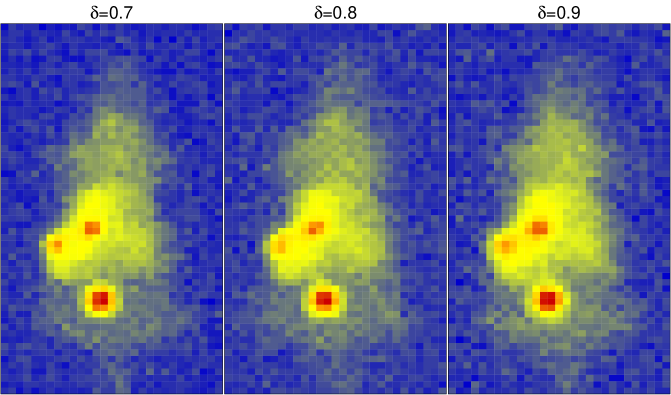
Figure S.1: Examples of data generated for the biomedical simulation study.

S.6 Archaeological Illustration Details

This section provides details on the design of the kernel matrix $\boldsymbol{K}$ utilised for the application to archaeological data and expressions for the VMP approximating densities used to fit the model with Skew Normal responses and Horseshoe penalization.

S.6.1 Kernel Matrix for Archaeological Data

Suppose all the magnetic features are located at the same depth below the surface, have the same vertical thickness and the susceptibility is constant along any vertical line through the features, but may vary between horizontal locations. We model the subsurface of the archaeological site as an ensemble of volume elements of equal size, called prisms, each having uniform susceptibility, fixed vertical depth (0.3m) and extent (0.5m), and a square cross section in the horizontal plane. Let $(x_{1},y_{1},z_{1})$ and $(x_{2},y_{2},z_{2})$ be the coordinates of opposite vertices of a prism with unit susceptibility, where the $x$, $y$ and $z$ axes point north, east and vertically downward, respectively. Then the vertical component of the anomaly due to the prism at a point with coordinates $(x,y,z)$ is

$$\Delta Z(x,y,z)=\frac{B}{4\pi}\left\{\big{[}\Delta Z^{(1)}+\Delta Z^{(2)}+\Delta Z^{(3)}\big{]}^{\zeta=z-z_{1}}_{\zeta=z-z_{2}}\right\},$$

where $B\approx 4.8\times 10^{4}$nT (nanoteslas) is the magnitude of the magnetic flux density due to the Earth’s field. The three additive components of $\Delta Z(x,y,z)$ are:

$$\Delta Z^{(1)}=\left[-\sin I\tan^{-1}\left(\frac{\xi\eta}{\zeta(\xi^{2}+\eta^{2}+\zeta^{2})^{1/2}}\right)\right]^{\xi=x-x_{1},\eta=y-y_{1}}_{\xi=x-x_{2},\eta=y-y_{2}},$$

$$\Delta Z^{(2)}=\left[\frac{1}{2}\cos I\cos\theta\log\left(\frac{(\xi^{2}+\eta^{2}+\zeta^{2})^{1/2}+\eta}{(\xi^{2}+\eta^{2}+\zeta^{2})^{1/2}-\eta}\right)\right]^{\xi=x-x_{1},\eta=y-y_{1}}_{\xi=x-x_{2},\eta=y-y_{2}},$$

$$\Delta Z^{(3)}=\left[\frac{1}{2}\cos I\sin\theta\log\left(\frac{(\xi^{2}+\eta^{2}+\zeta^{2})^{1/2}+\xi}{(\xi^{2}+\eta^{2}+\zeta^{2})^{1/2}-\xi}\right)\right]^{\xi=x-x_{1},\eta=y-y_{1}}_{\xi=x-x_{2},\eta=y-y_{2}},$$

where $I$ is the inclination of the Earth’s magnetic field and $\theta$ is the angle between the direction of magnetic north and the $x$ axis. In our application $I=65$°and $\theta=0$°.

The difference between two simultaneous readings from two sensors is recorded. One sensor is mounted vertically above the other at a distance of 0.5m. Then the recorded reading originated by a prism identified by coordinates $(x,y)$ is

$$h(x,y)=\Delta Z(x,y,z_{\tiny\mbox{U}})-\Delta Z(x,y,z_{\tiny\mbox{L}}),$$ (S.3)

where $z_{\tiny\mbox{U}}$ is the vertical coordinate of the upper sensor and $z_{\tiny\mbox{L}}$ is that of the lower sensor, which are held at 0.7m and 0.2m above the surface throughout the survey.

Suppose that a vector $\boldsymbol{y}$ of $n$ readings is recorded over a rectangular site at coordinates $\boldsymbol{s}_{j}$, $j=1,\ldots,n$. Assume that the subsurface is divided into a rectangular assemblage of $m$ prisms having coordinates $\boldsymbol{t}_{i}$, $i=1,\ldots,m$, and producing susceptibilities that are collected in an $m\times 1$ vector $\boldsymbol{x}$. Then the influence of the prism $i$ at surface location $j$ is

$$K_{ij}=h(\boldsymbol{t}_{i}-\boldsymbol{s}_{j})$$ (S.4)

where $h$ is the function defined in (S.3). The linear relationship between $\boldsymbol{y}$ and $\boldsymbol{x}$ is then modeled as $E(\boldsymbol{y})=\boldsymbol{K}\boldsymbol{x}$, where each element of the $n\times m$ matrix $\boldsymbol{K}$ is given by (S.4).

S.6.2 Approximating Density Functions

From (10) of Wand (2017), the densities of main interest, $q^{*}(\boldsymbol{x})$, $q^{*}(\sigma^{2}_{\varepsilon})$, $q^{*}(\lambda)$ and $q^{*}(\sigma^{2}_{x})$, have the following forms:

$$\begin{array}[]{c}q^{*}(\boldsymbol{x})\propto\exp\left\{\left[\begin{array}[]{c}\boldsymbol{x}\\[4.30554pt] \mathop{\mbox{\rm vec}}\big{(}\boldsymbol{x}\boldsymbol{x}^{T}\big{)}\end{array}\right]^{T}\mbox{\large$\boldsymbol{\eta}$}_{\mbox{\footnotesize$q(\boldsymbol{x})$}}\right\},\,\mbox{with}\,\,\mbox{\large$\boldsymbol{\eta}$}_{\mbox{\footnotesize$q(\boldsymbol{x})$}}\equiv\mbox{\large$\boldsymbol{\eta}$}_{\mbox{\footnotesize$p(\boldsymbol{x}|\boldsymbol{b},\sigma^{2}_{x})\rightarrow\boldsymbol{x}$}}+\mbox{\large$\boldsymbol{\eta}$}_{p(\boldsymbol{y}|\boldsymbol{x},\sigma^{2}_{\varepsilon},\lambda,\boldsymbol{c})\rightarrow\boldsymbol{x}},\end{array}$$

$$\begin{array}[]{c}q^{*}(\sigma^{2}_{\varepsilon})\propto\exp\left\{\left[\begin{array}[]{c}\log(\sigma^{2}_{\varepsilon})\\[5.16663pt] 1/\sigma_{\varepsilon}\\[5.16663pt] 1/\sigma^{2}_{\varepsilon}\end{array}\right]^{T}\mbox{\large$\boldsymbol{\eta}$}_{\mbox{\footnotesize$q(\sigma^{2}_{\epsilon})$}}\right\},\,\mbox{with}\,\,\mbox{\large$\boldsymbol{\eta}$}_{\mbox{\footnotesize$q(\sigma^{2}_{\epsilon})$}}\equiv\mbox{\large$\boldsymbol{\eta}$}_{p(\sigma^{2}_{\varepsilon})}+\mbox{\large$\boldsymbol{\eta}$}_{p(\boldsymbol{y}|\boldsymbol{x},\sigma^{2}_{\varepsilon},\lambda,\boldsymbol{c})\rightarrow\sigma^{2}_{\varepsilon}},\end{array}$$

$$\begin{array}[]{c}q^{*}(\lambda)\propto\exp\left\{\left[\begin{array}[]{c}\log(1+\lambda^{2})\\[4.30554pt] \lambda^{2}\\[4.30554pt] \lambda\sqrt{1+\lambda^{2}}\end{array}\right]^{T}\mbox{\large$\boldsymbol{\eta}$}_{q(\lambda)}\right\},\,\mbox{with}\,\,\mbox{\large$\boldsymbol{\eta}$}_{q(\lambda)}\equiv\mbox{\large$\boldsymbol{\eta}$}_{p(\lambda)}+\mbox{\large$\boldsymbol{\eta}$}_{p(\boldsymbol{y}|\boldsymbol{x},\sigma^{2}_{\varepsilon},\lambda,\boldsymbol{c})\rightarrow\lambda}\end{array}$$

$$\begin{array}[]{c}\mbox{and}\,\,q^{*}(\sigma^{2}_{x})\propto\exp\left\{\left[\begin{array}[]{c}\log(\sigma^{2}_{x})\\[5.16663pt] 1/\sigma^{2}_{x}\end{array}\right]^{T}\mbox{\large$\boldsymbol{\eta}$}_{\mbox{\footnotesize$q(\sigma^{2}_{x})$}}\right\},\,\mbox{with}\,\,\mbox{\large$\boldsymbol{\eta}$}_{\mbox{\footnotesize$q(\sigma^{2}_{x})$}}\equiv\mbox{\large$\boldsymbol{\eta}$}_{\mbox{\footnotesize$p(\sigma^{2}_{x}|a_{x})\rightarrow\sigma^{2}_{x}$}}+\mbox{\large$\boldsymbol{\eta}$}_{\mbox{\footnotesize$p(\boldsymbol{x}|\,\boldsymbol{b},\sigma^{2}_{x})\rightarrow\sigma^{2}_{x}$}}.\end{array}$$

Expressions for the other optimal approximating densities can be obtained in a similar manner. The full list of optimal approximating density functions respecting restriction (32) is the following:

$$q^{*}(\boldsymbol{x})\,\text{is a}\,N\big{(}\boldsymbol{\mu}_{q\left(\boldsymbol{x}\right)},\boldsymbol{\Sigma}_{q\left(\boldsymbol{x}\right)}\big{)}\,\text{density function},$$

$$q^{*}(c_{i})\propto\exp\left\{\left[\begin{array}[]{c}|c_{i}|\\[4.30554pt] c_{i}^{2}\\ \end{array}\right]^{T}\mbox{\large$\boldsymbol{\eta}$}_{c_{i}}\right\},\,\text{for a}\,2\times 1\,\text{natural paramter vector}\,\mbox{\large$\boldsymbol{\eta}$}_{c_{i}}\,\text{and}\,i=1,\ldots,m,$$

$$q^{*}(b_{j})\,\text{is an}\,\text{Inverse-Gaussian}\big{(}\mu_{q(b_{j})},\lambda_{q(b_{j})}\big{)}\,\text{density function, for}\,j=1,\ldots,d,$$

$$q^{*}(\sigma^{2}_{\varepsilon})\,\mbox{is an}\,\mbox{Inverse-Square-Root-Nadarajah}\left(\alpha_{q(\sigma^{2}_{\varepsilon})},\beta_{q(\sigma^{2}_{\varepsilon})},\gamma_{q(\sigma^{2}_{\varepsilon})}\right)\,\text{density function},$$

$$q^{*}(\lambda)\,\mbox{is a}\,\mbox{Sea-Sponge}\left(\alpha_{q(\lambda)},\beta_{q(\lambda)},\gamma_{q(\lambda)}\right)\,\text{density function},$$

$$q^{*}(\sigma^{2}_{x})\,\mbox{is an}\,\mbox{Inverse-}\chi^{2}\big{(}\kappa_{q\left(\sigma^{2}_{x}\right)},\lambda_{q\left(\sigma^{2}_{x}\right)}\big{)}\,\text{density function}$$

and $$q^{*}(a_{x})\,\mbox{is an}\,\mbox{Inverse-}\chi^{2}\big{(}\kappa_{q\left(a_{x}\right)},\lambda_{q\left(a_{x}\right)}\big{)}\,\text{density function}.$$

The common parameters of the $q$-densities of interest are:

$$\begin{array}[]{c}\boldsymbol{\mu}_{q\left(\boldsymbol{x}\right)}=\boldsymbol{\Sigma}_{q\left(\boldsymbol{x}\right)}\left(\mbox{\large$\boldsymbol{\eta}$}_{\mbox{\footnotesize$q(\boldsymbol{x})$}}\right)_{1:m},\,\,\,\boldsymbol{\Sigma}_{q\left(\boldsymbol{x}\right)}=-\frac{1}{2}\mathop{\mbox{\rm vec}}^{-1}\left\{\left(\mbox{\large$\boldsymbol{\eta}$}_{\mbox{\footnotesize$q(\boldsymbol{x})$}}\right)_{(m+1):m^{2}}\right\},\\[10.76385pt] \alpha_{q(\sigma^{2}_{\varepsilon})}=-2\left(1+\left(\mbox{\large$\boldsymbol{\eta}$}_{\mbox{\footnotesize$q(\sigma^{2}_{\epsilon})$}}\right)_{1}\right),\,\,\,\beta_{q(\sigma^{2}_{\varepsilon})}=-\left(\mbox{\large$\boldsymbol{\eta}$}_{\mbox{\footnotesize$q(\sigma^{2}_{\epsilon})$}}\right)_{3},\,\,\,\gamma_{q(\sigma^{2}_{\varepsilon})}=-\left(\mbox{\large$\boldsymbol{\eta}$}_{\mbox{\footnotesize$q(\sigma^{2}_{\epsilon})$}}\right)_{2},\\[10.76385pt] \alpha_{q(\lambda)}=\left(\mbox{\large$\boldsymbol{\eta}$}_{\mbox{\footnotesize$q(\lambda)$}}\right)_{1},\,\,\,\beta_{q(\lambda)}=-\left(\mbox{\large$\boldsymbol{\eta}$}_{\mbox{\footnotesize$q(\lambda)$}}\right)_{2},\,\,\,\gamma_{q(\lambda)}=\left(\mbox{\large$\boldsymbol{\eta}$}_{\mbox{\footnotesize$q(\lambda)$}}\right)_{3},\\[10.76385pt] \kappa_{q\left(\sigma^{2}_{x}\right)}=-2\left(1+\left(\mbox{\large$\boldsymbol{\eta}$}_{\mbox{\footnotesize$q(\sigma^{2}_{x})$}}\right)_{1}\right),\,\,\,\lambda_{q\left(\sigma^{2}_{x}\right)}=-2\left(\mbox{\large$\boldsymbol{\eta}$}_{\mbox{\footnotesize$q(\sigma^{2}_{x})$}}\right)_{2}.\end{array}$$

To obtain the common parameters of $q(\sigma^{2}_{\varepsilon})$ and $q(\sigma^{2}_{\lambda})$ from their natural parameters we make use of the results from Sections S.2.3 and S.2.5 of the supplementary material of McLean and Wand (2019) concerning the Inverse Square Root Nadarajah and Sea Sponge distributions.

Reference

Duong, T. (2018). ks: Kernel Smoothing (R package version 1.11.7).
https://CRAN.R-project.org/package=ks.