Generalized continuation Newton methods and the trust-region updating strategy for the underdetermined system

Abstract

This paper considers the generalized continuation Newton method and the trust-region updating strategy for the underdetermined system of nonlinear equations. Moreover, in order to improve its computational efficiency, the new method will not update the Jacobian matrix when the current Jacobian matrix performs well. The numerical results show that the new method is more robust and faster than the traditional optimization method such as the Levenberg-Marquardt method (a variant of trust-region methods, the built-in subroutine fsolve.m of the MATLAB R2020a environment). The computational time of the new method is about 1/8 to 1/50 of that of fsolve. Furthermore, it also proves the global convergence and the local superlinear convergence of the new method under some standard assumptions.

1 Introduction

In engineering fields, we often need to solve the underdetermined system of equations as follows:

$$F(x)=0,$$ (1)

where $F:\;\Re^{n}\to\Re^{m}$ and $m<n$. For example, this problem arises from finding the initial feasible point of the following differential-algebraic equations AP1998 ; BCP1996 ; HW1996 ; LF2000 ; LL2001 :

$$\frac{dx}{dt}=h(x,\,y),$$ (2)

$$g(x)=0.$$ (3)

Another case comes from the feasible direction method for solving the following nonlinearly constrained optimization problem NW1999 ; SY2006

$$\min_{x\Re^{n}}\;r(x)\;\text{subject to}\;c(x)=0,$$ (4)

where $r:\;\Re^{n}\to\Re$ and $c:\Re^{n}\to\Re^{m},\;m<n$.

The main difficulty of the undertermined system is the singularity $J(x)^{T}J(x)$ FY2005 ; Griewank1985 ; QACT2017 ; YF2001 , where $J=F^{\prime}$ is the Jacobian function of $F$. When $m=n$ and the Jacobian matrix $J(x)$ is nonsingular, there are many popular traditional optimization methods CGT2000 ; DS2009 ; Higham1999 ; Kelley2018 ; NW1999 ; Yuan1998 and the classical homotopy continuation methods AG2003 ; Doedel2007 ; OR2000 ; WSMMW1997 to solve it.

For the traditional optimization methods such as the trust-region methods and the line search methods, the solution $x^{\ast}$ of the nonlinear system (1) is found via solving the following equivalent nonlinear least-squares problem

$$\min_{x\in\Re^{n}}f(x)=\frac{1}{2}\|F(x)\|^{2},$$ (5)

where $\|\cdot\|$ denotes the Euclidean vector norm or its induced matrix norm throughout this paper. Generally speaking, the traditional optimization methods based on the merit function (5) are efficient for the large-scale problems when $J(x_{k})^{T}J(x_{k})\,(k=0,\,1,\,\ldots)$ are nonsingular, since they have the local superlinear convergence near the solution $x^{\ast}$ CGT2000 ; NW1999 .

However, the line search method based on the classical Gauss-Newton method will confront some problems when $J(x_{k})^{T}J(x_{k})$ is singular, since it obtains the search direction $d_{k}$ by solving the following linear equations:

$$J(x_{k})^{T}J(x_{k})d_{k}=-J(x_{k})^{T}F(x_{k}).$$

Furthermore, the termination condition

$$\|\nabla f(x_{k})\|=\|J(x_{k})^{T}F(x_{k})\|<\epsilon,$$ (6)

may lead the methods based on the merit function (5) to early stop far away from the solution $x^{\ast}$. This can be illustrated as follows. We consider

$$F(x)=Ax=0,\hskip 5.69054ptA=\begin{bmatrix}1&0\\ 0&10^{-6}\end{bmatrix}.$$ (7)

It is not difficult to know that the linear system (7) has a unique solution $x^{\ast}=(0,\,0)$. If we set $\epsilon=10^{-6}$, the traditional optimization methods will early stop far away from $x^{\ast}$ provided that $x_{k}=(0,\;c),\;c<10^{6}$.

For the classical homotopy methods, the solution $x^{\ast}$ of the nonlinear system (1) is found via constructing the following homotopy function

$$H(x,\,\lambda)=(1-\lambda)G(x)+\lambda F(x),$$ (8)

and attempting to trace an implicitly defined curve $\lambda(t)\in H^{-1}(0)$ from the starting point $(x_{0},\,0)$ to a solution $(x^{\ast},\,1)$ by the predictor-corrector methods AG2003 ; Doedel2007 , where the zero point of the artificial smooth function $G(x)$ is known. Generally speaking, the homotopy continuation methods are more reliable than the merit-function methods and they are very popular in engineering fields Liao2012 . The disadvantage of the classical homotopy methods is that they require significantly more function and derivative evaluations, and linear algebra operations than the merit-function methods since they need to solve many auxiliary nonlinear systems during the intermediate continuation process.

In order to overcome this shortcoming of the traditional homotopy methods, we consider the special continuation method based on the following generalized Newton flow AS2015 ; Branin1972 ; Davidenko1953 ; LXL2020 ; Tanabe1979

$$\frac{dx(t)}{dt}=-J(x)^{+}F(x),\;x(t_{0})=x_{0},$$ (9)

where $J(x)^{+}$ is the Moore-Penrose generalized inverse of the Jacobian matrix $J(x)$ (p. 11, SY2006 or p. 290, GV2013 ). Then, we construct a special ODE method with the adaptively time-stepping scheme based on the trust-region updating strategy to trace the trajectory of the generalized Newton flow (9). Consequently, we obtain a solution $x^{\ast}$ of the underdetermined nonlinear system (1).

The rest of this article is organized as follows. In the next section, we consider the generalized continuation Newton method with the adaptively time-stepping scheme and the updating technique of the Jacobian matrix based on the trust-region updating strategy for the underdetermined system of nonlinear equations. In section 3, under the standard assumptions, we prove the global convergence and the local superlinear convergence of the new method. In section 4, some promising numerical results of the new method are also reported, in comparison to the Levenberg-Marquardt method (a variant of the trust-region methods, the built-in subroutine fsolve.m of the MATLAB R2020a environment) FY2005 ; Levenberg1944 ; MATLAB ; Marquardt1963 ; More1978 ; YF2001 ). Finally, some conclusions and the discussions are given in section 5. Throughout this article, we assume that $F(\cdot)$ exists the zero point $x^{\ast}$.

2 Continuation Newton methods

In this section, based on the trust-region updating strategy, we construct an adaptively time-stepping scheme for the continuation Newton method to trace the trajectory of the generalized Newton flow and obtain its equilibrium point $x^{\ast}$.

2.1 The generalized continuous Newton flow

If we consider the damped Newton method with the line search strategy for the nonlinear system (1) Kelley2003 ; NW1999 , we have

$$x_{k+1}=x_{k}-\alpha_{k}J(x_{k})^{+}F(x_{k}).$$ (10)

We denote $o(\alpha)$ as the higher-order infinitesimal of $\alpha$, that is to say,

$$\lim_{\alpha\to 0}\frac{o(\alpha)}{\alpha}=0.$$

In equation (10), if we regard $x_{k}=x(t_{k})$ and $x_{k+1}=x(t_{k}+\alpha_{k})+o(\alpha_{k})$, we obtain the continuous Newton flow (9) when $\alpha_{k}\to 0$. Actually, if we apply an iteration with the explicit Euler method SGT2003 to the generalized Newton flow (9), we also obtain the damped Newton method (10). Since the rank of the Jacobian matrix $J(x)$ may be not full, we reformulate the generalized Newton flow (9) as the more general formula:

$$-J(x)\frac{dx(t)}{dt}=F(x),\hskip 5.69054ptx(t_{0})=x_{0}.$$ (11)

The continuous Newton flow (11) is an old method and can be backtracked to Davidenko’s work Davidenko1953 in 1953. After that, it was investigated by Branin Branin1972 , Deuflhard et al PHP1975 , Tanabe Tanabe1979 and Kalaba et al KZHH1977 in 1970s, and applied to nonlinear boundary problems by Axelsson and Sysala AS2015 recently. The continuous and even growing interest in this method originates from its some nice properties. One of them is that the solution $x(t)$ of the continuous Newton flow converges to the steady-state solution $x^{\ast}$ from any initial point $x_{0}$, as described by the following property 1.

Property 1

(Branin Branin1972 and Tanabe Tanabe1979 ) Assume that $x(t)$ is the solution of the continuous Newton flow (11), then $f(x(t))=\|F(x)\|^{2}$ converges to zero when $t\to\infty$. That is to say, for every limit point $x^{\ast}$ of $x(t)$, it is also a solution of the underdetermined system (1). Furthermore, every element $F^{i}(x)$ of $F(x)$ has the same convergence rate $e^{-t}$ and $x(t)$ can not converge to the solution $x^{\ast}$ of the underdetermined system (1) on the finite interval when the initial point $x_{0}$ is not a solution of the underdetermined system (1).

Proof.  Assume that $x(t)$ is the solution of the continuous Newton flow (11), then we have

$$\frac{d}{dt}\left(e^{t}F(x)\right)=e^{t}J(x)\frac{dx(t)}{dt}+e^{t}F(x)=0.$$

Consequently, we obtain

$$F(x(t))=F(x_{0})e^{-t}.$$ (12)

From equation (12), it is not difficult to know that every element $F^{i}(x)$ of $F(x)$ converges to zero with the linear convergence rate $e^{-t}$ when $t\to\infty$. Thus, if the solution $x(t)$ of the continuous Newton flow (11) belongs to a compact set, it has a limit point $x^{\ast}$ when $t\to\infty$, and this limit point $x^{\ast}$ is also a solution of the underdetermined system (1).

If we assume that the solution $x(t)$ of the continuous Newton flow (11) converges to the solution $x^{\ast}$ of the underdetermined system (1) on the finite interval $(0,\,T]$, from equation (12), we have

$$F(x^{\ast})=F(x_{0})e^{-T}.$$ (13)

Since $x^{\ast}$ is a solution of the underdetermined system (1), we have $F(x^{\ast})=0$. By substituting it into equation (13), we obtain

$$F(x_{0})=0.$$

Thus, it contradicts the assumption that $x_{0}$ is not a solution of the underdetermined system (1). Consequently, the solution $x(t)$ of the continuous Newton flow (11) can not converge to the solution $x^{\ast}$ of the underdetermined system (1) on the finite interval. ∎

Remark 1

The inverse $J(x)^{-1}$ of the Jacobian matrix $J(x)$ can be regarded as the preconditioner of $F(x)$ such that the solution elements $x_{i}(t)\,(i=1,\,2,\ldots,n)$ of the continuous Newton flow (9) have the roughly same convergence rates and it mitigates the stiff property of the ODE (9) (the definition of the stiff problem can be found in HW1996 and references therein). This property is very useful since it makes us adopt the explicit ODE method to trace the trajectory of the Newton flow.

Actually, if we consider $F(x)=Ax$, from the ODE (11), we have

$$A\frac{dx}{dt}=-Ax,\;x(0)=x_{0}.$$ (14)

By integrating the linear ODE (14), we obtain

$$x(t)=e^{-t}x_{0}.$$ (15)

From equation (15), we know that the solution $x(t)$ of the ODE (14) converges to zero exponentially with the same rate $e^{-t}$ when $t$ tends to infinity.

2.2 The generalized continuation Newton method

From subsection 2.1, we know that the solution $x(t)$ of the generalized continuous Newton flow (11) has the nice global convergence property. On the other hand, when the Jacobian matrix $J(x)$ is singular or nearly singular, the ODE (11) is the system of differential-algebraic equations (DAEs) and its trajectory can not be efficiently followed by the general ODE method such as the backward differentiation formulas (the built-in subroutine ode15s.m of the MATLAB environment AP1998 ; BCP1996 ; HW1996 ; MATLAB ; SGT2003 ). Thus, we need to construct the special method to handle this problem.

Since the continuous Newton flow (11) is intrinsically a nonlinear diminishing system for the energy function $f(x(t))=\|F(x(t))\|^{2}$, it can be integrated by the strong stability preserving methods GS1998 ; GST2001 and the steady-state solution $x^{\ast}$ can be obtained after the long time integration. Here, we consider another approach based on the traditional optimization methods for problem (11). We expect that the new method has the global convergence as the homotopy continuation method and the fast convergence rate near the steady-state solution $x^{\ast}$ as the merit-function method. In order to achieve these two aims, we construct the special continuation Newton method with the new step size $\alpha_{k}=\Delta t_{k}/(1+\Delta t_{k})$ and the time step size $\Delta t_{k}$ is adaptively adjusted by the trust-region updating strategy for problem (11).

Firstly, we apply the implicit Euler method to the continuous Newton flow (11) AP1998 ; BCP1996 , then we obtain

$$J(x_{k+1})\frac{x_{k+1}-x_{k}}{\Delta t_{k}} =-F(x_{k+1}).$$ (16)

The scheme (16) is an implicit method and it needs to solve a system of nonlinear equations at every iteration. To avoid solving the system of nonlinear equations, we replace $J(x_{k+1})$ with $J(x_{k})$ and substitute $F(x_{k+1})$ with its linear approximation $F(x_{k})+J(x_{k})(x_{k+1}-x_{k})$ in equation (16). Thus, we obtain the generalized continuation Newton method as follows:

$$J(x_{k})s_{k}^{N}=-F(x_{k}),\;x_{k+1}=x_{k}+\frac{\Delta t_{k}}{1+\Delta t_{k}}s_{k}^{N}.$$ (17)

The linear system (17) is underdetermined. That is to say, the row rank of $J(x_{k})$ is less than the number of the variable $s_{k}^{N}$. Thus, the linear system (17) may have many solutions or no solution. For simplicity, we assume that the Jacobian matrix $J(x_{k})$ is full row rank. That is to say, the row rank of $J(x_{k})$ equals $m$. In order to obtain the nearest point $x_{k+1}$ of $x_{k}$ under the constraint (17), we solve the following shortest distance problem:

$$\min_{s^{N}\in\Re^{n}}\;\left\|s^{N}\right\|^{2},\;\text{subject to}\;J_{k}s^{N}=-F_{k},$$ (18)

where $J_{k}$ equals $J(x_{k})$ or its approximation and $F_{k}=F(x_{k})$. By using the Lagrangian multiplier method SY2006 , it is not difficult to obtain the solution $s_{k}^{N}$ of problem (18) as follows:

$$s_{k}^{N}=-J_{k}^{+}F_{k},\;J_{k}^{+}=J_{k}^{T}\left(J_{k}J_{k}^{T}\right)^{-1},$$ (19)

where $J_{k}^{+}$ is the pseudo-inverse of $J_{k}$. Thus, from equations (17) and (19), we obtain the generalized continuation Newton method for the underdetermined system (1) as follows:

$$x_{k+1}=x_{k}-\frac{\Delta t_{k}}{1+\Delta t_{k}}J_{k}^{+}F_{k}.$$ (20)

The matrix $J_{k}J_{k}^{T}$ may be ill-conditioned. Thus, the Cholesky factorization method may fail to solve the linear system (19) for the large-scale problem. Therefore, we use the QR decomposition (pp. 247-248, GV2013 ) to solve it as follows:

$$J_{k}^{T}=Q_{k}R_{k},\;R_{k}^{T}d_{k}=-F_{k},\;s_{k}^{N}=Q_{k}d_{k},\;s_{k}=\frac{\Delta t_{k}}{1+\Delta t_{k}}s_{k}^{N},$$ (21)

where $Q_{k}\in\Re^{n\times m}$ satisfies $Q_{k}^{T}Q_{k}=I$ and $R_{k}\in\Re^{m\times m}$ is an upper triangle matrix.

Remark 2

The generalized continuation Newton method (20) is similar to the damped Newton method (10) if we let $\alpha_{k}=\Delta t_{k}/(1+\Delta t_{k})$ in equation (20). However, from the view of the ODE method, they are different. The damped Newton method (10) is obtained by the explicit Euler scheme applied to the generalized continuous Newton flow (11), and its time step size $\alpha_{k}$ is restricted by the numerical stability HW1996 ; SGT2003 . That is to say, for the linear test equation $dx/dt=-\lambda x$, its time step size $\alpha_{k}$ is restricted by the stable region $|1-\lambda\alpha_{k}|\leq 1$. Therefore, the large time step can not be adopted in the steady-state phase. The generalized continuation Newton method (20) is obtained by the implicit Euler method and its linear approximation applied to the continuous Newton flow (11), and its time step size $\Delta t_{k}$ is not restricted by the numerical stability. Therefore, the large time step can be adopted in the steady-state phase and it mimics the generalized Newton method near the solution $x^{\ast}$ such that it has the fast local convergence rate. The most of all, $\alpha_{k}=\Delta t_{k}/(\Delta t_{k}+1)$ in equation (20) is favourable to adopt the trust-region updating strategy for adaptively adjusting the time step size $\Delta t_{k}$ such that the generalized continuation Newton method (20) accurately traces the trajectory of the generalized continuous Newton flow in the transient-state phase and achieves the fast convergence rate near the equilibrium point $x^{\ast}$.

Remark 3

We denote $r(x)=\|F(x)\|$ and the generalized Newton direction $s_{k}^{N}$ as

$$s_{k}^{N}=-J(x_{k})^{+}F(x_{k}).$$ (22)

Then, when $F(x_{k})\neq 0$, we have

$$\nabla r(x_{k})^{T}s_{k}^{N}=-\frac{F(x_{k})^{T}J(x_{k})}{\|F(x_{k})\|}\left(J(x_{k})^{+}F(x_{k})\right)=-\|F(x_{k})\|<0.$$ (23)

That is to say, the generalized Newton direction $s_{k}^{N}$ is a descent direction of $r(x_{k})$.

2.3 The trust-region updating strategy

Another issue is how to adaptively adjust the time step size $\Delta t_{k}$ at every iteration. There is a popular way to control the time step size based on the trust-region updating strategy CGT2000 ; Deuflhard2004 ; Higham1999 ; Luo2009 ; Luo2010 ; LLT2007 ; LLS2021 ; LY2021 ; Yuan2015 . Its main idea is that the time step size $\Delta t_{k+1}$ will be enlarged when the linear model $F(x_{k})+J_{k}s_{k}$ approximates $F(x_{k}+s_{k})$ well, and $\Delta t_{k+1}$ will be reduced when $F(x_{k})+J_{k}s_{k}$ approximates $F(x_{k}+s_{k})$ badly.

In practice, we enlarge or reduce the time step size $\Delta t_{k}$ at every iteration according to the following ratio:

$$\rho_{k}=\frac{\|F(x_{k})\|-\|F(x_{k}+s_{k})\|}{\|F(x_{k})\|-\|F(x_{k})+J_{k}s_{k}\|}.$$ (24)

From the computational formula (20) of the search step $s_{k}$, we can save the computational time of the predicted model $F(x_{k})+J_{k}s_{k}$ by the following simplified formula:

$$F(x_{k})+J_{k}s_{k}=F(x_{k})-\frac{\Delta t_{k}}{1+\Delta t_{k}}F(x_{k})=\frac{1}{1+\Delta t_{k}}F(x_{k}).$$ (25)

Thus, from equations (24)-(25), we rewrite the computational formula (24) of $\rho_{k}$ as

$$\rho_{k}=\frac{\|F(x_{k})\|-\|F(x_{k}+s_{k})\|}{(\Delta t_{k}/(1+\Delta t_{k}))\|F(x_{k})\|}.$$ (26)

Therefore, according to the computation formula (26) of $\rho_{k}$ between the actual reduction and the predicted reduction, we give a particular adjustment strategy of $\Delta t_{k}$ as follows:

$$\Delta t_{k+1}=\begin{cases}\gamma_{1}\Delta t_{k},&{\text{if}\;\left|1-\rho_{k}\right|\leq\eta_{1},}\\ \Delta t_{k},&{\text{else if}\;\eta_{1}<\left|1-\rho_{k}\right|<\eta_{2},}\\ \gamma_{2}\Delta t_{k},&{\text{others},}\end{cases}$$ (27)

where the constants are selected as $\gamma_{1}=2,\;\gamma_{2}=0.5,\;\eta_{1}=0.25,\;\eta_{2}=0.75$, according to our numerical experiments.

Remark 4

This new time-stepping scheme based on the trust-region updating strategy has some advantages compared to the traditional line search strategy Luo2005 . If we use the line search strategy and the damped Newton method (10) to track the trajectory $z(t)$ of the generalized continuous Newton flow (11), in order to achieve the fast convergence rate in the steady-state phase, the time step size $\alpha_{k}$ of the damped Newton method is tried from 1 and reduced by half with many times at every iteration. Since the linear model $F(x_{k})+J(x_{k})s_{k}$ may not approximate $F(x_{k}+s_{k})$ well in the transient-state phase, the time step size $\alpha_{k}$ will be small. Consequently, the line search strategy consumes the unnecessary trial steps in the transient-state phase. However, the selection scheme of the time step size based on the trust-region updating strategy (26)-(27) can overcome this shortcoming.

2.4 The updating technique of the Jacobian matrix

For a system of nonlinear equations, the computational time of the Jacobian matrix is heavy if we update the Jacobian matrix $J(x_{k})$ at every iteration. In order to save the computational time of the Jacobian evaluation, similarly to the switching preconditioned technique LXLZ2021 , we set $J_{k+1}=J_{k}$ when $F_{k}+J_{k}s_{k}$ approximates $F(x_{k}+s_{k})$ well. Otherwise, we update $J_{k+1}=J(x_{k+1})$. An effective updating strategy is give by

$$J_{k+1}=\begin{cases}J_{k},\;\text{if}\;|1-\rho_{k}|\leq\eta_{1},\\ J(x_{k+1}),\;\text{otherwise},\end{cases}$$ (28)

where $\rho_{k}$ is defined by equation (26) and $\eta_{1}=0.25$. In practice, in order to save the computational time of decomposing the matrix $J_{k}$ when $J_{k-1}$ performs well, i.e. $|1-\rho_{k}|\leq\eta_{1}$, according to the updating formula (28), we set $R_{k}=R_{k-1}$ and $Q_{k}=Q_{k-1}$ in equation (21).

For a real-world problem, the analytical Jacobian $J(x_{k})$ may not be offered. Thus, in practice, we replace the Jacobian matrix $J(x_{k})$ with its difference approximation as follows:

$$J(x_{k})\approx\left[\frac{F(x_{k}+\epsilon e_{1})-F(x_{k})}{\epsilon},\,\ldots,\,\frac{F(x_{k}+\epsilon e_{n})-F(x_{k})}{\epsilon}\right],$$ (29)

where $e_{i}$ represents the unit vector whose elements equal zeros except for the $i$-th element which equals 1, and the parameter $\epsilon$ can be selected as $10^{-6}$ according to our numerical experiments.

According to the above discussions, we give the detailed implementation of the generalized continuation Newton method with the trust-region updating strategy for the underdetermined system of nonlinear equations in Algorithm 1.

Algorithm 1 Generalized continuation Newton methods and the trust-region updating strategy for the underdetermined system (The GCNMTr method)

0:     Function $F:\;\Re^{n}\to\Re^{m},\;m\leq n$, the initial point $x_{0}$ (optional), and the tolerance $\epsilon$ (optional).

0:     An approximation solution $x^{\ast}$ of nonlinear equations.

1:  Set the default $x_{0}=\text{ones}(n,\,1)$ and $\epsilon=10^{-6}$ when $x_{0}$ or $\epsilon$ is not provided by the calling subroutine.

2:  Initialize the parameters: $\eta_{a}=10^{-6},\;\eta_{1}=0.25,\;\gamma_{1}=2,\;\eta_{2}=0.75,\;\gamma_{2}=0.5,\;\text{maxit}=400$.

3:  Set $\Delta t_{0}=10^{-2}$, flag_success_trialstep = 1, $\text{itc}=0,\;k=0$.

4:  Evaluate $F_{k}=F(x_{k})$ and $J_{k}=J(x_{k})$.

5:  By using the qr decomposition $[Q_{k},R_{k}]=\text{qr}(J_{k}^{T})$ of $J_{k}^{T}$, we obtain the orthogonal matrix $Q_{k}$ and the upper triangle matrix $R_{k}$.

6:  Set $\rho_{k}=1$.

7:  while (itc $<$ maxit) do

8:     if (flag_success_trialstep == 1) then

9:        Set itc = itc + 1.

10:        Compute $\text{Res}_{k}=\|F_{k}\|_{\infty}$.

11:        if ($\text{Res}_{k}<\epsilon$) then

12:           break;

13:        end if

14:        if $(|1-\rho_{k}|>0.25)$ then

15:           Evaluate $J_{k}=J(x_{k})$.

16:           By using the qr decomposition $[Q_{k},R_{k}]=\text{qr}(J_{k}^{T})$ of $J_{k}^{T}$, we obtain the orthogonal matrix $Q_{k}$ and the upper triangle matrix $R_{k}$.

17:        end if

18:        By solving $R_{k}^{T}b_{k}=-F_{k}$ and $s_{k}^{N}=Q_{k}b_{k}$, we obtain the Newton step $s_{k}^{N}$.

19:     end if

20:     Set $s_{k}={\Delta t_{k}}/{(1+\Delta t_{k})}\,s_{k}^{N},\;x_{k+1}=x_{k}+s_{k}$.

21:     Evaluate $F(x_{k+1})$.

22:     if $\left(\|F_{k}\|<\|F_{k}+J_{k}s_{k}\|\right)$ then

23:        $\rho_{k}=-1$;

24:     else

25:        Compute the ratio $\rho_{k}$ from equation (26).

26:     end if

27:     Adjust the time step size $\Delta t_{k+1}$ according to the trust-region updating strategy (27).

28:     if $(\rho_{k}\geq\eta_{a})$ then

29:        Accept the trial point $x_{k+1}$. Set flag_success_trialstep = 1.

30:     else

31:        Set $x_{k+1}=x_{k}$, $F_{k+1}=F_{k}$, $s_{k+1}^{N}=s_{k}^{N}$, flag_success_trialstep = 0.

32:     end if

33:     Set $\rho_{k+1}=\rho_{k}$, $R_{k+1}=R_{k}$, $Q_{k+1}=Q_{k}$.

34:     Set $k\longleftarrow k+1$.

35:  end while

3 Algorithm analysis

In this section, we discuss some theoretical properties of Algorithm 1. Firstly, we estimate the lower bound of the predicted reduction $\|F(x_{k})\|-\|F(x_{k})+J_{k}s_{k}\|$, which is similar to that of the trust-region method for the unconstrained optimization problem Powell1975 .

According to the theorem of the singular value decomposition (pp. 76, GV2013 ), for the matrix $J_{k}\in\Re^{m\times n}$, there exist orthogonal matrices $U_{k}\in\Re^{m\times m}$ and $V_{k}\in\Re^{n\times n}$ such that

$$U_{k}^{T}J_{k}V_{k}=\Sigma_{k}=\text{diag}\left(\sigma_{k}^{1},\,\ldots,\,\sigma_{k}^{m}\right)\in\Re^{m\times n},$$ (30)

where $\sigma_{k}^{1}\geq\sigma_{k}^{2}\geq\cdots\geq\sigma_{k}^{m}\geq 0$.

Lemma 1

Assume that it exists a positive constant $c_{\sigma}$ such that

$$\sigma_{k}^{min}\geq c_{\sigma}$$ (31)

holds for all $k=0,\,1,\ldots$, where $\sigma_{k}^{min}=\sigma_{k}^{m}$ is the smallest singular value of $J_{k}\in\Re^{m\times n}$. Furthermore, we suppose that $s_{k}$ is the solution of the generalized continuation Newton method (19)-(20). Then, we have the following estimation

$$\|F(x_{k})\|-\|F(x_{k})+J_{k}s_{k}\|=\frac{\Delta t_{k}}{1+\Delta t_{k}}\|F(x_{k})\|.$$ (32)

Proof.  From equations (30)-(31), we have

$$J_{k}^{+}=J_{k}^{T}\left(J_{k}J_{k}^{T}\right)^{-1}=V_{k}^{T}\Sigma_{k}^{-1}U_{k},\;\Sigma_{k}^{-1}=\text{diag}\left({1}/{\sigma_{k}^{1}},\,\ldots,\,{1}/{\sigma_{k}^{m}}\right)\in\Re^{n\times m}.$$ (33)

Thus, from equations (20), (30) and (33), we have

$$\|F(x_{k})+J_{k}s_{k}\|=\|J_{k}s_{k}+F_{k}\|=\left\|-\frac{\Delta t_{k}}{1+\Delta t_{k}}J_{k}J_{k}^{+}F_{k}+F_{k}\right\|=\frac{1}{1+\Delta t_{k}}\|F_{k}\|.$$ (34)

Therefore, from equation (34), we obtain the estimation (32). ∎

In order to prove that the sequence $\{\|F(x_{k})\|\}$ converges to zero when $k$ tends to infinity, we also need to estimate the lower bound of the time step size $\Delta t_{k}$.

Lemma 2

Assume that $F:\;\Re^{n}\to\Re^{m}$ is continuously differentiable and its Jacobian function $J$ is Lipschitz continuous. That is to say, it exists a positive number $L$ such that

$$\|J(x)-J(y)\|\leq L\|x-y\|,\;\forall x,\,y\in\Re^{n}.$$ (35)

Furthermore, we suppose that the sequence $\{x_{k}\}$ is generated by Algorithm 1 and the condition (31) holds for all $J_{k}\,(k=0,\,1,\,\ldots)$. Then, there exists a positive number $\delta_{\Delta t}$ such that

$$\Delta t_{k}\geq\gamma_{2}\delta_{\Delta t}>0$$ (36)

holds for $k=0,\,1,\,2,\,\ldots$, where $\Delta t_{k}$ is adaptively adjusted by formulas (26)-(27).

Proof.  We prove this result by distinguishing two different cases, i.e. $J_{k}=J(x_{k})$ or $J_{k}=J_{k-1}$. (i) Firstly, we consider the case of $J_{k}=J(x_{k})$. From the Lipschitz continuous assumption (35) of $J(\cdot)$, we have

$$\left\|F(x_{k}+s_{k})-F(x_{k})-J(x_{k})s_{k}\right\|=\left\|\int_{0}^{1}J(x_{k}+ts_{k})s_{k}dt-J(x_{k})s_{k}\right\|$$

$$=\left\|\int_{0}^{1}(J(x_{k}+ts_{k})-J(x_{k}))s_{k}dt\right\|\leq\int_{0}^{1}\|(J(x_{k}+ts_{k})-J(x_{k}))s_{k}\|dt$$

$$\leq\int_{0}^{1}\|J(x_{k}+ts_{k})-J(x_{k})\|\|s_{k}\|dt\leq\int_{0}^{1}L\|s_{k}\|^{2}tdt=\frac{1}{2}L\|s_{k}\|^{2}.$$ (37)

On the other hand, from equations (19), (31) and (33), we have

$$\|s_{k}\|=\frac{\Delta t_{k}}{1+\Delta t_{k}}\left\|-J_{k}^{+}F_{k}\right\|\leq\frac{\Delta t_{k}}{c_{\sigma}(1+\Delta t_{k})}\|F_{k}\|.$$ (38)

Thus, from equations (37)-(38), we obtain

$$\left\|F(x_{k}+s_{k})-F(x_{k})-J(x_{k})s_{k}\right\|\leq\frac{L}{2c_{\sigma}^{2}}\left(\frac{\Delta t_{k}}{1+\Delta t_{k}}\right)^{2}\|F_{k}\|^{2}.$$ (39)

From the definition (26) of $\rho_{k}$, the estimation (32), and equation (39), we obtain

$$|\rho_{k}-1|=\left|\frac{\|F(x_{k})\|-\|F(x_{k}+s_{k})\|}{\|F(x_{k})\|-\|F(x_{k})+J(x_{k})s_{k}\|}-1\right|$$

$$\hskip 5.69054pt\leq\frac{\|F(x_{k}+s_{k})-F(x_{k})-J(x_{k})s_{k}\|}{\|F(x_{k})\|-\|F(x_{k})+J(x_{k})s_{k}\|}\leq\frac{L}{2c_{\sigma}^{2}}\frac{\Delta t_{k}}{1+\Delta t_{k}}\|F_{k}\|\leq\frac{L}{2c_{\sigma}^{2}}\|F_{k}\|.$$ (40)

According to Algorithm 1, we know that the sequence $\{\|F(x_{k})\|\}$ is monotonically decreasing. Consequently, we have $\|F(x_{k})\|\leq\|F(x_{0})\|,\;k=1,\,2,\,\dots$. We denote

$$\delta_{\Delta t}\triangleq\min\left\{\frac{2c_{\sigma}^{2}}{\|F(x_{0})\|L}\eta_{1},\;\Delta t_{0}\right\}.$$ (41)

Thus, from equations (40)-(41), we obtain $|\rho_{k}-1|\leq\eta_{1}$ when $\Delta t_{k}\leq\delta_{\Delta t}$. Consequently, according to the time-stepping scheme (27), $\Delta t_{k+1}$ will be enlarged.

(ii) The other case is $J_{k}=J_{k-1}$. When $J_{k}=J_{k-1}$, from equation (28), we know $|1-\rho_{k-1}|\leq\eta_{1}$. Consequently, according to the time-stepping scheme (27), $\Delta t_{k}$ will be greater than $\Delta t_{k-1}$, i.e. $\Delta t_{k}=\gamma_{1}\Delta t_{k-1}$.

Assume that $K$ is the first index such that $\Delta t_{K}\leq\delta_{\Delta t}$. Then, from equation (28) and the above discussions, we know that $J_{K}=J(x_{K})$. Otherwise, from the discussion of the case (ii), we know $\Delta t_{K-1}<\Delta t_{K}$, which contradicts the assumption that $K$ is the first index such that $\Delta t_{K}\leq\delta_{\Delta t}$. Therefore, from equations (40)-(41), we obtain $|\rho_{K}-1|\leq\eta_{1}$. Consequently, $\Delta t_{K+1}$ will be enlarged according to the adaptive adjustment scheme (27). Consequently, $\Delta t_{k}\geq\gamma_{2}\delta_{\Delta t}$ holds for all $k=0,\,1,\,2,\,\dots$. ∎

By using the estimate results of Lemma 1 and Lemma 2, we can prove that the sequence $\{\|F(x_{k})\|\}$ converges to zero when $k$ tends to infinity.

Theorem 3.1

Assume that $F:\;\Re^{n}\to\Re^{m}$ is continuously differentiable and its Jacobian function $J$ satisfies the Lipschitz condition (35). Furthermore, we suppose that the sequence $\{x_{k}\}$ is generated by Algorithm 1 and the Jacobian matrix $J_{k}$ satisfies the condition (31). Then, we have

$$\lim_{k\to\infty}\inf\;\|F(x_{k})\|=0.$$ (42)

Proof.  According to Algorithm 1 and Lemma 2, we know that there exists an infinite subsequence $\{x_{k_{l}}\}$ such that

$$\frac{\|F(x_{k_{l}})\|-\|F(x_{k_{l}}+s_{k_{l}})\|}{\|F(x_{k_{l}})\|-\|F(x_{k_{l}})+J_{k_{l}}s_{k_{l}}\|}\geq\eta_{2}$$ (43)

holds for all $l=0,\,1,\,2,\,\ldots$. Otherwise, all steps are rejected after a given iteration index, then the time step size will keep decreasing, which contradicts equation (36).

From equations (32), (43) and (36), we have

$$\|F(x_{k_{l}})\|-\|F(x_{k_{l}}+s_{k_{l}})\|\geq\eta_{2}\frac{\Delta t_{k_{l}}}{1+\Delta t_{k_{l}}}\|F(x_{k_{l}})\|\geq\eta_{2}\frac{\gamma_{2}\delta_{\Delta t}}{1+\gamma_{2}\delta_{\Delta t}}\|F(x_{k_{l}})\|.$$ (44)

Therefore, from equation (44) and $\|F(x_{k+1})\|\leq\|F(x_{k})\|$, we have

$$\|F(x_{0})\|\geq\|F(x_{0})\|-\lim_{k\to\infty}\|F(x_{k})\|=\sum_{k=0}^{\infty}(\|F(x_{k})\|-\|F(x_{k+1})\|)$$

$$\hskip 5.69054pt\geq\sum_{l=0}^{\infty}(\|F(x_{k_{l}})\|-\|F(x_{k_{l}}+s_{k_{l}})\|)\geq\eta_{2}\frac{\gamma_{2}\delta_{\Delta t}}{1+\gamma_{2}\delta_{\Delta t}}\sum_{l=0}^{\infty}\|F(x_{k_{l}})\|.$$ (45)

Consequently, from equation (45), we obtain

$$\lim_{l\to\infty}\|F(x_{k_{l}})\|=0.$$

That is to say, the result (42) is true. ∎

Under the full row rank of $J(x^{\ast})$ and the local Lipschitz continuity (35), we analyze the local superlinear convergence of Algorithm 1 near the solution $x^{\ast}$. The framework of its proof can be roughly described as follows. Firstly, we prove that the sequence $\{x_{k}\}$ converges to $x^{\ast}$ when $x_{0}$ comes close enough to the solution $x^{\ast}$. Then, we prove $\lim_{k\to\infty}\Delta t_{k}=\infty$. Finally, we prove that the search step $s_{k}$ approximates the Newton step $s_{k}^{N}$. Consequently, the sequence $\{x_{k}\}$ superlinearly converges to $x^{\ast}$.

For convenience, we define the neighbourhood $B_{\delta}(x^{\ast})$ of $x^{\ast}$ as

$$B_{\delta}(x^{\ast})=\{x:\|x-x^{\ast}\|\leq\delta\}.$$ (46)

Lemma 3

Assume that $F:\;\Re^{n}\to\Re^{m}$ is continuously differentiable and $F(x^{\ast})=0$. Furthermore, we suppose that its Jacobian function $J$ satisfies the Lipschitz continuity (35) and the condition (31) when $x\in B_{\delta}(x^{\ast})$. Then, there exists a neighborhood $B_{r}(x^{\ast})$ of $x^{\ast}$ such that the sequence $\{x_{k}\}$ generated by Algorithm 1 with $x_{0}\in B_{r}(x^{\ast})$ converges to $x^{\ast}$.

Proof.  From equations (30)-(31), we obtain the generalized inverse $J_{k}^{+}$ in equation (33) and its estimation

$$\left\|J_{k}^{+}\right\|\leq{1}/{c_{\sigma}},\;k=0,\,1,\,2,\ldots.$$ (47)

We denote $e_{k}=x_{k}-x^{\ast}$. When $s_{k}$ is not an accepted step, we obviously have $e_{k+1}=e_{k}$. Therefore, we consider the case that $s_{k}$ is an accepted step. When $s_{k}$ is an accepted step, from the generalized continuation Newton method (20), we have

$$e_{k+1} =e_{k}+s_{k}=e_{k}+\frac{\Delta t_{k}}{1+\Delta t_{k}}J_{k}^{+}(F(x_{k})-F(x^{\ast}))$$

$$=e_{k}+\frac{\Delta t_{k}}{1+\Delta t_{k}}J_{k}^{+}\int_{0}^{1}J(x^{\ast}+te_{k})e_{k}dt.$$ (48)

By rearranging the above equation (48), we obtain

$$e_{k+1}=\frac{1}{1+\Delta t_{k}}e_{k}+\frac{\Delta t_{k}}{1+\Delta t_{k}}J_{k}^{+}\int_{0}^{1}\left(J(x^{\ast}+te_{k})-J(x_{k})\right)e_{k}dt.$$

By using the Lipschitz continuity (35) of $J$ and the estimation (47), we have

$$\|e_{k+1}\|\leq\frac{1}{1+\Delta t_{k}}\|e_{k}\|+\frac{\Delta t_{k}}{1+\Delta t_{k}}\left\|J_{k}^{+}\right\|\int_{0}^{1}\left\|J(x^{\ast}+te_{k})-J(x_{k})\right\|\|e_{k}\|dt$$

$$\hskip 5.69054pt\leq\frac{1}{1+\Delta t_{k}}\|e_{k}\|+\frac{\Delta t_{k}}{1+\Delta t_{k}}\frac{L}{2c_{\sigma}}\|e_{k}\|^{2}=\frac{1+L/(2c_{\sigma})\|e_{k}\|{\Delta t_{k}}}{1+\Delta t_{k}}\|e_{k}\|.$$ (49)

We denote

$$q_{k}\triangleq\frac{1+L/(2c_{\sigma})\|e_{k}\|{\Delta t_{k}}}{1+\Delta t_{k}},$$ (50)

and select $x_{0}\in B_{\delta}(x^{\ast})$ to satisfy

$$\|e_{0}\|<\frac{c_{\sigma}}{L}.$$ (51)

We denote $r=\min\{\delta,\,2c_{\sigma}/L\}$. When $x_{0}\in B_{r}(x^{\ast})$, from equations (49)-(51), by induction, we have

$$\|e_{k+1}\|\leq q_{k}\|e_{k}\|,\;q_{k}<\frac{1+(1/2)\Delta t_{k}}{1+\Delta t_{k}}<1.$$ (52)

It is not difficult to know that $f(t)\triangleq(1+\alpha t)/(1+t)$ is monotonically decreasing when $0\leq\alpha<1$. Thus, from the estimation (36) of the time step size $\Delta t_{k}$ and equation (52), we obtain

$$\|e_{k+1}\|\leq q_{k}\|e_{k}\|\leq q\|e_{k}\|,\;q\triangleq\frac{1+(1/2)\gamma_{2}\delta_{\Delta t}}{1+\gamma_{2}\delta_{\Delta t}}<1.$$ (53)

Consequently, from equation (53), we know that $e_{k+1}\leq e_{k}$ holds for all $k=0,\,1,\,2,\,\ldots$, since $e_{k+1}=e_{k}$ when $s_{k}$ is not an accepted step. According to Algorithm LABEL:GCNMTR and Lemma 2, we know that there exists an infinite subsequence $\{x_{k_{l}}\}$ such that $s_{k_{l}}\,(l=0,\,1,\,\ldots)$ are all accepted steps. Otherwise, all steps are rejected after a given iteration index, then the time step size will keep decreasing, which contradicts equation (36). Therefore, from equation (53) and $e_{k}\leq e_{k+1}$, we have

$$e_{k_{l}}\leq q\,e_{k_{l-1}}\leq\cdots\leq q^{l}e_{k_{0}}.$$

That is to say, we have $\lim_{l\to\infty}e_{k_{l}}=0$. By combining it with $e_{k+1}\leq e_{k}$, we obtain $\lim_{k\to\infty}x_{k}=x^{\ast}$. ∎

Lemma 4

Assume that $F:\;\Re^{n}\to\Re^{m}$ is continuously differentiable and $F(x^{\ast})=0$. Furthermore, we suppose that its Jacobian function $J$ satisfies the Lipschitz continuity (35) and the condition (31) when $x\in B_{\delta}(x^{\ast})$. Then, there exists a neighborhood $B_{r}(x^{\ast})$ of $x^{\ast}$ such that the sequence $\{x_{k}\}$ generated by Algorithm 1 with $x_{0}\in B_{r}(x^{\ast})$ converges to $x^{\ast}$ and the generated time step $\Delta t_{k}$ tends to infinity.

Proof.  The first part of the lemma is proved in Lemma 3, i.e. $\lim_{k\to\infty}x_{k}=x^{\ast}$. Now, we prove the second part of the lemma, i.e. $\lim_{k\to\infty}\Delta t_{k}=\infty$.

We can assume that there exists an infinite subsequence $\{x_{k_{l}}\}$ such that $J_{k_{l}}=J(x_{k_{l}})$ holds for all $l=0,\,1,\ldots$. Otherwise, according to equation (28), all Jacobian matrices $J_{k}\,(k=K+1,\,K+2,\,\ldots)$ equal $J_{K}$ and $|\rho_{k}-1|\leq\eta_{1}\,(k=K,\,K+2,\,\ldots)$ after a given iteration index $K$. Then, according to the time-stepping scheme (27), we obtain $\Delta t_{k+1}=\gamma_{1}\Delta t_{k}\,(k=K,\,K+1,\,\ldots)$. Consequently, we have $\lim_{k\to\infty}\Delta t_{k}=\infty$. That is to say, for this case, the second part of the lemma also is proved.

Since $J_{k_{l}}=J(x_{k_{l}})$, from equations (20) and (47), we have

$$\|s_{k_{l}}\|=\frac{\Delta t_{k_{l}}}{1+\Delta t_{k_{l}}}\left\|J_{k_{l}}^{+}F(x_{k_{l}})\right\|\leq\frac{\Delta t_{k_{l}}}{1+\Delta t_{k_{l}}}\|J_{k_{l}}^{+}\|\|F(x_{k_{l}})\|$$

$$\hskip 5.69054pt\leq\frac{\Delta t_{k_{l}}}{c_{\sigma}(1+\Delta t_{k_{l}})}\|F(x_{k_{l}})\|.$$ (54)

Similarly to the estimation (40), from the definition (26) of $\rho_{k_{l}}$, inequalities (32) and (54), we have

$$|\rho_{k_{l}}-1|=\left|\frac{\|F(x_{k_{l}})\|-\|F(x_{k_{l}}+s_{k_{l}})\|}{\|F(x_{k_{l}})\|-\|F(x_{k_{l}})+J(x_{k_{l}})s_{k_{l}}\|}-1\right|$$

$$\hskip 5.69054pt\leq\frac{L}{2c_{\sigma}^{2}}\left(\frac{\Delta t_{k_{l}}}{1+\Delta t_{k_{l}}}\right)\|F(x_{k_{l}})\|\leq\frac{L}{2c_{\sigma}^{2}}\|F(x_{k_{l}})\|.$$ (55)

Since $\lim_{k\to\infty}x_{k}=x^{\ast}$ and $F(x^{\ast})=0$, we can select a sufficiently large number $K$ such that

$$\|F(x_{K})\|\leq\frac{2\eta_{1}c_{\sigma}^{2}}{3L}.$$ (56)

From inequalities (55)-(56) and the monotonically decreasing property $\|F(x_{k+1})\|\leq\|F(x_{k})\|$, we have $|\rho_{k_{l}}-1|\leq\eta_{1}$ when $k_{l}\geq K$. This means $\Delta t_{{k_{l}}+1}=\gamma_{1}\Delta t_{k_{l}}$ according to the time-stepping scheme (27).

Now, we consider the $(k_{l}+1)$-th iteration. From equation (28), we know that $J_{{k_{l}}+1}=J_{k_{l}}=J(x_{k_{l}})$. Then, from the definition (26) of $\rho_{{k_{l}}+1}$, equation (32) and the Lipschitz continuity (35), we have

$$|\rho_{{k_{l}}+1}-1|=\left|\frac{\|F(x_{{k_{l}}+1})\|-\|F(x_{{k_{l}}+1}+s_{{k_{l}}+1})\|}{\|F(x_{{k_{l}}+1})\|-\|F(x_{{k_{l}}+1})+J_{{k_{l}}+1}s_{{k_{l}}+1}\|}-1\right|$$

$$\hskip 5.69054pt\leq\frac{\|F(x_{{k_{l}}+1}+s_{{k_{l}}+1})-F(x_{{k_{l}}+1})-J_{{k_{l}}+1}s_{{k_{l}}+1}\|}{\|F(x_{{k_{l}}+1})\|-\|F(x_{{k_{l}}+1})+J_{{k_{l}}+1}s_{{k_{l}}+1}\|}$$

$$\hskip 5.69054pt=\frac{\|\int_{0}^{1}(J(x_{{k_{l}}+1}+ts_{{k_{l}}+1})-J(x_{k_{l}}))s_{{k_{l}}+1}dt\|}{\|F(x_{{k_{l}}+1})\|-\|F(x_{{k_{l}}+1})+J_{{k_{l}}+1}s_{{k_{l}}+1}\|}$$

$$\hskip 5.69054pt\leq\frac{1+\Delta t_{{k_{l}}+1}}{\Delta t_{{k_{l}}+1}}\frac{L\left(0.5\|s_{{k_{l}}+1}\|^{2}+\|s_{{k_{l}}+1}\|\|s_{k_{l}}\|\right)}{\|F(x_{{k_{l}}+1})\|}.$$ (57)

By substituting equation (54) into equation (57), we obtain

$$|\rho_{{k_{l}}+1}-1|\leq\frac{L\;\Delta t_{{k_{l}}+1}}{c_{\sigma}^{2}(1+\Delta t_{{k_{l}}+1})}\left(0.5\|F(x_{{k_{l}}+1})\|+\|F(x_{k_{l}})\|\right)\leq\frac{3L}{2c_{\sigma}^{2}}\|F(x_{k_{l}})\|,$$ (58)

where the property $\|F(x_{{k_{l}}+1})\|\leq\|F(x_{k_{l}})\|$ is used in the last inequality.

From equations (56) and (58), we have $|\rho_{{k_{l}}+1}-1|\leq\eta_{1}$. This means $\Delta t_{{k_{l}}+2}=\gamma_{1}\Delta t_{{k_{l}}+1}=\gamma_{1}^{2}\Delta t_{k_{l}}$ according to the time-stepping scheme (27). Thus, for the $(k_{l}+2)$ iteration, when $|\rho_{{k_{l}}+2}-1|>\eta_{1}$, according to the time-stepping scheme (27), we have $\Delta t_{{k_{l}}+3}\geq\gamma_{2}\gamma_{1}^{2}\Delta t_{k_{l}}=\gamma_{1}\Delta t_{k_{l}}$ (Here, we select $\gamma_{1}=2$ and $\gamma_{2}=1/2$). Furthermore, from equation (28), we know $J_{{k_{l}}+3}=J(x_{{k_{l}}+3})$ at the $({k_{l}}+3)$-th iteration. Similarly to the estimation $|\rho_{k_{l}}-1|\leq\eta_{1}$ of $J_{k_{l}}=J(x_{k_{l}})$, we have $|\rho_{{k_{l}}+3}-1|\leq\eta_{1}$. This means $\Delta t_{{k_{l}}+4}=\gamma_{1}\Delta t_{{k_{l}}+3}\geq\gamma_{1}^{2}\Delta t_{k_{l}}$ according to the time-stepping scheme (27). Thus, the subsequent iterations start a new cycle for the time step size.

When $|\rho_{{k_{l}}+2}-1|\leq\eta_{1}$, according to the time-stepping scheme (27), we have $\Delta t_{{k_{l}}+3}=\gamma_{1}\Delta t_{{k_{l}}+2}=\gamma_{1}^{3}\Delta t_{k_{l}}$ and the time steps keep increasing until $|\rho_{{k_{l}}+m}-1|>\eta_{1}\,(m=3,\,4,\,\ldots)$. Then, the subsequent iterations start a new cycle for the time step size.

By combining the above discussions of two cases $|\rho_{{k_{l}}+2}-1|>\eta_{1}$ or $|\rho_{{k_{l}}+2}-1|\leq\eta_{1}$, we know $\Delta t_{k_{l}}\geq\gamma_{1}\Delta t_{k_{l+1}}$ and $\Delta t_{{k_{l}}+m}\geq\Delta t_{k_{l}}$ when $0\leq m\leq k_{l+1}-k_{l}$. Consequently, we obtain $\lim_{l\to\infty}\Delta t_{k_{l}}=\infty$. By combining the property $\Delta t_{{k_{l}}+m}\geq\Delta t_{k_{l}}\,(0\leq m\leq k_{l+1}-k_{l})$, we obtain $\lim_{k\to\infty}\Delta t_{k}=\infty$. ∎

Theorem 3.2

Assume that $F:\;\Re^{n}\to\Re^{m}$ is continuously differentiable and $F(x^{\ast})=0$. Furthermore, we suppose that its Jacobian function $J$ satisfies the Lipschitz continuity (35) and the condition (31) when $x\in B_{\delta}(x^{\ast})$. Then, there exists a neighborhood $B_{r}(x^{\ast})$ of $x^{\ast}$ such that the sequence $\{x_{k}\}$ generated by Algorithm 1 with $x_{0}\in B_{r}(x^{\ast})$ converges superlinearly to $x^{\ast}$.

Proof.  From Lemma 3 and Lemma 4, we know $\lim_{k\to\infty}x_{k}=x^{\ast}$ and $\lim_{k\to\infty}\Delta t_{k}=\infty$. Firstly, we prove that there are only finite steps which are rejected. That is to say, all steps are accepted after a given iteration index.

We assume that there exist the infinite rejected steps. Since $\lim_{k\to\infty}x_{k}=x^{\ast}$ and $F(x^{\ast})=0$, we can select a sufficiently large number $K_{1}$ such that

$$\|F(x_{K_{1}})\|\leq\frac{\eta_{1}c_{\sigma}^{2}}{L}.$$ (59)

Furthermore, there exists a positive $K_{2}$ such that

$$\|x_{k}-x_{l}\|\leq\frac{\eta_{1}c_{\sigma}}{2L},\;\forall k,\,l\geq K_{2}.$$ (60)

We denote $K=\max\{K_{1},\,K_{2}\}$. For the $k$-th iteration, we assume that $s_{l-1}\,(l\leq k)$ is the step such that $|\rho_{l-1}-1|<\eta_{1}$ holds and its index $l$ is the closest to $k$. Then, we have $J_{k}=J_{l}=J(x_{l})$ according to equation (28).

Similarly to the estimation (57), from the definition (26) of $\rho_{k}$, equation (20) and the Lipschitz continuity (35), we have

$$|\rho_{k}-1|\leq\frac{1+\Delta t_{k}}{\Delta t_{k}}\frac{L\left(0.5\|s_{k}\|^{2}+\|s_{k}\|\|x_{k}-x_{l}\|\right)}{\|F(x_{k})\|}.$$ (61)

By substituting equation (38) into equation (61), we obtain

$$|\rho_{k}-1|\leq\frac{L}{c_{\sigma}}\left(\frac{1}{2c_{\sigma}}\frac{\Delta t_{k}}{1+\Delta t_{k}}\|F(x_{k})\|+\|x_{k}-x_{l}\|\right)$$

$$\hskip 5.69054pt\leq\frac{L}{c_{\sigma}}\left(\frac{1}{2c_{\sigma}}\|F(x_{k})\|+\|x_{k}-x_{l}\|\right).$$ (62)

By substituting inequalities (59)-(60) and the monotonically decreasing property $\|F(x_{k+1})\|\leq\|F(x_{k})\|$ into equation (62), we have $|\rho_{k}-1|\leq\eta_{1}$ when $k\geq K$. This means $\Delta t_{k+1}=\gamma_{1}\Delta t_{k}$ according to the time-stepping scheme (27). Thus, we know that all steps $s_{k}\,(k\geq K)$ are the accepted steps, which contradicts the assumption of the infinite rejected steps. Therefore, there exist only finite rejected steps.

We denote $e_{k}=x_{k}-x^{\ast}$. Then, similarly to the estimation (49), from the Lipschitz continuity (35) and the estimation (47), we have

$$\frac{\|e_{k+1}\|}{\|e_{k}\|}\leq\frac{1}{1+\Delta t_{k}}+\frac{\Delta t_{k}}{1+\Delta t_{k}}\frac{L}{2c_{\sigma}}\|e_{k}\|\leq\frac{1}{1+\Delta t_{k}}+\frac{L}{2c_{\sigma}}\|e_{k}\|,\;k\geq K.$$ (63)

By substituting $\lim_{k\to\infty}\Delta t_{k}=\infty$ and $\lim_{k\to\infty}\|e_{k}\|=0$ into equation (63), we obtain

$$\lim_{k\to\infty}\frac{\|e_{k+1}\|}{\|e_{k}\|}=0.$$

That is to say, the sequence $\{x_{k}\}$ superlinearly converges to $x^{\ast}$. ∎

4 Numerical experiments

Since the classical Homotopy continuation method such as HOMPACK90 WSMMW1997 can not effectively tackle the underdetermined system of nonlinear equations, we only compare Algorithm 1 (GCNMTr) with the traditional optimization method such as the Levenberg-Marquardt method (the built-in subroutine fsolve.m of the MATLAB R2020a environment FY2005 ; ISU2019 ; Levenberg1944 ; LLT2007 ; MATLAB ; Marquardt1963 ; More1978 ). The Jacobian matrix $J(x)$ of Algorithm 1 is approximated by the difference formula (29). The codes are executed by a HP notebook with the Intel quad-core CPU and 8Gb memory in the MATLAB R2020a environment MATLAB .

At every iteration, in order to obtain the accepted trial step $s_{k}$, the Levenberg-Marquardt method MATLAB ; More1978 needs to solve several linear least-squares problems as follows:

$$\begin{bmatrix}J_{k}\\ \sqrt{\lambda}D_{k}\end{bmatrix}\approx-\begin{bmatrix}F_{k}\\ 0\end{bmatrix},$$ (64)

such that $\|s_{k}(\lambda)\|\approx\Delta_{k}$, where $\Delta_{k}$ is the trust-region radius and the scaled matrix $D_{k}$ is usually selected as a diagonal matrix as follows More1978 :

$$D_{k}=\text{diag}\left(d_{1}^{(k)},\,\ldots,\,d_{n}^{(k)}\right),$$

$$d_{i}^{(k)}=\max\{d_{i}^{(k-1)},\,\|J(x_{k})_{i}\|\},\,i=1,\,2,\,\ldots,\,n.$$

The test underdetermined problems of nonlinear equations are derived from Andrei2008 ; Luksan1994 ; MGH1981 ; SB2013 . We preserve the first $m$ elements of the gradient $g(x)$ of the unconstrained optimization function $f(\cdot)$ as the test underdetermined system, i.e.

$$F(x)=[g_{1}(x),\,\ldots,\,g_{m}(x)]^{T},$$

where $g(x)=\nabla f(x),\,x\in\Re^{n}$. Their dimensions are all set by $(n=2000,\;m=n-1)$, $(n=2000,\;m=10)$ and $(n=2000,\;m=n)$. The initial point of the test problem is set by $x_{0}=\text{ones}(n,\,1)$ when $\text{ones}(n,\,1)$ is not the zero point of $F(x)$. Otherwise, the initial point is set $x_{0}=2\times\text{ones}(n,\,1)$. The tolerable errors of two methods are both set by

$$\|F(x^{it})\|_{\infty}\leq 10^{-6}.$$ (65)

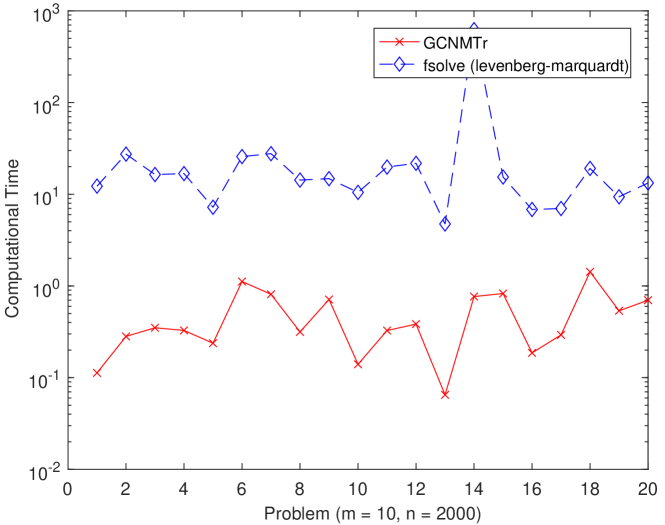
Figure 1: The computational time of GCNMTr and fsolve for the underdetermined problems with $m=10,\,n=2000$.

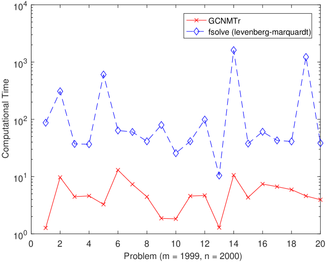
Figure 2: The computational time of GCNMTr and fsolve for the underdetermined problems with $m=1999,\;n=2000$.

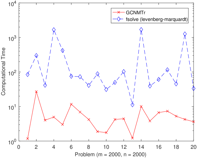
Figure 3: The computational time of GCNMTr and fsolve for the determined problems with $m=2000,\;n=2000$.

The numerical results are arranged in Tables 1-3. NJ stands for the number of the Jacobian evaluations required for convergence in Tables 1-3. The computational time of GCNMTr and fsolve is illustrated by Figures 1-3. From Tables 1-3, we find that GCNMTr performs well for those test problems, and the levenberg-marquardt method (fsolve) fails to solve some problems.

Furthermore, from Figures 1-3 and Tables 1-3, we also find that GCNMTr is faster than the Levenberg-Marquardt method (fsolve) and the computational time of GCNMTr is about $1/8$ to $1/50$ of that of fsolve. One of the reasons is that GCNMTr does not need to update the Jacobian matrix $J_{k}$ and decompose it when it performs well. This strategy can save much computational time, in comparison to that of the updating the Jacobian matrix $J(x_{k})$ at every iteration for the traditional Levenberg-Marquardt method. The other reason is that fsolve uses the QR decomposition to solve the linear system (64), which requires $2n^{2}(2n/3+m)$ flops (p. 264, GV2013 ). However, GCNMTr uses the QR decomposition to solve the linear systems of equation (21), which only requires $2m^{2}(n-m/3)$ flops and about the half of that of fsolve.

Table 1: Numerical results of GCNMTr and fsolve for the underdetermined problems with $m=10,\;n=2000$.

Problems	GCNMTr		fsolve.m (levenberg-marquardt)
	NJ (Iteration, time$/s$)	$||F(x^{it})||_{\infty}$	Iteration (time$/s$)	$||F(x^{it})||_{\infty}$
1. Trid Function SB2013 (m = 10, n = 2000)	2 (14, 0.1127$s$)	1.6495E-08	5 (12.2854$s$)	2.8635E-11
2. Grewank Function SB2013 (m = 10, n=2000)	2 (11, 0.2816$s$)	5.6776E-07	10 (27.3960$s$)	5.0238E-16
3. Dixon Price Function SB2013 (m = 10, n = 2000)	5 (20, 0.3500$s$)	5.2291E-07	7 (16.4054$s$)	1.2434E-14
4. Rosenbrock Function MGH1981 (m = 10, n = 2000)	5 (24, 0.3274$s$)	4.1377E-07	7 (16.7926$s$)	6.1729E-11
5. Trigonometric Function MGH1981 (m = 10, n = 2000)	2 (11, 0.2375$s$)	1.4611E-07	3 (7.2162$s$)	8.5720E-12
6. Singular Broyden Function Luksan1994 (m = 10, n = 2000)	19 (35, 1.1180$s$)	4.3241E-07	12 (25.7608$s$)	0.0213 (failed)
7. Extended Powell Singular Function MGH1981 (m = 10, n = 2000)	10 (25, 0.8116$s$)	7.7570E-07	12 (27.7080$s$)	7.5422E-07
8. Tridiagonal System Function Luksan1994 (m = 10, n = 2000)	6 (20, 0.3157$s$)	4.8995E-07	8 (14.2731$s$)	2.2095E-08
9. Discrete Boundary-Value Function Luksan1994 (m = 10, n = 2000)	2 (13, 0.7122$s$)	6.8392E-07	5 (14.7863$s$)	7.5662E-13
10. Broyden Tridiagonal Function Luksan1994 (m = 10, n = 2000)	2 (15, 0.1398$s$)	1.9205E-07	5 (10.4810$s$)	1.5421E-10
11. Extended Wood Function Andrei2008 (m = 10, n = 2000)	6 (22, 0.3264$s$)	7.0474E-08	8 (19.7991$s$)	5.8124E-09
12. Extended Cliff Function Andrei2008 (m = 10, n = 2000)	6 (21, 0.3839$s$)	9.6747E-07	10 (21.7415$s$)	1.5466E-08
13. Extended Hiebert Function Andrei2008 (m = 10, n = 2000)	2 (13, 0.0650$s$)	1.4634E-08	2 (4.7399$s$)	5.0164E-12
14. Extended Maratos Function Andrei2008 (m = 10, n = 2000)	16 (37, 0.7660$s$)	7.4567E-07	199 (623.0145$s$)	0.1757 (failed)
15. Extended Psc1 Function Andrei2008 (m = 10, n = 2000)	5 (20, 0.8269$s$)	6.1415E-07	7 (15.4128$s$)	2.3426E-14
16. Extended Quadratic Penalty QP 1 Function Andrei2008 (m = 10, n = 2000)	2 (18, 0.1863$s$)	6.1455E-08	3 (6.8182$s$)	1.1303E-14
17. Extended Quadratic Penalty QP 2 Function Andrei2008 (m = 10, n = 2000)	2 (20, 0.2924$s$)	5.7408E-07	3 (6.9848$s$)	6.5782E-12
18. Extended TET Function Andrei2008 (m = 10, n = 2000)	7 (22, 1.4268$s$)	2.1258E-07	8 (19.1292$s$)	7.8478E-11
19. EG2 Function Andrei2008 (m = 10, n = 2000)	2 (16, 0.5359$s$)	6.3057E-08	4 (9.3791$s$)	6.1195E-13
20. Extended BD1 Function Andrei2008 (m = 10, n = 2000)	5 (19, 0.6993$s$)	1.1822E-07	6 (13.2805$s$)	1.4782E-08

Table 2: Numerical results of GCNMTr and fsolve for the underdetermined problems with $m=1999,\;n=2000$.

Problems	GCNMTr		fsolve.m (levenberg-marquardt)
	NJ (Iteration, time$/s$)	$||F(x^{it})||_{\infty}$	Iteration (time$/s$)	$||F(x^{it})||_{\infty}$
1. Trid Function SB2013 (m = 1999, n = 2000)	2 (14, 1.2698$s$)	1.6764E-08	14 (87.1366$s$)	2.5611E-09
2. Grewank Function SB2013 (m = 1999, n=2000)	12 (29, 9.7008$s$)	2.1524E-07	36 (308.7068$s$)	4.9506E-16
3. Dixon Price Function SB2013 (m = 1999, n = 2000)	6 (21, 4.4584$s$)	8.6397E-09	7 (37.1861$s$)	1.5824E-08
4. Rosenbrock Function MGH1981 (m = 1999, n = 2000)	6 (22, 4.5985$s$)	4.8484E-09	7 (36.7351$s$)	1.2921E-09
5. Trigonometric Function MGH1981 (m = 1999, n = 2000)	13 (30, 3.2750$s$)	3.1687E-07	70 (605.1742$s$)	2.2600e-05 (failed)
6. Singular Broyden Function Luksan1994 (m = 1999, n = 2000)	19 (35, 13.0141$s$)	5.2082E-07	12 (63.8643$s$)	0.0213 (failed)
7. Extended Powell Singular Function MGH1981 (m = 1999, n = 2000)	10 (25, 7.3242$s$)	7.7570E-07	11 (60.1272$s$)	7.5422E-07
8. Tridiagonal System Function Luksan1994 (m = 1999, n = 2000)	6 (20, 4.4418$s$)	5.3380E-07	8 (41.2931$s$)	1.6009E-14
9. Discrete Boundary-Value Function Luksan1994 (m = 1999, n = 2000)	2 (13, 1.8657$s$)	1.8195E-07	6 (79.6152$s$)	1.5319E-12
10. Broyden Tridiagonal Function Luksan1994 (m = 1999, n = 2000)	2 (15, 1.8283$s$)	3.0495E-07	5 (25.6165$s$)	1.4704E-10
11. Extended Wood Function Andrei2008 (m = 1999, n = 2000)	6 (22, 4.5732$s$)	7.0474E-08	8 (41.4228$s$)	5.8341E-09
12. Extended Cliff Function Andrei2008 (m = 1999, n = 2000)	6 (21, 4.6795$s$)	9.6747E-07	10 (98.8046$s$)	1.5507E-08
13. Extended Hiebert Function Andrei2008 (m = 1999, n = 2000)	2 (16, 1.2882$s$)	1.4830E-08	2 (10.4330$s$)	8.0231E-10
14. Extended Maratos Function Andrei2008 (m = 1999, n = 2000)	16 (37, 10.5885$s$)	7.4568E-07	199 (1612.5726$s$)	0.1757 (failed)
15. Extended Psc1 Function Andrei2008 (m = 1999, n = 2000)	5 (22, 4.3262$s$)	2.0538E-07	7 (37.6980$s$)	8.4970E-13
16. Extended Quadratic Penalty QP 1 Function Andrei2008 (m = 1999, n = 2000)	10 (26, 7.4105$s$)	2.2681E-07	11 (60.6542$s$)	1.5642E-04 (failed)
17. Extended Quadratic Penalty QP 2 Function Andrei2008 (m = 1999, n = 2000)	7 (32, 6.6672$s$)	4.6757E-08	8 (42.7976$s$)	1.2390E-05 (failed)
18. Extended TET Function Andrei2008 (m = 1999, n = 2000)	7 (24, 5.9189$s$)	1.4731E-07	8 (41.0473$s$)	7.8525E-11
19. EG2 Function Andrei2008 (m = 1999, n = 2000)	5 (22, 4.5872$s$)	3.1190E-08	153 (1225.0636$s$)	1.3816E-10
20. Extended BD1 Function Andrei2008 (m = 1999, n = 2000)	5 (19, 3.9460$s$)	7.2238E-07	7 (38.3996$s$)	1.0549E-14

Table 3: Numerical results of GCNMTr and fsolve for the determined problems with $m=2000,\;n=2000$.

Problems	GCNMTr		fsolve.m (levenberg-marquardt)
	NJ (Iteration, time$/s$)	$||F(x^{it})||_{\infty}$	Iteration (time$/s$)	$||F(x^{it})||_{\infty}$
1. Trid Function SB2013 (m = 2000, n = 2000)	2 (14, 1.1696$s$)	1.6764E-08	15 (84.5851$s$)	2.3283E-10
2. Grewank Function SB2013 (m = 2000, n=2000)	37 (64, 26.9887$s$)	3.5969E-07	36 (299.4471$s$)	4.9853E-16
3. Dixon Price Function SB2013 (m = 2000, n = 2000)	6 (21, 4.0241$s$)	8.6667E-09	7 (41.3923$s$)	1.5895E-08
4. Rosenbrock Function MGH1981 (m = 2000, n = 2000)	6 (22, 4.9494$s$)	6.5022E-08	199 (1671.5553$s$)	0.0043 (failed)
5. Trigonometric Function MGH1981 (m = 2000, n = 2000)	4 (13, 3.0073$s$)	3.4463E-07	44 (420.8693$s$)	2.2750E-05 (failed)
6. Singular Broyden Function Luksan1994 (m = 2000, n = 2000)	19 (35, 11.6583$s$)	5.5066E-07	12 (75.0792$s$)	0.0226 (failed)
7. Extended Powell Singular Function MGH1981 (m = 2000, n = 2000)	10 (25, 6.9210$s$)	7.7570E-07	12 (73.0282$s$)	7.5422E-07
8. Tridiagonal System Function Luksan1994 (m = 2000, n = 2000)	6 (20, 4.2114$s$)	1.7450E-07	7 (40.8813$s$)	1.8865E-11
9. Discrete Boundary-Value Function Luksan1994 (m = 2000, n = 2000)	2 (13, 1.8843$s$)	6.8400E-07	13 (88.6350$s$)	1.0325E-11
10. Broyden Tridiagonal Function Luksan1994 (m = 2000, n = 2000)	3 (15, 1.7556$s$)	8.1420E-07	5 (31.1220$s$)	1.3323E-15
11. Extended Wood Function Andrei2008 (m = 2000, n = 2000)	6 (22, 4.2280$s$)	7.0474E-08	8 (49.8806$s$)	5.8341E-09
12. Extended Cliff Function Andrei2008 (m = 2000, n = 2000)	6 (21, 4.4264$s$)	9.6747E-07	10 (102.9089$s$)	1.5507E-08
13. Extended Hiebert Function Andrei2008 (m = 2000, n = 2000)	2 (16, 1.2165$s$)	1.4634E-08	2 (11.2343$s$)	5.0164E-12
14. Extended Maratos Function Andrei2008 (m = 2000, n = 2000)	16 (37, 10.0705$s$)	7.4567E-07	199 (1692.7199$s$)	0.1757 (failed)
15. Extended Psc1 Function Andrei2008 (m = 2000, n = 2000)	5 (20, 3.8124$s$)	6.1415E-07	7 (39.2547$s$)	2.4758E-14
16. Extended Quadratic Penalty QP 1 Function Andrei2008 (m = 2000, n = 2000)	11 (27, 6.6775$s$)	7.5538E-08	11 (60.9623$s$)	5.2307E-04 (failed)
17. Extended Quadratic Penalty QP 2 Function Andrei2008 (m = 2000, n = 2000)	10 (32, 7.3550$s$)	3.4402E-09	10 (115.7199$s$)	0.2043 (failed)
18. Extended TET Function Andrei2008 (m = 2000, n = 2000)	7 (22, 5.2577$s$)	2.1258E-07	8 (45.2060$s$)	7.8525E-11
19. EG2 Function Andrei2008 (m = 2000, n = 2000)	5 (22, 4.2430$s$)	3.1007E-08	153 (1264.3533$s$)	1.2457E-10
20. Extended BD1 Function Andrei2008 (m = 2000, n = 2000)	5 (19, 3.6184$s$)	1.1822E-07	6 (33.3613$s$)	1.4783E-08

5 Conclusions

In this article, we consider the generalized continuation Newton method with the trust-region updating strategy and the new updating technique of the Jacobian matrix for the underdetermined system (GCNMTr). For some large-scale underdetermined and determined problems, numerical results show that GCNMTr is more robust and faster than the traditional optimization method such as the Levenberg-Marquardt method (the subroutine fsolve.m of the MATLAB R2020a environment). The computational time of GCNMTr is about $1/8$ to $1/50$ of that of fsolve. We also analyze the global convergence and the local superlinear convergence of the new method under the standard assumptions. From our point of view, the generalized continuation Newton method (Algorithm 1) can be regarded as an alternative workhorse for the nonlinear equations and we will extend it to the constrained nonlinear programming problems.

Declarations

Funding: This work was supported in part by Grant 61876199 from National Natural Science Foundation of China, and Grant YJCB2011003HI from the Innovation Research Program of Huawei Technologies Co., Ltd..

Conflicts of interest/Competing interests: Not applicable.

Availability of data and material (data transparency): If it is requested, we will provide the test data.

Code availability (software application or custom code): If it is requested, we will provide the code.

References

• (1) Andrei, N.: An unconstrained optimization test functions collection, Environ. Sci. Technol. 10, 6552-6558 (2008)
• (2) Allgower, E.L., Georg, K.: Introduction to Numerical Continuation Methods, SIAM, Philadelphia (2003)
• (3) Ascher, U.M., Petzold, L.R.: Computer Methods for Ordinary Differential Equations and Differential-Algebraic Equations, SIAM, Philadelphia (1998)
• (4) Axelsson, O., Sysala, S.: Continuation Newton methods, Comput. Math. Appl. 70, 2621-2637 (2015)
• (5) Branin, F.H.: Widely convergent method for finding multiple solutions of simultaneous nonlinear equations, IBM J. Res. Dev. 16, 504-521 (1972)
• (6) Brenan, K.E., Campbell, S.L., L. R. Petzold, L.R.: Numerical solution of initial-value problems in differential-algebraic equations, SIAM, Philadelphia (1996)
• (7) Conn, A.R., Gould, N., Toint, Ph.L: Trust-Region Methods, SIAM, Philadelphia (2000)
• (8) Davidenko, D.F.: On a new method of numerical solution of systems of nonlinear equations (in Russian), Dokl. Akad. Nauk SSSR 88, 601-602 (1953)
• (9) Deuflhard, P.: Newton Methods for Nonlinear Problems: Affine Invariance and Adaptive Algorithms, Springer, Berlin (2004)
• (10) Deuflhard, P., Pesch, H.J., Rentrop, P.: A modified continuation method for the numerical solution of nonlinear two-point boundary value problems by shooting techniques, Numer. Math. 26, 327-343 (1975)
• (11) Dennis, J.E, Schnabel, R.B: Numerical Methods for Unconstrained Optimization and Nonlinear Equations, SIAM, Philadelphia (1996)
• (12) Doedel, E.J.: Lecture notes in numerical analysis of nonlinear equations, in: Krauskopf, B., Osinga, H.M., Galán-Vioque, J. (Eds.): Numerical Continuation Methods for Dynamical Systems, pp. 1-50, Springer, Berlin (2007)
• (13) Fan, J.-Y., Yuan, Y.-X.: On the quadratic convergence of the Levenberg–Marquardt method, Comput. 74, 23-39 (2005)
• (14) Gottlieb, S., Shu, C.W.: Total variation diminishing Runge-Kutta schemes, Math. Comput. 67, 73-85 (1998)
• (15) Gottlieb, S., Shu, C.W., Tadmor, E.: Strong stability preserving high order time discretization methods, SIAM Rev. 43, 89-112 (2001)
• (16) Golub, G.H, Van Loan, C.F.: Matrix Computation (4th ed.), The John Hopkins University Press, Baltimore (2013)
• (17) Griewank, A.: On solving nonlinear equations with simple singularities or nearly singular solutions, SIAM Rev. 27, 537-563 (1985)
• (18) Hairer, E., Lubich, C. and Wanner, G.: Geometric Numerical Integration: Structure-Preserving Algorithms for Ordinary Differential Equations, 2nd ed., Springer, Berlin (2006)
• (19) Hairer, E., Wanner, G.: Solving Ordinary Differential Equations II, Stiff and Differential-Algebraic Problems (2nd ed.), Springer, Berlin (1996)
• (20) Hiebert, K.L.: An evaluation of mathematical software that solves systems of nonlinear equations, ACM Trans. Math. Softw. 8, 5-20 (1982)
• (21) Higham, D.J.: Trust region algorithms and timestep selection, SIAM J. Numer. Anal. 37, 194-210 (1999)
• (22) Izmailov, A.F., Solodov, M.V. and Uskov, E.I.: A globally convergent Levenberg–Marquardt method for equality-constrained optimization, Comput. Optim. Appl. 72, 215-239 (2019)
• (23) Kalaba, R.F., Zagustin, E., Holbrow, W., Huss, R.: A modification of Davidenko’s method for nonlinear systems, Comput. Math. Appl. 3, 315-319 (1977)
• (24) Kelley, C.T., Keyes, D.E.: Convergence analysis of pseudo-transient continuation, SIAM J. Numer. Anal. 35, 508-523 (1998)
• (25) Kelley, C.T.: Solving Nonlinear Equations with Newton’s Method, SIAM, Philadelphia (2003)
• (26) Kelley, C.T.: Numerical methods for nonlinear equations, Acta Numer. 27, 207-287 (2018)
• (27) Liu, D.G., Fei and J. G.: Digital Simulation Algorithms for Dynamic Systems (in Chinese), Science Press, Beijing (2000)
• (28) Levenberg, K.: A method for the solution of certain problems in least squares, Q. Appl. Math. 2, 164-168 (1944)
• (29) Liao, S.J.: Homotopy Analysis Method in Nonlinear Differential Equations, Springer, Berlin (2012)
• (30) Lukšan, L.: Inexact trust region method for large sparse systems of nonlinear equations, J. Optim. Theory Appl. 81, 569-590 (1994)
• (31) Luo, X.-L., Liu, D.G.: Real-time simulation algorithms for computing differential-algebraic equation, Chinese J. Numer. Math. Appl. 22, 71-80 (2001)
• (32) Luo, X.-L.: Singly diagonally implicit Runge-Kutta methods combining line search techniques for unconstrained optimization, J. Comput. Math. 23, 153-164 (2005)
• (33) Luo, X.-L.: A trajectory-following method for solving the steady state of chemical reaction rate equations, J. Theor. Comput. Chem. 8, 1025-1044 (2009)
• (34) Luo, X.-L.: A second-order pseudo-transient method for steady-state problems, Appl. Math. Comput. 216, 1752-1762 (2010)
• (35) Luo, X.-L., Liao, L.-Z., Tam, H.-W., Convergence analysis of the Levenberg-Marquardt method, Optim. Methds Softw. 22, 659-678 (2007)
• (36) Luo, X.-L., Lv, J.-H. and Sun, G.: Continuation methods with the trusty time-stepping scheme for linearly constrained optimization with noisy data, Optim. Eng., published online at http://doi.org/10.1007/s11081-020-09590-z, 1-32, 2021
• (37) Luo, X.-L., Xiao, H., Lv, J.-H.: Continuation Newton methods with the residual trust-region time-stepping scheme for nonlinear equations, Numer. Algorithms, published online at http://doi.org/10.1007/s11075-021-01112-x, 1-25, 2021.
• (38) Luo, X.-L., Yao, Y.-Y.: Primal-dual path-following methods and the trust-region strategy for linear programming with noisy data, J. Comput. Math., published online at http://doi.org/10.4208/jcm.2101-m2020-0173, 1-21, or available at http://arxiv.org/abs/2006.07568, 2021
• (39) Luo, X.-L., Xiao, H., Lv, J.-H., Zhang, S.: Explicit pseudo-transient continuation and the trust-region updating strategy for unconstrained optimization, Appl. Numer. Math. 165, 290-302 (2021)
• (40) MATLAB v9.8.0 (R2020a), The MathWorks Inc., http://www.mathworks.com, 2020
• (41) Marquardt, D.: An algorithm for least-squares estimation of nonlinear parameters, SIAM J. Appl. Math. 11, 431-441 (1963)
• (42) Moré, J.J.: The Levenberg-Marquardt algorithm: Implementation and theory, in: Watson G.A. (eds.): Numerical Analysis, Lecture Notes in Mathematics, vol. 630, pp. 105-116, Springer, Berlin (1978)
• (43) Moré, J.J., Garbow, B.S., Hillstrom, K.E.: Testing unconstrained optimization software, ACM Trans. Math. Softw. 7, 17-41 (1981)
• (44) Nocedal, J., Wright, S.J.: Numerical Optimization, Springer, Berlin (1999)
• (45) Ortega, J.M., Rheinboldt, W.C.: Iteration Solution of Nonlinear Equations in Several Variables, SIAM, Philadelphia (2000)
• (46) Powell, M.J.D.: Convergence properties of a class of minimization algorithms, in: Mangasarian, O.L., Meyer, R.R., Robinson, S.M. (eds.): Nonlinear Programming 2, pp. 1-27, Academic Press, New York (1975)
• (47) Qian, J., Andrew, A. L., Chu, D. L. and Tan, R. C. E.: Methods for solving underdetermined systems, Numer. Linear Algebra Appl. 25, e2127 (2017)
• (48) Surjanovic, S., Bingham, D.: Virtual library of simulation experiments: Test functions and datasets, available at http://www.sfu.ca/~ssurjano, January 2020
• (49) Shampine, L.F., Gladwell, I., Thompson, S.: Solving ODEs with MATLAB, Cambridge University Press, Cambridge (2003)
• (50) Sun, W.Y., Yuan, Y.X.: Optimization Theory and Methods: Nonlinear Programming, Springer, New York (2006)
• (51) Tanabe, K.: Continuous Newton-Raphson method for solving an underdetermined system of nonlinear equations, Nonlinear Anal. 3, 495-503 (1979)
• (52) Watson, L.T., Sosonkina, M., Melville, R.C., Morgan, A.P., Walker, H.F.: HOMPACK90: A suite of fortran 90 codes for globally convergent homotopy algorithms, ACM Trans. Math. Softw. 23, 514-549 (1997)
• (53) Yamashita, N., Fukushima, M.: On the rate of convergence of the Levenberg-Marquardt method, Comput. 15 [Suppl.], 239-249 (2001)
• (54) Yuan, Y.X.: Trust region algorithms for nonlinear equations, Information 1, 7-20 (1998)
• (55) Yuan, Y.X.: Recent advances in trust region algorithms, Math. Program. 151, 249-281 (2015)