Scalable Online Recurrent Learning Using
Columnar Neural Networks

Abstract

Structural credit assignment for recurrent learning is challenging. An algorithm called RTRL can compute gradients for recurrent networks online but is computationally intractable for large networks. Alternatives, such as BPTT, are not online. In this work, we propose a credit-assignment algorithm — Master-User — that approximates the gradients for recurrent learning in real-time using $O(n)$ operations and memory per-step. Our method builds on the idea that for modular recurrent networks, composed of columns with scalar states, it is sufficient for a parameter to only track its influence on the state of its column. We empirically show that as long as connections between columns are sparse, our method approximates the true gradient well. In the special case when there are no connections between columns, the $O(n)$ gradient estimate is exact. We demonstrate the utility of the approach for both recurrent state learning and meta-learning by comparing the estimated gradient to the true gradient on a synthetic test-bed.

1 Introduction

Structural credit-assignment — identifying how to change network parameters to improve predictions — is an essential component of learning in neural networks. Effective structural credit-assignment requires tracking the influence of parameters on future predictions. A parameter can influence a prediction in the future in two primary ways. First, for recurrent networks (RNNs), a parameter can influence the internal state of the network which, in turn, can affect a prediction made many steps in the future. Second, if the network is learning online, a parameter can influence the learning updates. These learning updates, in turn, influence predictions made in the future. Structural credit-assignment through recurrent states is called recurrent state learning, whereas through the learning updates is called meta-learning (Schmidhuber, 1987; Bengio et al., 1990; and Sutton, 1992).

Back-Propagation Through Time (BPTT) (Werbos, 1988; Robinson and Fallside, 1987) is a popular algorithm for gradient-based structural credit-assignment in RNNs. BPTT extends the back-propagation algorithm for feed-forward networks — independently proposed by Werbos (1974) and Rumelhart et al. (1986) — to RNNs by storing network activations from prior steps, and repeatedly applying the chain-rule starting from the output of the network and ending at the activations at the beginning of the sequence. BPTT is unsuitable for online learning as it requires memory proportional to the length of the sequence. Moreover, it delays gradient computation until the end of the sequence. For online learning, this sequence can be never-ending or arbitrarily long.

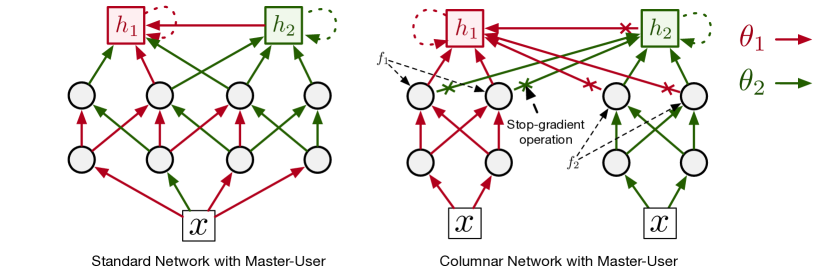
Figure 1: We can divide $\theta$ into $\{\theta_{1},\theta_{2}\}$ randomly, or in columns. The red parameters are $\theta_{1}$ and green $\theta_{2}$. Our goal is to estimate $\frac{\partial h_{i}}{\partial\theta_{i}}$ for $i=1$ and $2$. For the network on the left, this would require two backward passes — one starting from $h_{1}$ and one from $h_{2}$. For the Columnar network on the right, on the other hand, we can back-propagate gradients starting from the sum $h_{1}+h_{2}$ and stop the flow of gradients from parameters connecting the features from one column to the feature of others. We show the stop-gradient operations with ’$\times$’ on the arrows. The stop-gradient operations allows us to compute $\frac{\partial h_{i}}{\partial\theta_{i}}$ exactly for $i=1$ and $2$ in a single backward pass. Organizing parameters in columns is key to estimating the required gradient in a single pass.

RTRL — an alternative to BPTT — was proposed by Williams and Zipser (1989). RTRL relies on forward-mode differentiation — using chain-rule to compute gradients in the direction of time — to compute gradients recursively. Unlike BPTT, RTRL does not delay gradient-computation until the final step. The memory requirement of RTRL also does not depend on the sequence length. As a result, it is a better candidate for real-time online learning. Unfortunately, RTRL requires maintaining the Jacobian $\frac{\partial h(t)}{\partial\theta}$ at every step, which requires $O(|h||\theta|)$ memory, where $|h|$ is the size of state of the network and $|\theta|$ is the number of total parameters. The Jacobian is recursively updated by applying chain rule as:

$$\frac{\partial h(t+1)}{\partial\theta}=\frac{\partial h(t+1)}{\partial\theta(t+1)}+\frac{\partial h(t+1)}{\partial h(t)}\frac{\partial h(t)}{\partial\theta},$$

which requires $O(|h|^{2}|\theta|)$ operations and scales poorly to large networks.

A promising direction to scale gradient-based credit-assignment to large networks is to approximate the gradient. Elman (1990) proposed to ignore the influence of parameters on future predictions completely for training RNNs. This resulted in a scalable but biased algorithm. Williams and Peng (1990) proposed a more general algorithm called Truncated BPTT (T-BPTT). T-BPTT tracks the influence of all parameters on predictions made up to $k$ steps in the future. T-BPTT is implemented by limiting the BPTT computation to last $k$ activations and works well for a range of problems (Mikolov et al., 2009, 2010; Sutskever, 2013 and Kapturowski et al., 2018). Its main limitation is that the resultant gradient is blind to long-range dependencies. Mujika et al. (2018) showed that on a simple copy task, T-BPTT failed to learn dependencies beyond the truncation window. Tallec et al. (2017) demonstrated T-BPTT can even diverge when a parameter has a negative long-term effect on a target and a positive short-term effect.

RTRL can also be approximated to reduce its computational overhead. Ollivier et al. (2015) and Tallec et al. (2017) proposed NoBacktrack and UORO. Both of these algorithms provide stochastic unbiased estimates of the gradient and scale well. However, their estimates have high variance and require extremely small step sizes for effective learning. Cooijmans and Martens (2019) and Menick et al. (2021) showed that, for practical problems, UORO does not perform well due to its high variance compared to other biased approximations. Menick et al. (2021) proposed an approximation to RTRL called SnAp-$k$. SnAp-$k$ tracks the influence of a parameter on a state only if the parameter can influence the state within $k$ steps. It first identifies parameters whose influence on a state is zero for $k$ steps and then assumes the future influence to be zero as well. For the remaining parameters, it tracks their influence on all future predictions. T-BPTT, on the other hand, ignores the influence of all parameters on all predictions made after $k$ steps. This makes SnAp-k less biased than T-BPTT with a truncation window of $k$. SnAp-1 can be computationally efficient but introduces significant bias. SnAp-$k$ for $k>1$ reduces bias but can be as expensive as RTRL for dense RNNs. Menick et al. (2021) further proposed using sparse connections as a way to make SnAp more scalable. Connection sparsity reduces the number of parameters that can influence a state within $k$ steps Menick et al. (2021) showed that for highly sparse networks, SnAp-$k$ reduces the computational requirement of RTRL by over 95% while keeping bias in check. One limitation of their work is that they do not provide a scalable method to identify parameters that would not influence a state within $k$ steps. Instead, they run the RNN for $k$ steps and look at the full Jacobian $\frac{\partial h(t)}{\partial\theta}$ to determine these parameters. For large networks, computing this Jacobian even once is not possible. Moreover, because they induce sparsity randomly in their networks, the resultant sparsity in the Jacobian is not structured and is not amenable to efficiency gains using existing hardware. Finally, SnAp does not scale well when used in conjunction with deep feature extractors. If internal states operate on a shared representation computed with a deep network with parameters $\theta$, even SnAp-1 could require $O(|\theta||h|)$ memory and $O(|\theta||h|^{2})$ operations per-step. Our goal is to design an algorithm that requires $O(|\theta|)$ memory and operations.

We propose an algorithm — called Master-User — and a recurrent network architecture — called Columnar Neural Networks (Col-NNs). Master-User requires $O(|h||\theta|)$ operations and $O(|\theta|)$ memory per-step for credit assignment in existing recurrent networks. When combined with Col-NNs, the time complexity of Master-User reduces to $O(|\theta|)$. The central idea behind Col-NNs is that recurrent learning can be made more efficient by modularizing the network. For a special class of Col-NNs, Master-User can even estimate the exact gradients in $O(|\theta|)$ time.

2 Problem Formulation

Let $\theta\in\mathbb{R}^{p}$ be the parameters of a recurrent network and $h(t)\in~{}\mathbb{R}^{n}$ be the hidden state at time $t$. The network combines the state $h(t)$ linearly using $w(t)\in\mathbb{R}^{n}$ to make a prediction $y(t)$ as:

$$y(t)=\sum_{i=1}^{n}w_{i}(t)h_{i}(t)$$ (1)

Let $y^{*}(t)$ be the target at time $t$. Then the error in the prediction is given by:

$$\delta(t)=y^{*}(t)-y(t).$$

Our goal is to minimize the error

$$\mathcal{L}(t)=\frac{1}{2}\delta^{2}(t).$$

The goal of a gradient-based credit-assignment algorithm can be formalized as estimating or approximating credit given by:

$$G(t) =\frac{\partial\mathcal{L}(t)}{\partial\theta}$$ (2)

Here $\theta$ is not indexed by $t$ because we want to estimate the impact of $\theta$ at all prior time-steps on the current prediction. Since computing this exact gradient using BPTT or RTRL is expensive, we aim to approximate it. We propose an algorithm called Master-User.

3 The Master-User Algorithm

The central idea behind Master-User is to divide the parameters of an RNN into $n$ disjoint groups — $\theta=\{\theta_{1},\theta_{2},\cdots,\theta_{n}\}$ — and assign every group to a scalar hidden state. Let $\theta_{i}$ be assigned to $h_{i}$. Then, Master-User estimates the influence of $\theta_{i}$ on $h_{i}(t)$ by approximating $\frac{\partial h_{i}(t)}{\partial\theta_{i}}$ online. For $i\neq j$, it ignores the influence of $\theta_{i}$ on $h_{j}(t)$ and treats $\frac{\partial h_{j}(t)}{\partial\theta_{i}}=0$ . We call $h_{i}$ the master state for $\theta_{i}$ — it can pass gradients to $\theta_{i}$ for assigning credit — whereas $h_{j}$ is the user state — it can only use features generated by $\theta_{i}$, but cannot change those features by assigning credit. To keep track of influence of $\theta_{i}$ on $h_{i}$, The trace of the gradient $\frac{\partial h_{i}(t)}{\partial\theta_{i}}$ can be computed recursively as:

$$\frac{\partial h_{i}(t)}{\partial\theta_{i}}=\frac{\partial h_{i}(t)}{\partial\theta_{i}(t)}+\frac{\partial h_{i}(t)}{\partial h(t-1)}\frac{\partial h(t-1)}{\partial\theta_{i}}.$$ (3)

The update involves $\frac{\partial h(t-1)}{\partial\theta_{i}}$ — a Jacobian of size $|h|\times|\theta_{i}|$. Computing this Jacobian is expensive so Master-User approximates the update by ignoring the influence of $\theta_{i}$ on $h_{i}$ through states $h_{j}$ as:

$$\frac{\partial h_{i}(t)}{\partial\theta_{i}}\approx\frac{\partial h_{i}(t)}{\partial\theta_{i}(t)}+\frac{\partial h_{i}(t)}{\partial h_{i}(t-1)}\frac{\partial h_{i}(t-1)}{\partial\theta_{i}},$$ (4)

where $\frac{\partial h_{i}(t)}{\partial\theta_{i}(t)}$ is the gradient of $h_{i}(t)$ that takes into account the influence of $\theta_{i}$ only at time $t$. The terms $\frac{\partial h_{i}(t)}{\partial\theta_{i}(t)}$ and $\frac{\partial h_{i}(t)}{\partial h_{i}(t-1)}$ can be computed in $O(|\theta|)$ operations using the back-propagation algorithm . The product $\frac{\partial h_{i}(t)}{\partial h_{i}(t-1)}\frac{\partial h_{i}(t-1)}{\partial\theta_{i}}$ and the summation in Equation 4 take $O(|\theta_{i}|)$ operations. Equation 4 has to be repeated for each hidden state, making the overall complexity $O(|h||\theta|)$ which falls short of our goal of an order $O(|\theta|)$ algorithm.

Applying Master-User to standard RNNs is unlikely to work well. Master-User completely ignores the influence of $\theta_{i}$ on $h_{j}$ and only approximates the influence of $\theta_{i}$ on $h_{i}$. In the next section, we introduce an architecture called Columnar Neural Networks (Col-NNs) for which the approximations made by Master-User are sensible. Moreover, Master-User can exploit the structure in Col-NNs to scale linearly with number of parameters.

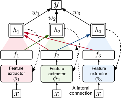
Figure 2: A three column Col-NN. The red region and red arrows represent the parameters for the first column. Arrows connecting a column with the state of a different column — such as the red arrow from $f_{3}$ to $h_{1}$ — are called lateral connections. Lateral connections allow a column to use features learned by other columns, but they also introduce error in the estimate of the gradient. When there are no lateral connections, exact gradient for a Col-NN can be computed in $O(|\theta|)$ time.

4 Columnar Neural Networks

Master-User divides the parameter into $n$ disjoint groups, but does not specify how these groups are constructed. Parameters in $\theta_{i}$ can be spread all over the network, or assigned randomly. Columnar Neural Networks (Col-NNs) impose further structure on these groups by organizing them into $n$ columns. Every column has an associated feature extractor. The feature extractor for the $i$th column, $C_{\phi_{i}}$, is parameterized by $\phi_{i}$. It takes as input $x(t)$ and $h_{i}(t-1)$ and outputs a feature vector $f_{i}(t)\in\mathbb{R}^{k}$ i.e.,

$$f_{i}(t)=C_{\phi_{i}}(x(t),h_{i}(t-1))$$

Hidden state $h_{i}$ is updated as:

$$h_{i}(t)=\mathcal{R}_{u_{i}}(f_{1}(t),f_{2}(t),\cdots,f_{n}(t),h(t-1))$$

where $\mathcal{R}_{u_{i}}$ is parameterized by $u_{i}$ and defines a recursive relationship between $h_{i}(t)$ and $h_{i}(t-1)$. The set of parameters $\{u_{i},\phi_{i}\}$ constitute the group $\theta_{i}$. $\mathcal{R}_{u_{i}}$ can be used to implement existing recurrent architectures, such as an LSTM or GRU cell. An abstracted view of a Col-NN is shown in Figure 2.

Col-NN restricts the architecture of the feature extractor, but provides a key benefit from an optimization point of view — it can reduce the overhead of Master-User from $O(|h||\theta|)$ to $O(|\theta|)$. This is possible because for a Col-NN, the set of gradients $\{\frac{\partial h_{i}(t)}{\partial\theta_{i}(t)}\}_{i=1}^{n}$ — required by Equation 4 — can be computed by using back-propagation only once.

4.1 $O(|\theta|)$ Implementation of Master-User for Col-NNs

In Section 3, we noted that we need a separate application of back-propagation for computing $\frac{\partial h_{i}(t}{\partial\theta_{i}(t)}$ for each $i$. For Col-NNs, it is possible to compute $\frac{\partial h_{i}(t}{\partial\theta_{i}(t)}$ for all $i$ with a single application of back-propagation.

We modify back-propagation by restricting the backward flow of gradient from state $h_{j}$ to features $f_{i}$, as shown in Figure 1. We then compute the gradient of the sum of the states $\frac{\partial(\sum_{k=1}^{n}h_{k}(t))}{\partial\theta(t)}$; the resultant gradient is $\{\frac{\partial h_{i}(t)}{\partial\theta_{i}(t)}\}_{i=1}^{n}$. To see why, note that the gradient of the sum is equal to sum of gradients i.e.,

$$\frac{\partial\left(\sum_{k=1}^{n}h_{k}(t)\right)}{\partial\theta(t)} =\sum_{k=1}^{n}\frac{\partial h_{k}(t)}{\partial\theta(t)}.$$ (5)

If we can remove gradients $\frac{\partial h_{j}(t)}{\partial\theta_{i}(t)}$ for $j\neq i$ in Equation 5 from the computation graph, back-propagation w.r.t the sum will give us $\frac{\partial(\sum_{k=1}^{n}h_{k}(t))}{\partial\theta(t)}$. To remove the gradients $\frac{\partial h_{j}(t)}{\partial\theta_{i}(t)}$ for $j\neq i$, we modify back-propagation so that it ignores the flow of gradient from $f_{j}$ to $\phi_{i}$ as shown in Figure 1 (Right). Because $h_{j}(t)$ can only be influenced by $\theta_{i}(t)$ through $f_{i}(t)$, ignoring gradient from $h_{j}(t)$ to $f_{i}(t)$ is all we need to ignore $\frac{\partial h_{j}(t)}{\partial\theta_{i}(t)}$ for $j\neq i$. Applying this modified back-propagation algorithm gives us $\{\frac{\partial h_{i}(t)}{\partial\theta_{i}(t)}\}_{i=1}^{n}$ for all parameters in the same number of operations as a single application of back-propagation. The same reasoning can be used to show that $\{\frac{\partial h_{i}(t)}{\partial h_{i}(t-1)}\}_{i=1}^{n}$ can be computed in a single backward pass. These two terms, when plugged into Equation 4, give us $\{\frac{\partial h_{i}(t)}{\partial\theta_{i}}\}_{i=1}^{n}$ in $O(|\theta|)$ operations.

5 Credit-Assignment in Recurrent Learning

Master-User provides the gradient estimate for all parameters w.r.t their master state. We use this estimate to approximate $G(t)$ introduced in Equation 2 as follows:

$$G(t) =\frac{\partial\mathcal{L}(t)}{\partial\theta_{i}}$$

$$=\frac{\partial\delta^{2}(t)}{2\partial\theta_{i}}$$

$$=\delta(t)\frac{\partial\delta(t)}{\partial\theta_{i}}$$

$$=\delta(t)\frac{\partial(y^{*}(t)-\sum_{j=1}^{n}w_{j}(t)h_{j}(t))}{\partial\theta_{i}}$$

$$=-\delta(t)\sum_{j=1}^{n}w_{j}(t)\frac{\partial h_{j}(t)}{\partial\theta_{i}}$$ (6)

Assuming $$\frac{\partial h_{j}(t)}{\partial\theta_{i}}=0 i\neq j$$ when

$$\approx-\delta(t)w_{i}(t)\frac{\partial h_{i}(t)}{\partial\theta_{i}}.$$ (7)

All terms in Equation 7 can be computed in $O(|\theta|)$ time and memory for Col-NN, as discussed in the previous section.

5.1 Making Sense of the Approximations

Credit-assignment using Master-User required two approximations. First, we approximated:

$$\frac{\partial h_{i}(t)}{\partial h_{j}(t-1)}\frac{\partial h_{j}(t-1)}{\partial\theta_{i}}\approx 0\text{ when }i\neq j$$ (8)

to simplify Equation 3 to Equation 4. Second, we approximated:

$$\frac{\partial h_{j}(t)}{\partial\theta_{i}}\approx 0\text{ when }i\neq j$$ (9)

to simplify Equation 6 to Equation 7. If the approximation in Equation 9 holds, then the approximation in Equation 8 follows.

A Col-NN provides an easy way to make $\frac{\partial h_{j}(t)}{\partial\theta_{i}}\approx 0$. In a Col-NN, $\theta_{i}$ can only influence $h_{j}(t)$ through the feature $f_{i}(t)$. Let the connections from $f_{i}(t)$ to $h_{j}(t)$ for $i\neq j$ be called lateral connections as shown in Figure 2. Then, removing all lateral connections would make the approximation in Equation 9 to hold exactly, allowing us to compute the true gradient in $O(|\theta|)$ time. A downside of removing all lateral connections is that $h_{i}(t)$ can no longer use features generated by $\theta_{j}$, or information stored in $h_{j}(t-1)$, to update itself. Instead of removing lateral connections entirely, we propose to make lateral connections sparse to reduce the influence of $\theta_{i}$ on $h_{j}$.

5.2 Evaluating Quality of the Gradient Estimate

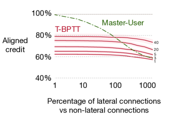
Figure 3: Quality of the approximation as a function of lateral connectivity. When number of lateral connections are low compared to non-lateral connections, the gradient estimate of Master-User is highly aligned with the true gradient. As lateral connections increase, the approximation gets worse. T-BPTT’s estimate has significantly higher error for Col-NNs with sparse lateral connections even when the truncation window — 40 — is almost equal to the sequence length — 50. All curves are averaged over 100 random seems, and the confidence intervals are one standard error.

We compare the $O(n)$ gradient estimate of Master-User in a Col-NN to the true gradient computed using BPTT on a synthetic benchmark.

5.2.1 Synthetic Benchmark

We randomly generate input and target sequences. Input $x(t)$ is a vector of length fifty. Each element of the input vector is uniformly sampled from the set $\{0,1\}$. Target $y^{*}(t)$ is uniformly sampled from the range $(-50,50)$. Random targets result in high error and large gradients, which is useful for testing the quality of the gradient estimate.

5.2.2 Network Architecture

Each column of the Col-NN implements a 2-layer fully connected network with 50 features in each layer and ReLU activations (Glorot et al., 2011). The output of each column is a feature of length 50. We use a total of 20 columns. The parameters of our network are initialized using Xavier Initialization (Glorot and Bengio, 2010) to ensure a high flow of gradient. The recurrence function, $h_{j}(t)=\mathcal{R}_{u_{j}}(f_{1}(t),\cdots,f_{n}(t),h_{j}(t-1))$ is defined as:

$$h_{i}(t)=h_{i}(t-1)+\sigma_{g}(\sum_{j=1}^{n}U^{T}_{ij}f_{j}(t)+R^{T}_{i}h(t-1))$$ (10)

where $U_{i}$ is a matrix with dimensions $|h|\times|f_{j}|$, $R_{i}$ is a vector of length $|h|$ and $\sigma_{g}$ is the $tanh$ function. We use recurrence defined in Equation 10 instead of popular architectures, like LSTM (Hochreiter and Schmidhuber, 1997) or GRU (Cho et al., 2014), because untrained LSTM or GRU networks initialized using popular initialization techniques decay the information in recurrent cell rapidly, removing long-term dependencies. Equation 10, on the other hand, does not decay the old state at all resulting in long-term dependencies between parameters and predictions. Our recurrent function is a poor choice for practical problems, but is useful for evaluating the accuracy of credit-assignment algorithms for capturing long-term dependencies. For more details on the decay rate in untrained LSTM and GRU networks, and results with GRU networks, see Appendix A.

5.2.3 Controlling Sparsity in Lateral Connections

We make the weight vector $U_{ij}$ for $i\neq j$ sparse by masking weights at random to be zero. This reduces the influence of $f_{j}$ on $h_{i}(t)$ for . Let $m$ be the number of unmasked weights in $U_{ij}$ for all $j\neq i$ and $n$ be the number of weights in $U_{ii}$ that connect $f_{i}(t)$ to $h_{i}(t)$. Then, percentage of lateral connections vs non-lateral connections is defined as $s=\frac{m}{n}$. When $s=100\%$, the number of lateral connections is the same as non-lateral connections whereas $s=1000\%$ implies there are ten times more lateral connections than non-lateral connections. For a visual depiction of lateral connections, see Figure 2.

5.2.4 Results

We evaluate the accuracy of our gradient estimate by comparing it to the true gradient $\sum_{i=1}^{50}\frac{\partial\mathcal{L}(i)}{\partial\theta}$ and report the results in Figure 3. We report the percentage of estimated gradient that points in the same direction as the true gradient. Our choice is motivated by the observation that as long as the approximate gradient estimate points in the same direction as the true gradient, we can expect the parameters to move in the right direction. We include T-BPTT as a baseline with truncation windows of 1, 3, 5, 20, and 40. When lateral connections are few, the estimate of the gradient using Master-User is highly aligned with the true gradient. The misalignment increases as $s$ increases. This matches our expectations — when $s$ is small, the approximation $\frac{\partial h_{i}(t)}{\theta_{j}}\approx 0$ holds better. The gradient estimate is exact when there are no lateral connections. Sparsity has little effect on the gradient estimate of T-BPTT. The estimate of T-BPTT improves with the truncation window, but is worse than the estimate of Master-User for sparse Col-NNs. Even T-BPTT with a truncation window of 40 performs worse than Master-User when lateral connections are few. Note that the sequence length is only 50, and truncation window of 40 is very close to full BPTT. We repeated the experiment for a range of Col-NNs configurations and found the results to be consistent across different settings. For details of all the configurations, hyper-parameters, and results using the GRU cell, see Appendix B.

6 Credit-Assignment in Meta-learning

Similar to recurrent state learning, meta-learning also requires structural credit assignment. Both BPTT and RTRL have been used successfully used for meta-learning.

Finn et al. (2017) and Li et al. (2017) independently proposed using BPTT for learning through a stochastic gradient descent (SGD) update in a deep neural network. Javed and White (2019) showed that T-BPTT can be used for meta-learning through long correlated sequences for learning without forgetting.

RTRL has also been used for meta-learning. Sutton (1992) showed that it can be used to learn the step-sizes for a linear predictor. Veeriah et al. (2017) extended Sutton’s analysis by using it to approximate the meta-gradients for a one layer neural network. Applying RTRL to deep-learning based meta-learning methods is not tractable. MAML (Finn et al. 2017) — a meta-learning algorithm that updates all parameters online at each learning step — would require $O(|\theta|^{2})$ memory and $O(|\theta|^{3})$ operations per-step to recursively compute the meta-gradient. An alternative to MAML is the OML architecture — independently proposed by Javed and White (2019), and Bengio et al. (2020). The OML architecture updates only the parameters in the final prediction layers — $W$ — of the network at every step and updates the remaining parameters — $\theta$ — using the meta-gradient. Computing meta-gradients for the OML architecture using RTRL requires $O(|W||\theta|)$ memory and $O(|W^{2}||\theta|)$ operations per-step. For $|W|<|\theta|$, this is already significantly more tractable than the $O(|\theta|^{3})$ operations required by MAML. However, the memory and operations still do not scale linearly with the size of the network.

We show that the OML architecture with a linear prediction layer can be combined with Col-NNs to approximate the meta-gradients online using $O(|\theta|)$ operations and memory. The key to our approximation, once again, is to exploit the modular structure of Col-NNs to remove insignificant gradient terms.

6.1 Scalable Meta-learning using Col-NNs

Once again we want to estimate $\frac{\partial L(t)}{\partial\theta_{i}}$, but with a key difference — the network is updating the prediction parameters $w$ at every step. The parameters $w(t)$ linearly combine the state $h(t)$ for making predictions, as described in Equation 1. The weights $w_{i}(t)$ are updated as:

$$w_{i}(t+1) =w_{i}(t)-\alpha_{i}\frac{\partial\mathcal{L}(t)}{\partial w_{i}(t)}$$

$$=w_{i}(t)-\alpha_{i}\delta(t)\frac{\partial(y^{*}(t)-y(t))}{\partial w_{i}(t)}$$

$$=w_{i}(t)+\alpha_{i}\delta(t)\frac{\partial\sum_{j=1}^{n}w_{j}(t)h_{j}(t)}{\partial w_{i}(t)}$$

$$=w_{i}(t)+\alpha_{i}\delta(t)h_{i}(t)$$ (11)

where $a_{i}$ is the step-size parameter. Equation 11 is the standard least mean squares (LMS) learning rule. The gradients for the loss $\mathcal{L}(t)$ w.r.t the parameters $\theta$ through the LMS learning rule can be computed as:

$$\frac{\partial\mathcal{L}(t)}{\partial\theta_{i}} =\frac{\partial\delta^{2}(t)}{2\partial\theta_{i}}$$

$$\frac{\partial\mathcal{L}(t)}{\partial\theta_{i}} =\delta(t)\frac{\partial\delta(t)}{\partial\theta_{i}}$$ (12)

$$=\delta(t)\frac{\partial(y^{*}(t)-\sum_{k=1}^{n}w_{k}(t)h_{k}(t))}{\partial\theta_{i}}$$

$$=-\delta(t)\sum_{k=1}^{n}\frac{\partial(w_{k}(t)h_{k}(t))}{\partial\theta_{i}}$$

$$\frac{\partial w_{k}(t)}{\partial\theta_{i}}\neq 0$$ for an online learning network.

Using product rule

$$=-\delta(t)\sum_{k=1}^{n}\left(w_{k}(t)\frac{\partial h_{k}(t)}{\partial\theta_{i}}+h_{k}(t)\frac{\partial w_{k}(t)}{\partial\theta_{i}}\right)$$ (13)

Using the Master-User approximation,

$$\frac{\partial(h_{k}(t)))}{\partial\theta_{i}}\approx 0\text{ when }i\neq k\implies$$

$$\approx-\delta(t)\left(w_{i}(t)\frac{\partial h_{i}(t)}{\partial\theta_{i}}+\sum_{k=1}^{n}h_{k}(t)\frac{\partial w_{k}(t)}{\partial\theta_{i}}\right)$$ (14)

For Col-NN with sparse lateral connections,

$$\theta_{i}\text{ only indirectly influences }w_{k}\text{ when }i\neq k$$

$$\implies\frac{\partial(w_{k}(t)))}{\partial\theta_{i}}\approx 0\implies$$ (15)

$$\frac{\partial\mathcal{L}(t)}{\partial\theta_{i}} \approx-\delta(t)\left(w_{i}(t)\frac{\partial h_{i}(t)}{\partial\theta_{i}}+h_{i}(t)\frac{\partial w_{i}(t)}{\partial\theta_{i}}\right)$$ (16)

The approximation used in Equation 15 is similar to the one proposed by Veeriah et al. (2017) for one layer networks. In deep networks, this is a poor approximation in the general case. We later show that the modular structure of Col-NNs is key for making this approximation work for multi-layer networks.

We can compute $\frac{\partial h_{i}(t)}{\partial\theta_{i}}$ in Equation 16 in $O(|\theta|)$ as explained in the Sections 4.1. $\frac{\partial w_{i}(t)}{\partial\theta_{i}}$ requires more work. Let:

$$TW_{\theta_{i}}(t) \vcentcolon=\frac{\partial w_{i}(t)}{\partial\theta_{i}}$$ (By definition) (17)

$$TW_{\theta_{i}}(0) \vcentcolon=0$$ (By definition) (18)

Then:

$$TW_{\theta_{i}}(t+1) =\frac{\partial w_{i}(t+1)}{\partial\theta_{i}}$$

Using LMS learning rule from Equation 11

$$TW_{\theta_{i}}(t+1) =\frac{\partial(w_{i}(t)+\alpha_{i}\delta(t)h_{i}(t))}{\partial\theta_{i}}$$

Using Definition 17

$$=TW_{\theta_{i}}(t)+\frac{\partial}{\partial\theta_{i}}(\alpha_{i}\delta(t)h_{i}(t))$$

Using product rule

$$=TW_{\theta_{i}}(t)+\alpha_{i}\delta(t)\frac{\partial h_{i}(t)}{\partial\theta_{i}}$$

$$+\alpha_{i}h_{i}(t)\frac{\partial\delta(t)}{\partial\theta_{i}}$$ (19)

From Equation 12 and 16, we can infer:

$$\frac{\partial\delta(t)}{\partial\theta_{i}} \approx-w_{i}(t)\frac{\partial h_{i}(t)}{\partial\theta_{i}}-h_{i}(t)\frac{\partial w_{i}(t)}{\partial\theta_{i}}$$

$$\approx-w_{i}(t)\frac{\partial h_{i}(t)}{\partial\theta_{i}}-h_{i}(t)TW_{i}(t)$$ (20)

All the terms in Equation 19 and 20 can be computed using $O(|\theta|)$ operations, allowing us to compute gradients through the LMS learning rule efficiently. Note that meta-learning requires an additional trace per parameter — the $TW_{\theta}$ matrix.

6.2 Making Sense of the Approximations

The meta-gradient computation introduces two additional approximations to the gradient. First, it simplifies Equation 13 to Equation 14 by assuming:

$$\frac{\partial h_{k}(t)}{\partial\theta_{i}}\approx 0\text{ when }i\neq k$$

and second, it simplifies Equation 14 to Equation 15 by assuming:

$$\frac{\partial w_{k}(t)}{\partial\theta_{i}}\approx 0\text{ when }i\neq k$$ (21)

The first approximation is the same as one used to estimate the gradient through the recurrent states. We know that for Col-NNs with sparse lateral connections, it is a reasonable approximation. For the second approximation, we note from Equation 11 that $\theta_{i}$ can influence the learning update to $w_{k}(t)$ by influencing two terms. First, it can influence $h_{k}(t)$ and second, it can influence the overall error $\delta(t)$. We know $\frac{\partial h_{k}(t)}{\partial\theta_{i}}\approx 0$ for Col-NNs with sparse lateral connections. Veeriah et al. (2017) and Sutton (1992) empirically showed that the indirect effect of a parameter on the weight update through change in error is insignificant. This makes sense as $\frac{\partial\delta(t-1)}{\partial\theta_{i}}\frac{\partial w_{k}(t)}{\partial\delta(t-1)}$ is a product of two small numbers.

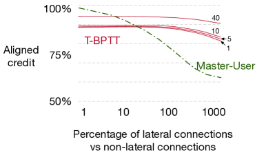
Figure 4: Quality of the approximation of the meta-gradient as a function of lateral connectivity. When number of lateral connections are low compared to non-lateral connections, the gradient estimate of Master-User for meta-learning is aligned with the true gradient. As lateral connections increase, the approximation gets worse. T-BPTT performs noticeably worse than Col-NN when lateral connections are sparse. The truncation window for T-BPTT is written at the end of each curve. All curves are averaged over 100 random seems, and the confidence intervals are one standard error.

Figure 5: Ignoring the meta-gradient through the LMS update significantly impacts the accuracy of the estimate of the gradient. Even for a network with no lateral connections, less than 90% of the gradients are unaligned when we ignore the meta-gradient. In many real-time recurrent systems, the last layer prediction weights are updated online and the meta-gradient is ignored. Our results suggest that doing so can be detrimental for effective credit-assignment.

6.3 Evaluating Quality of the Gradient Estimate

6.3.1 Experiment Setup

We use the test-bed described in Section 21 to answer two questions. First, we evaluate how well Master-User approximates the meta-gradient in isolation. We then test the importance of meta-gradients for estimating the true gradient of an online learning recurrent network. To answer the first question, we note that the error in the estimate of the meta-gradient can either be due to approximations made when computing gradients through the LMS rule or due to the approximations made when estimating gradient of the recurrent states. To disentangle the two sources of error, we modify the state update to be:

$$h_{i}(t)=\sigma_{g}(\sum_{j=1}^{n}U^{T}_{ij}f_{j}(t))$$ (22)

to remove the recurrence. We use the same network architecture as Section 21. At every step, we update the weights $w$ using the LMS learning rule. We use a step-size of $1e^{-2}$ for each $w_{i}$ and compare the estimated gradient to the true gradient computed using BPTT. We use T-BPTT with truncation windows of 1, 5, 10, and 40 as baselines. For results for other choices of step-sizes and architectures, see Appendix B.

6.3.2 Results

We report the results in Figure 4. Master-User performs better than T-BPTT with any truncation window when Col-NNs has sparse lateral connections. For a Col-NN with no lateral connections, the gradient estimate of Master-User is close to exact demonstrating that the effect of $\theta_{i}$ on $w_{k}(t)$ through error $\delta(t-1)$ is indeed insignificant as speculated in Section 6.2. We note that the benefit of Master-User for estimating the meta-gradient is less pronounced than the benefit for the recurrent gradient reported previously in Figure 3. This could be either because for meta-gradients, long-term dependencies are not as important or because our test-bed does not capture the long-term dependencies that can otherwise emerge in meta-learning. Nonetheless, for up to 10% ratio of lateral connection vs non-lateral connections, Master-User performs better than T-BPTT with a truncation window of 10 for estimating the meta-gradients.

Lastly, we investigate the importance of the meta-gradient to the overall gradient in an online learning recurrent network. We run Col-NNs on our test-bed twice, updating the final prediction weights $w$ at each step using the LMS rule with a step-size of $1e^{-2}$. In the first run, we estimate the gradient using Equation 16. This estimate takes into account gradient through both the recurrent state and the LMS weight update. In the second run, we ignore the gradient through the LMS weight update. This can be done by setting $\frac{\partial w_{i}(t))}{\partial\theta_{i}}$ to zero in Equation 16. We report the results in Figure 5. We find that ignoring the meta-gradient significantly impacts the accuracy of the overall gradient. Even for a columnar network with no lateral connections, less than $90\%$ of the gradients are aligned if we ignore the meta-gradient completely. We also report the average MAE between the estimates and the true gradient and find that ignoring the meta-gradient increases the error by $50\%$.

7 Conclusion and Discussion

Scalable online recurrent learning is crucial for applying machine learning knowledge to real-world problems. In this work, we proposed one such method to achieve scalable online learning. Our method approximates the gradient for recurrent learning using $O(n)$ operations and memory. The approximations made by our method are interpretable. Additionally, the accuracy of the approximation can be controlled by controlling a tunable parameter. We also unify recurrent state learning and meta-learning and show that the same ideas can be applied to scale both. Finally, our method can be combined with arbitrary deep feature-extractors, opening the possibility of combining deep learning with online recurrent learning. There are key questions that our work leaves unanswered. Do modularized networks have limited capacity compared to fully connected networks? How does the accuracy of the gradient estimate changes as the network learn online? Can we increase the number of lateral connections overtime when features in columns have stabilized? We leave these questions for future work.

.

Appendix A Information Decay in Randomly Initialized LSTM and GRU Networks

In the main text, we reported results using an RNN with recurrence defined by Equation 10. Our recurrence relationship simply adds to the hidden state to get the new state. This results in a challenging benchmark for gradient-estimation in which parameter can influence a target many steps in the future. A randomly initialized LSTM or GRU cell, on the other hand, is not guaranteed to have long-range dependencies. To show this empirically, we measure how many steps can information propagate in untrained LSTM and GRU networks. We set the internal states of the networks to be a vector of one, and update the state for 20 steps using a zero vector as input. Using a zero input vector prevents addition of any new information in the state, and allows us to measure the decay of initial value of the state.

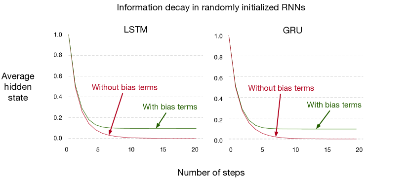
Figure 6: Information decay in randomly initialized LSTM (left) and GRU (right) cells. We initialize the hidden state for both to be 1, and then run each for 20 steps. Both networks see a zero vector as input. The hidden state for both LSTM and GRU without bias terms decays to zero quickly showing that these architectures, when untrained, do not involve long-range dependencies. This makes them a poor candidate for comparing gradient approximation methods. When the bias terms are not zero, the hidden state converges to a non-zero constant due to the bias term.

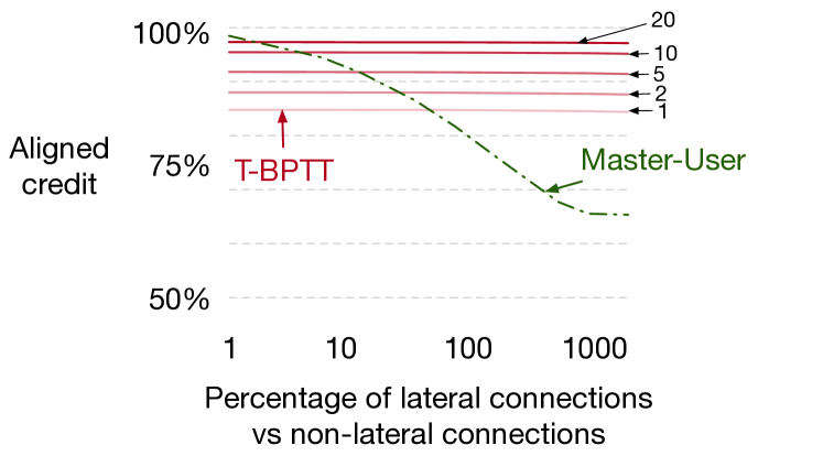
Figure 7: Quality of the approximation as a function of lateral connectivity for a GRU based RNN. The value of truncation window for T-BPTT is indicated by numbers at the end of each curve. A randomly initialized GRU decays information in the hidden state rapidly. This improves the performance of T-BPTT with small truncation windows. However, the good performance of T-BPTT is expected to deteriorate once the GRU call has learned longer-range dependencies.

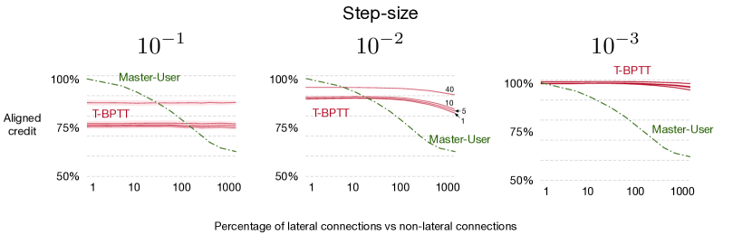
Figure 8: Effect of step-size parameter on gradient approximation for T-BPTT and Master-User. When step-size is large, T-BPTT is a poor approximation to the true gradient. Even a truncation window of 40 — almost equal to the sequence length 50 — is not sufficient to approximate the meta-gradient well. The error introduced by Master-User, on the other hand, does not vary with step-size. This makes Master-User a promising algorithm for meta-learning with large step-sizes.

We initialize the LSTM and GRU parameters by uniformly sampling the weights between $(-\sqrt{k},\sqrt{k})$ where $k$ is $\frac{1}{\textit{hidden units}}$. This is the default initialization used by Pytorch (Paszkeet al., 2019). We report the results for LSTM and GRU networks with and without the bias terms for $k=50$ in Figure 6. Other values of $k$ give similar results. From Figure 6, we see that the information in LSTM and GRU cells decays rapidly. Without any bias terms, the hidden state is close to zero with-in just 5 steps and approaches zero in 10 steps. This suggests that for randomly initialized GRU and LSTM cells, T-BPTT with a small truncation window would perform well.

The rapid decay in LSTM and GRU cells is not surprising. The value of the forget gate for untrained LSTM and GRU cells initialized using popular initialization methods is $\approx 0.5$ which makes information decay exponentially. Note that trained LSTM and GRU cells do not suffer from this — their forget gate can output 1 resulting in no decay of information.

A.1 Results with GRU Networks

We run experiment described in Section 21 using randomly initialized GRU cells and report the results in Figure 7. Because randomly initialized GRUs decay information quickly, T-BPTT with small truncation window performs significantly better than it does in Figure 3. Note that the good performance of T-BPTT can only be expected to hold on the untrained GRU RNN. Once the GRU cell starts learning, the decay rate of information can reduce — depending on the learning signal — and the gradient approximation of T-BPTT could deteriorate. Col-NNs trained with Master-User do no suffer from this — their error in gradient-estimation stays low for sparse lateral connections even when there are long-range dependencies, as shown in Figure 3.

Appendix B Experiment details

B.1 Hyper-parameters

The key parameters in our experiments are number of columns (C), number of units in each layer of the column (W), and the step-size (SS). We tried C = 5, 10, 20, 50, 100; W = 5, 10, 20, 50, 100; and SS = $10^{-1},10^{-2},10^{-3}$. SS is a parameter only for the meta-learning experiment. C and W result in 25 combinations for the RNN experiments and wherease C, W, and SS result in 75 combinations for the meta-learning experiments. We did 100 runs for each configuration resulting in a total of 10,000 runs. We found that changing C and W does not change the results qualitatively and the results are similar to those reported in Figure 3. The SS parameter does influence the result noticeably and we report those in the next section.

B.2 Effect of Step-size on Approximation of the Meta-gradient

We report the effect of changing SS for a network with C = 20 and W = 50 in Figure 8. When SS is large, T-BPTT performs worse. This makes sense — a large step-size increases the influence of parameters on future predictions and T-BPTT with small truncation window is a poor approximation to the gradient. For smaller step-sizes, the effect of parameters on future predictions is minuscule and even T-BPTT with a truncation window of 1 is a good approximation. The error in approximation due to Master-User is independent of the step-size. This makes Master-User ideal for meta-learning with large step-sizes.

B.3 Compute Resources and Reproducibility

We used two 48 core CPU servers for all the experiments. All experiments in the paper can be reproduced in less than 5 hours using the two servers. We ran each configuration using 100 random seeds. Running each configuration only once can be done on a personal computer in a few hours. We provide anonymized code for reproducing the experiments at https://github.com/khurramjaved96/columnar_networks.

References

Paszke, Adam, et al. ”Pytorch: An imperative style, high-performance deep learning library.” arXiv preprint arXiv:1912.01703 (2019).