Word Embedding Techniques for Malware Evolution Detection

Abstract

Malware detection is a critical aspect of information security. One difficulty that arises is that malware often evolves over time. To maintain effective malware detection, it is necessary to determine when malware evolution has occurred so that appropriate countermeasures can be taken. We perform a variety of experiments aimed at detecting points in time where a malware family has likely evolved, and we consider secondary tests designed to confirm that evolution has actually occurred. Several malware families are analyzed, each of which includes a number of samples collected over an extended period of time. Our experiments indicate that improved results are obtained using feature engineering based on word embedding techniques. All of our experiments are based on machine learning models, and hence our evolution detection strategies require minimal human intervention and can easily be automated.

1 Introduction

Malware is malicious software that causes disruption in normal activity, allows access to unapproved resources, gathers private data of users, or performs other improper activity [1]. Developing measures to detect malware is a critical aspect of information security.

Malware often evolves due to changing goals of malware developers, advances in detection, and so on [3]. This evolution can occur through a wide variety of modifications to the code. It is essential to detect and analyze malware evolution so that appropriate measures can be taken to maintain and improve the effectiveness of detection techniques [2].

An obvious technique for analyzing malware evolution consists of reverse engineering a large number of samples over an extended period of time, which is a highly labor-intensive process. Other approaches to malware evolution include graph pruning techniques [7] and analysis of PE file features using support vector machines (SVM) [29]. This latter research shows considerable promise, and has the advantage of being fully automated, with no reverse engineering or other time-consuming analysis required. Our proposed research can be viewed as an extension of—and improvement on—the groundbreaking work in [29].

We consider several experiments that are designed to detect points in time where a malware family has likely evolved significantly. We then perform further experiments to confirm that such evolution has actually occurred. All of our experiments have been conducted using a significant number of malware families, most of which include a large number of samples collected over an extended period of time. Furthermore, all or our experiments are based on machine learning, and hence fully automatable.

For a given malware family, we first separate the available samples based on windows of time. We have extracted opcode sequences from every sample and we use these opcodes as features for detecting malware evolution. We experiment with a variety of feature engineering techniques, and in each case we train linear SVMs over sliding windows of time. The SVM weights of these models are compared based on a $\chi^{2}$ distance measure, which enables us to detect changes in the SVM models over time. A point in time where a spike is observed in the $\chi^{2}$ graph shows a substantial change in SVM models—which indicates a possible evolutionary branch in the malware family under consideration. To confirm that such evolution has actually occurred, we train hidden Markov models (HMM) on either side of a significant spike in the $\chi^{2}$ graph. If a clear distinction between these HMMs is observed, it serves as confirmation that significant evolution has been detected. The primary objective of this research is to implement and analyze different variants of this proposed malware evolution detection technique.

The remainder of this paper is organized as follows. In Section 2 we discuss relevant related work in the area of malware evolution. Section 3 provides an overview of the dataset that we use, as well as brief introductions to the various machine learning models and techniques that we use in this research. We present our experimental results in Section 4. The paper concludes with Section 5, where we also outline possible avenues for future work.

2 Related Work

Relative to the vast malware research literature, comparatively little has been done in the area of malware evolution. In this section, we provide a selective review of research related to malware evolution.

The malware evolution research in [7] is based on large and diverse malware dataset that spans nearly two decades. This work focuses on inheritance properties of malware, and the technique is based on graph pruning. The authors claim that many specific traits of various families in their dataset have been “inherited” from other families. However, it is not entirely clear that these “inherited” traits are actually inherited, as opposed to having been developed independently. In addition, the graph-based analysis in [7] requires “extensive manual investigation,” which is in stark contrast to the automated techniques that are considered in this paper.

The authors of [9] extract a variety of features from Android malware samples and determine trends based on standard software quality metrics. These results are compared to a similar analysis of trends in Android non-malware, or goodware. This work shows that the trends in Android malware and goodware are fairly similar, indicating that the “improvement” in this type of malware has followed a similar path as that of goodware.

The paper [24] is focused on detecting new malware variants, which is closely related to an evolution problem. The authors considered malware variants that would typically defeat machine learning based detectors. Their approach relies an an extensive feature set and employs semi-supervised learning. In comparison, the approach in this paper relies entirely on unsupervised techniques, and we are able to detect less drastic code modifications.

The work in [4] is nominally focused on malware taxonomy. However, this work also provides insight into malware evolution, in the form of “genealogical trajectories.” The work relies on a variety of features and uses support vector machines (SVM) for classification.

We note in passing that machine learning models are trained on features. Thus, extracting appropriate features from a dataset is a crucial step in any malware analysis technique that is based on machine learning. We can broadly classify features as static and dynamic—features that can be obtained without executing the code are said to be static, while those that require code execution or emulation are known as dynamic. In general, static features are more efficient to collect, whereas dynamic features can be more informative and are typically more robust [5].

The author in [29] use static PE file features of malware samples as the basis for their malware evolution research. Based on these feature, linear SVMs are trained over various time windows and the resulting model weights are compared using a $\chi^{2}$ distance. A spike in the $\chi^{2}$ distance graph is shown to be indicative of an evolutionary change in a malware family. Note that this approach is easily automated, with no reverse engineering required.

The research presented in this paper extends and expands on the work in [29]. As in [29], we use SVMs together with $\chi^{2}$ distance as a means of detecting evolutionary change. We make several important contributions that greatly increase the utility of this basic approach. The novelty of our work includes the use of more sensitive static features—we use opcodes as compared to derived PE file features—and we employ various feature engineering techniques. In addition, we develop an HMM-based secondary test to verify the putative evolutionary changes obtained from the SVM together with a $\chi^{2}$ distance.

3 Implementation

In this section, we give a broad summary of the malware families that comprise the dataset used in the research. We also discuss the features and machine learning techniques used in our experiments. These features and techniques forms the basis of our evolutionary experiments in Section 4.

3.1 Dataset

A malware family represents a collection of samples that have major traits in common. Over time, successful malware families will tend to evolve, as malware writers develop new features and find different applications for the code base.

The research in this paper is based of a malware dataset consisting of Windows portable executable (PE) files. From a large dataset, we have extracted 11,037 samples belonging to 15 distinct malware families. Table 1 lists these malware families and the number of samples per family that we use in our experiments.

Table 1: Number of samples used in experiments

Family	Samples	Years
Adload	791	2009–2011
BHO	1116	2007–2011
Bifrose	577	2009–2011
CeeInject	742	2009–2012
DelfInject	401	2009–2012
Dorkbot	222	2005–2012
Hupigon	449	2009–2011
IRCBot	59	2009–2012
Obfuscator	670	2004–2017
Rbot	127	2001–2012
VBInject	2331	2009–2018
Vobfus	700	2009–2011
Winwebsec	1511	2008–2012
Zbot	835	2009–2012
Zegost	506	2008–2011
Total	11,037	—

Our Winwebsec and Zbot malware samples were acquired from the Malicia dataset [23], while the remaining thirteen families were extracted from a vast malware dataset that was collected as part of the work reported in [8]. This latter dataset is greater than half a terabyte in size and contains on the order of 500,000 malware executables. Our datasets is available from the authors upon request.

Most of the malware families that were chosen for this research have a substantial number of samples available over an extended time period. The smaller families (e.g., IRCBot and Rbot) were chosen to test the our analysis techniques in cases where the training data is severely limited.

As a pre-processing step, we have organized all the malware samples in each family according to their creation date. During this initial data wrangling phase, any sample having an altered compilation or creation date was discarded.

Next, we briefly discuss each of the malware families in our dataset. Note that these families represent a wide variety of types of malware, including Trojan, worm, adware, backdoor, and so on.

Bifrose

is a backdoor Trojan that allows an attacker to connect to a remote IP using a random port number. Some variants of Bifrose have the capability to hide files and processes from the user. Bifrose enables an attacker to view system information, retrieve passwords, or execute files by gaining remote control of an infected system [22].

CeeInject

serves to shielding nefarious activity from detection. For example, CeeInject can obfuscate a bitcoin mining client, which might be installed on a system to mine bitcoins without the user’s knowledge [13].

DelfInject

is a worm that enters a system from a file passed by other malware, or as a file downloaded accidentally by a client when visiting malignant sites. DelfInject drops itself onto the system using an arbitrary document name (e.g., xpdsae.exe) and alters the relevant registry entry so that it runs at each system start. The malware then injects code into svchost.exe so that it can create a connection with specific servers and download files [14].

Dorkbot

is a worm that steals user names and passwords by tracking online activities. It blocks security update websites and can launch denial of service (DoS) attacks. Dorkbot is spread via instant messaging applications, social networks, and flash drives [21].

Hotbar

is an adware program that may be unintentionally downloaded by a user from a malicious website. Being adware, Hotbar displays advertisements as the user browses the web [11].

Hupigon

is a family of backdoor Trojans. This malware opens a backdoor server enabling other remote computers to control a compromised system [12].

Obfuscator

hides its purpose through obfuscation. The underlying malware can have virtually any payload [18].

Rbot

is a backdoor Trojan that enables an attacker to control an infected computer using an IRC channel. It then spreads to other computers by scanning for network shares and exploiting vulnerabilities in the system. Rbot includes many advanced features and it has been used to launch DoS attacks [10].

VBInject

primarily serves to disguise other malware. VBInject is a packaged malware, i.e., malware that utilizes techniques of encryption and compression to obscure its contents. This makes it difficult to recognize malware that it is concealing. VBInject was first seen in 2009 and appeared again in 2010 [15].

Vobfus

is a malware family that downloads other malware onto a user’s computer. It uses the Windows autorun feature to spread to other devices such as flash drives. Vobfus makes long lasting changes to the device configuration that cannot be restored simply by removing the malware from the system [16].

Winwebsec

is a Trojan that presents itself as an antivirus software. It shows misleading messages to the users stating that the device has been infected and attempts to persuade the user to pay to remove these non-existent threats [17].

Zbot

is a Trojan that attempts to steal confidential information from a compromised computer. It explicitly targets system data, online sensitive data, and banking information, and it can also be easily modified to accumulate other kinds of data. The Trojan itself is generally disseminated through drive-by downloads and spam campaigns. Zbot was originally discovered in January 2010 [19].

Zegost

is a backdoor Trojan that injects itself into svchost.exe, thus allowing an attacker to execute files on the compromised system [20].

3.2 Feature Extraction

Mnemonic opcodes are machine-level language instructions that specify a particular operation that is to be performed [26]. For this research, our dataset consists of malware samples in the form of portable executable (PE) files. The primary feature that we consider are opcode sequences extracted from these executable files. We have also segregated the malware samples in each family according to their creation date.

3.3 Classification Techniques

In this section we will provide an overview of each machine learning technique that we employ in this research. Additional pointers to the literature are provided.

3.3.1 Support Vector Machines

Support vector machines (SVM) are one of the most popular classes of machine learning techniques. An SVM attempts to find a separating hyper-plane between two labeled classes of data [27]. By utilizing the so-called “kernel trick”, an SVM can map the input data to a high-dimensional space where the additional space can afford a greater opportunity to find a separating hyperplane. The “trick” of the kernel trick is that this mapping does not result in any significant increase in the work factor.

A linear SVM assigns a well-defined weight to each feature in the training vector. These weights specify the relative importance that the SVM places on each feature which can serve as a useful when ranking the importance of features. In our experiments, we rely heavily on this aspect of linear SVMs.

Analogos to [29], in our experiments, we define the two classes of an SVM as follows. All the samples within the most recent one-year time window are class “$+1$”, while all samples from the current month are defined as class “$-1$”. For example, in Table 2 we give three consecutive time windows, along with the time frames corresponding to the two classes in each case.

Table 2: Sliding time window example

Time Window	Class $+1$	Class $-1$
Jan. 2011–Jan. 2012	Jan. 2011–Dec. 2011	Jan. 2012
Feb. 2011–Feb. 2012	Feb. 2011–Jan. 2012	Feb. 2012
Mar. 2011–Mar. 2012	Mar. 2011–Feb. 2012	Mar. 2012

3.3.2 $\chi^{2}$ Statistic

The $\chi^{2}$ statistic is a normalized sum of square deviation between the observed and expected frequency distributions. This statistic is calculated as

$${\chi}^{2}=\sum_{i=1}^{n}\frac{(o_{i}-e_{i})^{2}}{e_{i}}$$

where $n$ denotes the number of features or observations, $o_{i}$ is the observed value of the $i^{\operatorname{th}}$ instance, and $e_{i}$ is expected value of the $i^{\operatorname{th}}$ instance.

For our experiments, this statistic is used to quantify the differences between SVM feature weights of different models, where these models were trained over different time windows. As mentioned above, we use a time period of one year for one class, and a time window of the following month as the other class. We compute this $\chi^{2}$ “distance” between pairs of models that are trained on overlapping time windows. Any points in the resulting $\chi^{2}$ graph where a substantial change (i.e., a “spike”) occurs indicates a point where adjacent SVM models differ significantly. These are points of interest, since they indicate the times at which the code has likely been substantially modified.

3.3.3 Word2Vec

Word2Vec is a “word” embedding technique that can be applied more generally to features. Word2Vec is extremely popular in language modeling. The embedding vectors produced by state-of-the-art implementations of Word2Vec capture a surprising level of the semantics of a language. That is, words that are similar in meaning are “close” in in the Word2Vec embedding space [25]. An oft-cited example of the strength of Word2Vec is the following. If we let

$$w_{0}=\mbox{``king''},w_{1}=\mbox{``man''},w_{2}=\mbox{``woman''},w_{3}=\mbox{``queen''}$$

and $V(w_{i})$ is the Word2Vec embedding of the word $w_{i}$, then $V(w_{3})$ is the vector that is closest—in terms of cosine similarity—to

$$V(w_{0})-V(w_{1})+V(w_{2})$$

Word2Vec is based on a shallow, two-layer neural networks, as illustrated in Figure 1. Training such a model consists of determining the weights $w_{i}$ based on a large training corpus [6]. These weights yield the Word2Vec embedding vectors.

Figure 1: Neural network to obtain Word2Vec embeddings

In this paper, we compute Word2Vec embeddings based on extracted opcode sequence from malware samples. These word embeddings are then used as features in SVM classifiers. In this context, we can view the use of Word2Vec as a form of feature engineering.

One of the great strengths of Word2Vec is that training is extremely efficient. The key tricks that enable efficient training of such models are subsampling of frequent words, and so-called negative sampling, whereby only a subset of the weights that are affected by a training pair are adjusted at each iteration. For additional details on Word2Vec, see, for example [28].

3.3.4 Hidden Markov Models

A Markov process is a statistical model that has states with known and fixed probabilities of state transitions. A hidden Markov model (HMM) extends this concept to the case where the states are “hidden,” in the sense that they are not directly observable.

Figure 2 provides a generic view of an HMM. Here, the states $X_{i}$ are determined by the row stochastic $N\times N$ matrix $A$. The states $X_{i}$ are not directly observable, but as the name implies, the observations ${\cal O}_{i}$ can be observed. The hidden states are probabilistically related to the observations via the $N\times M$ row stochastic matrix $B$. Here, $N$ is the number of hidden states of the model, and $M$ is the number of distinct observation symbols, and $T$ in Figure 2 is the length of the observation sequence. There is also a row stochastic initial state distribution matrix, which is denoted as $\pi$. The three matrices, $A$, $B$, and $\pi$ define an HMM, and we adopt the notation $\lambda=(A,B,\pi)$.

Figure 2: Hidden Markov Model

The following three HMM problems can be solved efficiently:

Problem 1

Given a model $\lambda=(A,B,\pi)$ and an observation sequence ${\cal O}$, we need to find $P({\cal O}\,|\,\lambda)$. That is, an observation sequence can be scored to see how well it fits a given model.

Problem 2

Given a model $\lambda=(A,B,\pi)$ and an observation sequence ${\cal O}$, we can determine an “optimal” hidden state sequence. In the HMM sense, optimal means that we maximize the expected number of correct states. This is an expectation maximization (EM) algorithm.

Problem 3

Given ${\cal O}$ and a specified $N$, we can determine a model $\lambda=(A,B,\pi)$ that maximizes $P({\cal O}\,|\,\lambda)$. This is, we can training of a model to fit a given observation sequence.

In this research, we employ the algorithms for problems 1 and 3 above. That is, we train HMMs, and we use trained HMMs to score samples.

3.3.5 Experimental Approach

To automatically determine points in time where significant evolutionary changes occur in malware families, we tag each sample in the family according to the date on which it was compiled. We also extract the opcode sequences from each of the malware samples.

As a first set of experiments, we train a series of linear SVMs directly on the extracted opcodes, as discussed above. We then attempt to improve on these results by considering several feature engineering techniques, in all cases using linear SVM weights and $\chi^{2}$ graphs.

For our first attempt at feature engineering, we consider opcode $n$-grams. We then experiments using Word2Vec embeddings of the opocdes. Finally, we repeat the word embedding experiments, but based on the $B$ matrices obtained from trained HMMs, instead of Word2Vec embeddings. We refer to this HMM-based word embedding technique as HMM2Vec.

As discussed above, when training, one class consists of all samples belonging to a specific family within a one-year time window, while the other class consists of the samples from the subsequent one-month time window. Such a model contrasts the family characteristics over a one month period to the characteristics of the previous one-year time interval. From each such model, we obtain a vector of linear SVM weights. Then we shift our time window one month ahead, and again train an SVM and obtain another vector of SVM weights.

For each set of experiments, we obtain a series of snapshots of the samples—in the form of linear SVM weights—based on overlapping sliding windows, where each SVM is trained over a one year time-frame. Adjacent SVM weight vectors are based on one-month offsets. We use these SVM weight vectors as a basis for tracking changes in the underlying models, and we quantify those changes using the $\chi^{2}$ statistics, as discussed above. Potential evolutionary points appear as spikes in the resulting $\chi^{2}$ graph.

As a secondary test, for each significant spike in the $\chi^{2}$ graph, we train two HMMs, one on either side of the spike. We then score samples on both sides of the spike using both HMMs. If the sample scores are observably different for each of these HMMs on each side of the spike, this serves to confirm that significant evolutionary change in the malware family has occurred.

For this secondary test, we can quantify the evolutionary effect by computing the $\chi^{2}$-like evolution score

$$E=\frac{1}{n}\sum_{i=1}^{n}\frac{\bigl{(}\widehat{S}(x_{i})-S(x_{i})\bigr{)}^{2}}{S(x_{i})}$$

where $S(x_{i})$ is the HMM score of the sample $x_{i}$ using the “correct” model and $\widehat{S}(x_{i})$ is the score of $x_{i}$ using the “incorrect” model. For example, if sample $x_{i}$ occurs before the spike, then $S(x_{i})$ is the score obtained using the model that was trained on data before the spike, and $\widehat{S}(x_{i})$ is the score of $x_{i}$ using the model trained after the spike. The larger the evolution score $E$, the stronger the evidence of evolution. Note that the $1/n$ factor is needed since the number of samples available differs for different families, and the number of samples might also differ for different spike computations within the same family.

4 Experiments and Results

In this section, we present and discuss the results of the experiments outlined in the previous section. First, we provide a graphical illustration of our HMM-based secondary test. Then we consider opcode-SVM experiments, followed by analogous SVM experiments based on opcode $n$-gram features. Neither of these techniques produce particularly strong results, and hence we then turn our attention to additional opcode-based feature engineering. Specifically, we aply word embedding techniques to opcode sequence and train SVM classifiers based on these engineered features. These experiments prove to be highly successful.

4.1 HMM-Based Secondary Test

The previous work in [29] is based on PE file features and uses linear SVM analysis to detect evolutionary changes in a malware family. We perform similar analysis in this paper, but based on opcode features, and using word embedding techniques for feature engineering. In this paper, we also employ hidden Markov models as a secondary test to confirm suspected evolutionary changes.

As discussed above, once distinct spikes have been obtained from the $\chi^{2}$ similarity graph, we train an HMM model on both sides such spikes using extracted opcode sequences. Both models are then used for scoring malware samples on either side of the spike. Here, we illustrate this secondary test for a specific case.

Figure 3 (a) depicts the scores obtained when scoring samples before a $\chi^{2}$ graph spike using both HMMs, while Figure 3 (b) gives the corresponding result for samples after the spike. In all cases, the scores are log likelihood per opcode (LLPO), that is, the scores have been normalized so as to be independent of the length of the opcode sequence.

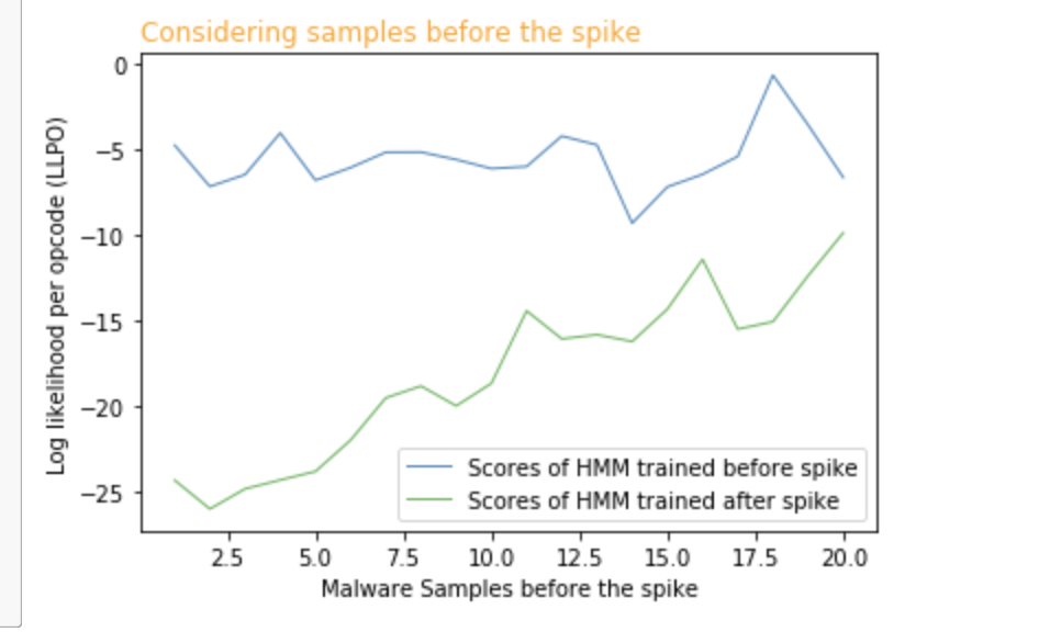
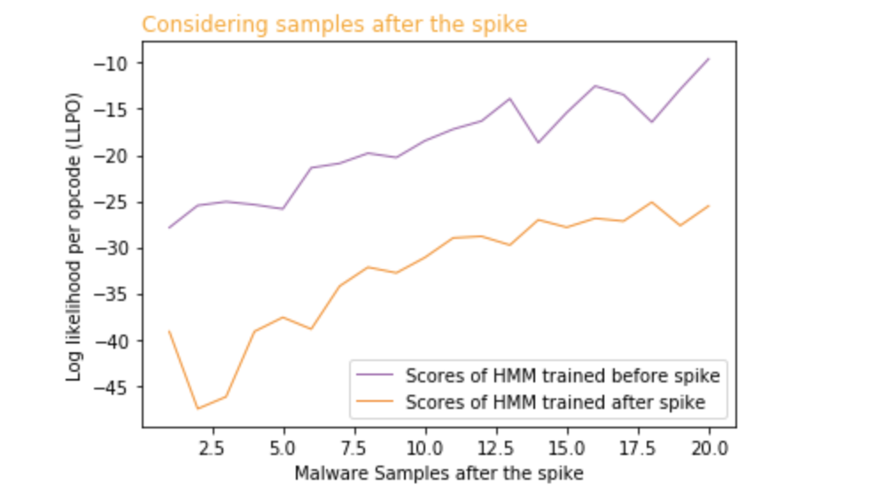
(a) Malware samples before spike	(b) Malware samples after spike

Figure 3: Hidden Markov model trained before and after the spike

In both Figure 3 (a) and (b) we see that the scores are distinct for the two models on each sample tested. These results demonstrates that the model trained before and the model trained after the spike are significantly different which, in turn, indicates that the samples used to train the models differ significantly. This is a clear sign of an evolutionary branch point in the malware family.

4.2 Opcode-SVM Results

In this section, we discuss experiments on 15 malware families, based on opcode sequences and SVMs. That is, opcodes sequences are used directly as features in linear SVM models, with the resulting model weights used to compute $\chi^{2}$ graphs.

Figure 4 gives such a $\chi^{2}$ graph for the Zegost family, which has 506 malware samples from the years 2008 through 2011. We observe multiple spikes in the graph but the secondary HMM test does not yield impressive results for any of these spikes. Hence, we conclude that this particular test does not reveal any strong evolution result for the Zegost family.

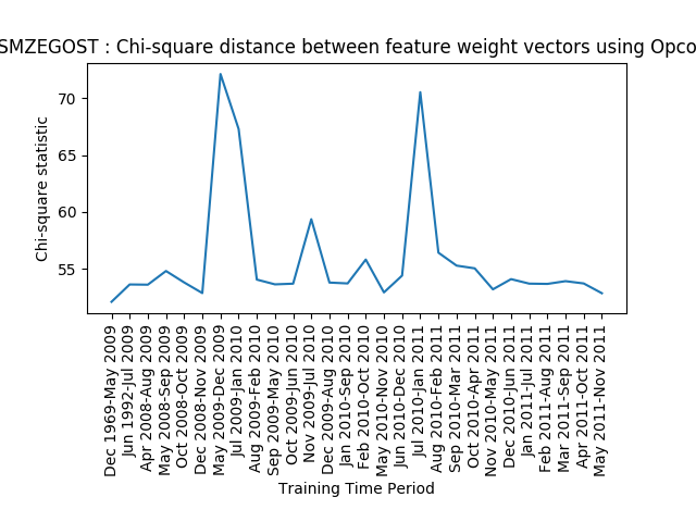
Figure 4: Opcode-SVM $\chi^{2}$ similarity graph for Zegost

We also computed opcode-SVM $\chi^{2}$ graphs for the remaining 14 malware families, nine of which appear in Figure 5. For Adload and BHO, we observe that the graphs do not show any significant spikes except at the last time period. We are not able to perform the secondary HMM test at the extreme endpoint, so we are not able to confirm or deny these as evolution points.

From Figure 5, we observe considerable fluctuation in the graphs for Bifrose, CeeInject, Hupigon, and Rbot, but none of these fluctuations stand out as clear points of possible evolutionary change in the families. That is, for these families, it appears that we only observe background noise.

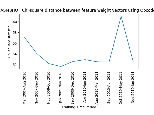
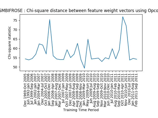
(a) Adload	(b) BHO	(c) Bifrose
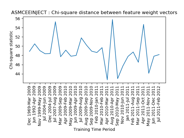
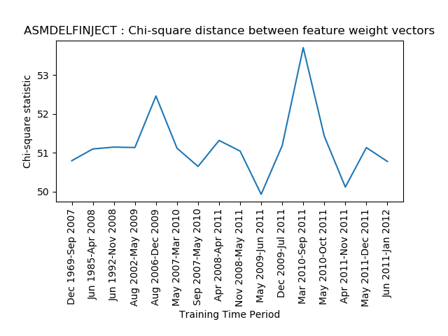
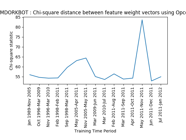
(d) CeeInject	(e) DelfInject	(f) Dorkbot
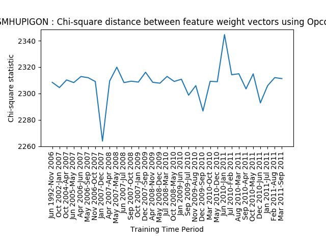
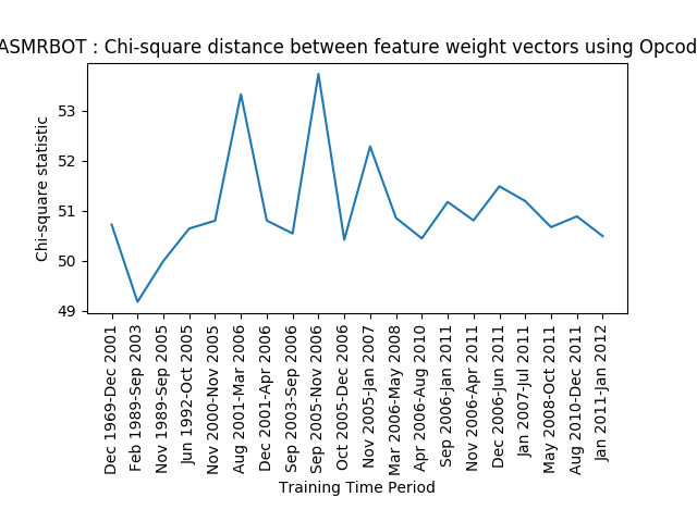
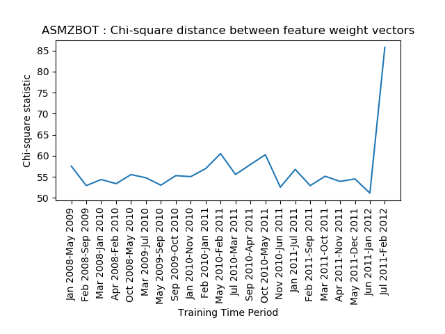
(g) Hupigon	(h) Rbot	(i) Zbot

Figure 5: Opcode-SVM $\chi^{2}$ graphs for selected families

4.3 Opcode $n$-gram-SVM Results

Next, we consider analogous experiments to those of the previous section, but based on opcode $n$-grams. This can be viewed as a first attempt at feature engineering. As with the previous experiments, we train linear SVMs on these features and construct $\chi^{2}$ graphs. We consider overlapping $n$-grams, and we experimented with $n=2,3,5,10$ on each of the 15 families.

Examples of the results of these $n$-gram experiments are given in Figure 6, which shows $2$-gram and $5$-gram $\chi^{2}$ graphs for the Zegost family. For both of these cases, we see only noisy results, with no clear evolutionary points. These results are typical of our $n$-gram experiments and we conclude that opcode $n$-grams are not useful for our purposes.

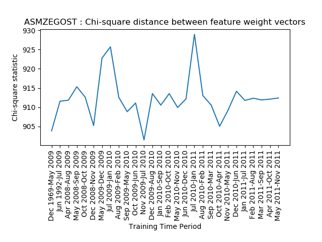
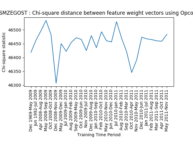
(a) Zegost 2-gram		(b) Zegost 5-gram

Figure 6: Opcode-$n$-gram-SVM $\chi^{2}$ graphs for Zegost

Next, we consider Word2Vec and HMM2Vec word embeddings These feature engineering techniques prove to be more effective for detecting evolutionary changes, with HMM2Vec giving us our strongest results.

4.4 Opcode-Word2Vec-SVM Results

Here, we generate Word2Vec models based on opcode sequences. We then train linear SVMs over each time window, based on these Word2Vec embeddings, and we compute $\chi^{2}$ graphs of the SVM weights. As above, spikes in this graph indicate points in time where evolution might have occurred.

Figures 7 (a) and (b) gives the $\chi^{2}$ graphs for the Zegost family with Word2Vec embeddings of length 2 and 3, respectively. From Figure 7, we observe that feature weights in certain time windows diverge significantly from their average values. Specifically, these time periods are November 2010 and May 2011, and these are the points in time where significant evolution in the family may have taken place. We also note the similarity between the results for embedding vector lengths 2 and 3. This can be viewed as a sign of the stability of the underlying approach, and serves to provide additional confidence in the putative evolution points.

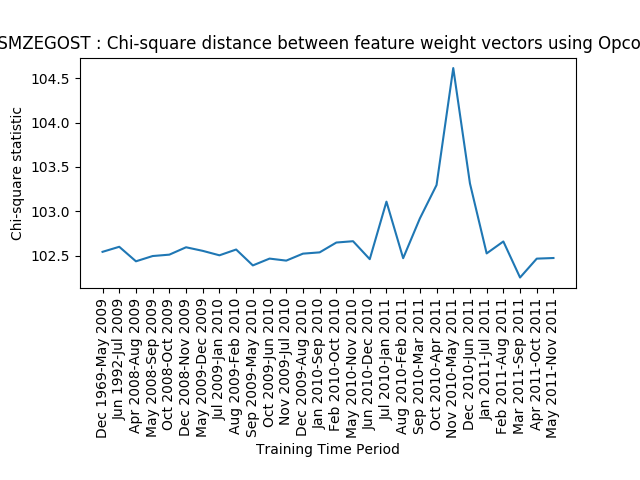
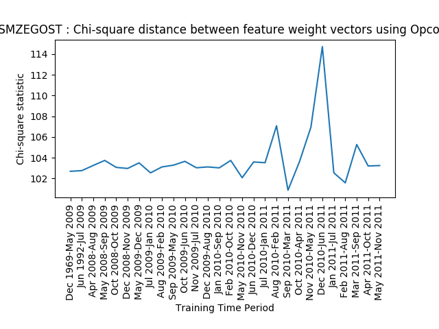
(a) Zegost vector length 2		(b) Zegost vector length 3

Figure 7: Opcode-Word2Vec-SVM $\chi^{2}$ graphs for Zegost

Applying our secondary HMM verification technique to the spike in Figure 7, we obtain the results in Figure 8, which confirm that the malware family has evolved at this point. Since vector lengths of 2 and 3 give us consistent results for Zegost, for our remaining Word2Vec experiments, we use embedding vectors of length 2 in all cases.

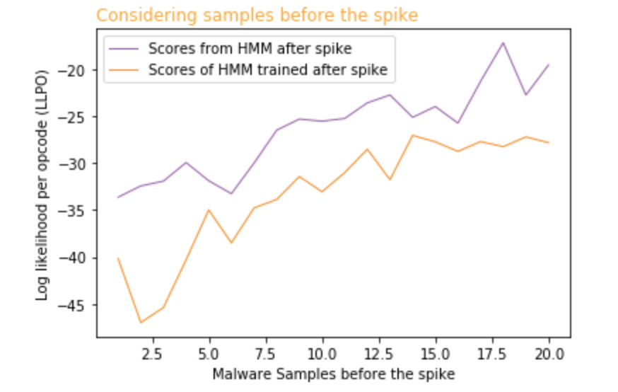
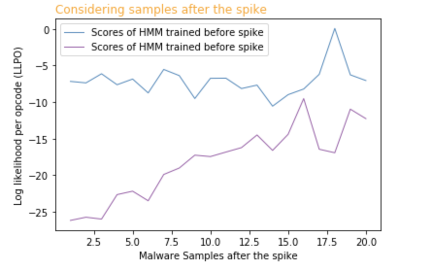
(a) Before spike		(b) After spike

Figure 8: Zegost HMM secondary test for opcode-Word2Vec-SVM

Figure 9 shows our Word2Vec based $\chi^{2}$ graphs for eight additional malware families. Four of these families—BHO, Bifrose, Adload, and Vobfus—perform well with this approach, in the sense that we detect clear spikes in their graphs.

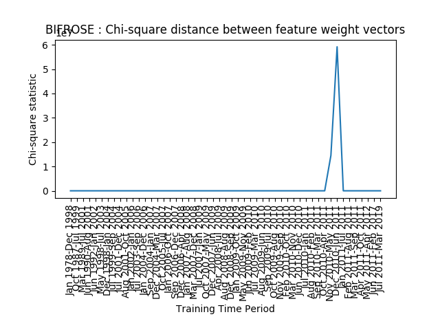
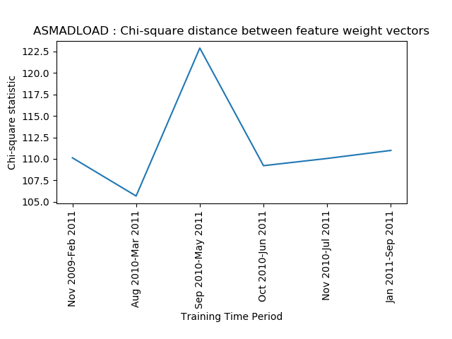
(a) BHO vector size 2	(b) Bifrose vector size 2	(c) Adload vector size 2
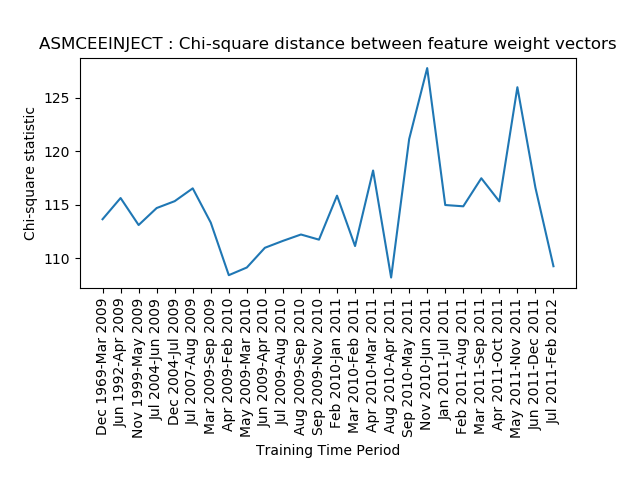
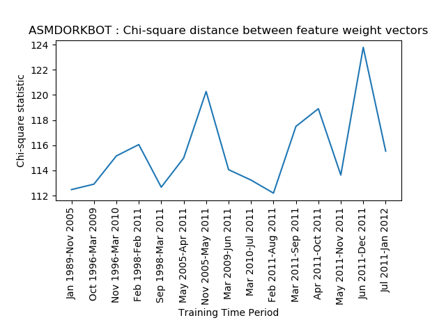
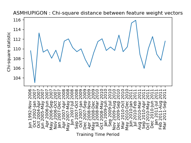
(d) CeeInject vector size 2	(e) Dorkbot vector size 2	(f) Hupigon vector size 2
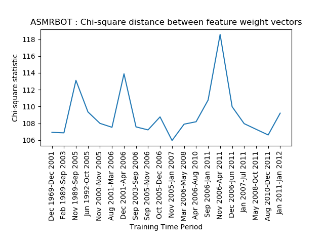
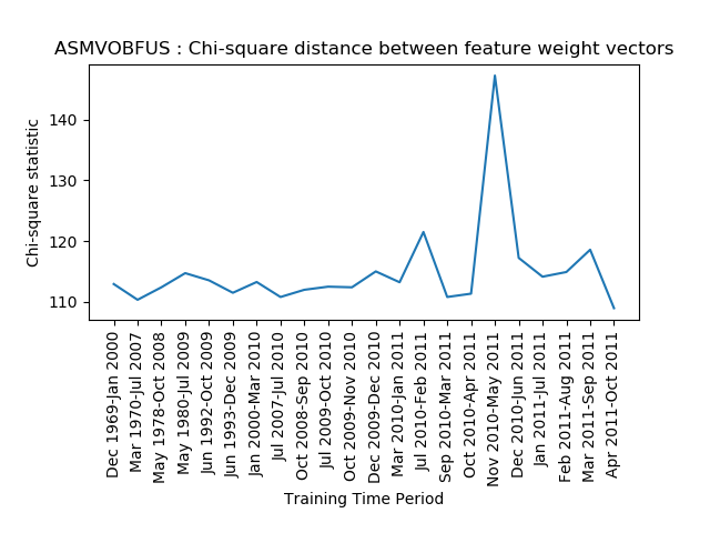
(g) Rbot vector size 2 (h) Vobfus vector size 3

Figure 9: Opcode-Word2Vec-SVM $\chi^{2}$ graphs for selected families

For the remaining four families in Figure 9, namely, CeeInject, Dorkbot, Hupigon, and Rbot, we do not detect any significant spikes in their $\chi^{2}$ graphs. Additional secondary HMM tests showing evolution appear in Figure 10, while Figure 11 gives an example of a secondary test that shows no evolution. It is evident that the results of these opcode-Word2Vec-SVM experiments are a major improvement over the experiments considered above.

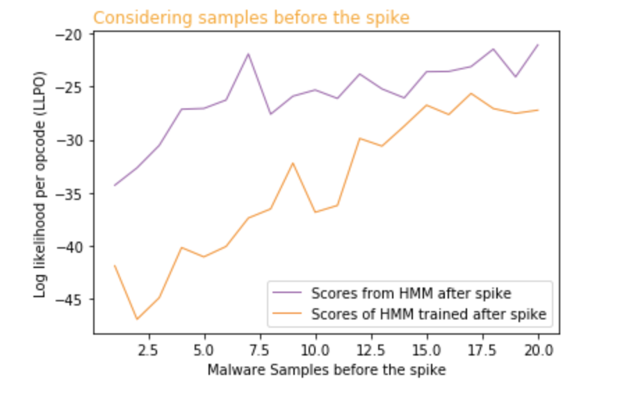
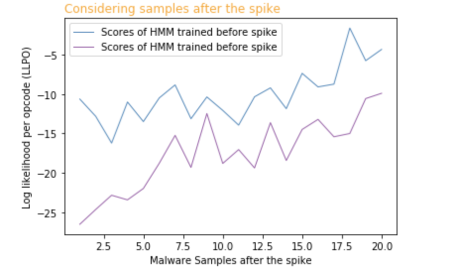
(a) BHO before spike		(b) BHO after spike
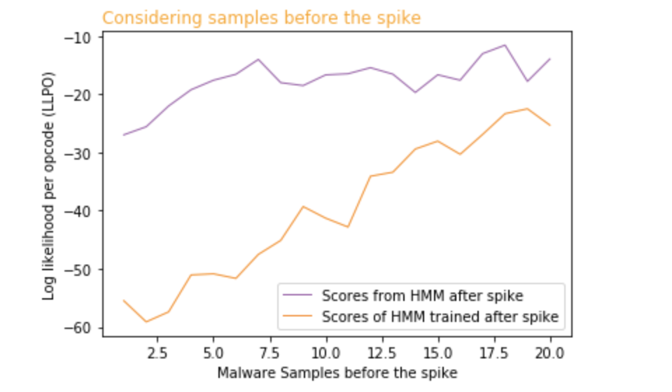
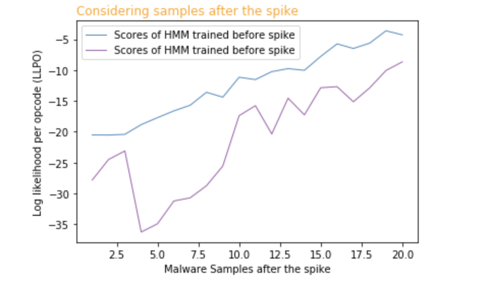
(c) Vobfus before spike		(d) Vobfus after spike

Figure 10: HMM secondary tests for opcode-Word2Vec-SVM showing evolution

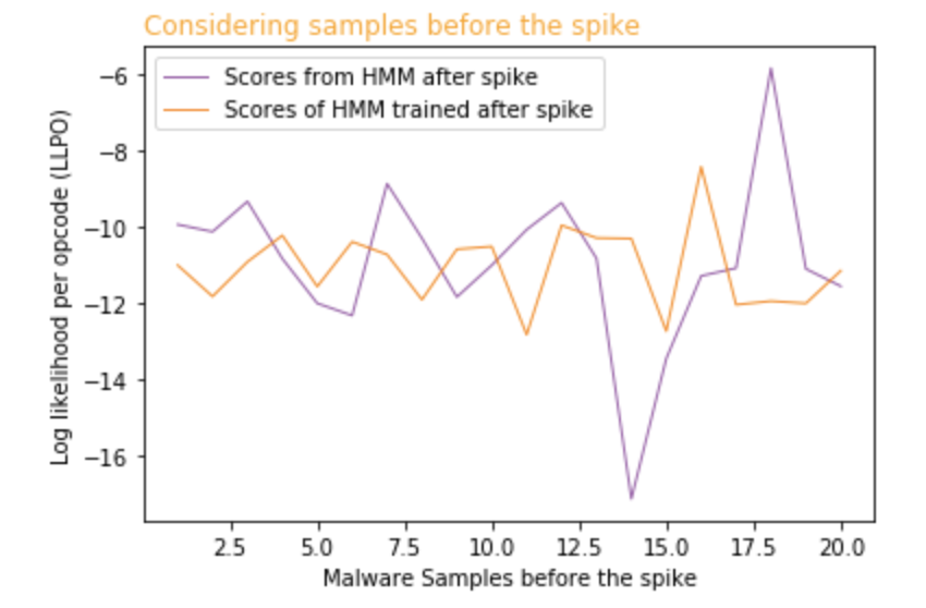
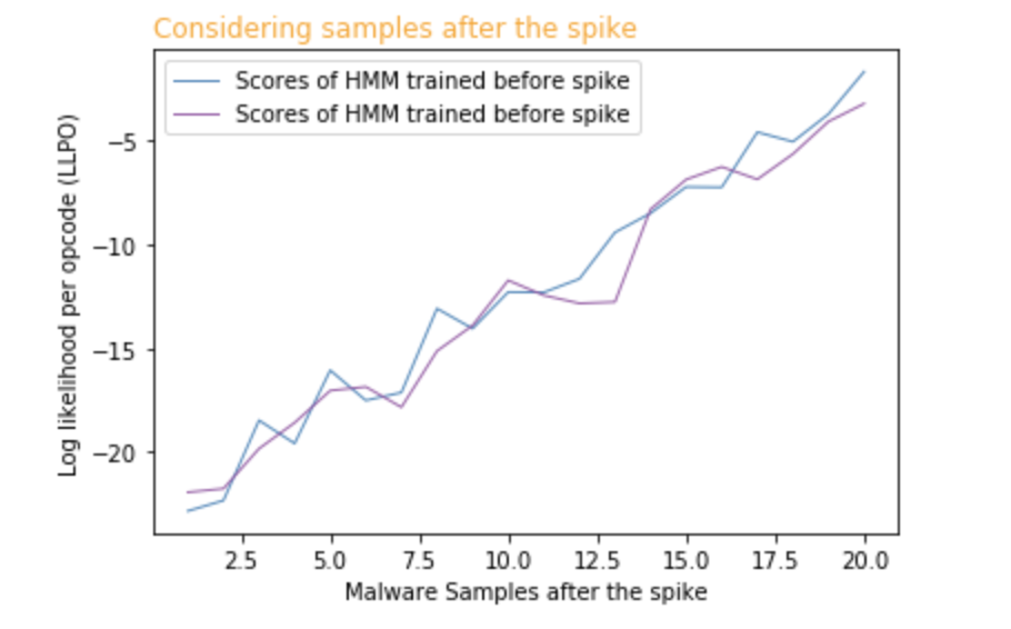
(a) CeeInject before spike		(b) CeeInject after spike

Figure 11: HMM secondary tests for opcode-Word2Vec-SVM showing no evolution

Of course, it is possible that there is no evolution to be detected, in some of these families. But, over the extended time periods under consideration, we believe it likely that evolution has occurred, which suggests that the Word2Vec features are simply not sufficiently sensitive to detect changes in all cases. In the next section, we consider another word embedding technique.

4.5 Opcode-HMM2Vec-SVM Results

The experiments in this section are essentially the same as those in the previous section, except that we use HMM2Vec embeddings in place of Word2Vec embeddings. As discussed above, HMM2Vec embeddings use obtained from the $B$ matrix of a trained HMM.

Figures 12 (a) and (b) give HMM2Vec based $\chi^{2}$ graphs for Zegost, using one random start and 10 random restarts, respectively. Note that these results are based on HMMs with $N=2$ hidden states, which gives us embedding vectors of length 2. Since our HMM training algorithm is a hill climb technique, multiple random restarts often enable us to find a stronger model. For the Zegost results in Figure 12, random restarts appear to offer little, if any, advantage. Consequently, for the remaining experiments in this section, we train a single HMM model, and we do not perform any random restarts.

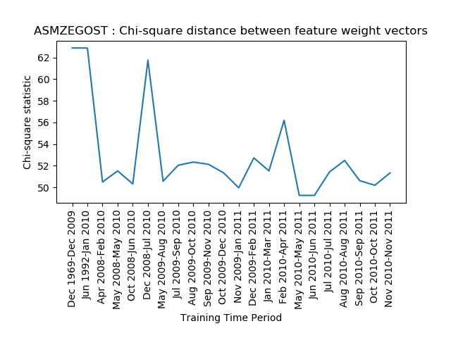
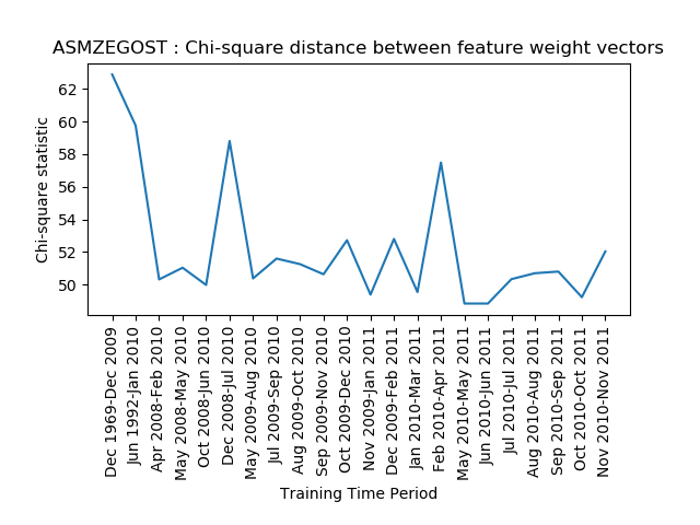
(a) Zegost without restarts		(b) Zegost with 10 restarts

Figure 12: Opcode-HMM2Vec-SVM $\chi^{2}$ graphs for Zegost

We experimented with $N=2$ and $N=3$ hidden states (giving us embedding vectors of length 2 and 3, respectively), but we did not find any improvement using $N=3$. Hence, we use HMM2Vec embedding vectors of length 2 in all experiments below.

Figure 13 shows the $\chi^{2}$ graphs for 8 additional families based on HMM2Vec embedding vectors. Overall, this HMM2Vec-SVM approach seems to provide better results than the Word2Vec-SVM technique in the previous section, as we can detect more malware evolution using the HMM2Vec feature engineering.

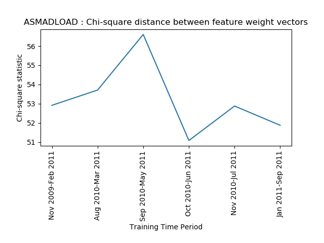
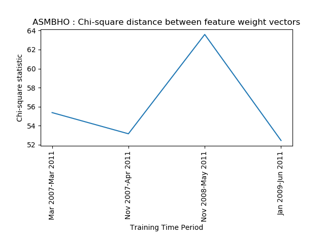
(a) Adload	(b) Zbot	(c) BHO
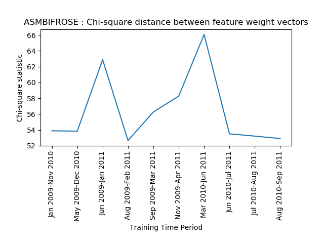
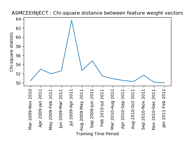
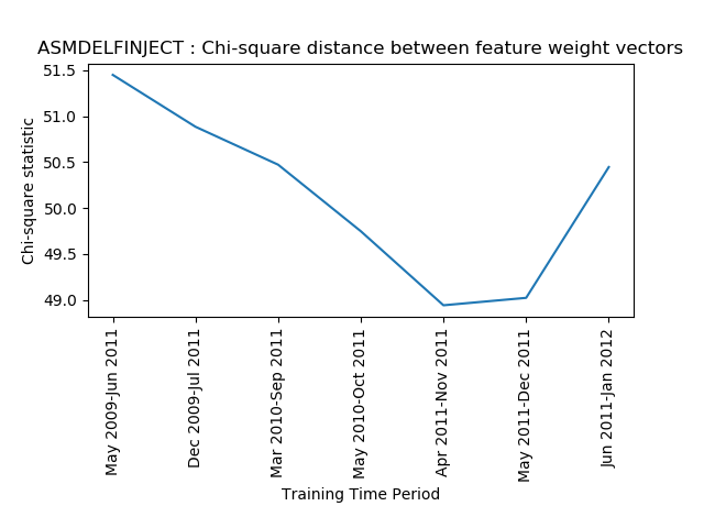
(d) Bifrose	(e) CeeInject	(f) DelfInject
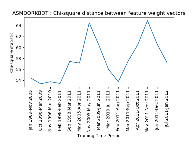
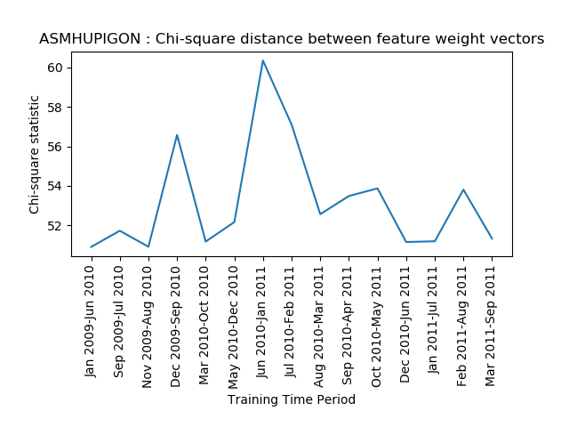
(g) Dorkbot (h) Hupigon

Figure 13: Opcode-HMM2Vec-SVM $\chi^{2}$ for selected families

Based on the graphs in Figure 13, we make the following observations.

Adload

— An evolutionary event takes place in the time window Sep 2010–May 2011.

Zbot

— No significant spike is observed in the $\chi^{2}$ graph.

BHO

— Significant evolution takes place in the time window Nov 2008–May 2011

Bifrose

— Malware evolution takes place in the time window March 2010–June 2011. The other spike in the period June 2009–Jan 2011 is a part of noise in the data. This was confirmed by training HMMs on both sides.

CeeInject

— Evolution occurs in the time window June 2009–April 2011.

DelfInject

— No significant spike is observed in the $\chi^{2}$ graph.

Dorkbot

— No significant spike is observed in the $\chi^{2}$ graph.

Hupigon

— A significant spike in the time period June 2010–Jan2011 is observed in the graph.

From Figure 13 we conclude that we can observe significant spikes in almost all families using HMM2Vec-SVM analysis. For the families Adload, BHO, Bifrose, CeeInject, and Hupigon we observe significant spikes in the $\chi^{2}$ distribution graph. HMM secondary test confirming evolution for some of these cases appear in Figure 14. In Figure 15, we give results of HMM secondary tests that do not reveal evolution.

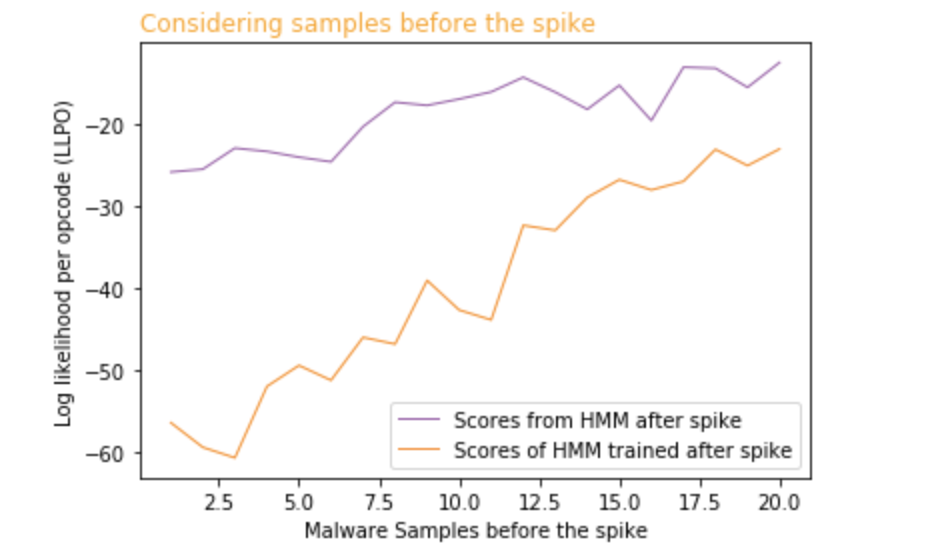
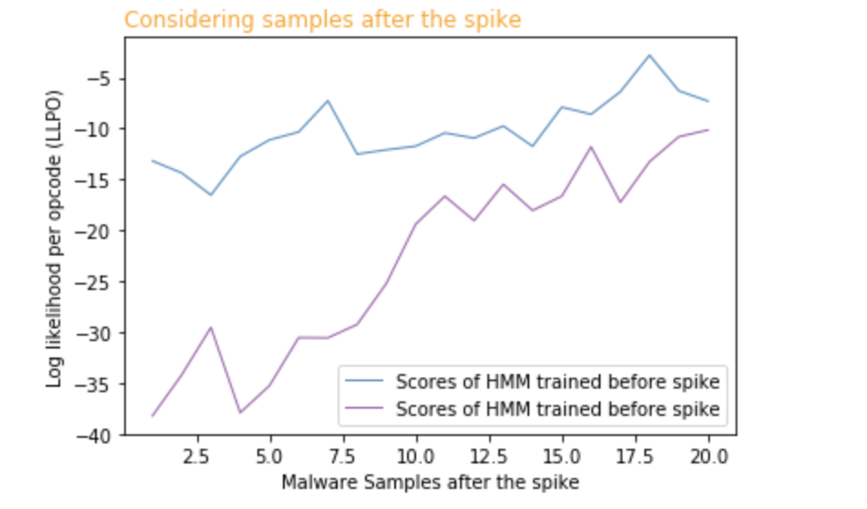
(a) BHO before spike		(b) BHO after spike
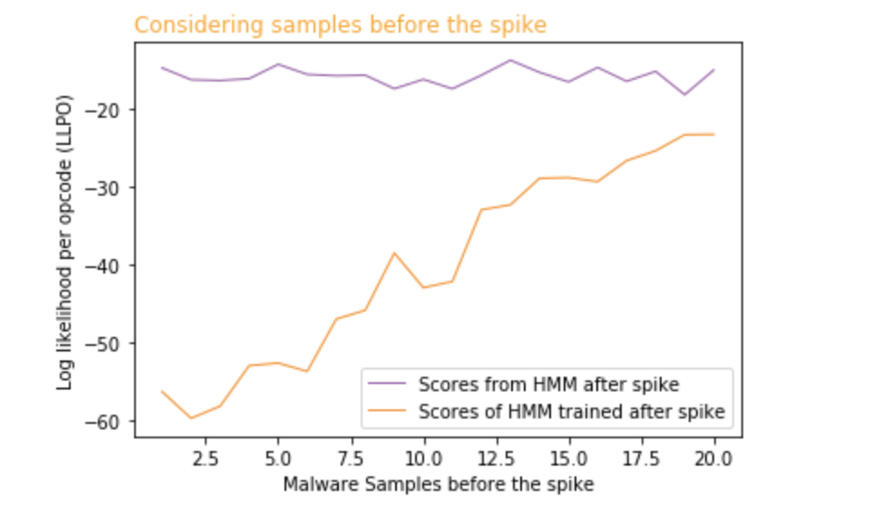
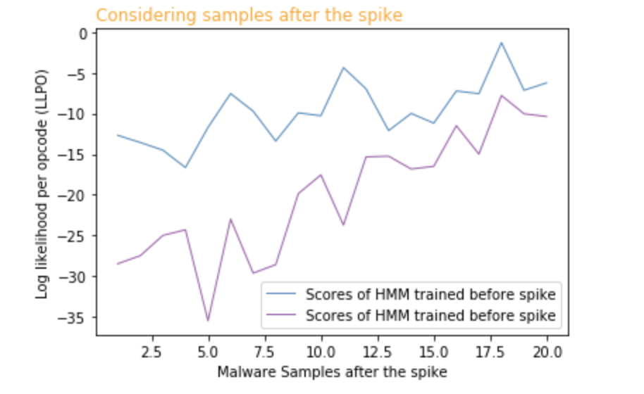
(c) Bifrose before spike		(d) Bifrose after spike
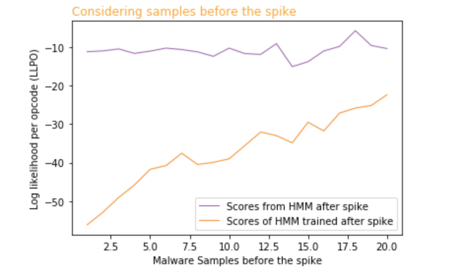
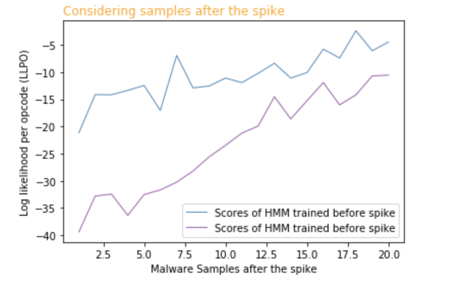
(e) CeeInject before spike		(f) CeeInject after spike
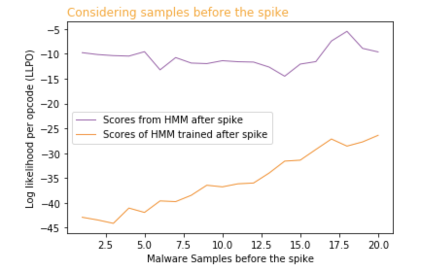
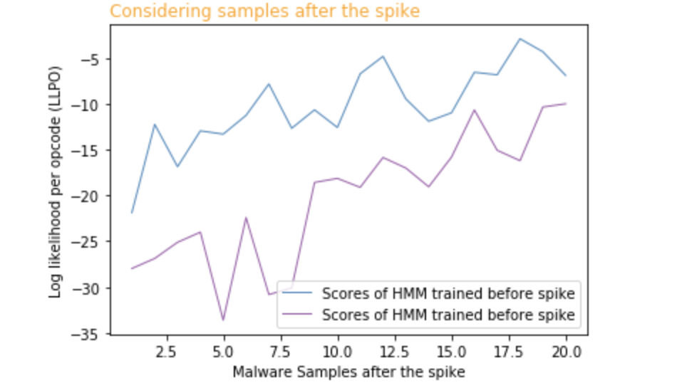
(g) Hupigon before spike		(h) Hupigon after spike

Figure 14: HMM secondary tests for opcode-HMM2Vec-SVM showing evolution

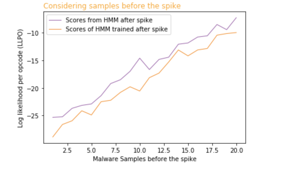
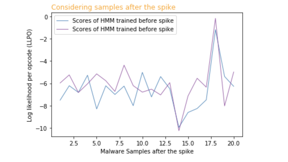
(a) DelfInject before dip		(b) DelfInject after dip
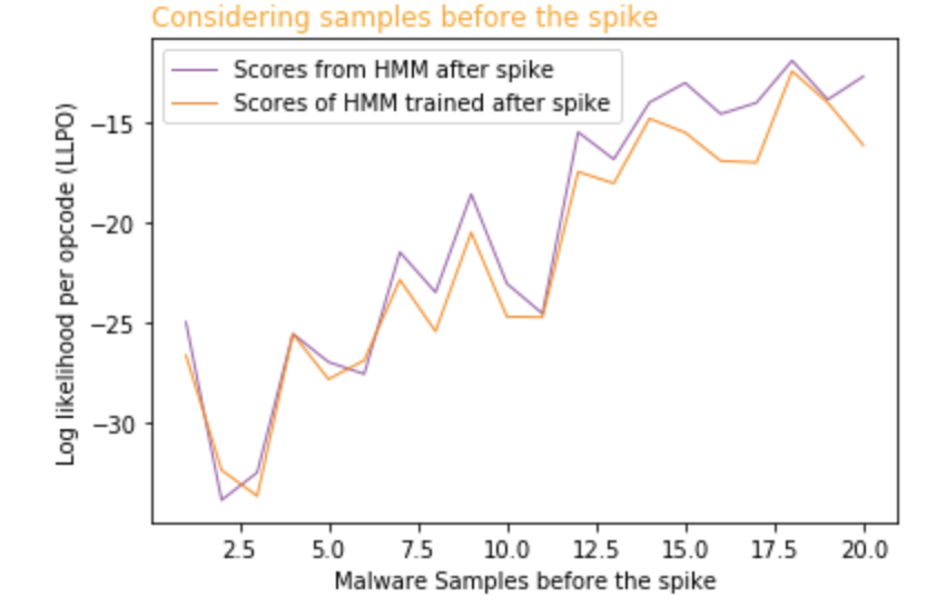
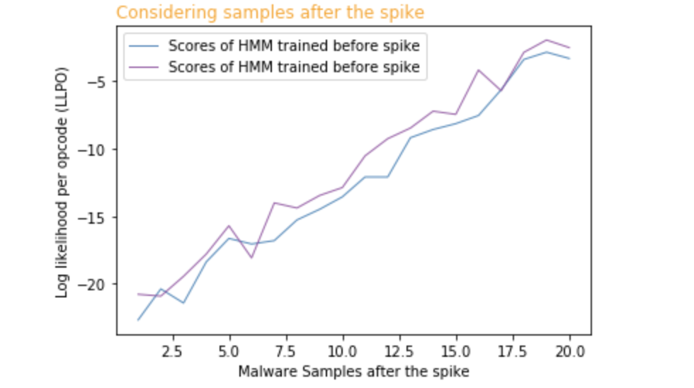
(c) Dorkbot before first spike		(d) Dorkbot after first spike

Figure 15: HMM secondary tests for opcode-HMM2Vec-SVM showing no evolution

Comparing the families in which we could detect evolutionary changes using Word2Vec with those detected using HMM2Vec, we observe that the evolutionary points obtained using Word2Vec are also found using HMM2Vec. Yet, the HMM2Vec technique provides additional evolutionary points, indicating that it is more sensitive to change than Word2Vec embeddings. Overall, HMM2Vec performed better than any of the other approaches that we considered in this paper.

5 Conclusion and Future Work

Previous research has shown that analysis based on PE file features and linear SVM models can be useful in detecting malware evolution [29]. In this paper, we expanded on—and improved upon—this previous work in several ways. First, we considered opcode features, rather than PE file features. Our intuition was that opcode based features would be more sensitive to the types of changes that we would like to detect, and our results support this intuition. Second, we experimented with various feature engineering techniques, and we found that vector embeddings increase the sensitivity of the SVM analysis. Thirdly, we showed that a secondary test using HMM techniques can be used to verify that suspected evolutionary points in the timeline.

We experimented with a variety of techniques, and our best results were obtained using an approach that we refer to as opcode-HMM2Vec-SVM. In this technique, we use mnemonic opcodes as raw features, then generate HMM2Vec encodings of the opcodes, which serve as features for linear SVMs, with the SVMs trained over sliding windows of time. The resulting SVM weights are compared using a $\chi^{2}$ statistic, and we graph this statistic over the available timeline. Spikes in the $\chi^{2}$ graph serve as indicators of likely evolutionary change. We were then able to further confirm evolutionary changes using a secondary test based on training HMMs on either side of a spike. This overall approach was more sensitive than previous work, in the sense that we were able to detect additional changes in the codebase of various families, and it was more precise, since we have a secondary test available to confirm (or deny) putative evolutionary changes.

In the realm of future work, additional machine learning techniques and additional features and engineering strategies could be considered. For example, neural network techniques could be used in place of SVMs, with multiclass output probabilities playing the role of the linear SVM weights. Another option would be to elevate our HMM-based secondary test to the role of the primary test. This might enable a more fine-grained analysis of the timeline, as relatively little data is needed for HMM training. With respect to feature engineering, dimensionality reduction techniques would be a natural topic to consider. The use of dynamic features might add value as well, although the additional complexity involved with collecting such features might be a concern.

References

- [1] John Aycock. Computer Viruses and Malware. Springer, 2010.
- [2] Jin Bai, Shi Mu, and Guo Zou. The application of machine learning to study malware evolution. Applied Mechanics and Materials, 530-531(Advances in Measurements and Information Technologies):875–878, 2014.
- [3] Marius Barat, Dumitru-Bogdan Prelipcean, and Dragoş Gavriluţ. A study on common malware families evolution in 2012. Journal of Computer Virology and Hacking Techniques, 9(4):171–178, 2013.
- [4] Zhongqiang Chen, Mema Roussopoulos, Zhanyan Liang, Yuan Zhang, Zhongrong Chen, and Alex Delis. Malware characteristics and threats on the internet ecosystem. The Journal of Systems & Software, 85(7):1650–1672, 2012.
- [5] Anusha Damodaran, Fabio Troia, Corrado Visaggio, Thomas Austin, and Mark Stamp. A comparison of static, dynamic, and hybrid analysis for malware detection. Journal of Computer Virology and Hacking Techniques, 13(1):1–12, 2017.
- [6] Julian Gilyadev. Word2vec explained. https://israelg99.github.io/2017-03-23-Word2Vec-Explained/, 2017.
- [7] A Gupta, P Kuppili, A Akella, and P Barford. An empirical study of malware evolution. In 2009 First International Communication Systems and Networks and Workshops, pages 1–10. IEEE, 2009.
- [8] Samuel Kim. PE header analysis for malware detection. Master’s thesis, San Jose State University, Department of Computer Science, 2018.
- [9] Francesco Mercaldo, Andrea Di Sorbo, Corrado Aaron Visaggio, Aniello Cimitile, and Fabio Martinelli. An exploratory study on the evolution of android malware quality. Journal of Software: Evolution and Process, 30(11):n/a–n/a, 2018.
- [10] Microsoft. Win32 rbot detected with windows defender antivirus. https://www.microsoft.com/en-us/wdsi/threats/malware-encyclopedia-description?Name=Win32%2FRbot, 2005.
- [11] Microsoft. Adware: Win32 hotbar detected with windows defender antivirus. https://www.microsoft.com/en-us/wdsi/threats/malware-encyclopedia-description?Name=Adware%3AWin32%2FHotbar, 2006.
- [12] Microsoft. Backdoor: Win32 hupigon detected with windows defender antivirus. https://www.microsoft.com/en-us/wdsi/threats/malware-encyclopedia-description?Name=Backdoor%3AWin32%2FHupigon, 2006.
- [13] Microsoft. Virtool: Win32 ceeinject detected with windows defender antivirus. https://www.microsoft.com/en-us/wdsi/threats/malware-encyclopedia-description?Name=VirTool%3AWin32%2FCeeInject, 2007.
- [14] Microsoft. Virtool: Win32 delfinject detected with windows defender antivirus. https://www.microsoft.com/en-us/wdsi/threats/malware-encyclopedia-description?Name=VirTool:Win32/DelfInject&ThreatID=-2147369465, 2007.
- [15] Microsoft. Virtool: Win32 vbinject detected with windows defender antivirus. https://www.microsoft.com/en-us/wdsi/threats/malware-encyclopedia-description?Name=VirTool:Win32/VBInject&ThreatID=-2147367171, 2010.
- [16] Microsoft. Win32 vobfus detected with windows defender antivirus. https://www.microsoft.com/en-us/wdsi/threats/malware-encyclopedia-description?name=win32%2Fvobfus, 2010.
- [17] Microsoft. Win32 winwebsec detected with windows defender antivirus. https://www.microsoft.com/security/portal/threat/encyclopedia/entry.aspx?Name=Win32%2fWinwebsec, 2010.
- [18] Microsoft. Win32 obfuscator detected with windows defender antivirus. https://www.microsoft.com/en-us/wdsi/threats/malware-encyclopedia-description?Name=Win32%2FObfuscator, 2011.
- [19] Microsoft. Win32 zbot detected with windows defender antivirus. http://www.symantec.com/securityresponse/writeup.jsp?docid=2010-011016-3514-99, 2011.
- [20] Microsoft. Win32 zegost detected with windows defender antivirus. https://www.symantec.com/security-center/writeup/2011-060215-2826-99, 2011.
- [21] Microsoft. Worm: Win32 dorkbot detected with windows defender antivirus. https://www.microsoft.com/en-us/wdsi/threats/malware-encyclopedia-description?Name=Worm%3AWin32/Dorkbot, 2011.
- [22] Microsoft. Win32 bifrose detected with windows defender antivirus. https://www.trendmicro.com/vinfo/us/threat-encyclopedia/malware/bifrose, 2012.
- [23] Antonio Nappa, M. Rafique, and Juan Caballero. The malicia dataset: identification and analysis of drive-by download operations. International Journal of Information Security, 14(1):15–33, 2015.
- [24] J. Ouellette, A. Pfeffer, and A. Lakhotia. Countering malware evolution using cloud-based learning. Proceedings of the 8th international conference on malicious and unwanted software, page 85–94, 2013.
- [25] Igor Popov. Malware detection using machine learning based on word2vec embeddings of machine code instructions. In 2017 Siberian Symposium on Data Science and Engineering (SSDSE), pages 1–4. IEEE, 2017.
- [26] Saeid Rezaei, Fereidoon Rezaei, Ali Afraz, and Mohammad Reza Shamani. Malware detection using opcodes statistical features. In 2016 8th International Symposium on Telecommunications (IST), pages 151–155. IEEE, 2016.
- [27] Mark Stamp. Introduction to machine learning with applications in information security. CRC Press, Taylor & Francis Group, Boca Raton, FL, 2018.
- [28] Mark Stamp. Alphabet soup of deep learning topics. https://www.cs.sjsu.edu/~stamp/RUA/alpha.pdf, 2019.
- [29] Mayuri Wadkar, Fabio Di Troia, and Mark Stamp. Detecting malware evolution using support vector machines. Expert Systems with Applications, 143, 2020.