GUP corrected entropy of the Schwarzschild black hole in holographic massive gravity

Abstract

We obtain the statistical entropy of a scalar field on the Schwarzschild black hole in holographic massive gravity by considering corrections on the density of quantum states to all orders in the Planck length from a generalized uncertainty principle (GUP). As a result, we find not only the generalized Bekenstein-Hawking entropy depending on holographically massive gravitons without any artificial cutoff, but also new additional correction terms, which are proportional to surface gravity. Moreover, we also observe that all order GUP corrected entropy is improved to have smaller GUP parameter $\lambda$ than the previous results.

I introduction

Einstein’s theory of general relativity (GR) is a theory of a massless spin-2 graviton, which has been successfully tested to date as the description of the force of gravity. However, quantum gravity phenomenology AmelinoCamelia:2008qg that focuses on modifications of the existing theory at extreme limits has pushed forward to search for alternatives to GR. One of them is to introduce a massive graviton to GR. In 1930s, by extending GR with a quadratic mass term, Fierz and Pauli developed a massive spin-2 theory Fierz:1939ix . It was later known to suffer from the Boulware-Deser ghost problem Boulware:1973my and the van Dam, Veltman and Zakharov (vDVZ) discontinuity vanDam:1970vg ; Zakharov:1970cc in the massless graviton limit. The vDVZ discontinuity was cured by the Vainshtein mechanism Vainshtein:1972sx due to certain low scale strongly coupled interactions. Moreover, de Rham, Gabadadze and Trolley (dRGT) deRham:2010ik ; deRham:2010kj successfully obtained a ghost free massive gravity, which has nonlinearly interacting mass terms constructed from the metric coupled with a symmetric reference metric tensor. This was confirmed by a Hamiltonian analysis of the untruncated theory Hassan:2011hr ; Hassan:2011tf and other works Kluson:2011qe ; Kluson:2011rt ; Kluson:2012gz ; Comelli:2012vz ; Golovnev:2011aa ; Deffayet:2012nr . Furthermore, Vegh Vegh:2013sk introduced a nonlinear massive gravity with a special singular reference metric which keeps the diffeomorphism symmetry for coordinates ($t,r$) intact but breaks it in angular directions so that gravitons acquire the mass because of a broken momentum conservation Davison:2013jba ; Blake:2013bqa ; Blake:2013owa . Since then, this Vegh’s type of massive gravity, called holographic massive gravity, has been extensively exploited to investigate many black hole models Cai:2014znn ; Adams:2014vza ; Hendi:2015pda ; Hu:2016hpm ; Zou:2016sab ; Hendi:2017fxp ; Tannukij:2017jtn ; Hendi:2017bys ; Hendi:2018xuy ; Chabab:2019mlu ; Hong:2018spz . Very recently, we have investigated the tidal effects in the Schwarzschild black hole in holographic massive gravity (SBHHMG), showing that massive gravitons effectively affect the angular component of the tidal force, while the radial component remains the same as in massless gravity Hong:2019zsi .

On the other hand, quantum gravity phenomenology predicts the possible existence of a minimal length on the smallest scale [33]. This implies the modification of the Heisenberg uncertainty principle (HUP) in quantum mechanics to a generalized uncertainty principle (GUP) Kempf:1994su ; Garay:1994en ; Scardigli:1999jh ; KalyanaRama:2001xd ; Chang:2001bm ; Hossenfelder:2012jw , which paves the way for deeper understanding on black hole thermodynamics Adler:2001vs ; Scardigli:2003kr ; Setare:2004sr ; Medved:2004yu ; Ling:2005bq ; Myung:2006qr ; Kim:2016qtp ; Feng:2020lai including the final stage of the Hawking radiation. As is well known, studies on black holes in terms of thermodynamics started with the discovery of the Bekenstein-Hawking entropy Bekenstein:1972tm ; Bekenstein:1973ur ; Bekenstein:1974ax ; Hawking:1974rv ; Hawking:1974sw proportional to the surface area of a black hole at the event horizon. In order to provide a microphysical explanation to the Bekenstein-Hawking entropy, ’t Hooft developed the statistical method of finding the black hole’s entropy by introducing a scalar field propagating just outside the event horizon tHooft:1984kcu . After the pioneering work of ’t Hooft, in the last several decades, a lot of authors have studied statistical properties of various types of black holes Mann:1990fk ; Ghosh:1994wb ; Demers:1995dq ; Cai:1996js ; Kim:1996bp ; Kim:1996eg ; Ho:1997fg ; Mukohyama:1998rf ; Jing:1999bw ; Li:2000rk ; Winstanley:2000in ; Kim:2001kpa ; Medved:2001zw ; Gao:2002ed ; Sun:2004ct ; Kenmoku:2005zh ; Sarkar:2007uz ; Singleton:2010gz ; Eune:2012mv ; Lenz:2014aea ; Eune:2014tea ; Kamali:2016agu ; Kamali:2018 ; Vagenas:2019wzd ; Cuadros-Melgar:2020shz . One of main characteristics in his so-called brick wall method is to introduce an cutoff which removes ultraviolet divergences due to the infinite blue shift at the event horizon. Later, it was shown that the cutoff can be effectively replaced by a minimal length to the order of the Planck length which is derived from a GUP Li:2002xb . Making use of these ideas, the authors in Refs. Zhao:2003eu ; Liu:2004xh ; Kim:2006rx ; Yoon:2007aj have calculated the statistical entropy of black holes to leading order in the Planck length. The ultraviolet divergences of the just vicinity near the horizon in the usual brick wall method is drastically solved by the newly modified equation of the density states motivated by GUPs Kempf:1994su ; Garay:1994en ; Scardigli:1999jh ; KalyanaRama:2001xd ; Chang:2001bm ; Hossenfelder:2012jw . Since the GUP up to leading order correction in the Planck length is not enough because the wave vector $k$ does not satisfy the asymptotic property in the modified dispersion relation Hossenfelder:2006cw ; Hossenfelder:2005ed , Nouicer has further developed the GUP effect to all orders in the Planck length Nouicer:2007jg ; Nouicer:2007cw After his work, according to this approach, we have obtained the desired Bekenstein-Hawking entropy to all orders in the Planck length units without any artificial cutoff and little mass approximation for the case of the Schwarzschild black hole Kim:2007if . However, all of these works have been concentrated on black holes in GR, and it has been rarely studied in alternatives to GR such as massive gravity, as far as we know. Therefore, it would be interesting to extend them to massive gravity.

In this paper, we calculate statistical entropy of a scalar field on the Schwarzschild black hole in holographic massive gravity by imposing GUP effect additionally to all orders in the Planck length. In Sec. II, we briefly recapitulate the formalism for all order corrections of GUP and its relation to existence of minimal length. In Sec. III, we find the solution of the SBHHMG for self-consistency and discuss Hawking temperatures according to mass parameters. In Sec. IV, we consider a scalar field propagating on the SBHHMG , and calculate the generalized entropy to all orders in the Planck length by counting modified density states in the presence of massive gravitons. Finally, summary and discussion are drawn in Sec. V.

II The formalism of all order corrections of GUP and minimal length

Quantum gravity phenomenology has been tackled with effective models which incorporate a minimal length as a natural ultraviolet cutoff Hossenfelder:2006cw ; Hossenfelder:2005ed . Such a minimal length leads to deformed Heisenberg algebras Kempf:1994su ; Garay:1994en ; Scardigli:1999jh ; KalyanaRama:2001xd ; Adler:2001vs which show a GUP. For a particle with the momentum $p$ and the wave vector $k$ having a nonlinear relation $p=f(k)$, the commutator between two operators $\hat{x}$ and $\hat{p}$ can be generalized to

$$[\hat{x},\hat{p}]=i\frac{\partial p}{\partial k}~{}\Leftrightarrow\Delta x\Delta p\geq\frac{1}{2}\left|~{}\left<\frac{\partial p}{\partial k}\right>~{}\right|$$ (2.1)

at the quantum mechanical level Hossenfelder:2006cw ; Hossenfelder:2005ed . Without loss of generality, in the following, let us restrict ourselves to the isotropic case in one space-like dimension.

As a nonlinear dispersion relation, Kempf et al. Kempf:1994su ; Garay:1994en ; Scardigli:1999jh ; KalyanaRama:2001xd ; Adler:2001vs have considered the following relation

$$\frac{\partial p}{\partial k}=1+\lambda p^{2},$$ (2.2)

which came in the context of perturbative string theory. The GUP parameter $\lambda$ is of order of the Planck length $l^{-2}_{p}$. By solving the GUP in Eq. (2.1), one can find that it exhibits the features of UV/IR correspondence such that as $\Delta p$ is large, $\Delta x$ is proportional to $\Delta p$. More importantly, it provides us the existence of the minimal length as $(\Delta x)^{\rm Kempf}_{\rm min}=2\sqrt{\lambda}$ below which spacetime distances cannot be resolved.

On the other hand, the GUP of Kempf et al. was extended to all orders in the Planck length Smailagic:2003yb ; Smailagic:2003rp ; Nouicer:2007hz as

$$\frac{\partial p}{\partial k}=~{}e^{\lambda p^{2}}.$$ (2.3)

For this case, the GUP in Eq. (2.1) for mirror symmetric states as $\langle\hat{p}\rangle=0$ can be solved by the multi-valued Lambert function Corless:1996zz . In order to have a real solution for $\Delta p$, it is required to satisfy the following position uncertainty Kim:2007if ; Smailagic:2003yb ; Smailagic:2003rp ; Nouicer:2007hz

$$\Delta x\geq\sqrt{\frac{e\lambda}{2}}.$$ (2.4)

Therefore, one can readily rewrite the minimal length $(\Delta x)_{\rm min}=\sqrt{e/8}(\Delta x)^{\rm Kempf}_{\rm min}$ for the GUP to the all orders in the Planck length.

Note that this includes the leading order correction in the relation (2.2). However, since this correction only of the GUP does not satisfy the property that the wave vector $k$ asymptotically reaches the cutoff in large energy region as in Ref. Hossenfelder:2006cw ; Hossenfelder:2005ed , we will consider the all order corrections in the Planck length in the followings.

III Hawking temperature of the SBHHMG

The (3+1)-dimensional SBHHMG Vegh:2013sk ; Davison:2013jba ; Blake:2013bqa ; Blake:2013owa ; Cai:2014znn ; Adams:2014vza ; Hendi:2015pda ; Hu:2016hpm ; Zou:2016sab ; Hendi:2017fxp ; Tannukij:2017jtn ; Hendi:2017bys ; Hendi:2018xuy ; Chabab:2019mlu ; Hong:2018spz ; Hong:2019zsi is described by the action

$$S=\frac{1}{16\pi G}\int d^{4}x\sqrt{-g}\left[{\cal R}+{\tilde{m}}^{2}\sum_{a=1}^{4}c_{a}{\cal U}_{a}(g_{\mu\nu},f_{\mu\nu})\right],$$ (3.5)

where ${\cal R}$ is the scalar curvature of the metric $g_{\mu\nu}$, $\tilde{m}$ is a graviton mass, $c_{a}$ are constants, and ${\cal U}_{a}$ are symmetric polynomial potentials of the eigenvalue of the matrix ${\cal K}^{\mu}_{\nu}\equiv\sqrt{g^{\mu\alpha}f_{\alpha\nu}}$ as

$${\cal U}_{1} = [{\cal K}],$$

$${\cal U}_{2} = [{\cal K}]^{2}-[{\cal K}^{2}],$$

$${\cal U}_{3} = [{\cal K}]^{3}-3[{\cal K}][{\cal K}^{2}]+2[{\cal K}^{3}],$$

$${\cal U}_{4} = [{\cal K}]^{4}-6[{\cal K}^{2}][{\cal K}]^{2}+8[{\cal K}^{3}][{\cal K}]+3[{\cal K}^{2}]^{2}-6[{\cal K}^{4}].$$ (3.6)

Here, the square root in ${\cal K}$ means $(\sqrt{A})^{\mu}_{\alpha}(\sqrt{A})^{\alpha}_{\nu}=A^{\mu}_{\nu}$ and square brackets denote the trace $[{\cal K}]={\cal K}^{\mu}_{\mu}$. Indices are raised and lowered with the dynamical metric $g_{\mu\nu}$, while the reference metric $f_{\mu\nu}$ is a non-dynamical, fixed symmetric tensor which is introduced to construct nontrivial interaction terms in holographic massive gravity.

Variation of the action (3.5) with respect to the metric $g_{\mu\nu}$ leads to the equations of motion given by

$${\cal R}_{\mu\nu} - \frac{1}{2}g_{\mu\nu}\left({\cal R}+\tilde{m}^{2}\sum^{4}_{a=1}c_{a}{\cal U}_{a}\right)$$ (3.7)

$$+ \frac{1}{2}\tilde{m}^{2}\sum^{4}_{a=1}\left[ac_{a}{\cal U}_{a-1}{\cal K}_{\mu\nu}-a(a-1)c_{a}{\cal U}_{a-2}{\cal K}^{2}_{\mu\nu}+6(3a-8)c_{a}{\cal U}_{a-3}{\cal K}^{3}_{\mu\nu}-12(a-2)c_{a}{\cal U}_{a-4}{\cal K}^{4}_{\mu\nu}\right]=0.$$

with ${\cal U}_{-a}=0$ and ${\cal U}_{0}=1$.

When one considers the spherically symmetric black hole solution ansatz as

$$ds^{2}=-f(r)dt^{2}+f^{-1}(r)dr^{2}+r^{2}(d\theta^{2}+\sin^{2}\theta d\phi^{2})$$ (3.8)

with the following degenerate reference metric Vegh:2013sk ; Davison:2013jba ; Blake:2013bqa ; Blake:2013owa ; Cai:2014znn ; Adams:2014vza ; Hendi:2015pda ; Hu:2016hpm ; Zou:2016sab ; Hendi:2017fxp ; Tannukij:2017jtn ; Hendi:2017bys ; Hendi:2018xuy ; Chabab:2019mlu ; Hong:2018spz

$$f_{\mu\nu}={\rm diag}(0,0,c^{2}_{0},c^{2}_{0}\sin^{2}\theta),$$ (3.9)

one can find

$${\cal K}^{\theta}_{\theta}={\cal K}^{\phi}_{\phi}=\frac{c_{0}}{r}.$$ (3.10)

Note that the choice of the reference metric in Eq. (3.9) preserves general covariance in ($t,r$) but not in the angular directions. This gives the symmetric potentials as

$${\cal U}_{1}=\frac{2c_{0}}{r},~{}~{}~{}{\cal U}_{2}=\frac{2c^{2}_{0}}{r^{2}},~{}~{}~{}{\cal U}_{3}={\cal U}_{4}=0.$$ (3.11)

It should be pointed out that there are no contributions from $c_{3}$ and $c_{4}$ terms which appear in (4+1) and (5+1)-dimensional spacetimes, respectively Cai:2014znn ; Hendi:2015pda ; Hu:2016hpm ; Zou:2016sab ; Hendi:2017fxp ; Hendi:2018xuy . Then, one can have the solution

$$f(r)=1-\frac{2m}{r}+2Rr+{\cal C}$$ (3.12)

with $R=c_{0}c_{1}\tilde{m}^{2}/4$ and ${\cal C}=c^{2}_{0}c_{2}\tilde{m}^{2}$ Hong:2019zsi , where $m$ is an integration constant related to the mass of the black hole and $c_{0}$ is a positive constant Vegh:2013sk ; Davison:2013jba ; Blake:2013bqa ; Blake:2013owa ; Cai:2014znn ; Adams:2014vza ; Hendi:2015pda ; Hu:2016hpm ; Zou:2016sab ; Hendi:2017fxp ; Tannukij:2017jtn ; Hendi:2017bys ; Hendi:2018xuy ; Chabab:2019mlu ; Hong:2018spz .

Now, by solving $f(r)=0$, one can find the event horizons of the SBHHMG as

$$r_{\pm}=\frac{-(1+{\cal C})\pm\sqrt{16mR+(1+{\cal C})^{2}}}{4R}.$$ (3.13)

The allowed event horizon can be classified according to the relative signs of $R$ and ${\cal C}$ as shown in Table 1. We note that the event horizon $r_{+}$ of the SBHHMG is reduced to $2m$ of the Schwarzschild black hole in massless gravity as $R$ and ${\cal C}\rightarrow 0$. It is also appropriate to comment that in Table 1, $r_{-}$ is discarded since it is either negative or imaginary in each ranges. Only in the special case of ${\cal C}>-1$ and $R=-\frac{(1+{\cal C})^{2}}{16m}$, the physical solution of $r_{-}$ exists and coincides exactly with $r_{+}$. In Table 1, the abbreviation NA denotes that there is no available event horizon in the specified range.

Table 1: Event horizons of the SBHHMG

		${\cal C}>-1$	${\cal C}=-1$	${\cal C}<-1$
$R>0$	(I)	$r_{+}=\frac{1+{\cal C}}{4R}\left(-1+\sqrt{1+\frac{16mR}{(1+{\cal C})^{2}}}~{}\right)$	(II) $r_{+}=\sqrt{\frac{m}{R}}$	(III) $r_{+}=-\frac{1+{\cal C}}{4R}\left(1+\sqrt{1+\frac{16mR}{(1+{\cal C})^{2}}}~{}\right)$
$R=0$	(IV)	$r_{+}=\frac{2m}{1+{\cal C}}$	NA	NA
$-\frac{(1+{\cal C})^{2}}{16m}<R<0$	(V)	$r_{+}=\frac{1+{\cal C}}{4R}\left(-1+\sqrt{1+\frac{16mR}{(1+{\cal C})^{2}}}~{}\right)$	NA	NA
$R=-\frac{(1+{\cal C})^{2}}{16m}$	(VI)	$r_{\pm}=-\frac{1+{\cal C}}{4R}$	NA	NA
$R<-\frac{(1+{\cal C})^{2}}{16m}$		NA	NA	NA

Moreover, from the solution (3.12), one can find the surface gravity wald

$$\kappa_{+}=\frac{1+{\cal C}}{2r_{+}}+2R,$$ (3.14)

and the Hawking temperature $T_{H}$ for the SBHHMG Hong:2019zsi as

$$T_{H}=\frac{1+{\cal C}}{4\pi r_{+}}+\frac{R}{\pi}.$$ (3.15)

In Table 2, we have summarized the Hawking temperatures in the holographic massive gravity which behave differently according to the relative signs of $R$ and ${\cal C}$. First of all, in the case of (I) and (IV), the Hawking temperatures are depicted as the one in massless gravity, proportional to $\frac{1}{2m}$ but approach to a constant of $\frac{R}{\pi}$ as $m\rightarrow 0$. In the case of (II) with ${\cal C}=-1$, the Hawking temperature is given by a constant, and in the case of (III) with ${\cal C}<-1$, the curve is flipped due to the negative sign of ${\cal C}<-1$ in front of $\frac{1}{4\pi r_{+}}$ in Eq. (3.15) and it becomes $\frac{R}{2\pi}$ as $m\rightarrow 0$. In the case of (V), the Hawking temperature is the same with (I), however, the range of $m$ is limited to $m<-\frac{(1+{\cal C})^{2}}{16R}$ (note that $R<0$). Finally, in the case of (VI), the Hawking temperature vanishes.

Table 2: Hawking temperatures of the SBHHMG

		${\cal C}>-1$	${\cal C}=-1$	${\cal C}<-1$
$R>0$	(I)	$T_{H}=\frac{R}{\pi}\left[1+\frac{(1+{\cal C})^{2}}{16mR}\left(1+\sqrt{1+\frac{16mR}{(1+{\cal C})^{2}}}~{}\right)\right]$	(II) $T_{H}=\frac{R}{\pi}$	(III) $T_{H}=\frac{R}{\pi}\left[1+\frac{(1+{\cal C})^{2}}{16mR}\left(1-\sqrt{1+\frac{16mR}{(1+{\cal C})^{2}}}~{}\right)\right]$
$R=0$	(IV)	$T_{H}=\frac{(1+{\cal C})^{2}}{8\pi m}$	NA	NA
$-\frac{(1+{\cal C})^{2}}{16m}<R<0$	(V)	$T_{H}=\frac{R}{\pi}\left[1+\frac{(1+{\cal C})^{2}}{16mR}\left(1+\sqrt{1+\frac{16mR}{(1+{\cal C})^{2}}}~{}\right)\right]$	NA	NA
$R=-\frac{(1+{\cal C})^{2}}{16m}$	(VI)	$T_{H}=0$	NA	NA
$R<-\frac{(1+{\cal C})^{2}}{16m}$		NA	NA	NA

These Hawking temperatures are drawn in Fig. 1. As shown in Fig. 1(a), the Hawking temperatures in the holographic massive gravity with ${\cal C}>-1$ and $R\geq 0$ are similar to the one in massless gravity except approaching $\frac{R}{\pi}$ as $m\rightarrow\infty$ for the case of (I). On the other hand, Fig. 1(b) shows rather unexpected aspects of massive gravitons in the Hawking temperatures. The case (II) gives us a constant Hawking temperature due to the absence of the first term in Eq. (3.15), and the case (III) a reversed Hawking temperature near $m=0$ due to the flip of sign in front of $\frac{1}{4\pi r_{+}}$ while approaching $\frac{R}{\pi}$ as $m\rightarrow\infty$. Finally, in the case of (V), the Hawking temperature decreases and eventually vanishes at $m=-\frac{(1+{\cal C})^{2}}{16R}$. In the followings, without any loss of generality, we will concentrate on the cases of (I) and (IV) unless otherwise mentioned.

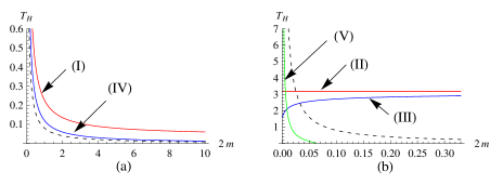
Figure 1: Hawking temperatures of the SBHHMG, (a) for the case of (I) with ${\cal C}=0.5$, $R=0.1~{}({\rm red})$ and (IV) with ${\cal C}=0.5$, $R=0~{}({\rm blue})$, (b) for the case of (II) with ${\cal C}=-1$, $R=10~{}({\rm red})$, (III) with ${\cal C}=-1.5$, $R=10~{}({\rm blue})$, and (V) ${\cal C}=-0.5$, $R=-0.5~{}({\rm green})$. The dashed black line is for the Hawking temperature in massless gravity. Note that the horizontal axis is drawn in the unit of $2m$ in order that the graphs are effectively compared with the one of the Schwarzschild black hole in massless gravity.

IV Entropy of the SBHHMG to all orders in the Planck Length

We begin by considering the SBHHMG found in the previous section as

$$ds^{2}=-f(r)dt^{2}+f^{-1}(r)dr^{2}+r^{2}(d\theta^{2}+\sin^{2}\theta d\phi^{2}),$$ (4.16)

where $f(r)=1-\frac{2m}{r}+2Rr+{\cal C}$. Then, let us consider a free scalar field with a mass $\mu$ in the background described by the solution (4.16), which satisfies the Klein-Gordon equation given by

$$(\Box-\mu^{2})\Phi=\frac{1}{\sqrt{-g}}\partial_{\mu}(\sqrt{-g}g^{\mu\nu}\partial_{\nu}\Phi)-\mu^{2}\Phi=0.$$ (4.17)

Substituting the ansatz of wave function $\Phi(t,r,\theta,\phi)=e^{-i\omega t}\psi(r,{\theta},\phi)$ into Eq. (4.17), we find that the Klein-Gordon equation in the spherical coordinates becomes

$$\partial_{r}^{2}\psi+\left(\frac{f^{\prime}}{f}+\frac{2}{r}\right)\partial_{r}\psi+\frac{1}{f}\left({\frac{1}{r^{2}}}\left[\partial^{2}_{\theta}+{\rm cot}\theta\partial_{\theta}+{\frac{1}{{\rm sin}^{2}\theta}}\partial^{2}_{\phi}\right]+\frac{\omega^{2}}{f}-\mu^{2}\right)\psi=0.$$ (4.18)

Here, the prime denotes the derivative with respect to $r$. By using the Wenzel-Kramers-Brillouin approximation tHooft:1984kcu with $\psi\sim e^{iS(r,\theta,\phi)}$ and keeping the real parts, we have the following modified dispersion relation

$$p_{\mu}p^{\mu}=-\frac{\omega^{2}}{f}+f{p_{r}}^{2}+\frac{p^{2}_{\theta}}{r^{2}}+\frac{p_{\phi}^{2}}{r^{2}{\rm sin}^{2}\theta}=-\mu^{2}$$ (4.19)

where $p_{r}=\frac{\partial S}{\partial r}$, $p_{\theta}=\frac{\partial S}{\partial\theta}$ and $p_{\phi}=\frac{\partial S}{\partial\phi}$. Furthermore, we also obtain the square module of momentum as follows

$$p^{2}\equiv g^{rr}{p_{r}}^{2}+g^{\theta\theta}{p_{\theta}}^{2}+g^{\phi\phi}{p_{\phi}}^{2}=\frac{\omega^{2}}{f}-\mu^{2}.$$ (4.20)

Then, the volume in the momentum phase space is given by

$$V_{p}(r,\theta)=\int dp_{r}dp_{\theta}dp_{\phi}=\frac{4\pi}{3}\frac{r^{2}{\rm sin}\theta}{\sqrt{f}}\left(\frac{\omega^{2}}{f}-\mu^{2}\right)^{\frac{3}{2}}$$ (4.21)

with the condition $\omega\geq\mu\sqrt{f}$.

Now, let us calculate the statistical entropy of the scalar field on the SBHHMG by imposing the additional GUP effect to all orders in the Planck length units. When the gravity is turned on, the number of quantum states in a volume element in phase cell space based on the GUP in (3+1)-dimensions is given by

$$dn_{A}=\frac{d^{3}xd^{3}p}{(2\pi)^{3}}e^{-\lambda p^{2}},$$ (4.22)

where $p^{2}$ is given in Eq. (4.20) and one quantum state corresponding to a cell of volume is changed from $(2\pi)^{3}$ into $(2\pi)^{3}e^{\lambda p^{2}}$ in the phase space Li:2002xb ; Zhao:2003eu ; Liu:2004xh ; Kim:2006rx . Here, the subscript $A$ denotes the quantity for all orders in the Planck length. Note that in the limit of $\lambda\rightarrow 0$, we have the number of quantum states with HUP tHooft:1984kcu . From Eqs. (4.20) and (4.22), the number of quantum states related to the radial mode with energy less than $\omega$ is given by

$$n_{A}(\omega)=\frac{2}{3\pi}\int_{r_{+}}dr\frac{r^{2}}{\sqrt{f}}\left(\frac{{\omega}^{2}}{f}-\mu^{2}\right)^{\frac{3}{2}}e^{-\lambda(\frac{{\omega}^{2}}{f}-\mu^{2})}.$$ (4.23)

It is interesting to note that $n_{A}(\omega)$ is convergent at the horizon without any artificial cutoff because of the existence of the suppressing exponential $\lambda$-term induced from the GUP.

For the bosonic case, the free energy of a thermal ensemble of scalar fields at inverse temperature $\beta$ is given by

$$F_{A} = \frac{1}{\beta}\sum_{K}\ln\left(1-e^{-\beta\omega_{K}}\right)$$ (4.24)

$$= -\frac{2}{3\pi}\int_{r_{+}}dr\frac{r^{2}}{\sqrt{f}}\int^{\infty}_{\mu\sqrt{f}}d\omega~{}\frac{\left(\frac{{\omega}^{2}}{f}-\mu^{2}\right)^{\frac{3}{2}}}{e^{\beta\omega}-1}e^{-\lambda(\frac{{\omega}^{2}}{f}-\mu^{2})}.$$

Here, we have considered the continuum limit, integrated it by parts and used the number of quantum states (4.23).

Now, we are only interested in the contribution from just the vicinity near the event horizon in the range of $(r_{+},r_{+}+\epsilon)$ where $\epsilon$ is the brick wall cutoff used to remove ultraviolet divergences. Since $f\rightarrow 0$ near the event horizon, $\frac{{\omega}^{2}}{f}-\mu^{2}$ becomes $\frac{{\omega}^{2}}{f}$ so that we do not need to require the little mass approximation. Then, the free energy can be rewritten as

$$F_{A}=-\frac{2}{3\pi}\int^{r_{+}+\epsilon}_{r_{+}}dr\frac{r^{2}}{f^{2}}\int^{\infty}_{0}d\omega\frac{{\omega}^{3}}{e^{\beta\omega}-1}e^{-\lambda{\frac{{\omega}^{2}}{f}}}.$$ (4.25)

On the other hand, the minimal length (2.4) is related to a proper distance of $\epsilon$ order as

$$(\Delta x)_{\rm min}=\sqrt{\frac{e\lambda}{2}}\equiv\int_{r_{+}}^{r_{+}+\epsilon}\frac{dr}{\sqrt{f(r)}}\approx\int_{r_{+}}^{r_{+}+\epsilon}\frac{dr}{\sqrt{2\kappa_{+}(r-r_{+})}}=\sqrt{\frac{2\epsilon}{\kappa_{+}}},$$ (4.26)

where the metric function $f(r)$ is expanded near the event horizon as

$$f(r)\approx f(r_{+})+2\kappa_{+}(r-r_{+})+{\cal O}\left((r-r_{+})^{2}\right),$$ (4.27)

and in the second term $\frac{1}{2}\frac{df}{dr}|_{r=r_{+}}$ is replaced by the surface gravity $\kappa_{+}$ (3.14). Thus, one can use the minimal length as a natural ultraviolet cutoff, which shall provide a convergent entropy integral.

Then, from $F_{A}$ in Eq. (4.25), one can find the entropy as

$$S_{A} = \beta^{2}\frac{\partial F_{A}}{\partial\beta}\mid_{\beta=\beta_{+}}$$ (4.28)

$$= \frac{\beta^{2}_{+}}{6\pi}\int^{r_{+}+\epsilon}_{r_{+}}dr\frac{r^{2}}{f^{2}}\int^{\infty}_{0}d\omega\frac{{\omega}^{4}}{\sinh^{2}(\frac{\beta_{+}}{2}\omega)}e^{-\lambda{\frac{{\omega}^{2}}{f}}}.$$

By defining $x\equiv\sqrt{\lambda}\omega$, this can be recast by

$$S_{A}=\frac{\beta^{2}_{+}}{6\pi\lambda^{2}\sqrt{\lambda}}\int^{\infty}_{0}dx\frac{{x}^{4}}{\sinh^{2}(\frac{\beta_{+}}{2\sqrt{\lambda}}x)}\Lambda(x,\epsilon),$$ (4.29)

where

$$\Lambda(x,\epsilon)\equiv\int^{r_{+}+\epsilon}_{r_{+}}dr~{}\frac{r^{2}}{f^{2}}~{}e^{-\frac{x^{2}}{f}}.$$ (4.30)

Now, in order to find a final expression of entropy, one needs to perform proper integrations of Eqs. (4.29) and (4.30), which are depending on both metric functions and types of the GUP. In Kim:2007if , we had calculated this by expanding all the functions only to the leading order near the horizon. However, in this work, we would integrate Eqs. (4.29) and (4.30) by the substitution method, which will give us next order correction terms to the entropy. First of all, near the horizon, we expand Eq. (4.30) as

$$\Lambda(x,\epsilon)\approx\int^{r_{+}+\epsilon}_{r_{+}}dr~{}\frac{r^{2}}{[2\kappa_{+}(r-r_{+})]^{2}}~{}e^{-\frac{x^{2}}{2\kappa_{+}(r-r_{+})}}.$$ (4.31)

This can be integrated by the substitution of $t=x^{2}/2\kappa_{+}(r-r_{+})$ in an exact and closed form as

$$\Lambda(x,\epsilon) = \frac{1}{2\kappa_{+}x^{2}}\int^{\infty}_{\frac{x^{2}}{2\kappa_{+}\epsilon}}dt\left(r^{2}_{+}+\frac{r_{+}x^{2}}{\kappa_{+}t}+\frac{x^{4}}{4\kappa^{2}_{+}t^{2}}\right)e^{-t}$$ (4.32)

$$= \frac{r^{2}_{+}}{2\kappa_{+}x^{2}}\Gamma(1,\frac{x^{2}}{2\kappa_{+}\epsilon})+\frac{r_{+}}{2\kappa^{2}_{+}}\Gamma(0,\frac{x^{2}}{2\kappa_{+}\epsilon})+\frac{x^{2}}{8\kappa^{3}_{+}}\Gamma(-1,\frac{x^{2}}{2\kappa_{+}\epsilon}),$$

where we have used the incomplete Gamma function given by

$$\Gamma(a,z)=\int^{\infty}_{z}dt~{}t^{a-1}e^{-t}.$$ (4.33)

The incomplete Gamma function was also used in efficiently finding the entropy for the noncommutative acoustic black hole Anacleto:2014apa .

Then, all order GUP corrected entropy can be written as

$$S_{A}=\frac{\beta^{2}_{+}r^{2}_{+}}{12\pi\lambda^{2}\sqrt{\lambda}\kappa_{+}}\int^{\infty}_{0}dx\frac{{x}^{2}\Gamma(1,\frac{x^{2}}{2\kappa_{+}\epsilon})}{\sinh^{2}(\frac{\beta_{+}x}{2\sqrt{\lambda}})}+\frac{\beta^{2}_{+}r_{+}}{12\pi\lambda^{2}\sqrt{\lambda}\kappa^{2}_{+}}\int^{\infty}_{0}dx\frac{{x}^{4}\Gamma(0,\frac{x^{2}}{2\kappa_{+}\epsilon})}{\sinh^{2}(\frac{\beta_{+}x}{2\sqrt{\lambda}})}+\frac{\beta^{2}_{+}}{48\pi\lambda^{2}\sqrt{\lambda}\kappa^{3}_{+}}\int^{\infty}_{0}dx\frac{{x}^{6}\Gamma(-1,\frac{x^{2}}{2\kappa_{+}\epsilon})}{\sinh^{2}(\frac{\beta_{+}x}{2\sqrt{\lambda}})}.$$

Now, by redefining $y\equiv\frac{\beta_{+}x}{2\sqrt{\lambda}}$ and making use of the minimum length (4.26) with $\beta_{+}\kappa_{+}=2\pi$, we have

$$S_{A}=\frac{r^{2}_{+}}{3\pi^{2}\lambda}\int^{\infty}_{0}dy\frac{{y}^{2}\Gamma(1,\frac{2y^{2}}{\pi^{2}e})}{\sinh^{2}y}+\frac{r_{+}\kappa_{+}}{3\pi^{4}}\int^{\infty}_{0}dy\frac{{y}^{4}\Gamma(0,\frac{2y^{2}}{\pi^{2}e})}{\sinh^{2}y}+\frac{\lambda\kappa^{2}_{+}}{12\pi^{6}}\int^{\infty}_{0}dy\frac{{y}^{6}\Gamma(-1,\frac{2y^{2}}{\pi^{2}e})}{\sinh^{2}y}.$$ (4.35)

The integrals can be numerically integrated as

$$\delta_{1} \equiv \int^{\infty}_{0}dy\frac{{y}^{2}\Gamma(1,\frac{2y^{2}}{\pi^{2}e})}{\sinh^{2}y}\approx 1.4509,$$ (4.36)

$$\delta_{2} \equiv \int^{\infty}_{0}dy\frac{{y}^{4}\Gamma(0,\frac{2y^{2}}{\pi^{2}e})}{\sinh^{2}y}\approx 3.0709,$$ (4.37)

$$\delta_{3} \equiv \int^{\infty}_{0}dy\frac{{y}^{6}\Gamma(-1,\frac{2y^{2}}{\pi^{2}e})}{\sinh^{2}y}\approx 18.4609$$ (4.38)

so that the entropy can be obtained as

$$S_{A}=\frac{\delta_{1}}{3\pi^{3}}\lambda^{-1}\left(\frac{A}{4}\right)+\frac{\delta_{2}}{3\pi^{4}}r_{+}\kappa_{+}+\frac{\delta_{3}}{12\pi^{6}}\lambda\kappa^{2}_{+}.$$ (4.39)

Here, $A=4\pi r^{2}_{+}$ is the surface area at the event horizon of the SBHHMG. When we choose the GUP parameter $\lambda$ as

$$\lambda=\frac{\delta_{1}}{3\pi^{3}}\approx 0.0156,$$ (4.40)

we can finally obtain the entropy as

$$S_{A}=\frac{A}{4}+\alpha r_{+}\kappa_{+}+\beta\lambda\kappa^{2}_{+},$$ (4.41)

where

$$\alpha=\frac{\delta_{2}}{3\pi^{4}}\approx 0.0105,~{}~{}~{}\beta\lambda=\frac{\delta_{1}\delta_{3}}{36\pi^{9}}\approx 2.4959\times 10^{-5}.$$ (4.42)

As a result, we have finally obtained the entropy satisfying the area law with correction terms, which are proportional to the surface gravity. It is important to comment that massive graviton effect is included in the event horizon $r_{+}$ through $R$ and $\cal C$.

It seems appropriate to comment on the GUP parameter $\lambda$ and minimum length at this stage. As seen in Table 3, the GUP parameter $\lambda$ for the all order GUP corrected $S_{A}$ is the smallest among other parameters which are for the leading order GUP corrected $S_{L}$ based on (2.2) and the all order GUP corrected $S^{\rm old}_{A}$ with the leading order approximation Kim:2007if . On the other hand, the all order GUP corrected $S_{A}$ has the smallest minimal length and thinnest cutoff $\epsilon$. Note that in the all order GUP corrected $S_{A}$ the first term is the same with the leading order approximation in Kim:2007if . However, it also includes next higher order contributions expressed in Eq. (4.36). Moreover, by considering the integration using the substitution method, we have obtained the all order GUP corrected entropy with next orders of correction.

Table 3: Entropy, GUP parameter and minimal length. Note that the ellipses in the entropy are for next order terms and $\kappa_{H}$ in the last row is for the surface gravity in massless gravity.

	entropy	GUP parameter	minimal length	$\epsilon$
all order GUP correction in SBHHMG	$S_{A}=\frac{\delta_{1}}{3\pi^{3}\lambda}\left(\frac{A}{4}\right)+\cdot\cdot\cdot$	$\lambda=\frac{\delta_{1}}{3\pi^{3}}=0.0156$	$(\Delta x)_{\rm min}=\sqrt{e\lambda/2}=0.1456$	$\frac{e}{4}\lambda\kappa_{+}$
leading order GUP correction in SBHHMG	$S_{L}=\frac{\zeta(3)}{3\pi\lambda}\left(\frac{A}{4}\right)$	$\lambda=\frac{\zeta(3)}{3\pi}=0.1275$	$(\Delta x)^{\rm Kemph}_{\rm min}=2\sqrt{\lambda}=0.4163$	$2\lambda\kappa_{+}$
all order GUP correction in massless gravity	$S^{\rm old}_{A}=\frac{e^{2}\zeta(3)}{2\pi\lambda}\left(\frac{A}{4}\right)+\cdot\cdot\cdot$	$\lambda=\frac{e^{2}\zeta(3)}{2\pi}=1.4136$	$(\Delta x)_{\rm min}=\sqrt{e\lambda/2}=1.3861$	$\frac{e}{4}\lambda\kappa_{H}$

Now, in order to figure out the physical meaning of the all order GUP corrected entropy, let us rearrange the terms making use of the surface gravity (3.14). Then, the modified entropy in the holographic massive gravity can be rewritten as

$$S_{A} = S^{{\rm HUP},\tilde{0}}+S^{{\rm GUP},\tilde{0}}+S^{{\rm GUP},\tilde{m}},$$ (4.43)

where

$$S^{{\rm HUP},\tilde{0}} = \pi r^{2}_{+},$$ (4.44)

$$S^{{\rm GUP},\tilde{0}} = \frac{\alpha}{2}+\frac{\beta\lambda}{4r^{2}_{+}},$$ (4.45)

$$S^{{\rm GUP},\tilde{m}} = {\cal C}\left[\frac{\alpha}{2}+\frac{\beta\lambda}{4r^{2}_{+}}(2+{\cal C})\right]+2R\left[2\beta\lambda R+\alpha r_{+}+\frac{\beta\lambda(1+{\cal C})}{r_{+}}\right].$$ (4.46)

Here, $S^{{\rm HUP},\tilde{0}}$ shows the area’s law of entropy with HUP in the holographic massive gravity. Also, $S^{{\rm GUP},\tilde{0}}$ is the extension of all order GUP corrected entropy in massless gravity Kim:2007if to the holographic massive gravity. Finally, $S^{{\rm GUP},\tilde{m}}$ has new contribution to entropy of the holographic massive gravity. In the massless limit of $R\rightarrow 0$ and ${\cal C}\rightarrow 0$, the all order GUP corrected entropy is reduced to

$$S_{A}=S^{{\rm HUP},0}+S^{{\rm GUP},0},$$ (4.47)

where

$$S^{{\rm HUP},0} = \pi(2m)^{2},$$ (4.48)

$$S^{{\rm GUP},0} = \frac{\alpha}{2}+\frac{\beta\lambda}{4(2m)^{2}}.$$ (4.49)

Note that $2m$ is the radius of the event horizon and $S^{{\rm GUP},\tilde{m}}=0$ in the massless limit. On the other hand, by turning off the all order GUP correction to entropy in Eq. (4.43), we have

$$S_{A}=\pi r^{2}_{+},$$ (4.50)

which is the area’s law of the Schwarzschild black hole without the GUP.

In Fig. 2, we have drawn the entropy of the Schwarzschild black hole in the massless/holographic massive gravity with HUP/GUP. In Fig. 2(a), the dashed line is for the entropy of the Schwarzschild black hole in massless gravity with HUP, which is increasing with $\pi(2m)^{2}$. When we turn on the massive gravitons, the ares’s law increasing with $\pi(2m)^{2}$ is changed to $\pi r^{2}_{+}$ since $r_{+}$ is the event horizon in the holographic massive gravity. This is represented by the solid line in Fig. 2(a). On the other hand, the dashed line in Fig. 2(b) is for the entropy of the Schwarzschild black hole in massless gravity with all order corrected GUP, while the solid is for the entropy of the Schwarzschild black hole in holographic massive gravity with all order corrected GUP. As shown in the figure, the all order GUP correction makes the entropies divergent near $m=0$, which was predicted in loop quantum gravity Domagala:2004jt ; Meissner:2004ju . Note that the gaps between the curves come from the gravitons in the holographic massive gravity.

In Fig. 3, we have drawn the all order GUP corrected entropy of the SBHHMG by varying $R$ and ${\cal C}$. Fig. 3(a) is drawn by varying ${\cal C}$ with a fixed $R$, while in Fig. 3(b), by varying $R$ with a fixed ${\cal C}$, respectively. These figures all show results that near $m=0$ all order GUP corrections give dominant effects on the generalized Bekenstein-Hawking entropy.

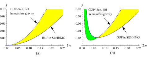
Figure 2: Entropy of the Schwarzschild black hole in the massless and holographic massive gravity with HUP/GUP: (a) the dashed line is for the Schwarzschild black hole in massless gravity with HUP ($\alpha$, $\beta$, $R$, ${\cal C}=0$) and the solid line is for the SBHHMG with HUP ($\alpha$, $\beta=0$, $R=0.1$, ${\cal C}=0.5$), and (b) the dashed line is for the Schwarzschild black hole in massless gravity with all order corrected GUP ($\alpha$, $\beta\neq 0$, $R$, ${\cal C}=0$) and the solid line is for the SBHHMG with all order corrected GUP ($\alpha$, $\beta\neq 0$, $R=0.1$, ${\cal C}=0.5$). Note that the gaps between the curves come from the gravitons in the holographic massive gravity. Here, $\alpha$, $\beta$ are given by Eq. (4.42), respectively.

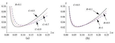
Figure 3: Entropy of the SBHHMG: (a) by varying ${\cal C}=-0.5,~{}0,~{}0.5$ with a fixed $R=0.1$ and (b) by varying $R=0.1,~{}0.5,~{}1$ with a fixed ${\cal C}=0.5$.

V Summary and Discussion

In this paper, we have studied the Hawking temperature and entropy of a scalar field on the Schwarzschild black hole in the holographic massive gravity. This is an modification of the Schwarzschild black hole to have nonzero mass of gravitons. At the same time, we have studied the effect of a GUP to all orders in Planck length units to the SBHHMG where a GUP admits a minimal length at the quantum level and induces quantitative corrections to the thermodynamic quantities. As a result, we have found the spherically symmetric Schwarzschild black hole solution with massive gravitons represented by $R$ and ${\cal C}$ which contribute linear and constant terms to the solution, respectively. The allowed event horizons are then classified by relative magnitudes of $R$ and ${\cal C}$, and even no event horizon exists when $R<-(1+{\cal C})^{2}/16m$. We have also obtained the Schwarzschild-like Hawking temperatures when $R\geq 0$ and ${\cal C}>-1$, and some bizarre ones in the other ranges of $R$ and ${\cal C}$. Thus, one can see that the modified Schwarzschild black hole provided by the massive gravity and the GUP as a quantum correction is only possible when $R\geq 0$ and ${\cal C}>-1$. On the other hand, we have calculated the statistical entropy by carefully counting the number of the GUP induced quantum states in the just vicinity near the horizon. This modification of state density is due to the GUP where the momentum is a subject of a modification in the momentum space representation. Comparing with the previous calculations without massive gravitons Li:2002xb ; Zhao:2003eu ; Liu:2004xh ; Kim:2006rx ; Yoon:2007aj ; Hossenfelder:2006cw ; Hossenfelder:2005ed ; Nouicer:2007jg ; Nouicer:2007cw ; Kim:2007if where many authors have expanded the relevant functions only to the lowest order, we have made use of the substitution method of integral and finally obtained not only the generalized Bekenstein-Hawking entropy of the SBHHMG to all orders in the Planck length units, but also new additional correction terms, which are proportional to surface gravity. Moreover, we have shown that the all order GUP corrected entropy obtained in this paper has the smallest GUP parameter $\lambda$, minimal length, and thinnest cutoff $\epsilon$, compared with the previous results Zhao:2003eu ; Liu:2004xh ; Kim:2006rx ; Yoon:2007aj ; Nouicer:2007jg ; Nouicer:2007cw ; Kim:2007if . Furthermore, we have also found that all order GUP corrections to the Bekenstein-Hawking entropy both in massless and massive gravities give dominant effects near $m=0$. As a final remark, while our results are obtained based on the existence of the event horizons, it would also be interesting to study further the no-horizon ranges of the massive parameters in Table 1 which might have implications on the information loss problem Singleton:2010gz ; Eune:2014tea as producing dark stars on a horizonless background Kawai:2013mda ; Ho:2015vga .

- (1) G. Amelino-Camelia, Living Rev. Rel. 16, 5 (2013) [arXiv:0806.0339 [gr-qc]].
- (2) M. Fierz and W. Pauli, Proc. Roy. Soc. Lond. A 173, 211 (1939).
- (3) D. G. Boulware and S. Deser, Phys. Rev. D 6, 3368 (1972).
- (4) H. van Dam and M. J. G. Veltman, Nucl. Phys. B 22, 397 (1970).
- (5) V. I. Zakharov, JETP Lett. 12, 312 (1970).
- (6) A. I. Vainshtein, Phys. Lett. B 39, 393 (1972).
- (7) C. de Rham and G. Gabadadze, Phys. Rev. D 82, 044020 (2010) [arXiv:1007.0443 [hep-th]].
- (8) C. de Rham, G. Gabadadze and A. J. Tolley, Phys. Rev. Lett. 106, 231101 (2011) [arXiv:1011.1232 [hep-th]].
- (9) S. F. Hassan and R. A. Rosen, Phys. Rev. Lett. 108, 041101 (2012) [arXiv:1106.3344 [hep-th]].
- (10) S. F. Hassan, R. A. Rosen and A. Schmidt-May, JHEP 1202, 026 (2012) [arXiv:1109.3230 [hep-th]].
- (11) J. Kluson, JHEP 01, 013 (2012) [arXiv:1109.3052 [hep-th]].
- (12) J. Kluson, JHEP 06, 170 (2012) [arXiv:1112.5267 [hep-th]].
- (13) J. Kluson, Phys. Rev. D 86, 124005 (2012) [arXiv:1202.5899 [hep-th]].
- (14) D. Comelli, M. Crisostomi, F. Nesti and L. Pilo, Phys. Rev. D 86, 101502(R) (2012) [arXiv:1204.1027 [hep-th]].
- (15) A. Golovnev, Phys. Lett. B 707, 404 (2012) [arXiv:1112.2134 [gr-qc]].
- (16) C. Deffayet, J. Mourad and G. Zahariade, JCAP 01, 032 (2013) [arXiv:1207.6338 [hep-th]].
- (17) D. Vegh, arXiv:1301.0537 [hep-th].
- (18) R. A. Davison, Phys. Rev. D 88, 086003 (2013) [arXiv:1306.5792 [hep-th]].
- (19) M. Blake and D. Tong, Phys. Rev. D 88, 106004 (2013) [arXiv:1308.4970 [hep-th]].
- (20) M. Blake, D. Tong and D. Vegh, Phys. Rev. Lett. 112, 071602 (2014) [arXiv:1310.3832 [hep-th]].
- (21) R. G. Cai, Y. P. Hu, Q. Y. Pan and Y. L. Zhang, Phys. Rev. D 91, 024032 (2015) [arXiv:1409.2369 [hep-th]].
- (22) A. Adams, D. A. Roberts and O. Saremi, Phys. Rev. D 91, 046003 (2015) [arXiv:1408.6560 [hep-th]].
- (23) S. H. Hendi, S. Panahiyan and B. Eslam Panah, JHEP 1601, 129 (2016) [arXiv:1507.06563 [hep-th]].
- (24) Y. P. Hu, X. M. Wu and H. Zhang, Phys. Rev. D 95, 084002 (2017) [arXiv:1611.09042 [gr-qc]].
- (25) D. C. Zou, R. Yue and M. Zhang, Eur. Phys. J. C 77, 256 (2017) [arXiv:1612.08056 [gr-qc]].
- (26) S. H. Hendi, R. B. Mann, S. Panahiyan and B. Eslam Panah, Phys. Rev. D 95, 021501(R) (2017) [arXiv:1702.00432 [gr-qc]].
- (27) L. Tannukij, P. Wongjun and S. G. Ghosh, Eur. Phys. J. C 77, 846 (2017) [arXiv:1701.05332 [gr-qc]].
- (28) S. H. Hendi, B. Eslam Panah, S. Panahiyan, H. Liu and X.-H. Meng, Phys. Lett. B 781, 40 (2018) [arXiv:1707.02231 [hep-th]].
- (29) S. H. Hendi and A. Dehghani, Eur. Phys. J. C 79, 227 (2019) [arXiv:1811.01018 [gr-qc]].
- (30) M. Chabab, H. El Moumni, S. Iraoui and K. Masmar, Eur. Phys. J. C 79, 342 (2019) [arXiv:1904.03532 [hep-th]].
- (31) S. T. Hong, Y. W. Kim and Y. J. Park, Phys. Rev. D 99, 024047 (2019) [arXiv:1812.00373 [gr-qc]].
- (32) S. T. Hong, Y. W. Kim and Y. J. Park, Phys. Lett. B 800, 135116 (2020) [arXiv:1905.04860 [gr-qc]].
- (33) A. Kempf, G. Mangano and R. B. Mann, Phys. Rev. D 52, 1108 (1995) [arXiv:hep-th/9412167 [hep-th]].
- (34) L. J. Garay, Int. J. Mod. Phys. A 10, 145 (1995) [arXiv:gr-qc/9403008 [gr-qc]].
- (35) F. Scardigli, Phys. Lett. B 452, 39 (1999) [arXiv:hep-th/9904025 [hep-th]].
- (36) S. Kalyana Rama, Phys. Lett. B 519, 103 (2001) [arXiv:hep-th/0107255 [hep-th]].
- (37) L. N. Chang, D. Minic, N. Okamura and T. Takeuchi, Phys. Rev. D 65, 125028 (2002) [arXiv:hep-th/0201017 [hep-th]].
- (38) S. Hossenfelder, Living Rev. Rel. 16, 2 (2013) [arXiv:1203.6191 [gr-qc]].
- (39) R. J. Adler, P. Chen and D. I. Santiago, Gen. Rel. Grav. 33, 2101 (2001) [arXiv:gr-qc/0106080 [gr-qc]].
- (40) F. Scardigli and R. Casadio, Class. Quant. Grav. 20, 3915 (2003) [arXiv:hep-th/0307174 [hep-th]].
- (41) M. R. Setare, Phys. Rev. D 70, 087501 (2004) [arXiv:hep-th/0410044 [hep-th]].
- (42) A. J. M. Medved and E. C. Vagenas, Phys. Rev. D 70, 124021 (2004) [arXiv:hep-th/0411022 [hep-th]].
- (43) Y. Ling, B. Hu and X. Li, Phys. Rev. D 73, 087702 (2006) [arXiv:gr-qc/0512083 [gr-qc]].
- (44) Y. S. Myung, Y. W. Kim and Y. J. Park, Phys. Lett. B 645, 393 (2007) [arXiv:gr-qc/0609031 [gr-qc]].
- (45) Y. W. Kim, S. K. Kim and Y. J. Park, Eur. Phys. J. C 76, 557 (2016) [arXiv:1607.06185 [gr-qc]].
- (46) Z. W. Feng, X. Zhou and S. Q. Zhou, [arXiv:2008.01661 [gr-qc]].
- (47) J. D. Bekenstein, Lett. Nuovo Cim. 4, 737 (1972).
- (48) J. D. Bekenstein, Phys. Rev. D 7, 2333 (1973).
- (49) J. D. Bekenstein, Phys. Rev. D 9, 3292 (1974).
- (50) S. W. Hawking, Nature 248, 30-31 (1974)
- (51) S. W. Hawking, Commun. Math. Phys. 43, 199 (1975) [erratum: Commun. Math. Phys. 46, 206 (1976)].
- (52) G. ’t Hooft, Nucl. Phys. B 256, 727 (1985).
- (53) R. B. Mann, L. Tarasov and A. Zelnikov, Class. Quant. Grav. 9, 1487 (1992).
- (54) A. Ghosh and P. Mitra, Phys. Rev. Lett. 73, 2521 (1994) [arXiv:hep-th/9406210 [hep-th]].
- (55) J. G. Demers, R. Lafrance and R. C. Myers, Phys. Rev. D 52, 2245 (1995). [arXiv:gr-qc/9503003 [gr-qc]].
- (56) R. G. Cai and Y. Z. Zhang, Mod. Phys. Lett. A 11, 2027 (1996).
- (57) S. W. Kim, W. T. Kim, Y. J. Park and H. Shin, Phys. Lett. B 392, 311 (1997) [arXiv:hep-th/9603043 [hep-th]].
- (58) S. P. Kim, S. K. Kim, K. S. Soh and J. H. Yee, Phys. Rev. D 55, 2159 (1997) [arXiv:gr-qc/9608015 [gr-qc]].
- (59) J. Ho, W. T. Kim, Y. J. Park and H. Shin, Class. Quant. Grav. 14, 2617 (1997) [arXiv:gr-qc/9704032 [gr-qc]].
- (60) S. Mukohyama and W. Israel, Phys. Rev. D 58, 104005 (1998) [arXiv:gr-qc/9806012 [gr-qc]].
- (61) J. L. Jing and M. L. Yan, Phys. Rev. D 60, 084015 (1999) [arXiv:gr-qc/9904001 [gr-qc]].
- (62) L. Xiang and Z. Zheng, Phys. Rev. D 62, 104001 (2000).
- (63) E. Winstanley, Phys. Rev. D 63, 084013 (2001) [arXiv:hep-th/0011176 [hep-th]].
- (64) W. T. Kim, J. J. Oh and Y. J. Park, Phys. Lett. B 512, 131 (2001) [arXiv:hep-th/0103147 [hep-th]].
- (65) A. J. M. Medved, Class. Quant. Grav. 19, 405 (2002) [arXiv:hep-th/0110118 [hep-th]].
- (66) C. J. Gao and Y. G. Shen, Phys. Rev. D 65, 084043 (2002).
- (67) X. F. Sun and W. B. Liu, Mod. Phys. Lett. A 19, 677 (2004).
- (68) M. Kenmoku, K. Ishimoto, K. K. Nandi and K. Shigemoto, Phys. Rev. D 73, 064004 (2006) [arXiv:gr-qc/0510012 [gr-qc]].
- (69) S. Sarkar, S. Shankaranarayanan and L. Sriramkumar, Phys. Rev. D 78, 024003 (2008) [arXiv:0710.2013 [gr-qc]].
- (70) D. Singleton, E. C. Vagenas, T. Zhu and J. R. Ren, JHEP 08, 089 (2010) [erratum: JHEP 01, 021 (2011)] [arXiv:1005.3778 [gr-qc]].
- (71) M. Eune and W. Kim, Phys. Lett. B 723, 177 (2013) [arXiv:1211.2048 [gr-qc]].
- (72) F. Lenz, K. Ohta and K. Yazaki, Phys. Rev. D 92,064018 (2015) [arXiv:1402.6142 [hep-th]].
- (73) M. Eune, Y. Gim and W. Kim, Phys. Rev. D 91, 044037 (2015) [arXiv:1409.5548 [gr-qc]].
- (74) A. D. Kamali, H. Shababi and K. Nozari, Int. J. Mod. Phys. A 31, 1650160 (2016).
- (75) A. D. Kamali and H. Shababi, Adv. High Energy Phys. 2018, 3936169 (2018).
- (76) E. C. Vagenas, A. F. Ali, M. Hemeda and H. Alshal, Eur. Phys. J. C 79, 398 (2019) [arXiv:1903.08494 [hep-th]].
- (77) B. Cuadros-Melgar, R. D. B. Fontana and J. de Oliveira, Eur. Phys. J. C 80, 848 (2020) [arXiv:2003.00564 [gr-qc]].
- (78) X. Li, Phys. Lett. B 540, 9 (2002) [arXiv:gr-qc/0204029 [gr-qc]].
- (79) R. Zhao, Y. Q. Wu and L. C. Zhang, Class. Quant. Grav. 20, 4885 (2003).
- (80) C. Z. Liu, X. Li and Z. Zhao, Gen. Rel. Grav. 36, 1135 (2004).
- (81) W. Kim, Y. W. Kim and Y. J. Park, Phys. Rev. D 74, 104001 (2006) [arXiv:gr-qc/0605084 [gr-qc]].
- (82) M. Yoon, J. Ha and W. Kim, Phys. Rev. D 76, 047501 (2007) [arXiv:0706.0364 [gr-qc]].
- (83) S. Hossenfelder, Phys. Rev. D 73, 105013 (2006) [arXiv:hep-th/0603032 [hep-th]].
- (84) S. Hossenfelder, Class. Quant. Grav. 23, 1815 (2006) [arXiv:hep-th/0510245 [hep-th]].
- (85) K. Nouicer, Phys. Lett. B 646, 63 (2007) [arXiv:0704.1261 [gr-qc]].
- (86) K. Nouicer, Class. Quant. Grav. 25, 075010 (2008) [arXiv:0705.2733 [gr-qc]].
- (87) Y. W. Kim and Y. J. Park, Phys. Lett. B 655, 172 (2007) [arXiv:0707.2128 [gr-qc]].
- (88) A. Smailagic and E. Spallucci, J. Phys. A 36, L467 (2003) [arXiv:hep-th/0307217 [hep-th]].
- (89) A. Smailagic and E. Spallucci, J. Phys. A 36, L517 (2003) [arXiv:hep-th/0308193 [hep-th]].
- (90) K. Nouicer and M. Debbabi, Phys. Lett. A 361, 305 (2007).
- (91) R. M. Corless, G. H. Gonnet, D. E. G. Hare, D. J. Jeffrey and D. E. Knuth, Adv. Comput. Math. 5, 329 (1996).
- (92) R. M. Wald, General Relativity (University of Chicago, Chicago, 1984).
- (93) M. A. Anacleto, F. A. Brito, E. Passos and W. P. Santos, Phys. Lett. B 737, 6 (2014) [arXiv:1405.2046 [hep-th]].
- (94) M. Domagala and J. Lewandowski, Class. Quant. Grav. 21, 5233 (2004) [arXiv:gr-qc/0407051 [gr-qc]].
- (95) K. A. Meissner, Class. Quant. Grav. 21, 5245 (2004) [arXiv:gr-qc/0407052 [gr-qc]].
- (96) H. Kawai, Y. Matsuo and Y. Yokokura, Int. J. Mod. Phys. A 28, 1350050 (2013) [arXiv:1302.4733 [hep-th]].
- (97) P. M. Ho, Nucl. Phys. B 909, 394 (2016) [arXiv:1510.07157 [hep-th]].