Non-asymptotic Confidence Intervals of Off-policy Evaluation: Primal and Dual Bounds

Abstract

Off-policy evaluation (OPE) is the task of estimating the expected reward of a given policy based on offline data previously collected under different policies. Therefore, OPE is a key step in applying reinforcement learning to real-world domains such as medical treatment, where interactive data collection is expensive or even unsafe. As the observed data tends to be noisy and limited, it is essential to provide rigorous uncertainty quantification, not just a point estimation, when applying OPE to make high stakes decisions. This work considers the problem of constructing non-asymptotic confidence intervals in infinite-horizon off-policy evaluation, which remains a challenging open question. We develop a practical algorithm through a primal-dual optimization-based approach, which leverages the kernel Bellman loss (KBL) of Feng et al. (2019) and a new martingale concentration inequality of KBL applicable to time-dependent data with unknown mixing conditions. Our algorithm makes minimum assumptions on the data and the function class of the Q-function, and works for the behavior-agnostic settings where the data is collected under a mix of arbitrary unknown behavior policies. We present empirical results that clearly demonstrate the advantages of our approach over existing methods.

1 Introduction

Off-policy evaluation (OPE) seeks to estimate the expected reward of a target policy in reinforcement learning (RL) from observational data collected under different behavior policies (e.g., Murphy et al., 2001; Fonteneau et al., 2013; Jiang and Li, 2016; Liu et al., 2018a). OPE plays a central role in applying reinforcement learning (RL) with only observational data and has found important applications in areas such as medical treatments, autonomous driving, where interactive “on-policy” data is expensive or even infeasible to collect.

As the observed data is often noisy and limited, applying OPE to assist high-stakes decision-making entails a rigorous, non-asymptotic approach to quantify the uncertainty in the estimation. In this way, the decision makers are informed of the degree of the risk and can avoid the dangerous case of being overconfident in making costly and/or irreversible decisions. This work addresses the uncertainty quantification in OPE by constructing non-asymptotically correct confidence intervals that contains the true expected reward of the target policy with a probability no smaller than a user-specified confidence level.

To date, Off-policy evaluation per se has remained a key technical challenge in the literature (e.g., Precup, 2000; Thomas and Brunskill, 2016; Jiang and Li, 2016; Liu et al., 2018a), let alone gaining rigorous confidence estimation of it. This is especially true when 1) the underlying RL problem is long or infinite horizon (a.k.a. the curse of horizon (Liu et al., 2018a)); and 2) the data is collected under arbitrary and unknown algorithms (a.k.a. behavior-agnostic). In such cases, the collected data can exhibit complex and unknown time-dependency structure, which makes constructing rigorous non-asymptotic confidence bounds particularly challenging. Traditionally, the main approach of deriving non-asymptotic confidence bounds in OPE is to combine importance sampling (IS) with certain concentration inequality (e.g., Thomas et al., 2015a). However, the classical IS-based methods tend to degenerate for long or infinite horizon problems (Liu et al., 2018a, 2020). Moreover, they cannot be applied to the behavior-agnostic settings and also fail to handle the complicated time-dependency structure inside individual trajectories. In fact, the IS-based methods only work for short-horizon problems with a large number of independently collected trajectories drawn under known policies.

In this work, we provide a practical algorithm with theoretical guarantee for Behavior-agnostic, Off-policy, Infinite-horizon, Non-asymptotic, Confidence intervals based on arbitrarily Dependent data (BONDIC). This method is motivated by a recently proposed optimization-based approach to estimating OPE confidence bounds (Feng et al., 2020), which leverages a tail bound of kernel Bellman loss (Feng et al., 2019). Our approach achieves a new dual bound that is both an order-of-magnitude tighter and more computationally efficient than that of Feng et al. (2020). These improvements are based on two pillars: 1) a new primal-dual perspective on the non-asymptotic confidence bounds of infinite-horizon OPE; and 2) a new martingale concentration inequality on the kernel Bellman loss that applies to behavior-agnostic off-policy data with arbitrary time-dependency between transition pairs. Our simple and practical method can provide reliable and informative bounds on a variety of benchmarks.

Outline

The rest of the paper is organized as follows. We introduce the problem setting in Section 2 and discuss related works in Section 3. In Section 4, we give an overview on two dual approaches to infinite-horizon OPE that are closely related to our method (but do not consider non-asymptotic error bounds). We then present a martingale concentration bound for kernel Bellman loss in Section 5, which is used in our main approach described in Section 6. Finally, we perform empirical studies in Section 7. The proofs and additional discussions can be found in Appendix.

2 Background, Data Assumption, Problem Setting

Consider an agent acting in an unknown environment. At each time step $t$, the agent observes the current state $s_{t}$ in a state space $\mathcal{S}$, takes an action $a_{t}\sim\pi(\cdot~{}|~{}s_{t})$ in an action space $\mathcal{A}$ according to a given policy $\pi$; then, the agent receives a reward $r_{t}$ and the state transits to $s_{t}^{\prime}=s_{t+1}$, following an unknown transition/reward distribution $(r_{t},s_{t+1})\sim\mathsf{P}(\cdot~{}|~{}s_{t},a_{t})$. Assume the initial state $s_{0}$ is drawn from an known initial distribution $\mathsf{D}_{0}$. Let $\gamma\in(0,1)$ be a discount factor. In this setting, the expected reward of $\pi$ is defined as

$$J_{*}:=J_{\pi,\mathsf{P}}:=\lim_{H\to+\infty}\mathbb{E}_{\pi,\mathsf{P}}\left[\sum_{t=0}^{H}\gamma^{t}r_{t}~{}|~{}s_{0}\sim\mathsf{D}_{0}\right],$$ (1)

which is the expected total discounted rewards when we execute $\pi$ starting from $\mathsf{D}_{0}$ for $H$ steps. The focus of this work is the infinite-horizon case with $H\to+\infty$, although our method can also be applied to a finite-horizon, time-inhomogeneous problem by converting it into an infinite-horizon and time-homogeneous problem that incorporates time $t$ as a special state variable (Appendix I). The state-action space $\mathcal{S}\times\mathcal{A}$ can be any domain on which we can define a reproducing kernel Hilbert space (RKHS), either discrete or continuous.

Assume the model $\mathsf{P}$ is unknown, but we can observe a set of transition pairs $\hat{\mathsf{D}}_{n}=(s_{i},a_{i},r_{i},s_{i}^{\prime})_{i=1}^{n}$ that obeys $\mathsf{P}$ in that $(r_{i},s_{i}^{\prime})\sim\mathsf{P}(\cdot~{}|~{}s_{i},a_{i})$. The goal is to construct an interval $[\hat{J}^{-}(\hat{\mathsf{D}}_{n}),~{}\hat{J}^{+}(\hat{\mathsf{D}}_{n})]$ based on the observed data such that the probability that it contains the true $J_{*}$ is no smaller than a user-specified confidence level. We consider the challenging case where the data is off-policy, behavior-agnostic, and time-dependent, as formally specified in the following.

Assumption 2.1 (Data Assumption).

Assume the data $\hat{\mathsf{D}}_{n}=(s_{i},a_{i},r_{i},s_{i}^{\prime})_{i=1}^{n}$ is drawn from an unknown joint distribution $\mathsf{D}_{1:n}^{\diamond}$ on $(\mathcal{S}\times\mathcal{A}\times\mathbb{R}\times\mathcal{S})^{n}$ that satisfies

$$\mathsf{D}_{1:n}^{\diamond}(r_{i},s_{i}^{\prime}~{}|~{}s_{i},a_{i};~{}\hat{\mathsf{D}}_{<i})=\mathsf{P}(r_{i},s_{i}^{\prime}~{}|~{}s_{i},a_{i}),~{}~{}~{}~{}~{}\forall i=1,\ldots,n,$$ (2)

where $\hat{\mathsf{D}}_{<i}:=(s_{j},a_{j},r_{j},s_{j}^{\prime})_{j<i}$.

Goal

Given a dataset $\hat{\mathsf{D}}_{n}$, a target policy $\pi$, and a confidence level $\delta\in(0,1)$, we want to construct an interval $[{\hat{J}^{-}}(\hat{\mathsf{D}}_{n}),{\hat{J}^{+}}(\hat{\mathsf{D}}_{n})]\subset\mathbb{R}$, such that

$$\mathrm{Pr}\left(J_{*}\in\left[{\hat{J}^{-}}(\hat{\mathsf{D}}_{n}),~{}~{}{\hat{J}^{+}}(\hat{\mathsf{D}}_{n})\right]\right)\geq 1-\delta,$$ (3)

where $\mathrm{Pr}(\cdot)$ is w.r.t. the randomness of the data $\hat{\mathsf{D}}_{n}$ drawn from the distribution $\mathsf{D}_{1:n}^{\diamond}$.

The data assumption provides a partial specification of the joint distribution $\mathsf{D}_{1:n}^{\diamond}$, which only requires that $(r_{i},s^{\prime}_{i})$ should be generated from $\mathsf{P}(\cdot~{}|~{}s_{i},a_{i})$ given $(s_{i},a_{i})\cup\hat{\mathsf{D}}_{<i}$ at each step, while imposing no constraints on how $(s_{i},a_{i})$ is generated based on $\hat{\mathsf{D}}_{<i}$. This provides great flexibility in terms of the data collection procedure. For example, $\hat{\mathsf{D}}_{n}$ can be either collected from a single MDP governed by an unknown, time-varying, non-Markovian behavior policy (in which case $(s_{i}^{\prime},a_{i}^{\prime})=(s_{i+1},a_{i+1})$), or be a combination of many short MDP segments (in which case $(s_{i}^{\prime},a_{i}^{\prime})$ may not equal $(s_{i+1},a_{i+1})$). Note that this significantly relaxes the data assumptions in recent works (Liu et al., 2018a; Mousavi et al., 2020; Dai et al., 2020), which require $(s_{i},a_{i})_{i=1}^{n}$ to be independent or i.i.d.

Eq (3) is a correctness requirement of the confidence interval. In addition, we also want to make the interval estimation as tight as possible. Specifically, it is desirable that the length $(\hat{J}^{+}(\hat{\mathsf{D}}_{n})-\hat{J}^{-}(\hat{\mathsf{D}}_{n}))$ of the interval vanishes to zero as $n\to\infty$, ideally with a fast converge rate (e.g., $O(n^{-1/2})$). While assumption 2.1 allows us to construct bounds that are correct and non-vacuous, it is too mild to give meaningful a priori bound on the tightness of the interval estimation. For example, under Assumption 2.1, it is possible that the whole dataset is the replication of a single transition pair, i.e., $(s_{i},a_{i},r_{i},s_{i}^{\prime})=(s_{1},a_{1},r_{1},s_{1}^{\prime})$, in which case we cannot have a $1-\delta$ confidence interval whose length vanishes to zero as $n\to\infty$.

A primary advantage of having an interval estimation is that we know a posteriori length of the confidence interval once we construct it, which provides an instance-based uncertainty estimation without making any additional assumption beyond Assumption 2.1. If a stronger assumption is imposed (e.g., $(s_{i},a_{i},r_{i},s_{i}^{\prime})_{i=1}^{n}$ are i.i.d. or weakly dependent in a proper sense for different $i$), we can derive a priori estimation of the convergence rate of the tightness $(\hat{J}^{+}(\hat{\mathsf{D}}_{n})-\hat{J}^{-}(\hat{\mathsf{D}}_{n}))$ for the confidence interval as shown in Section 6.3 and Appendix D.

A crucial fact is that the data assumption above implies a martingale structure on the empirical Bellman residual operator of the Q-function. As we will show in Section 5, this enables us to derive a key concentration inequality underpinning our non-asymptotic confidence bound.

state	action	reward	state-action	next state-action	next state-action + reward
$s_{i}$	$a_{i}$	$r_{i}$	$x_{i}=(s_{i},a_{i})$	$x_{i}^{\prime}=(s_{i}^{\prime},a_{i}^{\prime})$	$y_{i}=(s_{i}^{\prime},a_{i}^{\prime},r_{i})$

Table 1: Summary of the notation. We assume we observe pairs of $(s_{i},a_{i},r_{i},s_{i}^{\prime})$, and for each $i$, we augment the data with the next action $a_{i}^{\prime}$ as part of the algorithm by drawing from $\pi(\cdot~{}|~{}s_{i}^{\prime})$, where $\pi$ is the known target policy. The data assumption in Eq (2) is equivalent to saying that $y_{i}\sim\mathsf{P}_{\pi}(\cdot~{}|~{}x_{i})$; see Eq (4).

Notation

We define a few notations that will simplify the presentation in the rest of work. First of all, to facilitate the definition of the empirical Bellman operator in the sequel (see Section 4.1 and Remark 4.1), we append each $(s_{i},a_{i},r_{i},s_{i}^{\prime})$ with a random action $a_{i}^{\prime}$ drawn from the target policy $\pi(\cdot~{}|~{}s_{i}^{\prime})$ following $s_{i}^{\prime}$. This can be done for free as long as the target policy $\pi$ is given. Also, we write $x_{i}=(s_{i},a_{i})$, $x_{i}^{\prime}=(s_{i}^{\prime},a_{i}^{\prime})$, and $y_{i}=(x_{i}^{\prime},r_{i})=(s_{i}^{\prime},a_{i}^{\prime},r_{i})$. Correspondingly, define $\mathcal{X}=\mathcal{S}\times\mathcal{A}$ to be the state-action space. Then the observed data can be written as pairs of $\{x_{i},y_{i}\}_{i=1}^{n}$. We equalize the data $\hat{\mathsf{D}}_{n}$ with its empirical measure $\hat{\mathsf{D}}_{n}=\sum_{i=1}^{n}\mathsf{\delta}_{x_{i},y_{i}}/n$, where $\delta$ is the Delta measure. See Table 1. Define

$$\mathsf{P}_{\pi}(y~{}|~{}x)=\mathsf{P}(s^{\prime},r~{}|~{}x)\pi(a^{\prime}~{}|~{}s^{\prime})\,.$$ (4)

Then Assumption 2.1 is equivalent to saying that $y_{i}\sim\mathsf{P}_{\pi}(\cdot~{}|~{}x_{i})$. In this way, our setting can be viewed as a supervised learning problem on $\{x_{i},y_{i}\}$ with an unknown $\mathsf{P}_{\pi}$. The difference is that we are interested in estimating $J_{\pi,\mathsf{P}}$, which is a nonlinear functional of $\mathsf{P}_{\pi}$, rather than the whole model $\mathsf{P}_{\pi}$ (which would yield a model-based method; see discussions in Section 3).

We use the star notation to label quantities that depend on the unknown parameters (such as $J_{*}$), and the hat notation to denote quantities that depend on observed data (such as $\hat{\mathsf{D}}_{n}$ and $\hat{J}^{\pm}(\hat{\mathsf{D}}_{n})$). The prime notation always denotes the next state (such as $s_{i}^{\prime}$).

3 Related Work

We give an overview of different approaches for uncertainty estimation in OPE.

Finite-Horizon Importance Sampling (IS)

Assume the data is collected by rolling out a known behavior policy $\pi_{0}$ up to a trajectory length $T$, then we can estimate the finite horizon reward by changing $\mathbb{E}_{\pi,\mathsf{P}}[\cdot]$ to $\mathbb{E}_{\pi_{0},\mathsf{P}}[\cdot]$ with importance sampling(e.g., Precup et al., 2000; Precup, 2001; Thomas et al., 2015a, b). Taking the trajectory-wise importance sampling as an example, assume we collect a set of independent trajectories $\tau_{i}:=\{s_{t}^{i},a_{t}^{i},r_{t}^{i}\}_{t=0}^{T-1}$, $i=1,\ldots,m$ up to a trajectory length $T$ by unrolling a known behavior policy $\pi_{0}$. When $T$ is large, we can estimate $J_{*}$ by a weighted averaging:

$$\hat{J}^{\rm{IS}}=\frac{1}{m}\sum_{i=1}^{m}(/\tau_{i})J(\tau_{i})\,,~{}~{}~{}~{}~{}\text{where}~{}~{}~{}(/\tau_{i})=\prod_{t=0}^{T-1}\frac{\pi(a_{t}^{i}|s_{t}^{i})}{\pi_{0}(a_{t}^{i}|s_{t}^{i})}\,,~{}~{}~{}~{}~{}J(\tau_{i})=\sum_{t=0}^{T-1}\gamma^{t}r_{t}^{i}\,.$$ (5)

One can construct non-asymptotic confidence bounds based on $\hat{J}^{\rm{IS}}$ using variants of concentration inequalities (Thomas, 2015; Thomas et al., 2015b). Unfortunately, a key problem with this IS estimator is that the importance weight $(/\tau_{i})$ is a product of the density ratios over time, and hence tends to cause an explosion in variance when the trajectory length $T$ is large. Although improvement can be made by using per-step and self-normalized weights (Precup, 2001), or control variates (Jiang and Li, 2016; Thomas and Brunskill, 2016), the curse of horizon remains to be a key issue to the classical IS-based estimators (Liu et al., 2018a).

Moreover, due to the time dependency between the transition pairs inside each trajectory, the non-asymptotic concentration bounds can only be applied on the trajectory level and hence decay with the number $m$ of independent trajectories in an $O(1/\sqrt{m})$ rate, though $m$ can be small in practice. We could in principle apply the concentration inequalities of Markov chains (e.g., Paulin, 2015) to the time-dependent transition pairs, but such inequalities require to have an upper bound of certain mixing coefficient of the Markov chain, which is unknown and hard to construct empirically. Our work addresses these limitations by constructing a non-asymptotic bound that decay with the number $n=mT$ of transitions pairs, while without requiring known behavior policies and independent trajectories.

Infinite-Horizon, Behavior-Agnostic OPE

Our work is closely related to the recent advances in infinite-horizon and behavior-agnostic OPE, including, for example, Liu et al. (2018a); Feng et al. (2019); Tang et al. (2020a); Mousavi et al. (2020); Liu et al. (2020); Yang et al. (2020b); Xie et al. (2019); Yin and Wang (2020), as well as the DICE-family (e.g., Nachum et al., 2019a, b; Zhang et al., 2020a; Wen et al., 2020; Zhang et al., 2020b). These methods are based on either estimating the value function, or the stationary visitation distribution, which is shown to form a primal-dual relation (Tang et al., 2020a; Uehara et al., 2020; Jiang and Huang, 2020) that we elaborate in depth in Section 4.

Besides Feng et al. (2020) which directly motivated this work, there has been a recent surge of interest in interval estimation under infinite-horizon OPE (e.g., Liu et al., 2018b; Jiang and Huang, 2020; Duan et al., 2020; Dai et al., 2020; Feng et al., 2020; Tang et al., 2020b; Yin et al., 2020; Lazic et al., 2020). For example, Dai et al. (2020) develop an asymptotic confidence bound (CoinDice) for DICE estimators with an i.i.d assumption on the off-policy data; Duan et al. (2020) provide a data dependent confidence bounds based on Fitted Q iteration (FQI) using linear function approximation when the off-policy data consists of a set of independent trajectories; Jiang and Huang (2020) provide a minimax method closely related to our method but do not provide analysis for data error; Tang et al. (2020b) propose a fixed point algorithm for constructing deterministic intervals of the true value function when the reward and transition models are deterministic and the true value function has a bounded Lipschitz norm.

Model-Based Methods

Since the model $\mathsf{P}$ is the only unknown variable, we can construct an estimator $\hat{\mathsf{P}}$ of $\mathsf{P}$ using maximum likelihood estimation or other methods, and plug it into (1) to obtain a plug-in estimator $\hat{J}=J_{\pi,\hat{\mathsf{P}}}$. This yields the model-based approach to OPE (e.g., Jiang and Li, 2016; Liu et al., 2018b). One can also estimate the uncertainty in $J_{\pi,\hat{\mathsf{P}}}$ by propagating the uncertatinty in $\hat{\mathsf{P}}$ (e.g., Asadi et al., 2018; Duan et al., 2020), but it is hard to obtain non-asymptotic and computationally efficient bounds unless $\hat{\mathsf{P}}$ is assumed to be simple linear models. In general, estimating the whole model $\mathsf{P}$ can be an unnecessarily complicated problem as an intermediate step of the possibly simpler problem of estimating $J_{\pi,\mathsf{P}}$.

Bootstrapping, Bayes, Distributional RL

As a general approach of uncertainty estimation, bootstrapping has been used in interval estimation in RL in various ways (e.g., White and White, 2010; Hanna et al., 2017; Kostrikov and Nachum, 2020; Hao et al., 2021). Bootstrapping is simple and highly flexible, and can be applied to time-dependent data (as appeared in RL) using variants of block bootstrapping methods (e.g., Lahiri, 2013; White and White, 2010). However, bootstrapping typically only provides asymptotic guarantees; although non-asymptotic bounds of bootstrap exist (e.g., Arlot et al., 2010), they are sophistic and difficult to use in practice and would require to know the mixing condition for the dependent data. Moreover, bootstrapping is time consuming since it requires to repeat the whole off-policy evaluation pipeline on a large number of resampled data.

Bayesian methods (e.g., Engel et al., 2005; Ghavamzadeh et al., 2016; Yang et al., 2020a) offer another general approach to uncertainty estimation in RL, but require to use approximate inference algorithms and do not come with non-asymptotic frequentist guarantees. In addition, distributional RL (e.g., Bellemare et al., 2017) seeks to quantify the intrinsic uncertainties inside the Markov decision process, which is orthogonal to the epistemic uncertainty that we consider in off-policy evaluation.

4 Two Dual Approaches to Infinite-Horizon Off-Policy Estimation

The main idea of infinite-horizon OPE is to transform the estimation of the expected reward into estimating either the Q-function or the visitation distribution (or its related density ratio) by exploiting the stationary property of the MDP under $\pi$. This section discusses these two tightly connected methods, which form a primal-dual relation and together lay out a foundation for our main confidence bounds.

The Q-function associated with policy $\pi$ and model $\mathsf{P}$ is defined as

$$q_{*}(x)=\mathbb{E}_{\pi,\mathsf{P}}\left[\sum_{t=0}^{\infty}\gamma^{t}r_{t}~{}|~{}x_{0}=x\right]\,,$$

where the expectation is taken when we execute $\pi$ under model $\mathsf{P}$ initialized from a fixed state-action pair $x_{0}=(s_{0},a_{0})$. Let $\mathsf{D}_{\pi,t}$ be the distribution of $(x_{t},y_{t})=(s_{t},a_{t},s_{t}^{\prime},a_{t}^{\prime},r_{t})$ when executing policy $\pi$ starting from $s_{0}\sim\mathsf{D}_{0}$ for $t$ steps. The visitation distribution of $\pi$ is defined as

$$\mathsf{D}_{*}=\sum_{t=0}^{\infty}\gamma^{t}\mathsf{D}_{\pi,t}\,.$$

Note that $\mathsf{D}_{*}$ integrates to $1/(1-\gamma)$, although we still treat it as a probability measure in the notation.

The expected reward $J_{*}$ can be expressed using either $q_{*}$ or $\mathsf{D}_{*}$ as follows:

$$J_{*}:=\mathbb{E}_{\pi,\mathsf{P}}\left[\sum_{t=0}^{\infty}\gamma^{t}r_{t}\right]=\mathbb{E}_{r\sim\mathsf{D}_{*}}[r]=\mathbb{E}_{x\sim\mathsf{D}_{\pi,0}}[q_{*}(x)]\,,$$ (6)

where $r\sim\mathsf{D}_{*}$ (resp. $x\sim\mathsf{D}_{\pi,0}$) denotes sampling from the $r$-(resp. $x$-) marginal distribution of $\mathsf{D}_{*}$ (resp. $\mathsf{D}_{\pi,0}$). Eq. (6) transforms the estimation of $J_{*}$ into estimating either $q_{*}$ or $\mathsf{D}_{*}$ and plays a key role in infinite-horizon OPE.

4.1 Value Estimation via Q Function

Because $\mathsf{D}_{\pi,0}(x)=\mathsf{D}_{0}(s)\pi(a|s)$ is known, we can estimate $J_{*}$ by $\mathbb{E}_{x\sim\mathsf{D}_{\pi,0}}[\hat{q}(x)]$ with any estimation $\hat{q}$ of the true Q-function $q_{*}$; the expectation under $x\sim\mathsf{D}_{\pi,0}$ can be estimated to any accuracy with Monte Carlo. To estimate $q_{*}$, we consider the empirical and expected Bellman residual operator:

$$\hat{\mathbf{R}}q(x,y)=q(x)-\gamma q(x^{\prime})-r\,, {\mathbf{R}}q(x)=\mathbb{E}_{y\sim\mathsf{P}_{\pi}(\cdot|x)}\left[\hat{\mathbf{R}}q(x,y)\right]\,.$$ (7)

It is well-known that $q_{*}$ is the unique solution of the Bellman equation ${\mathbf{R}}q=0$. Since $y_{i}\sim\mathsf{P}_{\pi}(\cdot|x_{i})$ for each data point in $\hat{\mathsf{D}}_{n}$, if $q=q_{*}$, then $\hat{\mathbf{R}}q(x_{i},y_{i})$ is a zero-mean random variable conditional on $x_{i}$. Let /be any function from $\mathcal{X}$ to $\mathbb{R}$, then $\sum_{i}\hat{\mathbf{R}}q(x_{i},y_{i})(/x_{i})$ also has zero mean. This motivates the following functional Bellman loss (Feng et al., 2019, 2020; Xie and Jiang, 2020),

$$L_{\mathcal{W}}(q;~{}\hat{\mathsf{D}}_{n}) :=\sup_{\in/\mathcal{W}}\left\{\frac{1}{n}\sum_{i=1}^{n}\hat{\mathbf{R}}q({x_{i},y_{i}})(/x_{i})\right\},$$ (8)

where $\mathcal{W}$ is a set of functions $\colon/\mathcal{X}\to\mathbb{R}$. To ensure that the sup is positive and finite, $\mathcal{W}$ is typically set to be a unit ball of some normed function space $\widetilde{\mathcal{W}}$, that is,

$$\mathcal{W}=\{\in/\widetilde{\mathcal{W}}\colon\left\|\right/\|_{\widetilde{\mathcal{W}}}\leq 1\}.$$

Feng et al. (2019) consider the simple case when $\mathcal{W}$ is the unit ball $\mathcal{K}$ of the reproducing kernel Hilbert space (RKHS) with a positive definite kernel $k\colon\mathcal{X}\times\mathcal{X}\to\mathbb{R}$, for which the loss has a simple closed form:

$$L_{\mathcal{K}}(q;~{}\hat{\mathsf{D}}_{n}) =\sqrt{\frac{1}{n^{2}}\sum_{i,j=1}^{n}\hat{\mathbf{R}}q(x_{i},y_{i}){k}(x_{i},{x}_{j})\hat{\mathbf{R}}q(x_{j},y_{j})}\,.$$ (9)

Note that the RHS of Eq. (9) is the square root of the kernel Bellman V-statistics in Feng et al. (2019). Feng et al. (2019) showed that, when the support of the data distribution $\hat{\mathsf{D}}_{n}$ covers the state-action space $\mathcal{X}$ (which requires an infinite data size when the domain size is infinite) and $k$ is an integrally strictly positive definite kernel, we have $L_{\mathcal{K}}(q;~{}\hat{\mathsf{D}}_{n})=0$ iff $q=q_{*}$. Therefore, one can estimate $q_{*}$ by minimizing $L_{\mathcal{K}}(q,\hat{\mathsf{D}}_{n})$.

Remark 4.1.

The empirical Bellman residual operator $\hat{\mathbf{R}}$ can be extended to

$$\hat{\mathbf{R}}q(x,y)=q(x)-\gamma\frac{1}{m}\sum_{\ell=1}^{m}q(s^{\prime},a_{\ell}^{\prime})-r,$$ (10)

where $\{a_{\ell}^{\prime}\}_{i=1}^{m}$ are i.i.d. drawn from $\pi(\cdot|s^{\prime})$. As $m$ increases, this gives an unbiased estimator of ${\mathbf{R}}q$ with lower variance. If $m=+\infty$, we have

$$\hat{\mathbf{R}}q(x,y)=q(x)-\gamma\mathbb{E}_{a^{\prime}\sim\pi(\cdot~{}|~{}s^{\prime})}[q(s^{\prime},a^{\prime})]-r,$$ (11)

which coincides with the operator used in the expected SARSA (Sutton and Barto, 1998). Therefore, the choice of $m$ provides a trade-off between accuracy and computational cost. Without any modification, all results in this work can be applied to the $\hat{\mathbf{R}}q$ in (10)-(11) for any positive integer $m$. We use $m=5$ in most of our experiments.

4.2 Value Estimation via Visitation Distribution

Another way to estimate $J_{*}$ in Eq. (6) is to approximate $\mathsf{D}_{*}$ with a weighted empirical measure of the data (Liu et al., 2018a; Nachum et al., 2019a; Mousavi et al., 2020; Zhang et al., 2020a). The key idea is to assign an importance weight $(/x_{i})$ to each data point $x_{i}$ in $\hat{\mathsf{D}}_{n}$. We can choose the function $\colon/\mathcal{X}\to\mathbb{R}$ properly such that $\mathsf{D}_{*}$ and hence $J_{*}$ can be approximated by the /-weighted empirical measure of $\hat{\mathsf{D}}_{n}$ (and reward) as follows:

$$\mathsf{D}_{*}\approx\hat{\mathsf{D}}_{n}^{:}=/\frac{1}{n}\sum_{i=1}^{n}(/x_{i})\delta_{x_{i},y_{i}}, J_{*}\approx\hat{J}/:=\mathbb{E}_{\hat{\mathsf{D}}_{n}/[r]=\frac{1}{n}\sum_{i=1}^{n}(/x_{i})r_{i}\,.}$$ (12)

Intuitively, /can be viewed as the density ratio between $\mathsf{D}_{*}$ and $\hat{\mathsf{D}}_{n}$, although the empirical measure $\hat{\mathsf{D}}_{n}$ may not have well-defined density. Liu et al. (2018a); Mousavi et al. (2020) proposed to estimate /by minimizing a discrepancy measure between $\hat{\mathsf{D}}_{n}$/and $\mathsf{D}_{*}$. To see this, note that $\hat{\mathsf{D}}_{n}^{=}/\mathsf{D}_{*}$ if $\Delta(\hat{\mathsf{D}}_{n}^{,}/q)=0$ for any function $q$, with $\Delta$ defined as

$$\Delta(\hat{\mathsf{D}}_{n}^{,}/q) =\mathbb{E}_{\hat{\mathsf{D}}_{n}/[\gamma q(x^{\prime})-q(x)]-\mathbb{E}_{\mathsf{D}_{*}}[\gamma q(x^{\prime})-q(x)]}$$

$$=\mathbb{E}_{\hat{\mathsf{D}}_{n}/[\gamma q(x^{\prime})-q(x)]+\mathbb{E}_{\mathsf{D}_{\pi,0}}[q(x)],}$$ (13)

where we use the fact that $\mathbb{E}_{\mathsf{D}_{*}}[\gamma q(x^{\prime})-q(x)]=-\mathbb{E}_{\mathsf{D}_{\pi,0}}[q(x)]$ in (4.2) (see Theorem 1, Liu et al., 2018a). Also note that the RHS of Eq. (4.2) can be practically calculated given any /and $q$ without knowing $\mathsf{D}_{*}$. Let $\mathcal{Q}$ be a set of functions $q\colon\mathcal{X}\to\mathbb{R}$. One can define the following loss for /:

$$I_{\mathcal{Q}}(\omega;~{}\hat{\mathsf{D}}_{n})=\sup_{q\in\mathcal{Q}}\left\{{\Delta}({\hat{\mathsf{D}}_{n}/,q)\right\}\,.}$$ (14)

Similar to $L_{\mathcal{K}}(q;~{}\hat{\mathsf{D}}_{n})$, when $\mathcal{Q}$ equals the unit ball $\tilde{\mathcal{K}}$ of the RKHS of a positive definite kernel $\tilde{k}(x,\bar{x})$, Eq. (14) can be expressed into a quadratic closed form shown in Mousavi et al. (2020):

$$I_{\mathcal{Q}}(\omega;~{}\hat{\mathsf{D}}_{n})=\sqrt{A+2B+C},$$ (15)

with

$$A=\mathbb{E}_{(x,\bar{x})\sim\mathsf{D}_{\pi,0}\times\mathsf{D}_{\pi,0}}\left[{k}(x,\bar{x})\right]\,,$$

$$B=\mathbb{E}_{(x,\bar{x})\sim\hat{\mathsf{D}}_{n}^{\times}/\mathsf{D}_{\pi,0}}\left[\hat{{\mathbf{T}}}^{x}{k}(x,\bar{x})\right]\,,$$

$$C=\mathbb{E}_{(x,\bar{x})\sim\hat{\mathsf{D}}_{n}^{\times}/\hat{\mathsf{D}}_{n}/\left[\hat{{\mathbf{T}}}^{x}\hat{{\mathbf{T}}}^{\bar{x}}{k}(x,\bar{x})\right]\,,}$$

where $\hat{{\mathbf{T}}}^{x}f(x)=\gamma f(x^{\prime})-f(x)$, and $\hat{{\mathbf{T}}}^{x}\hat{{\mathbf{T}}}^{\bar{x}}{k}(x,\bar{x})$ is obtained by applying $\hat{{\mathbf{T}}}^{\bar{x}}$ and $\hat{{\mathbf{T}}}^{x}$ sequentially by treating $k$ as a function of $\bar{x}$ and then of $x$.

4.3 Primal and Dual Deterministic Bounds (Infinite Data Case)

The two types of estimators above are connected in a primal-dual fashion, which can be used to build deterministic upper and lower bounds of $J_{*}$ that can be viewed as the limit of our empirical bounds with an infinite data size $n$ (Tang et al., 2020a; Jiang and Huang, 2020). We provide an overview of this framework and derive a number of bounds whose empirical version will be discussed in depth in Section 6.

Let $\mathcal{Q}$ be a function set that includes the true Q-function $q_{*}$. It is known that the $J_{*}$ can be represented using the following optimization problem:

$$J_{*}=J_{\mathcal{Q},*}^{+}:=\sup_{q\in\mathcal{Q}}\left\{\mathbb{E}_{\mathsf{D}_{\pi,0}}[q]~{}~{}~{}~{}s.t.~{}~{}~{}~{}{\mathbf{R}}q(x)=0,\quad\forall x\in\mathcal{X}\right\},$$ (16)

which holds because $J_{*}=\mathbb{E}_{\mathsf{D}_{\pi,0}}[q_{*}]$ and $q=q_{*}$ is the unique solution of ${\mathbf{R}}q(x)=0,~{}\forall x\in\mathcal{X}$.

Using Lagrange duality, Eq (16) is equivalent to

$$J_{*} =\sup_{q\in\mathcal{Q}}\inf/\left\{\mathbb{E}_{\mathsf{D}_{\pi,0}}[q]-\mathbb{E}_{x\sim\mathsf{D}_{\infty}}\left[(/x){\mathbf{R}}q(x)\right]\right\}\,,$$ (17)

where $(/x)\mathsf{D}_{\infty}(x)$ serves as the Lagrange multiplier: $\mathsf{D}_{\infty}$ is a fixed distribution whose support is $\mathcal{X}$ and $\colon/\mathcal{X}\to\mathbb{R}$ is optimized in the set of all functions such that the objective is defined.

Now we extend $\mathsf{D}_{\infty}$ to be a joint distribution on $\mathcal{X}\times\mathcal{Y}$ by defining $\mathsf{D}_{\infty}(x,y)=\mathsf{D}_{\infty}(x)\mathsf{P}_{\pi}(y~{}|~{}x)$. Note that ${\mathbf{R}}q(x)=\mathbb{E}_{y\sim\mathsf{P}_{\pi}(\cdot|x)}[\hat{\mathbf{R}}q(x,y)]$ and hence $\mathbb{E}_{\mathsf{D}_{\infty}}[(/x)\hat{\mathbf{R}}q(x,y)]=\mathbb{E}_{\mathsf{D}_{\infty}}[(/x){\mathbf{R}}q(x)]$. Therefore,

$$J_{*} =\sup_{q\in\mathcal{Q}}\inf/\left\{M(q,;/~{}\mathsf{D}_{\infty}):=\mathbb{E}_{\mathsf{D}_{\pi,0}}[q]-\mathbb{E}_{\mathsf{D}_{\infty}}[(/x)\hat{\mathbf{R}}q(x,y)]\right\}.$$ (18)

Although $\mathsf{D}_{\infty}$ was technically introduced as a part of the Lagrange multiplier, it should be intuitively viewed as a population data distribution, the limit of the empirical data $\hat{\mathsf{D}}_{n}$ as $n\to\infty$; in practice, we replace $\mathsf{D}_{\infty}$ with $\hat{\mathsf{D}}_{n}$ when using the bounds in this section. However, note that Assumption 2.1 does not prescribe the existence of such $\mathsf{D}_{\infty}$ from the data $\hat{\mathsf{D}}_{n}$ (since it does not consider the limit when $n\to\infty$). We need additional assumptions, such as when $(x_{i},y_{i})_{i=1}^{n}$ is i.i.d. or follows an ergodic Markov chain to relate $\hat{\mathsf{D}}_{n}$ with a well defined limit $\mathsf{D}_{n}$. Such additional assumption is needed when ensuring a-priori bounds on the length of the confidence interval that we construct; see Theorem D.1.

We can obtain an upper bound of $J_{*}$ from the minimax representation in Eq. (18) by constraining the optimization domain of /to a normed function space $\widetilde{\mathcal{W}}$ whose unite ball is $\mathcal{W}$,

$$J_{*}\leq J_{\mathcal{Q},\mathcal{W},*}^{+}:=\sup_{q\in\mathcal{Q}}\inf_{\in/\widetilde{\mathcal{W}}}M(q,;/~{}\mathsf{D}_{\infty})\leq\inf_{\in/\widetilde{\mathcal{W}}}\sup_{q\in\mathcal{Q}}M(q,;/~{}\mathsf{D}_{\infty}),$$ (19)

where the first inequality is due to the constraint on $\widetilde{\mathcal{W}}$; the second inequality is due to exchanging the order of $\sup$ and $\inf$, which turns to equality if strong duality holds.

Importantly, the Lagrange function $M(q,;/~{}\mathsf{D}_{\infty})$ is connected to both $L_{\mathcal{W}}(q,~{}\mathsf{D}_{\infty})$ and $I_{\mathcal{Q}}(;/~{}\mathsf{D}_{\infty})$, which allows us to derive a pair of primal and dual bounds whose non-asymptotic version will be derived in this work.

Lemma 4.2.

Assume $\mathcal{\widetilde{\mathcal{W}}}=\{\lambda\colon/\in/\mathcal{W},~{}\lambda\geq 0\}$ and define $\mathsf{D}_{\infty}^{(}/x,y)=(/x)\mathsf{D}_{\infty}(x,y)$. We have

$$\inf_{\in/\mathcal{\widetilde{\mathcal{W}}}}M(q,;/~{}\mathsf{D}_{\infty}) =\inf_{\lambda\geq 0}\mathbb{E}_{\mathsf{D}_{\pi,0}}[q]-\lambda L_{\mathcal{W}}(q,~{}\mathsf{D}_{\infty}),$$ (20)

$$\sup_{q\in\mathcal{Q}}M(q,;/~{}\mathsf{D}_{\infty}) =\mathbb{E}_{\mathsf{D}_{\infty}/[r]+I_{\mathcal{Q}}(;/~{}\mathsf{D}_{\infty}).}$$ (21)

Expressions Remark $J_{*}$ $\mathbb{E}_{x\sim\mathsf{D}_{\pi,0}}[q_{*}(x)]$ (6) Ground truth $J_{\mathcal{Q},*}^{+}$ $\sup_{q\in\mathcal{Q}}\left\{\mathbb{E}_{\mathsf{D}_{\pi,0}}[q]~{}~{}~{}~{}s.t.~{}~{}~{}~{}{\mathbf{R}}q(x)=0,\quad\forall x\in\mathcal{X}\right\}$ (16) $J_{*}=J_{\mathcal{Q},*}^{+}$ if $q_{{}_{*}}\in\mathcal{Q}$ $J_{\mathcal{Q},\mathcal{W},*}^{+}$ $\sup_{q\in\mathcal{Q}}\left\{\mathbb{E}_{\mathsf{D}_{\pi,0}}[q]~{}~{}s.t.~{}L_{\mathcal{W}}(q,~{}\mathsf{D}_{\infty})\leq L_{\mathcal{W}}(q_{*};\mathsf{D}_{\infty})=0\right\}$ (22) Primal upper bound, $J_{\mathcal{Q},*}^{+}\leq J_{\mathcal{Q},\mathcal{W},*}^{+}$ $J_{\mathcal{Q},\mathcal{W},*}^{++}$ $\inf_{\in/\widetilde{\mathcal{W}}}\left\{\mathbb{E}_{\mathsf{D}_{\infty}/[r]+I_{\mathcal{Q}}(;/~{}\mathsf{D}_{\infty})\right\}}$ (23) Dual upper bound, $J_{\mathcal{Q},\mathcal{W},*}^{+}\leq J_{\mathcal{Q},\mathcal{W},*}^{++}$ $\hat{J}_{\text{dr}}:=M(\hat{q},\hat{;}/~{}\hat{\mathsf{D}}_{n})$ Doubly robust estimator in Tang et al. (2020a)

Table 2: Summary of the different upper bounds in Section 4.3 based on $\mathsf{D}_{\infty}$.

Therefore, plugging Eq. (20) into Eq. (19), we get

$$J_{\mathcal{Q},\mathcal{W},*}^{+} =\sup_{q\in\mathcal{Q}}\inf_{\in/\mathcal{\widetilde{\mathcal{W}}}}\left\{M(q,;/~{}\mathsf{D}_{\infty})\right\}$$

$$=\sup_{q\in\mathcal{Q}}\inf_{\lambda\geq 0}\left\{\mathbb{E}_{\mathsf{D}_{\pi,0}}[q]-\lambda L_{\mathcal{W}}(q,~{}\mathsf{D}_{\infty})\right\}.$$

By recognizing $\lambda$ as a scalar Lagrange multiplier, we have

$$J_{\mathcal{Q},\mathcal{W},*}^{+}=\sup_{q\in\mathcal{Q}}\left\{\mathbb{E}_{\mathsf{D}_{\pi,0}}[q]~{}~{}~{}~{}~{}s.t.~{}~{}~{}~{}~{}L_{\mathcal{W}}(q,~{}\mathsf{D}_{\infty})\leq 0\right\},$$ (22)

which can be seen as a relaxation of Eq. (16) since $L_{\mathcal{W}}(q,~{}\mathsf{D}_{\infty})\leq 0$ (equivalent to $L_{\mathcal{W}}(q,~{}\mathsf{D}_{\infty})=0$) can be a weaker constraint than $\{{\mathbf{R}}q(x)=0,~{}~{}\forall x\in\mathcal{X}\}$ if $\mathcal{W}$ is a small function set.

On the other hand, plugging Eq. (21) into Eq. (19), we have

$$J_{\mathcal{Q},\mathcal{W},*}^{+} \leq\inf_{\in/\mathcal{\widetilde{\mathcal{W}}}}\sup_{q\in\mathcal{Q}}M(q,;/~{}\mathsf{D}_{\infty})$$

$$=\inf_{\in/\mathcal{\widetilde{\mathcal{W}}}}\mathbb{E}_{\mathsf{D}_{\infty}/[r]+I_{\mathcal{Q}}(;/~{}\mathsf{D}_{\infty}){:=J_{\mathcal{Q},\mathcal{W},*}^{++}\,.}}$$ (23)

Here Eq. (22) and Eq. (23) are dual to each other and provide bounds of $J_{*}$ in terms of $q$ and /, respectively. In Section 6, we provide empirical variants of Eq. (22) and Eq. (23) which replace $\mathsf{D}_{\infty}$ with $\hat{\mathsf{D}}_{n}$ while providing non-asymptotic bounds.

Doubly Robust Estimation and the Lagrangian

Another related key feature of the Lagrange function $M(q,;/~{}\mathsf{D}_{\infty})$ above is the following ``double robustness'' property:

$$J_{*}=M(q_{*},;/~{}\mathsf{D}_{\infty})=M(q,_{*}/;~{}\mathsf{D}_{\infty}),~{}~{}~{}\forall,/q\,,$$ (24)

where $q_{*}$ is the true Q-function, and ${}_{*}/$ is the density ratio between $\mathsf{D}_{*}$ and $\mathsf{D}_{\infty}$ such that $\mathsf{D}_{\infty}^{=}/\mathsf{D}_{*}$. The double robustness in Eq. (24) says that $M(q,;/~{}\mathsf{D}_{\infty})$ equals $J_{*}$ if either $q=q_{*}$ or $=/_{*}/$ holds. Therefore, let $\hat{q}$ and $\hat{$}/beestimationsof$q*$and$*/$respectively,then$^Jdr :=M(^q, ^;/ ^Dn)$yieldsdoublyrobustestimationof$J*$inthesensethat$^Jdr $formsanaccurateestimationof$J*$ifeither$^q$or$^$/isaccurate;seemorediscussionin\cite[citet]{\@@bibref{Authors Phrase1YearPhrase2}{tang2019doubly}{\@@citephrase{(}}{\@@citephrase{)}}}.\par\par\par\par\par\par\par\par\par\par\par\par\par\par\par\par\par\par\par\par\par\par\par\par\par\par\par\par\par\par\par\par\par AlltheboundsinthisSectiondependon$D∞$whichneedtobereplacedbytheempiricaldata$^Dn$inpractice.Onedifficulty,however,isthatAssumption~{}\ref{ass:data}doesnotdirectlyimplythat$^Dn$convergestoafixedlimitdistribution$Dn$as$n→∞$.Therefore,specialcareistakeninSection~{}\ref{sec:concentration}andSection~{}\ref{sec:main}tosidesteptheintroductionof$D∞$asweconstructnon-asymptoticconfidenceboundsdependenton$^Dn.

5 Concentration Inequality of Kernel Bellman Loss

To quantify the data error, we establish in this section a concentration inequality to bound the deviation of the kernel Bellman loss (KBL) $L_{\mathcal{K}}(q_{*};~{}\hat{\mathsf{D}}_{n})$ away from zero, which serves as a key building block of the non-asymptotic bounds in Section 6. This inequality holds under the mild data assumption 2.1 and does not require additional i.i.d. or independence assumption thanks to a martingale structure implied Assumption 2.1.

We first introduce the following semi-expected kernel Bellman loss (KBL) which $L_{\mathcal{K}}(q;~{}\hat{\mathsf{D}}_{n})$ concentrates around for any $q$:

$$L^{*}_{\mathcal{K}}(q;~{}\hat{\mathsf{D}}_{n})=\sqrt{\frac{1}{n^{2}}\sum_{ij=1}^{n}{\mathbf{R}}q(x_{i})k(x_{i},x_{j}){\mathbf{R}}q(x_{j})}\,,$$ (25)

where we replace the empirical Bellman residual operator $\hat{\mathbf{R}}q$ in Eq. (9) with its expected counterpart ${\mathbf{R}}q$, but still keep the empirical average over $\{x_{i}\}_{i=1}^{n}$ in $\hat{\mathsf{D}}_{n}$. For a more general function set $\mathcal{W}$, we can similarly define $L_{\mathcal{W}}^{*}(q;~{}\hat{\mathsf{D}}_{n})$ by replacing $\hat{\mathbf{R}}q$ with ${\mathbf{R}}q$ in Eq. (8). Note that we have $L^{*}_{\mathcal{W}}(q;~{}\hat{\mathsf{D}}_{n})=0$ when $q=q_{*}$ for any $\hat{\mathsf{D}}_{n}$ and any $\mathcal{W}.$

Theorem 5.1 below shows that $L_{\mathcal{K}}(q;~{}\hat{\mathsf{D}}_{n})$ concentrates around $L_{\mathcal{K}}^{*}(q;~{}\hat{\mathsf{D}}_{n})$ with an $O({n}^{-1/2})$ error under Assumption 2.1. At a first glance, it may seem surprising that the concentration bound can hold even without any independence assumption between $\{x_{i}\}$. An easy way to make sense of this is by recognizing that the randomness in $y_{i}$ conditional on $x_{i}$ is aggregated through averaging, even if $\{x_{i}\}$ are deterministic.

Theorem 5.1.

Assume $\mathcal{K}$ is the unit ball of RKHS with a positive definite kernel ${k}(\cdot,\cdot)$. Let $c_{q,k}:=\sup_{x,y}({\mathbf{\hat{R}}}q(x,y)-{\mathbf{R}}q(x))^{2}k(x,x)<\infty$. Under Assumption 2.1, for any $\delta\in(0,1)$, with at least probability $1-\delta$, we have

$$\left|{L_{\mathcal{K}}(q;~{}\hat{\mathsf{D}}_{n})}-{L^{*}_{\mathcal{K}}(q;~{}\hat{\mathsf{D}}_{n})}\right|\leq\sqrt{\frac{2c_{q,k}\log(2/\delta)}{n}}\,.$$ (26)

In particular, when $q=q_{*}$, we have $c_{q_{*},k}=\sup_{x,y}({\mathbf{\hat{R}}}q_{*}(x,y))^{2}k(x,x)$, and

$$L_{\mathcal{K}}(q_{*};~{}\hat{\mathsf{D}}_{n})\leq\sqrt{\frac{2c_{q_{*},k}\log(2/\delta)}{n}}\,.$$ (27)

An upper bound of the coefficient $c_{q,k}$ can be calculated easily in practice; see Feng et al. (2020) and Appendix C.1.

Intuitively, to see why we can expect an $O(n^{-1/2})$ bound, note that $L_{\mathcal{K}}(q,\hat{\mathsf{D}}_{n})$ consists of the square root of the product of two $\hat{\mathbf{R}}q$ terms, each of which contributes an $O(n^{-1/2})$ error w.r.t. ${\mathbf{R}}q$. Technically, the proof is made possible by observing that Assumption 2.1 ensures that $\{Z_{i}:={\mathbf{\hat{R}}}q(x_{i},y_{i})-{\mathbf{R}}q(x_{i})\colon~{}i=1,\ldots,n\}$ forms a martingale difference sequence w.r.t. $\{\hat{\mathsf{D}}_{<i}\cup\{x_{i}\}\colon~{}\forall i=1,\ldots,n\}$, in the sense that $\mathbb{E}[Z_{i}~{}|~{}\hat{\mathsf{D}}_{<i}\cup\{x_{i}\}]=0$, $\forall i$. The proof also leverages a special property of RKHS and applies a Hoeffding-like inequality by Pinelis (1992) on Hilbert spaces. See Appendix C for details. For other more general function sets $\mathcal{W}$, we establish in Appendix F a similar bound by using Rademacher complexity, although it requires to know an upper bound of the Rademacher complexity of a function set associated with $\mathcal{W}$ and yields a less tight bound than Eq. (26) if $\mathcal{W}=\mathcal{K}$.

If $\hat{\mathsf{D}}_{n}$ weakly converges to a limit $\mathsf{D}_{\infty}$ as $n\to\infty$, we can expect that $L_{\mathcal{K}}(q,\hat{\mathsf{D}}_{n})$ converges to $L_{\mathcal{K}}(q,\mathsf{D}_{\infty})$. However, $\mathsf{D}_{\infty}$ is not implied from Assumption 2.1. Theorem 5.1 sidesteps the introduction of $\mathsf{D}_{\infty}$ thanks to the semi-expected KBL $L_{\mathcal{K}}^{*}(q,\hat{\mathsf{D}}_{n})$. Also, as Assumption 2.1 does not impose any (weak) independence between $\{x_{i}\}$, without introducing further assumptions, we cannot establish that $L_{\mathcal{K}}(q;~{}\hat{\mathsf{D}}_{n})$ concentrates around the full expectation $\mathbb{E}_{\hat{\mathsf{D}}_{n}}[L_{\mathcal{K}}(q;~{}\hat{\mathsf{D}}_{n})^{2}]^{1/2}$ where $\hat{\mathsf{D}}_{n}$ is averaged w.r.t. the underlying data generation distribution $\mathsf{D}_{1:n}^{\diamond}$.

6 Primal-Dual Non-Asymptotic Confidence Bounds

We are ready to extend the bounds in Eq. (22)-Eq. (23) to finite data case. To avoid introducing $\mathsf{D}_{\infty}$, we start with building an empirical counterpart of bound (16) in Section 6.1, and then proceed to derive the non-asymptotic counterparts of bound (22) in Section 6.2 and bound (23) in Section 6.3.

6.1 A Data-Dependent Oracle Bound

Let $\mathcal{Q}$ be a function set that contain the true Q-function $q_{*}$, that is, $q_{*}\in\mathcal{Q}$.

Given a dataset $\hat{\mathsf{D}}_{n}$, we have the following upper bound of $J_{*}$ that generalizes (16):

$$\hat{J}_{\mathcal{Q},*}^{+}=\sup_{{\color[rgb]{0,0,1}q}\in\mathcal{Q}}\left\{\mathbb{E}_{\mathsf{D}_{\pi,0}}[{\color[rgb]{0,0,1}q}]~{}~{}~{}~{}s.t.~{}~{}~{}~{}\hat{{\mathbf{R}}}{\color[rgb]{0,0,1}q}(x_{i},y_{i})=\hat{{\mathbf{R}}}q_{*}(x_{i},y_{i}),~{}~{}~{}~{}\forall i=1,\ldots,n\right\}\,.$$ (28)

By definition, this is the tightest upper bound given only the information in $\hat{\mathsf{D}}_{n}$ through the empirical Bellman operator, as in this case $q$ and $q_{*}$ would look indistinguishable if $\hat{{\mathbf{R}}}{\color[rgb]{0,0,1}q}(x_{i},y_{i})=\hat{{\mathbf{R}}}q_{*}(x_{i},y_{i})$ for all $i$. The lower bound $\hat{J}_{\mathcal{Q},*}^{-}$ can be defined analogously by replacing $\sup_{{\color[rgb]{0,0,1}q}\in\mathcal{Q}}$ with $\inf_{{\color[rgb]{0,0,1}q}\in\mathcal{Q}}.$ Note that $\hat{J}_{\mathcal{Q},*}^{+}$ and $\hat{J}_{\mathcal{Q},*}^{-}$ are still not practically computable because they depends on the unknown $q_{*}$.

Proposition 6.1.

Assume $q_{*}\in\mathcal{Q}$, we have $J_{*}\in\left[\hat{J}_{\mathcal{Q},*}^{-},~{}\hat{J}_{\mathcal{Q},*}^{+}\right]$.

Note that this result holds trivially because $q_{*}$ is included in the optimization domain in Eq. (28). It does not require any assumption on the data $\hat{\mathsf{D}}_{n}=\{x_{i},y_{i}\}$. That is, $J_{*}\in[\hat{J}_{\mathcal{Q},*}^{-},~{}\hat{J}_{\mathcal{Q},*}^{+}]$ remains to be true (but may not be useful) even if $\hat{\mathsf{D}}_{n}$ is filled with random numbers irrelevant to $\mathsf{P}$ and $\pi$; the bound becomes useful if we have sufficiently number of data points satisfying $y_{i}\sim\mathsf{P}_{\pi}(\cdot~{}|~{}x_{i})$.

Introducing $\mathcal{Q}$ is Necessary

It is necessary to introduce the function $\mathcal{Q}$ to ensure a finite bound unless $\mathcal{S}$ is a small discrete set. Removing the constraint of $q\in\mathcal{Q}$ in Eq. (28) would lead to an infinite upper/lower bound, unless the $\{s_{i},s_{i}^{\prime}\}_{i=1}^{n}$ pairs from the data $\hat{\mathsf{D}}_{n}$ almost surely covers the whole state space $\mathcal{S}$.

Proposition 6.2.

Define $\mathcal{Q}_{\pi,\infty}=\{{\color[rgb]{0,0,1}q}\colon~{}\hat{{\mathbf{R}}}{\color[rgb]{0,0,1}q}(x_{i},y_{i})=\hat{{\mathbf{R}}}q_{*}(x_{i},y_{i}),~{}~{}\forall i=1,\ldots,n\}.$ Then, unless $\mathrm{Pr}_{s\sim\mathsf{D}_{\pi,0}}(s\notin\{s_{i},s_{i}^{\prime}\}_{i=1}^{n})=0$, we have

$$\inf_{{\color[rgb]{0,0,1}q}\in\mathcal{Q}_{\pi,\infty}}\mathbb{E}_{\mathsf{D}_{\pi,0}}[{\color[rgb]{0,0,1}q}]=-\infty, \sup_{{\color[rgb]{0,0,1}q}\in\mathcal{Q}_{\pi,\infty}}\mathbb{E}_{\mathsf{D}_{\pi,0}}[{\color[rgb]{0,0,1}q}]=+\infty.$$

Note that $\mathrm{Pr}_{s\sim\mathsf{D}_{\pi,0}}(s\notin\{s_{i},s_{i}^{\prime}\}_{i=1}^{n})=0$ can hold only when the data size $n$ is no smaller than the cardinality of the state space $\mathcal{S}$, which is infinite when $\mathcal{S}$ is a continuous domain. Therefore, it is necessary to introduce a $\mathcal{Q}$ that is smaller than $\mathcal{Q}_{\pi,\infty}$ unless $\mathcal{S}$ is a discrete set with a small number of elements.

Note that every element of the $\mathcal{Q}_{\pi,\infty}$ defined in Proposition 6.2 is indistinguishable with $q_{*}$ from the information accessible through the empirical Bellman operator $\hat{\mathbf{R}}$. Thus, unless $\mathcal{Q}=\mathcal{Q}_{\pi,\infty}$, which would make it too large to be useful, we can not provably guarantee that $q_{*}\in\mathcal{Q}$, because every element in $\mathcal{Q}_{\pi,\infty}\setminus\mathcal{Q}$ can have a chance to be the true Q-function $q_{*}$, where $\setminus$ denotes the set minus operator. Therefore, the correctness of our bound will ultimately relies on an un-checkable model assumption, which is unavoidable in many statistical estimation problems in general.

On the other hand, it is possible to empirically reject a poorly chosen $\mathcal{Q}$ by hypothesis testing when $\mathcal{Q}\cap\mathcal{Q}_{\pi,\infty}=\emptyset$. Consider the following test:

$$\text{Null:}~{}~{}q_{*}\in\mathcal{Q}~{}~{}~{}~{}~{}~{}vs.~{}~{}~{}~{}\text{Alternative}:~{}~{}q_{*}\not\in\mathcal{Q}.$$

We can reject $~{}q_{*}\in\mathcal{Q}$ with a false positive error $\delta$ if $\inf_{q\in\mathcal{Q}}L_{\mathcal{W}}(q;~{}\hat{\mathsf{D}}_{n})\geq\varepsilon_{n}$, where $\varepsilon_{n}$ satisfies $\mathrm{Pr}(L_{\mathcal{W}}(q_{*};~{}\hat{\mathsf{D}}_{n})\leq\varepsilon_{n})\geq 1-\delta$. This is because

$$\mathrm{Pr}\left(\text{Reject $q_{*}\in\mathcal{Q}$}~{}\bigg{|}~{}\text{$q_{*}\in\mathcal{Q}$ is true}\right) =\mathrm{Pr}\left(\inf_{q\in\mathcal{Q}}L_{\mathcal{W}}(q;~{}\hat{\mathsf{D}}_{n})\geq\varepsilon_{n}~{}\bigg{|}~{}\text{$q_{*}\in\mathcal{Q}$ is true}\right)$$

$$\leq\mathrm{Pr}\left(L_{\mathcal{W}}(q_{*};~{}\hat{\mathsf{D}}_{n})\geq\varepsilon_{n}\right)$$

$$\leq\delta.$$

When $\mathcal{Q}$ is a finite ball in RKHS, we can practically solve $\min_{q\in\mathcal{Q}}L_{\mathcal{W}}(q;~{}\hat{\mathsf{D}}_{n})$ by using the finite representer theorem of RKHS (Scholkopf and Smola, 2018); see related discussion in Section 6.2 and Appendix E.

6.2 Empirical Primal Bound via Functional Bellman Loss

To make use of the concentration inequality in Section 5, we relax Eq. (28) to the following bound that depends on a function set $\mathcal{W}$:

$$\hat{J}_{\mathcal{Q},\mathcal{W},*}^{+}=\sup_{{\color[rgb]{0,0,1}q}\in\mathcal{Q}}\left\{\mathbb{E}_{\mathsf{D}_{\pi,0}}[{\color[rgb]{0,0,1}q}]~{}~{}~{}~{}s.t.~{}~{}~{}~{}L_{\mathcal{W}}({\color[rgb]{0,0,1}q};~{}\hat{\mathsf{D}}_{n})\leq L_{\mathcal{W}}({q_{*}};~{}\hat{\mathsf{D}}_{n})\right\}\,,$$ (29)

and $\hat{J}_{\mathcal{Q},\mathcal{W},*}^{-}$ is defined analogously. Obviously, $\hat{J}_{\mathcal{Q},\mathcal{W},*}^{+}$ is an upper bound of $\hat{J}_{\mathcal{Q},*}^{+}$ because the optimization domain in Eq. (29) is larger than that of Eq. (28).

Proposition 6.3.

For any $\mathcal{Q}$, $\mathcal{W}$ and data $\hat{\mathsf{D}}_{n}$, we have

$$\left[\hat{J}_{\mathcal{Q},*}^{-},~{}~{}\hat{J}_{\mathcal{Q},*}^{+}\right]\subseteq\left[\hat{J}_{\mathcal{Q},\mathcal{W},*}^{-},~{}~{}\hat{J}_{\mathcal{Q},\mathcal{W},*}^{+}\right].$$ (30)

Note that $\hat{J}_{\mathcal{Q},\mathcal{W},*}^{+}$ is still not practically computable because it depends on the unknown $L_{\mathcal{W}}({q_{*}};~{}\hat{\mathsf{D}}_{n})$. However, because $L_{\mathcal{W}}({q_{*}};~{}\hat{\mathsf{D}}_{n})$ concentrates around zero when $\hat{\mathsf{D}}_{n}$ satisfies Assumption 2.1, we can construct a fully empirical bound as follows:

$${\hat{J}^{+}}_{\mathcal{Q},\mathcal{W}}=\sup_{{\color[rgb]{0,0,1}q}\in\mathcal{Q}}\left\{\mathbb{E}_{\mathsf{D}_{\pi,0}}[{\color[rgb]{0,0,1}q}]~{}~{}~{}s.t.~{}~{}~{}L_{\mathcal{W}}({\color[rgb]{0,0,1}q};~{}\hat{\mathsf{D}}_{n})\leq{\varepsilon_{n}}\right\},$$ (31)

where $\varepsilon_{n}$ is a positive number properly chosen such that

$$\mathrm{Pr}(L_{\mathcal{W}}(q_{*};~{}\hat{\mathsf{D}}_{n})\leq\varepsilon_{n})\geq 1-\delta\,.$$ (32)

We set $\varepsilon_{n}=\sqrt{2c_{q_{*},k}\log(2/\delta)/n}$ when $\mathcal{W}=\mathcal{K}$ following Theorem 5.1. The lower bound ${\hat{J}^{-}}_{\mathcal{Q},\mathcal{W}}$ can be defined analogously. Obviously, Eq. (31) is the empirical counterpart of Eq. (22).

Proposition 6.4.

Assume Eq. (32) holds. Then for any set $\mathcal{Q}$, we have

$$\mathrm{Pr}\left(\left[\hat{J}^{-}_{\mathcal{Q},\mathcal{W},*},~{}~{}\hat{J}^{+}_{\mathcal{Q},\mathcal{W},*}\right]~{}\subseteq~{}\left[\hat{J}^{-}_{\mathcal{Q},\mathcal{W}},~{}~{}\hat{J}^{+}_{\mathcal{Q},\mathcal{W}}\right]\right)\geq 1-\delta\,.$$ (33)

Further, if $q_{*}\in\mathcal{Q}$, we have

$$\mathrm{Pr}\left(J_{*}\in\left[\hat{J}^{-}_{\mathcal{Q},\mathcal{W}},\hat{J}^{+}_{\mathcal{Q},\mathcal{W}}\right]\right)\geq 1-\delta\,.$$ (34)

Expressions Remark $J_{*}$ $\mathbb{E}_{x\sim\mathsf{D}_{\pi,0}}[q_{*}(x)]$ (6) Ground truth $\hat{J}_{\mathcal{Q},*}^{+}$ $\sup_{q\in\mathcal{Q}}\left\{\mathbb{E}_{\mathsf{D}_{\pi,0}}[q]~{}~{}s.t.~{}~{}\hat{{\mathbf{R}}}q(x_{i},y_{i})=\hat{{\mathbf{R}}}q_{*}(x_{i},y_{i}),~{}\forall i\in[n]\right\}$ (28) Oracle upper bound, if $q_{*}\in\mathcal{Q}$, $J_{*}\leq\hat{J}_{\mathcal{Q},*}^{+}$ $\hat{J}_{\mathcal{Q},\mathcal{W},*}^{+}$ $\sup_{q\in\mathcal{Q}}\left\{\mathbb{E}_{\mathsf{D}_{\pi,0}}[q]~{}~{}s.t.~{}~{}L_{\mathcal{W}}(q;~{}\hat{\mathsf{D}}_{n})\leq L_{\mathcal{W}}({q_{*}};~{}\hat{\mathsf{D}}_{n})\right\}$ (29) Oracle upper bound, $\hat{J}_{\mathcal{Q},*}^{+}\leq\hat{J}_{\mathcal{Q},\mathcal{W},*}^{+}$ ${\hat{J}^{+}}_{\mathcal{Q},\mathcal{W}}$ $\sup_{q\in\mathcal{Q}}\left\{\mathbb{E}_{\mathsf{D}_{\pi,0}}[q]~{}~{}s.t.~{}~{}L_{\mathcal{W}}(q;~{}\hat{\mathsf{D}}_{n})\leq\varepsilon_{n}\right\}$ (31) Primal bound, $\mathrm{Pr}\left(\hat{J}^{+}_{\mathcal{Q},\mathcal{W},*}\leq\hat{J}^{+}_{\mathcal{Q},\mathcal{W}}\right)\geq 1-\delta$ $\hat{J}_{\mathcal{Q},\mathcal{W}}^{++}$ $\inf_{\in/\widetilde{\mathcal{W}}}\left\{\mathbb{E}_{\hat{\mathsf{D}}_{n}/[r]+I_{\mathcal{Q}}(\omega;~{}\hat{\mathsf{D}}_{n})+\varepsilon_{n}\left\|\right/\|_{\widetilde{\mathcal{W}}}\right\}}$ (36) Dual bound, ${\hat{J}^{+}}_{\mathcal{Q},\mathcal{W}}\leq\hat{J}_{\mathcal{Q},\mathcal{W}}^{++}$

Table 3: Summary of different upper bounds in Section 6 based on $\hat{\mathsf{D}}_{n}$, which are empirical counterparts of the bounds in Table 2. ${\hat{J}^{+}}_{\mathcal{Q},\mathcal{W}}$ and $\hat{J}_{\mathcal{Q},\mathcal{W}}^{++}$ can be calculated from empirical data, while $\hat{J}_{\mathcal{Q},*}^{+}$ and $\hat{J}_{\mathcal{Q},\mathcal{W},*}^{+}$ cannot since they depend on the unknown $q_{*}$.

Computation of $\hat{J}^{+}_{\mathcal{Q},\mathcal{W}}$ in Eq. (31)

If $\mathcal{Q}$ is taken to be an RKHS ball, the optimization in Eq. (31) can be shown to reduce to a finite dimensional convex optimization, and hence can be solved in practice. Precisely, if $\mathcal{Q}$ is a finite ball of the RKHS associated with a positive definite kernel $\tilde{k}(\cdot,\cdot)$ (which should be distinguished with kernel $k(\cdot,\cdot)$ of $\mathcal{K}$), then by the finite representer theorem of RKHS (Scholkopf and Smola, 2018), the global optimum of (31) can be achieved by a function of form

$$q(x)=\sum_{i=1}^{n}\alpha_{i}\tilde{k}(x,x_{i})\,.$$

Plugging this into Eq. (31), the optimization can be shown to reduce to a convex optimization on $\{\alpha_{i}\}_{i=1}^{n}$ with a linear objective and quadratic inequality constraint.

Unfortunately, when the data size $n$ is large, solving Eq. (31) still leads to a high computational cost. Importantly, because the guarantee in Eq. (33) only holds when the maximization is solved to global optimality, fast approximation methods, such as random feature approximation (Rahimi and Recht, 2007), should not be used in principle. We address this problem by considering the dual form of Eq. (31), which avoids to solve the challenging global optimization in Eq. (31). Moreover, the dual form enables us to better understand the tightness of the confidence interval and issues regarding the choices of $\mathcal{Q}$ and $\mathcal{W}$.

6.3 The Dual Bound

To derive the dual bound, let us plug the definition of $L_{\mathcal{W}}(q;~{}\hat{\mathsf{D}}_{n})$ into Eq. (8) and introduce a Lagrange multiplier $\lambda$:

$${\hat{J}^{+}}_{\mathcal{Q},\mathcal{W}} =\sup_{q\in\mathcal{Q}}\inf_{h\in\mathcal{W}}\inf_{\lambda\geq 0}\mathbb{E}_{\mathsf{D}_{\pi,0}}[q]-\lambda\left(\frac{1}{n}\sum_{i=1}^{n}h(x_{i}){\mathbf{\hat{R}}}q(x_{i},y_{i})-\varepsilon_{n}\right)$$

$$=\sup_{q\in\mathcal{Q}}\inf_{\in/\widetilde{\mathcal{W}}}\left\{\mathbb{E}_{\mathsf{D}_{\pi,0}}[q]-\frac{1}{n}\sum_{i=1}^{n}(/x_{i}){\mathbf{\hat{R}}}q(x_{i})+\varepsilon_{n}\left\|\right/\|_{\widetilde{\mathcal{W}}}\right\}\,,$$ (35)

where we assume that $\mathcal{W}$ is the unit ball of the normed space $\widetilde{\mathcal{W}}$ and hence can write any /in $\widetilde{\mathcal{W}}$ into $(/x)=\lambda h(x)$ such that $h\in\mathcal{W}$ and $\lambda=||w||_{\widetilde{\mathcal{W}}}$. Exchanging the order of min/max and some further derivation yields the following main result.

Algorithm 1 Non-asymptotic Confidence Interval for Off-Policy Evaluation

  Input: Off-policy data $\hat{\mathsf{D}}_{n}=(s_{i},a_{i},r_{i},s_{i}^{\prime})_{i=1}^{n}$; discounted factor $\gamma$; an RKHS $\widetilde{\mathcal{W}}$ with kernel $k(\cdot,\cdot)$; a finite ball $\mathcal{Q}$ in the RKHS with kernel $\tilde{k}(\cdot,\cdot)$; significance level $\delta\in(0,1)$.

  

  In Eq (36), set $\varepsilon_{n}=\sqrt{2c_{q_{*},k}\log(2/\delta)/n}$ with $c_{q_{*},k}$ calculated in Eq. (38).

  Approximately solve $\omega_{+}=\arg\min_{\omega\in\widetilde{\mathcal{W}}}\hat{F}^{+}_{\mathcal{Q}}(\omega)$, and $\omega_{-}=\operatorname*{arg\,max}_{\omega\in\widetilde{\mathcal{W}}}\hat{F}^{-}_{\mathcal{Q}}(\omega)$.

  

  Output: $[\hat{F}^{-}_{\mathcal{Q}}(\omega_{-}),~{}\hat{F}^{+}_{\mathcal{Q}}(\omega_{+})]$.

Theorem 6.5.

Let $\mathcal{W}$ be the unit ball of a normed function space $\widetilde{\mathcal{W}}$. We have

$$\left[{\hat{J}^{-}}_{\mathcal{Q},\mathcal{W}},~{}~{}{\hat{J}^{+}}_{\mathcal{Q},\mathcal{W}}\right]\subseteq\left[\hat{F}^{-}_{\mathcal{Q}}()/,~{}~{}\hat{F}^{+}_{\mathcal{Q}}()/\right],\quad\forall\in/\widetilde{\mathcal{W}}\,,$$

$$\begin{split}\text{where ~{}~{}~{}~{}~{}~{}~{}~{}~{}~{}~{}}&\hat{F}^{+}_{\mathcal{Q}}(\omega):=\mathbb{E}_{\hat{\mathsf{D}}_{n}/[r]+I_{\mathcal{Q}}(\omega;~{}\hat{\mathsf{D}}_{n})+\varepsilon_{n}\left\|\right/\|_{\widetilde{\mathcal{W}}}\,,\quad\\ &\hat{F}^{-}_{\mathcal{Q}}(\omega):=\mathbb{E}_{\hat{\mathsf{D}}_{n}/[r]-I_{-\mathcal{Q}}(\omega;~{}\hat{\mathsf{D}}_{n})-\varepsilon_{n}\left\|\right/\|_{\widetilde{\mathcal{W}}}\,.\quad\end{split}}}$$ (36)

Here $-\mathcal{Q}=\{-q\colon q\in\mathcal{Q}\}$ and hence $I_{-\mathcal{Q}}(\omega;~{}\hat{\mathsf{D}}_{n})=I_{\mathcal{Q}}(\omega;~{}\hat{\mathsf{D}}_{n})$ if $\mathcal{Q}=-\mathcal{Q}$.

Further, the bound is tight, that is, ${\hat{J}^{+}}_{\mathcal{Q},\mathcal{W}}=\inf_{\in/\widetilde{\mathcal{W}}}\hat{F}^{+}_{\mathcal{Q}}(\omega)$ and ${\hat{J}^{-}}_{\mathcal{Q},\mathcal{W}}=\sup_{\in/\widetilde{\mathcal{W}}}\hat{F}^{-}_{\mathcal{Q}}(\omega)$, if $\mathcal{Q}$ is convex and there exists a function $q\in\mathcal{Q}$ that satisfies the strict feasibility condition that $L_{\mathcal{W}}(q;~{}\hat{\mathsf{D}}_{n})<\varepsilon_{n}$.

Therefore, when Eq. (32) holds, for any function set $\mathcal{Q}$, and any function ${}_{/}+,_{/}-\in\widetilde{\mathcal{W}}$ (the choice of $\mathcal{Q}$, ${}_{/}+$, ${}_{/}-$ can depend on $\hat{\mathsf{D}}_{n}$ arbitrarily), we have

$$\mathrm{Pr}\left(\left[\hat{J}^{-}_{\mathcal{Q},*},~{}~{}\hat{J}^{+}_{\mathcal{Q},*}\right]\subseteq\left[\hat{F}^{-}_{\mathcal{Q}}(_{/}-),~{}~{}\hat{F}^{+}_{\mathcal{Q}}(_{/}+)\right]\right)\geq 1-\delta\,.$$ (37)

Theorem 6.5 transforms the original bound in Eq. (31), framed in terms of $q$ and $L_{\mathcal{W}}(q;~{}\hat{\mathsf{D}}_{n})$, into a form that involves the density-ratio /and the related loss $I_{\mathcal{Q}}(\omega;~{}\hat{\mathsf{D}}_{n})$. The bounds in Eq. (36) can be interpreted as assigning an error bar around the /-based estimator $\hat{J}/=\mathbb{E}_{\hat{\mathsf{D}}_{n}/[r]}$ in Eq. (12), with the error bar of $I_{\pm\mathcal{Q}}(;/~{}\hat{\mathsf{D}}_{n})+\varepsilon_{n}\left\|\right/\|_{\widetilde{\mathcal{W}}}$. Specifically, the first term $I_{\pm\mathcal{Q}}(;/~{}\hat{\mathsf{D}}_{n})$ measures the discrepancy between $\hat{\mathsf{D}}_{n}$/and $\mathsf{D}_{*}$ as discussed in Eq. (14), whereas the second term captures the randomness in the empirical Bellman residual operator ${\mathbf{\hat{R}}}q_{*}$.

Compared with Eq. (31), the global maximization on $q\in\mathcal{Q}$ is now transformed inside the $I_{\mathcal{Q}}(;/\hat{\mathsf{D}}_{n})$ term, which yields a simple closed form solution when $\mathcal{Q}$ is a finite ball in RKHS. We can optimize ${}_{/}+$ and ${}_{/}-$ by minimizing/maximizing $\hat{F}^{+}_{\mathcal{Q}}()/$ and $\hat{F}^{-}_{\mathcal{Q}}()/$ to obtain the tightest possible bound (and hence recover the primal bound). However, it is not necessary to find the exact globally optimal solutions for practical purpose. When $\widetilde{\mathcal{W}}$ is an RKHS, by the standard finite representer theorem (Scholkopf and Smola, 2018), the optimization on /reduces to a finite dimensional optimization, which can be approximately solved with any practical technique without sacrificing the correctness of the bound (although the optimization quality of /impacts the tightness of the bound). We elaborate on this in Appendix E.

Length of the Confidence Interval

The form in Eq. (36) also makes it much easier to analyze the tightness of the confidence interval. Suppose $=/_{/}+=_{/}-$ and $\mathcal{Q}=-\mathcal{Q}$, the length of the optimal confidence interval is

$$\hat{J}^{+}_{\mathcal{Q},\mathcal{W}}-\hat{J}^{-}_{\mathcal{Q},\mathcal{W}}=\inf_{\in/\widetilde{\mathcal{W}}}\big{\{}2I_{\mathcal{Q}}(\omega;~{}\hat{\mathsf{D}}_{n})+2\varepsilon_{n}\left\|\right/\|_{\widetilde{\mathcal{W}}}\big{\}}\,.$$

Given that $\varepsilon_{n}$ is $O(n^{-1/2})$, we can make the overall length of the optimal confidence interval also $O(n^{-1/2})$ if $\widetilde{\mathcal{W}}$ is rich enough to include a good density ratio estimator ${}^{/}*$ that satisfies $I_{\mathcal{Q}}(^{/}*;~{}\hat{\mathsf{D}}_{n})=O(n^{-1/2})$ and has a bounded norm $\left\|{}^{/}*\right\|_{\widetilde{\mathcal{W}}}$.

Assumption 2.1 does not ensure the existence of such ${}_{*}/$. However, we can expect to have such a ${}_{*}/$ if 1) $\mathcal{Q}$ has an $O(n^{-1/2})$ sequential Rademacher complexity (Rakhlin et al., 2015) (which holds if $\mathcal{Q}$ is a finite ball in RKHS); and 2) $\hat{\mathsf{D}}_{n}$ is collected following a Markov chain with a strong mixing condition and weakly converges to some limit distribution $\mathsf{D}_{\infty}$ whose support is $\mathcal{X}$; in this case, we can define ${}^{/}*$ as the density ratio between $\mathsf{D}_{*}$ and $\mathsf{D}_{\infty}$. See Appendix D for more discussions. Indeed, our experiments show that the lengths of practically constructed confidence intervals do tend to decay with an $O(n^{-1/2})$ rate approximately.

Using Data-Dependent $\mathcal{W}$ and $\mathcal{Q}$

To ensure Eq. (33) holds, the choice of $\widetilde{\mathcal{W}}$ cannot depend on the data $\hat{\mathsf{D}}_{n}$, since it may introduce additional dependency and hence make the concentration inequality in Theorem 5.1 invalid. Therefore, if we want to use a data-dependent $\widetilde{\mathcal{W}}$, we need to either base the construction of $\widetilde{\mathcal{W}}$ on separate holdout data, or introduce a generalization bound to account the dependence of $\widetilde{\mathcal{W}}$ on the data $\hat{\mathsf{D}}_{n}$.

Interestingly, Eq. (33) holds even if we take $\mathcal{Q}=\mathcal{Q}(\hat{\mathsf{D}}_{n})$ to be an arbitrary function of the data $\hat{\mathsf{D}}_{n}$. This is because $\mathcal{Q}$ is irrelevant to the concentration inequality (Eq. (32)). This justifies that one can construct $\mathcal{Q}$ adaptively based on the data to get tighter confidence interval. For example, we can make $\mathcal{Q}$ an RKHS ball centering around an estimator $\hat{q}\approx q_{*}$ given by a state-of-the-art method (e.g., fitted iteration or model-based methods). A caveat is that we will need to ensure that $\mathrm{Pr}(q_{*}\in\mathcal{Q}(\hat{\mathsf{D}}_{n}))=1$ in order to ensure $\mathrm{Pr}\left(J_{*}\in\left[\hat{J}^{-}_{\mathcal{Q}(\hat{\mathsf{D}}_{n}),\mathcal{W}},~{}\hat{J}^{+}_{\mathcal{Q}(\hat{\mathsf{D}}_{n}),\mathcal{W}}\right]\right)\geq 1-\delta$ (see Proposition 6.4), which, as we discussed in Section 6.1, can not be provably guaranteed based on only empirical observation.

7 Experiments

We compare our method with a variety of existing algorithms for obtaining asymptotic and non-asymptotic bounds on a number of benchmarks. We find our method can provide confidence interval that correctly covers the true expected reward with probability larger than the specified success probability $1-\delta$ (and is hence safe) across the multiple examples we tested. In comparison, the non-asymptotic bounds based on IS provide much wider confidence intervals. On the other hand, the asymptotic methods, such as bootstrap, despite giving tighter intervals, often fail to capture the true values with the given probability in practice.

Environments and Dataset Construction

We test our method on three environments: Inverted-Pendulum and CartPole from OpenAI Gym (Brockman et al., 2016), and a Type-1 Diabetes medical treatment simulator. We follow a similar procedure as Feng et al. (2020) to construct the behavior and target policies. more details on environments and data collection procedure are included in Appendix H.1.

Algorithm Settings

We test the dual bound described in Algorithm 1. Throughout the experiment, we always set $\mathcal{W}=\mathcal{K}$, the unit ball of the RKHS with positive definite kernel $k$, and set $\mathcal{Q}=r_{\mathcal{Q}}\tilde{\mathcal{K}}$, the ball of radius $r_{\mathcal{Q}}$ in the RKHS with another kernel $\tilde{k}$. We take both kernels to be Gaussian RBF kernel and choose $r_{\mathcal{Q}}$ and the bandwidths of $k$ and $\tilde{k}$ using the procedure in Appendix H.2. We use a fast approximation method to optimize /in $F_{\mathcal{Q}}^{+}()/$ and $F_{\mathcal{Q}}^{-}()/$ as shown in Appendix E. Once /is found, we evaluate the bound in Eq. (36) exactly to ensure that the theoretical guarantee holds.

Baseline Algorithms

We compare our method with four existing baselines, including the IS-based non-asymptotic bound using empirical Bernstein inequality by Thomas et al. (2015b), the IS-based bootstrap bound of Thomas (2015), the bootstrap bound based on fitted Q evaluation (FQE) by Kostrikov and Nachum (2020), and the bound in Feng et al. (2020) which is equivalent to the primal bound in (31) but with looser concentration inequality (they use a $\varepsilon_{n}=O(n^{-1/4})$ threshold).

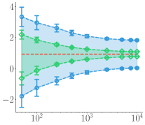
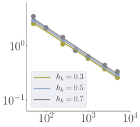
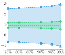
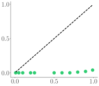
(a) Transitions, $n$	(b) Transitions, $n$	$(c)~{}1-\delta$	$(d)~{}\delta$

Figure 1: Results on Inverted-Pendulum. (a) The confidence interval (significance level $\delta=0.1$) of our method (green) and that of Feng et al. (2020) (blue) when varying the data size $n$. (b) The length of the confidence intervals ($\delta=0.1$) of our method scaling with the data size $n$. (c) The confidence intervals when we vary the significance level $\delta$ (data size $n=5000$). (d) The significance level $\delta$ vs. the empirical failure rate $\hat{\delta}$ of capturing the true expected reward by our confidence intervals (data size $n=5000$). We average over 50 random trials for each experiment.

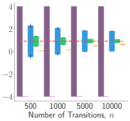
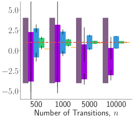
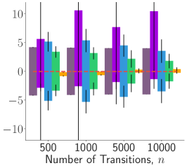
(a) Pendulum	(b) CartPole	(c) Type 1 diabetes

Figure 2: Results on different environments when we use a significance level of $\delta=0.1$. The colored bars represent the confidence intervals of different methods (averaged over 50 random trials); the black error bar represents the stand derivation of the end points of the intervals over the 50 random trials.

Results

Figure 1 shows our method obtains much tighter bounds than Feng et al. (2020), which is because we use a much tighter concentration inequality, even the dual bound that we use can be slightly looser than the primal bound used in Feng et al. (2020). Our method is also more computationally efficient than that of Feng et al. (2020) because the dual bound can be tightened approximately while the primal bound requires to solve a global optimization problem. Figure 1 (b) shows that we provide increasingly tight bounds as the data size $n$ increases, and the length of the interval decays with an $O(n^{-1/2})$ rate approximately. Figure 1 (c) shows that when we increase the significance level $\delta$, our bounds become tighter while still capturing the ground truth. Figure 1 (d) shows the percentage of times that the interval fails to capture the true value in a total of $100$ random trials (denoted as $\hat{\delta}$) as we vary $\delta$. We can see that $\hat{\delta}$ remains close to zero even when $\delta$ is large, suggesting that our bound is very conservative. Part of the reason is that the bound is constructed by considering the worse case and we used a conservative choice of the radius $r_{\mathcal{Q}}$ and coefficient $c_{q_{\pi},k}$ in Eq. (27) (See Appendix H.2).

In Figure 2 we compare different algorithms on more examples with $\delta=0.1$. We can again see that our method provides tight and conservative interval that always captures the true value. Although FQE (Bootstrap) yields tighter intervals than our method, it fail to capture the ground truth much more often than the promised $\delta=0.1$ (e.g., it fails in all the random trials in Figure 2 (a)).

We conduct more ablation studies on different hyper-parameter and data collecting procedure. See Appendix H.2 and H.3 for more details.

8 Conclusion and Future Directions

We develop a practical algorithm for constructing non-asymptotic confidence intervals for infinite-horizon off-policy evaluation with a very mild data assumption that holds for behavior-agnostic and time-dependent data. Our work opens a number of future direction: how to apply our bounds to develop new methods for safe policy optimization and safe exploration? how to develop rigorous and practical approaches to select $\mathcal{Q}$ and $\mathcal{W}$ adaptively based on the observed data, including their kernel, bandwidth and the radius of ball? how to extend our method to obtain bounds for different target policies $\pi$ (see e.g., Yin et al. (2020)) and initial distributions $\mathsf{D}_{0}$ simultaneously and computationally efficiently, without repeatedly solving the optimization in each case? The oracle bound in Eq. (28) provides a notion of oracle bound given the information drawn from the empirical Bellman operator. Is it possible to obtain even tighter bounds by exploiting other information from data, by e.g., model-based methods?

Appendix

Appendix A Proof of Lemma 4.2

Proof.

By assumption, we can write any ${}_{/}0\in\widetilde{\mathcal{W}}$ into ${}_{/}0(x)=\lambda(/x)$ where $\lambda\geq 0$ and $\in/\mathcal{W}$. Therefore, following Eq (18), we have

$$\inf_{\in/\widetilde{\mathcal{W}}}M(q,;/~{}\mathsf{D}_{\infty}) =\inf_{{}_{/}0\in\widetilde{\mathcal{W}}}\left\{\mathbb{E}_{\mathsf{D}_{\pi,0}}[q]-\mathbb{E}_{\mathsf{D}_{\infty}}[_{/}0(x)\hat{\mathbf{R}}q(x,y)]\right\}$$

$$=\inf_{\lambda\geq 0}\inf_{\in/\mathcal{W}}\left\{\mathbb{E}_{\mathsf{D}_{\pi,0}}[q]-\lambda\mathbb{E}_{\mathsf{D}_{\infty}}[(/x)\hat{\mathbf{R}}q(x,y)]\right\}$$

$$=\inf_{\lambda\geq 0}\left\{\mathbb{E}_{\mathsf{D}_{\pi,0}}[q]-\lambda L_{\mathcal{W}}(q,~{}\mathsf{D}_{\infty})\right\},$$

where we used the definition that $L_{\mathcal{W}}(q,~{}\mathsf{D}_{\infty})=\sup_{\in/\mathcal{W}}\mathbb{E}_{\mathsf{D}_{\infty}}[(/x)\hat{\mathbf{R}}q(x,y)]$.

For Eq (21), we note that

$$\mathbb{E}_{\mathsf{D}_{\pi,0}}[q(x)]-\mathbb{E}_{\mathsf{D}_{\infty}/[\hat{\mathbf{R}}q(x,y)]} =\mathbb{E}_{\mathsf{D}_{\pi,0}}[q(x)]-\mathbb{E}_{\mathsf{D}_{\infty}/[q(x)-\gamma q(x^{\prime})-r]}$$

$$=\mathbb{E}_{\mathsf{D}_{\infty}/[r]+\Delta(\mathsf{D}_{\infty}^{,}/~{}q),}$$

where we use the definition of $\Delta(\mathsf{D}_{\infty}^{,}/~{}q)$ in Eq (4.2). Therefore,

$$\sup_{q\in\mathcal{Q}}M(q,;/~{}\mathsf{D}_{\infty}) =\sup_{q\in\mathcal{Q}}\left\{\mathbb{E}_{\mathsf{D}_{\pi,0}}[q]-\mathbb{E}_{\mathsf{D}_{\infty}/[\hat{\mathbf{R}}q(x,y)]\right\}}$$

$$=\sup_{q\in\mathcal{Q}}\left\{\mathbb{E}_{\mathsf{D}_{\infty}/[r]+\Delta(\mathsf{D}_{\infty}^{,}/~{}q)\right\}}$$

$$=\mathbb{E}_{\mathsf{D}_{\infty}/[r]+I_{\mathcal{Q}}(;/~{}\mathsf{D}_{\infty}).}$$

∎

Appendix B Proof of the Dual Bound in Theorem 6.5

Proof.

Note that we assumed that $\mathcal{W}$ is the unit ball of the normed space $\widetilde{\mathcal{W}}$. Therefore, we can write any /in $\widetilde{\mathcal{W}}$ into $(/x)=\lambda h(x)$ with $\lambda\in\mathbb{R}$, $h\in\mathcal{W}$ and $\left\|\right/\|_{\widetilde{\mathcal{W}}}=\lambda$.

Using Lagrange multiplier, the bound in Eq. (31) is equivalent to

$${\hat{J}^{+}}_{\mathcal{Q},\mathcal{W}} =\sup_{q\in\mathcal{Q}}\inf_{\lambda\geq 0}\left\{\mathbb{E}_{\mathsf{D}_{\pi,0}}[q]~{}-~{}\lambda\left(\sup_{h\in\mathcal{W}}\frac{1}{n}\sum_{i=1}^{n}h(x_{i})\hat{\mathbf{R}}q(x_{i},y_{i})-\varepsilon_{n}\right)\right\}$$

$$=\sup_{q\in\mathcal{Q}}\inf_{\lambda\geq 0}\inf_{h\in\mathcal{W}}\left\{\mathbb{E}_{\mathsf{D}_{\pi,0}}[q]~{}-~{}\lambda\left(\frac{1}{n}\sum_{i=1}^{n}h(x_{i})\hat{\mathbf{R}}q(x_{i},y_{i})-\varepsilon_{n}\right)\right\}$$

$$=\sup_{q\in\mathcal{Q}}\inf_{\in/\widetilde{\mathcal{W}}}\left\{\mathbb{E}_{\mathsf{D}_{\pi,0}}[q]~{}-~{}\frac{1}{n}\sum_{i=1}^{n}(/x_{i})\hat{\mathbf{R}}q(x_{i},y_{i})+\varepsilon_{n}\left\|\right/\|_{\widetilde{\mathcal{W}}}\right\}\,,$$

Define

$$\hat{M}(q,~{};/~{}\hat{\mathsf{D}}_{n}) =\mathbb{E}_{\mathsf{D}_{\pi,0}}[q]~{}-\frac{1}{n}\sum_{i=1}^{n}(/x_{i})\hat{\mathbf{R}}q(x_{i},y_{i})+\varepsilon_{n}\left\|\right/\|_{\widetilde{\mathcal{W}}}$$

$$=\mathbb{E}_{\hat{\mathsf{D}}_{n}/[r]+\Delta(\hat{\mathsf{D}}_{n}^{,}/~{}q)+\varepsilon_{n}\left\|\right/\|_{\widetilde{\mathcal{W}}}.}$$

Then we have

$$\sup_{q\in\mathcal{Q}}\hat{M}(q,~{};/~{}\hat{\mathsf{D}}_{n}) =\mathbb{E}_{\hat{\mathsf{D}}_{n}/[r]+\sup_{q\in\mathcal{Q}}\Delta(\hat{\mathsf{D}}_{n}^{,}/~{}q)+\varepsilon_{n}\left\|\right/\|_{\widetilde{\mathcal{W}}}}$$

$$=\mathbb{E}_{\hat{\mathsf{D}}_{n}/[r]+I_{\mathcal{Q}}(\omega;~{}\hat{\mathsf{D}}_{n})+\varepsilon_{n}\left\|\right/\|_{\widetilde{\mathcal{W}}}}$$

$$:=\hat{F}^{+}_{\mathcal{Q}}()/.$$

Therefore,

$${\hat{J}^{+}}_{\mathcal{Q},\mathcal{W}} =\sup_{q\in\mathcal{Q}}\inf_{\in/\widetilde{\mathcal{W}}}M(q,~{};/~{}\hat{\mathsf{D}}_{n})$$

$$\leq\inf_{\in/\widetilde{\mathcal{W}}}\sup_{q\in\mathcal{Q}}M(q,~{};/~{}\hat{\mathsf{D}}_{n})$$

$$=\inf_{\in/\widetilde{\mathcal{W}}}\hat{F}^{+}_{\mathcal{Q}}()/.$$

The lower bound follows analogously. The strong duality holds when the Slater's condition (Nesterov, 2003) is satisfied, which amounts to saying that the primal problem in Eq. (31) is convex and strictly feasible; this requires that $\mathcal{Q}$ is convex and there exists at least one solution $q\in\mathcal{Q}$ that satisfies that constraint strictly, that is, $L_{\mathcal{W}}(q;~{}\hat{\mathsf{D}}_{n})<\varepsilon_{n}$; note that in our case the objective function $\mathcal{Q}$ is linear on $q$ and the constraint function $L_{\mathcal{W}}(q;~{}\hat{\mathsf{D}}_{n})$ is always convex on $q$ (since it is the sup a set of linear functions on $q$ following Eq. (8)).

∎

Appendix C Proof of Concentration Bound in Theorem 5.1

Our proof requires the following Hoeffding inequality on Hilbert spaces by Pinelis (Theorem 3, 1992); see also Section 2.4 of Rosasco et al. (2010).

Lemma C.1.

(Theorem 3, Pinelis, 1992) Let $\mathcal{H}$ be a Hilbert space and $\{f_{i}\}_{i=1}^{n}$ is a martingale difference sequence in $\mathcal{H}$ that satisfies $\sup_{i}\left\|f_{i}\right\|_{\mathcal{H}}\leq\sigma$ almost surely. We have for any $\epsilon>0$,

$$\mathrm{Pr}\left(\left\|\frac{1}{n}\sum_{i=1}^{n}f_{i}\right\|_{\mathcal{H}}\geq\epsilon\right)\leq 2\exp\left(-\frac{n\epsilon^{2}}{2\sigma^{2}}\right).$$

Therefore, for $\delta\in(0,1)$, with probability at least $1-\delta$, we have $\left\|\frac{1}{n}\sum_{i=1}^{n}f_{i}\right\|_{\mathcal{H}}\leq\sqrt{\frac{2\sigma^{2}\log(2/\delta)}{n}}.$

Lemma C.2.

Let $k(x,x^{\prime})$ be a positive definite kernel whose RKHS is $\mathcal{H}_{k}$. Define

$$f_{i}(\cdot)=\hat{{\mathbf{R}}}q(x_{i},y_{i})k(x_{i},\cdot)-{\mathbf{R}}q(x_{i})k(x_{i},\cdot).$$

Assume Assumption 2.1 holds, then $\{f_{i}\}_{i=1}^{n}$ is a martingale difference sequence in $\mathcal{H}_{k}$ w.r.t. $T_{<i}:=(x_{j},y_{j})_{j<i}\cup(x_{i})$. That is, $\mathbb{E}\left[f_{i+1}(\cdot)~{}|~{}T_{<i}\right]=0$ for $i=1,\ldots,n$. In addition,

$$\left\|\frac{1}{n}\sum_{i=1}^{n}f_{i}\right\|^{2}_{\mathcal{H}_{k}}=\frac{1}{n^{2}}\sum_{ij=1}^{n}\left(\hat{{\mathbf{R}}}q(x_{i},y_{i})-{\mathbf{R}}q(x_{i})\right)k(x_{i},x_{j})\left(\hat{{\mathbf{R}}}q(x_{j},y_{j})-{\mathbf{R}}q(x_{j})\right),$$

and $\left\|f_{i}\right\|_{\mathcal{H}_{k}}^{2}\leq c_{q,k}$ for $\forall i=1,\ldots,n$.

Proof of Theorem 5.1.

Following Lemma C.1 and Lemma C.2, since $\{f_{i}\}_{i=1}^{n}$ is a martingale difference sequence in $\mathcal{H}_{k}$ with $\left\|f_{i}\right\|_{\mathcal{H}_{k}}^{2}\leq c_{q,k}$ almost surely, we have with probability at least $1-\delta$,

$$\frac{1}{n^{2}}\sum_{ij=1}^{n}\left(\hat{{\mathbf{R}}}q(x_{i},y_{i})-{\mathbf{R}}q(x_{i})\right)k(x_{i},x_{j})\left(\hat{{\mathbf{R}}}q(x_{j},y_{j})-{\mathbf{R}}q(x_{j})\right)=\left\|\frac{1}{n}\sum_{i=1}^{n}f_{i}\right\|_{\mathcal{H}_{k}}^{2}\leq\frac{2c_{q,k}\log(2/\delta)}{n}.$$

Using Lemma C.3 below, we have

$$\left|{L_{\mathcal{K}}(q;~{}\hat{\mathsf{D}}_{n})}-{L^{*}_{\mathcal{K}}(q;~{}\hat{\mathsf{D}}_{n})}\right|\leq\left\|\frac{1}{n}\sum_{i=1}^{n}f_{i}\right\|_{\mathcal{H}_{k}}\leq\sqrt{\frac{2c_{q,k}\log(2/\delta)}{n}}.$$

This completes the proof. ∎

Lemma C.3.

Assume $k(x,x^{\prime})$ is a positive definite kernel. We have

$$\left|{L_{\mathcal{K}}(q;~{}\hat{\mathsf{D}}_{n})}-{L^{*}_{\mathcal{K}}(q;~{}\hat{\mathsf{D}}_{n})}\right|^{2}\leq\frac{1}{n^{2}}\sum_{ij=1}^{n}\left(\hat{{\mathbf{R}}}q(x_{i},y_{i})-{\mathbf{R}}q(x_{i})\right)k(x_{i},x_{j})\left(\hat{{\mathbf{R}}}q(x_{j},y_{j})-{\mathbf{R}}q(x_{j})\right).$$

Proof.

Define

$$\hat{g}(\cdot)=\frac{1}{n}\sum_{i=1}^{n}\hat{{\mathbf{R}}}q(x_{i},y_{i})k(x_{i},\cdot), g(\cdot)=\frac{1}{n}\sum_{i=1}^{n}{\mathbf{R}}q(x_{i})k(x_{i},\cdot).$$

Then we have

$$\left\|\hat{g}\right\|_{\mathcal{H}_{k}}^{2}=\frac{1}{n^{2}}\sum_{ij=1}^{n}\hat{{\mathbf{R}}}q(x_{i},y_{i})k(x_{i},x_{j})\hat{{\mathbf{R}}}q(x_{j},y_{j})=\hat{L}_{\mathcal{K}}(q;~{}\hat{\mathsf{D}}_{n})^{2},$$

$$\left\|g\right\|_{\mathcal{H}_{k}}^{2}=\frac{1}{n^{2}}\sum_{ij=1}^{n}{\mathbf{R}}q(x_{i})k(x_{i},x_{j}){\mathbf{R}}q(x_{j})=L^{*}_{\mathcal{K}}(q;~{}\hat{\mathsf{D}}_{n})^{2},$$

$$\left\|\hat{g}-g\right\|_{\mathcal{H}_{k}}^{2}=\frac{1}{n^{2}}\sum_{ij=1}^{n}\left(\hat{{\mathbf{R}}}q(x_{i},y_{i})-{\mathbf{R}}q(x_{i})\right)k(x_{i},x_{j})\left(\hat{{\mathbf{R}}}q(x_{j},y_{j})-{\mathbf{R}}q(x_{j})\right).$$

The result then follows the triangle inequality $\left|\left\|\hat{g}\right\|_{\mathcal{H}_{k}}-\left\|g\right\|_{\mathcal{H}_{k}}\right|\leq\left\|\hat{g}-g\right\|_{\mathcal{H}_{k}}.$ ∎

C.1 Calculation of $c_{q_{*},k}$

The practical calculation of the coefficient $c_{q_{*},k}$ in the concentration inequality was discussed in Feng et al. (2020), which we include here for completeness.

Lemma C.4.

(Feng et al. (2020) Lemma 3.1) Assume the reward function and kernel function is bounded with $\sup_{x}|r(x)|\leq r_{\max}$ and $\sup_{x,x^{\prime}}|k(x,x^{\prime})|\leq K_{\max}$, we have:

$$c_{q_{*},k}:=\sup_{x\in\mathcal{X},y\in\mathcal{Y}}({\hat{\mathbf{R}}}q_{*}(x,y))^{2}k(x,x)\leq\frac{4K_{\max}r^{2}_{\max}}{(1-\gamma)^{2}}\,.$$ (38)

In practice, we evaluate $K_{\max}$ from the kernel function that we choose (e.g., $K_{\max}=1$ for RBF kernels), and $r_{\max}$ from the knowledge of the environment.

Appendix D More Discussion on the Tightness of the Confidence Interval

The benefit of having both upper and lower bounds is that we can empirically access the tightness of the bound by checking the length of the interval $[\hat{F}^{-}_{\mathcal{Q}}(_{/}-),\hat{F}^{+}_{\mathcal{Q}}(_{/}+)]$. However, from the theoretical perspective, it is desirable to know a priori that the length of the interval will decrease with a fast rate as the data size $n$ increases. We now show that this is the case if $\widetilde{\mathcal{W}}$ is chosen to be sufficiently rich so that it includes a $\in/\widetilde{\mathcal{W}}$ such that $\hat{\mathsf{D}}_{n}$/approximates $\mathsf{D}_{*}$ closely in a proper sense.

Theorem D.1.

Assume $\widetilde{\mathcal{W}}$ is sufficiently rich to include a ``good'' ${}_{*}/$ in $\widetilde{\mathcal{W}}$ with $\hat{\mathsf{D}}_{n}^{{}_{*}/}\approx\mathsf{D}_{*}$ in the sense that

$$\sup_{q\in\mathcal{Q}}\left|\mathbb{E}_{\hat{\mathsf{D}}_{n}^{{}_{*}/}}\left[{\hat{\mathbf{R}}}q(x,y)\right]-\mathbb{E}_{\mathsf{D}_{*}}\left[{\hat{\mathbf{R}}}q(x,y)\right]\right|\leq\frac{c}{n^{\alpha}},$$ (39)

where $c$ and $\alpha$ are two positive coefficients. Then we have

$$\max\left\{{\hat{J}^{+}}_{\mathcal{Q},\mathcal{W}}-J_{*},~{}~{}J_{*}-{\hat{J}^{-}}_{\mathcal{Q},\mathcal{W}}\right\}\leq\frac{c}{n^{\alpha}}+\varepsilon_{n}\left\|{}_{*}/\right\|_{\widetilde{\mathcal{W}}}.$$

Assumption (39) holds if $\hat{\mathsf{D}}_{n}$ is collected following a Markov chain that has certain strong mixing condition and weakly converges to a limit continuous discussion $\mathsf{D}_{\infty}$ whose support is $\mathcal{X}$, and the density ratio between $\mathsf{D}_{*}$ and $\mathsf{D}_{\infty}$, denoted by ${}_{*}/$, is included in $\widetilde{\mathcal{W}}$. In this case, if $\mathcal{Q}$ is a finite ball in RKHS, then we can achieve Eq. (39) with $\alpha=1/2$, and yields the overall bound of rate $O(n^{-1/2})$. For more general function classes, $\alpha$ depends on the martingale Rademacher complexity of the function set $\hat{\mathbf{R}}\mathcal{Q}=\{{\mathbf{R}}q(x,y)\colon q\in\mathcal{Q}\}$ (Rakhlin et al., 2015). In our empirical reults, we observe that the lengths of the practically constructed confidence intervals do tend to follow the $O(n^{-1/2})$ rate approximately; see Figure 1(b)

Proof.

Note that $\gamma q(x^{\prime})-q(x)=-\hat{\mathbf{R}}q(x,y)-r$ and hene

$$I_{\mathcal{Q}}(\omega;~{}\hat{\mathsf{D}}_{n}) =\sup_{q\in\mathcal{Q}}\left\{\mathbb{E}_{\hat{\mathsf{D}}_{n}/[\gamma q(x^{\prime})-q(x)]-\mathbb{E}_{\mathsf{D}_{*}}[\gamma q(x^{\prime})-q(x)]\right\}}$$

$$=\sup_{q\in\mathcal{Q}}\left\{\mathbb{E}_{\mathsf{D}_{*}}[\hat{\mathbf{R}}q(x,y)]-\mathbb{E}_{\hat{\mathsf{D}}_{n}/[\hat{\mathbf{R}}q(x,y)]\right\}+\mathbb{E}_{\mathsf{D}_{*}}[r]-\mathbb{E}_{\hat{\mathsf{D}}_{n}/[r].}}$$

Because ${}_{*}/\in\mathcal{W}$, we have

$${\hat{J}^{+}}_{\mathcal{W},\mathcal{Q}}-J_{*} \leq\hat{F}^{+}_{\mathcal{Q}}(_{*}/)-J_{*}$$

$$=\mathbb{E}_{\hat{\mathsf{D}}_{n}/[r]+I_{\mathcal{Q}}(\omega_{\pi};~{}\hat{\mathsf{D}}_{n})+\varepsilon_{n}\left\|{}_{*}/\right\|_{\widetilde{\mathcal{W}}}-\mathbb{E}_{\mathsf{D}_{*}}[r]}$$

$$=\sup_{q\in\mathcal{Q}}\left\{\mathbb{E}_{\mathsf{D}_{*}}\left[{\hat{\mathbf{R}}}q(x,y)\right]-\mathbb{E}_{\hat{\mathsf{D}}_{n}/\left[{\hat{\mathbf{R}}}q(x,y)\right]\right\}+\varepsilon_{n}\left\|{}_{*}/\right\|_{\widetilde{\mathcal{W}}}}$$

$$\leq\frac{c}{n^{\alpha}}+\varepsilon_{n}\left\|{}_{*}/\right\|_{\widetilde{\mathcal{W}}}.$$

The case of lower bound follows similarly. ∎

Appendix E Practical Optimization on $\widetilde{\mathcal{W}}$

Consider the optimization of /in $\widetilde{\mathcal{W}}$,

$$\hat{F}^{+}_{\mathcal{Q}}(\omega):=\frac{1}{n}\sum_{i=1}^{n}{r_{i}(/x_{i})}+I_{\mathcal{Q}}(\omega;~{}\hat{\mathsf{D}}_{n})+\left\|\right/\|_{\widetilde{\mathcal{W}}}\sqrt{\frac{{2}c_{q_{*},k}\log(2/\delta)}{n}}.$$ (40)

Assume $\widetilde{\mathcal{W}}$ is the RKHS of kernel $k(x,\bar{x})$. By the finite representer theorem of RKHS (Scholkopf and Smola, 2018), the optimization of $\omega\in\widetilde{\mathcal{W}}$ can be reduced to a finite dimensional optimization problem. Specifically, the optimal solution of (40) can be written into a form of $(/x)=\sum_{i=1}^{n}k(x,x_{i})\alpha_{i}$ for which we have $\left\|\right/\|_{\mathcal{H}_{k}}^{2}=\sum_{i,j=1}^{n}k(x_{i},x_{j})\alpha_{i}\alpha_{j}$ for some vector $\bm{\alpha}:=[\alpha_{i}]_{i=1}^{n}\in\mathbb{R}^{n}$. Write $\bm{K}=[k(x_{i},x_{j})]_{i,j=1}^{n}$ and $\bm{r}=[r_{i}]_{i=1}^{n}$. The optimization of /reduces to solving the following optimization on $\bm{\alpha}$:

$$\min_{\bm{\alpha}\in\mathbb{R}^{n}}\left\{\frac{1}{n}\bm{r}^{\top}\bm{K}\bm{\alpha}+I_{\mathcal{Q}}(\bm{K}\bm{\alpha};~{}\hat{\mathsf{D}}_{n})+\sqrt{\bm{\alpha}\bm{K}\bm{\alpha}}\sqrt{\frac{{2}c_{q_{*},k}\log(2/\delta)}{n}}\right\}\,,$$

where

$$I_{\mathcal{Q}}(\bm{K}\bm{\alpha};~{}\hat{\mathsf{D}}_{n})=\max_{q\in\mathcal{Q}}\left\{\mathbb{E}_{\mathsf{D}_{\pi,0}}[q]+\frac{1}{n}(\hat{{\mathbf{T}}}q)^{\top}\bm{K}\bm{\alpha}\right\},$$

and $\hat{{\mathbf{T}}}q=[\gamma q(x^{\prime}_{i})-q(x_{i})]_{i=1}^{n}\in\mathbb{R}^{n}$. When $\mathcal{Q}$ is a finite ball of an RKHS (that is different from $\widetilde{\mathcal{W}}$), we can calculate $I_{\mathcal{Q}}(\bm{K}\bm{\alpha};~{}\hat{\mathsf{D}}_{n})$ using Eq. (15).

This computation can be still expensive when $n$ is large. Fortunately, our confidence bound holds correctly for any /; better /only gives tighter bounds, but it is not necessary to find the exact global optimal /. Therefore, one can use any approximation algorithm to find /, which provides a trade-off of tightness and computational cost. We discuss two methods:

1) Approximating $\bm{\alpha}$

The length of $\bm{\alpha}$ can be too large when $n$ is large. To address this, we assume $\alpha_{i}=g(x_{i},~{}\theta)$, where $g$ is any parametric function (such as a neural network) with a parameter $\theta$; assume $\theta$ has a much lower dimension than $\bm{\alpha}$. We can then optimize $\theta$ with stochastic gradient descent, by approximating the empirical averaging $\frac{1}{n}\sum_{i=1}^{n}(\cdot)$ in the objective with averages over small mini-batches; this would introduce biases in gradient estimation, but it is not an issue when the goal is only to get a reasonable approximation of the optimal /.

2) Replacing kernel $\bm{k}$

Assume the kernel $k(x,\bar{x})$ yields a random feature expansion of form $k(x,\bar{x})=\mathbb{E}_{\beta\sim\pi}[\phi(x,\beta)\phi(\bar{x},\beta)]$, where $\phi(x,\beta)$ is a feature map with parameter $\beta$ and $\pi$ is a distribution of $\beta$. We draw $\{\beta_{i}\}_{i=1}^{m}$ i.i.d. from $\pi$, where $m$ is taken to be much smaller than $n$. We replace $k$ with $\hat{k}(x,\bar{x})=\frac{1}{m}\sum_{i=1}^{m}\phi(x,\beta_{i})\phi(\bar{x},\beta_{i})$ and let $\widehat{\mathcal{W}}$ to be the RKHS of kernel $\hat{k}$. Then, we consider to solve

$${\hat{J}^{+}}_{\mathcal{Q},\mathcal{W}}=\min_{\in/\widehat{\mathcal{W}}}\left\{\hat{F}^{+}_{\mathcal{Q}}(\omega):=\frac{1}{n}\sum_{i=1}^{n}{r_{i}(/x_{i})}+I_{\mathcal{Q}}(\omega;~{}\hat{\mathsf{D}}_{n})+\left\|\right/\|_{\widehat{\mathcal{W}}}\sqrt{\frac{{2}c_{q_{*},\hat{k}}\log(2/\delta)}{n}}\right\}.$$

It is known that any function /in $\widehat{\mathcal{W}}$ can be represented as $(/x)=\frac{1}{m}\sum_{i=1}^{m}w_{i}\phi(x,\beta_{i}),$ for some $\bm{w}=[w_{i}]_{i=1}^{m}\in\mathbb{R}^{m}$ and satisfies $\left\|\right/\|_{\widehat{\mathcal{W}}}^{2}=\frac{1}{m}\sum_{i=1}^{m}w_{i}^{2}.$ In this way, the problem reduces to optimizing an $m$-dimensional vector $\bm{w}$, which can be (approximately) solved by standard convex optimization techniques.

Appendix F Concentration Inequality of General Functional Bellman Losses

Theorem 5.1 provides the concentration inequality of $L_{\mathcal{W}}(q;~{}\hat{\mathsf{D}}_{n})$ when $\mathcal{W}$ is the unit ball of an RKHS. When $\mathcal{W}$ is a general function set, one can still obtain a general concentration bound using Radermacher complexity. Define $\hat{\mathbf{R}}q\circ\mathcal{W}:=\{h(x,y)=\hat{\mathbf{R}}q(x,y)(/x)\colon\in/\mathcal{W}\}$. Using the standard derivation in Radermacher complexity theory in conjunction with Martingale theory (Rakhlin et al., 2015), we have

$$\sup_{\in/\mathcal{W}}\left\{\frac{1}{n}\sum_{i=1}^{n}(\hat{\mathbf{R}}q(x_{i},y_{i})-{\mathbf{R}}q(x_{i}))(/x_{i})\right\}\leq 2Rad(\hat{\mathbf{R}}q\circ\mathcal{W})+\sqrt{\frac{2c_{q,\mathcal{W}}\log(2/\delta)}{n}},$$

where $c_{q,\mathcal{W}}=\sup_{\in/\mathcal{W}}\sup_{x,y}(\hat{\mathbf{R}}q(x,y)-{\mathbf{R}}q(x))^{2}(/x)^{2}$ and $Rad(\hat{\mathbf{R}}q\circ\mathcal{W})$ is the sequential Radermacher complexity (Rakhlin et al., 2015). A triangle inequality yields

$$|~{}L_{\mathcal{W}}(q;~{}\hat{\mathsf{D}}_{n})-L^{*}_{\mathcal{W}}(q;~{}\hat{\mathsf{D}}_{n})~{}|\leq\sup_{\in/\mathcal{W}}\left\{\frac{1}{n}\sum_{i=1}^{n}(\hat{\mathbf{R}}q(x_{i},y_{i})-{\mathbf{R}}q(x_{i}))(/x_{i})\right\}.$$

Therefore,

$$|~{}L_{\mathcal{W}}(q;~{}\hat{\mathsf{D}}_{n})-L^{*}_{\mathcal{W}}(q;~{}\hat{\mathsf{D}}_{n})~{}|\leq 2Rad(\hat{\mathbf{R}}q\circ\mathcal{W})+\sqrt{\frac{2c_{q,\mathcal{W}}\log(2/\delta)}{n}}.$$ (41)

When $\mathcal{W}$ equals the unit ball $\mathcal{K}$ of the RKHS of kernel $k$, we have $c_{q,k}=c_{q,\mathcal{W}}$ and hence this bound is strictly worse than the bound in Theorem 5.1.

Appendix G More on the Oracle Bound and its Dual Form

The oracle bound (28) provides another starting point for deriving optimization-based confidence bounds. We start with deriving the dual form of (28). Using Lagrangian multiplier, the optimization in Eq. (28) can be rewritten into

$$\hat{J}_{\mathcal{Q},*}^{+}=\sup_{q\in\mathcal{Q}}\inf/M_{*}(q,;/~{}\hat{\mathsf{D}}_{n})\leq\inf/\sup_{q\in\mathcal{Q}}M_{*}(q,;/~{}\hat{\mathsf{D}}_{n}),$$ (42)

where

$$M_{*}(q,;/~{}\hat{\mathsf{D}}_{n})=\mathbb{E}_{\mathsf{D}_{\pi,0}}[q]-\frac{1}{n}\sum_{i=1}^{n}(/x_{i})\left(\hat{\mathbf{R}}q(x_{i},y_{i})-\hat{\mathbf{R}}q_{*}(x_{i},y_{i})\right),$$

and /is optimized in the set of all functions and serves as the Lagrangian multiplier here. Define

$$\hat{F}_{\mathcal{Q},*}^{+}()/ :=\max_{q\in\mathcal{Q}}M_{*}(q,;/~{}\hat{\mathsf{D}}_{n})$$

$$=\underbrace{\mathbb{E}_{\hat{\mathsf{D}}_{n}/[r]+I_{\mathcal{Q}}(\omega;~{}\hat{\mathsf{D}}_{n})}_{known}+\underbrace{R(,/~{}q_{*})}_{unknown}}$$

where

$$R(,/q_{*})=\frac{1}{n}\sum_{i=1}^{n}(/x_{i})\hat{\mathbf{R}}q_{*}(x_{i}).$$

Then by the weak duality, we have

$$J_{\mathcal{Q},+}^{*}\leq\hat{F}_{\mathcal{Q},*}^{+}()/,~{}~{}~{}~{}\forall./$$

The derivation follows similarly for the lower bound. So for any $\in/\widetilde{\mathcal{W}}$, we have $[\hat{J}_{\mathcal{Q},*}^{-},~{}~{}\hat{J}_{\mathcal{Q},*}^{+}]\subseteq[\hat{F}_{\mathcal{Q},*}^{-}()/,~{}~{}\hat{F}_{\mathcal{Q},*}^{+}()/].$

Here the first two terms of $\hat{F}_{\mathcal{Q},*}^{+}()/$ can be empirically estimated (it is the same as the first two terms of Eq. (36)), but the third term $R(,/q_{*})$ depends on the unknown $q_{*}$ and hence need to be further upper bounded. Different upper bounds of $R(,/q_{*})$ may yield different practical confidence intervals.

Our method can be viewed as constraining /in the unit ball $\mathcal{W}$ of a normed function space $\widetilde{\mathcal{W}}$, and applying a worst case bound: for any $\in/\widetilde{\mathcal{W}}$, we have

$$\hat{F}_{\mathcal{Q},*}^{+}()/ :=\mathbb{E}_{\hat{\mathsf{D}}_{n}/[r]+I_{\mathcal{Q}}(\omega;~{}\hat{\mathsf{D}}_{n})+R(,/~{}q_{*})}$$

$$\leq\mathbb{E}_{\hat{\mathsf{D}}_{n}/[r]+I_{\mathcal{Q}}(\omega;~{}\hat{\mathsf{D}}_{n})+\left\|w\right\|_{\widetilde{\mathcal{W}}}\sup_{h\in\mathcal{W}}R(h,~{}q_{*})}$$

$$\leq\mathbb{E}_{\hat{\mathsf{D}}_{n}/[r]+I_{\mathcal{Q}}(\omega;~{}\hat{\mathsf{D}}_{n})+\left\|w\right\|_{\widetilde{\mathcal{W}}}L_{\mathcal{W}}(q_{*},\hat{\mathsf{D}}_{n})}$$

$$\overset{w.p.1-\delta}{\leq}\mathbb{E}_{\hat{\mathsf{D}}_{n}/[r]+I_{\mathcal{Q}}(\omega;~{}\hat{\mathsf{D}}_{n})+\varepsilon_{n}\left\|w\right\|_{\widetilde{\mathcal{W}}}}$$

$$=\hat{F}_{\mathcal{Q}}^{+}()/,$$

where we note that $L_{\mathcal{W}}(q_{*},\hat{\mathsf{D}}_{n})=\sup_{h\in\mathcal{W}}R(h,~{}q_{*})$ and the last step applies the high probability bound that $\mathrm{Pr}(L_{\mathcal{W}}(q_{*},\hat{\mathsf{D}}_{n})\leq\varepsilon)\geq 1-\delta$. With the same derivation on the lower bound counterpart, we have

$$\mathrm{Pr}\left(\left[\hat{F}_{\mathcal{Q},*}^{-}()/,~{}~{}\hat{F}_{\mathcal{Q},*}^{+}()/\right]\subseteq\left[\hat{F}_{\mathcal{Q}}^{-}()/,\hat{F}_{\mathcal{Q}}^{+}()/\right]\right)\geq 1-\delta.$$

Therefore, our confidence bound $[\hat{F}_{\mathcal{Q}}^{-}()/,\hat{F}_{\mathcal{Q}}^{+}()/]$ is a $1-\delta$ confidence outer bound the oracle bound $[\hat{J}_{\mathcal{Q},*}^{-}()/,~{}~{}\hat{J}_{\mathcal{Q},*}^{+}()/]\subseteq[\hat{F}_{\mathcal{Q},*}^{-}()/,~{}~{}\hat{F}_{\mathcal{Q},*}^{+}()/]$.

G.1 Proof of Proposition  6.2

Proof.

Let $\mathcal{Q}_{\mathrm{null}}$ be the set of functions that are zero on $\{s_{i},s_{i}^{\prime}\}_{i=1}^{n}$, that is,

$$\mathcal{Q}_{\mathrm{null}}=\{g\colon\mathcal{S}\times\mathcal{A}\to\mathbb{R}\colon~{}~{}g(s,a)=0,~{}~{}\forall s\in\{s_{i},s_{i}^{\prime}\}_{i=1}^{n},~{}~{}~{}a\in\mathcal{A}\}.$$

Then we have

$$\hat{\mathbf{R}}(q_{*}+g)(x_{i},y_{i})=\hat{\mathbf{R}}q_{*}(x_{i},y_{i}),~{}~{}~{}~{}~{}\forall i=1,\ldots,n.$$

and

$$\mathbb{E}_{\mathsf{D}_{\pi,0}}[q_{*}+g]=\mathbb{E}_{\mathsf{D}_{*},0}[q_{*}]+\mathbb{E}_{\mathsf{D}_{\pi,0}}[g]=J_{*}+\mathbb{E}_{\mathsf{D}_{\pi,0}}[g].$$

Taking $g(s,a)=z\mathbb{I}(s\notin\{s_{i},s_{i}^{\prime}\}_{i=1}^{n})$, where $z$ is any real number. Then we have

$$\mathbb{E}_{\mathsf{D}_{\pi,0}}[q_{*}+g]=J_{*}+z\mathrm{Pr}_{s\sim\mathsf{D}_{\pi,0}}(s\notin\{s_{i},s_{i}^{\prime}\}_{i=1}^{n}).$$

Because $\mathrm{Pr}_{s\sim\mathsf{D}_{\pi,0}}(s\notin\{s_{i},s_{i}^{\prime}\}_{i=1}^{n})\neq 0$, we can take $z$ to be arbitrary value to make $\mathbb{E}_{\mathsf{D}_{\pi,0}}[q_{*}+g]$ to take arbitrary value. ∎

Appendix H Ablation Study and Experimental Details

H.1 Experimental Details

Environments and Dataset Construction

We test our method on three environments: Inverted-Pendulum and CartPole from OpenAI Gym (Brockman et al., 2016), and a Type-1 Diabetes medical treatment simulator. For Inverted-Pendulum we discretize the action space to be $\{-1,-0.3,-0.2,0,0.2,0.3,1\}$. The action space of CartPole and the medical treatment simulator are both discrete.

Policy Construction

We follow a similar setup as Feng et al. (2020) to construct behavior and target policies. For all of the environments, we constraint our policy class to be a softmax policy and use PPO (Schulman et al., 2017) to train a good policy $\pi$, and we use different temperatures of the softmax policy to construct the target and behavior policies (we set the temperature $\tau=0.1$ for target policy and $\tau=1$ to get the behavior policy, and in this way the target policy is more deterministic than the behavior policy). We consider other choices of behavior policies in Section H.3.

For horizon lengths, We fix $\gamma=0.95$ and set horizon length $H=50$ for Inverted-Pendulum, $H=100$ for CartPole, and $H=50$ for Diabetes simulator.

Algorithm Settings

We test the bound in Eq.(36)-(37). Throughout the experiment, we always set $\mathcal{W}=\mathcal{K}$, a unit ball of RKHS with kernel $k(\cdot,\cdot)$. We set $\mathcal{Q}=r_{\mathcal{Q}}\tilde{\mathcal{K}}$, the zero-centered ball of radius $r_{\mathcal{Q}}$ in an RKHS with kernel $\tilde{k}(\cdot,\cdot).$ We take both $k$ and $\tilde{k}$ to be Gaussian RBF kernel. The bandwidth of $k$ and $\tilde{k}$ are selected to make sure the function Bellman loss is not large on a validation set. The radius is selected to be sufficiently large to ensure that $q_{*}$ is included in $\mathcal{Q}$. To ensure a sufficiently large radius, we use the data to approximate a $\hat{q}$ so that its functional Bellman loss is small than $\epsilon_{n}$. Then we set $r_{\mathcal{Q}}=10*\|\hat{q}\|_{\tilde{\mathcal{K}}}$. We optimize /using the random feature approximation method described in Appendix E. Once ${}_{/}+$ and ${}_{/}-$ are found, we evaluate the bound in Eq. (36) exactly, to ensure the theoretical guarantee holds.

H.2 Sensitivity to Hyper-Parameters

We investigate the sensitivity of our algorithm to the choice of hyper-parameters. The hyper-parameter mainly depends on how we choose our function class $\mathcal{Q}$ and $\mathcal{W}$.

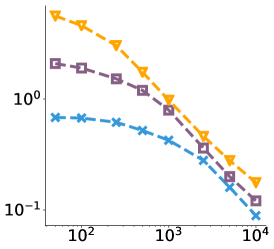
$\log_{10}(\text{interval length})$	Reward
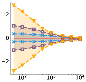
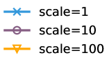
(a) Number of transitions, $n$	(b) Number of transitions  $n$

Figure 3: Ablation study on the radius $r_{\mathcal{Q}}$ of the function class $\mathcal{Q}$. The default collecting procedure uses a horizon length of $H=50$. The discounted factor is $\gamma=0.95$ by default.

Radius of $\mathcal{Q}$

Recall that we choose $\mathcal{Q}$ to be a ball in RKHS with radius $r_{\mathcal{Q}}$, that is,

$$\mathcal{Q}=r_{\mathcal{Q}}\tilde{\mathcal{K}}=\{r_{\mathcal{Q}}f:f\in\tilde{\mathcal{K}}\},$$

where $\tilde{\mathcal{K}}$ is the unit ball of the RKHS with kernel $\tilde{k}$. Ideally, we want to ensure that $r_{\mathcal{Q}}\geq\|q_{*}\|_{\tilde{\mathcal{K}}}$ so that $q_{*}\in\mathcal{Q}$.

Since it is hard to analyze the behavior of the algorithm when $q_{*}$ is unknown, we consider a synthetic environment where the true $q_{*}$ is known. This is done by explicitly specifying a $q_{*}$ inside $\tilde{\mathcal{K}}$ and then infer the corresponding deterministic reward function $r(x)$ by inverting the Bellman equation:

$$r(x):=q_{*}(x)-\gamma\mathbb{E}_{x^{\prime}\sim\mathsf{P}_{\pi}(\cdot|x)}[q_{*}(x^{\prime})].$$

Here $r$ is a deterministic function, instead of a random variable, with an abuse of notation. In this way, we can get access to the true RKHS norm of $q_{*}$:

$$\rho^{*}=\|q_{*}\|_{\tilde{\mathcal{K}}}\,.$$

For simplicity, we set both the state space $\mathcal{S}$ and action space $\mathcal{A}$ to be $\mathbb{R}$ and set a Gaussian policy $\pi(a|s)\propto\exp(f(s,a)/\tau)$, where $\tau$ is a positive temperature parameter. We set $\tau=0.1$ as target policy and $\tau=1$ as behavior policy.

Figure 3 shows the results as we set $r_{\mathcal{Q}}$ to be $\rho^{*}$, $10\rho^{*}$ and $100\rho^{*}$, respectively. We can see that the tightness of the bound is affected significantly by the radius when the number $n$ of samples is very small. However, as the number $n$ of samples grow (e.g., $n\geq 2\times 10^{3}$ in our experiment), the length of the bounds become less sensitive to the changing of the predefined norm of $\mathcal{Q}$.

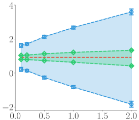
Reward	Interval length
Temperature $\tau$	Bandwidth of $k$ of $\widetilde{\mathcal{W}}$
(a) Varying temperature $\tau$.	(b) Varying the bandwidth of kernels in $\widetilde{\mathcal{W}}$ and $\mathcal{Q}$.

Figure 4: Ablation studies on Inverted-Pendulum. We change the temperature $\tau$ of the behavior policies in (a), and change the bandwidth of the kernel $k$ of $\widetilde{\mathcal{W}}$ and the kernel $\tilde{k}$ of $\mathcal{Q}$ (denoted by $h_{\tilde{k}}$ in (b)).

Similarity Between Behavior Policy and Target Policy

We study the performance of changing temperature of the behavior policy. We test on Inverted-Pendulum environment as previous described. Not surprisingly, we can see that the closer the behavior policy to the target policy (with temperature $\tau=0.1$), the tighter our confidence interval will be, which is observed in Figure 4(a).

Bandwidth of RBF kernels

We study the results as we change the bandwidth in kernel $k$ and $\tilde{k}$ for $\mathcal{W}$ and $\mathcal{Q}$, respectively. Figure 4(b) shows the length of the confidence interval when we use different bandwidth pairs in the Inverted-Pendulum environment. We can see that we get relatively tight confidence bounds as long as we set the bandwidth in a reasonable region (e.g., we set the bandwidth of $k$ in $[0.1,0.5]$, the bandwidth of $\tilde{k}$ in $[0.5,3]$).

$\log_{10}(\text{interval length})$
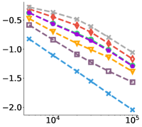
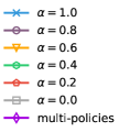
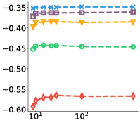
number of transitions, $n$	Trajectory length $T$	Trajectory length $T$
(a) Varying $n$, $\alpha$, fixed $\gamma=0.95$	(b) Varying $n$, $T$, fixed $\gamma=0.95$	(c)Varying $n$, $\alpha$, fixed $\gamma=0.99$

Figure 5: Ablation studies on the data collection procedure, as we (a) change the behavior policies, and (b)-(c) change the trajectory lengths. The other settings are the same as that in Figure 3.

H.3 Sensitivity to the Data Collection Procedure

We investigate the sensitivity of our method as we use different behavior policies to collect the dataset $\hat{\mathsf{D}}_{n}$.

Varying Behavior Policies

We study the effect of using different behavior policies. We consider the following cases:

1. Data is collected from a single behavior policy of form $\pi_{\alpha}=\alpha\pi+(1-\alpha)\pi_{0}$, where $\pi$ is the target policy and $\pi_{0}$ is another policy. We construct $\pi$ and $\pi_{0}$ to be Gaussian policies of form $\pi(a|s)\propto\exp(f(s,a)/\tau)$ with different temperature $\tau$, where temperature for target policy is $\tau=0.1$ and temperature for $\pi_{0}$ is $\tau=1$.

2. The dataset $\hat{\mathsf{D}}_{n}$ is the combination of the data collected from multiple behavior policies of form $\pi_{\alpha}$ defined as above, with $\alpha\in\{{0.0},{0.2},{0.4},{0.6},{0.8}\}$.

We show in Figure 5(a) that the length of the confidence intervals by our method as we vary the number $n$ of transition pairs and the mixture rate $\alpha$. We can see that the length of the interval decays with the sample size $n$ for all mixture rate $\alpha$. Larger $\alpha$ yields better performance because the behavior policies are closer to the target policy.

Varying Trajectory Length $T$ in $\hat{\mathsf{D}}_{n}$

As we collect $\hat{\mathsf{D}}_{n}$, we can either have a small number of long trajectories, or a larger number of short trajectories. In Figure 5(b)-(c), we vary the length $T$ of the trajectories as we collect $\hat{\mathsf{D}}_{n}$, while fixing the total number $n$ of transition pairs. In this way, the number of trajectories in each $\hat{\mathsf{D}}_{n}$ would be $m=n/T$. We can see that the trajectory length does not impact the results significantly, especially when the length is reasonably large (e.g., $T\geq 20$).

Appendix I Finite Horzion and Time-varying MDPs

In this paper we mainly focus on infinite-horizion and time-homogeneous MDPs. Here we consider how to extend our method to finite-horizon and time-inhomogeneous MDPs, where the transition probability and reward are time-dependent and we have a finite horizon length $H<+\infty$. That is, we consider cases when the next state and reward follow an unknown, time-dependent transition distribution,

$$(r_{t},s_{t+1})\sim\mathsf{P}(\cdot|s_{t},a_{t};~{}~{}t),$$

and we want to estimate the following finite-horizon expected reward

$$J_{\pi,P,H}=\mathbb{E}_{\pi,\mathsf{P}}\left[\sum_{t=0}^{H-1}\gamma^{t}r_{t}~{}|~{}s_{0}\sim\mathsf{D}_{0}\right],$$

where the horizon length $H$ is finite but can be large. We should distinguish $H$ (which is a part of the problem definition) with the trajectory length $T$ of the data in $\hat{\mathsf{D}}_{n}$ (which is a part of the data collection procedure).

We can approach this problem by transforming it into an infinite-horizon and time-homogeneous problem and then apply our method. This can be done by incoporating the time $t$ as a part of the state vector. To be concrete, assume we collect a set of transition pairs $(s_{i},a_{i},r_{i},s_{i}^{\prime},t_{i})_{i=1}^{n}$, where in addition to $(s_{i},a_{i},r_{i},s_{i}^{\prime})$, we also record the time $t_{i}$ when the transition occurs. We define an augmented state $\bar{s}_{i}=[s_{i},t_{i}]$ and $\bar{s}_{i}^{\prime}=[s_{i},t_{i}+1]$ which include the time $t_{i}$ as a part. Our method can be then applied without modification on the augmented dataset $\{\bar{s}_{i},a_{i},r_{i}\}_{i=1}^{n}$, once we ensure that $q([s,t],a)=0$ for all $t\geq H$ when defining the function set $\mathcal{Q}$. To build an RKHS $\mathcal{Q}$ that satisfy $q([s,t],a)=0,~{}\forall t\geq H,~{}q\in\mathcal{Q}$, we just need to use a kernel $\tilde{k}([s,a,t],[s^{\prime},a^{\prime},t^{\prime}])$ such that $\tilde{k}([s,a,t],[s^{\prime},a^{\prime},t^{\prime}])=0$ whenever $t\geq H$ or $t^{\prime}\geq H$.

References

- Arlot et al. (2010) Sylvain Arlot, Gilles Blanchard, Etienne Roquain, et al. Some nonasymptotic results on resampling in high dimension, I: confidence regions. The Annals of Statistics, 38(1):51–82, 2010.
- Asadi et al. (2018) Kavosh Asadi, Evan Cater, Dipendra Misra, and Michael L Littman. Equivalence between wasserstein and value-aware loss for model-based reinforcement learning. arXiv preprint arXiv:1806.01265, 2018.
- Bellemare et al. (2017) Marc G Bellemare, Will Dabney, and Rémi Munos. A distributional perspective on reinforcement learning. In International Conference on Machine Learning, pages 449–458, 2017.
- Brockman et al. (2016) Greg Brockman, Vicki Cheung, Ludwig Pettersson, Jonas Schneider, John Schulman, Jie Tang, and Wojciech Zaremba. Openai gym. arXiv preprint arXiv:1606.01540, 2016.
- Dai et al. (2020) Bo Dai, Ofir Nachum, Yinlam Chow, Lihong Li, Csaba Szepesvári, and Dale Schuurmans. Coindice: Off-policy confidence interval estimation. In Advances in Neural Information Processing Systems, 2020.
- Duan et al. (2020) Yaqi Duan, Zeyu Jia, and Mengdi Wang. Minimax-optimal off-policy evaluation with linear function approximation. In International Conference on Machine Learning, 2020.
- Engel et al. (2005) Yaakov Engel, Shie Mannor, and Ron Meir. Reinforcement learning with Gaussian processes. In Proceedings of the 22nd international conference on Machine learning, pages 201–208, 2005.
- Feng et al. (2019) Yihao Feng, Lihong Li, and Qiang Liu. A kernel loss for solving the Bellman equation. In Advances in Neural Information Processing Systems, pages 15456–15467, 2019.
- Feng et al. (2020) Yihao Feng, Tongzheng Ren, Ziyang Tang, and Qiang Liu. Accountable off-policy evaluation with kernel Bellman statistics. In International Conference on Machine Learning, 2020.
- Feng et al. (2021) Yihao Feng, Ziyang Tang, Na Zhang, and Qiang Liu. Non-asymptotic confidence intervals of off-policy evaluation: Primal and dual bounds. In International Conference on Learning Representations, 2021.
- Fonteneau et al. (2013) Raphael Fonteneau, Susan A. Murphy, Louis Wehenkel, and Damien Ernst. Batch mode reinforcement learning based on the synthesis of artificial trajectories. Annals of Operations Research, 208(1):383–416, 2013.
- Ghavamzadeh et al. (2016) Mohammad Ghavamzadeh, Shie Mannor, Joelle Pineau, and Aviv Tamar. Bayesian reinforcement learning: A survey. arXiv preprint arXiv:1609.04436, 2016.
- Hanna et al. (2017) Josiah P Hanna, Peter Stone, and Scott Niekum. Bootstrapping with models: Confidence intervals for off-policy evaluation. In Thirty-First AAAI Conference on Artificial Intelligence, 2017.
- Hao et al. (2021) Botao Hao, Yaqi Duan, Hao Lu, Csaba Szepesvári, Mengdi Wang, et al. Bootstrapping statistical inference for off-policy evaluation. arXiv preprint arXiv:2102.03607, 2021.
- Jiang and Huang (2020) Nan Jiang and Jiawei Huang. Minimax confidence interval for off-policy evaluation and policy optimization. In Advances in Neural Information Processing Systems, 2020.
- Jiang and Li (2016) Nan Jiang and Lihong Li. Doubly robust off-policy evaluation for reinforcement learning. In Proceedings of the 23rd International Conference on Machine Learning, pages 652–661, 2016.
- Kostrikov and Nachum (2020) Ilya Kostrikov and Ofir Nachum. Statistical bootstrapping for uncertainty estimation in off-policy evaluation. arXiv preprint arXiv:2007.13609, 2020.
- Lahiri (2013) Soumendra Nath Lahiri. Resampling methods for dependent data. Springer Science & Business Media, 2013.
- Lazic et al. (2020) Nevena Lazic, Dong Yin, Mehrdad Farajtabar, Nir Levine, Dilan Gorur, Chris Harris, and Dale Schuurmans. A maximum-entropy approach to off-policy evaluation in average-reward MDPs. In Advances in Neural Information Processing Systems, 2020.
- Liu et al. (2018a) Qiang Liu, Lihong Li, Ziyang Tang, and Dengyong Zhou. Breaking the curse of horizon: Infinite-horizon off-policy estimation. In Advances in Neural Information Processing Systems, pages 5356–5366, 2018a.
- Liu et al. (2018b) Yao Liu, Omer Gottesman, Aniruddh Raghu, Matthieu Komorowski, Aldo A. Faisal, Finale Doshi-Velez, and Emma Brunskill. Representation balancing MDPs for off-policy policy evaluation. In Advances in Neural Information Processing Systems 31 (NeurIPS), pages 2649–2658, 2018b.
- Liu et al. (2020) Yao Liu, Pierre-Luc Bacon, and Emma Brunskill. Understanding the curse of horizon in off-policy evaluation via conditional importance sampling. In International Conference on Machine Learning, 2020.
- Mousavi et al. (2020) Ali Mousavi, Lihong Li, Qiang Liu, and Denny Zhou. Black-box off-policy estimation for infinite-horizon reinforcement learning. In International Conference on Learning Representations, 2020.
- Murphy et al. (2001) Susan A. Murphy, Mark van der Laan, and James M. Robins. Marginal mean models for dynamic regimes. Journal of the American Statistical Association, 96(456):1410–1423, 2001.
- Nachum et al. (2019a) Ofir Nachum, Yinlam Chow, Bo Dai, and Lihong Li. Dualdice: Behavior-agnostic estimation of discounted stationary distribution corrections. In Advances in Neural Information Processing Systems, pages 2318–2328, 2019a.
- Nachum et al. (2019b) Ofir Nachum, Bo Dai, Ilya Kostrikov, Yinlam Chow, Lihong Li, and Dale Schuurmans. Algaedice: Policy gradient from arbitrary experience. arXiv preprint arXiv:1912.02074, 2019b.
- Nesterov (2003) Yurii Nesterov. Introductory lectures on convex optimization: A basic course, volume 87. Springer Science & Business Media, 2003.
- Paulin (2015) Daniel Paulin. Concentration inequalities for markov chains by marton couplings and spectral methods. Electron. J. Probab, 20(79):1–32, 2015.
- Pinelis (1992) Iosif Pinelis. An approach to inequalities for the distributions of infinite-dimensional martingales. In Probability in Banach Spaces, 8: Proceedings of the Eighth International Conference, pages 128–134. Springer, 1992.
- Precup (2000) Doina Precup. Eligibility traces for off-policy policy evaluation. Computer Science Department Faculty Publication Series, page 80, 2000.
- Precup (2001) Doina Precup. Temporal abstraction in reinforcement learning. ProQuest Dissertations and Theses, 2001.
- Precup et al. (2000) Doina Precup, Richard S. Sutton, and Satinder P. Singh. Eligibility traces for off-policy policy evaluation. In Proceedings of the 17th International Conference on Machine Learning, pages 759–766, 2000.
- Rahimi and Recht (2007) Ali Rahimi and Benjamin Recht. Random features for large-scale kernel machines. In Advances in neural information processing systems, pages 1177–1184, 2007.
- Rakhlin et al. (2015) Alexander Rakhlin, Karthik Sridharan, and Ambuj Tewari. Sequential complexities and uniform martingale laws of large numbers. Probability Theory and Related Fields, 161(1-2):111–153, 2015.
- Rosasco et al. (2010) Lorenzo Rosasco, Mikhail Belkin, and Ernesto De Vito. On learning with integral operators. Journal of Machine Learning Research, 11(2), 2010.
- Scholkopf and Smola (2018) Bernhard Scholkopf and Alexander J Smola. Learning with kernels: support vector machines, regularization, optimization, and beyond. Adaptive Computation and Machine Learning series, 2018.
- Schulman et al. (2017) John Schulman, Filip Wolski, Prafulla Dhariwal, Alec Radford, and Oleg Klimov. Proximal policy optimization algorithms. arXiv preprint arXiv:1707.06347, 2017.
- Sutton and Barto (1998) Richard S. Sutton and Andrew G. Barto. Reinforcement Learning: An Introduction. MIT Press, Cambridge, MA, March 1998. ISBN 0-262-19398-1.
- Tang et al. (2020a) Ziyang Tang, Yihao Feng, Lihong Li, Dengyong Zhou, and Qiang Liu. Doubly robust bias reduction in infinite horizon off-policy estimation. In International Conference on Learning Representations (ICLR), 2020a.
- Tang et al. (2020b) Ziyang Tang, Yihao Feng, Na Zhang, Jian Peng, and Qiang Liu. Off-policy interval estimation with lipschitz value iteration. In Advances in Neural Information Processing Systems, 2020b.
- Thomas (2015) Philip S Thomas. Safe reinforcement learning. PhD thesis, University of Massachusetts, 2015.
- Thomas and Brunskill (2016) Philip S. Thomas and Emma Brunskill. Data-efficient off-policy policy evaluation for reinforcement learning. In Proceedings of the 33rd International Conference on Machine Learning, pages 2139–2148, 2016.
- Thomas et al. (2015a) Philip S. Thomas, Georgios Theocharous, and Mohammad Ghavamzadeh. High confidence policy improvement. In Proceedings of the 32nd International Conference on Machine Learning, pages 2380–2388, 2015a.
- Thomas et al. (2015b) Philip S Thomas, Georgios Theocharous, and Mohammad Ghavamzadeh. High-confidence off-policy evaluation. In Twenty-Ninth AAAI Conference on Artificial Intelligence, 2015b.
- Uehara et al. (2020) Masatoshi Uehara, Jiawei Huang, and Nan Jiang. Minimax weight and q-function learning for off-policy evaluation. Proceedings of the 37th International Conference on Machine Learning, 2020.
- Wen et al. (2020) Junfeng Wen, Bo Dai, Lihong Li, and Dale Schuurmans. Batch stationary distribution estimation. In International Conference on Machine Learning, 2020.
- White and White (2010) Martha White and Adam White. Interval estimation for reinforcement-learning algorithms in continuous-state domains. In Advances in Neural Information Processing Systems, pages 2433–2441, 2010.
- Xie and Jiang (2020) Tengyang Xie and Nan Jiang. Q* approximation schemes for batch reinforcement learning: A theoretical comparison. In Conference on Uncertainty in Artificial Intelligence (UAI), 2020.
- Xie et al. (2019) Tengyang Xie, Yifei Ma, and Yu-Xiang Wang. Towards optimal off-policy evaluation for reinforcement learning with marginalized importance sampling. In Advances in Neural Information Processing Systems, pages 9668–9678, 2019.
- Yang et al. (2020a) Mengjiao Yang, Bo Dai, Ofir Nachum, George Tucker, and Dale Schuurmans. Offline policy selection under uncertainty. arXiv preprint arXiv:2012.06919, 2020a.
- Yang et al. (2020b) Mengjiao Yang, Ofir Nachum, Bo Dai, Lihong Li, and Dale Schuurmans. Off-policy evaluation via the regularized Lagrangian. In Advances in Neural Information Processing Systems, 2020b.
- Yin and Wang (2020) Ming Yin and Yu-Xiang Wang. Asymptotically efficient off-policy evaluation for tabular reinforcement learning. In Proceedings of the International Conference on Artificial Intelligence and Statistics (AISTATS), 2020.
- Yin et al. (2020) Ming Yin, Yu Bai, and Yu-Xiang Wang. Near optimal provable uniform convergence in off-policy evaluation for reinforcement learning. arXiv preprint arXiv:2007.03760, 2020.
- Zhang et al. (2020a) Ruiyi Zhang, Bo Dai, Lihong Li, and Dale Schuurmans. Gendice: Generalized offline estimation of stationary values. In International Conference on Learning Representations, 2020a.
- Zhang et al. (2020b) Shangtong Zhang, Bo Liu, and Shimon Whiteson. Gradientdice: Rethinking generalized offline estimation of stationary values. In International Conference on Machine Learning, 2020b.