Multiple Zeros of Nonlinear Systems

Barry H. Dayton Department of Mathematics, Northeastern Illinois University, Chicago, IL 60625 (email: bhdayton@neiu.edu).    Tien-Yien Li Department of Mathematics, Michigan State University, East Lansing, MI 48824 (li@math.msu.edu). Research supported in part by NSF under Grant DMS-0811172.    Zhonggang Zeng Department of Mathematics, Northeastern Illinois University, Chicago, IL 60625 (zzeng@neiu.edu). Research supported in part by NSF under Grant DMS-0715127.
Abstract

As an attempt to bridge between numerical analysis and algebraic geometry, this paper formulates the multiplicity for the general nonlinear system at an isolated zero, presents an algorithm for computing the multiplicity structure, proposes a depth-deflation method for accurate computation of multiple zeros, and introduces the basic algebraic theory of the multiplicity.  Furthermore, this paper elaborates and proves some fundamental properties of the multiplicity, including local finiteness, consistency, perturbation invarance, and depth-deflatability.  As a justification of this formulation, the multiplicity is proved to be consistent with the multiplicity defined in algebraic geometry for the special case of polynomial systems.  The proposed algorithms can accurately compute the multiplicity and the multiple zeros using floating point arithmetic even if the nonlinear system is perturbed.

2000 Mathematics Subject Classification:  Primary 65H10,  Secondary 68W30

1 Introduction

Solving a system of nonlinear equations in the form  $\mathbf{f}(\mathbf{x})\,=\,\mathbf{0}$,  or

$$f_{1}(x_{1},\ldots,x_{s})~{}~{}=~{}~{}f_{2}(x_{1},\ldots,x_{s})~{}~{}=~{}~{}\cdots~{}~{}=~{}~{}f_{t}(x_{1},\ldots,x_{s})~{}~{}=~{}~{}0$$ (1)

with  $\mathbf{f}=[f_{1},\ldots,f_{t}]^{{\mbox{\tiny$\mathsf{H}$}}}$  and  $\mathbf{x}=(x_{1},\ldots,x_{s})$,  is one of the most fundamental problems in scientific computing, and one of the main topics in most numerical analysis textbooks.  In the literature outside of algebraic geometry, however, an important question as well as its answer seem to be absent over the years:  What is the multiplicity of an isolated zero to the system and how to identify it accurately.

For a single equation  $f(x)=0$,  it is well known that the multiplicity of a zero  $x_{*}$  is  $m$  if

$$f(x_{*})~{}=~{}f^{\prime}(x_{*})~{}=~{}\cdots~{}=~{}f^{(m\mbox{\footnotesize-}1)}(x_{*})~{}~{}=~{}~{}0~{}~{}~{}~{}\mbox{and}~{}~{}~{}f^{(m)}(x_{*})~{}\neq~{}0.$$ (2)

The multiplicity of a polynomial system at a zero has gone through rigorous formulations since Newton’s era [8, pp. 127-129] as one of the oldest subjects of algebraic geometry.  Nonetheless, the standard multiplicity formulation and identification via Gröbner bases for polynomial systems are somewhat limited to symbolic computation, and largely unknown to numerical analysts.

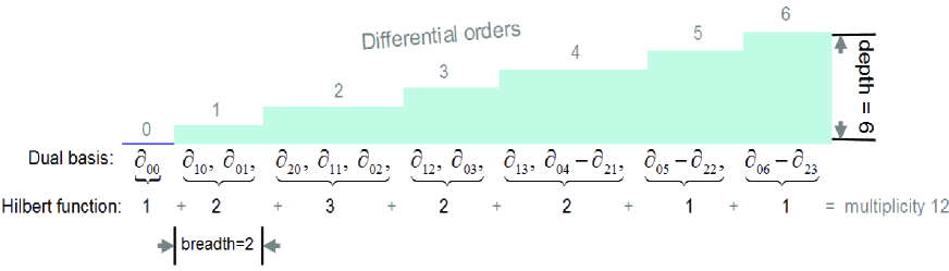
As an attempt to bridge between algebraic geometry and numerical analysis, we propose a rigorous formulation for the multiplicity structure of a general nonlinear system at a zero.  This multiplicity structure includes, rather than just a single integer for the multiplicity, several structural invariances that are essential in providing characteristics of the system and accurate computation of the zero.  For instance, at the zero  $\mathbf{x}_{*}=(0,0)$  of the nonlinear system

$$\sin x_{1}\cos x_{1}-x_{1}~{}~{}=~{}~{}\sin x_{2}\sin^{2}x_{1}+x_{2}^{4}~{}~{}=~{}~{}0$$ (3)

we shall have:

  • The multiplicity  $m=12$.

  • Under a small perturbation to the system (3), there is a cluster of exactly 12 zeros (counting multiplicities) in a neighborhood of  $\mathbf{x}_{*}=(0,0)$.

  • The Hilbert function  $\{1,2,3,2,2,1,1,0,0,\cdots\}$  forms a partition of the multiplicity  $12$.

  • There exist 12 linearly independent differential operators  ${\partial}_{00},~{}{\partial}_{10},~{}\ldots,~{}{\partial}_{05}-{\partial}_{22},~{}{\partial}_{06}-{\partial}_{23}$, grouped by the differential orders and counted by the Hilbert function as shown in Figure 1 below.  They induce 12 differential functionals that span the dual space associated with system (3).  These functionals satisfy a closedness condition and vanish on the two functions in (3) at the zero $(0,0)$.  Here, the differential operator

    $${\partial}_{j_{1}\cdots j_{s}}~{}~{}\equiv~{}~{}{\partial}_{x_{1}^{j_{1}}\cdots x_{s}^{j_{s}}}~{}~{}\equiv~{}~{}\mbox{\footnotesize$\displaystyle\frac{1}{j_{1}!\cdots j_{s}!}\;\;\frac{{\partial}^{j_{1}+\cdots+j_{s}}}{{\partial}x_{1}^{j_{1}}\cdots{\partial}x_{s}^{j_{s}}}$}$$ (4)

    of order  $j_{1}+\cdots+j_{s}$  naturally induces a linear functional

    $${\partial}_{j_{1}\cdots j_{s}}[\mathbf{x}_{*}]~{}:~{}f~{}\longrightarrow({\partial}_{j_{1}\cdots j_{s}}f)(\mathbf{x}_{*})$$ (5)

    on functions  $f$  whose indicated partial derivative exists at the zero  $\mathbf{x}_{*}$.

  • The breadth, or the nullity of the Jacobian at  $\mathbf{x}_{*}$,  is  2.

  • The depth, which is the highest differential order of the functionals at  $\mathbf{x}_{*}$,  is  6.

Refer to caption
Figure 1: Illustration of the multiplicity structure including dual basis, Hilbert function, breadth and depth of the system (3) at the zero  $(0,0)$

Such a multiplicity structure at an isolated zero of a general nonlinear system will be introduced in §2.  We prove the so-defined multiplicity agrees with the intersection multiplicity of polynomial systems in algebraic geometry.  It is finite if and only if the zero is isolated, and more importantly, this finiteness ensures termination of the multiplicity identification algorithm NonlinearSystemMultiplicity given in §2.3, and it also provides a mechanism for determining whether a zero is isolated [2].  Furthermore, the multiplicity structure of the given nonlinear system can be computed by constructing the Macaulay matrices [21] together with the numerical rank revealing [20].  As a result, we developed numerical algorithms that accurately calculate the multiplicity structure even if the system data are inexact at a zero that is given approximately (c.f. §2.3 and §3.3).

It is well documented that multiple zeros are difficult to compute accurately even for a single equation.  There is a perceived barrier of “attainable accuracy”: The number of correct digits attainable for a multiple zero is bounded by the number of digits in the hardware precision divided by the multiplicity.  For instance, only three correct digits can be expected in computing a five-fold zero using the double precision (16 digits) floating point arithmetic.  Such a barrier has been overcome for univariate polynomial equations [34].  Based on the multiplicity theory established in this article, we shall derive a depth-deflation algorithm in §3 for computing multiple zeros of general nonlinear systems, which can accurately compute the multiple zeros without extending the arithmetic precision even when the nonlinear system is perturbed.  The depth defined in the multiplicity structure actually bounds the number of deflation steps.  A related multiplicity deflation method is used in [17], in which the main goal is to speed up Newton’s iteration.

As mentioned above, the study of the multiplicity for a polynomial system at an isolated zero can be traced back to Newton’s time [8, pp. 127-129].  Besides polynomial systems, multiple zeros of a nonlinear system occur frequently in scientific computing.  For instance, when a system depends on certain parameters, a multiple zero emerges when the parameters reach a bifurcation point [3, §1.1].  Accurate computation of the multiple zero and reliable identification of the multiplicity structure may have a profound ramification in scientific computing.  This paper furnishes the theoretical details of the preliminary results on polynomial systems announced in an abstract [5], and in addition, the scope of this work has been substantially expanded to general nonlinear systems.

2 Formulation and computation of the multiplicity structure

2.1 The notion and fundamental theorems of the multiplicity

The general nonlinear system (1) is represented by either the mapping  $\mathbf{f}\,:\,\mathbbm{C}^{s}\longrightarrow\mathbbm{C}^{t}$  or the set  $F=\{f_{1},\ldots,f_{t}\}$  of functions in the variables  $x_{1},\ldots,x_{s}$.  We assume functions  $f~{}:~{}\mathbbm{C}^{s}\longrightarrow\mathbbm{C}$  in this paper have all the relevant partial derivatives arising in the elaboration.  The multiplicity which we shall formulate in this section will extend both the multiplicity (2) of a single equation and the Macaulay-Gröbner duality formulation of multiplicity for polynomial systems.

Denote  $\N=\{0,\pm 1,\pm 2,\ldots\}$.  For an integer array  $\mathbf{j}=(j_{1},\ldots,j_{s})\in\N^{s}$,  write  $\mathbf{j}\geq 0$  if  $j_{i}\geq 0$  for all  $i\in\{1,\ldots,s\}$.  For every  $\mathbf{j}=(j_{1},\cdots,j_{s})\in\N^{s}$  with  $\mathbf{j}\geq 0$,  denote  $\mathbf{x}^{\mathbf{j}}=x_{1}^{j_{1}}\cdots x_{s}^{j_{s}}$  and  $(\mathbf{x}-\mathbf{y})^{\mathbf{j}}=(x_{1}-y_{1})^{j_{1}}\cdots(x_{s}-y_{s})^{j_{s}}$,  and differential functional monomial  ${\partial}_{\mathbf{j}}[{\hat{\mathbf{x}}}]$  at  ${\hat{\mathbf{x}}}\in\mathbbm{C}^{s}$  as in (5), with order  $|\mathbf{j}|=j_{1}+\cdots+j_{s}$.  For simplicity, we adopt the convention

$${\partial}_{\mathbf{j}}[{\hat{\mathbf{x}}}](f)~{}~{}\equiv~{}~{}0~{}~{}~{}~{}\mbox{for all ~{}$f$ ~{}whenever}~{}~{}~{}\mathbf{j}\not\geq 0$$ (6)

throughout this paper.  A linear combination  $c=c_{\mathbf{j}_{1}}{\partial}_{\mathbf{j}_{1}}[{\hat{\mathbf{x}}}]+\cdots+c_{\mathbf{j}_{k}}{\partial}_{\mathbf{j}_{k}}[{\hat{\mathbf{x}}}]$  is called a differential functional, which will produce a set of numbers  $c(F)=\{c(f_{1}),\ldots,c(f_{t})\}$  when applied to the system  $F=\{f_{1},\ldots,f_{t}\}$.  For differential functionals, the linear anti-differentiation transformation  $\phi_{i}$  is defined by  $\phi_{i}\big{(}\sum_{\mathbf{j}}c_{\mathbf{j}}{\partial}_{\mathbf{j}}[{\hat{\mathbf{x}}}]\big{)}~{}=~{}\sum_{\mathbf{j}}c_{\mathbf{j}}\phi_{i}\big{(}{\partial}_{\mathbf{j}}[{\hat{\mathbf{x}}}]\big{)}$  with

$$\phi_{i}\big{(}{\partial}_{j_{1}\ldots j_{s}}[{\hat{\mathbf{x}}}]\big{)}~{}~{}=~{}~{}{\partial}_{j^{\prime}_{1}\ldots j^{\prime}_{s}}[{\hat{\mathbf{x}}}]~{}~{}~{}~{}~{}\mbox{where}~{}~{}~{}~{}~{}j^{\prime}_{\sigma}~{}~{}=~{}~{}\left\{\begin{array}[]{cc}j_{i}&\mbox{if ~{}$\sigma\neq i$}\\ j_{i}\!-\!1&\mbox{if ~{}$\sigma=i$}\end{array}\right.$$ (7)

for  $i=1,\ldots,s$.  From (6), we have  $\phi_{i}({\partial}_{\mathbf{j}}[{\hat{\mathbf{x}}}])=0$  if  $j_{i}=0$.  With these differential functionals and the linear transformations, we now formulate the multiplicity at a zero  ${\hat{\mathbf{x}}}$  of the nonlinear system (1) as follows.

Definition 1

Let  $F=\{f_{1},\ldots,f_{t}\}$  be a system of functions having derivatives of order  $\gamma\geq 1$  at a zero  ${\hat{\mathbf{x}}}\in\mathbbm{C}^{s}$.  Let  ${\cal D}_{\hat{\mathbf{x}}}^{0}(F)\,=\,\mathpzc{span}\{{\partial}_{0\ldots 0}\}$  and

$\displaystyle{\cal D}_{{\hat{\mathbf{x}}}}^{\alpha}(F)\;=\;\Big{\{}\,c=\sum_{\mathbf{j}\in\N^{s},\,c_{\mathbf{j}}\in\mathbbm{C},\,|\mathbf{j}|\leq\alpha}c_{\mathbf{j}}{\partial}_{\mathbf{j}}[{\hat{\mathbf{x}}}]\;\Big{|}\;c(F)=\{0\},~{}\phi_{i}(c)\in{\cal D}_{{\hat{\mathbf{x}}}}^{\alpha\mbox{\footnotesize-}1}(F),~{}~{}\forall~{}i=1,\dots,s\Big{\}}$ (8)

for  $\alpha=1,\ldots,\gamma$.  We call such sets dual subspaces.  If  ${\cal D}_{\hat{\mathbf{x}}}^{\gamma}(F)={\cal D}_{\hat{\mathbf{x}}}^{\gamma\mbox{\footnotesize-}1}(F)$,  then the vector space

$${\cal D}_{\hat{\mathbf{x}}}(F)~{}~{}=~{}~{}{\cal D}_{\hat{\mathbf{x}}}^{0}(F)\,\cup\,{\cal D}_{\hat{\mathbf{x}}}^{1}(F)\,\cup\,\cdots\,\cup\,{\cal D}_{\hat{\mathbf{x}}}^{\gamma-1}(F)~{}~{}=~{}~{}{\cal D}_{\hat{\mathbf{x}}}^{\gamma}(F)$$ (9)

is called the  dual space of the system  $F$  at  ${\hat{\mathbf{x}}}$.  The dimension of  ${\cal D}_{\hat{\mathbf{x}}}(F)$, i.e.  $\mathpzc{dim}\big{(}{\cal D}_{\hat{\mathbf{x}}}(F)\big{)}$,  is called the  multiplicity of  $F$  at  ${\hat{\mathbf{x}}}$.

Notice that dual subspaces  ${\cal D}_{\hat{\mathbf{x}}}^{\alpha}(F)$’s strictly enlarge as the differential order  $\alpha$  increases until reaching certain  $\alpha=\delta$  at which  ${\cal D}_{\hat{\mathbf{x}}}^{\delta}(F)={\cal D}_{\hat{\mathbf{x}}}^{\delta\mbox{\raisebox{-1.20552pt}{\tiny${}^{+}$}}1}(F)$,  and thus all functionals in  ${\cal D}_{\hat{\mathbf{x}}}^{\delta\mbox{\raisebox{-1.20552pt}{\tiny${}^{+}$}}1}(F)$  are of  differential orders up to  $\delta$.  As a result, there are no functionals in the subsequent dual subspaces with differential orders  $\delta+2,\,\delta+3,\ldots$  since  $\phi_{i}\big{(}{\cal D}_{\hat{\mathbf{x}}}^{\alpha}(F)\big{)}\subset{\cal D}_{\hat{\mathbf{x}}}^{\alpha\mbox{\raisebox{-1.20552pt}{\tiny${}^{+}$}}1}(F)$  for  $i=1,\ldots,s$.  Thus

$${\cal D}_{\hat{\mathbf{x}}}^{0}(F)~{}\subsetne~{}{\cal D}_{\hat{\mathbf{x}}}^{1}(F)~{}\subsetne~{}\cdots~{}\subsetne{\cal D}_{\hat{\mathbf{x}}}^{\delta}(F)~{}=~{}{\cal D}_{\hat{\mathbf{x}}}^{\delta\mbox{\raisebox{-1.20552pt}{\tiny${}^{+}$}}1}(F)~{}=~{}\cdots~{}=~{}{\cal D}_{\hat{\mathbf{x}}}^{\gamma}(F)~{}=~{}{\cal D}_{\hat{\mathbf{x}}}(F).$$

The integer  $\delta$,  called the depth which will be defined later, is the highest order of differential functionals in the dual space.

We may also denote the dual space as  ${\cal D}_{\hat{\mathbf{x}}}(\mathbf{f})$  when the nonlinear system is represented as a mapping  $\mathbf{f}=[f_{1},\ldots,f_{t}]^{\top}$.  It is important to note that vanishing at the system  $c(F)=\{0\}$  is insufficient for the functional  $c$  to be in the dual space  ${\cal D}_{\hat{\mathbf{x}}}(F)$.  This becomes more transparent in single equation  $f(x)=0$  where the multiplicity is not the number of vanishing derivatives  $f^{(k)}(x)=0$  at a zero  $x_{*}$.  For instance, infinite number of functionals  ${\partial}_{0}[0],~{}{\partial}_{2}[0],~{}{\partial}_{4}[0],~{}\ldots$  vanish at the  $(1\times 1)$-system  $\{\sin x\}$,  since derivatives  $\sin^{(2k)}0=0$  for all integers  $k\geq 0$.  Among these functionals, however, only  ${\partial}_{0}[0]\in{\cal D}_{0}(\{\sin x\})$  since

$$\phi_{1}({\partial}_{2k}[0])(\sin x)~{}~{}=~{}~{}{\partial}_{2k-1}[0](\sin x)~{}~{}=~{}~{}\mbox{$\frac{(-1)^{k\mbox{\footnotesize-}1}}{(2k-1)!}$}\cos 0~{}~{}\neq~{}~{}0,$$

namely  ${\partial}_{2k}[0]\not\in{\cal D}_{0}(\{\sin x\})$  for all  $k\geq 1$,  therefore the multiplicity of  $\sin x$  is one at  $x=0$.  The crucial closedness condition

$$\phi_{i}(c)~{}~{}\in~{}~{}{\cal D}_{\hat{\mathbf{x}}}(F)~{}~{}~{}~{}\mbox{for all}~{}~{}~{}~{}c\in{\cal D}_{\hat{\mathbf{x}}}(F)~{}~{}\mbox{and}~{}~{}i=1,\ldots,s$$ (10)

in Definition 1 requires the dual space  ${\cal D}_{\hat{\mathbf{x}}}(F)$  to be invariant under the anti-differentiation transformation  $\phi_{i}$’s.  The following lemma is a direct consequence of the closedness condition.

Lemma 1

A differential functional  $c$  is in the dual space  ${\cal D}_{\hat{\mathbf{x}}}(F)$  of the nonlinear system  $F=\{f_{1},\ldots,f_{t}\}$  at the zero  ${\hat{\mathbf{x}}}$  if and only if

$$c\big{(}(\mathbf{x}-{\hat{\mathbf{x}}})^{\mathbf{j}}f_{i}(\mathbf{x})\big{)}~{}~{}=~{}~{}0~{}~{}~{}~{}\mbox{for any}~{}~{}~{}~{}i\in\{1,\ldots,t\}~{}~{}~{}~{}\mbox{and}~{}~{}~{}~{}\mathbf{j}\in\N^{s}~{}~{}~{}\mbox{with}~{}~{}~{}\mathbf{j}\geq 0.$$ (11)

Proof.   For any  $\mathbf{j}=(j_{1},\ldots,j_{s})$,  $\mathbf{k}=(k_{1},\ldots,k_{s})$,  and function  $f$,  the Leibniz rule of derivatives yields

$${\partial}_{\mathbf{j}}[{\hat{\mathbf{x}}}]\big{(}(\mathbf{x}-{\hat{\mathbf{x}}})^{\mathbf{k}}f(\mathbf{x})\big{)}~{}~{}=~{}~{}{\partial}_{\mathbf{j}\mbox{\footnotesize-}\mathbf{k}}[{\hat{\mathbf{x}}}](f)~{}~{}\equiv~{}~{}\big{(}\phi_{1}^{k_{1}}\circ\phi_{2}^{k_{2}}\circ\cdots\circ\phi_{s}^{k_{s}}\big{)}({\partial}_{\mathbf{j}}[{\hat{\mathbf{x}}}])(f).$$ (12)

The equation (11) holds because of the closedness condition (10) and the linearity of  $c$.   $\Box$

The dual space  ${\cal D}_{\hat{\mathbf{x}}}(F)$  itself actually contains more structural invariants of the multiple zero beyond the multiplicity for the system $F$.  Via dual subspaces  ${\cal D}_{\hat{\mathbf{x}}}^{\alpha}(F)$,  a Hilbert function  $\mathrm{h}:\N\rightarrow\N$  can be defined as follows:

$$\mathrm{h}(0)~{}=~{}\mathpzc{dim}\big{(}{\cal D}^{0}_{{\hat{\mathbf{x}}}}(F)\big{)}\equiv 1,~{}~{}~{}~{}\mathrm{h}(\alpha)~{}=~{}\mathpzc{dim}\big{(}{\cal D}^{\alpha}_{{\hat{\mathbf{x}}}}(F)\big{)}-\mathpzc{dim}\big{(}{\cal D}^{\alpha-1}_{{\hat{\mathbf{x}}}}(F)\big{)}\;\;\mbox{\ \ for \ }\alpha\in\{\,1,2,\dots\,\}.$$ (13)

This Hilbert function is often expressed as a infinite sequence  $\{\mathrm{h}(0),\mathrm{h}(1),\ldots\}$,  with which we introduce the breadth and the depth of  ${\cal D}_{{\hat{\mathbf{x}}}}(F)$,  denoted by  $\beta_{{\hat{\mathbf{x}}}}(F)$ and $\delta_{{\hat{\mathbf{x}}}}(F)$  respectively, as

$$\beta_{{\hat{\mathbf{x}}}}(F)\;=\;\mathrm{h}\,(1)\mbox{ \ \ and \ \ }\delta_{{\hat{\mathbf{x}}}}(F)\;=\;\max\{\,\alpha\;|\;\mathrm{h}\,(\alpha)>0\,\}.$$

In other words, the breadth is the nullity of the Jacobian at  ${\hat{\mathbf{x}}}$  for the system (1) and the depth is the highest differential order of functionals in  ${\cal D}_{\hat{\mathbf{x}}}(F)$.  They are important components of the multiplicity structure that dictate the deflation process for accurate computation of the multiple zero (c.f. §3).

In contrast to system (3), the system  $\{x_{1}^{2}\sin x_{1},~{}x_{2}^{2}-x_{2}^{2}\cos x_{2}\}$  also has a zero  $(0,0)$  of  multiplicity  $12$  but having a different Hilbert function $\{1,2,3,3,2,1,0,\cdots\}$ and a different dual space

$$\mathpzc{span}\big{\{}\,\mbox{\footnotesize$\overbrace{\partial_{00}}^{1},\;\;\overbrace{\partial_{10},\;\;\partial_{01}}^{2},\;\;\overbrace{\partial_{20},\;\;\partial_{11},\;\;\partial_{02}}^{3},\;\;\overbrace{\partial_{21},\;\;\partial_{12},\;\;\partial_{03}}^{3},\;\;\overbrace{\partial_{13},\;\;\partial_{22}}^{2},\;\;\overbrace{\partial_{23}}^{1}$}\,\big{\}}.$$ (14)

The polynomial system  $\{x_{2}^{3},\;x_{2}-x_{3}^{2},\;x_{3}-x_{1}^{2}\}$  at origin is again 12-fold with Hilbert function $\{1,\cdots,1,0,\cdots\}$ and a dual space basis

$\begin{array}[]{ll}&\overbrace{{\partial}_{000}}^{1},\;\;\overbrace{{\partial}_{100}}^{1},\;\;\overbrace{\partial_{200}+\partial_{001}}^{1},\ \cdots,\ \overbrace{\partial_{400}+\partial_{201}+\partial_{002}+\partial_{010}}^{1},\\ &\cdots,\ \overbrace{\partial_{800}+\partial_{601}+\partial_{402}+\partial_{203}+\partial_{410}+\partial_{004}+\partial_{211}+\partial_{012}+\partial_{020}}^{1}\\ &\cdots,\ \overbrace{\partial_{11,00}+\partial_{901}+\partial_{702}+\partial_{710}+\partial_{503}+\partial_{511}+\partial_{304}+\partial_{312}+\partial_{105}+\partial_{320}+\partial_{113}+\partial_{121}}^{1}.\end{array}$ (15)

The last example is of special interest because, as a breadth-one case, its dual space can be computed via a simple recursive algorithm (c.f. §2.3).  The dual bases in (14) and (15) are calculated by applying the algorithm NonlinearSystemMultiplicity provided in §2.3 and implemented in ApaTools [35].

We now provide justifications for our multiplicity formulation in Definition 1 from its basic properties.  First of all, the multiplicity is a direct generalization of the multiplicity (2) of univariate functions, where the dual space at an  $m$-fold zero  $x_{*}$  is  ${\cal D}_{x_{*}}(f)\,=\,\mathpzc{span}\{{\partial}_{0}[x_{*}],~{}{\partial}_{1}[x_{*}],~{}\ldots,~{}{\partial}_{m\mbox{\footnotesize-}1}[x_{*}]\}$  with Hilbert function  $\{1,1,\ldots,1,0,\ldots\}$  as well as breadth one and depth  $m\!-\!1$.  Secondly, the multiplicity is well defined for analytic systems as a finite positive integer at any isolated zero  ${\hat{\mathbf{x}}}$,  as asserted by the Local Finiteness Theorem below.  Thus, the process of calculating the multiplicity of an isolated zero will always terminate at certain  $\gamma$  when  ${\cal D}_{\hat{\mathbf{x}}}^{\gamma}(F)={\cal D}_{\hat{\mathbf{x}}}^{\gamma\mbox{\footnotesize-}1}(F)$.  The dual subspace dimensions  $\mathpzc{dim}\big{(}{\cal D}_{\hat{\mathbf{x}}}^{0}(F)\big{)}\leq\mathpzc{dim}\big{(}{\cal D}_{\hat{\mathbf{x}}}^{1}(F)\big{)}\leq\mathpzc{dim}\big{(}{\cal D}_{\hat{\mathbf{x}}}^{2}(F)\big{)}\leq\cdots$  can be unbounded if the zero lies in a higher dimensional set of zeros.  For example, the dual subspaces  ${\cal D}_{(0,0)}^{\alpha}(\{\sin(x^{2}),~{}x\,\cos(y)\})$  never stop expanding since infinitely many linearly independent functionals  ${\partial}_{y}[(0,0)]$,  ${\partial}_{y^{2}}[(0,0)]$,  ${\partial}_{y^{3}}[(0,0)]$,  $\ldots$  satisfy the closedness condition and vanish at the zero  $(0,0)$.  Obviously,  $(0,0)$  lies in the zero set  $\{(0,y)\}$, the entire  $y$-axis,  of the system  $\{\sin(x^{2}),~{}x\,\cos y\}$.

Definition 2

A point  ${\hat{\mathbf{x}}}$  is an isolated zero of a system  $F=\{f_{1},\ldots,f_{t}\}$  if there is a neighborhood  $\Delta$  of  ${\hat{\mathbf{x}}}$  in  $\mathbbm{C}^{s}$  such that  ${\hat{\mathbf{x}}}$  is the only zero of  $F$  in  $\Delta$.

We now establish some fundamental properties of the multiplicity for systems of analytic functions.  An (multivariate) analytic function, also called holomorphic function, in an open set  $\Omega$  is commonly defined as a function  $f$  that possesses a power series expansion converging to  $f$  at every point  $\mathbf{x}\in\Omega$ [30, p. 25].

Theorem 1 (Local Finiteness Theorem)

For a system  $F$  of functions that are analytic in an open set  $\Omega\subset\mathbbm{C}^{s}$,  a zero  ${\hat{\mathbf{x}}}\in\Omega$  is isolated if and only if  $\sup_{\alpha\geq 0}\big{\{}\mathpzc{dim}\big{(}{\cal D}_{\hat{\mathbf{x}}}^{\alpha}(F)\big{)}\big{\}}$  is finite.

This theorem ensures that the multiplicity is well defined at every isolated zero, and the multiplicity computation at an isolated zero will terminate in finitely many steps.  It also provides a mechanism for identifying nonisolated zeros [2] for polynomial systems solved by homotopy method where a multiplicity upper bound is available.  The method in [15] can be used to identify nonisolated zeros for general nonlinear systems even though it is intended for polynomial systems.

When the nonlinear system  $P$  consists of polynomials  $p_{1},\ldots,p_{t}$  in the variables  $x_{1},\ldots,x_{s}$,  the multiplicity theory, i.e. the intersection multiplicity at a zero of such a special system, has been well studied in algebraic geometry.  The following theorem asserts that the multiplicity  $\mathpzc{dim}\big{(}{\cal D}_{\hat{\mathbf{x}}}(P)\big{)}$  formulated in Definition 1 in this special case is identical to the intersection multiplicity of polynomial systems in algebraic geometry.

Theorem 2 (Multiplicity Consistency Theorem)

For a system  $P$  of polynomials with complex coefficients,  the multiplicity  $\mathpzc{dim}\big{(}{\cal D}_{\hat{\mathbf{x}}}(P)\big{)}$  is identical to the intersection multiplicity of  $P$  at an isolated zero  ${\hat{\mathbf{x}}}$.

The following Perturbation Invariance Theorem asserts that the multiplicity as defined equals to the number of zeros “multiplied” from a multiple zero when the system is perturbed.  As a result, Definition 1 is intuitively justified.

Theorem 3 (Perturbation Invariance Theorem)

Let  $F=\{f_{1},\ldots,f_{s}\}$  be a system of functions that are analytic in a neighborhood  $\Omega$  of an  $m$-fold zero  ${\hat{\mathbf{x}}}\in\mathbbm{C}^{s}$  and  $F^{\mbox{\footnotesize-}1}(\mathbf{0})\cap\Omega=\{{\hat{\mathbf{x}}}\}$.  Then, for any functions  $g_{1},\ldots,g_{s}$  that are analytic in  $\Omega$  and  $F_{\varepsilon}=\{f_{1}+\varepsilon g_{1},\ldots,f_{s}+\varepsilon g_{s}\}$,  there exists a  $\theta>0$  such that, for all  $0<\varepsilon<\theta$,

$$m~{}=~{}\mathpzc{dim}\big{(}{\cal D}_{\hat{\mathbf{x}}}(F)\big{)}~{}=~{}\sum_{\tilde{\mathbf{x}}\in F_{\varepsilon}^{-1}(\mathbf{0})\cap\Omega}\mathpzc{dim}\big{(}{\cal D}_{\tilde{\mathbf{x}}}(F_{\varepsilon})\big{)}.$$

In other words, multiplicities of zeros are invariant under small perturbation to the system of analytic functions.  An  $m$-fold zero becomes a cluster of exactly  $m$  zeros counting multiplicities.  The proof of Theorem 3 follows from [26, Lemma 6].  We may illustrate this theorem by a computing experiment on the following example.

Example 1

Consider the system  $F=\{\sin x\,\cos y-x,~{}\sin y\,\sin^{2}x-y^{2}\}$  having multiplicity 6 at the zero  $(0,0)$.  In a small neighborhood of  $(0,0)$,  we compute the zeros of the perturbed system

$$F_{\epsilon}~{}~{}=~{}~{}\{\sin x\,\cos y-x-\epsilon,~{}\sin y\,\sin^{2}x-y^{2}+\epsilon\}$$ (16)

for small values of  $\epsilon$.  A cluster of exactly 6 zeros of  $F_{\epsilon}$  near  $(0,0)$  are found by Newton’s iteration using zeros of the truncated Taylor series of  $F_{\epsilon}$  as the initial iterates, matching the multiplicity of the system  $F$  at $(0,0)$.  Table 1 shows the zeros of  $F_{\epsilon}$  for  $\epsilon=10^{\mbox{\footnotesize-}8}$  and  $10^{\mbox{\footnotesize-}12}$.  The cluster as shown shrinks to  $(0,0)$  when the perturbation decreases in magnitude.

$\epsilon~{}~{}=~{}~{}10^{-8}$
 $\mathbf{x}_{1}$,  $\mathbf{x}_{2}$ $(-0.0039173928\mp 0.0000003908\,i,~{}-0.0000076728\pm 0.0000997037\,i)$
 $\mathbf{x}_{3}$,  $\mathbf{x}_{4}$ $(~{}~{}0.0019584003\pm 0.0033883580\,i,~{}\,\,~{}~{}~{}0.0000035695\pm 0.0000935115\,i)$
 $\mathbf{x}_{5}$,  $\mathbf{x}_{6}$ $(~{}~{}0.0019590795\mp 0.0033879671\,i,~{}\,\,~{}~{}~{}0.0000040733\pm 0.0001067848\,i)$
$\epsilon~{}~{}=~{}~{}10^{-12}$
 $\mathbf{x}_{1}$,  $\mathbf{x}_{2}$ $(-0.000181717560\mp 0.000000000182\,i,~{}-0.000000016511\pm 0.000000999864\,i)$
 $\mathbf{x}_{3}$,  $\mathbf{x}_{4}$ $(~{}~{}0.000090858627\pm 0.000157362584\,i,~{}\,\,~{}~{}~{}0.000000008136\pm 0.000000985770\,i)$
 $\mathbf{x}_{5}$,  $\mathbf{x}_{6}$ $(~{}~{}0.000090858942\mp 0.000157362403\,i,~{}\,\,~{}~{}~{}0.000000008372\pm 0.000001014366\,i)$
Table 1: Zeros of the perturbed system  $F_{\epsilon}$  in (16) near  $(0,0)$  for  $\epsilon=10^{\mbox{\footnotesize-}8}$  and  $10^{\mbox{\footnotesize-}12}$.

The proofs of the above three fundamental theorems on multiplicities will be given in §2.4, in which the algebraic foundation of the multiplicity will be established.

Remark on the history of multiplicity:  A discussion on the history of the multiplicity formulations for a polynomial system at a zero is given in [8, p.127] from algebraic geometry.  As Fulton points out there have been many differing concepts about multiplicity.  Mathematicians who have worked on this include Newton, Leibniz, Euler, Cayley, Schubert, Salmon, Kronecker and Hilbert.  The dual space approach was first formulated by Macaulay [21] in 1916 for polynomial ideals.  Samuel developed this viewpoint with his Characteristic functions and polynomials now called Hilbert functions and polynomials.  More than the multiplicity at a zero of a polynomial system he defines the multiplicity of an arbitrary local ring [33, Ch. VIII §10], which, in the case of a 0-dimensional local ring, is the sum of the Hilbert function values as in Corollary 1.  As we show in §2.4, this multiplicity is also the $\mathbbm{C}$-dimension of the local ring which is now generally accepted as the standard definition of multiplicity in commutative algebra for isolated zeros of systems of equations, see Chapter 4 of [4] for a discussion similar to that of this paper.  Symbolic computation of Gröbner duality on polynomial ideals was initiated by Marinari, Mora and Möller [22], as well as Mourrain [24].  Stetter and Thallinger introduced numerical computation of the dual basis for a polynomial ideal in [28, 31] and in Stetter’s book [29].  Other computational algorithms on the multiplicity problem have recently been proposed in [1], [13], [19], [32], and [36], etc.

2.2 The Macaulay matrices

Based on the multiplicity formulation, computing the multiplicity structure can be converted to the rank/kernel problem of matrices.  Consider the dual subspace  ${\cal D}_{\hat{\mathbf{x}}}^{\alpha}(F)$  as defined in (8) for the nonlinear system  $F=\{f_{1},\ldots,f_{t}\}$  in  $s\leq t$  variables  $\mathbf{x}=(x_{1},\dots,x_{s})$.  Similar to Lemma 1, one can show that a functional  $c\,=\,\sum_{|\mathbf{j}|\leq\alpha}c_{\mathbf{j}}\,\partial_{\mathbf{j}}[{\hat{\mathbf{x}}}]$  is in the dual subspace  ${\cal D}_{\hat{\mathbf{x}}}^{\alpha}(F)$  if and only if

$$c\big{(}(\mathbf{x}-{\hat{\mathbf{x}}})^{\mathbf{k}}f_{i}(\mathbf{x})\big{)}~{}~{}\equiv~{}~{}\sum_{|\mathbf{j}|\leq\alpha}c_{\mathbf{j}}\cdot\partial_{\mathbf{j}}[{\hat{\mathbf{x}}}]\big{(}(\mathbf{x}-{\hat{\mathbf{x}}})^{\mathbf{k}}f_{i}(\mathbf{x})\big{)}~{}~{}=~{}~{}0$$ (17)

for all  $|\mathbf{k}|\leq\alpha-1$  and  $i\in\{1,\ldots,s\}$.  By a proper ordering of indices  $\mathbf{j}$  and  $(\mathbf{k},i)$,  equation (17) can be written in matrix form

$$S_{\alpha}\,\mathbf{c}~{}~{}=~{}~{}\mathbf{0}$$ (18)

where  $\mathbf{c}$  is the vector formed by ordering  $c_{\mathbf{j}}$  in (17) for  $\mathbf{j}\in\N^{s}$,  $\mathbf{j}\geq 0$  and  $|\mathbf{j}|\leq\alpha$.  The equation (18) determines the dual subspace  ${\cal D}_{\hat{\mathbf{x}}}^{\alpha}(F)$  that is naturally isomorphic to the kernel  ${\cal K}(S_{\alpha})$  of the matrix  $S_{\alpha}$,  which we call the  $\alpha$-th order Macaulay matrix.

To construct the Macaulay matrices, we choose the negative degree lexicographical ordering [12], denoted by  $\prec$,  on the index set  $\I_{\alpha}\equiv\left\{\,\mathbf{j}\in\N^{s}\;\big{|}\;\mathbf{j}\geq 0,~{}|\mathbf{j}|\leq\alpha\,\right\}$:

$\displaystyle\mathbf{i}~{}\prec\mathbf{j}~{}~{}~{}~{}\mbox{if}~{}~{}~{}|\mathbf{i}|<|\mathbf{j}|,~{}~{}~{}\mbox{or}$ ,
$\displaystyle(|\mathbf{i}|=|\mathbf{j}|~{}~{}~{}\mbox{and}~{}~{}~{}\exists~{}1\leq\sigma\leq s:~{}~{}i_{1}=j_{1},\ldots,~{}i_{\sigma\mbox{\footnotesize-}1}=j_{\sigma\mbox{\footnotesize-}1},~{}i_{\sigma}<j_{\sigma}).$

The Macaulay matrix  $S_{\alpha}$  is of size  $m_{\alpha}\times n_{\alpha}$  where

$$m_{\alpha}~{}~{}=~{}~{}\left(\begin{array}[]{c}\alpha-1+s\\ \alpha-1\end{array}\right)~{}~{}~{}\mbox{and}~{}~{}~{}n_{\alpha}=\left(\begin{array}[]{c}\alpha+s\\ \alpha\end{array}\right).$$

We view the rows to be indexed by  $(\mathbf{x}-{\hat{\mathbf{x}}})^{\mathbf{k}}\,f_{i}$  for  $(\mathbf{k},i)\in\I_{\alpha-1}\times\{1,\cdots,t\}$  with ordering  $(\mathbf{k},i)\prec(\mathbf{k}^{\prime},i^{\prime})$  if  $\mathbf{k}\prec\mathbf{k}^{\prime}$  in  $\I_{\alpha-1}$  or  $\mathbf{k}=\mathbf{k}^{\prime}$  but  $i<i^{\prime}$, and the columns are indexed by the differential functionals  $\partial_{\mathbf{j}}$  for  $\mathbf{j}\in\I_{\alpha}$.  The entry of  $S_{\alpha},$  at the intersection of the row and column indexed by  $(\mathbf{x}-{\hat{\mathbf{x}}})^{\mathbf{k}}\,f_{i}$  and  $\partial_{\mathbf{j}}$  respectively, is the value of  $\partial_{\mathbf{j}}[{\hat{\mathbf{x}}}]\left((\mathbf{x}-{\hat{\mathbf{x}}})^{\mathbf{k}}\,f_{i}\right)$.  With this arrangement,  $S_{\alpha}$  is the upper-left  $m_{\alpha}\times n_{\alpha}$  submatrix of subsequent Macaulay matrices  $S_{\sigma}$,  for  $\sigma\geq\alpha$,  as illustrated in Example 2.  The following corollary is thus straightforward.

Corollary 1

Let  $F=\{f_{1},\dots,f_{t}\}$  be a system of functions in variables  $\mathbf{x}=(x_{1},\dots,x_{s})$  with a zero  ${\hat{\mathbf{x}}}$.  Then for each  $\alpha>0$,  the dual subspace  ${\cal D}_{\hat{\mathbf{x}}}^{\alpha}(F)$  is isomorphic to the kernel  ${\cal K}(S_{\alpha})$  of the Macaulay matrix  $S_{\alpha}$.  In particular, with  $S_{0}\equiv[f_{1}({\hat{\mathbf{x}}}),\ldots,f_{t}({\hat{\mathbf{x}}})]^{\top}=\mathbf{0}$,  the Hilbert function

$$\mathrm{h}(\alpha)~{}~{}=~{}~{}\mathpzc{nullity}\left(\,S_{\alpha}\,\right)-\mathpzc{nullity}\left(\,S_{\alpha\mbox{\footnotesize-}1}\,\right)~{}~{}~{}~{}\mbox{for}~{}~{}~{}\alpha=1,2,\cdots.$$ (19)

Notice that for an obvious ordering  $\prec$  of  $\I_{1}$  and  $\mathbf{f}({\hat{\mathbf{x}}})=[f_{1}({\hat{\mathbf{x}}}),\ldots,f_{t}({\hat{\mathbf{x}}})]^{\top}$,  we can arrange

$$S_{1}~{}~{}=~{}~{}\left[\mathbf{f}({\hat{\mathbf{x}}})~{}\big{|}~{}J({\hat{\mathbf{x}}})\right]\;\ ~{}~{}\equiv~{}~{}\left[\mathbf{0}~{}\big{|}~{}J({\hat{\mathbf{x}}})\right]$$ (20)

where  $J({\hat{\mathbf{x}}})$  is the Jacobian of the system  $\{f_{1},\dots,f_{t}\}$  at  ${\hat{\mathbf{x}}}$.

Example 2

Consider the system  $F=\{x_{1}-x_{2}+x_{1}^{2},\;x_{1}-x_{2}+x_{2}^{2}\}$  at  ${\hat{\mathbf{x}}}=(0,0)$.  Figure 2 shows the expansion of the Macaulay matrices from  $S_{1}$  to  $S_{2}$,  then  $S_{3}$.  The table beneath the Macaulay matrices in Figure 2 shows the bases for the kernels as row vectors using the same column indices.  It is instructive to compare this pair of arrays to those in [21, § 65] or the reconstruction of Macaulay’s arrays in [23, Example 30.4.1].  For this example, the kernels can be converted to bases of dual subspaces using the indices in the table:

$\displaystyle{\cal D}^{0}_{(0,0)}(F)$ $\displaystyle=$ $\displaystyle\mathpzc{span}\{{\partial}_{00}\},~{}~{}~{}~{}{\cal D}^{1}_{(0,0)}(F)~{}~{}=~{}~{}\mathpzc{span}\{{\partial}_{00},~{}~{}{\partial}_{10}+{\partial}_{01}\}$
$\displaystyle{\cal D}^{2}_{(0,0)}(F)$ $\displaystyle=$ $\displaystyle\mathpzc{span}\{{\partial}_{00},~{}~{}{\partial}_{10}+{\partial}_{01},~{}~{}-{\partial}_{10}+{\partial}_{20}+{\partial}_{11}+{\partial}_{02}\}.$

Since  $\mathpzc{nullity}\left(\,S_{3}\,\right)=\mathpzc{nullity}\left(\,S_{2}\,\right)=3$,  the Hilbert function  $\mathrm{h}(\N)=\{1,1,1,0,\cdots\}$.  The multiplicity equals 3.  The dual space  ${\cal D}_{(0,0)}(F)={\cal D}^{2}_{(0,0)}(F)$  with breadth  $\beta_{(0,0)}(F)=\mathrm{h}(1)=1$  and depth  $\delta_{(0,0)}(F)=\max\{\alpha\,|\,\mathrm{h}(\alpha)>0\}=2$.  The complete multiplicity structure is in order.$\Box$

Macaulay|𝐣|=0|𝐣|=1|𝐣|=2|𝐣|=3matrices 00100120110230211203|𝐤|=0f10111000000S0f20110010000S1|𝐤|=1x1f10001101000x1f20001100010x2f10000110100S2x2f20000110001x12f10000001100|𝐤|=2x12f20000001100x1x2f10000000110x1x2f20000000110x22f10000000011S3x22f20000000011bases for kernels (transposed as row vectors)𝒦(S0)1000000000𝒦(S1)0110000000𝒦(S2)0101110000𝒦(S3)missing-subexpressionMacaulaysuperscriptabsent𝐣0superscriptabsent𝐣1superscriptabsent𝐣2superscriptabsent𝐣3missing-subexpressionmatrices subscript00subscript10subscript01subscript20subscript11subscript02subscript30subscript21subscript12subscript03missing-subexpressionmissing-subexpressionmissing-subexpressionmissing-subexpressionmissing-subexpressionmissing-subexpressionmissing-subexpressionmissing-subexpressionmissing-subexpressionmissing-subexpressionmissing-subexpressionmissing-subexpressionmissing-subexpressionmissing-subexpressionmissing-subexpressionmissing-subexpressionmissing-subexpressionmissing-subexpressionmissing-subexpressionmissing-subexpressionmissing-subexpressionmissing-subexpressionmissing-subexpressionmissing-subexpressionmissing-subexpressionmissing-subexpressionmissing-subexpressionmissing-subexpressionmissing-subexpressionmissing-subexpressionsubscriptabsent𝐤0missing-subexpressionmissing-subexpressionmissing-subexpressionmissing-subexpressionmissing-subexpressionmissing-subexpressionmissing-subexpressionmissing-subexpressionmissing-subexpressionmissing-subexpressionmissing-subexpressionmissing-subexpressionmissing-subexpressionmissing-subexpressionsubscript𝑓10111000000missing-subexpressionsubscript𝑆0missing-subexpressionsubscript𝑓20110010000missing-subexpressionmissing-subexpressionmissing-subexpressionmissing-subexpressionmissing-subexpressionmissing-subexpressionmissing-subexpressionmissing-subexpressionmissing-subexpressionmissing-subexpressionmissing-subexpressionmissing-subexpressionmissing-subexpressionmissing-subexpressionmissing-subexpressionsubscript𝑆1missing-subexpressionmissing-subexpressionmissing-subexpressionmissing-subexpressionmissing-subexpressionmissing-subexpressionmissing-subexpressionmissing-subexpressionmissing-subexpressionmissing-subexpressionmissing-subexpressionmissing-subexpressionmissing-subexpressionmissing-subexpressionmissing-subexpressionmissing-subexpressionmissing-subexpressionmissing-subexpressionmissing-subexpressionmissing-subexpressionmissing-subexpressionmissing-subexpressionmissing-subexpressionmissing-subexpressionmissing-subexpressionmissing-subexpressionmissing-subexpressionmissing-subexpressionsubscriptabsent𝐤1subscript𝑥1subscript𝑓10001101000missing-subexpressionmissing-subexpressionmissing-subexpressionsubscript𝑥1subscript𝑓20001100010missing-subexpressionmissing-subexpressionmissing-subexpressionsubscript𝑥2subscript𝑓10000110100missing-subexpressionsubscript𝑆2missing-subexpressionsubscript𝑥2subscript𝑓20000110001missing-subexpressionmissing-subexpressionmissing-subexpressionmissing-subexpressionmissing-subexpressionmissing-subexpressionmissing-subexpressionmissing-subexpressionmissing-subexpressionmissing-subexpressionmissing-subexpressionmissing-subexpressionmissing-subexpressionmissing-subexpressionmissing-subexpressionmissing-subexpressionmissing-subexpressionsuperscriptsubscript𝑥12subscript𝑓10000001100missing-subexpressionmissing-subexpressionsubscriptabsent𝐤2superscriptsubscript𝑥12subscript𝑓20000001100missing-subexpressionmissing-subexpressionmissing-subexpressionsubscript𝑥1subscript𝑥2subscript𝑓10000000110missing-subexpressionmissing-subexpressionmissing-subexpressionsubscript𝑥1subscript𝑥2subscript𝑓20000000110missing-subexpressionmissing-subexpressionmissing-subexpressionsuperscriptsubscript𝑥22subscript𝑓10000000011missing-subexpressionsubscript𝑆3missing-subexpressionsuperscriptsubscript𝑥22subscript𝑓20000000011missing-subexpressionmissing-subexpressionmissing-subexpressionmissing-subexpressionmissing-subexpressionmissing-subexpressionmissing-subexpressionmissing-subexpressionmissing-subexpressionmissing-subexpressionmissing-subexpressionmissing-subexpressionmissing-subexpressionmissing-subexpressionmissing-subexpressionmissing-subexpressionmissing-subexpressionmissing-subexpressionmissing-subexpressionmissing-subexpressionmissing-subexpressionmissing-subexpressionmissing-subexpressionmissing-subexpressionmissing-subexpressionmissing-subexpressionmissing-subexpressionmissing-subexpressionbases for kernels (transposed as row vectors)missing-subexpressionmissing-subexpressionmissing-subexpressionmissing-subexpressionmissing-subexpressionmissing-subexpressionmissing-subexpressionmissing-subexpressionmissing-subexpressionmissing-subexpressionmissing-subexpressionmissing-subexpressionmissing-subexpressionmissing-subexpression𝒦subscript𝑆01000000000missing-subexpressionmissing-subexpressionmissing-subexpressionmissing-subexpressionmissing-subexpressionmissing-subexpressionmissing-subexpressionmissing-subexpressionmissing-subexpressionmissing-subexpressionmissing-subexpressionmissing-subexpressionmissing-subexpressionmissing-subexpressionmissing-subexpression𝒦subscript𝑆10110000000missing-subexpressionmissing-subexpressionmissing-subexpressionmissing-subexpressionmissing-subexpressionmissing-subexpressionmissing-subexpressionmissing-subexpressionmissing-subexpressionmissing-subexpressionmissing-subexpressionmissing-subexpressionmissing-subexpressionmissing-subexpression𝒦subscript𝑆20101110000missing-subexpressionmissing-subexpressionmissing-subexpressionmissing-subexpressionmissing-subexpressionmissing-subexpressionmissing-subexpressionmissing-subexpressionmissing-subexpressionmissing-subexpressionmissing-subexpressionmissing-subexpressionmissing-subexpressionmissing-subexpression𝒦subscript𝑆3missing-subexpressionmissing-subexpressionmissing-subexpressionmissing-subexpressionmissing-subexpressionmissing-subexpressionmissing-subexpressionmissing-subexpressionmissing-subexpressionmissing-subexpression\begin{array}[]{rrrr||rrrrrrrrrr|}&\lx@intercol\mbox{Macaulay}\hfil\lx@intercol&\lx@intercol\hfil\raisebox{-4.82219pt}{$\overbrace{\;\;\;\;\;\;\;\;\;}^{\mbox{\scriptsize$|\mathbf{j}|=0$}}$}\lx@intercol&\lx@intercol\hfil\raisebox{-4.82219pt}{$\overbrace{\;\;\;\;\;\;\;\;\;\;\;\;}^{\mbox{\scriptsize$|\mathbf{j}|=1$}}$}\hfil\lx@intercol&\lx@intercol\hfil\raisebox{-4.82219pt}{$\overbrace{\;\;\;\;\;\;\;\;\;\;\;\;\;\;\;\;\;\;\;\;}^{\mbox{\scriptsize$|\mathbf{j}|=2$}}$}\hfil\lx@intercol&\lx@intercol\hfil\raisebox{-4.82219pt}{$\overbrace{\;\;\;\;\;\;\;\;\;\;\;\;\;\;\;\;\;\;\;\;\;\;\;\;\;\;\;\;\;}^{\mbox{\scriptsize$|\mathbf{j}|=3$}}$}\hfil\lx@intercol\\ &\lx@intercol\hfil\mbox{matrices $\searrow$}\lx@intercol\vrule\lx@intercol\vrule\lx@intercol&\lx@intercol\hfil{\partial}_{00}\lx@intercol&{\partial}_{10}&\lx@intercol\hfil{\partial}_{01}\hfil\lx@intercol&{\partial}_{20}&\partial_{11}&\lx@intercol\hfil\partial_{02}\hfil\lx@intercol&{\partial}_{30}&{\partial}_{21}&{\partial}_{12}&\lx@intercol\hfil{\partial}_{03}\lx@intercol\\ \hline\cr\hline\cr&&\begin{rotate}{-90.0}\raisebox{30.99998pt}{$\underbrace{\;\;\;\;\;\;\;}_{\mbox{\scriptsize$|\mathbf{k}|=0$}}$}\end{rotate}&&&&&&&&&&&\lx@intercol\hfil\hfil\lx@intercol\\ &&&f_{1}&\lx@intercol\hfil 0\lx@intercol\vrule\lx@intercol&1&\lx@intercol\hfil-1\lx@intercol\vrule\lx@intercol&1&0&\lx@intercol\hfil 0\lx@intercol\vrule\lx@intercol&0&0&0&0\\ &S_{0}&&f_{2}&\lx@intercol\hfil 0\lx@intercol\vrule\lx@intercol&1&\lx@intercol\hfil-1\lx@intercol\vrule\lx@intercol&0&0&\lx@intercol\hfil 1\lx@intercol\vrule\lx@intercol&0&0&0&0\\ \cline{1-5}\cr&S_{1}&&&&&\lx@intercol\hfil\lx@intercol\vrule\lx@intercol&&&\lx@intercol\hfil\lx@intercol\vrule\lx@intercol&&&&\\ \cline{1-7}\cr&&\begin{rotate}{-90.0}\raisebox{22.38887pt}{$\underbrace{\,\;\;\;\;\;\;\;\;\;\;\;\;\;}_{\mbox{\scriptsize$|\mathbf{k}|=1$}}$}\end{rotate}&x_{1}f_{1}&0&0&0&1&-1&\lx@intercol\hfil 0\lx@intercol\vrule\lx@intercol&1&0&0&0\\ &&&x_{1}f_{2}&0&0&0&1&-1&\lx@intercol\hfil 0\lx@intercol\vrule\lx@intercol&0&0&1&0\\ &&&x_{2}f_{1}&0&0&0&0&1&\lx@intercol\hfil-1\lx@intercol\vrule\lx@intercol&0&1&0&0\\ &S_{2}&&x_{2}f_{2}&0&0&0&0&1&\lx@intercol\hfil-1\lx@intercol\vrule\lx@intercol&0&0&0&1\\ \cline{1-10}\cr&&&x_{1}^{2}f_{1}&0&0&0&0&0&0&1&-1&0&0\\ &&\begin{rotate}{-90.0}\raisebox{13.77777pt}{$\underbrace{\;\;\;\;\;\;\;\;\;\;\;\;\;\;\;\;\;\;\;\;\;}_{\mbox{\scriptsize$|\mathbf{k}|=2$}}$}\end{rotate}&x_{1}^{2}f_{2}&0&0&0&0&0&0&1&-1&0&0\\ &&&x_{1}x_{2}f_{1}&0&0&0&0&0&0&0&1&-1&0\\ &&&x_{1}x_{2}f_{2}&0&0&0&0&0&0&0&1&-1&0\\ &&&x_{2}^{2}f_{1}&0&0&0&0&0&0&0&0&1&-1\\ &S_{3}&&x_{2}^{2}f_{2}&0&0&0&0&0&0&0&0&1&-1\\ \cline{1-14}\cr&&\lx@intercol\hfil\hfil\lx@intercol&&&&&&&&&&\lx@intercol\hfil\hfil\lx@intercol\\ \lx@intercol\hfil\hfil\lx@intercol\vrule\lx@intercol\vrule\lx@intercol&\lx@intercol\hfil\mbox{bases for kernels (transposed as row vectors)}\hfil\lx@intercol\\ \lx@intercol\hfil\lx@intercol\vrule\lx@intercol\vrule\lx@intercol&&&&&&&&&&\lx@intercol\hfil\hfil\lx@intercol\\ &&&{\cal K}(S_{0})&\lx@intercol\hfil 1\lx@intercol\vrule\lx@intercol&0&\lx@intercol\hfil 0\lx@intercol\vrule\lx@intercol&0&0&\lx@intercol\hfil 0\lx@intercol\vrule\lx@intercol&0&0&0&\lx@intercol\hfil 0\lx@intercol\vrule\lx@intercol\\ \cline{3-5}\cr&\lx@intercol\hfil{\cal K}(S_{1})\lx@intercol\vrule\lx@intercol\vrule\lx@intercol&0&1&\lx@intercol\hfil 1\lx@intercol\vrule\lx@intercol&0&0&\lx@intercol\hfil 0\lx@intercol\vrule\lx@intercol&0&0&0&\lx@intercol\hfil 0\lx@intercol\vrule\lx@intercol\\ \cline{2-7}\cr\lx@intercol\hfil{\cal K}(S_{2})\lx@intercol\vrule\lx@intercol\vrule\lx@intercol&0&-1&0&1&1&\lx@intercol\hfil 1\lx@intercol\vrule\lx@intercol&0&0&0&\lx@intercol\hfil 0\lx@intercol\vrule\lx@intercol\\ \cline{1-10}\cr\lx@intercol\hfil{\cal K}(S_{3})\lx@intercol\vrule\lx@intercol\vrule\lx@intercol&&&&&&\lx@intercol\hfil\lx@intercol&&&&\lx@intercol\hfil\lx@intercol\vrule\lx@intercol\\ \cline{1-14}\cr\end{array}

Figure 2: Expansion of the Macaulay matrices for the polynomial system in Example 2

By identifying the multiplicity structure of a nonlinear system with the kernels and nullities of Macaulay matrices, the multiplicity computation can be reliably carried out by matrix rank-revealing, as we shall elaborate in §2.3.

2.3 Computing the multiplicity structure

The multiplicity as well as the multiplicity structure can be computed using symbolic, symbolic-numeric or floating point computation based on Corollary 1.  The main algorithm can be outlined in the following pseudo-code.

Algorithm:  NonlinearSystemMultiplicity

  • Input:  system $F=\{f_{1},\cdots,f_{t}\}$ and isolated zero ${\hat{\mathbf{x}}}\in\mathbbm{C}^{s}$

    • initialize $S_{0}=O_{t\mbox{\raisebox{-1.20552pt}{\tiny${}^{\times}$}}1}$,  ${\cal K}(S_{0})=\mathpzc{span}\{[1]\}$,  $\mathrm{h}(0)=1$

    • for $\alpha=1,2,\cdots$ do

      • *

        expand  $S_{\alpha\mbox{\footnotesize-}1}$  to  $S_{\alpha}$,  and embed  ${\cal K}(S_{\alpha\mbox{\footnotesize-}1})$  into  ${\cal K}(S_{\alpha})$

      • *

        find  ${\cal K}(S_{\alpha})$  by expanding  ${\cal K}(S_{\alpha\mbox{\footnotesize-}1})$

      • *

        if  $\mathpzc{nullity}\left(\,S_{\alpha}\,\right)=\mathpzc{nullity}\left(\,S_{\alpha\mbox{\footnotesize-}1}\,\right)$  then

        • $\delta=\alpha-1$, $\mathrm{h}(\alpha)=0$, break the loop

        • otherwise, get  $\mathrm{h}(\alpha)$ by (19)

      • end if

    • end do

    • convert  ${\cal K}(S_{\delta})$  to  ${\cal D}_{{\hat{\mathbf{x}}}}(F)$

  • Output: multiplicity  $m=\sum_{\alpha}\mathrm{h}(\alpha)$, the Hilbert function  $\mathrm{h}$,  ${\cal D}_{{\hat{\mathbf{x}}}}(F)$  basis, depth  $\delta_{\hat{\mathbf{x}}}(F)$, and breadth $\beta_{\hat{\mathbf{x}}}(F)=\mathrm{h}(1)$

This algorithm turns out to be essentially equivalent to Macaulay’s procedure of 1916 for finding inverse arrays of dialytic arrays [21, 23], except that Macaulay’s algorithm requires construction of dialytic arrays with full row rank, which is somewhat difficult and costly to implement with inexact systems or the approximate zeros.  Implementation of the algorithm NonlinearSystemMultiplicity is straightforward for symbolic computation when the system and zero are exact and properly represented.  Applying this multiplicity-finding procedure on approximate zeros and/or inexact systems requires the notions and algorithms of numerical rank-revealing at the step “find  ${\cal K}(S_{\alpha})$” in Algorithm NonlinearSystemMultiplicity.

The numerical rank of a matrix  $A$  is defined as the minimum rank of matrices within a threshold  $\theta$  [9, §2.5.5]:  $\mathpzc{rank}_{\theta}\left(\,A\,\right)=\min_{\|A-B\|_{2}\leq\theta}\mathpzc{rank}\left(\,B\,\right)$. The numerical kernel  ${\cal K}_{\theta}\left(\,A\,\right)$  of $A$ is the (exact) kernel  ${\cal K}(B)$  of  $B$  that is nearest to  $A$  with  $\mathpzc{rank}\left(\,B\,\right)=\mathpzc{rank}_{\theta}\left(\,A\,\right)$.  With this reformulation, numerical rank/kernel computation becomes well-posed.  We refer to [20] for details.

Numerical rank-revealing applies the iteration [20]

$$\left\{\begin{array}[]{l}\mathbf{u}_{k\mbox{\raisebox{-1.20552pt}{\tiny${}^{+}$}}1}~{}~{}=~{}~{}\mathbf{u}_{k}-\mbox{\scriptsize$\left[\begin{array}[]{c}2\|A\|_{\infty}\mathbf{u}_{k}\\ A\end{array}\right]^{\dagger}\left[\begin{array}[]{c}\|A\|_{\infty}(\mathbf{u}_{k}^{{\mbox{\tiny$\mathsf{H}$}}}\mathbf{u}_{k}-1)\\ A\mathbf{u}_{k}\end{array}\right]$}\\ \varsigma_{k\mbox{\raisebox{-1.20552pt}{\tiny${}^{+}$}}1}\,=\,\frac{\|A\mathbf{u}_{k\mbox{\raisebox{-0.86108pt}{\tiny${}^{+}$}}1}\|_{2}}{\|\mathbf{u}_{k\mbox{\raisebox{-0.86108pt}{\tiny${}^{+}$}}1}\|_{2}},\;\;\;\;\;k=0,1,\cdots\end{array}\right.$$ (21)

where $(\cdot)^{\dagger}$ denotes the Moore-Penrose inverse.  From a randomly chosen  $\mathbf{u}_{0}$,  this iteration virtually guarantees convergence to a numerical null vector  $\mathbf{u}$,  and  $\{\varsigma_{k}\}$  will converge to the distance  $\varsigma$  between  $A$  and the nearest rank-deficient matrix.

With a numerical null vector  $\mathbf{u}$,  applying (21) on  $\hat{A}=\mbox{\scriptsize$\begin{bmatrix}\|A\|_{\infty}\mathbf{u}^{{\mbox{\tiny$\mathsf{H}$}}}\\ A\end{bmatrix}$}$  yields another sequence  $\{\hat{\mathbf{u}}_{k}\}$  that converges to a numerical null vector  $\mathbf{v}$  of  $A$  orthogonal to  $\mathbf{u}$,  and the sequence  $\{\hat{\varsigma}_{k}\}$  converges to the distance between  $A$  and the nearest matrix with nullity 2.  This process can be continued by stacking  $\|A\|_{\infty}\mathbf{v}^{{\mbox{\tiny$\mathsf{H}$}}}$  on top of  $\hat{A}$  and applying (21) on the new stacked matrix.

We now describe the numerical procedure for the step of computing  ${\cal K}(S_{\alpha})$  in Algorithm NonlinearSystemMultiplicity.  The kernel  ${\cal K}_{\theta}\left(\,S_{0}\,\right)=\mathpzc{span}\{[1]\}$.  Assume an orthonormal basis  $Y=\big{[}\,\mathbf{y}_{1},\cdots,\mathbf{y}_{\mu}\,\big{]}$  for  ${\cal K}_{\theta}\left(\,S_{\alpha\mbox{\footnotesize-}1}\,\right)$  and the QR decomposition  $\mbox{\scriptsize$\begin{bmatrix}TY^{{\mbox{\tiny$\mathsf{H}$}}}\\ S_{\alpha\mbox{\footnotesize-}1}\end{bmatrix}$}=Q_{\alpha\mbox{\footnotesize-}1}\mbox{\scriptsize$\begin{bmatrix}R_{\alpha\mbox{\footnotesize-}1}\\ O\end{bmatrix}$}$  are available, where  $Q_{\alpha\mbox{\footnotesize-}1}$ is unitary,  $R_{\alpha\mbox{\footnotesize-}1}$ is square upper-triangular and  $T$  is a diagonal scaling matrix.

Embedding  $\mathbf{y}_{i}$’s into  $\mathbbm{C}^{n_{\alpha}}$  by appending zeros at the bottom to form  $\mathbf{z}_{i}$  for  $i=1,\cdots,\mu$,  it is clear that the columns of  $Z=\big{[}\,\mathbf{z}_{1},\cdots,\mathbf{z}_{\mu}\,\big{]}$  form a subset of an orthonormal basis for ${\cal K}_{\theta}\left(\,S_{\alpha}\,\right)$.  Also, we have matrix partitions

$$S_{\alpha}~{}~{}=~{}~{}\mbox{$\begin{bmatrix}S_{\alpha\mbox{\footnotesize-}1}&F\\ O&G\end{bmatrix}$},~{}~{}~{}~{}~{}~{}\mbox{$\begin{bmatrix}TZ^{{\mbox{\tiny$\mathsf{H}$}}}\\ S_{\alpha}\end{bmatrix}$}~{}~{}=~{}~{}\mbox{ $\begin{bmatrix}TY^{{\mbox{\tiny$\mathsf{H}$}}}&O\\ S_{\alpha\mbox{\footnotesize-}1}&F\\ O&G\end{bmatrix}$}\mbox{\scriptsize$\begin{bmatrix}Q_{\alpha\mbox{\footnotesize-}1}\begin{bmatrix}R_{\alpha\mbox{\footnotesize-}1}&F_{1}\\ O&F_{2}\\ \hline\cr\end{bmatrix}\\ \;\;\;\;\;\;\;\;\;\,\begin{bmatrix}\;\;\;O\;&\;\;\;G\;\end{bmatrix}\end{bmatrix}$}$$

where  $\mbox{\scriptsize$\begin{bmatrix}F_{1}\\ F_{2}\end{bmatrix}$}=Q_{\alpha\mbox{\footnotesize-}1}^{{\mbox{\tiny$\mathsf{H}$}}}\mbox{\scriptsize$\begin{bmatrix}O\\ F\end{bmatrix}$}$.  Let  $\hat{Q}\mbox{\scriptsize$\begin{bmatrix}\hat{R}\\ O\end{bmatrix}$}=\mbox{\scriptsize$\begin{bmatrix}F_{2}\\ G\end{bmatrix}$}$  be a QR decomposition.  Then

$$\begin{bmatrix}TZ^{{\mbox{\tiny$\mathsf{H}$}}}\\ S_{\alpha}\end{bmatrix}~{}~{}=~{}~{}Q_{\alpha}\mbox{$\begin{bmatrix}R_{\alpha\mbox{\footnotesize-}1}&F_{1}\\ O&\hat{R}\\ O&O\end{bmatrix}$}=Q_{\alpha}\begin{bmatrix}R_{\alpha}\\ O\end{bmatrix}$$ (22)

with a proper accumulation of  $Q_{\alpha\mbox{\footnotesize-}1}$  and  $\hat{Q}$  into  $Q_{\alpha}$.  This implies

$${\cal K}(R_{\alpha})~{}~{}=~{}~{}{\cal K}(S_{\alpha})\bigcap{\cal K}(Z^{{\mbox{\tiny$\mathsf{H}$}}})~{}~{}=~{}~{}{\cal K}(S_{\alpha})\bigcap{\cal K}_{\theta}\left(\,S_{\alpha\mbox{\footnotesize-}1}\,\right)^{\perp}.$$

Therefore  ${\cal K}_{\theta}\left(\,R_{\alpha}\,\right)$  consists of numerical null vectors of $S_{\alpha}$ that are approximately orthogonal to those of $S_{\alpha\mbox{\footnotesize-}1}$.  The procedure below produces the numerical kernel ${\cal K}_{\theta}\left(\,R_{\alpha}\,\right)$.

  • $\bullet$

    let  $A=R_{\alpha}$

  • $\bullet$

    for  $i=1,2,\cdots$  do

    • apply iteration (21), stop at  $\mathbf{u}$  and  $\varsigma$
      with proper criteria

    • if  $\varsigma>\theta$,  exit, end if

    • get  $\mathbf{z}_{\mu+i}=\mathbf{u}$, reset  $A$  with $\begin{bmatrix}\|A\|_{\infty}\mathbf{u}^{{\mbox{\tiny$\mathsf{H}$}}}\\ A\end{bmatrix}$

    • update the QR decomposition  $A=QR$

  • end for

Upon exit, vectors  $\mathbf{z}_{\mu\mbox{\raisebox{-1.20552pt}{\tiny${}^{+}$}}1}$,  $\cdots$,  $\mathbf{z}_{\mu\mbox{\raisebox{-1.20552pt}{\tiny${}^{+}$}}\nu}$  are remaining basis vectors of  ${\cal K}_{\theta}\left(\,S_{\alpha}\,\right)$  aside from previously obtained  $\mathbf{z}_{1}$,  $\cdots$,  $\mathbf{z}_{\mu}$.  Furthermore, the QR decomposition of  $\begin{bmatrix}\hat{T}\hat{Z}^{{\mbox{\tiny$\mathsf{H}$}}}\\ S_{\alpha}\end{bmatrix}$  is a by-product from a proper accumulation of orthogonal transformations.  Here  $\hat{Z}=\big{[}\,\mathbf{z}_{1},\cdots,\mathbf{z}_{\mu\mbox{\raisebox{-1.20552pt}{\tiny${}^{+}$}}\nu}\,\big{]}$  with a column permutation and  $\hat{T}$  is again a scaling matrix.

Algorithm NonlinearSystemMultiplicity is implemented as a function module in the software package ApaTools [35].  For an isolated zero of a given system along with a rank threshold, the software produces the multiplicity, breadth, depth, Hilbert function, and a basis for the dual space.  The software performs symbolic (exact) computation when the rank threshold is set to zero, and carries out numerical computation otherwise.  An example of computing the multiplicity structure for an inexact system at an approximate zero will be shown as Example 3 in §3.1.

Remarks on computational issues:  For an exact system, the accuracy of a zero  ${\hat{\mathbf{x}}}$  can be arbitrarily high using multiprecision or a deflation method described in §3.  As a result, numerical rank-revealing with sufficient low threshold will ensure accurate multiplicity identification.  For inexact systems, the approximate zeros may carry substantial errors due to the inherent sensitivity.  In this case, setting a proper threshold  $\theta$  for the numerical rank revealing may become difficult.  The depth-deflation method given in §3 is effective in calculating the zeros to the highest possible accuracy that may allow accurate identification of the multiplicity.  However, there will always be intractable cases.  For those systems with obtainable multiplicity structure at an approximate solution, the rank threshold needs to be set by users according to the magnitude of errors on the system and solution.  Generally, the threshold should be set higher than the size of error.

The size increase of Macaulay matrices may become an obstacle when the number of variables is large, compounding with high depth  $\delta_{{\hat{\mathbf{x}}}}(F)$.  Most notably, when the breadth  $\beta_{{\hat{\mathbf{x}}}}(F)=1$,  the depth will reach the maximum:  $\delta_{{\hat{\mathbf{x}}}}(F)=m-1$.  In this situation, high order  $\alpha$’s and large sizes of  $S_{\alpha}$  are inevitable.  A special case algorithm BreadthOneMultiplicity in §3.3 is developed to deal with this difficulty.  A recently developed closedness subspace strategy [36] improves the efficiency of multiplicity computation substantially by reducing the size of the matrices.

2.4 Proofs of Theorem 1 and Theorem 2

Theorem 1 and Theorem 2 are well known for zero-dimensional polynomial systems.  Since a zero-dimensional system has only finitely many zeros, each zero must be isolated in the sense of Definition 2 so the content of these theorems is simply the classical result that  $\mathpzc{dim}\big{(}{\cal D}_{\hat{\mathbf{x}}}(F)\big{)}$  is identical to the intersection multiplicity, c.f. [10, 16, 21], along with more recent expositions by Emsalem [7], Mourrain [24] and Stetter [29].

However these results in the case of analytic systems and nonzero-dimensional polynomial systems with isolated zeros are well known mainly in the folklore of the theory of analytic functions of several complex variables.  We are not aware of an explicit reference in this generality.  The results do follow easily, however, from the considerations of the last two sections and accessible facts from the literature (e.g. [30]).  Therefore this section is a short digression sketching our proof of Theorems 1 and 2 and stating a few useful corollaries of these Theorems.

We will assume in this section that  ${\hat{\mathbf{x}}}=\mathbf{0}$  is the origin.  The local ring of system  $F=\{f_{1},\dots,f_{t}\}$  of analytic functions at  $\mathbf{0}$  is  ${\cal A}=\mathbbm{C}\{x_{1},\dots,x_{s}\}/F\mathbbm{C}\{x_{1},\dots,x_{s}\}$  where  $\mathbbm{C}\{x_{1},\dots,x_{s}\}$  is the ring of all complex analytic functions in the variables  $x_{1},\dots,x_{s}$  which converge in some neighborhood of $\mathbf{0}$ (c.f. [4, 30]).  This last ring has a unique maximal ideal  $\mathfrak{M}$  generated by  $\{x_{1},\dots,x_{s}\}$,  the image of which in  ${\cal A}$  is the unique maximal ideal  $\mathfrak{m}$ of $\cal A$.

We will need some notations and lemmas.  For an analytic or polynomial function define

$$\mathpzc{jet}(f,k)~{}~{}=~{}~{}\mbox{\scriptsize$\sum_{|\mathbf{j}|\leq k}$}~{}c_{\mathbf{j}}\mathbf{x}^{\mathbf{j}}$$ (23)

where  $c_{\mathbf{j}}\,\mathbf{x}^{\mathbf{j}}$  is the term involving  $\mathbf{x}^{\mathbf{j}}$  in the Taylor series expansion of  $f$  at  $\mathbf{0}$.  We say that a homogeneous polynomial  $h$  of total degree  $\alpha$  is the initial form of order  $\alpha$  of analytic or polynomial function  $f$  if  $h=\mathpzc{jet}(f,\alpha)$.

Lemma 2

Let  ${\cal R}$  be the ring of analytic functions on open set  ${\cal U}\subseteq\mathbbm{C}^{s}$  and assume  ${\hat{\mathbf{x}}}=\mathbf{0}\in{\cal U}$.  Let  $F=\{f_{1},\dots,f_{t}\}\subset{\cal R}$  be a system of analytic functions with common zero  ${\hat{\mathbf{x}}}$.  Then the following are equivalent:

  • (i)

    The point  ${\hat{\mathbf{x}}}=\mathbf{0}\in{\cal U}$  is an isolated zero of  $F$.

  • (ii)

    The local ring  $\cal A$  is a finite dimensional  $\mathbbm{C}$-algebra.

  • (iii)

    There is a positive integer  $\delta$  such that for all  $|\mathbf{j}|>\delta$  the monomial  $\mathbf{x}^{\mathbf{j}}$  is the initial form of order  $|\mathbf{j}|$  of some element in  $F\mathbbm{C}[x_{1},\dots,x_{s}]$.

Proof.   To prove (i) implies (ii), use Rükert’s Nullstellensatz [30] to conclude that a power of the maximal ideal  $\mathfrak{M}$  lies in  $F\mathbbm{C}\{x_{1},\dots,x_{s}\}$,  i.e.  $\mathfrak{m}^{\alpha}=0$  for large  $\alpha$.  But in the filtration

$${\cal A}=\mathfrak{m}^{0}\supseteq\mathfrak{m}^{1}\supseteq\mathfrak{m}^{2}\supseteq\dots$$ (24)

each quotient  $\mathfrak{m}^{\alpha}/\mathfrak{m}^{\alpha+1}$  is a  $\mathbbm{C}$  vector space of finite dimension.  In this case the filtration is finite, hence  $\mathpzc{dim}({\cal A})$  is finite.

Assuming (ii) then (24) must terminate and, by Nakayama’s Lemma [30], some  $\mathfrak{m}^{\delta+1}=0$.  Consequently  $\mathbf{x}^{\mathbf{j}}\in F\mathbbm{C}\{x_{1},\dots,x_{s}\}$  for all  $|\mathbf{j}|>\delta$.  Then each such  $\mathbf{x}^{\mathbf{j}}\in F\mathbbm{C}\{x_{1},\dots,x_{s}\}$  satisfies  $\mathbf{x}^{\mathbf{j}}=g_{1}f_{1}+\dots+g_{t}f_{t}$  for some  $g_{1},\dots,g_{t}$  in  $\mathbbm{C}\{x_{1},\dots,x_{s}\}$.  A straightfoward argument shows that  $\mathbf{x}^{\mathbf{j}}$  is the initial form of  $\mathpzc{jet}(g_{1},\alpha)f_{1}+\mathpzc{jet}(g_{2},\alpha)f_{2}+\dots+\mathpzc{jet}(g_{t},\alpha)f_{t}\in F\mathbbm{C}[x_{1},\dots,x_{s}]$  where  $\alpha=|\mathbf{j}|$,  proving (iii).

Finally an argument using Schwartz’s Lemma [30, Exercise 4, p.35] gives (iii) implies (i).   $\Box$

Lemma 3

The Macaulay matrix  $S_{\alpha}$  of the system  $F$  is row equivalent to a matrix with linearly independent rows

$$\mbox{\scriptsize$\left[\begin{array}[]{p{1.5in}|p{.75in}}\rule[-10.84006pt]{0.0pt}{21.68121pt} \quad$\mathpzc{rowspace}\ S_{\alpha-1}$&\quad\quad$B_{\alpha}$\\ \hline\cr\rule[-10.84006pt]{0.0pt}{21.68121pt} \quad\quad\quad\quad$\mathbf{0}$&\quad\quad$C_{\alpha}$\end{array}\right]$}.$$ (25)

Moreover, every row of the matrix block  $C_{\alpha}$  can be associated with the intitial form of certain element of  $F\mathbbm{C}[x_{1},\dots,x_{s}]$  by multiplying the entries by their column index and adding, and these forms give a basis of the space of all initial forms of order  $\alpha$  on  $F\mathbbm{C}[x_{1},\dots,x_{s}]$.

The proof follows from the construction of  $S_{\alpha}$.  We can now prove Theorem 1 and Theorem 2.

Proof of Theorem 1:  By Lemma 2,  ${\hat{\mathbf{x}}}$  is an isolated zero if and only if there exists  $\delta$  with each monomial  $\mathbf{x}^{\mathbf{j}}$  with  $|\mathbf{j}|>\delta$  being an initial form of some element of  $F\mathbbm{C}[x_{1},\dots,x_{s}]$.  Since the product of a monomial and an initial form is again an initial form, it is necessary and sufficient that all monomials of specific degree  $\alpha=\delta+1$  are initial forms of  $F\mathbbm{C}[x_{1},\dots,x_{s}]$.  By Lemma 3 this will happen if and only if  $C_{\alpha}$  in (25) is of full column rank.  This is equivalent to  $\mathpzc{nullity}\left(\,S_{\alpha}\,\right)=\mathpzc{nullity}\left(\,S_{\alpha-1}\,\right)$  which by Corollary 1 is equivalent to  $\mathpzc{dim}({\cal D}^{\alpha-1}_{\hat{\mathbf{x}}}(F))=\mathpzc{dim}({\cal D}^{\alpha}_{\hat{\mathbf{x}}}(F))$.  By the closedness condition this is equivalent to  $\mathpzc{dim}({\cal D}^{\alpha-1}_{\hat{\mathbf{x}}}(F))=\mathpzc{dim}({\cal D}^{\beta}_{\hat{\mathbf{x}}}(F))$  for all  $\beta\geq\alpha$  or  $\sup_{\alpha\geq 0}\mathpzc{dim}(D^{\alpha}_{\hat{\mathbf{x}}}(F))<\infty$.

Proof of Theorem 2:  From (24),  $\mathpzc{dim}({\cal A})=\sum_{\alpha=0}^{\infty}\mathfrak{m}^{\alpha}/\mathfrak{m}^{\alpha+1}$.  On the other hand, from Corollary 1 and Lemma 3,  $\mathpzc{dim}({\cal D}^{\alpha}_{\hat{\mathbf{x}}}(F))$  is the sum of the dimensions of the space of initial forms of order  $\alpha$,  $\alpha=0,1,\dots$.  From the proof of [11, Prop. 5.5.12],  it follows that  $\mathfrak{m}^{\alpha}/\mathfrak{m}^{\alpha+1}$  is isomorphic to the space of initial forms of order  $\alpha$  and so  $\mathpzc{dim}({\cal D}^{\alpha}_{\hat{\mathbf{x}}}(F))=\mathpzc{dim}({\cal A})$  where  $\cal A$  is the local ring of the system  $F$  at  ${\hat{\mathbf{x}}}=\mathbf{0}$.  This latter dimension is commonly known as the intersection multiplicity.   $\Box$

Furthermore, the proof above leads to the following Depth Theorem for an isolated zero.

Corollary 2 (Depth Theorem)

Let  $F=\{f_{1},\dots,f_{t}\}$  be a system of analytic functions in an open set of  $\mathbbm{C}^{s}$  at an isolated zero  ${\hat{\mathbf{x}}}=\mathbf{0}$.  Then there is a number  $\delta=\delta_{\hat{\mathbf{x}}}(F)$  called the depth of the isolated zero  ${\hat{\mathbf{x}}}$ satisfying the following equivalent conditions.

  • (i)

    $\delta$  is the highest differential order of a functional in  ${\cal D}_{\hat{\mathbf{x}}}(F)$.

  • (ii)

    $\delta$  is the smallest integer so that the Macaulay matrix  $S_{\delta+1}$  is row equivalent to a matrix  $\Bigl{[}\begin{smallmatrix}R&B\\ 0&C\end{smallmatrix}\Bigr{]}$  where  $C$  is the  $n\times n$  identity matrix, where  $n=\binom{\delta+s}{s-1}$.

  • (iii)

    $\delta$  is the smallest integer such that  $\mathbf{x}^{\mathbf{j}}$  is the initial form of some element of  $F\mathbbm{C}[x_{1},\dots,x_{s}]$  for all  $|\mathbf{j}|>\delta$.

Remark:  In commutative algebra the term regularity index, nil-index or just index is used instead of our depth.  In particular the index of the ideal of the system  $F$  is  $\delta_{\hat{\mathbf{x}}}(F)+1$.

Corollary 3

As in Definition 1, let  $F=\{f_{1},\ldots,f_{t}\}$  be a system of functions having derivatives of order  $\gamma\geq 1$  at the zero  ${\hat{\mathbf{x}}}\in\mathbbm{C}^{s}$.  If  ${\cal D}_{\hat{\mathbf{x}}}^{\gamma}(F)={\cal D}_{\hat{\mathbf{x}}}^{\gamma\mbox{\footnotesize-}1}(F)$,  then the polynomial system  $\mathpzc{jet}(F,\gamma)$  has the same multiplicity structure, and hence the same multiplicity at  ${\hat{\mathbf{x}}}$  as  $F$.

Proof.  The system  $\mathpzc{jet}(F,\gamma)$  has the same Macaulay matrices up to  $\gamma=\delta_{\hat{\mathbf{x}}}(\mathpzc{jet}(F,\gamma))$  as the system  $F$  and hence  ${\cal D}^{\alpha}_{\hat{\mathbf{x}}}(F)={\cal D}^{\alpha}_{\hat{\mathbf{x}}}(\mathpzc{jet}(F,\gamma)$  by Corollary 1.   $\Box$

Note, in particular, that this Corollary applies to any analytic system with an isolated zero, so such a system is locally equivalent to a polynomial system.

3 Accurate computation of a multiple zero by deflating its depth

It is well known that multiple zeros are highly sensitive to perturbations and are therefore difficult to compute accurately using floating point arithmetic.  Even for a single univariate equation  $f(x)=0$,  as mentioned before, there is a perceived barrier of “attainable accuracy”: The number of attainable digits at a multiple zero is bounded by the hardware precision divided by the multiplicity.  This accuracy barrier is largely erased recently in [34] for univariate polynomial equations.  For general nonlinear multivariate systems, we propose a general depth-deflation method as well as its special case variation for breadth one systems in this section for accurate computation of multiple zeros without extending hardware precision even when the given system is perturbed.

3.1 The depth-deflation method

The hypersensitivity in calculating an approximation  $\tilde{x}_{*}$  to an  $m$-fold zero  $x_{*}$  can be illustrated by solving  $f(x)=x^{m}=0$.  When the function is perturbed slightly to  $f_{\varepsilon}(x)=x^{m}-\varepsilon$,  the error becomes  $|\tilde{x}_{*}-x_{*}|\,=\,|f-f_{\varepsilon}|^{\frac{1}{m}}$.  The asymptotic condition number is  $\sup_{\varepsilon>0}\,\frac{|\tilde{x}_{*}-x_{*}|}{|f-f_{\varepsilon}|}\,=\,\infty$  when the multiplicity  $m>1$.  Consequently, multiple zeros are referred to as “singular” or “infinitely sensitive” to perturbations in the literature.  On the other hand, a simple zero is considered “regular” with a finite condition number as stated in the following lemma.

Lemma 4

Let  $\mathbf{f}$  be a system of  $s$-variate functions that are twice differentiable in a neighborhood of  ${\hat{\mathbf{x}}}\in\mathbbm{C}^{s}$.  If the Jacobian  $J({\hat{\mathbf{x}}})$  of  $\mathbf{f}(\mathbf{x})$  at  ${\hat{\mathbf{x}}}$  is injective so that  $\|J({\hat{\mathbf{x}}})^{+}\|_{2}<\infty$, then

$$\big{\|}\tilde{\mathbf{x}}-{\hat{\mathbf{x}}}\big{\|}_{2}~{}~{}\leq~{}~{}\big{\|}J({\hat{\mathbf{x}}})^{+}\big{\|}_{2}\,\big{\|}\mathbf{f}(\tilde{\mathbf{x}})-\mathbf{f}({\hat{\mathbf{x}}})\big{\|}_{2}+O\big{(}\|\mathbf{f}(\tilde{\mathbf{x}})-\mathbf{f}({\hat{\mathbf{x}}})\|_{2}^{2}\big{)}$$ (26)

for  $\tilde{\mathbf{x}}$  sufficiently close to  ${\hat{\mathbf{x}}}$.

Proof.   The injectiveness of  $J({\hat{\mathbf{x}}})$  implies  $t\geq s$  and  $\mathpzc{rank}\left(\,J({\hat{\mathbf{x}}})\,\right)=s$.  Without loss of generality, we assume the submatrix of  $J({\hat{\mathbf{x}}})$  consists of its first  $s$  rows is invertible.  By the Inverse Function Theorem, the function  $[y_{1},\ldots,y_{s}]^{{\mbox{\tiny$\mathsf{H}$}}}=[f_{1}(\mathbf{x}),\ldots,f_{s}(\mathbf{x})]^{{\mbox{\tiny$\mathsf{H}$}}}$  has a continuously differentiable inverse  $\mathbf{x}=\mathbf{g}(y_{1},\ldots,y_{s})$  in a neighborhood of  $[\hat{y}_{1},\ldots,\hat{y}_{s}]^{{\mbox{\tiny$\mathsf{H}$}}}=[f_{1}({\hat{\mathbf{x}}}),\ldots,f_{s}({\hat{\mathbf{x}}})]^{{\mbox{\tiny$\mathsf{H}$}}}$,  permitting  $\|\mathbf{x}-{\hat{\mathbf{x}}}\|_{2}\leq C\|\mathbf{f}(\mathbf{x})-\mathbf{f}({\hat{\mathbf{x}}})\|_{2}$  for  $\mathbf{x}$  in a neighborhood of  ${\hat{\mathbf{x}}}$.  Since

$$\mathbf{f}(\mathbf{x})-\mathbf{f}({\hat{\mathbf{x}}})~{}~{}=~{}~{}J({\hat{\mathbf{x}}})(\mathbf{x}-{\hat{\mathbf{x}}})+\mathbf{r}(\mathbf{x})~{}~{}~{}\mbox{or}~{}~{}~{}\mathbf{x}-{\hat{\mathbf{x}}}~{}~{}=~{}~{}J({\hat{\mathbf{x}}})^{+}\big{[}\mathbf{f}(\mathbf{x})-\mathbf{f}({\hat{\mathbf{x}}})-\mathbf{r}(\mathbf{x})\big{]}$$

where  $\|\mathbf{r}(\mathbf{x})\|_{2}=O\big{(}\|\mathbf{x}-{\hat{\mathbf{x}}}\|_{2}^{2}\big{)}=O\big{(}\|\mathbf{f}(\mathbf{x})-\mathbf{f}({\hat{\mathbf{x}}})\|_{2}^{2}\big{)}$,  we thus have (26).   $\Box$

In light of Lemma 4, we may define the condition number of the system  $\mathbf{f}$  at a zero  ${\hat{\mathbf{x}}}$:

$$\kappa_{\mathbf{f}}({\hat{\mathbf{x}}})~{}~{}=~{}~{}\left\{\begin{array}[]{ccl}\|J({\hat{\mathbf{x}}})^{+}\|_{2}&&\mbox{if ~{}$J({\hat{\mathbf{x}}})$ ~{}is injective}\\ \infty&&\mbox{otherwise.}\end{array}\right.$$ (27)

This condition number serves as a sensitivity measurement in the error estimate

$$\|\tilde{\mathbf{x}}-{\hat{\mathbf{x}}}\|_{2}~{}~{}\approx~{}~{}\kappa_{\mathbf{f}}(\tilde{\mathbf{x}})\cdot\|\mathbf{f}(\tilde{\mathbf{x}})\|_{2}$$ (28)

of the approximate zero  $\tilde{\mathbf{x}}$  using the residual  $\|\mathbf{f}(\tilde{\mathbf{x}})\|_{2}$.

Solving a nonlinear system for a multiple zero is an ill-posed problem in the sense that its condition number is infinity [6, Definition 1.1, p. 17].  The straightforward Newton’s iteration attains only a few correct digits of the zero besides losing its quadratic convergence rate, if it converges at all.  Similar to other ill-posed problems, accurate computation of a multiple zero needs a regularization procedure.  An effective regularization approach is deflation [17, 18, 25].  For instance, Leykin, Verschelde and Zhao [17] propose a deflation method and a higher-order deflation method [18] which successfully restore the quadratic convergence of Newton’s iteration.  From our perspective, perhaps the most important feature of deflation strategy should reside in transforming an ill-posed zero-finding into a well-posed least squares problem.  As a result, the multiple zero can be calculated to high accuracy.

We hereby propose two new versions of the deflation method, both are refered to as depth-deflation methods, with one for the general cases and the other for the cases where the breadth of the system is one at the zero.  We first derive our general depth-deflation method here.  The version for breadth-one systems follows in §3.3.

Let  $\mathbf{f}~{}:~{}\mathbbm{C}^{s}\longrightarrow\mathbbm{C}^{t}$  represent a nonlinear system  $\mathbf{f}(\mathbf{x})=\mathbf{0}$  where  $\mathbf{f}(\mathbf{x})=[f_{1}(\mathbf{x}),\cdots,f_{t}(\mathbf{x})]^{\top}$,  $\mathbf{x}=(x_{1},\ldots,x_{s})\in\mathbbm{C}^{s}$  with  $t\geq s$,  and  ${\hat{\mathbf{x}}}$  be an isolated zero of  $\mathbf{f}(\mathbf{x})$.  Denote  $J(\mathbf{x})$  as the Jacobian of  $\mathbf{f}(\mathbf{x})$.  If  ${\hat{\mathbf{x}}}$  is a simple zero, then  $J({\hat{\mathbf{x}}})$  is injective with  pseudo-inverse  $J({\hat{\mathbf{x}}})^{+}=[J({\hat{\mathbf{x}}})^{{\mbox{\tiny$\mathsf{H}$}}}J({\hat{\mathbf{x}}})]^{\mbox{\footnotesize-}1}J({\hat{\mathbf{x}}})^{{\mbox{\tiny$\mathsf{H}$}}}$,  and the Gauss-Newton iteration

$$\mathbf{x}^{(n\mbox{\raisebox{-1.20552pt}{\tiny${}^{+}$}}1)}~{}~{}=~{}~{}\mathbf{x}^{(n)}-J(\mathbf{x}^{(n)})^{+}\,\mathbf{f}(\mathbf{x}^{(n)})~{}~{}~{}~{}\mbox{for}~{}~{}~{}n=0,1,\ldots$$ (29)

locally converges to  ${\hat{\mathbf{x}}}$  at a quadratic rate.  More importantly in this regular case, solving  $\mathbf{f}(\mathbf{x})=\mathbf{0}$  for the solution  ${\hat{\mathbf{x}}}$  is a well-posed problem and the condition number  $\|J({\hat{\mathbf{x}}})^{+}\|<\infty$.

When  ${\hat{\mathbf{x}}}$  is a multiple zero of the system  $\mathbf{f}$,  however, the Jacobian  $J({\hat{\mathbf{x}}})$  is rank-deficient.  In this singular case, the zero  ${\hat{\mathbf{x}}}$  is underdetermined by the system  $\mathbf{f}(\mathbf{x})=\mathbf{0}$  because it is also a solution to  $J(\mathbf{x})\mathbf{y}=\mathbf{0}$  for some  $\mathbf{y}\neq\mathbf{0}$.  In order to eliminate the singularity and thus to curb the hypersensitivity,  perhaps further constraints should be imposed.

Let  $n_{1}\,=\,\mathpzc{nullity}\left(\,J({\hat{\mathbf{x}}})\,\right)$  which is strictly positive at the multiple zero  ${\hat{\mathbf{x}}}$.  Denote  $\mathbf{x}_{1}=\mathbf{x}$  and  ${\hat{\mathbf{x}}}_{1}={\hat{\mathbf{x}}}$.  Then, for almost all choices of an  $n_{1}\times s$  random matrix  $R_{1}$,  the matrix  $\left[\begin{array}[]{c}J({\hat{\mathbf{x}}}_{1})\\ R_{1}\end{array}\right]$  is of full (column) rank.  It is easy to see that the linear system  $\begin{bmatrix}J({\hat{\mathbf{x}}}_{1})\\ R_{1}\end{bmatrix}\mathbf{x}_{2}=\begin{bmatrix}\mathbf{0}\\ \mathbf{e}_{1}\end{bmatrix}$  has a unique solution  $\mathbf{x}_{2}={\hat{\mathbf{x}}}_{2}\neq\mathbf{0}$.  Here  $\mathbf{e}_{1}$  is the first canonical vector  $[1,0,\ldots,0]^{\top}$  of a proper dimension.  As a result,  $({\hat{\mathbf{x}}}_{1},{\hat{\mathbf{x}}}_{2})$  is an isolated zero of a new  $(2t+k)\times(2s)$  system

$$\mathbf{f}_{1}(\mathbf{x}_{1},\mathbf{x}_{2})~{}~{}\equiv~{}~{}\mbox{\scriptsize$\left[\begin{array}[]{c}\mathbf{f}(\mathbf{x}_{1})\\ \left[\begin{array}[]{c}J(\mathbf{x}_{1})\\ R_{1}\end{array}\right]\mathbf{x}_{2}-\left[\begin{array}[]{l}\mathbf{0}\\ \mathbf{e}_{1}\end{array}\right]\end{array}\right]$}.$$ (30)

If  $({\hat{\mathbf{x}}}_{1},{\hat{\mathbf{x}}}_{2})$  is a simple zero of  $\mathbf{f}_{1}(\mathbf{x}_{1},\mathbf{x}_{2})$,  then the singularity of  $\mathbf{f}(\mathbf{x})$  at  ${\hat{\mathbf{x}}}$  is “deflated” by solving  $\mathbf{f}_{1}(\mathbf{x}_{1},\mathbf{x}_{2})=0$  for  $({\hat{\mathbf{x}}}_{1},{\hat{\mathbf{x}}}_{2})$  as a well-posed problem using the Gauss-Newton iteration (29) on  $\mathbf{f}_{1}$.  However,  $({\hat{\mathbf{x}}}_{1},{\hat{\mathbf{x}}}_{2})$  may still be a multiple zero of  $\mathbf{f}_{1}(\mathbf{x}_{1},\mathbf{x}_{2})$  and, in this case,  we can repeat the depth-deflation method above on  $\mathbf{f}_{1}$.  Generally, assume  $({\hat{\mathbf{x}}}_{1},\ldots,{\hat{\mathbf{x}}}_{2^{\alpha}})$  is an isolated multiple zero of  $\mathbf{f}_{\alpha}(\mathbf{x}_{0},\ldots,\mathbf{x}_{2^{\alpha}})$  after  $\alpha$  steps of depth-deflation  with a Jacobian  $J_{\alpha}({\hat{\mathbf{x}}}_{1},\ldots,{\hat{\mathbf{x}}}_{2^{\alpha}})$  of nullity  $n_{\alpha}>0$.  The next depth-deflation step expands the system to

$$\mathbf{f}_{\alpha\mbox{\raisebox{-1.20552pt}{\tiny${}^{+}$}}1}(\mathbf{x}_{1},\ldots,\mathbf{x}_{2^{\alpha\mbox{\raisebox{-0.86108pt}{\tiny${}^{+}$}}1}})~{}~{}\equiv~{}~{}\mbox{\scriptsize$\left[\begin{array}[]{c}\mathbf{f}_{\alpha}(\mathbf{x}_{1},\ldots,\mathbf{x}_{2^{\alpha}})\\ \left[\begin{array}[]{c}J_{\alpha}(\mathbf{x}_{1},\ldots,\mathbf{x}_{2^{\alpha}})\\ R_{\alpha\mbox{\raisebox{-0.84386pt}{\tiny${}^{+}$}}1}\end{array}\right]\left[\begin{array}[]{l}\mathbf{x}_{2^{\alpha}+1}\\ ~{}~{}~{}\vdots\\ \mathbf{x}_{2^{\alpha\mbox{\raisebox{-0.60275pt}{\tiny${}^{+}$}}1}}\end{array}\right]-\left[\begin{array}[]{l}\mathbf{0}\\ \mathbf{e}_{1}\end{array}\right]\end{array}\right]$}$$ (31)

where  $R_{\alpha\mbox{\raisebox{-1.20552pt}{\tiny${}^{+}$}}1}$  is a randomly selected matrix of  $n_{\alpha\mbox{\raisebox{-1.20552pt}{\tiny${}^{+}$}}1}$  rows and the same number of columns as  $J_{\alpha}(\mathbf{x}_{1},\ldots,\mathbf{x}_{2^{\alpha}})$.  The depth-deflation process continues by expanding  $\mathbf{f}(\mathbf{x}_{1})$  to  $\mathbf{f}_{1}(\mathbf{x}_{1},\mathbf{x}_{2})$,  $\mathbf{f}_{2}(\mathbf{x}_{1},\ldots,\mathbf{x}_{4}),\,\ldots$ until reaching an expanded system  $\mathbf{f}_{\sigma}(\mathbf{x}_{1},\mathbf{x}_{2},\ldots,\mathbf{x}_{2^{\sigma}})$  with an isolated zero  $({\hat{\mathbf{x}}}_{1},\ldots,{\hat{\mathbf{x}}}_{2^{\sigma}})$  that is no longer singular.  The following Depth Deflation Theorem ensures the deflation process will terminate and the number of deflation steps is bounded by the depth  $\delta_{\hat{\mathbf{x}}}(\mathbf{f})$.

Theorem 4 (Depth Deflation Theorem)

Let  ${\hat{\mathbf{x}}}$  be an isolated zero of a system  $\mathbf{f}$  with depth  $\delta_{\hat{\mathbf{x}}}(\mathbf{f})$.  Then there is an integer  $\sigma\leq\delta_{{\hat{\mathbf{x}}}}(\mathbf{f})$  such that the depth-deflation process terminates at the expanded system  $\mathbf{f}_{\sigma}(\mathbf{x}_{1},\ldots,\mathbf{x}_{2^{\sigma}})$  with a simple zero  $({\hat{\mathbf{x}}}_{1},\ldots,{\hat{\mathbf{x}}}_{2^{\sigma}})$  where  ${\hat{\mathbf{x}}}_{1}={\hat{\mathbf{x}}}$.  Furthermore, the depth-deflation method generates  $2^{\sigma}$  differential functionals in the dual space  ${\cal D}_{{\hat{\mathbf{x}}}}(\mathbf{f})$.

We shall prove this Depth Deflation Theorem via multiplicity analysis in §3.2.

For polynomial systems, Leykin, Verschelde and Zhao proved that each deflation step of their method deflates intersection multiplicity by at least one [17, Theorem 3.1].  Theorem 4 improves the deflation bound substantially since the depth is much smaller than the multiplicity when the breath is larger than one.  The computing cost increases exponentially as the depth-deflation continues since each depth-deflation step doubles the number of variables.  Fortunately, computing experiments suggest that, for a multiple zero of breadth larger than one, very few depth-deflation steps are required.  At breadth-one zeros, we shall derive a special case deflation method in §3.3.  The high accuracy achieved by applying the depth-deflation method can be illustrated in the following examples.

Example 3

Consider the system

$$\left\{\begin{array}[]{rcl}(x-1)^{3}+\mbox{\scriptsize.416146836547142}\,(z-3)\sin y+\mbox{\scriptsize.909297426825682}\,(z-3)\cos y&=&0\\ (y-2)^{3}+\mbox{\scriptsize.989992496600445}\,(x-1)\sin z+\mbox{\scriptsize.141120008059867}\,(x-1)\cos z&=&0\\ (z-3)^{3}-\mbox{\scriptsize.540302305868140}\,(y-2)\sin x+\mbox{\scriptsize.841470984807897}\,(y-2)\cos x&=&0\end{array}\right.$$ (32)

which is a perturbation of magnitude  $10^{\mbox{\footnotesize-}15}$  from an exact system  $\{u^{3}+w\,\sin v=v^{3}+u\,\sin w=w^{3}+v\,\sin u=0\}$  with  $u=x-1$,  $v=y-2$  and  $w=z-3$.  This system has a zero  $(1,2,3)$  of multiplicity 11, depth 4 and breadth 3.  Using 16-digit arithmetic in Maple to simulate the hardware precision, Newton’s iteration without depth-deflation attains only 4 correct digits, whileas a single depth-deflation step eliminates the singularity and obtains 15 correct digits, as shown in the following table.  The error estimates listed in the table are calculated using (28) which provides an adequate accuracy measurement for the computed zeros.

without deflation with deflation exact value
$x$ 1.0003 0.999999999999999 1.0
zero $y$ 1.9997 1.999999999999999 2.0
$z$ 3.0003 3.000000000000000 3.0
error estimate 0.00027 0.000000000000019

Since the estimated error of the approximate zero is  $1.94\times 10^{\mbox{\footnotesize-}14}$,  we set the rank threshold to be slightly larger:  $10^{-12}$.  Algorithm NonlinearSystemMultiplicity accurately produces the multiplicity 11, breadth 3, depth 4, Hilbert function  $\{1,3,3,3,1,0,\ldots,\}$  and (approximate) dual basis

$\displaystyle{\partial}_{000},~{}~{}{\partial}_{100},~{}~{}{\partial}_{010},~{}~{}{\partial}_{001},~{}~{}{\partial}_{200},~{}~{}{\partial}_{020},~{}~{}{\partial}_{002},~{}~{}\mbox{\scriptsize.707106781186544}\,{\partial}_{101}+\mbox{\scriptsize.707106781186543}\,{\partial}_{030},$
$\displaystyle~{}~{}\mbox{\scriptsize.707106781186544}\,{\partial}_{011}+\mbox{\scriptsize.707106781186545}\,{\partial}_{300},~{}~{}\mbox{\scriptsize.707106781186545}\,{\partial}_{110}+\mbox{\scriptsize.707106781186545}\,{\partial}_{003},$
$\displaystyle\mbox{\scriptsize.500000000000008}\,{\partial}_{111}+\mbox{\scriptsize.500000000000007}\,{\partial}_{400}+\mbox{\scriptsize.500000000000009}\,{\partial}_{040}+\mbox{\scriptsize.500000000000008}\,{\partial}_{004}.$
Example 4

Consider the system

$\displaystyle e^{z}-\mbox{\scriptsize.944956946314738}\,\cos y+\mbox{\scriptsize.327194696796152}\,\sin y$ $\displaystyle=$ $\displaystyle 0$
$\displaystyle z^{2}-y^{3}-y^{2}-\mbox{\scriptsize.333333333333333}\,y-\mbox{\scriptsize.0370370370370370}$ $\displaystyle=$ $\displaystyle 0$
$\displaystyle y^{2}+\mbox{\scriptsize.666666666666667}\,y+\mbox{\scriptsize.148148148148148}-x^{3}+x^{2}-\mbox{\scriptsize.333333333333333}\,x$ $\displaystyle=$ $\displaystyle 0.$

This is a perturbation of magnitude  $10^{\mbox{\footnotesize-}15}$  from an exact system  $\big{\{}e^{z}-\cos\big{(}y+\frac{1}{3}\big{)}=z^{2}-(y+\frac{1}{3}\big{)}^{3}=(y+\frac{1}{3}\big{)}^{2}-(x-\frac{1}{3}\big{)}^{3}=0\big{\}}$ with zero  $(1/3,-1/3,0)$  of multiplicity 9, depth 5, breadth 2 and Hilbert function  $\{1,2,2,2,1,1,0,\ldots\}$.  Again, using 16-digits arithmetic in Maple, Newton’s iteration diverges from the initial iterate  $(0.31,-0.31,0.01)$.  In contrast, our depth-deflation method takes three deflation steps to eliminate the singularity and obtains 15 correct digits of the multiple zero:

without deflation with deflation exact value
$x$ diverges 0.3333333333333336 $1/3$
zero $y$ diverges -0.3333333333333334 $-1/3$
$z$ diverges 0.0000000000000002 00
error estimate —–  0.0000000000001950

3.2 Multiplicity analysis of the depth-deflation method

We shall use some additional differential notations and operations.  The original variables  $\mathbf{x}=[x_{1},\cdots,x_{s}]^{\top}$  will be denoted by  $\mathbf{x}_{1}$  in accordance with the notation for the auxiliary (vector) variables  $\mathbf{x}_{2}$,  $\mathbf{x}_{3},\,\ldots$  etc.  For any fixed or variable vector  $\mathbf{y}=[y_{1},\cdots,y_{s}]^{\top}$,  the directional differentiation operator along  $\mathbf{y}$  is defined as

$$\nabla_{\mathbf{y}}~{}~{}\equiv~{}~{}\mbox{$y_{1}\frac{\partial}{\partial x_{1}}+\cdots+y_{s}\frac{\partial}{\partial x_{s}}$}.$$ (33)

When  $\mathbf{y}$  is fixed in  $\mathbbm{C}^{s}$,  $\nabla_{\mathbf{y}}$ induces a functional  $\nabla_{\mathbf{y}}[{\hat{\mathbf{x}}}]\,:\,p\longrightarrow(\nabla_{\mathbf{y}}p)({\hat{\mathbf{x}}})$.  For any variable  $\mathbf{u}=[u_{1},\cdots,u_{s}]^{\top}$,  the gradient operator  $\Delta_{\mathbf{u}}\equiv\left[\,\frac{\partial}{\partial u_{1}},\;\cdots,\;\frac{\partial}{\partial u_{s}}\,\right]^{\top}$,  whose “dot product” with a vector  $\mathbf{v}=[v_{1},\cdots,v_{s}]^{\top}$  is defined as

$$\mathbf{v}\cdot\Delta_{\mathbf{u}}~{}~{}\equiv~{}~{}\mbox{$v_{1}\frac{\partial}{\partial u_{1}}+\cdots+v_{s}\frac{\partial}{\partial u_{s}}$}.$$ (34)

In particular,  $\nabla_{\mathbf{y}}\equiv\mathbf{y}\cdot\Delta_{\mathbf{x}}\equiv\mathbf{y}\cdot\Delta_{\mathbf{x}_{1}}$  for any  $\mathbf{y}$ of dimension  $s$.  Let  $\mathbf{y}$  and  $\mathbf{z}$  be auxiliary variables.  Then, for any function  $f(\mathbf{x})$,

$$\begin{array}[]{l}\mbox{$(\mathbf{y}\cdot\Delta_{\mathbf{x}_{1}})(\nabla_{\mathbf{z}}f(\mathbf{x}_{1}))$}~{}~{}=~{}~{}\mbox{$\nabla_{\mathbf{y}}\nabla_{\mathbf{z}}f(\mathbf{x}_{1})$},\;\;\;\;\;\;\mbox{ $\mathbf{z}\cdot\Delta_{\mathbf{y}}f(\mathbf{x}_{1})~{}~{}\equiv~{}~{}0$},\\ ~{}~{}~{}~{}\mbox{$(\mathbf{z}\cdot\Delta_{\mathbf{y}})(\nabla_{\mathbf{y}}f(\mathbf{x}_{1}))~{}~{}=~{}~{}(\mathbf{z}\cdot\Delta_{\mathbf{y}})(\mathbf{y}\cdot\Delta_{\mathbf{x}_{1}})f(\mathbf{x}_{1})=\nabla_{\mathbf{z}}f(\mathbf{x}_{1})$}.\end{array}$$ (35)

Let  $\mathbf{f}_{0}(\mathbf{x}_{1})\equiv\mathbf{f}(\mathbf{x})=[f_{1}(\mathbf{x}),\cdots,f_{t}(\mathbf{x})]^{\top}$  be a nonlinear system in variable vector  $\mathbf{x}$  and  $J_{0}(\mathbf{x})$  be its Jacobian matrix.  Then

$$J_{0}(\mathbf{x})\,\mathbf{z}~{}~{}=~{}~{}\mbox{\scriptsize$\begin{bmatrix}\Delta_{\mathbf{x}}f_{1}(\mathbf{x})^{\top}\\ \vdots\\ \Delta_{\mathbf{x}}f_{t}(\mathbf{x})^{\top}\end{bmatrix}$}\,\mathbf{z}~{}~{}=~{}~{}\mbox{\scriptsize$\begin{bmatrix}\mathbf{z}\cdot\Delta_{\mathbf{x}}f_{1}(\mathbf{x})\\ \vdots\\ \mathbf{z}\cdot\Delta_{\mathbf{x}}f_{t}(\mathbf{x})\end{bmatrix}$}~{}~{}=~{}~{}\nabla_{\mathbf{z}}\mathbf{f}(\mathbf{x}_{1}).$$

The first depth-deflation step expands the system to  $\mathbf{f}_{1}(\mathbf{x}_{1},\mathbf{x}_{2})=\mathbf{0}$  with

$$\mathbf{f}_{1}(\mathbf{x}_{1},\mathbf{x}_{2})~{}~{}\equiv~{}~{}\mbox{\scriptsize$\left[\begin{array}[]{c}\;\;\mathbf{f}_{0}(\mathbf{x}_{1})\\ \begin{bmatrix}J_{0}(\mathbf{x}_{1})\\ R_{1}\end{bmatrix}\mathbf{x}_{2}-\left[\begin{array}[]{l}\mathbf{0}\\ \mathbf{e}_{1}\end{array}\right]\end{array}\right]$}~{}~{}\equiv~{}~{}\mbox{\scriptsize$\begin{bmatrix}\mathbf{f}_{0}(\mathbf{x}_{1})\\ \nabla_{\mathbf{x}_{2}}\mathbf{f}_{0}(\mathbf{x}_{1})\\ R_{1}\mathbf{x}_{2}-\mathbf{e}_{1}\end{bmatrix}$},$$ (36)

where  $R_{1}$  is a random matrix whose row dimension equals to the nullity of  $J_{0}(\mathbf{x}_{1})$.  The values of  $\mathbf{x}_{2}={\hat{\mathbf{x}}}_{2}\neq\mathbf{0}$  induce a functional  $\nabla_{{\hat{\mathbf{x}}}_{2}}[{\hat{\mathbf{x}}}_{1}]\in{\cal D}_{{\hat{\mathbf{x}}}}(\mathbf{f})$.  If the zero  $({\hat{\mathbf{x}}}_{1},{\hat{\mathbf{x}}}_{2})$  of  $\mathbf{f}_{1}$  remains multiple, then the Jacobian  $J_{1}({\hat{\mathbf{x}}}_{1},{\hat{\mathbf{x}}}_{2})$  of  $\mathbf{f}_{1}(\mathbf{x}_{1},\mathbf{x}_{2})$  at  $({\hat{\mathbf{x}}}_{1},{\hat{\mathbf{x}}}_{2})$  has a nullity  $k_{1}>0$  and a nontrivial kernel.  The depth-deflation process can be applied to  $\mathbf{f}_{1}$  the same way as (36) applied to $\mathbf{f}_{0}$.  Namely, we seek a zero  $({\hat{\mathbf{x}}}_{1},{\hat{\mathbf{x}}}_{2},{\hat{\mathbf{x}}}_{3},{\hat{\mathbf{x}}}_{4})$  to the system

$$\mathbf{f}_{2}(\mathbf{x}_{1},\mathbf{x}_{2},\mathbf{x}_{3},\mathbf{x}_{4})~{}~{}=~{}~{}\mbox{\scriptsize$\left[\begin{array}[]{c}\;\;\mathbf{f}_{1}(\mathbf{x}_{1},\mathbf{x}_{2})\\ \begin{bmatrix}J_{1}(\mathbf{x}_{1},\mathbf{x}_{2})\\ R_{2}\end{bmatrix}\begin{bmatrix}\mathbf{x}_{3}\\ \mathbf{x}_{4}\end{bmatrix}-\begin{bmatrix}\mathbf{0}\\ \mathbf{e}_{1}\end{bmatrix}\end{array}\right]$}$$

where  $R_{2}$  is any matrix of size  $k_{1}\times 2s$  that makes  $\begin{bmatrix}J_{1}(\mathbf{x}_{1},\mathbf{x}_{2})\\ R_{2}\end{bmatrix}$  full rank.  By (33) – (35),  equation  $J_{1}\mbox{\scriptsize$\begin{pmatrix}\mathbf{x}_{1},\mathbf{x}_{2}\end{pmatrix}\begin{bmatrix}\mathbf{x}_{3}\\ \mathbf{x}_{4}\end{bmatrix}$}=\mathbf{0}$  implies

$$\begin{array}[]{l}\mbox{\scriptsize$\left[\begin{array}[]{lcl}(\mathbf{x}_{3}\cdot\Delta_{\mathbf{x}_{1}})\mathbf{f}_{0}(\mathbf{x}_{1})&+&(\mathbf{x}_{4}\cdot\Delta_{\mathbf{x}_{2}})\mathbf{f}_{0}(\mathbf{x}_{1})\\ (\mathbf{x}_{3}\cdot\Delta_{\mathbf{x}_{1}})\nabla_{\mathbf{x}_{2}}\mathbf{f}_{0}(\mathbf{x}_{1})&+&(\mathbf{x}_{4}\cdot\Delta_{\mathbf{x}_{2}})\nabla_{\mathbf{x}_{2}}\mathbf{f}_{0}(\mathbf{x}_{1})\\ (\mathbf{x}_{3}\cdot\Delta_{\mathbf{x}_{1}})(R_{1}\mathbf{x}_{2}-\mathbf{e}_{1})&+&(\mathbf{x}_{4}\cdot\Delta_{\mathbf{x}_{2}})(R_{1}\mathbf{x}_{2}-\mathbf{e}_{1})\end{array}\right]$}~{}~{}=~{}~{}\mbox{\scriptsize$\left[\begin{array}[]{r}\nabla_{\mathbf{x}_{3}}\mathbf{f}_{0}(\mathbf{x}_{1})\\ (\nabla_{\mathbf{x}_{3}}\nabla_{\mathbf{x}_{2}}+\nabla_{\mathbf{x}_{4}})\mathbf{f}_{0}(\mathbf{x}_{1})\\ R_{1}\mathbf{x}_{4}\end{array}\right]$}\;=\;\mathbf{0}.\end{array}$$ (37)

Thus, the second depth-deflation seeks a solution  $({\hat{\mathbf{x}}}_{1},{\hat{\mathbf{x}}}_{2},{\hat{\mathbf{x}}}_{3},{\hat{\mathbf{x}}}_{4})$  to equations

$$\mathbf{f}_{0}(\mathbf{x}_{1})=\mathbf{0},\;\;\;\;\nabla_{\mathbf{x}_{2}}\mathbf{f}_{0}(\mathbf{x}_{1})=\mathbf{0},\;\;\;\;\nabla_{\mathbf{x}_{3}}\mathbf{f}_{0}(\mathbf{x}_{1})=\mathbf{0},\;\;\;\;(\nabla_{\mathbf{x}_{3}}\nabla_{\mathbf{x}_{2}}+\nabla_{\mathbf{x}_{4}})\mathbf{f}_{0}(\mathbf{x}_{1})=\mathbf{0}.$$ (38)

It is important to note that  ${\hat{\mathbf{x}}}_{3}\neq\mathbf{0}$.  Otherwise, from (37)

$$\mbox{\scriptsize$\begin{bmatrix}\nabla_{{\hat{\mathbf{x}}}_{4}}\mathbf{f}_{0}({\hat{\mathbf{x}}}_{1})\\ R_{1}{\hat{\mathbf{x}}}_{4}\end{bmatrix}$}~{}~{}\equiv~{}~{}\mbox{\scriptsize$\begin{bmatrix}J_{0}({\hat{\mathbf{x}}}_{1})\\ R_{1}\end{bmatrix}$}{\hat{\mathbf{x}}}_{4}~{}~{}=~{}~{}\mathbf{0},$$

which would lead to  ${\hat{\mathbf{x}}}_{4}=\mathbf{0}$,  making it impossible for  $R_{2}\mbox{\footnotesize$\begin{bmatrix}{\hat{\mathbf{x}}}_{3}\\ {\hat{\mathbf{x}}}_{4}\end{bmatrix}$}=\mathbf{e}_{1}$.

After  $\alpha$  depth-deflation steps, in general, we have an isolated zero  $({\hat{\mathbf{x}}}_{1},\cdots,{\hat{\mathbf{x}}}_{2^{\alpha}})$  to the expanded system  $\mathbf{f}_{\alpha}(\mathbf{x}_{1},\cdots,\mathbf{x}_{2^{\alpha}})$  with Jacobian  $J_{\alpha}(\mathbf{x}_{1},\cdots,\mathbf{x}_{2^{\alpha}})$  of rank  $r_{\alpha}$.  If  $r_{\alpha}<2^{\alpha}s$,  then the next depth-deflation step seeks a zero to  $\mathbf{f}_{\alpha+1}(\mathbf{x}_{1},\cdots,\mathbf{x}_{2^{\alpha+1}})=\mathbf{0}$  defined in (31).

Lemma 5

Let  $\mathbf{f}_{0}(\mathbf{x}_{1})\equiv\mathbf{f}(\mathbf{x})$  be a system of  $t$  functions of  $s$  variables with a multiple zero  ${\hat{\mathbf{x}}}_{1}={\hat{\mathbf{x}}}$.  Assume the depth-deflation process described above reaches the extended system  $\mathbf{f}_{\alpha+1}$  in (31) with isolated zero  $({\hat{\mathbf{x}}}_{1},\cdots,{\hat{\mathbf{x}}}_{2^{\alpha+1}})$.  Then  ${\hat{\mathbf{x}}}_{2^{j}+1}\neq\mathbf{0},\;\;\;j=0,1,\cdots,\alpha$.

Proof.   The assertion is true for  $j=0$  and  $j=1$  as shown above.  Let

$$\mathbf{y}=\mbox{\scriptsize$\left[\begin{array}[]{l}\mathbf{x}_{1}\\ \;\vdots\\ \mathbf{x}_{2^{\alpha-1}}\end{array}\right]$},\;\;\mathbf{z}=\mbox{\scriptsize$\left[\begin{array}[]{l}\mathbf{x}_{2^{\alpha-1}+1}\\ \;\;\vdots\\ \mathbf{x}_{2^{\alpha-1}+2^{\alpha-1}}\end{array}\right]$},\;\;\mathbf{u}=\mbox{\scriptsize$\left[\begin{array}[]{l}\mathbf{x}_{2^{\alpha}+1}\\ \;\;\vdots\\ \mathbf{x}_{2^{\alpha}+2^{\alpha-1}}\end{array}\right]$},\;\;\mathbf{v}=\mbox{\scriptsize$\left[\begin{array}[]{l}\mathbf{x}_{2^{\alpha}+2^{\alpha-1}+1}\\ \;\;\vdots\\ \mathbf{x}_{2^{\alpha}+2^{\alpha-1}+2^{\alpha-1}}\end{array}\right]$}.$$

Then

$$J_{\alpha}(\mathbf{y},\mathbf{z})\mbox{\scriptsize$\begin{bmatrix}\mathbf{u}\\ \mathbf{v}\end{bmatrix}$}~{}~{}=~{}~{}\mbox{\scriptsize$\left[\begin{array}[]{r}\mathbf{u}\cdot\Delta_{\mathbf{y}}\mathbf{f}_{\alpha\mbox{\footnotesize-}1}(\mathbf{y})\\ \left[(\mathbf{u}\cdot\Delta_{\mathbf{y}})(\mathbf{z}\cdot\Delta_{\mathbf{y}})+(\mathbf{v}\cdot\Delta_{\mathbf{y}})\right]\mathbf{f}_{\alpha\mbox{\footnotesize-}1}(\mathbf{y})\\ R_{\alpha\mbox{\footnotesize-}1}\mathbf{v}\end{array}\right]$}~{}~{}=~{}~{}\mathbf{0}$$ (39)

together with  $\mathbf{u}=\mathbf{0}$  would imply

$$J_{\alpha}({\hat{\mathbf{y}}},{\hat{\mathbf{z}}})\mbox{\scriptsize$\begin{bmatrix}\mathbf{0}\\ \mathbf{v}\end{bmatrix}$}~{}~{}=~{}~{}\mbox{\scriptsize$\left[\begin{array}[]{r}\mathbf{0}\\ (\mathbf{v}\cdot\Delta_{\hat{\mathbf{y}}})\mathbf{f}_{\alpha\mbox{\footnotesize-}1}({\hat{\mathbf{y}}})\\ R_{\alpha\mbox{\footnotesize-}1}\mathbf{v}\end{array}\right]$}~{}~{}=~{}~{}\mbox{\scriptsize$\left[\begin{array}[]{l}\mathbf{0}\\ J_{\alpha\mbox{\footnotesize-}1}({\hat{\mathbf{y}}})\\ R_{\alpha\mbox{\footnotesize-}1}\end{array}\right]$}\mathbf{v}~{}~{}=~{}~{}\mathbf{0}$$

and thereby  $\mathbf{v}=\mathbf{0}$  since  $\begin{bmatrix}J_{\alpha\mbox{\footnotesize-}1}({\hat{\mathbf{y}}})\\ R_{\alpha\mbox{\footnotesize-}1}\end{bmatrix}$  is of full column rank.  Therefore

$${\hat{\mathbf{u}}}~{}~{}=~{}~{}\left({\hat{\mathbf{x}}}_{2^{\alpha}+1}^{\top},\cdots,{\hat{\mathbf{x}}}_{2^{\alpha}+2^{\alpha-1}}^{\top}\right)^{\top}~{}~{}\neq~{}~{}\mathbf{0}.$$ (40)

Moreover, from (39)

$$\mathbf{0}~{}~{}=~{}~{}{\hat{\mathbf{u}}}\cdot\Delta_{\mathbf{y}}\mathbf{f}_{\alpha\mbox{\footnotesize-}1}({\hat{\mathbf{y}}})~{}~{}\equiv~{}~{}J_{\alpha\mbox{\footnotesize-}1}({\hat{\mathbf{y}}}){\hat{\mathbf{u}}}.$$ (41)

It now suffices to show that for all  $\eta$,

$$J_{\eta}({\hat{\mathbf{x}}}_{1},\cdots,{\hat{\mathbf{x}}}_{2^{\eta}})\mbox{\scriptsize$\begin{bmatrix}\mathbf{w}_{1}\\ \vdots\\ \mathbf{w}_{2^{\eta}}\end{bmatrix}$}~{}~{}=~{}~{}\mathbf{0}~{}~{}\mbox{ \ \ and \ \ }~{}~{}\mbox{\scriptsize$\begin{bmatrix}\mathbf{w}_{1}\\ \vdots\\ \mathbf{w}_{2^{\eta}}\end{bmatrix}$}~{}~{}\neq~{}~{}\mathbf{0}$$ (42)

would imply  $\mathbf{w}_{1}\neq\mathbf{0}$.  Obviously, this is true for  $\eta=1$.  Assume it is true up to  $\eta-1$.  Then, using the same argument for (40) and (41), we have (42) implying

$$\mbox{\scriptsize$\left[\begin{array}[]{l}\mathbf{w}_{1}\\ \;\vdots\\ \mathbf{w}_{2^{\eta-1}}\end{array}\right]$}~{}~{}\neq~{}~{}\mathbf{0}\mbox{ \ \ and \ \ }J_{\eta-1}\mbox{\scriptsize$\left[\begin{array}[]{l}\mathbf{w}_{1}\\ \;\vdots\\ \mathbf{w}_{2^{\eta-1}}\end{array}\right]$}~{}~{}=~{}~{}\mathbf{0}.$$

Thus  $\mathbf{w}_{1}\neq\mathbf{0}$  from the induction assumption.   $\Box$

It is clear that the third depth-deflation, if necessary, adds variables  $\mathbf{x}_{5}$,  $\mathbf{x}_{6}$,  $\mathbf{x}_{7}$,  $\mathbf{x}_{8}$  and equations

$$\begin{array}[]{l}\nabla_{\mathbf{x}_{5}}\mathbf{f}(\mathbf{x}_{1})=\mathbf{0},\;\;\;\;(\nabla_{\mathbf{x}_{5}}\nabla_{\mathbf{x}_{2}}+\nabla_{\mathbf{x}_{6}})\mathbf{f}(\mathbf{x}_{1})=\mathbf{0},\;\;\;\;\;\;\;(\nabla_{\mathbf{x}_{5}}\nabla_{\mathbf{x}_{3}}+\nabla_{\mathbf{x}_{7}})\mathbf{f}(\mathbf{x}_{1})=\mathbf{0},\\ (\nabla_{\mathbf{x}_{5}}\nabla_{\mathbf{x}_{3}}\nabla_{\mathbf{x}_{2}}+\nabla_{\mathbf{x}_{5}}\nabla_{\mathbf{x}_{4}}+\nabla_{\mathbf{x}_{3}}\nabla_{\mathbf{x}_{6}}+\nabla_{\mathbf{x}_{7}}\nabla_{\mathbf{x}_{2}}+\nabla_{\mathbf{x}_{8}})\mathbf{f}(\mathbf{x}_{1})=\mathbf{0}.\end{array}$$ (43)

Any solution  $({\hat{\mathbf{x}}}_{1},\cdots,{\hat{\mathbf{x}}}_{8})\in\mathbbm{C}^{8s}$  to (38) and (43) induces eight differential functionals

$$\begin{array}[]{l}1,\;\;\;\nabla_{{\hat{\mathbf{x}}}_{2}},\;\;\;\;\;\nabla_{{\hat{\mathbf{x}}}_{3}},\;\;\;\;\;\nabla_{{\hat{\mathbf{x}}}_{5}},~{}~{}\nabla_{{\hat{\mathbf{x}}}_{3}}\nabla_{{\hat{\mathbf{x}}}_{2}}+\nabla_{{\hat{\mathbf{x}}}_{4}},\;\;\;\;\nabla_{{\hat{\mathbf{x}}}_{5}}\nabla_{{\hat{\mathbf{x}}}_{2}}+\nabla_{{\hat{\mathbf{x}}}_{6}},\;\;\;\;\nabla_{{\hat{\mathbf{x}}}_{5}}\nabla_{{\hat{\mathbf{x}}}_{3}}+\nabla_{{\hat{\mathbf{x}}}_{7}},\\ \nabla_{{\hat{\mathbf{x}}}_{5}}\nabla_{{\hat{\mathbf{x}}}_{3}}\nabla_{{\hat{\mathbf{x}}}_{2}}+\nabla_{{\hat{\mathbf{x}}}_{5}}\nabla_{{\hat{\mathbf{x}}}_{4}}+\nabla_{{\hat{\mathbf{x}}}_{3}}\nabla_{{\hat{\mathbf{x}}}_{6}}+\nabla_{{\hat{\mathbf{x}}}_{7}}\nabla_{{\hat{\mathbf{x}}}_{2}}+\nabla_{{\hat{\mathbf{x}}}_{8}}\end{array}$$

that vanish on  $\mathbf{f}$  at  ${\hat{\mathbf{x}}}_{1}$.  In general, the  $\alpha$-th depth-deflation step produces a collection of  $2^{\alpha}$  differential functionals of order  $\alpha$  or less that vanish on the system  $\mathbf{f}$  at  ${\hat{\mathbf{x}}}_{1}$.  Also notice that the highest order differential terms are

$$\nabla_{{\hat{\mathbf{x}}}_{2}}\equiv\nabla_{{\hat{\mathbf{x}}}_{2^{0}+1}},\;\;\nabla_{{\hat{\mathbf{x}}}_{3}}\nabla_{{\hat{\mathbf{x}}}_{2}}\equiv\nabla_{{\hat{\mathbf{x}}}_{2^{1}+1}}\nabla_{{\hat{\mathbf{x}}}_{2^{0}+1}},\;\;\nabla_{{\hat{\mathbf{x}}}_{5}}\nabla_{{\hat{\mathbf{x}}}_{3}}\nabla_{{\hat{\mathbf{x}}}_{2}}\equiv\nabla_{{\hat{\mathbf{x}}}_{2^{2}+1}}\nabla_{{\hat{\mathbf{x}}}_{2^{1}+1}}\nabla_{{\hat{\mathbf{x}}}_{2^{0}+1}}$$

for depth-deflation steps 1, 2 and 3, respectively.

Actually these functionals induced by the depth-deflation method all belong to the dual space  ${\cal D}_{\hat{\mathbf{x}}}(\mathbf{f})$.  To show this, we define differential operators  $\Phi_{\alpha}$, $\alpha=1,2,\cdots$  as follows.

$$\Phi_{\nu+1}\;=\;\sum_{\zeta=1}^{2^{\nu}}\;\mathbf{x}_{{}_{2^{\nu}+\zeta}}\cdot\Delta_{\mathbf{x}_{\zeta}},\;\;\;\nu=0,1,\cdots.$$ (44)

Specifically,  $\Phi_{1}\,=\,\mathbf{x}_{2}\cdot\Delta_{\mathbf{x}_{1}}$,  $\Phi_{2}\,=\,\mathbf{x}_{3}\cdot\Delta_{\mathbf{x}_{1}}+\mathbf{x}_{4}\cdot\Delta_{\mathbf{x}_{2}}$  and  $\Phi_{3}\,=\,\mathbf{x}_{5}\cdot\Delta_{\mathbf{x}_{1}}+\mathbf{x}_{6}\cdot\Delta_{\mathbf{x}_{2}}+\mathbf{x}_{7}\cdot\Delta_{\mathbf{x}_{3}}+\mathbf{x}_{8}\cdot\Delta_{\mathbf{x}_{4}}$.  For convenience, let  $\Phi_{0}$  represent the identity operator.  Thus

$$\begin{array}[]{l}\Phi_{0}\mathbf{f}(\mathbf{x}_{1})~{}=~{}\mathbf{f}(\mathbf{x}_{1}),~{}~{}~{}~{}\Phi_{1}\mathbf{f}(\mathbf{x}_{1})~{}=~{}\nabla_{\mathbf{x}_{2}}\mathbf{f}(\mathbf{x}_{1}),~{}~{}~{}~{}\Phi_{2}\mathbf{f}(\mathbf{x}_{1})~{}=~{}\nabla_{\mathbf{x}_{3}}\mathbf{f}(\mathbf{x}_{1}),\\ \Phi_{2}\circ\Phi_{1}\mathbf{f}(\mathbf{x}_{1})~{}~{}=~{}~{}(\mathbf{x}_{3}\cdot\Delta_{\mathbf{x}_{1}})\nabla_{\mathbf{x}_{2}}\mathbf{f}(\mathbf{x}_{1})+(\mathbf{x}_{4}\cdot\Delta_{\mathbf{x}_{2}})\nabla_{\mathbf{x}_{2}}\mathbf{f}(\mathbf{x}_{1})~{}~{}=~{}~{}(\nabla_{\mathbf{x}_{3}}\nabla_{\mathbf{x}_{2}}+\nabla_{\mathbf{x}_{4}})\mathbf{f}(\mathbf{x}_{1})\end{array}$$

etc.  For any expanded system  $\mathbf{f}_{\alpha}(\mathbf{x}_{1},\cdots,\mathbf{x}_{2^{\alpha}})$  generated in the depth-deflation process, its Jacobian  $J_{\alpha}(\mathbf{x}_{1},\cdots,\mathbf{x}_{2^{\alpha}})$ satisfies

$$J_{\alpha}(\mathbf{x}_{1},\cdots,\mathbf{x}_{2^{\alpha}})\mbox{\scriptsize$\left[\begin{array}[]{l}\mathbf{x}_{2^{\alpha}+1}\\ \;\;\;\vdots\\ \mathbf{x}_{2^{\alpha}+2^{\alpha}}\end{array}\right]$}~{}~{}=~{}~{}\Phi_{\alpha+1}\mathbf{f}_{\alpha}(\mathbf{x}_{1},\cdots,\mathbf{x}_{2^{\alpha}}).$$

It is easy to see that (38) and (43) can be written as

$$\begin{array}[]{l}\Phi_{0}\mathbf{f}(\mathbf{x}_{1})~{}=~{}\mathbf{0},~{}~{}~{}~{}\Phi_{1}\mathbf{f}(\mathbf{x}_{1})~{}=~{}\mathbf{0},~{}~{}~{}~{}\Phi_{2}\mathbf{f}(\mathbf{x}_{1})~{}=~{}\mathbf{0},\;\;\;\;\Phi_{2}\circ\Phi_{1}\mathbf{f}(\mathbf{x}_{1})~{}~{}=~{}~{}\mathbf{0},\\ \Phi_{3}\mathbf{f}(\mathbf{x}_{1})~{}~{}=~{}~{}\mathbf{0},\;\;\;\;\Phi_{3}\circ\Phi_{1}\mathbf{f}(\mathbf{x}_{1})~{}~{}=~{}~{}\mathbf{0},\;\;\;\;\;\Phi_{3}\circ\Phi_{2}\mathbf{f}(\mathbf{x}_{1})~{}~{}=~{}~{}\mathbf{0},\;\;\;\;\;\Phi_{3}\circ\Phi_{2}\circ\Phi_{1}\mathbf{f}(\mathbf{x}_{1})~{}~{}=~{}~{}\mathbf{0}.\end{array}$$

As a consequence, Theorem 4 given in §3.1 provides an upper bound, the depth, on the number of depth-deflation steps required to regularize the singularity at the multiple zero.  This bound substantially improves the result in [17, Theorem 3.1].  In fact, our version of the deflation method deflates depth rather than the multiplicity as suggested in [17].

Proof of Theorem 4.  We first claim that the  $\alpha$-th depth-deflation step induces all differential functionals

$$f~{}~{}\longrightarrow~{}~{}\Phi_{\mu_{1}}\circ\cdots\circ\Phi_{\mu_{k}}\,f\big{|}_{(\mathbf{x}_{1},\cdots,\mathbf{x}_{2^{\alpha}})=({\hat{\mathbf{x}}}_{1},\cdots,{\hat{\mathbf{x}}}_{2^{\alpha}})}~{}~{}~{}\mbox{with}~{}~{}\alpha\geq\mu_{1}>\mu_{2}>\cdots>\mu_{k}\geq 0$$ (45)

and  $1\leq k\leq\alpha$  that vanish on  $\mathbf{f}$.  This is clearly true for  $\alpha=1$  since  $\mathbf{f}_{1}(\mathbf{x}_{1},\mathbf{x}_{2})=\mathbf{0}$  induces  $\Phi_{0}\mathbf{f}(\mathbf{x}_{1})\,=\,\Phi_{1}\mathbf{f}(\mathbf{x}_{1})\,\equiv\,\Phi_{1}\Phi_{0}f(\mathbf{x}_{1})\,=\,\mathbf{0}$  at  $(\mathbf{x}_{1},\mathbf{x}_{2})=({\hat{\mathbf{x}}}_{1},{\hat{\mathbf{x}}}_{2})$.  Assume the claim is true for  $\alpha-1$.  At the  $\alpha$-th depth-deflation, consider a functional (45).  If  $\mu_{1}<\alpha$,  then such a functional has already been induced from solving  $\mathbf{f}_{\alpha-1}=\mathbf{0}$.  On the other hand, if  $\mu_{1}=\alpha$,  then  $\Phi_{\mu_{2}}\circ\cdots\circ\Phi_{\mu_{k}}\mathbf{f}(\mathbf{x}_{1})\,=\,\mathbf{0}$,  for  $\alpha-1\geq\mu_{2}>\cdots>\mu_{k}\geq 0$  is in  $\mathbf{f}_{\alpha-1}=\mathbf{0}$.  Therefore  $\Phi_{\alpha}\mathbf{f}_{\alpha-1}$  induces the functional in (45).  Next, the functional in (45) satisfies closedness condition (11).  To show this, let  $p$  be any polynomial in variables  $\mathbf{x}$.  By applying the product rule  $\Phi_{\alpha}(f\,g)=(\Phi_{\alpha}\,f)\,g+(\Phi_{\alpha}\,g)\,f$  in an induction,

$$\Phi_{\mu_{1}}\circ\cdots\circ\Phi_{\mu_{k}}(pf_{i})=\sum_{\{\eta_{1},\cdots,\eta_{j}\}\subset\{\mu_{1},\cdots,\mu_{k}\}}p_{\eta_{1}\cdots\eta_{j}}\Phi_{\eta_{1}}\circ\cdots\circ\Phi_{\eta_{j}}f_{i}$$

where  $\eta_{1}>\cdots>\eta_{j}$  and  $p_{\eta_{1}\cdots\eta_{j}}$  is a polynomial generated by applying  $\Phi_{j}$’s on  $p$.  Therefore  $\Phi_{\mu_{1}}\circ\cdots\circ\Phi_{\mu_{k}}(pf_{i})=0$  at  $({\hat{\mathbf{x}}}_{1},\cdots,{\hat{\mathbf{x}}}_{2^{\alpha}})$  since  $\Phi_{\eta_{1}}\circ\cdots\circ\Phi_{\eta_{j}}f_{i}=0$,  showing that functionals (45) all belong to  ${\cal D}_{{\hat{\mathbf{x}}}}(\mathbf{f})$.  Finally, the highest order part of the differential functional  $\Phi_{\alpha}\circ\Phi_{\alpha-1}\circ\cdots\circ\Phi_{1}$  is  $\prod_{j=0}^{\alpha-1}({\hat{\mathbf{x}}}_{2^{j}+1}\cdot\Delta_{\mathbf{x}})~{}~{}\equiv~{}~{}\prod_{j=0}^{\alpha-1}\nabla_{{\hat{\mathbf{x}}}_{2^{j}+1}}$  which is of order  $\alpha$  since  ${\hat{\mathbf{x}}}_{2^{j}+1}\neq\mathbf{0}$  by Lemma 5.  However, differential orders of all functionals in  ${\cal D}_{{\hat{\mathbf{x}}}}(\mathbf{f})$  are bounded by  $\delta_{{\hat{\mathbf{x}}}}(\mathbf{f})$,  so is  $\alpha$.   $\Box$

In general, Theorem 4 does not guarantee those  $2^{k}$  functionals are linearly independent.  From computing experiments, the number  $k$  of depth-deflation steps also correlates to the breadth $\beta_{{\hat{\mathbf{x}}}}(\mathbf{f})$.  Especially when  $\beta_{{\hat{\mathbf{x}}}}(\mathbf{f})=1$,  it appears that  $k$  always reaches its maximum.  This motivates the special case breadth-one algorithm which will be presented in §3.3.  On the other hand, when breadth  $\beta_{{\hat{\mathbf{x}}}}(\mathbf{f})>1$,  very frequently the depth-deflation process pleasantly terminates only after one depth-deflation step regardless of the depth or multiplicity.  A possible explanation for such a phenomenon is as follows.  At each depth-deflation step, say the first, the isolated zero  ${\hat{\mathbf{z}}}$  to the system (36) is multiple only if there is a differential functional in the form of  $\nabla_{\mathbf{x}_{3}}\nabla_{\mathbf{x}_{2}}+\nabla_{\mathbf{x}_{4}}$  in  ${\cal D}^{2}_{\hat{\mathbf{x}}}(\mathbf{f})$  while  $R_{1}\mathbf{x}_{2}=\mathbf{e}_{1}$  and  $R_{1}\mathbf{x}_{4}=\mathbf{0}$  for a randomly chosen  $R_{1}$.  In most of the polynomial systems we have tested, functionals in this special form rarely exist in  ${\cal D}^{2}_{\hat{\mathbf{x}}}(\mathbf{f})$  when  $\beta_{{\hat{\mathbf{x}}}}(\mathbf{f})>1$.  If no such functionals exist in  ${\cal D}^{2}_{{\hat{\mathbf{x}}}}(\mathbf{f})$,  the zero  ${\hat{\mathbf{z}}}$  must be a simple zero of  $\tilde{F}$  in (36) according to Theorem 4, therefore the depth-deflation ends at  $k=1$  step.

3.3 Special case: dual space of breadth one

Consider a nonlinear system  $\mathbf{f}=[f_{1},\cdots,f_{t}]^{\top}$  having breadth one at an isolated zero  ${\hat{\mathbf{x}}}$,  namely  $\beta_{{\hat{\mathbf{x}}}}(\mathbf{f})=1$.  The Hilbert function is  $\{1,1,\cdots,1,0,\cdots\}$,  making the depth  one less than the multiplicity:  $\delta_{{\hat{\mathbf{x}}}}(\mathbf{f})=\mathpzc{dim}\big{(}{\cal D}_{\hat{\mathbf{x}}}(\mathbf{f})\big{)}-1$.  This special case includes the most fundamental univariate equation  $f(x)~{}=~{}0$  at a multiple zero.  As mentioned above, the general depth-deflation method derived in §3.1 always exhausts the maximal number of steps in this case, and the final system is expanded undesirably from  $t\times s$  to over  $(2^{m-1}t)\times(2^{m-1}s)$  at an  $m$-fold zero.  To overcome this exponential growth of the system size, we shall modify the depth-deflation process for breadth-one system in this section so that the regularized system is of size close to  $(mt)\times(ms)$,  and upon solving the system, a complete basis for the dual space  ${\cal D}_{\hat{\mathbf{x}}}(\mathbf{f})$  is obtained as a by-product.

Denote  $\mathbf{x}=\mathbf{x}_{1}$  and the zero  ${\hat{\mathbf{x}}}={\hat{\mathbf{x}}}_{1}$  as in §3.1.  It follows from (20), the breadth  $\beta_{{\hat{\mathbf{x}}}}(\mathbf{f})\;=\;\mathrm{h}(1)=\mathpzc{nullity}\left(\,J_{0}({\hat{\mathbf{x}}}_{1})\,\right)=1$  implies system (36), simplifying to  $\mbox{\footnotesize$\begin{bmatrix}J_{0}({\hat{\mathbf{x}}}_{1})\\ \mathbf{b}^{{\mbox{\tiny$\mathsf{H}$}}}\end{bmatrix}$}\mathbf{x}_{2}=\mbox{\footnotesize$\begin{bmatrix}\mathbf{0}\\ 1\end{bmatrix}$}$  in the variable vector  $\mathbf{x}_{2}$,  has a unique solution  ${\hat{\mathbf{x}}}_{2}\in\mathbbm{C}^{s}$  for randomly chosen vector  $\mathbf{b}\in\mathbbm{C}^{s}$.  Similar to the general depth-deflation method in § 3.1, the first step of depth-deflation is to expanded the system:

$\displaystyle\mathbf{g}_{1}\left(\mathbf{x}_{1},\mathbf{x}_{2}\right)~{}~{}=~{}~{}\mbox{\scriptsize$\left[\begin{array}[]{l}\mathbf{h}_{0}(\mathbf{x}_{1})\\ \mathbf{h}_{1}(\mathbf{x}_{1},\mathbf{x}_{2})\end{array}\right]$}$ (48)
 $\displaystyle\mbox{ \ where \ }\mathbf{h}_{0}(\mathbf{x}_{1})~{}\equiv~{}\mathbf{f}(\mathbf{x})~{}~{}\mbox{and}~{}~{}\mathbf{h}_{1}(\mathbf{x}_{1},\mathbf{x}_{2})~{}=~{}\mbox{\scriptsize$\begin{bmatrix}J_{0}(\mathbf{x}_{1})\,\mathbf{x}_{2}\\ \mathbf{b}^{{\mbox{\tiny$\mathsf{H}$}}}\mathbf{x}_{2}-1\end{bmatrix}$}~{}\equiv~{}\mbox{\scriptsize$\begin{bmatrix}\nabla_{\mathbf{x}_{2}}\mathbf{f}(\mathbf{x}_{1})\\ \mathbf{b}^{{\mbox{\tiny$\mathsf{H}$}}}\mathbf{x}_{2}-1\end{bmatrix}$}.$

The system  $\mathbf{g}_{1}(\mathbf{x}_{1},\mathbf{x}_{2})$  has an isolated zero  $({\hat{\mathbf{x}}}_{1},{\hat{\mathbf{x}}}_{2})$.  If the Jacobian  $J_{1}(\mathbf{x}_{1},\mathbf{x}_{2})$  of  $g_{1}(\mathbf{x}_{1},\mathbf{x}_{2})$  is of full rank at $({\hat{\mathbf{x}}}_{1},{\hat{\mathbf{x}}}_{2})$,  then the system is regularized and the depth-deflation process terminates.  Otherwise, there is a nonzero vector $(\mathbf{v}_{1},\mathbf{v}_{2})\in\mathbbm{C}^{2s}$  such that

$$J_{1}({\hat{\mathbf{x}}}_{1},{\hat{\mathbf{x}}}_{2})\mbox{\scriptsize$\left[\begin{array}[]{l}\mathbf{v}_{1}\\ \mathbf{v}_{2}\end{array}\right]$}~{}~{}\equiv~{}~{}\mbox{\scriptsize$\left[\begin{array}[]{l}\nabla_{\mathbf{v}_{1}}\mathbf{f}({\hat{\mathbf{x}}}_{1})\\ (\nabla_{\mathbf{v}_{1}}\nabla_{{\hat{\mathbf{x}}}_{2}}+\nabla_{\mathbf{v}_{2}})\mathbf{f}({\hat{\mathbf{x}}}_{1})\\ \mathbf{b}^{{\mbox{\tiny$\mathsf{H}$}}}\mathbf{v}_{2}\end{array}\right]$}~{}~{}=~{}~{}\mathbf{0}.$$ (49)

Since the Jacobian  $J_{0}({\hat{\mathbf{x}}})$  of  $\mathbf{f}$  at  ${\hat{\mathbf{x}}}_{1}$ is of nullity one, there is a constant  $\gamma\in\mathbbm{C}$  such that  $\mathbf{v}_{1}=\gamma{\hat{\mathbf{x}}}_{2}$.  Equation (49) together with  $\beta_{{\hat{\mathbf{x}}}_{0}}(\mathbf{f})=1$  and  $(\mathbf{v}_{1},\mathbf{v}_{2})\neq(\mathbf{0},\mathbf{0})$  imply  $\gamma\neq 0$.  Consequently we may choose  $\gamma=1$,  namely  $\mathbf{v}_{1}={\hat{\mathbf{x}}}_{2}$.  Setting  ${\hat{\mathbf{x}}}_{3}=\mathbf{v}_{2}$,  the system

$\displaystyle\mathbf{g}_{2}(\mathbf{x}_{1},\mathbf{x}_{2},\mathbf{x}_{3})$ $\displaystyle\equiv$ $\displaystyle\mbox{\scriptsize$\left[\begin{array}[]{l}\mathbf{h}_{0}(\mathbf{x}_{1})\\ \mathbf{h}_{1}(\mathbf{x}_{1},\mathbf{x}_{2})\\ \mathbf{h}_{2}(\mathbf{x}_{1},\mathbf{x}_{2},\mathbf{x}_{3})\end{array}\right]$}~{}~{}=~{}~{}\mbox{\scriptsize$\left[\begin{array}[]{r}\mathbf{f}(\mathbf{x}_{1})\\ \nabla_{\mathbf{x}_{2}}\mathbf{f}(\mathbf{x}_{1})\\ \mathbf{b}^{{\mbox{\tiny$\mathsf{H}$}}}\mathbf{x}_{2}-1\\ (\nabla_{\mathbf{x}_{2}}\nabla_{\mathbf{x}_{2}}+\nabla_{\mathbf{x}_{3}})\mathbf{f}(\mathbf{x}_{1})\\ \mathbf{b}^{{\mbox{\tiny$\mathsf{H}$}}}\mathbf{x}_{3}\end{array}\right]$}$
 $\displaystyle\mbox{ \ \ where \ }\mathbf{h}_{2}(\mathbf{x}_{1},\mathbf{x}_{2},\mathbf{x}_{3})~{}~{}=~{}~{}\mbox{\scriptsize$\begin{bmatrix}(\nabla_{\mathbf{x}_{2}}\nabla_{\mathbf{x}_{2}}+\nabla_{\mathbf{x}_{3}})\mathbf{f}(\mathbf{x}_{1})\\ \mathbf{b}^{{\mbox{\tiny$\mathsf{H}$}}}\mathbf{x}_{3}\end{bmatrix}$}$

has an isolated zero  $({\hat{\mathbf{x}}}_{1},{\hat{\mathbf{x}}}_{2},{\hat{\mathbf{x}}}_{3})$.  In general, if an isolated zero  $({\hat{\mathbf{x}}}_{1},\cdots,{\hat{\mathbf{x}}}_{\gamma+1})$  to the system

$$\mathbf{g}_{\gamma}(\mathbf{x}_{1},\cdots,\mathbf{x}_{\gamma+1})~{}~{}=~{}~{}\mbox{\scriptsize$\left[\begin{array}[]{l}\mathbf{h}_{0}(\mathbf{x}_{1})\\ \mathbf{h}_{1}(\mathbf{x}_{1},\mathbf{x}_{2})\\ ~{}~{}~{}\vdots\\ \mathbf{h}_{\gamma}(\mathbf{x}_{1},\cdots,\mathbf{x}_{\gamma+1})\end{array}\right]$}$$

remains singular, or the Jacobian  $J_{\gamma}({\hat{\mathbf{x}}}_{1},\cdots,{\hat{\mathbf{x}}}_{\gamma+1})$  is rank-deficient, then there is a non-zero solution to the homogeneous system

$$J_{\gamma}({\hat{\mathbf{x}}}_{1},\cdots,{\hat{\mathbf{x}}}_{\gamma+1})\mbox{\scriptsize$\left[\begin{array}[]{l}\mathbf{u}_{1}\\ ~{}~{}\vdots\\ \mathbf{u}_{\gamma+1}\end{array}\right]$}~{}~{}\equiv~{}~{}\mbox{\scriptsize$\left[\begin{array}[]{c}J_{\gamma-1}({\hat{\mathbf{x}}}_{1},\cdots,{\hat{\mathbf{x}}}_{\gamma})\left[\begin{array}[]{l}\mathbf{u}_{1}\\ ~{}\vdots\\ \mathbf{u}_{\gamma}\end{array}\right]\\ \end{array}\right]$}~{}~{}=~{}~{}\mathbf{0}.$$

Therefore, by setting  $\mathbf{u}_{j}={\hat{\mathbf{x}}}_{j\mbox{\raisebox{-1.20552pt}{\tiny${}^{+}$}}1}$  for  $j=1,\ldots,\gamma$,  we take its unique solution  $\mathbf{u}_{\gamma+1}$  as  ${\hat{\mathbf{x}}}_{\gamma+2}$.

The pattern of this depth-deflation process can be illustrated by defining

$$\Psi~{}~{}=~{}~{}\sum_{\eta=1}^{\infty}\mathbf{x}_{\eta+1}\cdot\Delta_{\mathbf{x}_{\eta}}.$$ (59)

When applying  $\Psi$  to any function  $f$  in (vector) variables, say  $\mathbf{x}_{1},\cdots,\mathbf{x}_{\sigma}$, the resulting  $\Psi f$  is a finite sum since  $\Delta_{\mathbf{x}_{\mu}}f=\mathbf{0}$  for  $\mu\geq\sigma+1$.  Thus,

$\displaystyle\mathbf{h}_{1}(\mathbf{x}_{1},\mathbf{x}_{2})~{}~{}=~{}~{}\mbox{\scriptsize$\begin{bmatrix}\Psi\mathbf{h}_{0}(\mathbf{x}_{1})\\ \mathbf{b}^{{\mbox{\tiny$\mathsf{H}$}}}\mathbf{x}_{2}-1\end{bmatrix}$},~{}~{}~{}\mathbf{h}_{2}(\mathbf{x}_{1},\mathbf{x}_{2},\mathbf{x}_{3})~{}~{}=~{}~{}\mbox{\scriptsize$\begin{bmatrix}\Psi\mathbf{h}_{1}(\mathbf{x}_{1},\mathbf{x}_{2})\\ \mathbf{b}^{{\mbox{\tiny$\mathsf{H}$}}}\mathbf{x}_{3}-1\end{bmatrix}$}~{}~{}~{}~{}\mbox{and}$ (63)
$\displaystyle\mathbf{h}_{\nu}(\mathbf{x}_{1},\cdots,\mathbf{x}_{\nu})~{}~{}=~{}~{}\mbox{\scriptsize$\left[\begin{array}[]{c}\mbox{$\overbrace{\Psi\circ\Psi\circ\cdots\circ\Psi}^{\nu-1}$}\,\mathbf{h}_{1}(\mathbf{x}_{1},\mathbf{x}_{2}),\\ \\ \mathbf{b}^{{\mbox{\tiny$\mathsf{H}$}}}\mathbf{x}_{\nu\mbox{\raisebox{-0.84386pt}{\tiny${}^{+}$}}1}\end{array}\right]$},~{}~{}~{}~{}\mbox{for}~{}~{}~{}\nu\geq 2.$

For instance, with  $\mathbf{h}_{1}$  and  $\mathbf{h}_{2}$  in (48) and (3.3) respectively, we have

$$\mathbf{h}_{3}(\mathbf{x}_{1},\mathbf{x}_{2},\mathbf{x}_{3},\mathbf{x}_{4})~{}~{}=~{}~{}\mbox{\scriptsize$\begin{bmatrix}(\nabla_{\mathbf{x}_{2}}\nabla_{\mathbf{x}_{2}}\nabla_{\mathbf{x}_{2}}+3\nabla_{\mathbf{x}_{2}}\nabla_{\mathbf{x}_{3}}+\nabla_{\mathbf{x}_{4}})\mathbf{h}_{0}(\mathbf{x}_{1})\\ \mathbf{b}^{{\mbox{\tiny$\mathsf{H}$}}}\mathbf{x}_{4}\end{bmatrix}$}.$$

If, say,  $\mathbf{h}_{3}=\mathbf{0}$  at  $({\hat{\mathbf{x}}}_{1},{\hat{\mathbf{x}}}_{2},{\hat{\mathbf{x}}}_{3},{\hat{\mathbf{x}}}_{4})$,  a functional  $f\longrightarrow\left(\nabla_{{\hat{\mathbf{x}}}_{2}}\nabla_{{\hat{\mathbf{x}}}_{2}}\nabla_{{\hat{\mathbf{x}}}_{2}}+3\nabla_{{\hat{\mathbf{x}}}_{2}}\nabla_{{\hat{\mathbf{x}}}_{3}}+\nabla_{{\hat{\mathbf{x}}}_{4}}\right)f(\mathbf{x}_{1})$  is obtained and it vanishes on the system  $\mathbf{f}$.  The original system  $\mathbf{f}(\mathbf{x})=\mathbf{0}$  provides a trivial functional  ${\partial}_{0\cdots 0}\;:\;f\rightarrow f({\hat{\mathbf{x}}}_{1})$.  By the following lemma those functionals are all in the dual space.

Lemma 6

Let  $\mathbf{f}=[f_{1},\cdots,f_{t}]^{\top}$  be a nonlinear system with an isolated zero  ${\hat{\mathbf{x}}}\in\mathbbm{C}^{s}$.  Write  $\mathbf{g}_{0}=\mathbf{f}$,  ${\hat{\mathbf{x}}}_{1}={\hat{\mathbf{x}}}$  and  $\mathbf{x}_{1}=\mathbf{x}$.  For any  $\gamma\in\{\,1,2,\cdots\,\}$,  let  $({\hat{\mathbf{x}}}_{1},\,{\hat{\mathbf{x}}}_{2},\,\cdots,\,{\hat{\mathbf{x}}}_{\gamma\mbox{\raisebox{-1.20552pt}{\tiny${}^{+}$}}1})$  be a zero of

$$\mathbf{g}_{\gamma}(\mathbf{x}_{1},\mathbf{x}_{2},\cdots,\mathbf{x}_{\gamma\mbox{\raisebox{-1.20552pt}{\tiny${}^{+}$}}1})\;=\;\mbox{\scriptsize$\left[\begin{array}[]{l}\mathbf{h}_{0}(\mathbf{x}_{1})\\ \;\;\vdots\;\;\;\;\;\;\ddots\\ \mathbf{h}_{\gamma}(\mathbf{x}_{1},\cdots,\mathbf{x}_{\gamma+1})\end{array}\right]$}.$$ (64)

Then the functionals derived from  $\mathbf{g}_{\gamma}({\hat{\mathbf{x}}}_{1},\cdots,{\hat{\mathbf{x}}}_{\gamma+1})=\mathbf{0}$  constitutes a linearly independent subset of the dual space  ${\cal D}_{{\hat{\mathbf{x}}}_{0}}(\mathbf{f})$.

Proof.  By a rearrangement, finding a zero of  $\mathbf{g}_{\gamma}(\mathbf{x}_{1},\mathbf{x}_{2},\cdots,\mathbf{x}_{\gamma\mbox{\raisebox{-1.20552pt}{\tiny${}^{+}$}}1})$  is equivalent to solving

$$\begin{array}[]{rcl}\mathbf{f}(\mathbf{x}_{1})=\mathbf{0},&&\mathbf{b}^{{\mbox{\tiny$\mathsf{H}$}}}\mathbf{x}_{2}=1,\\ \Psi\mathbf{f}(\mathbf{x}_{1})=\mathbf{0},&&\mathbf{b}^{{\mbox{\tiny$\mathsf{H}$}}}\mathbf{x}_{3}=0,\\ \vdots&&~{}~{}~{}\vdots\\ \Psi\circ\cdots\circ\Psi\mathbf{f}(\mathbf{x}_{1})=\mathbf{0},&&\mathbf{b}^{{\mbox{\tiny$\mathsf{H}$}}}\mathbf{x}_{\gamma\mbox{\raisebox{-1.20552pt}{\tiny${}^{+}$}}1}=0.\end{array}$$ (65)

for  $(\mathbf{x}_{1},\cdots,\mathbf{x}_{\gamma\mbox{\raisebox{-1.20552pt}{\tiny${}^{+}$}}1})\in\mathbbm{C}^{(\gamma\mbox{\raisebox{-1.20552pt}{\tiny${}^{+}$}}1)s}$.  Let  $({\hat{\mathbf{x}}}_{1},\cdots,{\hat{\mathbf{x}}}_{\gamma+1})$  be an isolated zero.  Then each  $\Psi\circ\cdots\circ\Psi$  induces a differential functional

$$\rho_{\alpha}~{}~{}:~{}~{}f\longrightarrow\overbrace{\Psi\circ\cdots\circ\Psi}^{\alpha}f\bigg{|}_{(\mathbf{x}_{1},\cdots,\mathbf{x}_{\alpha+1})=({\hat{\mathbf{x}}}_{1},\cdots,{\hat{\mathbf{x}}}_{\alpha+1})},~{}~{}~{}\mbox{for}~{}~{}~{}\alpha=0,1,\cdots,\gamma.$$ (66)

Those functionals vanish on  $f_{1},\cdots,f_{t}$  because of (65).  Since  $\Psi$  satisfies product rule  $\Psi(fg)=(\Psi f)g+f(\Psi g)$  for any functions  $f$  and  $g$  in finitely many variables among  $\mathbf{x}_{1},\mathbf{x}_{2},\cdots,$ for any polynomial  $p\in\mathbbm{C}[\mathbf{x}_{1}]$,  we have, for  $\alpha=0,1,\cdots,\gamma$  and  $i=1,\cdots,t$,

$$\rho_{\alpha}(pf_{i})~{}~{}=~{}~{}\sum_{j=0}^{\alpha}\begin{pmatrix}\alpha\\ j\end{pmatrix}(\overbrace{\Psi\circ\cdots\circ\Psi}^{j}p)(\overbrace{\Psi\circ\cdots\circ\Psi}^{\alpha-j}f_{i})\bigg{|}_{(\mathbf{x}_{1},\cdots,\mathbf{x}_{\alpha+1})=({\hat{\mathbf{x}}}_{1},\cdots,{\hat{\mathbf{x}}}_{\alpha+1})}=0.$$

Namely,  $\rho_{\alpha}$’s satisfy the closedness condition (11), so they belong to  ${\cal D}_{{\hat{\mathbf{x}}}_{1}}(\mathbf{f})$.

The leading (i.e., the highest order differential) term of  $\rho_{\alpha}$  is  $\overbrace{\nabla_{{\hat{\mathbf{x}}}_{2}}\cdots\nabla_{{\hat{\mathbf{x}}}_{2}}}^{\alpha}$ which is of order $\alpha$ since  ${\hat{\mathbf{x}}}_{2}\neq\mathbf{0}$.  Therefore, they are linearly independent.   $\Box$

Theorem 5 (Breadth-one Deflation Theorem)

Let  ${\hat{\mathbf{x}}}$  be an isolated multiple zero of the nonlinear system  $\mathbf{f}=[f_{1},\cdots,f_{t}]^{\top}$  with breadth  $\beta_{{\hat{\mathbf{x}}}}(\mathbf{f})=1$.  Then there is an integer  $\gamma\leq\delta_{{\hat{\mathbf{x}}}}(\mathbf{f})$  such that, for almost all  $\mathbf{b}\in\mathbbm{C}^{s}$,  the system  $\mathbf{g}_{\gamma}$  in (64) has a simple zero  $({\hat{\mathbf{x}}}_{1},\,{\hat{\mathbf{x}}}_{2},\,\cdots,\,{\hat{\mathbf{x}}}_{\gamma\mbox{\raisebox{-1.20552pt}{\tiny${}^{+}$}}1})$  which induces  $\gamma\!+\!1$  linearly independent functionals in  ${\cal D}_{{\hat{\mathbf{x}}}}(\mathbf{f})$.

Proof.  A straightforward consequence of Lemma 6.   $\Box$

While the general depth-deflation method usually terminates with one or two steps of system expansion for systems of breadth higher than one, the breadth one depth-deflation always terminates at step  $\gamma=\delta_{\hat{\mathbf{x}}}(\mathbf{f})$  exactly.  Summarizing the above elaboration, we give the pseudo-code of an efficient algorithm for computing the multiplicity structure of the breadth one case as follows:

  • Algorithm BreadthOneMultiplicity

  • Input:  Nonlinear system  $\mathbf{f}=[f_{1},\ldots,f_{t}]^{{\mbox{\tiny$\mathsf{H}$}}}$,  zero  ${\hat{\mathbf{x}}}_{1}\in\mathbbm{C}^{s}$

    • set random vectors  $\mathbf{b}\in\mathbbm{C}^{s}$  and obtain  ${\hat{\mathbf{x}}}_{2}$  by solving  $\left[\begin{array}[]{c}J({\hat{\mathbf{x}}}_{1})\\ \mathbf{b}^{{\mbox{\tiny$\mathsf{H}$}}}\end{array}\right]\,\mathbf{x}_{2}=\left[\begin{array}[]{c}\mathbf{0}\\ 1\end{array}\right]$

    • initialize  $\mathbf{p}_{2}(\mathbf{x}_{1},\mathbf{x}_{2})=J(\mathbf{x}_{1})\mathbf{x}_{2}$

    • for  $k=2,3,\ldots$  do

      • *

        set  $\mathbf{d}_{k}(\mathbf{x}_{1},\ldots,\mathbf{x}_{k})~{}=~{}-\sum_{j=1}^{k-1}\,{\hat{\mathbf{x}}}_{j\mbox{\raisebox{-1.20552pt}{\tiny${}^{+}$}}1}\cdot\Delta_{\mathbf{x}_{j}}\,\mathbf{p}_{k}(\mathbf{x}_{1},\ldots,\mathbf{x}_{k})$

      • *

        solve for  $\mathbf{x}_{k\mbox{\raisebox{-1.20552pt}{\tiny${}^{+}$}}1}={\hat{\mathbf{x}}}_{k\mbox{\raisebox{-1.20552pt}{\tiny${}^{+}$}}1}$  in the system

        $\left[\begin{array}[]{c}J({\hat{\mathbf{x}}}_{1})\\ \mathbf{b}^{{\mbox{\tiny$\mathsf{H}$}}}\end{array}\right]\mathbf{x}_{k\mbox{\raisebox{-0.84386pt}{\tiny${}^{+}$}}1}~{}~{}=~{}~{}\left[\begin{array}[]{c}\mathbf{d}_{k}({\hat{\mathbf{x}}}_{1},\ldots,{\hat{\mathbf{x}}}_{k})\\ 0\end{array}\right]$ (67)
      • *

        if the equation (67) has no solution, set  $\gamma=k-1$  and
        break the loop;  otherwise, set

        $$\mathbf{p}_{k\mbox{\raisebox{-1.20552pt}{\tiny${}^{+}$}}1}(\mathbf{x}_{1},\ldots,\mathbf{x}_{k\mbox{\raisebox{-1.20552pt}{\tiny${}^{+}$}}1})~{}=~{}\Psi\,\mathbf{p}_{k}(\mathbf{x}_{1},\ldots,\mathbf{x}_{k})~{}\equiv~{}\mathbf{d}_{k}(\mathbf{x}_{1},\ldots,\mathbf{x}_{k})+J(\mathbf{x}_{1})\mathbf{x}_{k\mbox{\raisebox{-1.20552pt}{\tiny${}^{+}$}}1}$$
    • end do

  • Output:  multiplicity  $\gamma+1$  and functionals  $\rho_{0},~{}\rho_{1},~{}\ldots,~{}\rho_{\gamma}$  as in (66)

Example 5

One of the main advantages of our algorithms is the capability of accurate identification of multiplicity structures even if the system data are given with perturbations and the zero is approximate.  Consider the sequence of nonlinear systems

$$\tilde{\mathbf{f}}_{k}(x,y,z)~{}~{}=~{}~{}[\,x^{2}\,\sin y,~{}y-z^{2},~{}z-1.772453850905516\,\cos x^{k}\,]^{\top},$$ (68)

which is an inexact version of the system  $\mathbf{f}_{k}(x,y,z)=[\,x^{2}\,\sin y,~{}y-z^{2},~{}z-\sqrt{\pi}\,\cos x^{k}]^{\top}$ with breadth one and isolated zero  $(0,\pi,\sqrt{\pi})$.  The multiplicity is  $2(k+1)$  and the depth is  $\delta_{(0,\pi,\sqrt{\pi})}(\mathbf{f}_{k})=2k+1$  for  $k=1,2,\ldots$.  Our code BreadthOneMultiplicity running on floating point arithmetic accurately identifies the multiplicity structure with the approximate dual basis

$\displaystyle 1,~{}~{}{\partial}_{x},~{}~{}{\partial}_{x^{2}},~{}\ldots~{},{\partial}_{x^{2k\mbox{\footnotesize-}1}},~{}~{}{\partial}_{y}+\mbox{\scriptsize 0.2820947917738781}\,{\partial}_{z}-\mbox{\scriptsize 0.3183098861837908}\,{\partial}_{x^{2k}},$
$\displaystyle~{}~{}~{}~{}~{}~{}~{}~{}~{}~{}{\partial}_{xy}+\mbox{\scriptsize 0.2820947917738781}\,{\partial}_{xz}-\mbox{\scriptsize 0.3183098861837908}\,{\partial}_{x^{2k\mbox{\raisebox{-0.86108pt}{\tiny${}^{+}$}}1}}$

at the numerical zero  $(\mbox{\scriptsize 0, 3.141592653589793, 1.772453850905516})$.  The computing time is shown in Table 2 for Algorithm BreadthOneMultiplicity.   $\Box$

 $k$: 2 4 6 8 10
computed depth : 5 9 13 17 21
computed multiplicity : 6 10 14 18 22
BreadthOneMultiplicity elapsed time     0.34     1.45     3.58     18.22     63.42
Table 2:  Results of BreadthOneMultiplicity in floating point arithmetic on the inexact systems  $\tilde{\mathbf{f}}_{k}$  in (68) at the approximate zero $(\mbox{\scriptsize 0, 3.141592653589793, 1.772453850905516})$.

In our extensive computing experiments, Algorithm BreadthOneMultiplicity always produces a complete dual basis without premature termination.  We believe the following conjecture is true.

Conjecture 1

Under the assumptions of Theorem 5, Algorithm BreadthOneMultiplicity terminates at  $\gamma=\delta_{\hat{\mathbf{x}}}(\mathbf{f})$  and generates a complete basis for the dual space

$${\cal D}_{\hat{\mathbf{x}}}(\mathbf{f})~{}~{}=~{}~{}\mathpzc{span}\{\rho_{0},\rho_{1},\ldots,\rho_{\gamma}\}.$$

Acknowledgements.  The authors wish to thank following scholars:  Along with many insightful discussions, Andrew Sommese provided a preprint [2] which presented an important application of this work, Hans Stetter provided the diploma thesis [31] of his former student,  Teo Mora pointed out Macaulay’s original contribution [21] elaborated in his book [23], and Lihong Zhi pointed out the reference [19].

References

  • [1] D. J. Bates, C. Peterson, and A. J. Sommese,  A numerical-symbolic algorithm for computing the multiplicity of a component of an algebraic set, J. of Complexity, 22 (2006), pp.475-489.
  • [2] D. J. Bates, C. Peterson, and A. J. Sommese,  A numerical local dimension test for points on the solution set of a system of polynomial equations, SIAM J. Numer. Anal. 47 (2009), pp. 3608-3623.
  • [3] S.-N. Chow and J. K. Hale, Methods of Bifurcation Theory, Springer-Verlag, 1982.
  • [4] D. Cox, J. Little, and D. O’shea,  Using Algebraic Geometry, Springer, New York, 2005.
  • [5] B. H. Dayton and Z. Zeng,Computing the Multiplicity Structure in Solving Polynomial systems, Proc. of ISSAC ’05, ACM Press, pp 116–123, 2005.
  • [6] J. W. Demmel, Applied Numerical Linear Algebra, SIAM Publications, 1997.
  • [7] J. Emsalem,  Géométrie des points éspais, Bull. Soc. Math. France, 106 (1978), pp. 399–416.
  • [8] W. Fulton,  Intersection Theory, Springer Verlag, Berlin, 1984.
  • [9] G. H. Golub and C. F. Van Loan, Matrix Computations, 3rd ed., The John Hopkins Univ. Press, Baltimore and London, 1996.
  • [10] W. Gröbner,  Algebrische Geometrie II, vol. 737 of Bib. Inst. Mannheim, Hochschultaschenbücher, 1970.
  • [11] G.-M. Greuel and G. Pfister,  A Singular Introduction to Commutative Algebra, Springer-Verlag Berlin Heidelberg 2008
  • [12] G.-M. Greuel, G. Pfister, and H. Schönemann,  Singular 3.0. A Computer Algebra System for Polynomial Computations, Centre for Computer Algebra, Univ. of Kaiserslautern, 2005.
  • [13] H. Kobayashi, H. Suzuki and Y. Sakai,  Numerical calculation of the multiplicity of a solution to algebraic equations, Math. Comp., 67(1998), pp. 257–270.
  • [14] M. Kreuzer and L. Robbiano,  Computational Commutative Algebra 2, Springer, 2005.
  • [15] Y. C. Kuo and T. Y. Li, Determining dimension of the solution component that contains a computed zero of a polynomial system, J. Math. Anal. Appl., 338 (2008), pp. 840–851.
  • [16] E. Lasker,  Zur theorie der moduln und ideale, Math. Ann. 60, pp. 20-116, 1905.
  • [17] A. Leykin, J. Verschelde, and A. Zhao,  Newton’s method with deflation for isolated singularities of polynomial systems, Theoretical Computer Science, (2006), pp. 111–122.
  • [18] A. Leykin, J. Verschelde, and A. Zhao,  Higher-order deflation for polynomial systems with isolated singular solutions, in IMA Volume 146: Algorithms in Algebraic Geometry, A. Dickenstein, F.-O. Schreyer, and A.J. Sommese, eds., Springer, New York, 2008, pp. 79–97
  • [19] B.-H. Li, A method to solve algebraic equations up to multiplicities via Ritt-Wu’s characteristic sets, Acta Analysis Functionalis Applicata, 5(2003), pp. 97-109.
  • [20] T. Y. Li and Z. Zeng,  A rank-revealing method with updating, downdating and applications, SIAM J. Matrix Anal. Appl., 26 (2005), pp. 918–946.
  • [21] F. S. Macaulay,  The Algebraic Theory of Modular Systems, Cambridge Univ. Press, 1916.
  • [22] M. G. Marinari, T. Mora and H. M. Möller,  On multiplicities in polynomial system solving, Trans. AMS, 438(1996), pp. 3283–3321.
  • [23] T. Mora,  Solving Polyonmial Equation Systems II, Cambridge Univ. Press, London, 2004.
  • [24] B. Mourrain, Isolated points, duality and residues, J. of Pure and Applied Algebra, 117 & 118 (1996), pp. 469–493.
  • [25] T. Ojika,  Modified deflation algorithm for the solution of singular problems, J. Math. Anal. Appl., 123 (1987), pp. 199–221.
  • [26] A.J. Sommese and J. Verschelde, Numerical Homotopies to Compute Generic Points on Positive Dimensional Algebraic Sets, J. of Complexity 16 (2000), pp. 572-602.
  • [27] R. P. Stanley,  Hilbert functions of graded algebras, Advances in Math., 28 (1960), pp. 57–83.
  • [28] H. J. Stetter and G. H. Thallinger, Singular Systems of Polynomials,  Proc. ISSAC ’08, ACM Press, pp. 9–16, 1998.
  • [29] H. J. Stetter, Numerical Polynomial Algebra, SIAM publications, 2004.
  • [30] J. Taylor,  Several Complex Variables with Connections to Algebraic Geometry and Lie Groups, American Mathematical Society, Providence, Rhode Island, 2000.
  • [31] G. H. Thallinger, Analysis of Zero Clusters in Multivariate Polynomial Systems, Diploma Thesis, Tech. Univ. Vienna, 1996.
  • [32] X. Wu and L. Zhi, Computing the multiplicity structure from geometric involutive form, Proc. ISSAC’08, ACM Press, pp.325–332, 2008.
  • [33] O. Zariski and P. Samuel,  Commutative Algebra, vol. II, Springer-Verlag (reprinted), Berlin, 1960.
  • [34] Z. Zeng,  Computing multiple roots of inexact polynomials, Math. Comp., 74 (2005), pp. 869–903.
  • [35]  ,  ApaTools: A Maple and Matlab toolbox for approximate polynomial algebra, in Software for Algebraic Geometry, IMA Volume 148, M. Stillman, N. Takayama, and J. Verschelde, eds., Springer, 2008, pp. 149–167.
  • [36]  ,  The closedness subspace method for computing the multiplicity structure of a polynomial system. to appear: Interactions between Classical and Numerical Algebraic Geometry, Contemporary Mathematics series, American Mathematical Society, 2009.