Dependence of integrated, instantaneous, and fluctuating entropy production on the initial state in quantum and classical processes

Abstract

We consider the additional entropy production (EP) incurred by a fixed quantum or classical process on some initial state $\rho$, above the minimum EP incurred by the same process on any initial state. We show that this additional EP, which we term the “mismatch cost of $\rho$”, has a universal information-theoretic form: it is given by the contraction of the relative entropy between $\rho$ and the least-dissipative initial state $\varphi$ over time. We derive versions of this result for integrated EP incurred over the course of a process, for trajectory-level fluctuating EP, and for instantaneous EP rate. We also show that mismatch cost for fluctuating EP obeys an integral fluctuation theorem. Our results demonstrate a fundamental relationship between thermodynamic irreversibility (generation of EP) and logical irreversibility (inability to know the initial state corresponding to a given final state). We use this relationship to derive quantitative bounds on the thermodynamics of quantum error correction and to propose a thermodynamically-operationalized measure of the logical irreversibility of a quantum channel. Our results hold for both finite and infinite dimensional systems, and generalize beyond EP to many other thermodynamic costs, including nonadiabatic EP, free energy loss, and entropy gain.

I Introduction

The second law of thermodynamics states that the total entropy of a system and any coupled reservoirs cannot decrease during a physical process. For this reason, the overall amount of entropy production (EP) is the fundamental measure of the irreversibility of the process in both classical and quantum thermodynamics (seifert2012stochastic, ; deffnerQuantumThermodynamicsIntroduction2019, ).

Consider a quantum system coupled to one or more thermodynamic reservoirs. Suppose the system starts in some initial state $\rho$ and evolves for a time interval $t\in[0,\tau]$, and that the evolution of the system’s state can be formalized in terms of a quantum channel $\Phi$ that takes initial states to final states, $\rho\mapsto\Phi(\rho)$. The integrated EP incurred during this process can be written as a function of the initial state $\rho$ as (esposito2010entropy, ; deffnerNonequilibriumEntropyProduction2011a, ; landi2020irreversible, )

$$\Sigma(\rho)=S(\Phi(\rho))-S(\rho)+Q(\rho),$$ (1)

where $S(\cdot)$ is von Neumann entropy and $Q(\rho)$ is the entropy flow, i.e., the increase of the thermodynamic entropy of the coupled reservoirs. The precise form of the entropy flow term $Q$ is determined by the number and characteristics of the coupled reservoirs (for instance, for a single heat bath at inverse temperature $\beta$, $Q$ is equal to $\beta$ times the generated heat).

Deriving expressions and bounds for EP has important implications for understanding the thermodynamic efficiency of various artificial and biological devices, and it serves as a major focus of research in nonequilibrium statistical physics (seifert2012stochastic, ; landi2020irreversible, ; van2013stochastic, ; jarzynski_equalities_2011, ). Some of this research derives exact expressions for EP given a fully specified protocol and a fixed initial state (esposito2010entropy, ; deffnerNonequilibriumEntropyProduction2011a, ). Other research derives bounds on EP in terms of general properties of the dynamics (e.g., the fluctuations of observables, as in “thermodynamic uncertainty relations” (gingrich2016dissipation, ; gingrich2017fundamental, )). A third approach considers bounds on EP in terms of various properties of the driving protocol, such as the driving speed (sivak2012thermodynamic, ; esposito2010finite, ; shiraishi_speed_2018, ) or constraints on the available generators (wilming_second_2016, ; kolchinsky2020entropy, ).

In this paper, we consider the complementary issue, and analyze how the EP incurred during a fixed physical process depends on the initial state $\rho$. This question is relevant whenever there is a fixed process that may be carried out with different initial states. For example, one can imagine a fixed biological process whose initial state can depend on a fluctuating environment, and wish to know how its thermodynamic efficiency depends on the state of the environment (kolchinsky2017maximizing, ). As another example, one can imagine a fixed computational device whose input distribution can be set by different users (kolchinsky2017maximizing, ; kolchinsky2016dependence, ), and wish to know how its thermodynamic efficiency depends on the variability among the users. In a similar vein, one can imagine a feedback-control apparatus that extracts thermodynamic work from a system, in which there is uncertainty about the initial statistical state of the observed system. In these cases, as well as many others, it is useful to know how the amount of EP changes as the initial state is varied.

The dependence of EP on the initial state is well-understood in some special cases. In particular, for a free relaxation toward an equilibrium Gibbs state $\pi$, the EP incurred by initial state $\rho$ is the drop of the relative entropy between $\rho$ and $\pi$ over time (breuer2002theory, ; deffnerNonequilibriumEntropyProduction2011a, ; landi2020irreversible, ),

$$\Sigma(\rho)=S(\rho\|\pi)-S(\Phi(\rho)\|\pi).$$ (2)

Note that if there are multiple equilibrium states, any one can be equivalently chosen as the reference equilibrium state $\pi$ in Eq. 2 (see ).

In fact, Eq. 2 can be generalized beyond simple relaxations, to processes with arbitrary driving and/or multiple reservoirs (such that no equilibrium state exists). In previous work (kolchinsky2016dependence, ; kolchinsky2017maximizing, ; wolpert2020thermodynamic, ), we analyzed the mismatch cost of $\rho$ for a finite-state classical process, which we defined as the extra integrated EP incurred by the process on initial distribution $\rho$, in addition to the EP incurred by the process on the optimal initial distribution that minimizes EP, $\varphi\in\mathop{\arg\min}_{\omega}\Sigma(\omega)$. We showed that as long as $\mathrm{supp}\,\rho\subseteq\mathrm{supp}\,\varphi$, mismatch cost can be expressed as the contraction of relative entropy between $\rho$ and $\varphi$,

$$\Sigma(\rho)-\Sigma(\varphi)=S(\rho\|\varphi)-S(\Phi(\rho)\|\Phi(\varphi)).$$ (3)

The right hand side is non-negative by the monotonicity of relative entropy (muller2017monotonicity, ) and vanishes if $\rho=\varphi$. Eq. 2 is a special case of Eq. 3, since in a free relaxation $\varphi$ is the Gibbs equilibrium state $\pi$, which has full support and obeys $\Sigma(\pi)=0$, $\Phi(\pi)=\pi$. This relationship is visualized in Fig. 1. Eq. 3 was recently generalized to finite-dimensional quantum processes by Riechers and Gu (riechers2020initial, ; riechersImpossibilityLandauerBound2021, ).

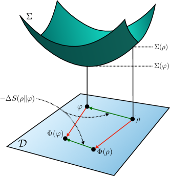
Figure 1: Information-theoretic form of mismatch cost. The top surface represents the entropy production (EP) $\Sigma$ as a function of the initial state $\rho$, for a physical process whose dynamics are described by the quantum channel $\Phi$ (red arrows). The bottom surface represents the set of states $\mathcal{D}$. Eq. 3 says that the extra EP incurred by some initial state $\rho$, additional to the EP incurred by the optimal initial state $\varphi$ which minimizes EP, is equal to the decrease of relative entropy between $\rho$ and $\varphi$ over time (contraction of green arrows).

In this paper, we extend these earlier results in several ways:

• In Section II, we show that the expression for mismatch cost in Eq. 3 holds for arbitrary quantum systems, both finite and infinite dimensional, and coupled to any number of idealized or non-idealized reservoirs. We also show that this expression applies not only when $\varphi$ is the globally optimal initial state, but also when $\varphi$ is the optimal incoherent state (relative to a given set of projection operators), which can be used to decompose mismatch cost into separate quantum and classical contributions. Finally, we derive simple sufficient conditions that guarantee that the optimal initial state $\varphi$ has full support, which allows Eq. 3 to be applied to arbitrary $\rho$ (since Eq. 3 holds only when the support of $\rho$ falls within the support of $\varphi$).

• In Section III, we analyze mismatch cost for the fluctuating EP, that is the trajectory-level EP generated when a physical process undergoes stochastically sampled realizations (campisi2011colloquium, ). We derive an expression for trajectory-level fluctuating mismatch cost, which can be seen as the trajectory-level version of Eq. 3. We also demonstrate that this expression obeys an integral fluctuation theorem.

• In Section IV, we analyze mismatch cost for the instantaneous EP rate incurred at a given instant in time. We show that, similarly to the case of integrated EP and fluctuating EP, mismatch cost for EP rate can be expressed in terms of the instantaneous rate of the contraction of relative entropy between the actual initial state $\rho$ and the optimal initial state $\varphi$ which minimizes the EP rate.

• In Section V, we discuss our results in the context of classical systems. In particular, we demonstrate that all of our results apply to discrete-state and continuous-state classical systems, where they describe the dependence of classical EP on the choice of the initial probability distribution.

After deriving the above results, in Section VI we discuss them within the context of thermodynamics of information processing. In particular, we show that our expressions for mismatch cost imply a fundamental relationship between thermodynamic irreversibility (generation of EP) and logical irreversibility (inability to know the initial state corresponding to a given final state). We use this relationship to derive quantitative bounds on the thermodynamics of quantum error correction, and to propose an operational measure of the logical irreversibility of a quantum channel $\Phi$, which provides a lower bound on the worst-case EP incurred by any physical process that implements $\Phi$.

In Section VII we show that our results for mismatch cost apply not only to EP (which is the main focus of this paper) but in fact to any function that can be written in the general form of Eq. 1, as the increase of system entropy plus some linear term. Examples of such functions include many thermodynamic costs of interest beyond EP, including nonadiabatic EP (horowitz2013entropy, ; horowitz2014equivalent, ; esposito2010three, ; manzanoQuantumFluctuationTheorems2018, ), free energy loss (kolchinsky2017maximizing, ; faist2019thermodynamic, ), and entropy gain (plastino1995fisher, ; holevo2011entropy, ; holevo2011entropyB, ). For any such thermodynamic cost, the extra cost incurred by initial state $\rho$, additional to that incurred by the optimal initial state $\varphi$ which minimizes that cost, is given by the contraction of relative entropy between $\rho$ and $\varphi$ over time.

Before proceeding, we briefly review some relevant prior literature and introduce some necessary notation. We finish with a brief discussion in Section VIII.

I.1 Relevant prior literature

In our own prior work (kolchinsky2016dependence, ; kolchinsky2017maximizing, ; wolpert2020thermodynamic, ), we derived an expression of mismatch cost for the integrated EP incurred by a finite-state classical system. In addition, in this earlier work we showed that mismatch cost has important implications for understanding the thermodynamics of classical information processing, including computation with digital circuits (wolpert2020thermodynamic, ) and deterministic classical Turing machines (kolchinsky2020thermodynamic, ). Finally, we also used mismatch cost to study the thermodynamics of free-energy harvesting systems, both in classical and quantum systems (kolchinsky2017maximizing, ).

Riechers and Gu analyzed mismatch cost for integrated EP incurred by finite-dimensional quantum systems. They used these results to analyze the thermodynamics of information erasure in finite-dimensional quantum systems, as well as the “thermodynamic cost of modularity” (riechers2020initial, ; riechersImpossibilityLandauerBound2021, ).

An important precursor of mismatch cost appeared in (maroney2009generalizing, ). This paper considered one specific quantum process that carries out information processing over a set of classical logical states. It was pointed out that if the protocol is thermodynamically reversible for some initial distribution $\varphi$ over logical states, then for any other initial distribution $\rho$ over the logical states, $\Sigma(\rho)=S({\rho}\|{\varphi})-S(\Phi(\rho)\|\Phi(\varphi))$ (Eq. 168,  maroney2009generalizing, ). This can be seen as a special case of classical mismatch cost, where the optimal state $\varphi$ is thermodynamically reversible (so $\Sigma(\varphi)=0$). A similar result was derived for a specific classical process in (wolpert_arxiv_beyond_bit_erasure_2015, ). Some related ideas were also discussed in Turgut (turgut_relations_2009, ).

I.2 Notational preliminaries

We use $\mathcal{D}$ to indicate the set of all states (i.e., density operators) over the system’s Hilbert space $\mathcal{H}$, which may be finite or infinite dimensional. For any orthogonal set of projection operators $P=\{\Pi_{1},\Pi_{2},\dots\}$, we define

$$\mathcal{D}_{P}:=\{\rho\in\mathcal{D}:\rho=\sum_{\Pi\in P}\Pi\rho\Pi\}$$ (4)

as the set of states that are incoherent relative to projectors in $P$. Note that the set of projection operators $P$ may be complete ($\sum_{\Pi\in P}\Pi=I$) or incomplete ($\sum_{\Pi\in P}\Pi\neq I$). Special cases of $\mathcal{D}_{P}$ include the set of all states $\mathcal{D}$ ($P=\{I\}$), the set of states with support limited to some subspace $\mathcal{H}^{\prime}\subset\mathcal{H}$ ($P=\{\Pi\}$ such that $\Pi\mathcal{H}=\mathcal{H}^{\prime}$), and the set of states diagonal in some orthonormal basis $\{|i\rangle\}_{i}$ ($P=\{|i\rangle\langle i|\}_{i}$). We write

$$\mathcal{H}_{P}=\mathcal{H}\sum_{\Pi\in P}\Pi$$ (5)

to indicate the Hilbert subspace spanned by the projection operators in $P$.

We use the von Neumann entropy of state $\rho\in\mathcal{D}$,

$$S(\rho):=-\mathrm{tr}\{\rho\ln\rho\}.$$

We also use the (quantum) relative entropy, defined for any pair of states $\rho,\varphi\in\mathcal{D}$ as

$$S(\rho\|\varphi):= \begin{cases}\mathrm{tr}\{\rho(\ln\rho-\ln\varphi)\}&\text{if $\mathrm{supp}\,\rho\subseteq\mathrm{supp}\,\varphi$}\\ \infty&\text{otherwise}\end{cases}$$ (6)

For notational convenience, we often write the change of relative entropy under some quantum channel $\Phi$ as

$$\Delta S({\rho}\|{\varphi}) :=S(\Phi(\rho)\|\Phi(\varphi))-S(\rho\|\varphi).$$ (7)

Finally, given some quantum channel $\Phi$ and some reference state $\varphi\in\mathcal{D}$, the Petz recovery map is defined as (Sec. 12.3,  wildeQuantumInformationTheory2017, )

$$\mathcal{R}_{\Phi}^{\varphi}(\rho):=\varphi^{1/2}\Phi^{\dagger}(\Phi(\varphi)^{-1/2}\rho\Phi(\varphi)^{-1/2})\varphi^{1/2}.$$ (8)

The recovery map undoes the effect of $\Phi$ on the reference state, so that $\mathcal{R}_{\Phi}^{\varphi}(\Phi(\varphi))=\varphi$. It can be seen as a generalization of the Bayesian inverse to quantum channels (leiferFormulationQuantumTheory2013, ).

II Mismatch Cost for Integrated EP

In our first set of results, we consider the state dependence of integrated EP, in terms of the additional integrated EP incurred by some initial state $\rho$ rather than the optimal initial state $\varphi$.

Our results apply to $\Sigma(\rho)$ as defined in Eq. 1 in terms of the increase of system entropy plus the entropy flow, where $\Phi$ is some positive and trace-preserving map and the entropy flow $Q$ is some linear function (which we assume is lower-semicontinuous). Our results also apply when $\Sigma(\rho)$ is defined in terms of an explicitly-modeled system+environment that jointly evolve in a unitary manner as $\rho\otimes\omega\to U(\rho\otimes\omega)U^{\dagger}$. In this case, the quantum channel can be expressed in the Stinespring form as $\Phi(\rho)=\mathrm{tr}_{Y}\{U(\rho\otimes\omega)U^{\dagger}\}$ (where $\mathrm{tr}_{Y}$ indicates a partial trace over the environment), and EP can be written as

$$\Sigma(\rho)=S(U(\rho\otimes\omega)U^{\dagger}\|\Phi(\rho)\otimes\omega).$$ (9)

This expression for EP often appears in recent work on quantum thermodynamics (esposito2010entropy, ; ptaszynskiEntropyProductionOpen2019, ; landi2020irreversible, ).

These two formulations of EP, Eq. 1 and Eq. 9, have different advantages and disadvantages. Eq. 1 can be more experimentally accessible since — unlike Eq. 9 – it does not require knowledge of the exact state and evolution of the environment, only the total amount of entropy flow (e.g., as could be measured by a calorimeter). For the same reason, Eq. 1 is also more appropriate for studying EP for a system coupled to “idealized” baths (which have infinite size and instantaneous self-equilibration (breuer2002theory, )). On the other hand, Eq. 9 is more appropriate for studying EP for a system coupled to more realistic “non-idealized” baths (which have finite size and possibly slow relaxation times). From a purely mathematical perspective, the two forms are equivalent for any $\rho$ with finite entropy: Eq. 9 can be rewritten in the form of Eq. 1 and vice versa (see Proposition  in the appendix).

Now consider the set of states $\mathcal{D}_{P}$, defined as in Eq. 4 in terms of a set of projection operators $P$, as well as any state $\rho\in\mathcal{D}_{P}$. As mentioned below, common choices of $\mathcal{D}_{P}$ include the set of all states (corresponding to $P=\{I\}$) and the set of states that are incoherent relative to some basis (corresponding to $P=\{|i\rangle\langle i|\}_{i}$ for some basis $\{|i\rangle\}$). We analyze the mismatch cost of $\rho$, defined as the additional integrated EP incurred by $\rho$ relative to an optimal initial state within $\mathcal{D}_{P}$, $\varphi_{P}\in\mathop{\arg\min}_{\omega\in\mathcal{D}_{P}}\Sigma(\omega)$. Our first result is that as long as $S(\rho\|\varphi_{P})<\infty$, the mismatch cost is equal to the drop in relative entropy between $\rho$ and $\varphi_{P}$ during the process,

$$\Sigma(\rho)-\Sigma(\varphi_{P})=-\Delta S({\rho}\|{\varphi_{P}}).$$ (10)

A sketch of the proof of this result is provided at the end of this section, with details left for Appendix A.

Eq. 10 is a generalization of Eq. 3, which holds for both finite and infinite dimensional systems, as well as for optimizers $\varphi$ within arbitrary sets $\mathcal{D}_{P}$. In the special case when $\mathcal{D}_{P}=\mathcal{D}$ (as induced by $P=\{I\}$), Eq. 10 expresses the “global” mismatch cost, the additional integrated EP incurred by the initial state $\rho$ relative to a global optimizer $\varphi_{\mathcal{D}}\in\mathop{\arg\min}_{\omega\in\mathcal{D}}\Sigma(\omega)$.

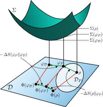
Figure 2: The mismatch cost of $\rho$ relative to the global optimizer $\varphi_{\mathcal{D}}$ can be decomposed into a sum of a “classical” and “quantum” components, Eq. 11. The classical component is given by contraction of relative entropy between $\rho$ and $\varphi_{P}$, the optimal state in the set of states diagonal in the same basis as $\rho$ ($\mathcal{D}_{P}$, shown as a light oval). The quantum component is given by the contraction of relative entropy between $\varphi_{P}$ and $\varphi_{\mathcal{D}}$. (Compare to Fig. 1.)

We can derive various useful decompositions of mismatch cost by applying Eq. 10 in an iterative manner. For example, consider an orthonormal basis $\{|i\rangle\}_{i}$ that diagonalizes $\rho$. Let $P=\{|i\rangle\langle i|\}_{i}$ so that $\mathcal{D}_{P}$ is the set of states diagonal in that basis, which in particular contains $\rho$. Also let $\varphi_{P}\in\mathop{\arg\min}_{\omega\in\mathcal{D}_{P}}\Sigma(\omega)$ be an optimal initial state within $\mathcal{D}_{P}$, and let $\varphi_{\mathcal{D}}\in\mathop{\arg\min}_{\omega\in\mathcal{D}}\Sigma(\omega)$ be a global optimizer. In general, $\varphi_{\mathcal{D}}$ will not be diagonal in the same basis as $\rho$, and so will not belong to $\mathcal{D}_{P}$. We can then write

$$\Sigma(\rho)-\Sigma(\varphi_{\mathcal{D}})=(\Sigma(\rho)-\Sigma(\varphi_{P}))+(\Sigma(\varphi_{P})-\Sigma(\varphi_{\mathcal{D}})),$$

and — assuming that $S(\rho\|\varphi_{P})$ and $S(\varphi_{P}\|\varphi_{\mathcal{D}})$ are finite — apply Eq. 10 to the two terms on the RHS. This leads to the following decomposition of the global mismatch cost of $\rho$ into two non-negative terms, which is visualized in Fig. 2:

$$\Sigma(\rho)-\Sigma(\varphi_{\mathcal{D}})=-\Delta S({\rho}\|{\varphi_{P}})-\Delta S({\varphi_{P}}\|{\varphi_{\mathcal{D}}}).$$ (11)

The first term, $-\Delta S({\rho}\|{\varphi_{P}})$, reflects the mismatch cost between $\rho$ and $\varphi_{P}$. Since these two states are diagonal in the same basis, it can be seen as the classical contribution to mismatch cost. The second term, $-\Delta S({\varphi_{P}}\|{\varphi_{\mathcal{D}}})$, is the purely quantum contribution to mismatch cost, which vanishes when $\rho$ and $\varphi_{\mathcal{D}}$ can be diagonalized in the same basis (since then $\Sigma(\varphi_{P})-\Sigma(\varphi_{\mathcal{D}})=0$).

Note that Eq. 11 is different from the decomposition of mismatch cost into coherent and classical components previously derived in (Eq. 14,  riechers2020initial, ). First, in our decomposition both the classical and quantum are always non-negative (which is not necessarily the case in (riechers2020initial, )). Another difference is that our decomposition does not include terms explicitly related to the “relative entropy of coherence” (baumgratz_quantifying_2014, ), which appear in (Eq. 14,  riechers2020initial, ) (as well as in other classical-vs-quantum decompositions derived for EP in relaxation processes (santos_role_2019, ; francica_role_2019, ) and for quantum work extraction (francica2020quantum, )).

We now state our most generally applicable result for integrated EP mismatch cost. Let $\mathcal{S}\subseteq\mathcal{D}$ be any convex subset of states, which may or may not have the form defined in Eq. 4. Then, for any state $\rho\in\mathcal{S}$ and a minimizer $\varphi_{\mathcal{S}}\in\mathop{\arg\min}_{\omega\in\mathcal{S}}\Sigma(\omega)$, as long as $S(\rho\|\varphi_{\mathcal{S}})<\infty$,

$$\Sigma(\rho)-\Sigma(\varphi_{\mathcal{S}})\geq-\Delta S({\rho}\|{\varphi_{\mathcal{S}}}).$$ (12)

Equality holds if $(1-\lambda)\varphi_{\mathcal{S}}+\lambda\rho\in\mathcal{S}$ for some $\lambda<0$.

Since $\Sigma(\varphi_{\mathcal{S}})\geq 0$ by the second law, Eq. 12 implies

$$\Sigma(\rho)\geq-\Delta S({\rho}\|{\varphi_{\mathcal{S}}}).$$ (13)

The RHS of this bound is non-negative by the monotonicity of relative entropy (muller2017monotonicity, ). Thus, Eq. 13 gives a tighter bound on EP than the second law, $\Sigma(\rho)\geq 0$. This tighter bound reflects the additional EP due to a suboptimal choice of the initial state within any convex set of states $\mathcal{S}\ni\rho$.

We now briefly sketch the derivation of Eqs. 10 and 12, leaving formal proofs for Appendix A. A central idea behind our derivations is that EP is a convex function whose “amount of convexity” has a simple information-theoretic expression. Specifically, using some simple algebra, it can be shown that for any convex mixture $\varphi(\lambda)=(1-\lambda)\varphi+\lambda\rho$ of two states $\rho$ and $\varphi$,

$$(1-\lambda)\Sigma(\varphi)+\lambda\Sigma(\rho)-\Sigma(\varphi(\lambda))=\\ -\lambda\Delta S({\rho}\|{\varphi(\lambda)})-(1-\lambda)\Delta S({\varphi}\|{\varphi(\lambda)}),$$ (14)

The quantity on the right hand side of Eq. 106 has been called entropic disturbance in quantum information theory (shirokovLowerSemicontinuityEntropic2017a, ; buscemiUnifiedApproachInformationDisturbance2009, ; buscemiApproximateReversibilityContext2016, ). It is non-negative by monotonicity of relative entropy (muller2017monotonicity, ), which proves that $\Sigma$ is convex. Next, we consider the directional derivatives of $\Sigma$ at $\varphi$ in the direction of $\rho$,

$${\textstyle{\textstyle\partial_{\lambda}^{+}}}\Sigma(\varphi(\lambda))|_{\lambda=0}=\lim_{{\lambda\to 0^{+}}}\frac{\Sigma(\varphi(\lambda))-\Sigma(\varphi)}{\lambda}.$$

In Proposition  in the appendix, we rearrange Eq. 14 and compute the appropriate limits to show that the directional derivative can be evaluated as

$${\textstyle{\textstyle\partial_{\lambda}^{+}}}\Sigma(\varphi(\lambda))|_{\lambda=0}=\Sigma(\rho)-\Sigma(\varphi)+\Delta S({\rho}\|{\varphi}).$$ (15)

Eq. 12 follows from Eq. 15 and the fact that the directional derivative toward at the minimizer must be non-negative (otherwise one could decrease the value of EP by moving slightly from $\varphi$ to $\rho$, contradicting the fact that $\varphi$ is a minimizer). To derive Eq. 10, suppose that $\varphi$ is a minimizer of EP within a set of states $\mathcal{D}_{P}$ defined as in Eq. 4. If $\rho\geq\alpha\varphi$ for some $\alpha>0$, then the directional derivative in Eq. 15 vanishes (since $\lambda=0$ is the minimizer of the function $\lambda\mapsto\Sigma(\varphi(\lambda))$ in the open set $(-\alpha,1)$), which in combination with Eq. 15 implies Eq. 10. If $\rho\not\geq\alpha\varphi$ for all $\alpha>0$, then Eq. 10 can be derived by considering a sequence of finite-rank projections of $\rho$ onto the top $n$ eigenvectors of $\varphi$, and then using continuity properties of EP and relative entropy.

Note that our expression for mismatch cost, $-\Delta S({\rho}\|{\varphi})$, depends both on the quantum channel $\Phi$ and the optimal state $\varphi\in\mathop{\arg\min}_{\omega}\Sigma(\omega)$. The optimal state $\varphi$ in turn depends on $\Phi$ and the entropy flow function $Q$, which will encode various details of the physical process under consideration (such as the precise trajectory of the driving Hamiltonians, etc.). In general, the same channel $\Phi$ can be implemented with different physical process, which will have different entropy flow functions $Q$ and optimizers $\varphi$. For this reason, different implementations of the same channel $\Phi$ can lead to different values of mismatch cost for the same initial state $\rho$.

We also note that in order to evaluate some of our results numerically, one must find an optimal state $\varphi\in\mathop{\arg\min}_{\omega}\Sigma(\omega)$. In some special cases, $\varphi$ can be found in closed form. One such case is considered below, in our analysis of protocols that obey a symmetry group. Another example occurs when $\varphi\in\mathop{\arg\min}_{\omega\in\mathcal{D}_{P}}$ is a minimizer within some set of states $\mathcal{D}_{P}$ and $\Phi$ is input-independent (there is some $\rho^{\prime}$ such that $\Phi(\rho)=\rho^{\prime}$ for all $\rho$). Then, writing the entropy flow term in trace form as $Q(\rho)=\mathrm{tr}\{\rho A\}$, it is straightforward to show that the minimizer must have the following form :

$$\varphi=e^{-\sum_{\Pi\in P}\Pi A\Pi}/\mathrm{tr}\{e^{-\sum_{\Pi\in P}\Pi A\Pi}\}.$$ (16)

More generally, $\varphi$ can be found using numerical techniques. Because $\Sigma$ is a convex function, this optimization can be performed efficiently (some appropriate algorithms are discussed in (ramakrishnan2019non, )).

II.1 Support conditions

Our result for mismatch cost, Eq. 10, only apply when $S(\rho\|\varphi_{P})<\infty$, for which it is necessary that

$$\mathrm{supp}\,\rho\subseteq\mathrm{supp}\,\varphi_{P}.$$ (17)

(In finite dimensions, Eq. 17 is both necessary and sufficient for $S(\rho\|\varphi_{P})<\infty$; in infinite dimensions, it is necessary but not sufficient). Here, we show that Eq. 17 is satisfied in many cases of interest.

To begin, we consider some set of states $\mathcal{D}_{P}$, while making the weak assumption that the physical process is such that $\Sigma(\rho)$ is finite for all pure states in $\mathcal{D}_{P}$. Then, Proposition  in the appendix shows that the support of the optimizer $\varphi_{P}\in\mathop{\arg\min}_{\omega\in\mathcal{D}_{P}}\Sigma(\rho)$ and its orthogonal complement must be non-interacting subspaces under the action of $\Phi$,

$$\Phi(\varphi_{P})\perp\Phi(\omega)\qquad\forall\omega\in\mathcal{D}_{P}:\omega\perp\varphi.$$ (18)

Now, suppose that $\Phi$ is “irreducible” (over $P$) in the sense that pairs of states which jointly span $\mathcal{H}_{P}$ always incur some overlap,

$$\Phi(\omega)\not\perp\Phi(\omega^{\prime})\quad\forall\omega,\omega^{\prime}\in\mathcal{D}_{P}:\mathrm{supp}\,(\omega+\omega^{\prime})=\mathcal{H}_{P},$$ (19)

where $\mathcal{H}_{P}$ is defined as in Eq. 5. Then, it must be that $\mathrm{supp}\,\varphi_{P}=\mathcal{H}_{P}$, since otherwise there would be some state $\omega\in\mathcal{D}_{P}$ that leads to a contradiction between Eqs. 18 and 19.

To summarize, our results show that if $\Phi$ is irreducible in sense of Eq. 19, then the support condition in Eq. 17 must hold. Note that Eq. 19 is satisfied when the support of all output states is equal,

$$\mathrm{supp}\,\Phi(\rho)=\mathrm{supp}\,\Phi(\omega)\qquad\forall\rho,\omega,$$ (20)

such as the common situation when $\Phi(\rho)>0$ for all $\rho$.

Conversely, if $\Phi$ is not irreducible in the sense of Eq. 19, then one can decompose the $\mathcal{H}_{P}$ into a set of orthogonal subspaces $\mathcal{H}_{1},\mathcal{H}_{2},\dots$ such that Eq. 19 holds in each subspace . Such orthogonal subspaces have been previously called “basins” in the quantum context (riechers2020initial, ) and “islands” in the classical context (wolpert2020thermodynamic, ). Using the arguments above, it can be shown that the optimal state within each basin $\mathcal{H}_{i}$ will have support equal to $\mathcal{H}_{i}$; from Eq. 18, it also follows that optimal states within different basins will not interact under the action of $\Phi$. This resolves a conjecture in (riechers2020initial, ) and justifies the decomposition of $\Sigma$ developed in that paper into a sum of mismatch costs incurred within each basin, plus an “inter-basin coherence” term (for details, see Appendix E in (riechers2020initial, )).

II.2 Example

To illustrate our results with a concrete example, we analyze the EP incurred by a process that obeys a symmetry group. (For related analyses for classical systems see (kolchinsky2020entropy, ), and for quantum systems see (janzing_quantum_2006, ; marvianHowQuantifyCoherence2016, ; vaccaro_tradeoff_2008, )).

To begin, consider a physical process whose dynamics $\Phi$ commute with some unitary $U$,

$$\Phi(U\rho U^{\dagger})=U\Phi(\rho)U^{\dagger}\qquad\forall\rho,$$ (21)

implying that the dynamics are “covariant” under $U$ (holevoNoteCovariantDynamical1993, ) . Furthermore, suppose that the entropy flow function $Q$ associated with the process is invariant under the action of the same unitary,

$$Q(\rho)=Q(U\rho U^{\dagger})\qquad\forall\rho.$$ (22)

Eq. 21 says that in terms of dynamics, it does not matter when one first applies $U$ to the initial $\rho$ and then evolves the system under $\Phi$, or first evolves the system under $\Phi$ and then applies the unitary $U$. Eq. 22 says that in terms of thermodynamics, the entropy flow doesn’t change when one transforms $\rho$ by $U$.

For simplicity, we will first assume that $U$ is some involution ($UU=I$). For concreteness, one can imagine that $U$ involves flipping the state of a qubit in a quantum circuit, which does not interact with the other qubits nor change state during the operation of the circuit (it can be verified that Eq. 21 and Eq. 22 will hold under these assumptions).

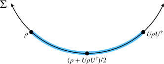
Figure 3: As an example, we consider a physical process in which the EP is invariant under some unitary involution, $\Sigma(\rho)=\Sigma(U\rho U^{\dagger})$ and $UU=I$. For any $\rho$, the uniform mixture $(\rho+U\rho U^{\dagger})/2$ achieves minimum EP within the set of convex combinations of $\rho$ and $U\rho U^{\dagger}$, $\mathcal{S}=\{\lambda\rho+(1-\lambda)U\rho U^{\dagger}:\lambda\in[0,1]\}$ (thick blue line). This leads to the lower bound on EP incurred by state $\rho$, Eq. 25.

Plugging Eq. 21 and Eq. 22 into Eq. 1, and using the fact that von Neumann entropy is invariant under unitary transformations, we see that the EP incurred by the process is invariant under $U$:

$$\Sigma(\rho)=\Sigma(U\rho U^{\dagger})\qquad\forall\rho.$$ (23)

We can now use the results derived above to bound the EP incurred by any initial state $\rho$. To guide intuition, in Fig. 3 we plot the EP incurred by states in the set $\mathcal{S}$ consisting of convex combinations of $\rho$ and $U\rho U^{\dagger}$. Observe that for any such convex combination $\omega=\lambda\rho+(1-\lambda)U\rho U^{\dagger}\in\mathcal{S}$,

$$\Sigma(\omega) =(\Sigma(\omega)+\Sigma(U\omega U^{\dagger}))/2$$

$$\geq\Sigma((\omega+U\omega U^{\dagger})/2)$$

$$=\Sigma((\rho+U\rho U^{\dagger})/2),$$ (24)

where we first used Eq. 23, then the convexity of $\Sigma$, and finally that $(\omega+U\omega U^{\dagger})/2=(\rho+U\rho U^{\dagger})/2$ (which follows from some simple algebra and the fact that $U$ is involution). Eq. 24 implies that minimizer of EP in $\mathcal{S}$ is $(\rho+U\rho U^{\dagger})/2$. Next, for convenience, define the linear operator $\Psi(\rho)=(\rho+U\rho U^{\dagger})/2$. Eq. 13 then gives the following EP bound:

$$\Sigma(\rho) \geq S(\rho\|\Psi(\rho))-S(\Phi(\rho)\|\Phi(\Psi(\rho)))$$

$$=S(\rho\|\Psi(\rho))-S(\Phi(\rho)\|\Psi(\Phi(\rho))),$$ (25)

where in the second line we used that $\Phi$ and $\Psi$ commute (due to linearity of $\Phi$ and Eq. 21).

It is straightforward to generalize this result from simple involutions to more general symmetry groups. Let $G$ be a finite group that acts on $\mathcal{H}$ via a set of unitaries $\{U_{g}:g\in G\}$ (the involution example above corresponds to the $S_{2}$ group which acts on $\mathcal{H}$ via $\{I,U\}$). Suppose that Eq. 21 and Eq. 22 (and hence Eq. 23) hold for each $U_{g}$ individually. Using Eq. 13 and a similar derivation as above, one can show that Eq. 25 still holds, as long as the operator $\Psi$ is defined as a uniform average over all elements of the group, $\Psi(\rho):=\frac{1}{|G|}\sum U_{g}\rho U_{g}^{\dagger}$.

In the quantum information literature, the linear operator $\Psi$ is called a “twirling” operator (vaccaro_tradeoff_2008, ). Moreover, the quantity $S(\rho\|\Psi(\rho))$ in Eq. 25 is known as relative entropy of asymmetry, and it measures the amount of asymmetry in state $\rho$ relative to the group $G$ (marvianHowQuantifyCoherence2016, ; vaccaro_tradeoff_2008, ). Thus, Eq. 25 shows that for any process that is invariant under the action of a symmetry group, in the sense that Eq. 21 and Eq. 22 are obeyed, the EP involved in transforming $\rho\to\Phi(\rho)$ is lower bounded by the decrease of asymmetry during that transformation. Said somewhat differently, any process that obeys a symmetry group must dissipate asymmetry as EP.

III Mismatch Cost for Fluctuating EP

In our second set of results, we analyze EP and mismatch cost at the level of individual stochastic realizations of the physical process. To begin, we briefly review the definitions of fluctuating EP as used in quantum stochastic thermodynamics.

Consider a system that evolves according to the channel $\Phi$ from some initial mixed state $\rho=\sum_{i}p_{i}|i\rangle\langle i|$ to some final mixed state $\Phi(\rho)=\sum_{\phi}p^{\prime}_{\phi}|\phi\rangle\langle\phi|$. Suppose that this stochastic process is carried out multiple times, resulting in a set of randomly sampled realizations. Each realization can be characterized by the associated initial pure state $|i\rangle\langle i|$, the final pure state $|\phi\rangle\langle\phi|$, and the associated entropy flow $q\in\mathbb{R}$ (i.e., the increase of the thermodynamic entropy of the reservoirs that occurs during that realization). The fluctuating EP of realization $(i\!\shortrightarrow\!\phi,q)$ is then given by (esposito2006fluctuation, ; esposito2009nonequilibrium, ; campisi2011colloquium, )

$$\sigma_{\rho}(i\!\shortrightarrow\!\phi,q):=(-\ln p^{\prime}_{\phi}+\ln p_{i})+q,$$ (26)

while the probability of realization $(i\!\shortrightarrow\!\phi,q)$ is given by

$$p_{\rho}(i,\phi,q) =p_{\rho}(i,\phi)p(q|i,\phi)$$ (27)

$$=p_{i}T_{\Phi}(\phi|i)p(q|i,\phi)$$ (28)

$$=p_{i}\mathrm{tr}\{\Phi(|i\rangle\langle i|)|\phi\rangle\langle\phi|\}p(q|i,\phi).$$ (29)

In Eq. 29, $p_{i}$ is the probability of initial pure state $|i\rangle\langle i|$, $p(q|i,\phi)$ is the conditional probability of entropy flow $q$ given the transition $i\!\shortrightarrow\!\phi$, and

$$T_{\Phi}(\phi|i)=\mathrm{tr}\{\Phi(|i\rangle\langle i|)|\phi\rangle\langle\phi|\}$$ (30)

is the conditional probability of the final pure state $|\phi\rangle\langle\phi|$ given the initial pure state $|i\rangle\langle i|$ under $\Phi$.

In quantum stochastic thermodynamics, the terms $q$ and $p(q|i,\phi)$ have been defined and operationalized in various ways, including via two-point projective measurements (esposito2006fluctuation, ; manzanoNonequilibriumPotentialFluctuation2015, ; manzanoQuantumFluctuationTheorems2018, ), weak measurements (allahverdyanNonequilibriumQuantumFluctuations2014a, ), POVMs (kwonFluctuationTheoremsQuantum2019, ), and dynamic Bayesian networks (micadeiQuantumFluctuationTheorems2020, ). In all cases, however, these terms are chosen so that two conditions are satisfied: (1) fluctuating EP agrees with integrated EP in expectation,

$$\langle\sigma_{\rho}\rangle_{p_{\rho}}=\Sigma(\rho),$$ (31)

where $\langle\cdot\rangle_{p_{\rho}}$ indicates expectation under $p_{\rho}(i,\phi,q)$, and (2) fluctuating EP obeys an integral fluctuation theorem (IFT),

$$\langle e^{-\sigma_{\rho}}\rangle_{p_{\rho}}=\gamma,$$ (32)

where $\gamma$ is either equal to 1 or (more generally) some number between 0 and 1 that quantifies the “absolute irreversibility” of the process (funo2015quantum, ). Importantly, our results below do not depend on the particular definition of $q$ and $p(q|i,\phi)$, only on the fact that fluctuating EP can be written in the general form of Eq. 26.

Below, we define fluctuating mismatch cost as the trajectory-level version of the mismatch cost $\Sigma(\rho)-\Sigma(\varphi)$, where $\varphi$ is an optimal initial (mixed) state that minimizes EP. Before proceeding, consider some convex set of states $\mathcal{S}\subseteq\mathcal{D}$. Let $\varphi\in\mathop{\arg\min}_{\omega\in\mathcal{S}}\Sigma(\omega)$ indicate an optimizer in $\mathcal{S}$and let $\rho\in\mathcal{S}$ indicate some state in $\mathcal{S}$ such that $S(\rho\|\varphi)<\infty$. We will assume that

$$\Sigma(\rho)-\Sigma(\varphi)=-\Delta S({\rho}\|{\varphi}).$$ (33)

By Eq. 10, Eq. 33 is satisfied whenever $\mathcal{S}=\mathcal{D}_{P}$; more generally, it is satisfied if the equality form of Eq. 12 holds.

Below we consider two cases differently: (1) the simpler “commuting” case, where the initial state $\rho$ commutes with $\varphi$ and the final state $\Phi(\rho)$ commutes with $\Phi(\varphi)$ (note that this special case includes all classical processes; see Appendix D for details); (2) the more complicated “non-commuting” case, where $\rho$ does not commute with $\varphi$ and/or $\Phi(\rho)$ does not commute with $\Phi(\varphi)$.

III.1 Commuting case

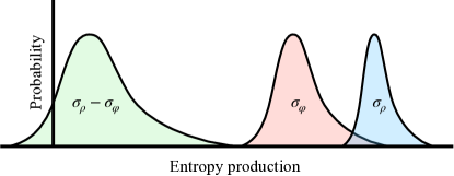
Figure 4: Red and blue curves show the probability distribution of $\sigma_{\rho}$ and $\sigma_{\varphi}$, the fluctuating EP incurred by stochastic realizations sampled from some initial state $\rho$ and the optimal initial state $\varphi$ (which minimizes integrated EP). Each of these fluctuating EP terms individually obeys an integral fluctuating theorem (IFT), Eq. 32. We show that difference of these fluctuating EP terms, $\sigma_{\rho}-\sigma_{\varphi}$, is the fluctuating expression of mismatch cost, and that it also obeys an IFT, Eq. 37.

We first assume that the initial states $\rho$ and $\varphi$ commute, as do the final states $\Phi(\rho)$ and $\Phi(\varphi)$. This means that $\varphi$ can be diagonalized in the same basis as $\rho$, $\varphi=\sum_{i}r_{i}|i\rangle\langle i|$, and $\Phi(\varphi)$ can be diagonalized in the same basis as $\Phi(\rho)$, $\Phi(\varphi)=\sum_{\phi}r^{\prime}_{\phi}|\phi\rangle\langle\phi|$.

We then define the fluctuating mismatch cost of a given realization $(i\!\shortrightarrow\!\phi,q)$ as the difference between $\sigma_{\rho}(i\!\shortrightarrow\!\phi,q)$, the fluctuating EP of the actual realization, and $\sigma_{\varphi}(i\!\shortrightarrow\!\phi,q)$, the fluctuating EP assigned to the same realization $(i\!\shortrightarrow\!\phi,q)$ if the physical process were started from the initial mixed state $\varphi$:

$$\sigma_{\rho}(i\!\shortrightarrow\!\phi,q)-\sigma_{\varphi}(i\!\shortrightarrow\!\phi,q)$$ (34)

$$\qquad=(-\ln p^{\prime}_{\phi}+\ln p_{i})-(-\ln r^{\prime}_{\phi}+\ln r_{i}).$$ (35)

(Note that this is different from $\sigma_{\rho}(i\!\shortrightarrow\!\phi,q)-\Sigma(\varphi)$, the additional fluctuating EP incurred by realization $(i\!\shortrightarrow\!\phi,q)$ under the initial state $\rho$, additional to the expected EP achieved by the optimal initial state $\varphi$.)

We now derive our main results for fluctuating mismatch cost, which are also illustrated in Fig. 4 (see Appendix B for all derivations). First, a simple calculation shows that Eq. 34 is a proper definition of fluctuating mismatch cost, in that its expectation under $p_{\rho}(i,\phi,q)$ is equal to the mismatch cost for integrated EP,

$$\langle\sigma_{\rho}-\sigma_{\varphi}\rangle_{p_{\rho}} =-\Delta S({\rho}\|{\varphi})=\Sigma(\rho)-\Sigma(\varphi).$$ (36)

Second, the fluctuating mismatch cost obeys an IFT,

$$\langle e^{-(\sigma_{\rho}-\sigma_{\varphi})}\rangle_{p_{\rho}}=\gamma\in(0,1],$$ (37)

where $\gamma$ is a “correction factor” that accounts for the fact that some initial pure states are never seen when sampling from $\rho$. Formally, this correction factor is defined as

$$\gamma=\mathrm{tr}\{\Pi^{\rho}(\mathcal{R}_{\Phi}^{\varphi}(\Phi(\rho)))\},$$

where $\mathcal{R}_{\Phi}^{\varphi}$ is the recovery map from Eq. 8 and $\Pi^{\rho}$ is the projection onto the support of $\rho$. This correction factor achieves its maximum value of 1 when the $\rho$ has the same support as $\varphi$, and is closely related to the notion of “absolute irreversibility” studied by Funo et al. (funo2015quantum, ).

Note that mismatch cost for integrated EP is always non-negative, $\Sigma(\rho)-\Sigma(\varphi)\geq 0$, since $\varphi$ is a minimizer of EP. On the other hand, applying Jensen’s inequality to the IFT in Eq. 37 gives the lower bound $\Sigma(\rho)-\Sigma(\varphi)\geq-\ln\gamma$, which is stronger than the first one whenever $\gamma<1$. Furthermore, using standard techniques in stochastic thermodynamics (see Appendix B), the IFT in Eq. 37 implies that negative values of fluctuating mismatch cost are exponentially unlikely,

$$\mathrm{Pr}\big{[}(\sigma_{\rho}-\sigma_{\varphi})\leq-\xi\big{]}\leq\gamma e^{-\xi}.$$ (38)

In stochastic thermodynamics, the fluctuating EP of a trajectory typically reflects how much the trajectory’s probability violates time-reversal symmetry between the process under consideration and a special “time-reversed” version of the process (seifert2012stochastic, ; campisi2011colloquium, ). In contrast, our derivations do not explicitly involve any time-reversed process. However, it is possible to interpret fluctuating mismatch cost as implicitly referencing the violation of time-reversal symmetry. Let $\mathcal{R}_{\Phi}^{\varphi}$ indicate the Petz recovery map, where the optimal initial state $\varphi$ is chosen as the reference state, and let $T_{\mathcal{R}_{\Phi}^{\varphi}}(i|\phi)$ indicate the corresponding conditional probability, defined as in Eq. 30 but for the channel $\mathcal{R}_{\Phi}^{\varphi}$ rather than $\Phi$. Then, as we show in Appendix B, the fluctuating mismatch cost in Eq. 35 can be written as

$$\sigma_{\rho}(i\!\shortrightarrow\!\phi,q)-\sigma_{\varphi}(i\!\shortrightarrow\!\phi,q)=\ln\frac{p_{i}T_{\Phi}(\phi|i)}{p^{\prime}_{\phi}T_{\mathcal{R}_{\Phi}^{\varphi}}(i|\phi)}.$$ (39)

Thus, fluctuating mismatch cost reflects the breaking of time-reversal symmetry, as quantified by the difference between the joint probability of starting on pure state $|i\rangle\langle i|$ and ending on pure state $|\phi\rangle\langle\phi|$ under the regular process, versus the joint probability of starting on pure state $|\phi\rangle\langle\phi|$ and ending on pure state $|i\rangle\langle i|$ under the time-reversed process specified by the Petz recovery map. (See also Ref. (buscemi2020fluctuation, ) for a related fluctuation theorem that also makes use of the Petz recovery map.)

III.2 Non-commuting case

We now consider the more general case when the pair of initial states $\rho,\varphi$ and/or the pair of final states $\Phi(\rho),\Phi(\varphi)$ do not commute. In this case, the pair of initial states $\rho,\varphi$ and/or final states $\Phi(\rho),\Phi(\varphi)$ cannot be simultaneously diagonalized, so one cannot define fluctuating mismatch cost as in Eq. 34. Nonetheless, we show that it is still possible to define a non-commuting version of Eq. 35, which is a proper trajectory-level measure of mismatch cost, obeys an IFT, and reflects the breaking of time-reversal symmetry in a way analogous to Eq. 39.

To derive our results, we employ a framework recently developed by Kwon and Kim (kwonFluctuationTheoremsQuantum2019, ), which provides a fluctuation theorem for quantum processes which is stated in terms of a quantum channel $\Phi$, an initial state $\rho$, and some arbitrary “reference state” $\varphi$. Write the spectral resolutions of the initial mixed states as $\rho=\sum_{i}p_{i}|i\rangle\langle i|$ and $\varphi=\sum_{a}r_{a}|a\rangle\langle a|$, and write the spectral resolutions of the final mixed states as $\Phi(\rho)=\sum_{\phi}p^{\prime}_{\phi}|\phi\rangle\langle\phi|$ and $\Phi(\varphi)=\sum_{\alpha}r^{\prime}_{\alpha}|\alpha\rangle\langle\alpha|$. Then, in the framework of (kwonFluctuationTheoremsQuantum2019, ), each stochastic realization of a process that carries out $\Phi$ on initial state $\rho$ is characterized by four factors: (1) an initial pure state $|i\rangle\langle i|$ in the basis of $\rho$, (2) a final pure state $|\phi\rangle\langle\phi|$ in the basis of $\Phi(\rho)$, (3) an initial (generally off-diagonal) term $|a\rangle\langle b|$ in the basis of the reference state $\varphi$, and (4) a final (generally off-diagonal) term $|\alpha\rangle\langle\beta|$ in the basis of the reference state $\Phi(\varphi)$.

Given these four factors, each realization can be assigned the following fluctuating quantity (Eq. 11,  kwonFluctuationTheoremsQuantum2019, ),

$$m_{\rho,\varphi}(i,a,b\!\shortrightarrow\!\phi,\alpha,\beta)$$ (40)

$$\quad=-\ln p^{\prime}_{\phi}+\ln p_{i}+\frac{1}{2}\ln r^{\prime}_{\alpha}r^{\prime}_{\beta}-\frac{1}{2}\ln r_{a}r_{b}$$ (41)

$$\quad=-\ln p^{\prime}_{\phi}+\ln p_{i}+\ln\frac{T_{\Phi}(\alpha,\beta|a,b)}{T_{\mathcal{R}_{\Phi}^{\varphi}}(a,b|\alpha,\beta)},$$ (42)

where $T_{\Phi}$ and $T_{\mathcal{R}_{\Phi}^{\varphi}}$ encode the forward and backward conditional quasiprobability distributions,

$$T_{\Phi}(\alpha,\beta|a,b) =\langle\alpha|\Phi(|a\rangle\langle b|)|\beta\rangle,$$

$$T_{\mathcal{R}_{\Phi}^{\varphi}}(a,b|\alpha,\beta) =\langle a|\mathcal{R}_{\Phi}^{\varphi}(|\alpha\rangle\langle\beta|)|b\rangle.$$

Note that the backward conditional quasiprobability distribution is defined in terms of the Petz recovery map, Eq. 8. In Ref. (kwonFluctuationTheoremsQuantum2019, ), the quantity $m_{\rho,\varphi}$ is interpreted as a kind of “fluctuating EP” defined relative to an arbitrary reference state $\varphi$, which is purely information-theoretic in nature (i.e., this fluctuating EP does not a priori have anything to do with thermodynamic entropy production). As we discuss below, our interpretation of $m_{\rho,\varphi}$ will be somewhat different.

Before proceeding, we discuss how one might compute the expectation of $m_{\rho,\varphi}$ under a joint probability distribution over realizations $i,a,b\!\shortrightarrow\!\phi,\alpha,\beta$. In fact, no such joint probability distribution can exist, because in general it is impossible to assign valid joint probability to the outcomes of non-commuting observables (allahverdyanExcludingJointProbabilities2018, ). However, one can assign each realization $i,a,b\!\shortrightarrow\!\phi,\alpha,\beta$ the following quasiprobability (Eq. 13,  kwonFluctuationTheoremsQuantum2019, ),

$$\tilde{p}_{\rho}(i,a,b,\phi,\alpha,\beta):=\\ p_{i}\,\langle\phi|\alpha\rangle\langle\alpha|\Phi\big{(}|a\rangle\langle a|i\rangle\langle i|b\rangle\langle b|\big{)}|\beta\rangle\langle\beta|\phi\rangle.$$ (43)

(See Appendix D in (kwonFluctuationTheoremsQuantum2019, ) for details of how the quasiprobability distribution in Eq. 43 can be operationally measured.) Although the quasiprobability distribution $\tilde{p}_{\rho}$ can take negative values for certain outcomes, it nonetheless has positive and correct marginal distributions over the outcomes of the individual observables. Using this, the expectation of $m_{\rho,\varphi}$ (as defined in Eq. 40) under $\tilde{p}_{\rho}$ can be shown to be equal to the contraction of relative entropy between $\rho$ and $\varphi$ (kwonFluctuationTheoremsQuantum2019, , Eq. 25),

$$\langle m_{\rho,\varphi}(i,a,b\!\shortrightarrow\!\phi,\alpha,\beta)\rangle_{\tilde{p}_{\rho}}=-\Delta S({\rho}\|{\varphi}).$$ (44)

Moreover, this quantity also satisfies an IFT (Appendix G in (kwonFluctuationTheoremsQuantum2019, )),

$$\langle e^{m_{\rho,\varphi}(i,a,b\!\shortrightarrow\!\phi,\alpha,\beta)}\rangle_{\tilde{p}_{\rho}}=\gamma,$$ (45)

where $\gamma=\mathrm{tr}\{\Pi^{\rho}(\mathcal{R}_{\Phi}^{\varphi}(\Phi(\rho)))\}\in(0,1]$.

Our interpretation of the quantity $m_{\rho,\varphi}$ is somewhat different from the one discussed in (kwonFluctuationTheoremsQuantum2019, ). As mentioned, we choose the reference state $\varphi$ to be a minimizer of EP, and assume that it satisfies the relation $\Sigma(\rho)-\Sigma(\varphi)=-\Delta S({\rho}\|{\varphi})$, Eq. 33. Then, $m_{\rho,\varphi}$ acquires a concrete thermodynamic meaning: given Eq. 44, it is the expression of fluctuating mismatch cost (i.e., difference of thermodynamic entropy production terms), which applies even when states $\rho$ and $\varphi$ do not commute. This holds because Eq. 44 and Eq. 33 together give the non-commuting analogue of Eq. 36:

$$\langle m_{\rho,\varphi}(i,a,b\!\shortrightarrow\!\phi,\alpha,\beta)\rangle_{\tilde{p}_{\rho}}=\Sigma(\rho)-\Sigma(\varphi).$$ (46)

Similarly, the expression of the breaking of time-reversal symmetry in Eq. 42 is the non-commuting analogue of Eq. 39, while the IFT in Eq. 45 is the non-commuting analogue of Eq. 37.

As mentioned, the quasiprobability distribution $\tilde{p}_{\rho}$ can assign negative values to some joint outcomes. For this reason, one cannot generally derive an exponential bound on the probability of negative mismatch cost as in Eq. 38. Nonetheless, via the series expansion of the exponential function, the IFT in Eq. 45 can still be shown to constrain all moments of fluctuating mismatch cost (kwonFluctuationTheoremsQuantum2019, , p. 13).

Finally, in the case that the pair of initial states $\rho$ and $\varphi$ as well as the pair of final states $\Phi(\rho)$ and $\Phi(\varphi)$ commute — and therefore can be diagonalized in the same basis — the quasiprobability distribution $\tilde{p}_{\rho}$ defined in Eq. 43 reduces to a regular (non-negative) probability distribution,

$$\tilde{p}_{\rho}(i,a,b,\phi,\alpha,\beta)=\begin{cases}p_{\rho}(i,\phi)&\text{if $i\!=\!a\!=\!b$ and $\phi\!=\!\alpha\!=\!\beta$}\\ 0&\text{otherwise}\end{cases}$$

where $p_{\rho}(i,\phi)=p_{i}\mathrm{tr}\{\Phi(|i\rangle\langle i|)|\phi\rangle\langle\phi|\}$ (as appeared in Eq. 27 and Eq. 29). Then, taking expectations under $\tilde{p}_{\rho}(i,a,b,\phi,\alpha,\beta)$ is equivalent to taking expectations under $p_{\rho}(i,\phi)$, which recovers the “commuting case” results (presented in the previous section) as a special case of the more general analysis discussed in this section.

III.3 Example

We now illustrate our results for fluctuating mismatch cost using the example of a “reset” process (see also analyses in (riechers2020initial, ; riechersImpossibilityLandauerBound2021, )).

Consider a finite-dimensional quantum process that maps any initial state $\rho$ to the same final pure state $|\phi\rangle\langle\phi|$, so that the dynamics are described by the following input-independent channel:

$$\Phi(\rho)=|\phi\rangle\langle\phi|\qquad\forall\rho.$$ (47)

This type of process can represent erasure of information (e.g., the reset of a qubit) or the preparation of some special pure state (e.g., preparation of some desired entangled state). Let $\varphi\in\mathop{\arg\min}_{\omega\in\mathcal{D}}\Sigma(\omega)$ indicate the initial mixed state that minimizes EP for this process, and note that we do not assume that $\varphi$ achieves vanishing EP. From Eq. 20 and Section II.1, it is easy to verify that $\varphi$ must have full support.

Now suppose that the process is initialized on some initial mixed state $\rho$. For simplicity, we assume that $\rho$ commutes with $\varphi$, so that both can be diagonalized in the same basis ($\rho=\sum_{i}p_{i}|i\rangle\langle i|$ and $\varphi=\sum_{i}r_{i}|i\rangle\langle i|$). Since we assume a finite-dimensional system and $\varphi$ has full support, $S(\rho\|\varphi)<\infty$ and

$$\Sigma(\rho)-\Sigma(\varphi)=-\Delta S({\rho}\|{\varphi})=S(\rho\|\varphi)$$

by Eq. 10. This means that Eq. 33 holds, allowing us to apply the results we derived for fluctuating mismatch cost in the commuting case, such as Eq. 36 and Eq. 37.

In particular, consider some realization of the process in which the system goes from an initial pure state $|i\rangle\langle i|$ to the final pure state $|\phi\rangle\langle\phi|$. The fluctuating mismatch cost for this realization can be written in the following simple form:

$$\sigma_{\rho}(i\!\shortrightarrow\!\phi,q)-\sigma_{\varphi}(i\!\shortrightarrow\!\phi,q)=\ln p_{i}-\ln r_{i},$$ (48)

where we used Eq. 35 and the fact that $p^{\prime}_{\phi}=r^{\prime}_{\phi}=1$. Eq. 48 means that the fluctuating mismatch cost incurred in mapping $i\!\shortrightarrow\!\phi$ is the log ratio of the probability of pure state $|i\rangle\langle i|$ under the actual initial mixed state $\rho$ and the optimal initial mixed state $\varphi$ that minimizes EP.

Recall that fluctuating mismatch cost obeys the IFT in Eq. 37. Given Eq. 38, this means that the probability of observing negative mismatch is exponentially unlikely: the probability that $\sigma_{\varphi}(i\!\shortrightarrow\!\phi,q)$ exceeds $\sigma_{\rho}(i\!\shortrightarrow\!\phi,q)$ by $\xi$ (or more) is upper bounded by $e^{-\xi}$.

IV Mismatch Cost for EP Rate

In our third set of results, we analyze the state dependence of the instantaneous EP rate. We consider an open quantum system coupled to some number of reservoirs, which evolves according to a Lindblad equation, ${\textstyle\frac{d}{dt}}\rho(t)\!=\!\mathcal{L}(\rho(t))$. The EP rate incurred by state $\rho$ is (spohn1978irreversible, ; spohn_entropy_1978, ; alicki_quantum_1979, )

$$\dot{\Sigma}(\rho)={\textstyle{\textstyle\frac{d}{dt}}}S(\rho(t))+\dot{Q}(\rho),$$ (49)

where $\dot{Q}:\mathcal{D}\to\mathbb{R}$ is a linear function that reflects the rate of entropy flow to the environment. Note that the rate of entropy change ${\textstyle{\textstyle\frac{d}{dt}}}S(\rho(t))$ depends on the Lindbladian $\mathcal{L}$. As above, the precise definition of $\mathcal{L}$ or $\dot{Q}$ will generally reflect various details of the system and the coupled reservoirs. For simplicity, here we assume that $\dim\mathcal{H}<\infty$ (results for the $\dim\mathcal{H}=\infty$ case, which require some additional technicalities, are left for Appendix C).

It is important to note that the derivative in Eq. 49 is evaluated at $t=0$, meaning that $\dot{\Sigma}(\rho)$ expresses the instantaneous EP rate incurred at the same time that the system is found in state $\rho$. An alternative analysis, which we do not consider here, would consider the EP rate incurred at some later time $t>0$, given that the process is initialized in state $\rho$ at $t=0$.

Consider some set of states $\mathcal{D}_{P}$, defined as in Eq. 4 for a set of projection operators $P$. Let $\varphi_{P}\in\mathop{\arg\min}_{\omega\in\mathcal{D}_{P}}\dot{\Sigma}(\omega)$ indicate the state which minimizes the EP rate within this set. Then, for any $\rho\in\mathcal{D}_{P}$ such that $S(\rho\|\varphi_{P})<\infty$, the additional EP rate incurred by $\rho$ above that incurred by $\varphi_{P}$ is given by the instantaneous rate of contraction of the relative entropy between $\rho$ and $\varphi_{P}$,

$$\dot{\Sigma}(\rho)-\dot{\Sigma}(\varphi_{P})=-{\textstyle{\textstyle\frac{d}{dt}}}S(\rho(t)\|\varphi_{P}(t)),$$ (50)

which is the continuous-time analogue of Eq. 10. The proof of this result is sketched at the end of this section, with details left for Appendix C.

We refer to the additional instantaneous EP rate incurred by $\rho$, above that incurred by an optimal state $\varphi_{P}$, the instantaneous mismatch cost of $\rho$. In the special case where $\mathcal{D}_{P}=\mathcal{D}$ (when $P=\{I\}$), Eq. 50 expresses the global instantaneous mismatch cost, reflecting the additional EP rate incurred by state $\rho$ rather than a global optimizer, $\varphi_{\mathcal{D}}\in\mathop{\arg\min}_{\omega\in\mathcal{D}}\dot{\Sigma}(\omega)$.

We can decompose instantaneous mismatch cost by applying Eq. 50 in an iterative manner. In particular, we can derive a decomposition into classical and quantum contributions analogous to Eq. 11. As above, define $P=\{|i\rangle\langle i|\}_{i}$ for an orthonormal basis $\{|i\rangle\}_{i}$ that diagonalizes $\rho$. Then, let $\varphi_{P}\in\mathop{\arg\min}_{\omega\in\mathcal{D}_{P}}\dot{\Sigma}(\omega)$ be an optimal state within $\mathcal{D}_{P}$, and let $\varphi_{\mathcal{D}}\in\mathop{\arg\min}_{\omega\in\mathcal{D}}\dot{\Sigma}(\omega)$ be a global optimizer. Using a similar derivation as in Eq. 11, we can decompose the global instantaneous mismatch cost into two non-negative terms,

$$\dot{\Sigma}(\rho)-\dot{\Sigma}(\varphi_{\mathcal{D}}) =[\dot{\Sigma}(\rho)-\dot{\Sigma}(\varphi_{P})]+[\dot{\Sigma}(\varphi_{P})-\dot{\Sigma}(\varphi_{\mathcal{D}})]$$

$$=-{\textstyle{\textstyle\frac{d}{dt}}}S(\rho(t)\|\varphi_{P}(t))-{\textstyle{\textstyle\frac{d}{dt}}}S(\varphi_{P}(t)\|\varphi_{\mathcal{D}}(t)).$$ (51)

The first term, reflecting the mismatch between $\rho$ and $\varphi_{P}$ which are diagonal in the same basis, is the classical contribution to instantaneous mismatch cost. The second term, reflecting the mismatch between $\varphi_{P}$ and $\varphi_{\mathcal{D}}$, vanishes when $\rho$ and $\varphi_{\mathcal{D}}$ can be diagonalized in the same basis, and is the quantum contribution to instantaneous mismatch cost.

Our most generally applicable result concerns the instantaneous mismatch cost of $\rho$ relative to an optimal state within some arbitrary convex subset of states $\mathcal{S}\subseteq\mathcal{D}$. Given any state $\rho\in\mathcal{S}$ and an optimizer $\varphi_{\mathcal{S}}\in\mathop{\arg\min}_{\omega\in\mathcal{S}}\dot{\Sigma}(\omega)$, as long as $S(\rho\|\varphi_{\mathcal{S}})<\infty$, it is the case that

$$\dot{\Sigma}(\rho)-\dot{\Sigma}(\varphi_{\mathcal{S}})\geq-{\textstyle{\textstyle\frac{d}{dt}}}S(\rho(t)\|\varphi_{\mathcal{S}}(t)),$$ (52)

with equality if $(1-\lambda)\varphi_{\mathcal{S}}+\lambda\rho\in\mathcal{S}$ for some $\lambda<0$. Since $\dot{\Sigma}(\varphi_{\mathcal{S}})\geq 0$ for Lindbladian dynamics (spohn_entropy_1978, ), Eq. 52 implies

$$\dot{\Sigma}(\rho)\geq-{\textstyle{\textstyle\frac{d}{dt}}}S(\rho(t)\|\varphi_{\mathcal{S}}(t)).$$ (53)

The RHS is non-negative by the monotonicity of relative entropy. This provides a tighter bound on the EP rate than the second law, $\dot{\Sigma}(\rho)\geq 0$, which reflects a suboptimal choice of the state within some convex set of states.

We now briefly sketch the proof idea behind Eqs. 50 and 52, leading formal details for Appendix C. First, we use Eq. 49 to define an integrated EP function as $\Sigma(\rho,t)=\int_{0}^{t}\dot{\Sigma}(\rho(t^{\prime}))dt^{\prime}$. Given a pair of states $\rho,\varphi$ with finite EP rate and $S(\rho\|\varphi)<\infty$, we then write the directional derivative of $\dot{\Sigma}$ at $\varphi$ in the direction of $\rho$ as

$${\textstyle\partial_{\lambda}^{+}}\dot{\Sigma}(\varphi(\lambda),t)|_{\lambda=0}:={\textstyle\partial_{\lambda}^{+}}\partial_{t}\Sigma(\varphi(\lambda),t)$$

$$\qquad=\partial_{t}{\textstyle\partial_{\lambda}^{+}}\Sigma(\varphi(\lambda),t)$$

$$\qquad=\partial_{t}[\Sigma(\rho,t)-\Sigma(\varphi,t)+\Delta S({\rho}\|{\varphi})]$$

$$\qquad=\dot{\Sigma}(\rho)-\dot{\Sigma}(\varphi)+{\textstyle{\textstyle\frac{d}{dt}}}S(\rho(t)\|\varphi(t)),$$ (54)

where $\varphi(\lambda)=(1-\lambda)\varphi+\lambda\rho$. In the second line, we used the symmetry of partial derivatives, which (as we prove in the Appendix C) follows from convexity of $\Sigma$. In the third line, we used the expression for the directional derivative of integrated EP, Eq. 15. Eq. 52 follows from Eq. 54, since the directional derivative at a minimizer must be non-negative. To derive Eq. 50, note that if $S(\rho\|\varphi)<\infty$, then $\mathrm{supp}\,\rho\subseteq\mathrm{supp}\,\varphi$ and so it is possible to move from $\varphi\in\mathcal{D}_{P}$ both toward and away from $\rho\in\mathcal{D}_{P}$ while remaining within the set $\mathcal{D}_{P}$. Since $\varphi$ is a minimizer of the EP rate within $\mathcal{D}_{P}$, this means that the directional derivative ${\textstyle\partial_{\lambda}^{+}}\dot{\Sigma}(\varphi(\lambda),t)|_{\lambda=0}$ must vanish.

IV.1 Support conditions

Our result for mismatch cost, Eq. 50, only applies when $S(\rho\|\varphi_{P})<\infty$. This condition in turn requires that

$$\mathrm{supp}\,\rho\subseteq\mathrm{supp}\,\varphi_{P}.$$ (55)

Here, we show that Eq. 55 is satisfied in many cases of interest.

In Proposition  in the appendix, we prove that Eq. 55 holds for all $\rho\in\mathcal{D}_{P}$ and $\varphi_{P}\in\mathop{\arg\min}_{\omega\in\mathcal{D}_{P}}\dot{\Sigma}(\omega)$ as long as the Lindbladian $\mathcal{L}$ satisfies the following “irreducibility” condition:

$$\mathrm{supp}\,\mathcal{L}(\rho)\not\subseteq\mathrm{supp}\,\rho\quad\forall\rho\in\mathcal{D}_{P}:\mathrm{supp}\,\rho\neq\mathcal{H}_{P},$$ (56)

where $\mathcal{H}_{P}$ is defined as in Eq. 5 (we also assume that $\dim\mathcal{H}<\infty$). Eq. 56 says that whenever some state $\rho$ with partial support evolves under $\mathcal{L}$, some probability “leaks out” of subspace spanned by $\rho$. In the terminology of (baumgartnerAnalysisQuantumSemigroups2008a, ; baumgartnerAnalysisQuantumSemigroups2008, ), Eq. 56 means that $\mathcal{L}$ does not have any non-trivial “lazy subspaces”.

If $\mathcal{L}$ is not irreducible in the sense of Eq. 56, it may be possible to decompose the overall Hilbert space into a set of irreducible subspaces such that Eq. 133 holds in each one (baumgartnerAnalysisQuantumSemigroups2008a, ; baumgartnerAnalysisQuantumSemigroups2008, ). Such subspaces have been called enclosures in the literature (see (carboneIrreducibleDecompositionsStationary2016, ) for details) and are the continuous-time analogue of “basins” discussed above. We leave analysis of instantaneous mismatch cost with multiple enclosures for future work.

IV.2 Example

We briefly illustrate our results for instantaneous mismatch cost by deriving a novel bound on the EP rate incurred in a non-equilibrium stationary state.

Consider a finite-dimensional system that evolves in continuous time according to some Lindbladian $\mathcal{L}$. Assume that the system is coupled to multiple reservoirs and has an associated non-equilibrium stationary state $\pi$. In addition, let $\varphi\in\mathop{\arg\min}_{\omega\in\mathcal{D}}\dot{\Sigma}(\omega)$ be a state that achieves the minimal EP rate. Eq. 53 then implies the following bound on the stationary EP rate,

$$\dot{\Sigma}(\pi) \geq-{\textstyle{\textstyle\frac{d}{dt}}}S(\pi(t)\|\varphi(t))=-{\textstyle\frac{d}{dt}}S(\pi\|\varphi(t)),$$ (57)

where ${\textstyle\frac{d}{dt}}\pi(t)=\mathcal{L}(\pi)=0$ by assumption of stationarity.

Eq. 57 shows that for any continuous-time process, the stationary EP rate is lower bounded by the rate at which the minimally dissipative state $\varphi$ approaches the stationary state $\pi$ in relative entropy.

V Mismatch Cost in Classical Systems

We now discuss mismatch cost in the context of classical systems. We consider both discrete-state classical systems (as might be derived by coarse-graining an underlying phase space (talknerRateDescriptionFokkerPlanck2004, )) and continuous-state classical systems. For more details, see Appendix D.

V.1 Classical integrated EP

We begin by overviewing the definition of integrated EP in classical systems.

Consider a classical system with state space $X$ which undergoes a driving protocol over time interval $t\in[0,\tau]$, while coupled to some thermodynamic reservoirs. We use the notation $p^{\prime}$ to indicate the final probability distribution at time $t=\tau$ corresponding to the initial probability distribution $p$ at time $t=0$. (Note that we use the term “probability distribution” to indicate a probability mass function for discrete-state systems and a probability density function for continuous-state systems.) In addition, following classical stochastic thermodynamics (van2013stochastic, ; seifert2012stochastic, ), we use $\mathrm{P}(\bm{x}|x_{0})$ to indicate the conditional probability of the system undergoing the trajectory $\bm{x}=\{x_{t}:t\in[0,\tau]\}$ under the regular (“forward”) protocol given initial microstate $x_{0}$. Sometimes we will also consider the conditional probability $\tilde{\mathrm{P}}(\tilde{\bm{x}}|\tilde{x}_{\tau})$ of observing the time-reversed trajectory $\tilde{\bm{x}}=\{\tilde{x}_{\tau-t}:t\in[0,\tau]\}$ under the time-reversed driving protocol given initial microstate $\tilde{x}_{\tau}$ (tilde notation like $\tilde{x}$ indicates conjugation of odd variables such as momentum (ford_entropy_2012, ; spinneyNonequilibriumThermodynamicsStochastic2012, )).

For classical systems, there are several ways of defining integrated EP as a function of the initial probability distribution. The first way is the classical analogue of Eq. 1,

$$\mathsf{\Sigma}(p)=\mathsf{S}(p^{\prime})-\mathsf{S}(p)+G(p),$$ (58)

where $\mathsf{\Sigma}(\cdot)$ indicates classical EP as a function of the initial probability distribution, $\mathsf{S}(\cdot)$ indicates classical Shannon entropy and $G(\cdot)$ is a linear function that reflects the entropy flow to the environment. As above, the precise definition of the entropy flow term will depend on the physical setup, such as the number and type of coupled reservoirs.

A second way to define integrated EP in classical systems is in terms of the relative entropy between the trajectory probability distribution under the forward process and the time-reversed backward process (spinneyEntropyProductionFull2012, ; esposito_three_2010, ),

$$\mathsf{\Sigma}(p)=D\big{(}\mathrm{P}(\bm{X}|X_{0})p(X_{0})\|\tilde{\mathrm{P}}(\tilde{\bm{X}}|\tilde{X}_{\tau})p^{\prime}(X_{\tau})\big{)},$$ (59)

where $D(\cdot\|\cdot)$ indicates the classical relative entropy (also called the Kullback-Leibler divergence). Eq. 59 expresses integrated EP directly in terms of the “time-asymmetry” of the stochastic process (parrondoEntropyProductionArrow2009a, ). Note that the expression in Eq. 59 is a special case of the expression in Eq. 58, since it can be put in the form of the latter by defining the entropy flow in Eq. 58 as the expectation $G(p)=\Big{\langle}\ln\mathrm{P}(\bm{x}|x_{0})-\ln\tilde{\mathrm{P}}(\tilde{\bm{x}}|\tilde{x}_{\tau})\Big{\rangle}_{\mathrm{P}(\bm{x}|x_{0})p(x_{0})}$, and then performing some simple rearrangement.

There is also a third way to define integrated EP for continuous-state classical systems in phase space. Consider some system $X$, and let $Y$ indicate its explicitly modeled environment (typically, $Y$ will indicate the state of one or more heat baths). Assume that $X$ and $Y$ jointly evolve in a Hamiltonian manner starting from an initial distribution $p(x_{0},y_{0})=p(x_{0})\pi(y_{0}|x_{0})$ at time $t=0$ to some final distribution $p^{\prime}(x_{\tau},y_{\tau})$ at time $t=\tau$, where $\pi(y_{0}|x_{0})$ is the conditional equilibrium distribution induced by some system-environment Hamiltonian. The integrated EP incurred by initial distribution $p$ can then be defined as

$$\mathsf{\Sigma}(p)=D({p^{\prime}(X_{\tau},Y_{\tau})}\|{p^{\prime}(X_{\tau})\pi({Y_{\tau}|X_{\tau}})}).$$ (60)

(see (Eq. 15,  millerEntropyProductionTime2017, ), (Eq. 49,  strasberg_stochastic_2017, ), and (seifertFirstSecondLaw2016a, )). Eq. 60 is the classical analogue of Eq. 9, though generalized to allow equilibrium correlations between the environment and the system (see discussion in Appendix A of (strasberg_stochastic_2017, )).

We now discuss mismatch cost for classical integrated EP. First, consider a discrete-state classical system, such that the state space $X$ is a countable set. In this case, our results for quantum mismatch cost can be directly applied, since a discrete-state classical process can be expressed as a special case of a quantum process. In particular, let $\mathcal{D}_{P}$, defined as in Eq. 4, indicate the set of density operators diagonal in some fixed reference basis. Then, any probability distribution $p$ over $X$ can be expressed as a density operator in $\mathcal{D}_{P}$, and any classical dynamics can be expressed as a special quantum channel that maps elements of $\mathcal{D}_{P}$ to elements of $\mathcal{D}_{P}$ (see Section D.1 for details). Under this mapping, the expressions for quantum and classical EP (Eq. 1 versus Eqs. 58, 59 and 60) become equivalent, and we can analyze mismatch cost for classical integrated EP using the results presented above, such as Eqs. 10 and 12. For instance, we have the following classical analogue of Eq. 10: given any initial distribution $p$ and an optimal initial distribution within the set of all distributions, $r\in\mathop{\arg\min}_{s}\mathsf{\Sigma}(s)$, mismatch cost can be written as

$$\mathsf{\Sigma}(p)-\mathsf{\Sigma}(r)=-\Delta D(p\|r),$$ (61)

as long as $D(p\|r)<\infty$.

For classical systems in continuous state space, such that $X\subseteq\mathbb{R}^{n}$, the mapping from our quantum results to classical mismatch cost is not as direct, because in general it is not possible to represent a continuous probability distribution in terms of a density operator over a separable Hilbert space. Nonetheless, as long as an appropriate “translation” is carried out, the same proof techniques used to derive mismatch cost results for quantum integrated EP can also be used to derive analogous results for continuous classical systems, such as Eq. 61. This translation is described in detail in Section D.2.

V.2 Classical fluctuating EP

Next, we show that our results for fluctuating mismatch cost also apply to classical systems. The underlying logic of the derivation is the same as for the commuting case for quantum systems described in Section III.1, though with somewhat different notation.

Consider a classical system that undergoes a physical process, which starts from the initial distribution $p$ and ends on the final distribution $p^{\prime}$. In general, the fluctuating EP incurred by some state trajectory $\bm{x}$ can be expressed as (seifert2012stochastic, )

$$\sigma_{p}(\bm{x})=\ln p(x_{0})-\ln p^{\prime}(x_{\tau})+q(\bm{x}),$$

where $q(\bm{x})$ is the increase of the entropy of all coupled reservoirs incurred by trajectory $\bm{x}(t)$. Let $r$ indicate the initial probability distribution that minimizes EP, so that Eq. 61 holds, and let $r^{\prime}$ indicate the corresponding final distribution. We define classical fluctuating mismatch cost as the difference between the fluctuating EP incurred by the trajectory $\bm{x}$ under the actual initial distribution $p$ and the optimal initial distribution $r$,

$$\sigma_{p}(\bm{x})-\sigma_{r}(\bm{x})=\\ {}[-\ln p^{\prime}(x_{\tau})+\ln p(x_{0})]-[-\ln r^{\prime}(x_{\tau})+\ln r(x_{0}))],$$ (62)

which is the classical analogue of Eq. 34. It is easy to verify that Eq. 62 is the proper trajectory-level expression of classical mismatch cost,

$$\langle\sigma_{p}-\sigma_{r}\rangle_{\mathrm{P}(\bm{x}|x_{0})p(x_{0})}=-\Delta D(p\|r)=\mathsf{\Sigma}(p)-\mathsf{\Sigma}(r).$$ (63)

Moreover, using a derivation similar to the one in Appendix B, it can be shown that Eq. 62 obeys an IFT,

$$\langle e^{-(\sigma_{p}-\sigma_{r})}\rangle_{\mathrm{P}(\bm{x}|x_{0})p(x_{0})}=\gamma,$$ (64)

where $\gamma\in(0,1]$ is a correction factor that equals 1 when $p$ and $r$ have the same support (see Eq. 148 in the appendix). Eq. 63 and Eq. 64 are the classical analogues of Eq. 36 and Eq. 37 respectively. Moreover, the IFT in Eq. 64 implies that same exponential bound on negative mismatch cost as in Eq. 38.

We can also derive the classical analogue of Eq. 39, which expresses fluctuating mismatch cost in terms of the breaking of time-reversal symmetry. Note that for a classical system, the Petz recovery map is simply the Bayesian inverse of the conditional probability distribution $\mathrm{P}(x_{\tau}|x_{0})$ with respect to the probability distribution $r$, $\mathrm{P}(x_{0}|x_{\tau})=\mathrm{P}(x_{\tau}|x_{0})r(x_{0})/r^{\prime}(x_{\tau})$ (leiferFormulationQuantumTheory2013, ; wildeQuantumInformationTheory2017, ). In Appendix D, we show that

$$\sigma_{p}(\bm{x})-\sigma_{r}(\bm{x}) =\ln\frac{\mathrm{P}(x_{\tau}|x_{0})p(x_{0})}{\mathrm{P}(x_{0}|x_{\tau})p^{\prime}(x_{\tau})},$$ (65)

Thus, the fluctuating mismatch cost for a classical system quantifies the time-asymmetry between the forward process and the reverse process, as defined by the Bayesian inverse of the forward process run on the optimal initial distribution $r$.

For more detailed derivations, see Section D.1.2 for discrete-state classical systems, and Section D.2.2 for continuous-state classical systems.

V.3 Classical EP rate

Finally, we discuss instantaneous mismatch cost in the context of classical systems.

Consider a classical system whose probability distribution at time $t=0$ evolves according to a master equation,

$${\textstyle\frac{d}{dt}}p(t)=Lp(t),$$

where $L$ is a linear operator that is the infinitesimal generator of the dynamics. For a discrete-state classical system, $L$ will be a rate matrix specifying transitions rates between different states, while for a continuous-state classical system, $L$ will typically be a Fokker-Planck operator. The classical EP rate can be written as (esposito2010three, )

$$\dot{\mathsf{\Sigma}}(p)={\textstyle\frac{d}{dt}}\mathsf{S}(p(t))+\dot{G}(p),$$ (66)

where $\dot{G}(p)$ is the rate of entropy flow to environment. As always, the form of $\dot{G}(p)$ will depend on the specifics of the physical process, but can generally be expressed as an expectation of some function over the microstates. Eq. 66 is the classical analogue of Eq. 49.

A discrete-state classical system can be formulated as a special case of a quantum system, as mentioned above in Section V.1 and described in more detail in Appendix D. In particular, one can always express a discrete classical distribution as a density matrix and a discrete rate matrix as a specially-constructed Lindbladian. Under this mapping, the expressions for quantum and classical EP rate (Eq. 49 versus Eq. 66) become equivalent, and we can analyze instantaneous mismatch cost for discrete-state classical systems using the results presented above for quantum systems, such as Eq. 50, Eq. 52, and Eq. 53. In particular, we have the following classical analogue of Eq. 50: given any distribution $p$ and an optimal distribution $r\in\mathop{\arg\min}_{s}\dot{\mathsf{\Sigma}}(s)$ which minimizes EP rate,

$$\dot{\mathsf{\Sigma}}(p)-\dot{\mathsf{\Sigma}}(r)=-{\textstyle\frac{d}{dt}}D(p(t)\|r(t)),$$ (67)

as long as $D(p\|r)<\infty$.

As mentioned above, for continuous-state classical systems, the mapping to the quantum formalism is not as direct. Nonetheless, the same proof techniques used to derive instantaneous mismatch cost for quantum systems can be used to derive analogous results for continuous classical systems, such as Eq. 67. This can be done as long as an appropriate “translation” is carried out between classical and quantum formulations, which is described in detail in Section D.2.3.

VI Logical vs. Thermodynamic Irreversibility

The relationship between thermodynamic irreversibility (generation of EP) and logical irreversibility (inability to know the initial state corresponding to a given final state) is one of the foundational issues in the thermodynamics of computation (bennettNotesHistoryReversible1988, ). Despite some confusion in the early literature, it is now well-understood that logically irreversible operations can in principle be carried out in a thermodynamically reversible manner, without generating any EP (maroney_absence_2005, ; sagawa2014thermodynamic, ; wolpert2019stochastic, ).

At the same time, our results demonstrate a different kind of universal relationship between logical and thermodynamic irreversibility. By Eq. 12, the mismatch cost of $\rho$ is lower-bounded by the contraction of relative entropy $-\Delta S({\rho}\|{\varphi})$, which is a principled information-theoretic measure of the logical irreversibility of the quantum channel $\Phi$ on the pair of states $\rho,\varphi$. This measure reaches its maximal value of $S(\rho\|\varphi)$ if and only if $\Phi(\varphi)=\Phi(\rho)$, in which case all information about the choice of initial state ($\rho$ vs. $\varphi$) is lost. It reaches its minimal value of 0 if and only if the map $\Phi$ is logically reversible on the pair of states $\rho,\varphi$, meaning that the Petz recovery map $\mathcal{R}_{\Phi}^{\varphi}$ can perfectly restore both initial states $\rho$ and $\varphi$ from the output of $\Phi$, $\mathcal{R}_{\Phi}^{\varphi}(\Phi(\varphi))=\varphi$ and $\mathcal{R}_{\Phi}^{\varphi}(\Phi(\rho))=\rho$ (petz1988sufficiency, ; mosonyi2004structure, ; wildeRecoverabilityQuantumInformation2015a, ). For a unitary channel, $-\Delta S({\rho}\|{\varphi})=0$ for all pairs of states $\rho,\varphi$.

Now imagine a physical process that implements some map $\Phi$ and achieves minimal EP on some initial state $\varphi$. Our results imply that the thermodynamic cost associated with choosing suboptimal initial states, in terms of the additional EP that is generated on those initial states above the minimum possible, increases with degree of logical irreversibility of the channel $\Phi$. This is consistent with the fact that the minimal EP incurred by a given process that implements $\Phi$, $\min_{\omega}\Sigma(\omega)$, does not directly depend on the logical irreversibility of $\Phi$ (and can vanish even for logically irreversible channels).

Interestingly, recent work has uncovered the following inequality between the contraction of relative entropy and the accuracy of “recovery maps” (jungeUniversalRecoveryMaps2018, ),

$$-\Delta S({\rho}\|{\varphi})\geq-2\ln F(\rho,\mathcal{N}_{\Phi}^{\varphi}(\Phi(\rho))),$$ (68)

where $F(\cdot,\cdot)$ is fidelity and $\mathcal{N}_{\Phi}^{\varphi}$ is a recovery map closely related to Eq. 8. This inequality provides an information-theoretic condition for high-fidelity recovery of an initial state $\rho$ that undergoes a noisy operation $\Phi$, which is of fundamental interest in quantum error correction. Now consider a process that implements the map $\Phi$ and achieves minimal EP on the initial state $\varphi$. Combining Eqs. 10 and 68 along with $\Sigma(\varphi)\geq 0$ gives the inequality

$$F(\rho,\mathcal{N}_{\Phi}^{\varphi}(\Phi(\rho))\geq e^{-\Sigma(\rho)/2},$$

which implies that high-fidelity recovery of $\rho$ by $\mathcal{N}_{\Phi}^{\varphi}$ is possible only if the process incurs a small amount of EP on the initial state $\rho$. Conversely, if $\mathcal{N}_{\Phi}^{\varphi}$ performs poorly at recovering $\rho$, then the EP incurred by initial state $\rho$ must be large. While this relationship between the fidelity of recovery and EP has been discussed for simple relaxation processes to equilibrium (alhambraWorkReversibilityQuantum2018a, ), our results show that it actually holds for a much broader set of processes, including ones with arbitrary driving and possibly coupled to multiple reservoirs.

Motivated by these results, and in the spirit of recent work on information-theoretic characterization of quantum channels (faist2019thermodynamic, ; gourHowQuantifyDynamical2019, ; gourEntropyQuantumChannel2020, ), we propose the following measure of the logical irreversibility of a given map $\Phi$:

$$\Lambda(\Phi):=\inf_{\varphi\in\mathcal{D}}\sup_{\rho\in\mathcal{D}}-\Delta S({\rho}\|{\varphi}).$$ (69)

Our measure has a simple operational interpretation in thermodynamic terms: for any physical process that implements $\Phi$, there must be some initial state that incurs EP of at least $\Lambda(\Phi)$, as follows from Eq. 10 and $\Sigma(\varphi)\geq 0$. $\Lambda(\Phi)$ can be related to some existing measures of logical irreversibility, such as the “contraction coefficient of relative entropy” from quantum information theory (choi_equivalence_1994, ; raginsky2002strictly, ; hiai2016contraction, ), $\eta(\Phi)=\sup_{\rho\neq\omega}S(\Phi(\rho)\|\Phi(\omega))/S(\rho\|\omega)$. Some simple algebra shows that $\Lambda(\Phi)\geq(1-\eta(\Phi))\ln d$, where $d$ the dimension of the Hilbert space. More generally, it is easy to verify that $\Lambda(\Phi)$ achieves its minimum value of 0 if $\Phi$ is unitary, and achieves its maximum value of $\ln d$ if $\Phi$ is input-independent (where $d$ the dimension of the Hilbert space).

Some care should be taken in relating these results to earlier arguments concerning “reversible computation”. Suppose that one wishes to implement some logically irreversible map $\Phi$ while minimizing EP. Our results show that it is possible to completely eliminate the mismatch cost of running $\Phi$ by “embedding” $\Phi$ within some larger logically reversible (i.e., unitary) map $\Phi^{\prime}$, since $\Lambda(\Phi^{\prime})=0$. This is related to the idea of using logically reversible embeddings to reduce the minimal generated heat involved in carrying out a logically irreversible computation (bennett1973logical, ; bennettNotesHistoryReversible1988, ; fredkin1982conservative, ; bennett1989time, ; levine1990note, ; lange2000reversible, ).

At the same time, this strategy incurs an additional “storage cost” of having to encode extra output information in physical degrees of freedom (bennett1973logical, ). This additional cost, which would not exist in a direct (i.e., logically irreversible) implementation of $\Phi$, can itself be interpreted thermodynamically, since it involves an increase of the entropy of those extra physical degrees of freedom (for further discussion of related issues, see (Sec. 11,  wolpert2019stochastic, )). Thus, when considering implementing a desired channel $\Phi$ via some larger embedding $\Phi^{\prime}$, there is a tradeoff between mismatch cost (which decreases as the logical reversibility of $\Phi^{\prime}$ increases) and storage cost (which increases as the logical reversibility of $\Phi^{\prime}$ increases).

Of course, one can avoid the storage cost by first carrying out the larger embedding $\Phi^{\prime}$ and then erasing the additional output information with an erasure map $\Phi^{\prime\prime}$, so that the combined map recovers the original logically irreversible map, $\Phi=\Phi^{\prime\prime}\circ\Phi^{\prime}$. In this case, however, the combined operation has mismatch cost of $S(\rho\|\varphi)-S(\Phi(\rho)\|\Phi(\varphi))$ on initial state $\rho$, where $\varphi$ is the initial state that minimizes EP for this combined operation. For any given $\rho$, this mismatch cost may be larger or smaller than the mismatch cost incurred by some other implementation of $\Phi$ (such as an implementation that does not make use of logically reversible intermediate steps), depending on the optimal initial state of that other implementation (see also related discussion in Section II).

VI.1 Example

Consider a qubit which undergoes an input-independent reset process, so that all input states $\rho$ are mapped to the output pure state $|0\rangle\langle 0|$,

$$\Phi(\rho)=|0\rangle\langle 0|\quad\forall\rho.$$

(See also Section III.3.) For this process,

$$\Lambda(\Phi) :=\inf_{\varphi\in\mathcal{D}}\sup_{\rho\in\mathcal{D}}-\Delta S({\rho}\|{\varphi})$$

$$=\inf_{\varphi\in\mathcal{D}}\sup_{\rho\in\mathcal{D}}S(\rho\|\varphi)$$ (70)

It is easy to verify that this optimization problem is solved by taking $\varphi$ to be the maximally mixed state, $\varphi=(|0\rangle\langle 0|+|1\rangle\langle 1|)/2$, and taking $\rho$ to be any pure state , which gives

$$\Lambda(\Phi)=\ln 2.$$

Thus, for any physical implementation of a qubit reset, there must exist initial states $\rho$ which have $\Sigma(\rho)\geq\ln 2$.

VII Mismatch Cost Beyond EP

This paper was formulated in terms of the state dependence of entropy production. However, our results also apply to many other important “cost functions” that appear in nonequilibrium thermodynamics and quantum information theory. In particular, as we show in Appendix A and Appendix D, our results for mismatch costs hold not only for EP, but for any “EP-type” function $C(\rho)$ that can be written in the following general form:

$$C(\rho)=S(\Phi(\rho))-S(\rho)+F(\rho),$$ (71)

where $\Phi$ is any quantum channel (which may have different input and output Hilbert spaces) and $F$ is any linear functional. Our expression of EP, Eq. 1, is a special case of Eq. 71, which arises when $F$ is defined as the entropy flow $Q$. (There is also an analogous generalization of EP as alternatively defined in Eq. 9; see the appendix for details).

There are many costs beyond EP can be expressed in the form of Eq. 71, including:

1. Nonadiabatic EP, the contribution to EP arising from the system being out of stationarity. For a Markovian system evolving over $t\in[0,\tau]$, nonadiabatic EP can be written as (horowitz2013entropy, ; horowitz2014equivalent, ; esposito2010three, ; manzanoQuantumFluctuationTheorems2018, ),

   $$C(\rho)=S(\Phi(\rho))-S(\rho)-\int_{0}^{\tau}\mathrm{tr}\{(\partial_{t}\Phi_{t}(\rho))\ln\rho_{t}^{\text{st}}\}\,dt,$$

   where $\Phi_{t}(\rho)$ is the system’s state at time $t$ given initial state $\rho$ (and $\Phi(\rho)=\Phi_{\tau}(\rho)$) and $\rho_{t}^{\text{st}}$ is the nonequilibrium stationary state at time $t$. With some rearranging, nonadiabatic EP for non-Markovian evolution (garcia2012nonadiabatic, ) and for quantum processes with measurement (manzanoNonequilibriumPotentialFluctuation2015, ; manzanoQuantumFluctuationTheorems2018, ) can also be put into the form of Eq. 71.

2. The free energy loss (kolchinsky2017maximizing, ; faist2019thermodynamic, ; navascues2015nonthermal, ; muller2018correlating, ),

   $$C(\rho) =\beta[\mathcal{F}_{\beta}(\rho,H_{0})-\mathcal{F}_{\beta}(\Phi(\rho),H_{\tau})]$$

   $$=S(\Phi(\rho))-S(\rho)+\beta\mathrm{tr}\{\rho(H_{0}-\Phi^{\dagger}(H_{\tau}))\},$$ (72)

   where $\mathcal{F}_{\beta}(\rho,H)=\mathrm{tr}\{\rho H\}-\beta^{-1}S(\rho)$ is the nonequilibrium free energy at inverse temperature $\beta$, and $H_{0}$ and $H_{\tau}$ are the initial and final Hamiltonians. Note that Eq. 72 can be negative, in which case it reflects a net gain of free energy (from this point of view, the optimal initial state that minimizes Eq. 72 can also be seen as the state that maximizes harvesting of free energy (kolchinsky2017maximizing, )). When $H_{0}=H_{\tau}$, the minimum value of Eq. 72 across all initial states, as would be achieved by an optimizer $\varphi$, is sometimes called the “thermodynamic capacity” of $\Phi$, and provides operational bounds on quantum work extraction (navascues2015nonthermal, ; faist2019thermodynamic, ).

3. The drop of availability, which is also called extractable work (schlogl1985thermodynamic, ; deffnerNonequilibriumEntropyProduction2011a, ; kolchinsky2017maximizing, ; esposito2011second, ),

   $$C(\rho) =S(\rho\|\pi_{0})-S(\Phi(\rho)\|\pi_{\tau})$$

   $$=S(\Phi(\rho))-S(\rho)+\mathrm{tr}\{\rho[\Phi^{\dagger}(\ln\pi_{\tau})-\ln\pi_{0}]\}$$ (73)

   where $\pi_{t}=e^{-\beta H_{t}}/Z$ is the Gibbs state at time $t$. Note that the difference between Eq. 73 and Eq. 72 is $\beta$ times the decrease of equilibrium free energy, which is a constant that doesn’t depend on $\rho$ and vanishes when $H_{0}=H_{\tau}$.

4. The entropy gain of a given channel and initial state (holevo2011entropy, ; ramakrishnan2019non, ; holevo2011entropyB, ; buscemiApproximateReversibilityContext2016, ; das2018fundamental, ; alicki2004isotropic, ),

   $$C(\rho)=S(\Phi(\rho))-S(\rho).$$ (74)

   The minimum entropy gain for a given channel has been considered when analyzing the capacity of quantum channels (alicki2004isotropic, ).

It turns out that our results for mismatch cost for integrated EP, such as Eq. 10 and Eq. 12, apply to all EP-type functions having the form Eq. 71, including all of the costs listed above. In particular, the additional cost incurred by some state $\rho$, relative to an optimal state $\varphi\in\mathop{\arg\min}_{\omega}C(\omega)$ that minimizes that cost, has the universal information-theoretic form,

$$C(\rho)-C(\omega)=-\Delta S({\rho}\|{\varphi}),$$

as long as the assumptions behind Eq. 10 are satisfied. (See also Appendix O in (riechers2020initial, ) for a related analysis.)

It is important to note that the optimal state $\varphi$ will vary depending on the cost; for instance, in general the state that minimizes drop of nonequilibrium free energy will not be the same state that minimizes EP. Also, unlike EP, not all EP-type functions are non-negative; for instance, the entropy gain incurred by a given $\rho$ may in general be positive or negative. While our main results do not assume that the non-negativity of EP-type functions, some expressions (such as Eq. 13) do assume non-negativity, and therefore do not hold for those EP-type functions which may be positive or negative.

Similarly, our results for fluctuating mismatch cost, such as Eq. 36 and Eq. 37, hold for any fluctuating expression of the form $-\ln\lambda_{\phi}^{\Phi(\rho)}+\ln\lambda_{i}^{\rho}+f$, where $f$ is some arbitrary trajectory-level term. Different fluctuating costs can be considered by selecting different $f$, including not only fluctuating EP (Eq. 26, which arises when $f$ is defined as the trajectory-level entropy flow) but also fluctuating nonadiabatic EP (esposito_three_2010, ; manzanoQuantumFluctuationTheorems2018, ), fluctuating drop in nonequilibrium free energy, and so on.

Finally, our instantaneous mismatch cost results, such as Eq. 50 and Eq. 52, hold for a general family of “EP rate”-type functions, which can be written as $\dot{C}(\rho)={\textstyle{\textstyle\frac{d}{dt}}}S(\rho(t))+\dot{F}(\rho)$, where $\dot{F}$ is some arbitrary linear function. By appropriate choice of $\dot{F}$, our results apply to the instantaneous rates of various EP-type functions, such as the costs outlined above. For example, our results imply that the rate of free energy loss incurred by some state $\rho$, additional to that incurred by an optimal state $\varphi$ that minimizes the rate of free energy loss, is given by $-{\textstyle{\textstyle\frac{d}{dt}}}S(\rho(t)\|\varphi(t))$.

VIII Discussion

EP is a central quantity of interest in both classical and quantum thermodynamics. In this paper, we analyze how the EP incurred by a fixed physical process varies as one changes the initial state of a fixed physical process. We derive a universal information-theoretic expression for the additional EP incurred by some initial state $\rho$, relative to the optimal initial state $\varphi$ which minimizes EP. We show that versions of this result hold for integrated EP, fluctuating trajectory-level EP, and instantaneous EP rate. Our approach can be contrasted to much of the existing research in the field, which considers how EP varies as one changes the driving protocol that is applied to some fixed initial state.

At a high level, our results can be interpreted as a kind of “strengthening” of the second law of thermodynamics. The second law states that integrated EP is non-negative, $\Sigma(\rho)\geq 0$, as is the EP rate for Markovian dynamics, $\dot{\Sigma}(\rho)\geq 0$. We show that when the initial state of a process is chosen sub-optimally, these bounds can be tightened, via Eq. 13 and Eq. 53. Similarly, stochastic thermodynamics has demonstrated that fluctuating trajectory-level EP obeys an integral fluctuation theorem, $\langle e^{-\sigma_{\rho}}\rangle=1$, which implies that negative EP values are exponentially unlikely, $P(\sigma_{\rho}<-\xi)<e^{-\xi}$. We show that, when the initial state of a process is chosen sub-optimally, this fluctuation theorem and bound can be modified via Eq. 37 and Eq. 38.

It is interesting to note that, that unlike most work in stochastic thermodynamics, our results do make explicit use of the connection between entropy production and breaking of time-reversal symmetry. Instead, they are derived by exploiting the algebraic structure of EP, along with the mathematical properties of convex optimization. Nonetheless, as we discuss in Section III, one can interpret mismatch cost as implicitly referring to a violation of time-reversal symmetry by a “Bayesian inverse” process, as expressed in Eq. 39 using the Petz recovery map.

Due to their generality and simplicity, we believe that our results will be useful for analyzing the thermodynamics of various biological and artificial systems, including engines and energy-harvesting devices (kolchinsky2017maximizing, ), information-processing systems (wolpert2020thermodynamic, ; riechers2020initial, ; riechersImpossibilityLandauerBound2021, ), and even quantum computers. Ultimately, they should also help in design of such systems. Moreover, as we demonstrate in Section VI, our results imply a universal relationship between thermodynamic and logical irreversibility, which we argue has implications for the thermodynamics of quantum error correction.

Appendix A Mismatch Cost for Integrated EP

A.1 Preliminaries

In this appendix, we formally derive our results for mismatch cost for integrated EP. We first introduce some notation.

We write $\mathcal{H}_{X^{\prime}}$ and $\mathcal{H}^{\prime}_{X^{\prime}}$ — or sometimes simply $\mathcal{H}$ and $\mathcal{H}^{\prime}$ — to indicate two separable Hilbert spaces (below, these will indicate the “input” and “output” spaces of a quantum channel $\Phi$), and write $\mathcal{T}$ and $\mathcal{T}^{\prime}$ to indicate the set of trace-class operators over $\mathcal{H}_{X}$ and $\mathcal{H}^{\prime}_{X^{\prime}}$ respectively. We write $\mathcal{D}\subseteq\mathcal{T}$ to indicate the set of density operators over $\mathcal{H}$.

For any functional $f:\mathcal{D}\to\mathbb{R}\cup\{\infty\}$, (semi)continuity is meant in the sense of the trace norm. The support of a density operator is the orthogonal complement of its kernel; we use $\mathrm{supp}\,\rho$ to indicate the support of $\rho\in\mathcal{D}$. For any pair of self-adjoint operators $\rho$ and $\omega$, we use the standard notation like $\rho\geq\omega$ to indicate that $\rho-\omega$ is positive.

We indicate a linear mixture of two states $\rho,\varphi\in\mathcal{D}$ with coefficient $\lambda\in\mathbb{R}$ as

$$\varphi(\lambda) :=(1-\lambda)\varphi+\lambda\rho.$$ (75)

We will derive our results for a general family of “EP-type” functions. An EP-type function, which we write generically as $\Sigma:\mathcal{D}\to\mathbb{R}\cup\{\infty\}$, can take one of two mathematical forms. The first form is

$$\Sigma(\rho)=S(\Phi(\rho))-S(\rho)+Q(\rho),$$ (76)

where $\Phi$ is a positive and trace-preserving map and $Q:\mathcal{D}\to\mathbb{R}\cup\{\infty\}$ is a lower semicontinuous linear functional. This form appears in the main text as Eq. 1.

To introduce the second form, consider some system of interest coupled to an environment $Y$, and let the separable Hilbert spaces $\mathcal{H}_{Y}$ and $\mathcal{H}_{Y^{\prime}}^{\prime}$ represent the environment at the beginning and end of the protocol. Assume the system dynamically evolves according to the completely-positive and trace-preserving (CPTP) map $\Phi:\mathcal{T}\to\mathcal{T}^{\prime}$ with the representation $\Phi(\rho)=\mathrm{tr}_{Y^{\prime}}\{V(\rho\otimes\omega)V^{\dagger}\}$ for some isometry $V:\mathcal{H}_{X}\otimes\mathcal{H}_{Y}\to\mathcal{H}^{\prime}_{X^{\prime}}\otimes\mathcal{H}_{Y^{\prime}}^{\prime}$ and fixed density operator $\omega$ over $\mathcal{H}_{Y}$. Then, the second form of EP is given by

$$\Sigma(\rho)=S(V(\rho\otimes\omega)V^{\dagger}\|\Phi(\rho)\otimes\omega)+Q^{\prime}(\rho),$$ (77)

where $Q^{\prime}:\mathcal{D}\to\mathbb{R}\cup\{\infty\}$ is any lower-semicontinuous linear functional. A special case of Eq. 77 appeared in the main text as Eq. 9 (where we took $V$ to be some unitary $U$ over system-and-environment and took $Q^{\prime}=0$).

We draw attention to several important aspects of our definitions of EP-type functions.

1. Under both definitions Eq. 76 and Eq. 77, the input and output spaces of the quantum channel $\Phi$ may be different.

2. For both definitions, we assume that $\Sigma(\rho)>-\infty$ for all $\rho$ (so that a minimizer exists).

3. Unlike Eq. 77, the definition in Eq. 76 does not require that $\Phi$ be completely positive, but only positive.

4. The assumption of lower-semicontinuity of $Q$ in Eq. 76, or of $Q^{\prime}$ in Eq. 77 is only used in Proposition . For many other results, it can be omitted.

5. For EP-type functions as in Eq. 76, in infinite dimensions there are states $\rho\in\mathcal{D}$ with infinite entropy, $S(\rho)=\infty$, in which case Eq. 76 is not well-defined. To make $\Sigma$ well-defined for all $\rho\in\mathcal{D}$, we assume that $\Sigma(\rho)=\infty$ whenever $S(\rho)=\infty$. However, Eq. 77 is better suited for analyzing EP incurred by states with infinite entropy, $S(\rho)=\infty$, since it can finite in such cases (unlike Eq. 76). (Note, however, that states with infinite entropy are sometimes argued to be “unphysical” (wehrlGeneralPropertiesEntropy1978, )).

6. Many of our results reference Proposition , Proposition , and Proposition  below (along with some other useful lemmas), which prove general properties of quantum relative entropy and EP-type functions.

As mentioned in the main text, for states with finite entropy, Eq. 77 can always be re-written in the form of Eq. 76, and vice versa. This is proved in the following result.

Proposition 0.

Given an isometry $V:\mathcal{H}_{X}\otimes\mathcal{H}_{Y}\to\mathcal{H}^{\prime}_{X^{\prime}}\otimes\mathcal{H}_{Y^{\prime}}^{\prime}$, a CPTP map $\Phi(\rho)=\mathrm{tr}_{Y^{\prime}}\{V(\rho\otimes\omega)V^{\dagger}\}$, and any $\rho$ such that $S(\rho)<\infty$,

$$S(V(\rho\otimes\omega)V^{\dagger}\|\Phi(\rho)\otimes\omega)+Q^{\prime}(\rho)$$ (78)

$$\qquad=S(\Phi(\rho))-S(\rho)+Q(\rho),$$ (79)

where

$$Q(\rho):=Q^{\prime}(\rho)-\mathrm{tr}\{\mathrm{tr}_{X^{\prime}}\{V(\rho\otimes\omega)V^{\dagger}\}\ln\omega)\}-S(\omega).$$ (80)

Proof.

Expand the RHS of Eq. 78 as

$$S(V(\rho\otimes\omega)V^{\dagger}\|\Phi(\rho)\otimes\omega)+Q^{\prime}(\rho)=$$ (81)

$$Q^{\prime}(\rho)-\mathrm{tr}\{(V(\rho\otimes\omega)V^{\dagger})\ln(\Phi(\rho)\otimes\omega)\}-S(V(\rho\otimes\omega)V^{\dagger}).$$

One can rewrite the second term on the RHS of Eq. 81 as

$$\mathrm{tr}\{(V(\rho\otimes\omega)V^{\dagger})\ln(\Phi(\rho)\otimes\omega)\}$$

$$=\mathrm{tr}\{\mathrm{tr}_{Y^{\prime}}\{(V(\rho\otimes\omega)V^{\dagger})\}\ln\Phi(\rho)\}$$

$$\qquad\qquad+\mathrm{tr}\{\mathrm{tr}_{X^{\prime}}\{V(\rho\otimes\omega)V^{\dagger}\}\ln\omega)\}$$

$$=\mathrm{tr}\{\Phi(\rho)\ln\Phi(\rho)\}+\mathrm{tr}\{\mathrm{tr}_{X^{\prime}}\{V(\rho\otimes\omega)V^{\dagger}\}\ln\omega)\}$$

$$=-S(\Phi(\rho))+\mathrm{tr}\{\mathrm{tr}_{X^{\prime}}\{V(\rho\otimes\omega)V^{\dagger}\}\ln\omega)\}.$$ (82)

One can rewrite the third term on the RHS of Eq. 81 as

$$S(V(\rho\otimes\omega)V^{\dagger})=S(\rho\otimes\omega)=S(\rho)+S(\omega),$$ (83)

where we’ve used that entropy is invariant under isometries and additive for product states. Plugging Eqs. 82 and 83 into Eq. 81, and then using Eq. 80, gives Eq. 79. ∎

A.2 Main proofs

Our first result shows that the directional derivative of $\Sigma$, defined as in Eq. 76 or Eq. 77, has a simple information-theoretic form. This result appears as Eq. 15 in the main text.

Proposition 0.

For any $\rho,\varphi\in\mathcal{D}$ such that $\left|\Sigma(\rho)\right|<\infty,\left|\Sigma(\varphi)\right|<\infty,S(\rho\|\varphi)<\infty$,

$${\textstyle{\textstyle\partial_{\lambda}^{+}}}\Sigma(\varphi(\lambda))|_{\lambda=0} :=\lim_{{\lambda\to 0^{+}}}\frac{\Sigma(\varphi(\lambda))-\Sigma(\varphi)}{\lambda}$$

$$=\Sigma(\rho)-\Sigma(\varphi)+\Delta S({\rho}\|{\varphi}).$$ (84)

Proof.

First, rearrange Eq. 106 in Proposition  and take the $\lambda\to 0^{+}$ limit to give

$${\textstyle{\textstyle\partial_{\lambda}^{+}}}\Sigma(\varphi(\lambda))|_{\lambda=0}=\Sigma(\rho)-\Sigma(\varphi)+\\ \lim_{{\lambda\to 0^{+}}}\big{[}\Delta S({\rho}\|{\varphi(\lambda)})+\frac{1-\lambda}{\lambda}\Delta S({\varphi}\|{\varphi(\lambda)})\big{]}.$$ (85)

We now separately evaluate limits of the two terms inside the brackets in Eq. 85. Before proceeding, note that $S(\rho\|\varphi)<\infty$ implies $S(\Phi(\rho)\|\Phi(\varphi))<\infty$ by Proposition (V). Then,

$$\Delta S({\rho}\|{\varphi}) :=S(\Phi(\rho)\|\Phi(\varphi))-S(\rho\|\varphi)$$

$$=\lim_{{\lambda\to 0^{+}}}S(\Phi(\rho)\|\Phi(\varphi(\lambda)))-\lim_{{\lambda\to 0^{+}}}S(\rho\|\varphi(\lambda))$$

$$=\lim_{{\lambda\to 0^{+}}}[S(\Phi(\rho)\|\Phi(\varphi(\lambda)))-S(\rho\|\varphi(\lambda))]$$

$$=\lim_{{\lambda\to 0^{+}}}\Delta S({\rho}\|{\varphi(\lambda)}),$$

where we first used Eq. 7 and then applied Proposition (II) twice. Then,

$$\lim_{{\lambda\to 0^{+}}}\frac{1-\lambda}{\lambda}\Delta S({\varphi}\|{\varphi(\lambda)})$$

$$=\lim_{{\lambda\to 0^{+}}}\frac{1-\lambda}{\lambda}S(\Phi(\varphi)\|\Phi(\varphi(\lambda)))-\lim_{{\lambda\to 0^{+}}}\frac{1-\lambda}{\lambda}S(\varphi\|\varphi(\lambda))$$

$$=0,$$

where we applied Proposition (III) twice. Plugging into Eq. 85 gives Eq. 84. ∎

Next, we derive general bounds on the mismatch cost of $\rho$, relative to the optimal state within some convex set of states. Eqs. 86 and 87 appear in the main text as Eq. 12.

Proposition 0.

Given a convex set of states $\mathcal{S}\subseteq\mathcal{D}$, for any $\varphi\in\mathop{\arg\min}_{\omega\in\mathcal{S}}\Sigma(\omega)$ and $\rho\in\mathcal{S}$ with $S(\rho\|\varphi)<\infty$,

$$\Sigma(\rho)-\Sigma(\varphi) \geq-\Delta S({\rho}\|{\varphi}).$$ (86)

Furthermore, if $(1-\lambda)\varphi+\lambda\rho\in\mathcal{S}$ for some $\lambda<0$,

$$\Sigma(\rho)-\Sigma(\varphi) =-\Delta S({\rho}\|{\varphi}).$$ (87)

Proof.

Since $\varphi$ is a minimizer, $\Sigma(\varphi)<\infty$ and $\Sigma(\omega)>-\infty$ for all $\omega\in\mathcal{S}$. Then, Eq. 86 is trivially true if $\Sigma(\rho)=\infty$. If $\Sigma(\rho)<\infty$, then the directional derivative from the minimizer $\varphi$ to $\rho$ can be expressed as Eq. 84. At the same time, the directional derivative from the minimizer $\varphi$ to any $\rho\in\mathcal{S}$ must be non-negative, since otherwise one could achieve a smaller value of $\Sigma$ by moving slightly from $\varphi$ toward $\rho$. Thus, ${\textstyle{\textstyle\partial_{\lambda}^{+}}}\Sigma(\varphi(\lambda))|_{\lambda=0}\geq 0$, which gives Eq. 86 when combined with Eq. 84.

We now prove Eq. 87. Let $\omega:=(1-\alpha)\varphi+\alpha\rho\in\mathcal{S}$ for some $\alpha<0$ (which exists by assumption), and note that $\varphi$ can be written as the convex mixture $\varphi=(1-\lambda^{*})\omega+\lambda^{*}\rho$ with $\lambda^{*}=-\alpha/(1-\alpha)$. Note that for any pair of states $\rho,\omega\in\mathcal{D}$ and $\lambda\in[0,1]$,

$$0\leq-(1-\lambda)\Delta S({\rho}\|{\omega(\lambda)})-\lambda\Delta S({\rho}\|{\omega(\lambda)})\leq h_{2}(\lambda),$$ (88)

where $\omega(\lambda)=(1-\lambda)\omega+\lambda\rho$ and $h_{2}(\lambda)=-\lambda\ln\lambda-(1-\lambda)\ln(1-\lambda)$ is the binary entropy function. The lower bound in Eq. 88 follows from the monotonicity of relative entropy, Proposition (V). The upper bound follows from $-\Delta S({\rho}\|{\omega(\lambda)})\leq S(\rho\|\omega(\lambda))\leq-\ln\lambda$, Proposition (IV), and similarly for $\Delta S({\omega}\|{\omega(\lambda)})$. Proposition  then implies that for all $\lambda\in[0,1]$,

$$0\leq(1-\lambda)\Sigma(\omega)+\lambda\Sigma(\rho)-\Sigma(\omega(\lambda))\leq h_{2}(\lambda).$$ (89)

Since $h_{2}(\lambda)<\ln 2$, Eq. 89 implies that

$$(1-\lambda^{*})\Sigma(\omega)+\lambda^{*}\Sigma(\rho)\leq\Sigma(\omega(\lambda^{*}))+\ln 2,$$

thus $\Sigma(\rho),\Sigma(\omega)<\infty$. The lower bound in Eq. 89 also implies that $\Sigma$ is convex, so therefore $\Sigma(\omega(\lambda))<\infty$ for all $\lambda\in[0,1]$. In addition, $S(\rho\|\omega(\lambda))\leq-\ln\lambda<\infty$ for all $\lambda\in(0,1)$ by Proposition (IV), hence $S(\Phi(\rho)\|\Phi(\omega(\lambda)))<\infty$ by monotonicity.

We now write the directional derivative of $\Sigma$ at $\omega(\lambda)$ toward $\rho$ as a function of $\lambda$,

$$f(\lambda):=\partial_{\eta}^{+}\Sigma((1-\eta)\omega(\lambda)+\eta\rho)=$$

$$\Sigma(\rho)-\Sigma(\omega(\lambda))+S(\Phi(\rho)\|\Phi(\omega(\lambda)))-S(\rho\|\omega(\lambda)),$$ (90)

where in the second line we used Proposition . Since $\omega(\lambda^{*})=\varphi$, by Eq. 86,

$$f(\lambda^{*})=\partial_{\eta}^{+}\Sigma((1-\eta)\varphi+\eta\rho)\geq 0.$$

At the same time, it must be that $f(\lambda)\leq 0$ for $\lambda<\lambda^{*}$, since otherwise we’d have $\Sigma(\varphi(\lambda))<\Sigma(\varphi)$ by convexity of $\Sigma$, contradicting the assumption that $\varphi$ is a minimizer.

Finally, observe that by definition, $\eta(\lambda)$ is a linear combination of three functions of $\lambda$: $\Sigma(\omega(\lambda))$, $S(\rho\|\omega(\lambda))$, and $S(\Phi(\rho)\|\Phi(\omega(\lambda)))$. All three are finite on $\lambda\in(0,1)$ as we showed above, and all three are also convex: $\Sigma$ is convex by the lower bound in Eq. 89, while $S(\cdot\|\cdot)$ is convex by Proposition (I). Hence, by (Theorem I.11.A,  robertsConvexFunctions1973, ), all three are continuous functions of $\lambda$ in the interval $(0,1)$, so $f(\lambda)$ is also continuous. Therefore, since $f(\lambda)\leq 0$ for $\lambda<\lambda^{*}$ and $f(\lambda^{*})\geq 0$, it must be that $f(\lambda^{*})=0$. This gives Eq. 87 when combined with Eq. 90 and $\omega(\lambda^{*})=\varphi$. ∎

We now derive the equality form of mismatch cost that appears as Eq. 10 in the main text.

Proposition 0.

For any $\varphi\in\mathop{\arg\min}_{\omega\in\mathcal{D}_{P}}\Sigma(\omega)$ and $\rho\in\mathcal{D}_{P}$ with $S(\rho\|\varphi)<\infty$,

$$\Sigma(\rho)-\Sigma(\varphi)=-\Delta S({\rho}\|{\varphi}).$$ (91)

Proof.

First, consider the case when $\varphi\geq\alpha\rho$ for some $\alpha\in(0,1)$. Then, $S(\rho\|\varphi)<\infty$ by Proposition (V), and $(1-\lambda)\varphi+\lambda\rho\in\mathcal{D}_{P}$ for $\lambda\in[-\alpha/(1-\alpha),1]$. Applying Eq. 87 gives Eq. 91.

Now consider the case where $S(\rho\|\varphi)<\infty$ but it is not the case $\varphi\geq\alpha\rho$ for any $\alpha>0$ (which can happen in infinite dimensions). Consider the sequence of states $\{\rho_{n}\}\subset\mathcal{D}_{P}$ defined in Proposition . By Proposition (I) for all $n$ there is some $\alpha_{n}>0$ such that $\rho_{n}\geq\alpha_{n}\varphi$. Using the first part of this proof, this implies

$$0=\Sigma(\rho_{n})-\Sigma(\varphi)+\Delta S({\rho_{n}}\|{\varphi})\quad\forall n.$$ (92)

Taking the $n\to\infty$ limit infimum of both sides gives

$$0\geq\Sigma(\rho)-\Sigma(\varphi)+\Delta S({\rho}\|{\varphi}),$$ (93)

where we’ve used Proposition (II). At the same time, since $\mathcal{D}_{P}$ is a convex set, Eq. 86 implies

$$0\leq\Sigma(\rho)-\Sigma(\varphi)+\Delta S({\rho}\|{\varphi}).$$ (94)

Combining Eq. 93 and Eq. 94 gives Eq. 91. ∎

The next results proves that the support of any optimizer $\varphi_{P}\in\mathop{\arg\min}_{\omega\in\mathcal{D}_{P}}\Sigma(\rho)$ and its orthogonal complement must be non-interacting subspaces under the action of $\Phi$.

Proposition 0.

If $\Sigma(|i\rangle\langle i|)<\infty$ for all pure states $|i\rangle\langle i|\in\mathcal{D}_{P}$, then for all $\varphi\in\mathop{\arg\min}_{\omega\in\mathcal{D}_{P}}\Sigma(\omega)$,

$$\Phi(\varphi)\perp\Phi(\rho)\quad\forall\rho\in\mathcal{D}_{P}:\rho\perp\varphi.$$ (95)

Proof.

The result holds trivially if $\varphi$ has maximal support, $\mathrm{supp}\,\varphi=\mathrm{supp}\,\sum_{\Pi\in P}\Pi$, since then $\{\rho\in\mathcal{D}_{P}:\rho\perp\varphi\}$ is an empty set. Therefore, we assume that $\mathrm{supp}\,\varphi\neq\mathrm{supp}\,\sum_{\Pi\in P}\Pi$ and prove the result by contradiction.

Pick some $\rho\in\mathcal{D}_{P}$ such that $\rho\perp\varphi$ and $\Phi(\rho)\not\perp\Phi(\varphi)$. Let $\rho$ have a spectral resolution $\rho=\sum_{i}p_{i}|i\rangle\langle i|$, and note that $\rho\perp\varphi$ implies that

$$|i\rangle\langle i|\perp\varphi\qquad\forall i:p_{i}>0.$$ (96)

Thus $\Phi(\rho)\not\perp\Phi(\varphi)$ implies that $\Phi(|i\rangle\langle i|)\not\perp\Phi(\varphi)$ for some $i$ such that $p_{i}>0$, which means that

$$1>\frac{1}{2}\left\|\Phi(|i\rangle\langle i|)-\Phi(\varphi)\right\|.$$ (97)

Given some pure state $|i\rangle\langle i|$ that satisfies Eqs. 96 and 97, define $\varphi(\lambda):=(1-\lambda)\varphi+\lambda|i\rangle\langle i|$. Rearrange Eq. 106 in Proposition  to write

$$\Sigma(|i\rangle\langle i|)-\Sigma(\varphi)=\\ \frac{\Sigma(\varphi(\lambda))-\Sigma(\varphi)-(1-\lambda)\Delta S({\varphi}\|{\varphi(\lambda)})}{\lambda}-\Delta S({|i\rangle\langle i|}\|{\varphi(\lambda)}).$$

Since $\Sigma(\varphi(\lambda))-\Sigma(\varphi)\geq 0$ (since $\varphi$ is a minimizer) and $-\Delta S({\varphi}\|{\varphi(\lambda)})\geq 0$ by monotonicity (Proposition (V)),

$$\Sigma(|i\rangle\langle i|)-\Sigma(\varphi)\geq-\Delta S({|i\rangle\langle i|}\|{\varphi(\lambda)}).$$ (98)

Next, rewrite the RHS as

$$-\Delta S({|i\rangle\langle i|}\|{\varphi(\lambda)})=\\ (-\ln\lambda)\frac{S(|i\rangle\langle i|\|\varphi(\lambda))-S(\Phi(|i\rangle\langle i|)\|\Phi(\varphi(\lambda)))}{-\ln\lambda}.$$ (99)

Audenaert showed that $S(\rho\|\varphi(\lambda))/(-\ln\lambda)=1$ when $\rho\perp\varphi$ (Thm. 1,  audenaertQuantumSkewDivergence2014, ) and $S(\Phi(\rho)\|\Phi(\varphi(\lambda)))/(-\ln\lambda)\leq\frac{1}{2}\left\|\Phi(\rho)-\Phi(\varphi)\right\|_{1}$ (Thm. 9,  audenaertQuantumSkewDivergence2014, ). Plugging into Eq. 99 gives

$$-\Delta S({|i\rangle\langle i|}\|{\varphi(\lambda)})\geq(-\ln\lambda)\left[1-\frac{1}{2}\left\|\Phi(|i\rangle\langle i|)-\Phi(\varphi)\right\|_{1}\right].$$

Given Eq. 97, the term inside the brackets must be strictly positive. Therefore,

$$\lim_{{\lambda\to 0^{+}}}-\Delta S({|i\rangle\langle i|}\|{\varphi(\lambda)})\geq\\ \left[1-\frac{1}{2}\left\|\Phi(|i\rangle\langle i|)-\Phi(\varphi)\right\|_{1}\right]\lim_{{\lambda\to 0^{+}}}(-\ln\lambda)=\infty.$$ (100)

Combining with Eq. 98 gives

$$\Sigma(|i\rangle\langle i|)-\Sigma(\varphi)\geq-\lim_{{\lambda\to 0^{+}}}\Delta S({\rho}\|{\varphi(\lambda)})=\infty.$$

This can only hold if $\Sigma(|i\rangle\langle i|)=\infty$, contradicting our assumption that $\Sigma$ is finite for pure states. Thus, $\varphi$ cannot be a minimizer. ∎

A.3 Properties of quantum relative entropy and EP

Proposition 0.

For any $\rho,\varphi\in\mathcal{D}$ and positive map $\Phi$, the relative entropy $S(\rho\|\varphi)$ obeys the following properties:

1. $S(\rho\|\varphi)$ is jointly convex in both arguments.

2. $\lim_{{\lambda\to 0^{+}}}S(\rho\|(1-\lambda)\varphi+\lambda\rho)=S(\rho\|\varphi)$.

3. If $S(\rho\|\varphi)<\infty$, then

   $$\lim_{{\lambda\to 0^{+}}}\frac{1-\lambda}{\lambda}S(\varphi\|(1-\lambda)\varphi+\lambda\rho)=0.$$ (101)

4. If $\varphi\geq\alpha\rho$ for some $\alpha>0$, then

   $$S(\rho\|\varphi)\leq-\ln\alpha<\infty\text{.}$$ (102)

5. Monotonicity: if $S(\rho\|\varphi)<\infty$, then

   $$\Delta S({\rho}\|{\varphi}):=S(\Phi(\rho)\|\Phi(\varphi))-S(\rho\|\varphi)\leq 0.$$

Proof.

I. Proved in (Lemma 2,  lindbladExpectationsEntropyInequalities1974, ).

II. It is clear that $\lim_{{\lambda\to 0^{+}}}(1-\lambda)\varphi+\lambda\rho=\varphi$ in the topology of the trace norm. Note that relative entropy is convex and lower-semicontinuous in trace norm (wehrlGeneralPropertiesEntropy1978, ). The result then follows from (Corollary 7.5.1,  rockafellarConvexAnalysis1970, ).

III. Define $f(\lambda):=-\frac{1-\lambda}{\lambda}\ln(1-\lambda)$ and then write

$$\lim_{{\lambda\to 0^{+}}}\frac{1-\lambda}{\lambda}S(\varphi\|(1-\lambda)\varphi+\lambda\rho)$$

$$=\lim_{{\lambda\to 0^{+}}}f(\lambda)\lim_{{\lambda\to 0^{+}}}\frac{S(\varphi\|(1-\lambda)\varphi+\lambda\rho)}{-\ln(1-\lambda)}$$ (103)

$$=\lim_{{\lambda\to 0^{+}}}\frac{S(\varphi\|(1-\lambda)\varphi+\lambda\rho)}{-\ln(1-\lambda)}$$ (104)

$$=1-\mathrm{tr}\{\Pi^{\varphi}\rho\},$$ (105)

where $\Pi^{\varphi}$ indicates a projection onto the support of $\varphi$. In Eq. 104, we used that $\lim_{{\lambda\to 0^{+}}}f(\lambda)=1$ from L’Hôpital’s rule, and in Eq. 105 we used (Thm. 1,  audenaert2011telescopic, ). From the definition of relative entropy in Eq. 6, $S(\rho\|\varphi)<\infty$ implies that $\mathrm{supp}\,\rho\subseteq\mathrm{supp}\,\varphi$, so $\mathrm{tr}\{\Pi^{\varphi}\rho\}=1$. Plugging into Eq. 105 gives Eq. 101.

IV. By monotonicity of operator logarithm, $\varphi\geq\alpha\rho$ implies $\ln\varphi\geq\ln\alpha\rho=\ln\alpha+\ln\rho$. The claim follows by plugging this into the definition of relative entropy in Eq. 6.

V. Proved in (muller2017monotonicity, ). ∎

Proposition 0.

Consider an EP-type function $\Sigma$, as in Eq. 76 or Eq. 77. Then, for any $\rho,\varphi\in\mathcal{D}$, $\lambda\in(0,1)$ such that $\Sigma(\varphi(\lambda))<\infty$:

$$(1-\lambda)\Sigma(\varphi)+\lambda\Sigma(\rho)-\Sigma(\varphi(\lambda))=\\ -(1-\lambda)\Delta S({\varphi}\|{\varphi(\lambda)})-\lambda\Delta S({\rho}\|{\varphi(\lambda)}).$$ (106)

Proof.

EP-type functions as in Eq. 76. Assume that $\Sigma(\varphi(\lambda))<\infty$. Then, given the definition in Eq. 76, it must be that $S(\varphi(\lambda))$, $S(\Phi(\varphi(\lambda)))$, and $Q(\varphi(\lambda))$ are finite. By concavity of entropy, this implies that $S(\rho)$, $S(\varphi)$, $S(\Phi(\rho))$, and $S(\Phi(\varphi))$ are finite. Since $Q$ is linear, $Q(\varphi(\lambda))=(1-\lambda)Q(\varphi)+\lambda Q(\rho)$, which implies that $Q(\rho)$ and $Q(\varphi)$ are finite. Again using that $Q$ is linear, write

$$(1-\lambda)\Sigma(\varphi)+\lambda\Sigma(\rho)-\Sigma(\varphi(\lambda))$$

$$=[S(\varphi(\lambda))-(1-\lambda)S(\varphi)-\lambda S(\rho)]$$

$$\quad-[S(\Phi(\varphi(\lambda)))-(1-\lambda)S(\Phi(\varphi))-\lambda S(\Phi(\rho))].$$

Eq. 106 follows from the following identity (Eq. 3 in (shirokovLowerSemicontinuityEntropic2017a, )):

$$S(\varphi(\lambda))-(1-\lambda)S(\varphi)-\lambda S(\rho)$$

$$\quad=(1-\lambda)S(\varphi\|\varphi(\lambda))+\lambda S(\rho\|\varphi(\lambda)),$$

as well as the analogous identity for $S(\Phi(\varphi(\lambda)))$.

EP-type functions as in Eq. 77. For notational convenience define $\Psi(\rho):=V(\rho\otimes\omega)V^{\dagger}$. Donald’s identity (Lemma 2.9,  donaldFurtherResultsRelative1987, ) states that for any state $\rho^{\prime}\in\mathcal{D}$ and any convex mixture $\bar{\rho}:=\sum_{i}z_{i}\rho_{i}$,

$$S(\bar{\rho}\|\rho^{\prime})=\sum_{i}z_{i}[S(\rho_{i}\|\rho^{\prime})-S(\rho_{i}\|\bar{\rho})],$$ (107)

Using this, we write

$$S(\Psi(\bar{\rho})\|\Phi(\bar{\rho})\otimes\omega)$$

$$=S({\textstyle\sum_{i}z_{i}}\Psi(\rho_{i})\|\Phi(\bar{\rho})\otimes\omega)$$

$$=\sum_{i}z_{i}[S(\Psi(\rho_{i})\|\Phi(\bar{\rho})\otimes\omega)-S(\Psi(\rho_{i})\|\Psi(\bar{\rho}))]$$

$$=\sum_{i}z_{i}[S(\Psi(\rho_{i})\|\Phi(\bar{\rho})\otimes\omega)-S(\rho_{i}\|\bar{\rho})]$$

where in the last line we used the invariance of relative entropy under isometries. Then, using (Thm. 3.12,  petzQuantumInformationTheory2008, ),

$$S(\Psi(\rho_{i})\|\Phi(\bar{\rho})\otimes\omega)$$ (108)

$$=S(\mathrm{tr}_{Y^{\prime}}\Psi(\rho_{i})\|\Phi(\bar{\rho}))+S(\Psi(\rho_{i})\|\mathrm{tr}_{Y^{\prime}}\Psi(\rho_{i})\otimes\omega)$$

$$=S(\Phi(\rho_{i})\|\Phi(\bar{\rho}))+S(\Psi(\rho_{i})\|\Phi(\rho_{i})\otimes\omega)$$

Combining gives

$$S(\Psi(\bar{\rho})\|\Phi(\bar{\rho})\otimes\omega)$$ (109)

$$=\sum_{i}z_{i}[S(\Psi(\rho_{i})\|\Phi(\rho_{i})\otimes\omega)+\Delta S({\rho_{i}}\|{\bar{\rho}})].$$

Taking $z_{1}=1-\lambda,z_{2}=\lambda$ and $\bar{\rho}=\varphi(\lambda),\rho_{1}=\varphi,\rho_{2}=\rho$ in this identity and rearranging leads to Eq. 106:

$$(1-\lambda)\Delta S(\varphi\|\varphi(\lambda))+\lambda\Delta S({\rho}\|{\varphi(\lambda)})$$ (110)

$$=S(\Psi(\varphi(\lambda))\|\Phi(\varphi(\lambda))\otimes\omega)$$

$$\quad-(1-\lambda)S(\Psi(\varphi)\|\Phi(\varphi)\otimes\omega)-\lambda S(\Psi(\rho)\|\Phi(\rho)\otimes\omega)$$

$$=\Sigma(\varphi(\lambda))-Q^{\prime}(\varphi(\lambda))$$

$$\quad-(1-\lambda)S(\Psi(\varphi)\|\Phi(\varphi)\otimes\omega)-\lambda S(\Psi(\rho)\|\Phi(\rho)\otimes\omega)$$

$$=\Sigma(\varphi(\lambda))-(1-\lambda)Q^{\prime}(\varphi)-\lambda Q^{\prime}(\rho)$$

$$\quad-(1-\lambda)S(\Psi(\varphi)\|\Phi(\varphi)\otimes\omega)-\lambda S(\Psi(\rho)\|\Phi(\rho)\otimes\omega)$$

$$=\Sigma(\varphi(\lambda))-(1-\lambda)\Sigma(\varphi)-\lambda\Sigma(\rho).$$

∎

Proposition 0.

Consider an EP-type function $\Sigma$, as in Eq. 76 and Eq. 77. For any $\rho,\varphi\in\mathcal{D}_{P}$ with $\Sigma(\rho),\Sigma(\varphi),S(\rho\|\varphi)<\infty$, there is a sequence $\{\rho_{n}\}\subset\mathcal{D}_{P}$ such that:

1. For all $n$, there is some $\alpha_{n}>0$ such that $\rho_{n}\geq\alpha_{n}\varphi$.

2. $\liminf_{n\to\infty}\Sigma(\rho_{n})+\Delta S({\rho_{n}}\|{\varphi})\geq\Sigma(\rho)+\Delta S({\rho}\|{\varphi})$.

Proof.

Write a spectral resolution of $\varphi$ as $\varphi=\sum_{i}r_{i}|i\rangle\langle i|$, where $r_{1},r_{2},\dots$ indicate the non-zero eigenvalues of $\varphi$ in decreasing order. Let $\Pi_{n}^{\varphi}:=\sum_{i=1}^{n}|i\rangle\langle i|$ indicate the projection onto the top $n$ eigenvectors of $\varphi$, and let

$$\rho_{n}:=\Pi_{n}^{\varphi}\rho\Pi_{n}^{\varphi}/\mathrm{tr}\{\Pi_{n}^{\varphi}\rho\}$$ (111)

indicate the normalized projection of $\rho$. Note that the basis $\{|i\rangle\}$ can always be chosen so that $\rho_{n}\in\mathcal{D}_{P}$ for all $n$, by Lemma  below. We then have the following inequalities:

$$\mathrm{tr}\{\Pi_{n}^{\varphi}\rho\}\rho_{n}=\Pi_{n}^{\varphi}\rho\Pi_{n}^{\varphi}\leq\Pi_{n}^{\varphi}I\Pi_{n}^{\varphi}=\Pi_{n}^{\varphi}\leq\frac{1}{r_{n}}\varphi.$$ (112)

Eq. 112 implies that $\varphi\geq\alpha_{n}\rho_{n}$ for $\alpha_{n}=r_{n}\mathrm{tr}\{\Pi_{n}^{\varphi}\rho\}>0$. This proves part I.

Below in Lemma  we show that EP-type functions, as in Eq. 76 and Eq. 77, obey

$$\liminf_{n\to\infty}\Sigma(\rho_{n})\geq\Sigma(\rho).$$ (113)

One can also show that

$$\lim_{n\to\infty}S(\rho_{n}\|\varphi) =\lim_{n\to\infty}S(\rho_{n}\|\varphi_{n})-\ln\mathrm{tr}\{\Pi_{n}^{\varphi}\varphi\}$$ (114)

$$=S(\rho\|\varphi).$$ (115)

In the first line we defined $\varphi_{n}=\Pi_{n}^{\varphi}\varphi\Pi_{n}^{\varphi}/\mathrm{tr}\{\Pi_{n}^{\varphi}\varphi\}$, and in the second line we used that $\mathrm{tr}\{\Pi_{n}^{\varphi}\varphi\}\to 1$ and $S(\rho_{n}\|\varphi_{n})\to S(\rho\|\varphi)$ by (Lemma 2.5,  donaldFurtherResultsRelative1987, ). Finally,

$$\liminf_{n\to\infty}S(\Phi(\rho_{n})\|\Phi(\varphi))\geq S(\Phi(\rho)\|\Phi(\varphi)),$$ (116)

by the lower-semicontinuity of relative entropy (wehrlGeneralPropertiesEntropy1978, ). Combining Eq. 113, Eq. 115, and Eq. 116 proves part II. ∎

Lemma 0.

For any $\rho,\varphi\in\mathcal{D}_{P}$ with $\Sigma(\rho),\Sigma(\varphi),S(\rho\|\varphi)<\infty$, let the sequence of states $\{\rho_{n}\}_{n}$ be defined as in the proof of Proposition . Then, EP-type functions as in Eq. 76 and Eq. 77 obey $\liminf_{n\to\infty}\Sigma(\rho_{n})\geq\Sigma(\rho)$.

Proof.

EP-type functions as in Eq. 76. Since $\Sigma(\rho)<\infty$, it must be that $S(\rho)<\infty$. Then, $\liminf_{n\to\infty}S(\Phi(\rho_{n}))\geq S(\Phi(\rho))$ since entropy is lower-semicontinuous (wehrlGeneralPropertiesEntropy1978, ), $\lim_{n}S(\rho_{n})=\lim_{n}S(\rho)$ by (Lemma 4,  lindbladExpectationsEntropyInequalities1974, ), and $\liminf_{n\to\infty}Q(\rho_{n})\geq Q(\rho_{n})$ by assumption that $Q$ is lower-semicontinuous. Combining with the definition in Eq. 76 gives Eq. 113.

EP-type functions as in Eq. 77. Eq. 113 holds because $\Sigma$, as defined in Eq. 77, is lower-semicontinuous (being the sum of two lower-semicontinuous functions, the relative entropy (wehrlGeneralPropertiesEntropy1978, ) and $Q^{\prime}$). ∎

A.4 Auxiliary lemma

For the next result, we use the following notation: for any orthonormal basis $\{|i\rangle\}$ and any subset of vectors $A\subseteq\{|i\rangle\}$,

$$\Pi^{A}=\sum_{|i\rangle\in A}|i\rangle\langle i|$$ (117)

indicate the projection onto the subspace spanned by $A$. In addition, in analogy to Eq. 4, we use the following notation to indicate the set of trace-class operators that are incoherent relative to a set of orthogonal projections $P$.

$$\mathcal{T}_{P}:=\{\rho\in\mathcal{T}:\rho=\sum_{\Pi\in P}\Pi\rho\Pi\}$$ (118)

Lemma 0.

For any $\varphi,\rho\in\mathcal{T}_{P}$, there is an orthonormal basis $\{|i\rangle\}$ such that $\varphi=\sum_{i}r_{i}|i\rangle\langle i|$ and for any $A\subseteq\{|i\rangle\}$, $\Pi^{A}\rho\Pi^{A}\in\mathcal{T}_{P}$.

Proof.

For any $\Pi\in P$, let $B_{\Pi}:=\{|\phi\rangle,|\phi^{\prime}\rangle,\dots\}$ be a complete orthonormal basis for the Hilbert subspace $\Pi\mathcal{H}$ that diagonalizes $\Pi\varphi\Pi$. Since $\varphi\in\mathcal{T}_{P}$, it obeys $\varphi=\sum_{\Pi\in P}\Pi\varphi\Pi$. Since each $\Pi\varphi\Pi$ is diagonal in the basis $B_{\Pi}$, $\varphi$ can be diagonalized in the basis $B:=\bigcup_{\Pi\in P}B_{\Pi}$. It is easy to show that $B$ is orthogonal. In particular, consider any pair of vectors in this basis, $|\phi\rangle\neq|\psi\rangle$. If these two vectors belong to the same $B_{\Pi}$, they are orthogonal because each $B_{\Pi}$ is an orthogonal basis. If they belong to different $B_{\Pi}\neq B_{\Pi^{\prime}}$, they are orthogonal because $\Pi$ and $\Pi^{\prime}$ are orthogonal.

For any $A\subseteq B$, define $\Pi^{A}$ as in Eq. 117. Since $\Pi^{A}$ can be diagonalized in the same basis as all of the $\Pi\in P$, $\Pi$ and $\Pi^{A}$ commute. Then,

$$\Pi^{A}\rho\Pi^{A}=\Pi^{A}\Big{(}\sum_{\Pi\in P}\Pi\rho\Pi\Big{)}\Pi^{A}=\sum_{\Pi\in P}\Pi(\Pi^{A}\rho\Pi^{A})\Pi\in\mathcal{T}_{P},$$

where in the first equality we used that $\rho\in\mathcal{T}_{P}$. ∎

Appendix B Mismatch Cost for Fluctuating EP

Here we derive our results for fluctuating mismatch cost, in the case when actual initial mixed state $\rho$ and the optimal initial mixed state $\varphi$ commute. (For the non-commuting case, we exploit results from (kwonFluctuationTheoremsQuantum2019, ).)

As in the main text, let $\mathcal{S}\subseteq\mathcal{D}$ be some convex set of states, and consider some $\rho\in\mathcal{S}$ and $\varphi\in\mathop{\arg\min}_{\omega\in\mathcal{S}}\Sigma(\omega)$ such that $S(\rho\|\varphi)<\infty$ and $\Sigma(\rho)-\Sigma(\varphi)=-\Delta S({\rho}\|{\varphi})$. Assume that the pair of states $\rho,\varphi$ commutes, and can therefore be simultaneously diagonalized in the same basis $|i\rangle\langle i|$, as does the pair of states $\Phi(\rho),\Phi(\varphi)$, and can therefore be simultaneously diagonalized in the same basis $|\phi\rangle\langle\phi|$. For notational convenience, define

$$p_{\rho}(i,\phi):=p_{i}T_{\Phi}(\phi|i)=p_{i}\mathrm{tr}\{\Phi(|i\rangle\langle i|)|\phi\rangle\langle\phi|\}.$$ (119)

B.1 Derivation of Eq. 36

Given the above definition, Eq. 36 follows by taking the expectation of Eq. 34,

$$\langle\sigma_{\rho}-\sigma_{\varphi}\rangle_{p_{\rho}}$$

$$=\sum_{i,\phi}p_{\rho}(i,\phi)\Big{[}(\ln p_{i}-\ln r_{i})-(\ln p^{\prime}_{\phi}-\ln r^{\prime}_{\phi})\Big{]}$$

$$\stackrel{{\scriptstyle(a)}}{{=}}\sum_{{i:p_{i}>0}}p_{i}(\ln p_{i}-\ln r_{i})-\sum_{{\phi:p^{\prime}_{\phi}>0}}p^{\prime}_{\phi}(\ln p^{\prime}_{\phi}-\ln r^{\prime}_{\phi})$$

$$=S(\rho\|\varphi)-S(\Phi(\rho)\|\Phi(\varphi)).$$ (120)

where in $(a)$ we used

$$p_{\rho}(i)=\sum_{\phi}p_{\rho}(i,\phi) =\sum_{\phi}p_{i}\mathrm{tr}\{\Phi(|i\rangle\langle i|)|\phi\rangle\langle\phi|\}$$

$$=p_{i}\mathrm{tr}\{\Phi(|i\rangle\langle i|)\}=p_{i}$$

$$p_{\rho}(\phi)=\sum_{i}p_{\rho}(i,\phi) =\sum_{i}p_{i}\mathrm{tr}\{\Phi(|i\rangle\langle i|)|\phi\rangle\langle\phi|\}$$

$$=\mathrm{tr}\{\Phi(\rho)|\phi\rangle\langle\phi|\}=p^{\prime}_{\phi},$$

and in Eq. 120 we used that $\rho$ and $\varphi$ can be diagonalized in the same basis, and similarly for $\Phi(\rho)$ and $\Phi(\varphi)$. Eq. 36 then follows from our assumption that $\Sigma(\rho)-\Sigma(\varphi)=-\Delta S({\rho}\|{\varphi})$.

B.2 Derivation of Eq. 37

The derivation proceeds as follows:

$$\langle e^{-(\sigma_{\rho}-\sigma_{\varphi})}\rangle_{p_{\rho}}$$

$$=\;\sum_{{i,\phi:p_{\rho}(i,\phi)>0}}p_{\rho}(i,\phi)e^{-[(\ln p_{i}-\ln p^{\prime}_{\phi})-(\ln r_{i}-\ln r^{\prime}_{\phi})]}$$

$$=\;\sum_{{i,\phi:p_{\rho}(i,\phi)>0}}p_{\rho}(i,\phi)\frac{p^{\prime}_{\phi}}{p_{i}}\frac{r_{i}}{r^{\prime}_{\phi}}$$

$$=\sum_{i:p_{i}>0}\sum_{\phi}p_{i}\mathrm{tr}\{\Phi(|i\rangle\langle i|)|\phi\rangle\langle\phi|\}\frac{p^{\prime}_{\phi}}{p_{i}}\frac{r_{i}}{r^{\prime}_{\phi}}$$

$$=\sum_{i:p_{i}>0}\sum_{\phi}\mathrm{tr}\{\Phi(|i\rangle\langle i|)|\phi\rangle\langle\phi|\}\frac{p^{\prime}_{\phi}}{r^{\prime}_{\phi}}r_{i}$$

$$=\sum_{i:p_{i}>0}\mathrm{tr}\{\Phi(|i\rangle\langle i|)\Phi(\rho)\Phi(\varphi)^{-1}\}r_{i}$$

$$=\mathrm{tr}\{\Phi(\varphi\Pi^{\rho})\Phi(\rho)\Phi(\varphi)^{-1}\},$$ (121)

where we’ve used that $\Phi(\varphi\Pi^{\rho})=\sum_{i:p_{i}>0}\Phi(|i\rangle\langle i|)r_{i}$ and $\Phi(\rho)\Phi(\varphi)^{-1}=\sum_{\phi}|\phi\rangle\langle\phi|p^{\prime}_{\phi}/r^{\prime}_{\phi}$. Using the definition of the Petz recovery map in Eq. 8, and the fact that the pairs $\rho,\varphi$ and $\Phi(\rho),\Phi(\varphi)$ commute, we have

$$\gamma :=\mathrm{tr}\{\Pi^{\rho}\mathcal{R}_{\Phi}^{\varphi}(\Phi(\rho))\}$$

$$=\mathrm{tr}\{\Pi^{\rho}\varphi^{1/2}\Phi^{\dagger}(\Phi(\varphi)^{-1/2}(\Phi(\rho))\Phi(\varphi)^{-1/2})\varphi^{1/2}\}$$

$$=\mathrm{tr}\{\varphi\Pi^{\rho}\Phi^{\dagger}(\Phi(\rho)\Phi(\varphi)^{-1})\}$$

$$=\mathrm{tr}\{\Phi(\varphi\Pi^{\rho})\Phi(\rho)\Phi(\varphi)^{-1}\},$$

Combining this with Eq. 121 gives Eq. 37. Note that $\gamma\in(0,1]$, since $\gamma$ is the trace of $\rho$ (with trace 1) passed through a composition of three positive non-trace-increasing maps: $\Phi$, $\mathcal{R}_{\Phi}^{\varphi}$ (jungeUniversalRecoveryMaps2018, ), and $\Pi^{\rho}$. When $\rho$ has the same support as $\varphi$, $\Pi^{\rho}\varphi=\varphi$ and therefore

$$\gamma=\mathrm{tr}\{\Phi(\Pi^{\rho}\varphi)\Phi(\rho)\Phi(\varphi)^{-1}\}=\mathrm{tr}\{\Phi(\varphi)\Phi(\rho)\Phi(\varphi)^{-1}\}=1.$$

B.3 Derivation of Eq. 38

Our derivation is standard (e.g., see Eq. 20 in (jarzynski_equalities_2011, )) and proceeds as follows:

$$\mathrm{Pr}\big{[}(\sigma_{\rho}-\sigma_{\varphi})\leq-\xi\big{]}$$

$$=\sum_{i,\phi}p_{\rho}(i,\phi)\Theta(-\xi-(\sigma_{\rho}-\sigma_{\varphi}))$$

$$\leq\sum_{i,\phi}p_{\rho}(i,\phi)\Theta(-\xi-(\sigma_{\rho}-\sigma_{\varphi}))e^{-\xi-(\sigma_{\rho}-\sigma_{\varphi})}$$

$$=e^{-\xi}\sum_{i,\phi}p_{\rho}(i,\phi)\Theta(-\xi-(\sigma_{\rho}-\sigma_{\varphi}))e^{-(\sigma_{\rho}-\sigma_{\varphi})}$$

$$\leq e^{-\xi}\sum_{i,\phi}p_{\rho}(i,\phi)e^{-(\sigma_{\rho}-\sigma_{\varphi})}=\gamma e^{-\xi}.$$

where $\Theta$ is the Heavyside function ($\Theta(x)=1$ if $x\geq 0$ and $\Theta(x)=0$ otherwise) and the last line used the IFT.

B.4 Derivation of Eq. 39

First, write

$$\frac{T_{\Phi}(\phi|i)}{T_{\mathcal{R}_{\Phi}^{\varphi}}(i|\phi)}=\frac{\mathrm{tr}\{\Phi(|i\rangle\langle i|)|\phi\rangle\langle\phi|\}}{\mathrm{tr}\{\mathcal{R}_{\Phi}^{\varphi}(|\phi\rangle\langle\phi|)|i\rangle\langle i|\}}$$

$$=\frac{\mathrm{tr}\{\Phi(|i\rangle\langle i|)|\phi\rangle\langle\phi|\}}{\mathrm{tr}\{\varphi^{1/2}\Phi^{\dagger}(\Phi(\varphi)^{-1/2}(|\phi\rangle\langle\phi|)\Phi(\varphi)^{-1/2})\varphi^{1/2}|i\rangle\langle i|\}}$$

$$=\frac{\mathrm{tr}\{\Phi(|i\rangle\langle i|)|\phi\rangle\langle\phi|\}}{\mathrm{tr}\{\Phi^{\dagger}(|\phi\rangle\langle\phi|/r^{\prime}_{\phi})|i\rangle\langle i|r_{i}\}}=\frac{r^{\prime}_{\phi}}{r_{i}},$$

where we used the definition of the Petz recovery map in Eq. 8. The result then follows by combining with Eq. 35.

Appendix C Mismatch Cost for EP rate

C.1 Main proofs

Here we analyze mismatch cost for the EP rate, which has the general form

$$\dot{\Sigma}(\rho)={\textstyle{\textstyle\frac{d}{dt}}}S(\rho(t))+\dot{Q}(\rho),$$ (122)

where $\rho$ evolves according to a Lindblad equation ${\textstyle\frac{d}{dt}}\rho(t)\!=\!\mathcal{L}(\rho(t))$, and $\dot{Q}:\mathcal{D}\to\mathbb{R}\cup\{\infty\}$ is a linear functional that reflects the rate of entropy flow into the environment. Note that our results also apply to other “EP rate”-type functionals (such as rate of nonadiabatic EP, entropy gain, etc.), which correspond to different choices of the linear functional $\dot{Q}$.

Consider some pair of states $\varphi,\rho\in\mathcal{D}$ such that $\dot{\Sigma}(\rho)<\infty,\dot{\Sigma}(\varphi)<\infty,S(\rho\|\varphi)<\infty$. As before, let $\varphi(\lambda)=(1-\lambda)\varphi+\lambda\rho$ indicate a linear mixture of the two states. Our results will reference the following regularity assumptions regarding the behavior of the EP rate $\dot{\Sigma}(\varphi(\lambda))$ in the neighborhood of $\lambda=0$.

Condition 0.

The following (one-sided) partial derivatives at $\lambda=0,t=0$ are symmetric:

$$\partial_{\lambda}^{+}\dot{\Sigma}(\varphi(\lambda)) =\partial_{t}^{+}\partial_{\lambda}^{+}\int_{0}^{t}\dot{\Sigma}(e^{t^{\prime}\mathcal{L}}(\rho))\,dt^{\prime}.$$ (123)

Condition 0.

If $\varphi\geq\alpha\rho$ for some $\alpha>0$, then $\lambda\mapsto\dot{\Sigma}(\varphi(\lambda))$ is finite and continuously differentiable in some neighborhood of $\lambda=0$.

Importantly, these two conditions always hold in finite dimensions, as shown below in Proposition .

If Section C.1 holds, then it is straightforward to show that the directional derivative of $\dot{\Sigma}$ in the direction of $\varphi$ at $\rho$ has a simple information-theoretic form. In particular, use $\dot{\Sigma}$ to define a time-dependent integrated EP as a function of the initial state $\rho$ at $t=0$,

$$\Sigma(\rho,t) =\int_{0}^{t}\dot{\Sigma}(e^{t^{\prime}\mathcal{L}}(\rho))\,dt^{\prime}$$ (124)

$$=S(e^{t\mathcal{L}}(\rho))-S(\rho)+Q(\rho,t),$$

where $Q(\rho,t)=\int_{0}^{t}\dot{Q}(e^{t^{\prime}\mathcal{L}}(p))\,dt^{\prime}$ is the integrated entropy flow. This is an EP-type function of type Eq. 76 (technically, we have not shown that $Q$ is lower-semicontinuous in $\rho$; however, this will not be required for the integrated EP results we reference in our analysis of EP rate). One can then write

$$\partial_{\lambda}^{+}\dot{\Sigma}(\varphi(\lambda))|_{\lambda=0} =\partial_{t}^{+}\partial_{\lambda}^{+}\Sigma(\rho,t)$$

$$=\partial_{t}^{+}[\Sigma(\rho,t)-\Sigma(\varphi,t)+\Delta S({\rho}\|{\varphi})]$$

$$=\dot{\Sigma}(\rho)-\dot{\Sigma}(\varphi)+{\textstyle{\textstyle\frac{d}{dt}}}S(\rho(t)\|\varphi(t)),$$ (125)

where we used Eq. 123 and Proposition .

We use this result to derive bounds on instantaneous mismatch cost (i.e., mismatch cost for instantaneous EP rate). Eq. 126 and Eq. 127 appear in the main text as Eq. 52.

Proposition 0.

Given a convex set of states $\mathcal{S}\subseteq\mathcal{D}$, consider any $\varphi\in\mathop{\arg\min}_{\omega\in\mathcal{S}}\dot{\Sigma}(\omega)$ and $\rho\in\mathcal{S}$. If $S(\rho\|\varphi)<\infty$ and Section C.1 holds,

$$\dot{\Sigma}(\rho)-\dot{\Sigma}(\varphi) \geq-{\textstyle{\textstyle\frac{d}{dt}}}S(\rho(t)\|\varphi(t)).$$ (126)

Furthermore, if $\varphi(\lambda)\in\mathcal{S}$ for some $\lambda<0$ and Section C.1 holds,

$$\dot{\Sigma}(\rho)-\dot{\Sigma}(\varphi) =-{\textstyle{\textstyle\frac{d}{dt}}}S(\rho(t)\|\varphi(t)).$$ (127)

Proof.

Within the convex set $\mathcal{S}$, the directional derivative from the minimizer $\varphi$ of $\dot{\Sigma}$ toward any $\rho$ must be non-negative, ${\textstyle\partial_{\lambda}^{+}}\dot{\Sigma}(\varphi(\lambda))|_{\lambda=0}\geq 0$. Eq. 126 then follows from Section C.1 and Eq. 125.

To derive Eq. 127, consider some $\alpha<0$ such that $(1-\alpha)\varphi+\alpha\rho\in\mathcal{S}$. Then, $\varphi\geq-\alpha\rho/(1-\alpha)$ and so by Section C.1 the function $\lambda\mapsto\dot{\Sigma}(\varphi(\lambda))$ is finite and continuously differentiable in some neighborhood of $\lambda=0$. That means that the directional derivative must vanish at the minimizer $\lambda=0$, ${\textstyle\partial_{\lambda}^{+}}\dot{\Sigma}(\varphi(\lambda))|_{\lambda=0}=0$. Eq. 127 then follows from Eq. 125. ∎

We now derive the equality form of instantaneous mismatch cost, which appears as Eq. 50 in the main text. To derive the next result, we require that

$$\varphi\geq\alpha\rho\qquad\text{for some}\text{$\alpha$}>0.$$ (128)

It is simple to show that in finite dimensions, Eq. 128 is equivalent to requiring that $S(\rho\|\varphi)<\infty$ (this is the condition mentioned in the main text when presenting Eq. 50, where only the finite dimensional case is analyzed). In infinite dimensions, Eq. 128 is stronger that $S(\rho\|\varphi)<\infty$. Interestingly, Eq. 128 can be restated in information-theoretic terms as $S_{\max}(\rho\|\varphi)<\infty$, where $S_{\max}$ is the so-called “max-relative entropy” (Defn.10,  bertaSmoothEntropyFormalism2016a, ),

$$S_{\max}(\rho\|\varphi)=\inf\{x\in\mathbb{R}:\varphi\geq 2^{-x}\rho\}.$$

Proposition 0.

Consider any $\varphi\in\mathop{\arg\min}_{\omega\in\mathcal{D}_{P}}\dot{\Sigma}(\omega)$ and $\rho\in\mathcal{D}_{P}$ such that $\dot{\Sigma}(\rho)<\infty$. If $\varphi\geq\alpha\rho$ for some $\alpha>0$ and Sections C.1 and C.1 holds,

$$\dot{\Sigma}(\rho)-\dot{\Sigma}(\varphi)=-{\textstyle{\textstyle\frac{d}{dt}}}S(\rho(t)\|\varphi(t)).$$ (129)

Proof.

$\varphi\geq\alpha\rho$ for some $\alpha>0$ implies that $(1+\alpha)\varphi-\alpha\rho\geq 0$, so $\varphi\geq\frac{\alpha}{1+\alpha}\rho$ and therefore $S(\rho\|\varphi)<\infty$ by Proposition (IV). Eq. 129 then follows from Eq. 127. ∎

Our next results shows that our technical assumptions about $\dot{\Sigma}$ are always satisfied in finite dimensions.

Proposition 0.

Assume that $\dim\mathcal{H}<\infty$. Then, Sections C.1 and C.1 hold for any pair of states $\varphi,\rho\in\mathcal{D}$ such that $\dot{\Sigma}(\rho),\dot{\Sigma}(\varphi),S(\rho\|\varphi)<\infty$.

Proof.

First, note that in finite dimensions, $S(\rho\|\varphi)<\infty$ implies that $\mathrm{supp}\,\rho\subseteq\mathrm{supp}\,\varphi$ which, by Lemma  below, means there is some $\alpha>0$ such that $\varphi(\lambda)\geq 0$ for all $\lambda\in(-\alpha,1)$.

We now show that $|\dot{\Sigma}(\varphi(\lambda))|<\infty$ for all $\lambda\in(-\alpha,1)$. It is easy to see that $\dot{\Sigma}(\rho),\dot{\Sigma}(\varphi)<\infty$ implies that $\dot{Q}(\rho),\dot{Q}(\varphi)<\infty$ (see Eq. 122). Since $\dot{Q}$ is a linear function, $\dot{Q}(\varphi(\lambda))=(1-\lambda)\dot{Q}(\varphi)+\lambda\dot{Q}(\rho)<\infty$ for all $\lambda\in(-\alpha,1)$. Then, in finite dimensions, the derivative of the entropy obeys (spohn_entropy_1978, ; das2018fundamental, )

$${\textstyle{\textstyle\frac{d}{dt}}}S(\rho(t))=-\mathrm{tr}\{\mathcal{L}(\rho)\ln\rho\}=-\sum_{i}\langle i|\mathcal{L}(\rho)|i\rangle\ln p_{i},$$ (130)

where we used the spectral resolution $\rho=\sum_{i}p_{i}|i\rangle\langle i|$ in some complete basis $\{|i\rangle\}$, and assume $0\ln 0=0$ (as standard). From this expression, it is easy to see that $|{\textstyle{\textstyle\frac{d}{dt}}}S(\rho(t))|<\infty$ if and only if there is no $i$ such that $\langle i|\mathcal{L}(\rho)|i\rangle>0,p_{i}=0$, or in other words iff $\mathrm{supp}\,\mathcal{L}(\rho)\subseteq\mathrm{supp}\,\rho$. Given our assumption that $\dot{\Sigma}(\varphi),\dot{\Sigma}(\rho)<\infty$, it must be that ${\textstyle{\textstyle\frac{d}{dt}}}S(\varphi(t)),{\textstyle{\textstyle\frac{d}{dt}}}S(\rho(t))<\infty$. Therefore, $\mathrm{supp}\,\mathcal{L}(\varphi)\subseteq\mathrm{supp}\,\varphi$ and $\mathrm{supp}\,\mathcal{L}(\rho)\subseteq\mathrm{supp}\,\rho$. Furthermore, $S(\rho\|\varphi)<\infty$ implies $\mathrm{supp}\,\rho\subseteq\mathrm{supp}\,\varphi$, which means that $\mathrm{supp}\,\mathcal{L}(\rho)\subseteq\mathrm{supp}\,\varphi$. This means that for $\lambda\in(-\alpha,1]$,

$$\mathrm{supp}\,\mathcal{L}(\varphi(\lambda))\!=\!\mathrm{supp}\,[(1-\lambda)\mathcal{L}(\varphi)\!+\!\lambda\mathcal{L}(\rho)]\!\subseteq\!\mathrm{supp}\,\varphi.$$ (131)

Combining Eq. 131 with Eq. 135 in Lemma  gives

$$\mathrm{supp}\,\mathcal{L}(\varphi(\lambda))\subseteq\mathrm{supp}\,\varphi(\lambda)\qquad\text{for all $\lambda\in(-\alpha,1)$}.$$

Thus, $|{\textstyle{\textstyle\frac{d}{dt}}}S(\varphi(\lambda)(t))|<\infty$ for all $\lambda\in(-\alpha,1)$, which also means that $|\dot{\Sigma}(\varphi(\lambda))|<\infty$, therefore proving the first part of Section C.1.

Now consider the (two-sided) of the function $\lambda\mapsto\dot{\Sigma}(\varphi(\lambda))$ in the neighborhood of $\lambda=0$. Using Eq. 122 and Eq. 130, we write

$${\textstyle\partial_{\lambda}}\dot{\Sigma}(\varphi(\lambda))=-\partial_{\lambda}\mathrm{tr}\{\mathcal{L}(\varphi(\lambda))\ln\varphi(\lambda)\}+\dot{Q}(\rho-\varphi).$$

This derivative is continuous in $\lambda$, since $\lambda\mapsto\mathcal{L}(\varphi(\lambda))$, $\lambda\mapsto\ln\varphi(\lambda)$ are continuous in finite dimensions. This proves the second part of f Section C.1.

To prove Section C.1, define the integrated EP function $\Sigma(\rho,t)$ as in Eq. 124. As we showed, the following limit is finite for all $\lambda\in(-\alpha,1)$,

$$\dot{\Sigma}(\varphi(\lambda))=\partial_{t}^{+}\Sigma(\varphi(\lambda),t)=\lim_{t\to 0^{+}}\frac{1}{t}\Sigma(\varphi(\lambda),t).$$ (132)

In addition, for each $t>0$, the map $\rho\mapsto\Sigma(\rho,t)$ is an EP-type function as in Eq. 76. Therefore, the function $\lambda\mapsto\Sigma(\varphi(\lambda),t)$ is convex over $\lambda\in(-\alpha,1)$. This means that $\lim_{{\lambda\to 0^{+}}}\frac{1}{t}\frac{1}{\lambda}\Sigma(\varphi(\lambda),t)$ exists for all $t$ (Thm. 23.1,  rockafellarConvexAnalysis1970, ). Sequences of convex functions converge uniformly, and in particular $\lim_{t\to 0^{+}}\frac{1}{t}\frac{1}{\lambda}\Sigma(\varphi(\lambda),t)$ converges uniformly over $\lambda\in[0,1/2]$ (Thm. 10.8,  rockafellarConvexAnalysis1970, ). This allows us to exchange the order of limits,

$$\lim_{{\lambda\to 0^{+}}}\frac{1}{\lambda}\lim_{t\to 0^{+}}\frac{1}{t}\Sigma(\varphi(\lambda),t)=\lim_{t\to 0^{+}}\frac{1}{t}\lim_{{\lambda\to 0^{+}}}\frac{1}{\lambda}\Sigma(\varphi(\lambda),t),$$

which proves Section C.1. ∎

The next result is used to show that in many cases of interest, the minimizer of EP rate will have full support.

Proposition 0.

Assume that $\dim\mathcal{H}<\infty$, and suppose that

$$\mathrm{supp}\,\mathcal{L}(\rho)\not\subseteq\mathrm{supp}\,\rho\quad\forall\rho\in\mathcal{D}_{P}:\mathrm{supp}\,\rho\neq\mathcal{H}_{P}.$$ (133)

Then, any $\varphi\in\mathop{\arg\min}_{\omega\in\mathcal{D}_{P}}\dot{\Sigma}(\omega)$ obeys $\mathrm{supp}\,\varphi=\mathcal{H}_{P}$.

Proof.

Note that ${\textstyle{\textstyle\frac{d}{dt}}}S(\rho(t))=\infty$ (and hence $\dot{\Sigma}(\rho)=\infty$) whenever $\mathrm{supp}\,\mathcal{L}(\rho)\not\subseteq\mathrm{supp}\,\rho$, as shown in the proof of Proposition . Since the minimizer $\varphi$ must have $\dot{\Sigma}(\varphi)<\infty$, Eq. 133 implies that it cannot be that $\mathrm{supp}\,\varphi\neq\mathcal{H}_{P}$. ∎

C.2 Auxiliary lemma

The following lemma is used in some of the results above.

Lemma 0.

If $\dim\mathcal{H}<\infty$ and $\mathrm{supp}\,\rho\subseteq\mathrm{supp}\,\varphi$, then there is some $\alpha>0$ such that for all $\lambda\in(-\alpha,1)$,

$$0 \leq(1-\lambda)\varphi+\lambda\rho$$ (134)

$$\mathrm{supp}\,\varphi \subseteq\mathrm{supp}\,[(1-\lambda)\varphi+\lambda\rho]$$ (135)

Proof.

Let $\Pi^{\varphi}$ indicate the projection onto the support of $\varphi$. Since $\dim\mathcal{H}<\infty$ and $\mathrm{supp}\,\rho\subseteq\mathrm{supp}\,\varphi$,

$$\varphi\geq\alpha\Pi^{\varphi}\geq\alpha\rho,$$ (136)

where $\alpha>0$ is the smallest non-zero eigenvalue of $\varphi$. Note that $0\leq(1-\lambda)\varphi+\lambda\rho$ for $\lambda\in\{-\alpha,1\}$, hence also for all $\lambda\in[-\alpha,1]$ (since the set of positive operators is convex).

Next we derive Eq. 135. For any $|a\rangle\in\mathrm{supp}\,\varphi$ and $-\alpha<\lambda\ <0$,

$$\langle a|(1-\lambda)\varphi+\lambda\rho|a\rangle =(1-\lambda)\langle a|\varphi|a\rangle+\lambda\langle a|\rho|a\rangle$$

$$>\langle a|\varphi|a\rangle-\alpha\langle a|\rho|a\rangle$$

$$\geq\alpha\langle a|a\rangle-\alpha\langle a|a\rangle=0,$$

where the strict inequality uses $\langle a|\varphi|a\rangle>0$ and $-\alpha<\lambda<0$. Then, for any $0\leq\lambda<1$,

$$\langle a|(1-\lambda)\varphi+\lambda\rho|a\rangle =(1-\lambda)\langle a|\varphi|a\rangle+\lambda\langle a|\rho|a\rangle$$

$$\geq(1-\lambda)\langle a|\varphi|a\rangle>0,$$

where the strict inequality uses $\langle a|\varphi|a\rangle>0$ and $0\leq\lambda<1$. Combining implies that for all $\lambda\in(-\alpha,1)$, $|a\rangle\in\mathrm{supp}[(1-\lambda)\varphi+\lambda\rho]$ for all $|a\rangle\in\mathrm{supp}\,\varphi$, proving Eq. 135. ∎

Appendix D Classical processes

In this appendix, we show that our expressions for mismatch cost also apply to classical systems, as briefly discussed in Section V in the main text.

We first consider discrete-state classical systems, and show that our quantum results immediately apply to them as a special case. After that, we consider continuous-state classical systems, and demonstrate how our quantum results can again be applied, once some appropriate modifications are made.

Below we write classical entropy and entropy production in sans-serif font, $\mathsf{S}$ and $\mathsf{\Sigma}$, so as to distinguish them from quantum entropy $S$ and entropy production $\Sigma$. We will also make use of classical relative entropy, also called Kullback-Leibler (KL) divergence. The KL divergence between two probability density functions $p$ and $r$ can be written as

$$D(p\|r)= \begin{cases}\int p(x)\ln\frac{p(x)}{r(x)}dx&\text{if $\mathrm{supp}\,p\subseteq\mathrm{supp}\,r$}\\ \infty&\text{otherwise},\end{cases}$$ (137)

where $\mathrm{supp}\,p:=\{x\in X:p(x)>0\}$ indicates the support of $p$ (and similarly for $r$). The same definition applies to discrete-state probability mass functions, as long as the integral is replaced with summation.

In this appendix we focus on converting results concerning EP in quantum systems into results concerning EP in classical systems. We note though that the same kind of reasoning we use below can also be used to convert our results concerning the quantum “EP-type” functions discussed in Section VII into results concerning the associated classical EP-type functions (e.g., classical non-adiabatic EP, entropy gain, etc). All that’s needed for our reasoning to apply is that the classical EP-type function can be written in the form of classical EP (Eq. 58, Eq. 59, or Eq. 156 below), where $G$ is an arbitrary linear functional of the initial distribution $p$.

D.1 Classical processes in discrete state-space

D.1.1 Integrated EP

We first discuss how our analysis of quantum mismatch cost for integrated EP applies to discrete-state classical systems. Consider a classical system with a discrete state space $X$ which undergoes a driving protocol over some time interval $t\in[0,\tau]$ while coupled to some thermodynamic reservoirs. As mentioned in Section V.1, we use $\mathrm{P}(\bm{x}|x_{0})$ to indicate the conditional probability of the system undergoing the trajectory $\bm{x}=\{x_{t}:t\in[0,\tau]\}$ under the regular (“forward”) protocol, given initial microstate $x_{0}$. We will also sometimes write the conditional probability of final microstates $j$ given initial microstate $i$ in terms of the transition matrix $T(j|i)=\mathrm{P}(x_{\tau}=j|x_{0}=i)$, so that the map from initial to final distributions can be expressed in matrix notation as $p^{\prime}=Tp$. In addition, it will sometimes be useful to consider the conditional probability $\tilde{\mathrm{P}}(\tilde{\bm{x}}|\tilde{x}_{\tau})$ of observing the time-reversed trajectory $\tilde{\bm{x}}=\{\tilde{x}_{\tau-t}:t\in[0,\tau]\}$ under the time-reversed driving protocol given initial microstate $\tilde{x}_{\tau}$ (tilde notation like $\tilde{x}$ indicates conjugation of odd variables such as momentum (ford_entropy_2012, ; spinneyNonequilibriumThermodynamicsStochastic2012, )).

Let the elements of the state space $X$ index a set of pure quantum states in some complete orthonormal reference basis $\{|i\rangle:i\in X\}$. One can then choose $P=\{|i\rangle\langle i|\}_{i\in X}$ and define $\mathcal{D}_{P}$ as in Eq. 4 (i.e., as the set of density operators diagonal in the reference basis). Any probability distribution $p$ over $X$ now corresponds to the mixed quantum state

$$\rho^{p}=\sum_{i}p_{i}|i\rangle\langle i|\in\mathcal{D}_{P}.$$ (138)

Note that the quantum and classical relative entropy are identical when applied to elements of $\mathcal{D}_{P}$:

$$S({\rho^{p}}\|{\rho^{r}})=D(p\|r).$$ (139)

Conversely to Eq. 138, any quantum state $\rho$ can be turned into a distribution over $X$ via

$$p_{i}^{\rho}=\langle i|\rho|i\rangle.$$ (140)

Note that the map $\rho\mapsto p^{\rho}$ is many-to-one, as it ignores all off-diagonal elements of $\rho$ relative to the reference basis (i.e., it ignores any coherence in $\rho$).

Now consider the quantum channel, which is defined in terms of $T$ as

$$\Phi(\rho) :=\sum_{i,j}T(j|i)\langle i|\rho|i\rangle|j\rangle\langle j|.$$ (141)

Applying the classical transition matrix $T$ to the classical distribution $p$ and then converting it into a density matrix via Eq. 138 is equivalent to applying $\Phi$ to the associated quantum mixed state $\rho^{p}$:

$$\Phi(\rho^{p})=\sum_{j}\Big{(}\sum_{i}T(j|i)p_{i}\Big{)}|j\rangle\langle j|=\rho^{Tp}.$$ (142)

In this sense, maps between the classical and quantum pictures commute with the associated dynamic operators.

The expected classical entropy flow can also be written in terms of a quantum functional, which is defined in terms of $G$ as

$$Q(\rho):=G(p^{\rho}).$$ (143)

$Q$ is a linear functional (since we assumed $G$ is linear). In addition, for any “classical” mixed state $\rho^{p}\in\mathcal{D}_{P}$, $Q(\rho^{p})=G(p)$ as expected.

Note that although $Q$ and $\Phi$ are defined in a quantum manner, they behave classically. In particular, they are both invariant to coherence relative to the reference basis $\{|i\rangle\}$,

$$\Phi(\rho)=\Phi(\mathcal{P}_{P}(\rho)),\;Q(\rho)=Q(\mathcal{P}_{P}(\rho))\quad\forall\rho\in\mathcal{D},$$ (144)

where $\mathcal{P}_{P}(\rho)=\sum_{i}|i\rangle\langle i|\rho|i\rangle\langle i|$ is the “pinching map” for the reference basis (tomamichelQuantumInformationProcessing2016, ). In addition, the output of $\Phi$ is always diagonal in the reference basis, so its outputs always commute,

$$[\Phi(\rho),\Phi(\varphi)]=0\quad\forall\rho,\varphi\in\mathcal{D}.$$ (145)

With these definitions, the standard definition of integrated EP in classical stochastic thermodynamics, Eq. 58 (or equivalently Eq. 59), can be seen as a special case of quantum integrated EP, as defined in Eq. 76, i.e., $\mathsf{\Sigma}(p)=\Sigma(\rho^{p})$. Therefore one can analyze classical mismatch cost using the results in the main text, such as Eqs. 10 and 12, by considering the quantum channel $\Phi$ and entropy flow functional $Q$ defined above, and by restricting attention to the set of mixed states in $\mathcal{D}_{P}$.

It is also possible to analyze classical mismatch cost within the subset of probability distributions whose support is restricted to some subset of microstates $S\subseteq X$. This can be done by choosing $P$ to be the corresponding subset of pure states, $P=\{|i\rangle\langle i|\}_{i\in S}$, and then analyzing mismatch cost within the resulting set of diagonal mixed states $\mathcal{D}_{P}$.

D.1.2 Fluctuating EP

Consider a quantum channel that has the form given in Eq. 142 and an entropy flow function that has the form given in Eq. 143, as might represent entropy flow in a classical system. We consider two mixed states $\rho^{p}=\sum_{i}p_{i}|i\rangle\langle i|\in\mathcal{D}_{P}$ and $\rho^{r}=\sum_{i}r_{i}|i\rangle\langle i|\in\mathcal{D}_{P}$ that correspond to two classical probability distributions $p$ and $r$, and we will use the shorthand $p^{\prime}=Tp$ and $r^{\prime}=Tr$. As in the main text, we assume that $D(p\|r)<\infty$ and

$$\Sigma(\rho^{p})-\Sigma(\rho^{r})=-\Delta S({\rho^{p}}\|{\rho^{r}}).$$

(In particular, this might be because $\rho^{r}$ is a minimizer of EP in some convex set.) It is clear that $\rho^{p}$ and $\rho^{r}$ commute since they are both diagonal in the reference basis. In addition, $\Phi(\rho^{p})=\rho^{p^{\prime}}$ and $\Phi_{T}(\rho^{r})=\rho^{r^{\prime}}$ must also commute, given Eq. 145. Therefore the simple commuting case of fluctuating mismatch cost which is analyzed in the main text, and in more detail in Appendix B, applies to all classical processes. In particular, the fluctuating mismatch cost in Eq. 34 can be written as in terms of probability values in $p$ and $r$ as

$$\sigma_{{\rho^{p}}}(i\to j,q)-\sigma_{{\rho^{r}}}(i\to j,q)=\\ (-\ln p^{\prime}_{j}+\ln p_{i})-(-\ln r^{\prime}_{j}+\ln r_{i}).$$ (146)

This classical special case of fluctuating mismatch cost obeys the fluctuating mismatch cost results described in the main text. In particular, it agrees with average mismatch cost in expectation,

$$\big{\langle}\sigma_{{\rho^{p}}}-\sigma_{{\rho^{r}}}\big{\rangle}_{\mathrm{P}(\bm{x}|x_{0})p(x_{0})}$$

$$\qquad=-\Delta S({\rho^{p}}\|{\rho^{r}})=\Sigma({\rho^{p}})-\Sigma({\rho^{r}})$$

$$\qquad=-\Delta D(p\|r)=\mathsf{\Sigma}(p)-\Sigma(r).$$

In addition, it obeys an integral fluctuation theorem,

$$\big{\langle}e^{\sigma_{{\rho^{p}}}-\sigma_{{\rho^{r}}}}\big{\rangle}_{\mathrm{P}(\bm{x}|x_{0})p(x_{0})}=\gamma,$$ (147)

where

$$\gamma=\sum_{j}p^{\prime}_{j}\frac{\sum_{i}T(j|i)r_{i}\mathbf{1}_{\mathrm{supp}\,p}(i)}{r^{\prime}_{j}}\in(0,1],$$ (148)

where $\mathbf{1}$ is the indicator function. Eq. 147 is the classical analogue of Eq. 37. It implies that negative values of classical fluctuating mismatch cost are exponentially unlikely: $\mathrm{Pr}\big{[}(\sigma_{{\rho^{p}}}-\sigma_{{\rho^{r}}})\leq-\xi\big{]}\leq\gamma e^{-\xi}$ (see Appendix B).

For this classical channel, the Petz recovery map is simply the Bayesian inverse of the transition matrix with respect to the reference probability distribution (leiferFormulationQuantumTheory2013, ; wildeQuantumInformationTheory2017, ). In other words, plugging $\Phi$ from Eq. 141 and $\varphi={\rho^{r}}$ into Eq. 8 gives

$$T_{\mathcal{R}_{\Phi}^{\varphi}}(i|j)=\frac{T(j|i)r_{i}}{\sum_{i^{\prime}}T(j|i^{\prime})r_{i^{\prime}}}.$$ (149)

Thus the classical analogue of Eq. 39 holds, which allows us to write the classical mismatch cost as

$$\sigma_{{\rho^{p}}}(i\to j,q)-\sigma_{{\rho^{r}}}(i\to j,q)=\\ (-\ln p_{j}^{\prime}+\ln p_{i})+\ln\frac{T(j|i)}{T_{\mathcal{R}_{\Phi}^{\varphi}}(i|j)}=\ln\frac{T(j|i)p_{i}}{T_{\mathcal{R}_{\Phi}^{\varphi}}(i|j)p^{\prime}_{j}}.$$ (150)

In this sense, the classical fluctuating mismatch cost of $p$ quantifies the time-asymmetry between the forward process and the reverse process, as defined by the Bayesian inverse of the forward process run on the optimal distribution $r$.

D.1.3 EP rate

Consider a discrete-state classical system which evolves according to a Markovian master equation,

$${\textstyle\frac{d}{dt}}p_{j}(t)=\sum_{i}p_{i}(t)W_{ji}.$$

In general, the classical EP rate can be written as (esposito2010three, )

$$\dot{\mathsf{\Sigma}}(p)={\textstyle\frac{d}{dt}}\mathsf{S}(p(t))+\dot{G}(p),$$ (151)

where $\dot{G}(p)$ is the rate of entropy flow to environment. As always, the form of $\dot{G}(p)$ will depend on the specifics of the physical process, but it can generally be written as an expectation over the microstates. For instance, imagine a system coupled to some number of thermodynamic reservoirs $\{\nu\}$ which contribute additively to the overall rate matrix $W$ as $W=\sum_{\nu}W^{\nu}$. Then, the expression for the rate of entropy flow is

$$\dot{G}(p)=\sum_{i}p_{i}\sum_{\nu,j}W_{ji}^{\nu}\ln\frac{W_{ji}^{\nu}}{W_{ij}^{\nu}},$$

where $W_{ji}^{\nu}$ is the transition rate from microstate $i$ to microstate $j$ due to transitions mediated by reservoir $\nu$ (for details, see (esposito2010three, )).

We now show how mismatch cost for classical EP rate can be expressed in the quantum formalism used in the main text. Define the following Lindbladian in terms of $W$.

$$\mathcal{L}(\rho):=\sum_{i,j}W_{ji}\langle i|\rho|i\rangle|j\rangle\langle j|,$$ (152)

Next, define a quantum functional corresponding to the entropy flow rate in terms of $\dot{G}$,

$$\dot{Q}(\rho):=\dot{G}(p^{\rho}),$$ (153)

where $p^{\rho}$ is defined as in Eq. 140.

Given these definitions, consider a mixed state $\rho^{p}=\sum_{i}p_{i}|i\rangle\langle i|\in\mathcal{D}_{P}$ that represents a classical distribution $p$. Applying the Lindbladian $\mathcal{L}$ to $\rho^{p}$ is equivalent to evolving $p$ under the classical rate matrix,

$$\mathcal{L}(\rho^{p})=\sum_{i,j}W_{ji}p_{i}|j\rangle\langle j|=\sum_{j}\big{(}{\textstyle\frac{d}{dt}}p_{j}(t)\big{)}|j\rangle\langle j|.$$ (154)

Similarly, the quantum entropy flow rate obeys $\dot{Q}(\rho^{p})=\dot{G}(p)$, as expected, and is a linear functional since $\dot{G}$ is an expectation. Therefore, one can analyze classical instantaneous mismatch cost using Eqs. 50 and 52, by defining the Lindbladian $\mathcal{L}$ and entropy flow rate functional $\dot{Q}$ as above, and by restricting attention to the set of states in $\mathcal{D}_{P}$.

Note that it is also possible to consider instantaneous mismatch cost within the subset of probability distributions with support restricted to some subset of microstates $S\subseteq X$. This can be done by choosing $P=\{|i\rangle\langle i|\}_{i\in S}$ to be the corresponding subset of pure states, and then analyzing instantaneous mismatch cost within the resulting set of diagonal states $\mathcal{D}_{P}$.

D.2 Classical processes in continuous phase space

Above we showed that mismatch cost for discrete-state classical systems follows as a special case of our quantum analysis. However, the mapping between quantum and continuous-state classical system is not as straightforward, because it is not generally possible to represent a continuous probability distribution in terms of a density operator over a separable Hilbert space. Nonetheless, as we show in this appendix, the same proof techniques used to derive our quantum results can also be used to derive mismatch cost for continuous-state classical processes, as long as an appropriate “translation” is carried out.

We start with some definitions. Let $X\subseteq\mathbb{R}^{n}$ indicate the continuous-state space of a classical system. This state space can represent the configuration space of the system (only position d.o.f.s), as might be appropriate for a system with overdamped dynamics, or the full phase space of the system (both position and momentum d.o.f.s), as might be appropriate for a system with underdamped dynamics. In this subsection, we use the term “probability distribution” to refer to a probability density function.

D.2.1 Integrated EP

Consider a continuous-state system that undergoes a driving protocol over some time interval $t\in[0,\tau]$, while coupled to some thermal reservoir(s). As above, we use $\mathrm{P}(\bm{x}|x_{0})$ and $\tilde{\mathrm{P}}(\tilde{\bm{x}}|\tilde{x}_{\tau})$ to indicate the conditional trajectory distributions under the forward and backward protocols, respectively. We will sometimes write the map from initial to final probability distributions in operator notation as $p^{\prime}=Tp$, where the transition operator $T$ is defined in terms of the conditional probability density as $[Tp](x_{\tau})=\int\mathrm{P}(x_{\tau}|x_{0})p(x_{0})\,dx_{0}$.

We will consider the following two classical EP-type functions. The first is a slightly generalized form of Eq. 59,

$$\mathsf{\Sigma}(p) =D\big{(}\mathrm{P}(\bm{X}|X_{0})p(X_{0})\|\tilde{\mathrm{P}}(\tilde{\bm{X}}|\tilde{X}_{\tau})p^{\prime}(X_{\tau})\big{)}+G(p),$$ (155)

where $G^{\prime}$ is any lower-semicontinuous linear functional (lower-semicontinuity is taken to be in the topology of total variation).

The second is a slightly generalized form of Eq. 60,

$$\mathsf{\Sigma}(p) =D({p^{\prime}(X_{\tau},Y_{\tau})}\|{p^{\prime}(X_{\tau})q({Y_{\tau}|X_{\tau}})})+G^{\prime}(p),$$ (156)

where $q(y_{\tau}|x_{\tau})$ is any conditional distribution of bath states given system states and $G^{\prime}$ is any lower-semicontinuous linear functional. As discussed near Eq. 60, this definition applies only when the system and environment evolve together in a Hamiltonian manner in the full phase space, so that the map from the initial to the final distribution is volume-preserving.

Note that in principle this conditional distribution may be independent of $X$, in which case the right hand side of Eq. 156 would have the form of $D({p^{\prime}(X_{\tau},Y_{\tau})}\|{p^{\prime}(X_{\tau})q(Y_{\tau})})+G^{\prime}(p)$, in complete analogy to Eq. 77. (As in the other setting we consider in this paper, the generalization to any such linear functional allows us to consider various “EP-type” functions in the setting of continuous-state classical systems, including not only EP but also nonadiabatic EP, entropy gain, etc., see discussion in Section VII).

Our results below apply to both forms of classical EP, Eq. 155 and Eq. 156. This is not surprising, as for Hamiltonian systems the two forms can be shown to be mathematically equivalent up to the choice of the arbitrary linear functions $G$and $G^{\prime}$. This is proved in Proposition  below, which is the classical equivalent of Proposition .

Using these definitions, we show that our results for mismatch cost for integrated EP apply to continuous-state classical systems. We do so by using the exact same proofs as for the quantum case, as found in Appendix A, with the following replacements:

1. The quantum EP $\Sigma$ should be re-interpreted as the classical EP $\mathsf{\Sigma}$ (in particular, Eq. 76 can be re-interpreted as Eq. 155, while Eq. 77 can be reinterpreted as Eq. 156).

2. The quantum relative entropy $S(\cdot\|\cdot)$ should be re-interpreted as the classical relative entropy, $D(\cdot\|\cdot)$. Similarly, the change of quantum relative entropy under the quantum channel $\Phi$, $\Delta S({\rho}\|{\varphi})=S(\Phi(\rho)\|\Phi(\varphi))-S(\rho\|\varphi)$, should be re-interpreted as the change of KL divergence under the conditional probability density $T$,

   $$\Delta D(p\|r)=D(Tp\|Tr)-D(p\|r).$$

3. The set of quantum states $\mathcal{D}$ should be re-interpreted as the set of probability density functions over $X$. $\mathcal{D}_{P}$ should be re-interpreted as the set of probability density functions with support limited to some measurable subset $P\subseteq X$.

4. The quantum operator notation $p\geq\alpha r$ should be re-interpreted to mean $p(x)\geq\alpha r(x)$ for all $x\in X$.

5. References to three propositions, which concern properties quantum relative entropy and quantum EP, should be replaced by references to the following propositions (proved below in Section D.2.4) which prove analogous properties of KL divergence and classical EP for continuous state spaces:

   1. Proposition  replaces Proposition ,

   2. Proposition  replaces Proposition ,

   3. Proposition  replaces Proposition .

By making these replacement, one can re-use the proofs of Propositions , ‣ A.2 and  ‣ A.2 to derive expressions of mismatch cost for continuous-state classical systems rather than quantum systems. First, consider any pair of distribution $p,r$ such that $\mathsf{\Sigma}(p),\mathsf{\Sigma}(r),D(p\|r)<\infty$. Then, by Proposition , the directional derivative of $\mathsf{\Sigma}$ at $p$ in the direction of $r$ obeys

$${\textstyle\partial_{\lambda}^{+}}\mathsf{\Sigma}(r(\lambda))|_{\lambda=0}=\mathsf{\Sigma}(p)-\mathsf{\Sigma}(r)+\Delta D(p\|r),$$ (157)

This equation is the starting point for deriving various expressions for mismatch cost. Let $\mathcal{D}_{P}$ indicate the set of distributions with support limited to some arbitrary measurable subset $P\subseteq X$, and consider any $p\in\mathcal{D}_{P}$ and $r\in\mathop{\arg\min}_{w\in\mathcal{D}_{P}}\mathsf{\Sigma}(w)$ such that $D(p\|r)<\infty$. Proposition  then shows that

$$\mathsf{\Sigma}(p)-\mathsf{\Sigma}(r)=-\Delta D(p\|r),$$ (158)

which is the classical analogue of Eq. 10. More generally, let $\mathcal{S}\subseteq\mathcal{D}$ be any convex subset of distributions. Then, by Proposition , for any $p\in\mathcal{S}$ and $r_{\mathcal{S}}\in\mathop{\arg\min}_{w\in\mathcal{S}}\mathsf{\Sigma}(w)$ such that $D(p\|r_{\mathcal{S}})<\infty$,

$$\mathsf{\Sigma}(p)-\mathsf{\Sigma}(r_{\mathcal{S}})\geq-\Delta D(p\|r_{\mathcal{S}}),$$ (159)

with equality if $(1-\lambda)r_{\mathcal{S}}+\lambda p\in\mathcal{S}$ for some $\lambda<0$. Since $\mathsf{\Sigma}(r_{\mathcal{S}})\geq 0$ by the second law, Eq. 159 implies the EP bound

$$\mathsf{\Sigma}(p)\geq-\Delta D(p\|r_{\mathcal{S}}).$$ (160)

We do not prove any result about the support of the optimizer $r\in\mathop{\arg\min}_{w}\mathsf{\Sigma}(w)$ for continuous-state classical systems (as we did for quantum systems in Proposition ), instead leaving this for future work.

D.2.2 Fluctuating EP

Here we show that our results for fluctuating mismatch cost also apply to continuous-state classical systems. The underlying logic of the derivation is the same as for the quantum case, though we slightly modify our notation.

Consider a continuous-state classical system that undergoes a physical process, which starts from the initial distribution $p$ and ends on the final distribution $p^{\prime}=Tp$. In general, the fluctuating EP incurred by a continuous-state trajectory $\bm{x}$ can be expressed as (seifert2012stochastic, )

$$\sigma_{p}(\bm{x})=\ln p(x_{0})-\ln p^{\prime}(x_{\tau})+q(\bm{x}),$$

where $q(\bm{x})$ is the entropy flow in coupled reservoirs incurred by trajectory $\bm{x}(t)$.

Now let $r$ indicate the initial probability distribution that minimizes EP, so that the following mismatch cost relationship holds:

$$\mathsf{\Sigma}(p)-\mathsf{\Sigma}(r)=-\Delta D(p\|r).$$ (161)

As in the main text, we define fluctuating mismatch cost as the difference between the fluctuating EP incurred by the trajectory $\bm{x}$ under the actual initial distribution $p$ and the optimal initial distribution $r$,

$$\sigma_{p}(\bm{x})-\sigma_{r}(\bm{x})=[-\ln p^{\prime}(x_{\tau})+\ln p(x_{0})]\\ -[-\ln r^{\prime}(x_{\tau})+\ln r(x_{0}))],$$ (162)

where $r^{\prime}=Tr$, which is the classical analogue of Eq. 34. It is easy to verify that Eq. 162 is the proper trajectory-level expression of mismatch cost,

$$\langle\sigma_{p}-\sigma_{r}\rangle_{\mathrm{P}(\bm{x}|x_{0})p(x_{0})}=-\Delta D(p\|r)=\mathsf{\Sigma}(p)-\mathsf{\Sigma}(r).$$

Using a derivation similar to the one in Appendix B, it can also be shown that Eq. 162 obeys an integral fluctuation theorem (IFT),

$$\langle e^{-(\sigma_{p}-\sigma_{r})}\rangle_{\mathrm{P}(\bm{x}|x_{0})p(x_{0})}=\gamma,$$ (163)

where the $\gamma$ correction factor is given by the formula in Eq. 148 (with summation replaced by integrals).

Finally, some simple algebra shows that fluctuating mismatch cost can also be written in terms of the time-asymmetry between the forward conditional probability distribution $\mathrm{P}(x_{\tau}|x_{0})$ and its Bayesian inverse $\mathrm{P}(x_{\tau}|x_{0})\frac{r(x_{0})}{r^{\prime}(x_{\tau})}$, as in Eq. 149 and Eq. 150.

D.2.3 EP rate

Consider a system that evolves in continuous-time according to a Markovian dynamical generator $L$, which we write generically as

$$\dot{p}(x):=\partial_{t}p(x,t)=Lp.$$ (164)

For example, this generator may represent an (underdamped or overdamped) Fokker-Planck operator.

In classical stochastic thermodynamics, the EP rate incurred by distribution $p$ is then given by (Seifert2005, ; van2010three, )

$$\dot{\mathsf{\Sigma}}(p)={\textstyle\frac{d}{dt}}\mathsf{S}(p(t))+\dot{G}(p)$$ (165)

where the first term indicates rate of the increase of the (continuous) entropy,

$$\mathsf{S}(p):=-\int p(x)\ln p(x)\,dx,$$

while the second term $\dot{G}$ reflects the rate of entropy flow. While the particular form of $\dot{G}(p)$ will depend on the specific setup, it has the general form of an expectation over some function defined over the microstates, which is a linear functional of $p$.

Our results for instantaneous mismatch cost apply to continuous-state classical systems. In fact, one can use the same proofs as for the quantum case, as found in Appendix C, while making the quantum-to-classical substitutions 1-5 described in Section D.2.1. We will also need to make the same technical assumptions regarding the EP rate as we made in Appendix C: the symmetry of partial derivatives as in Section C.1, and the finiteness and continuous differentiability as in Section C.1.

Consider any pair of distribution $p,r$ such that $\dot{\mathsf{\Sigma}}(p)<\infty,\dot{\mathsf{\Sigma}}(r)<\infty,D(p\|r)<\infty$. Using the same derivation as in Eq. 125, the directional derivative of $\dot{\mathsf{\Sigma}}$ at $p$ in the direction of $r$ obeys

$${\textstyle\partial_{\lambda}^{+}}\dot{\mathsf{\Sigma}}(r(\lambda))|_{\lambda=0}=\dot{\mathsf{\Sigma}}(p)-\dot{\mathsf{\Sigma}}(r)+{\textstyle\frac{d}{dt}}D(p(t)\|r(t)),$$ (166)

which allows us to derive various expressions for mismatch cost. In particular, let $\mathcal{D}_{P}$ indicate set of distributions with support limited to some arbitrary measurable subset $P\subseteq X$. Consider $r\in\mathop{\arg\min}_{w\in\mathcal{D}_{P}}\dot{\mathsf{\Sigma}}(w)$ and any $p\in\mathcal{D}_{P}$ such that $p\geq\alpha r$ for some $\alpha>0$. Proposition  then shows that

$$\dot{\mathsf{\Sigma}}(p)-\dot{\mathsf{\Sigma}}(r)=-{\textstyle\frac{d}{dt}}D(p(t)\|r(t)),$$ (167)

which is the classical analogue of Eq. 50. More generally, let $\mathcal{S}\subseteq\mathcal{D}$ be any convex subset of distributions. By Proposition , for any $p\in\mathcal{S}$ and $r_{\mathcal{S}}\in\mathop{\arg\min}_{w\in\mathcal{S}}\dot{\mathsf{\Sigma}}(w)$ such that $D(p\|r_{\mathcal{S}})<\infty$,

$$\dot{\mathsf{\Sigma}}(p)-\dot{\mathsf{\Sigma}}(r_{\mathcal{S}})\geq-{\textstyle\frac{d}{dt}}D(p(t)\|r_{\mathcal{S}}(t))$$ (168)

with equality if $(1-\lambda)r_{\mathcal{S}}+\lambda p\in\mathcal{S}$ for some $\lambda<0$. Since $\dot{\mathsf{\Sigma}}(r_{\mathcal{S}})\geq 0$ by the second law, Eq. 168 implies the EP rate bound

$$\dot{\mathsf{\Sigma}}(p)\geq-{\textstyle\frac{d}{dt}}D(p(t)\|r_{\mathcal{S}}(t)).$$

We do not prove any results about the support of the optimizer $r\in\mathop{\arg\min}_{w}\dot{\mathsf{\Sigma}}(w)$ for continuous-state classical systems (as we did for quantum systems in Proposition ), instead leaving this for future work.

D.2.4 Properties of KL divergence and classical EP for continuous-state systems

We now state several (mostly well-known) results about classical EP and relative entropy in continuous-state spaces. These results serve the role of Propositions , ‣ A.3 and  ‣ A.3 for continuous-state classical systems.

Proposition 0.

For any $p,r\in\Omega$ and conditional probability density $T(x^{\prime}|x)$, the classical relative entropy $D(p\|r)$ obeys the following properties:

1. $D(p\|r)$ is jointly convex in both arguments.

2. $\lim_{{\lambda\to 0^{+}}}D(p\|(1-\lambda)r+\lambda p)=D(p\|r).$

3. If $D(p\|r)<\infty$, then

   $$\lim_{{\lambda\to 0^{+}}}\frac{1-\lambda}{\lambda}D(r\|(1-\lambda)r+\lambda p)=0.$$ (169)

4. If $r\geq\alpha p$ and some $\alpha>0$,

   $$D(p\|r)\leq-\ln\alpha<\infty\text{.}$$ (170)

5. Monotonicity: if $D(p\|r)<\infty$, then

   $$\Delta D(p\|r):=D(Tp\|Tr)-D(p\|r)\leq 0.$$

Proof.

I. Proved in (polyanskiyLectureNotesInformation2019, ).

II. It is clear that $\lim_{\lambda\to 0}(1-\lambda)r+\lambda p=r$ in the topology of total variation distance. Note that KL divergence obeys monotonicity, convexity in both arguments (cover_elements_2006, ) and lower-semicontinuity in the topology of weak convergence (posnerRandomCodingStrategies1975, ) (thus also in the topology of total variation distance, which is stronger). The result then follows from (Corollary 7.5.1,  rockafellarConvexAnalysis1970, ).

III. Define $f(\lambda):=-\frac{1-\lambda}{\lambda}\ln(1-\lambda)$ and then write

$$\lim_{{\lambda\to 0^{+}}}\frac{1-\lambda}{\lambda}D(r\|(1-\lambda)r+\lambda p)$$

$$=\lim_{{\lambda\to 0^{+}}}f(\lambda)\lim_{{\lambda\to 0^{+}}}\frac{D(r\|(1-\lambda)r+\lambda p)}{-\ln(1-\lambda)}$$ (171)

$$=\lim_{{\lambda\to 0^{+}}}\frac{D(r\|(1-\lambda)r+\lambda p)}{-\ln(1-\lambda)},$$ (172)

where we used that $\lim_{{\lambda\to 0^{+}}}f(\lambda)=1$ from L’Hôpital’s rule. A bit of rearranging then gives

$$\frac{D(r\|(1-\lambda)r+\lambda p)}{-\ln(1-\lambda)}$$

$$=\int r(x)\frac{\ln\Big{(}(1-\lambda)+\lambda p(x)/r(x)\big{)}}{\ln(1-\lambda)}dx$$

Note that $\left|\ln[(1-\lambda)+\lambda z]\right|\leq\left|1-z\right|$for $\lambda\in[0,1-1/e)$ and $z>0$. That implies that for $\lambda\in[0,1-1/e)$,

$$r(x)\left|\ln[(1-\lambda)+\lambda p(x)/r(x)]\right| \leq r(x)\left|1-p(x)/r(x)\right|$$

$$=\left|r(x)-p(x)\right|.$$

Then, by the dominated convergence theorem, one can move the limit inside the integral:

$$\lim_{{\lambda\to 0^{+}}}\frac{D(r\|(1-\lambda)r+\lambda p)}{-\ln(1-\lambda)}$$

$$=\int r(x)\lim_{{\lambda\to 0^{+}}}\frac{\ln\Big{(}(1-\lambda)+\lambda p(x)/r(x)\big{)}}{\ln(1-\lambda)}dx$$

$$=\int r(x)\left[1-\frac{p(x)}{r(x)}\right]dx$$

$$=1-\int\mathbf{1}_{\mathrm{supp}\,r}(x)p(x)\,dx$$

$$=0,$$

where in the last line we used that $D(p\|r)<\infty$ implies that $\mathrm{supp}\,p\subseteq\mathrm{supp}\,r$ (by the definition of KL divergence in Eq. 137). Plugging into Eq. 172 gives Eq. 169.

IV. Follows from a simple manipulation of Eq. 137.

V. Follows from the monotonicity property of KL divergence, i.e., the “data processing inequality” (polyanskiyLectureNotesInformation2019, ). ∎

The next result shows that the definitions in Eq. 155 and Eq. 156 are equivalent. We note that this result applies under the assumption that the system and environment jointly evolve in a Hamiltonian manner, so that Eq. 156 is a valid definition of integrated EP. We will use $g:X\times Y\to X\times Y$ to indicate the invertible volume-preserving evolution function specified by the Hamiltonian dynamics over system and environment from time $t=0$ to time $t=\tau$.

Proposition 0.

Given the definitions of the terms in Eq. 155 and Eq. 156, and assuming all relevant terms are finite,

$$D\big{(}\mathrm{P}(\bm{X}|X_{0})p(X_{0})\|\tilde{\mathrm{P}}(\tilde{\bm{X}}|\tilde{X}_{\tau})p^{\prime}(X_{\tau})\big{)}+G(p)$$

$$\quad=D({p^{\prime}(X_{\tau},Y_{\tau})}\|{p^{\prime}(X_{\tau})q({Y_{\tau}|X_{\tau}})})+G^{\prime}(p),$$ (173)

where $G^{\prime}(p):=G(p)+\int p(x_{0})f(x_{0})\,dx_{0}$ and $f:X\to\mathbb{R}$ is defined as

$$f(x_{0})\!:=\!\Big{\langle}\!\ln\frac{\mathrm{P}(\bm{x}|x_{0})}{\tilde{\mathrm{P}}(\tilde{\bm{x}}|\tilde{x}_{\tau})}\!\Big{\rangle}_{\mathrm{P}(\bm{x}|x_{0})}\!+\!\Big{\langle}\!\ln\frac{q(y|x)|_{g(x_{0},y_{0})}}{q(y_{0}|x_{0})}\!\Big{\rangle}_{q(y_{0}|x_{0})}.$$

Proof.

Rewrite the KL divergence in Eq. 155 as

$$D\big{(}\mathrm{P}(\bm{X}|X_{0})p(X_{0})\|\tilde{\mathrm{P}}(\tilde{\bm{X}}|\tilde{X}_{\tau})p^{\prime}(X_{\tau})\big{)}=\\ S(p^{\prime}(X_{\tau}))-S(p(X_{0}))+\Big{\langle}\ln\frac{\mathrm{P}(\bm{x}|x_{0})}{\tilde{\mathrm{P}}(\tilde{\bm{x}}|\tilde{x}_{\tau})}\Big{\rangle}_{\mathrm{P}(\bm{x}|x_{0})p(x_{0})}.$$ (174)

One can also rewrite the KL divergence in Eq. 156 as

$$D({p^{\prime}(X_{\tau},Y_{\tau})}\|{p^{\prime}(X_{\tau})q({Y_{\tau}|X_{\tau}})})=\\ S(p^{\prime}(X_{\tau}))-S(p^{\prime}(X_{\tau},Y_{\tau}))-\Big{\langle}\ln q(y_{\tau}|x_{\tau})\Big{\rangle}_{p^{\prime}(x_{\tau},y_{\tau})}.$$ (175)

The second entropy term can be written as

$$S(p^{\prime}(X_{\tau},Y_{\tau}))=S(p(X_{0},Y_{0}))$$

$$\qquad=S(p(X_{0}))-\int p(x_{0})q(y_{0}|x_{0})\ln q(y_{0}|x_{0})dx_{0}dy_{0},$$

where we first used the invariance of differential entropy under volume-preserving transformations, and in the second line the chain rule for entropy. One can then rewrite the last term in Eq. 175 as

$$\Big{\langle}\ln q(y_{\tau}|x_{\tau})\Big{\rangle}_{p^{\prime}(x_{\tau},y_{\tau})}$$

$$=\int p^{\prime}(x_{\tau},y_{\tau})\ln q(y_{\tau}|x_{\tau})\,dx_{\tau}dy_{\tau}$$

$$=\int p(x_{0},y_{0})\ln q(y|x)|_{(x,y)=g(x_{0},y_{0}),}\,dx_{0}dy_{0},$$

where we performed a change of variables and used that $p(x_{0},y_{0})=p^{\prime}(x_{\tau},y_{\tau})|_{(x_{\tau},y_{\tau})=g(x_{0},y_{0})}$. Combining lets us rewrite the right hand side of Eq. 175 as

$$S(p^{\prime}(X_{\tau}))-S(p(X_{0}))-\Big{\langle}\ln\frac{q(y|x)|_{g(x_{0},y_{0})}}{q(y_{0}|x_{0})}\Big{\rangle}_{q(y_{0}|x_{0})p(x_{0})}.$$

Combining with Eq. 174 and rearranging gives Eq. 173. ∎

We now prove the classical analogues of Proposition  and Proposition .

Proposition 0.

Consider a classical EP-type function $\mathsf{\Sigma}$, as in Eq. 155 or Eq. 156. Then, for any $p,r\in\mathcal{D}$, $\lambda\in(0,1)$ such that $\Sigma(r(\lambda))<\infty$:

$$(1-\lambda)\mathsf{\Sigma}(r)+\lambda\mathsf{\Sigma}(p)-\mathsf{\Sigma}(r(\lambda))=\\ -(1-\lambda)\Delta D(r\|r(\lambda))-\lambda\Delta D(p\|r(\lambda)).$$ (176)

Proof.

EP-type functions as in Eq. 155. For notational convenience, define

$$f(\bm{x})=\ln\frac{\mathrm{P}(\bm{x}|x_{0})}{\tilde{\mathrm{P}}(\tilde{\bm{x}}|\tilde{x}_{\tau})}.$$

We will also use shorthand like $\langle\cdot\rangle_{p}$ to indicate expectation under the distribution $\mathrm{P}(\bm{x}|x_{0})p(x_{0})$. Then, write the EP incurred by initial distribution $r(\lambda)$ as

$$\mathsf{\Sigma}(r(\lambda))$$

$$=D\big{(}\mathrm{P}(\bm{X}|X_{0})r(\lambda)(X_{0})\|\tilde{\mathrm{P}}(\tilde{\bm{X}}|\tilde{X}_{\tau})r^{\prime}(\lambda)(X_{\tau})\big{)}+G^{\prime}(r(\lambda))$$

$$=\Big{\langle}\ln\frac{r(\lambda)(x_{0})}{r^{\prime}(\lambda)(\tilde{x}_{\tau})}+f(\bm{x})\Big{\rangle}_{r(\lambda)}\!\!\!+G^{\prime}(r(\lambda))$$

$$=(1-\lambda)\left[\Big{\langle}\ln\frac{r(\lambda)(x_{0})}{r^{\prime}(\lambda)(\tilde{x}_{\tau})}+f(\bm{x})\Big{\rangle}_{r}\!\!\!+G^{\prime}(r)\right]$$ (177)

$$\qquad+\lambda\left[\Big{\langle}\ln\frac{r(\lambda)(x_{0})}{r^{\prime}(\lambda)(\tilde{x}_{\tau})}+f(\bm{x})\Big{\rangle}_{p}\!\!\!+G^{\prime}(p)\right].$$ (178)

where we used that the expectation and $G^{\prime}$ are linear. Now consider that the change of KL divergence between $r$ and $r(\lambda)$ can be written as

$$\Delta D(r\|r(\lambda)) =\Big{\langle}\ln\frac{r(\lambda)(x_{0})}{r^{\prime}(\lambda)(\tilde{x}_{\tau})}-\ln\frac{r(x_{0})}{r^{\prime}(\tilde{x}_{\tau})}\Big{\rangle}_{r}.$$

By adding and subtracting $\Delta D(r\|r(\lambda))$ to the bracketed term in Eq. 177, one can rewrite that term as

$$\Delta D(r\|r(\lambda))+\Big{\langle}\ln\frac{r(x_{0})}{r^{\prime}(\tilde{x}_{\tau})}+f(\bm{x})\Big{\rangle}_{r}+G^{\prime}(r)\\ =\Delta D(r\|r(\lambda))+\mathsf{\Sigma}(r).$$

Performing a similar rewriting of the bracketed term in Eq. 178, and then combining with the above expression for $\mathsf{\Sigma}(r(\lambda))$, gives

$$\mathsf{\Sigma}(r(\lambda))=\\ (1-\lambda)[\Delta D(r\|r(\lambda))+\mathsf{\Sigma}(r)]+\lambda[\Delta D(p\|r(\lambda))+\mathsf{\Sigma}(p)].$$

This leads to Eq. 176 after some simple rearrangement.

EP-type functions as in Eq. 156. For EP-type functions as in Eq. 156, the derivation proceeds in exactly the same manner as the derivation of Proposition  for quantum EP-type functions as in Eq. 77 (up to a change of quantum notation for classical probability notation). For this reason, we omit details and refer the reader to the proof of Proposition . We will only mention the classical analogues of two quantum identities used in that derivation: “Donald’s identity” as stated in Eq. 107 and (Thm. 3.12,  petzQuantumInformationTheory2008, ) as used in Eq. 108. Donald’s identity is usually called the “compensation identity” in classical information theory, which can be found as (Lemma 7,  topsoe1979information, ). For classical distributions, the lines after Eq. 108 can be derived using the chain rule for KL divergence,

$$D({p^{\prime}(X_{\tau},Y_{\tau})}\|{r^{\prime}(\lambda)(X_{\tau})q(Y_{\tau}|X_{\tau})})=$$

$$\quad D({p^{\prime}(X_{\tau})}\|{r^{\prime}(\lambda)(X_{\tau})})+D({p^{\prime}(Y_{\tau}|X_{\tau})}\|{q(Y_{\tau}|X_{\tau})})=$$

$$D({p^{\prime}(X_{\tau})}\|{r^{\prime}(\lambda)(X_{\tau})})+D({p^{\prime}(X_{\tau},Y_{\tau})}\|{p^{\prime}(X_{\tau})q(Y_{\tau}|X_{\tau})}).$$

∎

Proposition 0.

Consider a classical EP-type function $\mathsf{\Sigma}$, as in Eq. 155 and Eq. 156. For any $p,r\in\mathcal{D}_{P}$ with $\mathsf{\Sigma}(p),\mathsf{\Sigma}(r),D(p\|r)<\infty$, there is a sequence $\{p_{n}\}\subset\mathcal{D}_{P}$ such that:

1. For all $n$, there is some $\alpha_{n}>0$ such that $p_{n}\geq\alpha_{n}r$.

2. ${\displaystyle\liminf_{n\to\infty}\mathsf{\Sigma}(p_{n})+\Delta D(p_{n}\|r)\geq\mathsf{\Sigma}(p)+\Delta D(p\|r)}$.

Proof.

Let $P$ and $R$ be two probability measures over the same measurable space $(X,\mathcal{A})$ that correspond to the densities $p$ and $r$. By the Gelfand-Yaglom-Perez theorem (pinskerInformationInformationStability1964, ; polyanskiyLectureNotesInformation2019, ), there is a sequence of measurable functions (i.e., “quantizers”) $f_{1},f_{2},\dots$ over $X$ such that each $f_{i}(X)$ is a finite set, and

$$\lim_{n\to\infty}D(P(f_{n}(X))\|R(f_{n}(X)))=D(p\|r).$$ (179)

For each $n$, define the following probability density function:

$$p_{n}(x):=\begin{cases}r(x|f_{n}(x))P(f_{n}(x))&\text{if $r(x)>0$}\\ 0&\text{otherwise}.\end{cases}.$$

In words, $p_{n}$ has the same distribution as $p$ over the coarse-grained quantized bins $f_{n}(X)$, and the same conditional distribution as $r$ within each quantized bin. Note that $\mathrm{supp}\,p\subseteq\mathrm{supp}\,r$, which follows from $D(p\|r)<\infty$. Thus, it is easy to verify that for each $n$, $\mathrm{supp}\,p_{n}\subseteq\mathrm{supp}\,r$, therefore $p_{n}\in\mathcal{D}_{P}$. It is also easy to verify that for each $n$ and any $x\in\mathrm{supp}\,p_{n}$,

$$\frac{p_{n}(x)}{r(x)}=\frac{P(f_{n}(x))}{R(f_{n}(x))}\geq\alpha_{n}:=\min_{z}\frac{P(f_{n}(X)=z)}{R(f_{n}(X)=z)}>0,$$

where the last inequality uses that $f_{n}(X)$ is a finite set and that $p_{n}(x)>0\implies P(f_{n}(x))>0\implies R(f_{n}(x))>0$ (the last implication follows from $\mathrm{supp}\,p\subseteq\mathrm{supp}\,r$). This proves (I).

To prove (II), observe that

$$D(p_{n}\|r)=D(P(f_{n}(X))\|R(f_{n}(X)))$$

which follows from Eq. 137 and some simple algebra. Along with Eq. 179, this implies

$$\lim_{n\to\infty}D(p_{n}\|r)=D(p\|r).$$ (180)

Next, consider the KL divergence between $Tp$ and $Tp_{n}$:

$$D(Tp\|Tp_{n})\leq D(p\|p_{n})$$

$$\quad=D(p(X|f_{n}(X))\|r(X|f_{n}(X)))$$

$$\quad=D(p\|r)-D(P(f_{n}(X))\|R(f_{n}(X))),$$ (181)

where in the first line we used monotonicity, and in the third line we used the chain rule for KL divergence (polyanskiyLectureNotesInformation2019, ). Given Eq. 179, the expression in Eq. 181 vanishes in the $n\to\infty$ limit, so

$$\lim_{n\to\infty}D(p\|p_{n})=\lim_{n\to\infty}D(Tp\|Tp_{n})=0.$$ (182)

Note that convergence in KL divergence (harremoesInformationTopologiesApplications2007, ) implies convergence in total variation distance (by Pinsker’s inequality), which in turns implies weak convergence. Since KL divergence is lower-semicontinuous in the topology of weak converge (Theorem 1,  posnerRandomCodingStrategies1975, ),

$$\liminf_{n\to\infty}D(Tp_{n}\|Tr)\geq D(Tp\|Tr).$$ (183)

Finally, in Lemma  below we show that classical EP-type functions, as in Eq. 155 and Eq. 156, obey

$$\liminf_{n\to\infty}\mathsf{\Sigma}(p_{n})\geq\mathsf{\Sigma}(p).$$ (184)

(II) follows by combining Eq. 180, Eq. 183, and Eq. 184. ∎

Lemma 0.

For any $p,r\in\mathcal{D}_{P}$ with $\mathsf{\Sigma}(p),\mathsf{\Sigma}(r),D(p\|r)<\infty$, let the sequence of distribution $\{p_{n}\}_{n}$ be defined as in the proof of Proposition . Then, EP-type functions as in Eq. 155 and Eq. 156 obey $\liminf_{n\to\infty}\mathsf{\Sigma}(p_{n})\geq\mathsf{\Sigma}(p)$.

Proof.

EP-type functions as in Eq. 155. Consider the following limit of KL divergences,

$$\lim_{n\to\infty}D\big{(}\mathrm{P}(\bm{X}|X_{0})p(X_{0})\|\mathrm{P}(\bm{X}|X_{0})p_{n}(X_{0})\big{)}$$

$$=\lim_{n\to\infty}D(p\|p_{n})=0,$$

where we used the chain rule and then Eq. 182. A similar derivation shows that

$$\lim_{n\to\infty}D\big{(}\tilde{\mathrm{P}}(\tilde{\bm{X}}|\tilde{X}_{\tau})p^{\prime}(X_{\tau})\|\tilde{\mathrm{P}}(\tilde{\bm{X}}|\tilde{X}_{\tau})p_{n}^{\prime}(X_{\tau})\big{)}\\ =\lim_{n\to\infty}D(p^{\prime}\|p_{n}^{\prime})=0.$$

This shows that $\mathrm{P}(\bm{x}|x_{0})p_{n}(x_{0})\to\mathrm{P}(\bm{x}|x_{0})p(x_{0})$ and $\tilde{\mathrm{P}}(\tilde{\bm{x}}|\tilde{x}_{\tau})p_{n}^{\prime}(\tilde{x}_{\tau})\to\tilde{\mathrm{P}}(\tilde{\bm{x}}|\tilde{x}_{\tau})p^{\prime}(\tilde{x}_{\tau})$ in KL divergence, thus also in total variation. Then, by lower-semicontinuity of KL and $G$,

$$\liminf_{n\to\infty}\mathsf{\Sigma}(p_{n})$$

$$=\liminf_{n\to\infty}D\big{(}\mathrm{P}(\bm{X}|X_{0})p_{n}(X_{0})\|\tilde{\mathrm{P}}(\tilde{\bm{X}}|\tilde{X}_{\tau})p_{n}^{\prime}(X_{\tau})\big{)}+G(p_{n})$$

$$\geq D\big{(}\mathrm{P}(\bm{X}|X_{0})p(X_{0})\|\tilde{\mathrm{P}}(\tilde{\bm{X}}|\tilde{X}_{\tau})p^{\prime}(X_{\tau})\big{)}+G(p)=\mathsf{\Sigma}(p).$$

EP-type functions as in Eq. 156. Let $g:X\times Y\to X\times Y$ be the invertible volume-preserving evolution function specified by the Hamiltonian dynamics over system and environment from time $t=0$ to time $t=\tau$. Let $p_{n}(x_{0},y_{0})=p_{n}(x_{0})q(y_{0}|x_{0})$ and $p_{n}^{\prime}(x_{\tau},y_{\tau})=p_{n}(x_{0},y_{0})|_{(x_{0},y_{0})=g^{-1}(x_{\tau},y_{\tau})}$, and similarly $p(x_{0},y_{0})=p(x_{0})q(y_{0}|x_{0})$ and $p^{\prime}(x_{\tau},y_{\tau})=p(x_{0},y_{0})|_{(x_{0},y_{0})=g^{-1}(x_{\tau},y_{\tau})}$. Then, consider the following limit of KL divergences:

$$\lim_{n\to\infty}D({p^{\prime}(X_{\tau},Y_{\tau})}\|p_{n}^{\prime}({X_{\tau}},{Y_{\tau}}))$$

$$=\lim_{n\to\infty}D({p(X_{0},Y_{0})}\|p_{n}({X_{0}},{Y_{0}}))$$

$$=\lim_{n\to\infty}D(p({X_{0}})q(Y_{0}|{X_{0}})\|p_{n}({X_{0}})q(Y_{0}|{X_{0}}))$$

$$=\lim_{n\to\infty}D(p\|p_{n})=0,$$

where we first used the invariance of KL under invertible transformations, and in the last line we used the chain rule and then Eq. 182. Similarly,

$$\lim_{n\to\infty}D({p^{\prime}(X_{\tau})q(Y_{\tau}|X_{\tau})}\|{p^{\prime}_{n}(X_{\tau})q(Y_{\tau}|X_{\tau})})\\ =\lim_{n\to\infty}D(p^{\prime}\|p_{n}^{\prime})=0,$$

where we’ve used the chain rule and Eq. 182. This shows that $p_{n}^{\prime}(x_{\tau},y_{\tau})\to p^{\prime}(x_{\tau},y_{\tau})$ and $p_{n}^{\prime}(x_{\tau})q(y_{\tau}|x_{\tau})\to p^{\prime}(x_{\tau})q(y_{\tau}|x_{\tau})$ in KL divergence, thus also in total variation. In addition, we know that $p_{n}\to p$ by Eq. 182. Then, by lower-semicontinuity of KL and $G^{\prime}$,

$$\liminf_{n\to\infty}\mathsf{\Sigma}(p_{n})$$

$$=\liminf_{n\to\infty}[D({p^{\prime}_{n}(X_{\tau},Y_{\tau})}\|{p^{\prime}_{n}(X_{\tau})q(Y_{\tau}|X_{\tau})})+G^{\prime}(p_{n})]$$

$$\geq D({p^{\prime}(X_{\tau},Y_{\tau})}\|{p^{\prime}(X_{\tau})q({Y_{\tau}|X_{\tau}})})+G^{\prime}(p)=\mathsf{\Sigma}(p).$$

∎

References

- (1) U. Seifert, “Stochastic thermodynamics, fluctuation theorems and molecular machines,” Reports on Progress in Physics, vol. 75, no. 12, p. 126001, 2012.
- (2) S. Deffner and S. Campbell, Quantum Thermodynamics: An Introduction to the Thermodynamics of Quantum Information. Morgan & Claypool Publishers, Jul. 2019.
- (3) M. Esposito, K. Lindenberg, and C. Van den Broeck, “Entropy production as correlation between system and reservoir,” New Journal of Physics, vol. 12, no. 1, p. 013013, 2010.
- (4) S. Deffner and E. Lutz, “Nonequilibrium Entropy Production for Open Quantum Systems,” Physical Review Letters, vol. 107, no. 14, Sep. 2011.
- (5) G. T. Landi and M. Paternostro, “Irreversible entropy production: From classical to quantum,” Reviews of Modern Physics, vol. 93, no. 3, p. 035008, 2021.
- (6) C. Van den Broeck et al., “Stochastic thermodynamics: A brief introduction,” Phys. Complex Colloids, vol. 184, pp. 155–193, 2013.
- (7) C. Jarzynski, “Equalities and inequalities: irreversibility and the second law of thermodynamics at the nanoscale,” Annu. Rev. Condens. Matter Phys., vol. 2, no. 1, pp. 329–351, 2011.
- (8) T. R. Gingrich, J. M. Horowitz, N. Perunov, and J. L. England, “Dissipation bounds all steady-state current fluctuations,” Physical Review Letters, vol. 116, no. 12, p. 120601, 2016.
- (9) T. R. Gingrich and J. M. Horowitz, “Fundamental bounds on first passage time fluctuations for currents,” Physical Review Letters, vol. 119, no. 17, p. 170601, 2017.
- (10) D. A. Sivak and G. E. Crooks, “Thermodynamic metrics and optimal paths,” Physical Review Letters, vol. 108, no. 19, p. 190602, 2012.
- (11) M. Esposito, R. Kawai, K. Lindenberg, and C. Van den Broeck, “Finite-time thermodynamics for a single-level quantum dot,” EPL (Europhysics Letters), vol. 89, no. 2, p. 20003, 2010.
- (12) N. Shiraishi, K. Funo, and K. Saito, “Speed limit for classical stochastic processes,” Physical Review Letters, vol. 121, no. 7, Aug. 2018.
- (13) H. Wilming, R. Gallego, and J. Eisert, “Second law of thermodynamics under control restrictions,” Physical Review E, vol. 93, no. 4, Apr. 2016.
- (14) A. Kolchinsky and D. H. Wolpert, “Work, entropy production, and thermodynamics of information under protocol constraints,” Physical Review X, in press (arXiv:2008.10764).
- (15) A. Kolchinsky, I. Marvian, C. Gokler, Z.-W. Liu, P. Shor, O. Shtanko, K. Thompson, D. Wolpert, and S. Lloyd, “Maximizing free energy gain,” arXiv preprint arXiv:1705.00041, 2017.
- (16) A. Kolchinsky and D. H. Wolpert, “Dependence of dissipation on the initial distribution over states,” Journal of Statistical Mechanics: Theory and Experiment, p. 083202, 2017.
- (17) H.-P. Breuer, F. Petruccione et al., The theory of open quantum systems. Oxford University Press, 2002.
- (18) The fact that any equilibrium state can be chosen as the reference state follows immediately from our results as stated later in the paper, such as Eq. (10). Consider any two equilibrium states and EP defined relative to reference equilibrium state , as in Eq. (2). Since is also an equilibrium state, it must (1) be a minimizer of , (2) achieve , and (3) satisfy . Then, as long as , Eq. (10) gives , which means that EP defined relative to reference equilibrium state (LHS) is equal to EP defined relative to reference equilibrium state (RHS).
- (19) D. H. Wolpert and A. Kolchinsky, “Thermodynamics of computing with circuits,” New Journal of Physics, 2020.
- (20) See also (kolchinsky2020thermodynamic, ) for a derivation of Eq. (3) for a classical system with a countably infinite state space but deterministic dynamics.
- (21) A. Müller-Hermes and D. Reeb, “Monotonicity of the quantum relative entropy under positive maps,” in Annales Henri Poincaré, vol. 18, no. 5. Springer, 2017, pp. 1777–1788.
- (22) P. M. Riechers and M. Gu, “Initial-state dependence of thermodynamic dissipation for any quantum process,” Physical Review E, vol. 103, no. 4, p. 042145, Apr. 2021.
- (23) ——, “Impossibility of achieving landauer’s bound for almost every quantum state,” Physical Review A, vol. 104, no. 1, p. 012214, 2021.
- (24) Although Ref. (riechers2020initial, ) never explicitly states the assumption of a finite-dimensional Hilbert space, it is implicit in the derivations of that paper. For example, in infinite dimensional spaces, it cannot be assumed that the directional derivative can be written in terms of the gradient (as in the derivation of Theorem 1 in (riechers2020initial, )), that the directional derivative at the optimizer with full support vanishes (as in Eq. 10 in (riechers2020initial, )), or that whenever .
- (25) M. Campisi, P. Hänggi, and P. Talkner, “Colloquium: Quantum fluctuation relations: Foundations and applications,” Reviews of Modern Physics, vol. 83, no. 3, p. 771, 2011.
- (26) J. M. Horowitz and J. M. Parrondo, “Entropy production along nonequilibrium quantum jump trajectories,” New Journal of Physics, vol. 15, no. 8, p. 085028, 2013.
- (27) J. M. Horowitz and T. Sagawa, “Equivalent definitions of the quantum nonadiabatic entropy production,” Journal of Statistical Physics, vol. 156, no. 1, pp. 55–65, 2014.
- (28) M. Esposito and C. Van den Broeck, “Three faces of the second law. I. Master equation formulation,” Physical Review E, vol. 82, no. 1, p. 011143, 2010.
- (29) G. Manzano, J. M. Horowitz, and J. M. R. Parrondo, “Quantum Fluctuation Theorems for Arbitrary Environments: Adiabatic and Nonadiabatic Entropy Production,” Physical Review X, vol. 8, no. 3, Aug. 2018.
- (30) P. Faist, M. Berta, and F. Brandão, “Thermodynamic capacity of quantum processes,” Physical Review Letters, vol. 122, no. 20, p. 200601, 2019.
- (31) A. Plastino and A. Plastino, “Fisher information and bounds to the entropy increase,” Physical Review E, vol. 52, no. 4, p. 4580, 1995.
- (32) A. S. Holevo, “Entropy gain and the Choi-Jamiolkowski correspondence for infinite-dimensional quantum evolutions,” Theoretical and Mathematical Physics, vol. 166, no. 1, pp. 123–138, 2011.
- (33) ——, “The entropy gain of quantum channels,” in 2011 IEEE International Symposium on Information Theory Proceedings. IEEE, 2011, pp. 289–292.
- (34) A. Kolchinsky and D. H. Wolpert, “Thermodynamic costs of Turing machines,” Physical Review Research, vol. 2, no. 3, p. 033312, 2020.
- (35) O. Maroney, “Generalizing Landauer’s principle,” Physical Review E, vol. 79, no. 3, p. 031105, 2009.
- (36) D. H. Wolpert, “Extending Landauer’s bound from bit erasure to arbitrary computation,” 2015.
- (37) S. Turgut, “Relations between entropies produced in nondeterministic thermodynamic processes,” Physical Review E, vol. 79, no. 4, p. 041102, Apr. 2009.
- (38) M. Wilde, Quantum information theory, second edition ed. Cambridge, UK ; New York: Cambridge University Press, 2017.
- (39) The definition in Eq. (8) holds for finite dimensional spaces and such that . For a more general definition, see (petz1988sufficiency, ; jungeUniversalRecoveryMaps2018, ).
- (40) M. S. Leifer and R. W. Spekkens, “Towards a formulation of quantum theory as a causally neutral theory of Bayesian inference,” Physical Review A, vol. 88, no. 5, p. 052130, Nov. 2013.
- (41) K. Ptaszyński and M. Esposito, “Entropy production in open systems: The predominant role of intraenvironment correlations,” Physical Review Letters, vol. 123, no. 20, Nov. 2019.
- (42) T. Baumgratz, M. Cramer, and M. B. Plenio, “Quantifying coherence,” Physical Review Letters, vol. 113, no. 14, Sep. 2014.
- (43) J. P. Santos, L. C. Céleri, G. T. Landi, and M. Paternostro, “The role of quantum coherence in non-equilibrium entropy production,” npj Quantum Information, vol. 5, no. 1, pp. 1–7, 2019.
- (44) G. Francica, J. Goold, and F. Plastina, “Role of coherence in the nonequilibrium thermodynamics of quantum systems,” Physical Review E, vol. 99, no. 4, p. 042105, Apr. 2019.
- (45) G. Francica, F. C. Binder, G. Guarnieri, M. T. Mitchison, J. Goold, and F. Plastina, “Quantum coherence and ergotropy,” Physical Review Letters, vol. 125, no. 18, p. 180603, 2020.
- (46) M. E. Shirokov and A. S. Holevo, “On lower semicontinuity of the entropic disturbance and its applications in quantum information theory,” Izvestiya: Mathematics, vol. 81, no. 5, pp. 1044–1060, Oct. 2017.
- (47) F. Buscemi and M. Horodecki, “Towards a unified approach to information-disturbance tradeoffs in quantum measurements,” Open Systems & Information Dynamics, vol. 16, no. 01, pp. 29–48, Mar. 2009.
- (48) F. Buscemi, S. Das, and M. M. Wilde, “Approximate reversibility in the context of entropy gain, information gain, and complete positivity,” Physical Review A, vol. 93, no. 6, Jun. 2016.
- (49) This follows by writing , where is defined as in Eq. (16).
- (50) N. Ramakrishnan, R. Iten, V. B. Scholz, and M. Berta, “Non-commutative Blahut-Arimoto algorithms,” arXiv preprint arXiv:1905.01286, 2019.
- (51) In general, this decomposition will not be unique: imagine the trivial case where, in 1, and ; then, for all , and any complete basis can be used to define a basin decomposition.
- (52) D. Janzing, “Quantum Thermodynamics with Missing Reference Frames: Decompositions of Free Energy Into Non-Increasing Components,” Journal of Statistical Physics, vol. 125, no. 3, pp. 761–776, Nov. 2006.
- (53) I. Marvian and R. W. Spekkens, “How to quantify coherence: Distinguishing speakable and unspeakable notions,” Physical Review A, vol. 94, no. 5, Nov. 2016.
- (54) J. A. Vaccaro, F. Anselmi, H. M. Wiseman, and K. Jacobs, “Tradeoff between extractable mechanical work, accessible entanglement, and ability to act as a reference system, under arbitrary superselection rules,” Physical Review A, vol. 77, no. 3, Mar. 2008.
- (55) A. Holevo, “A note on covariant dynamical semigroups,” Reports on Mathematical Physics, vol. 32, no. 2, pp. 211–216, Apr. 1993.
- (56) M. Esposito and S. Mukamel, “Fluctuation theorems for quantum master equations,” Physical Review E, vol. 73, no. 4, p. 046129, 2006.
- (57) M. Esposito, U. Harbola, and S. Mukamel, “Nonequilibrium fluctuations, fluctuation theorems, and counting statistics in quantum systems,” Reviews of modern physics, vol. 81, no. 4, p. 1665, 2009.
- (58) G. Manzano, J. M. Horowitz, and J. M. R. Parrondo, “Nonequilibrium potential and fluctuation theorems for quantum maps,” Physical Review E, vol. 92, no. 3, Sep. 2015.
- (59) A. E. Allahverdyan, “Nonequilibrium quantum fluctuations of work,” Physical Review E, vol. 90, no. 3, Sep. 2014.
- (60) H. Kwon and M. S. Kim, “Fluctuation Theorems for a Quantum Channel,” Physical Review X, vol. 9, no. 3, Aug. 2019.
- (61) K. Micadei, G. T. Landi, and E. Lutz, “Quantum Fluctuation Theorems beyond Two-Point Measurements,” Physical Review Letters, vol. 124, no. 9, Mar. 2020.
- (62) K. Funo, Y. Murashita, and M. Ueda, “Quantum nonequilibrium equalities with absolute irreversibility,” New Journal of Physics, vol. 17, no. 7, p. 075005, 2015.
- (63) F. Buscemi and V. Scarani, “Fluctuation theorems from Bayesian retrodiction,” Physical Review E, vol. 103, no. 5, p. 052111, 2021.
- (64) A. E. Allahverdyan and A. Danageozian, “Excluding joint probabilities from quantum theory,” Physical Review A, vol. 97, no. 3, p. 030102, 2018.
- (65) H. Spohn and J. L. Lebowitz, “Irreversible thermodynamics for quantum systems weakly coupled to thermal reservoirs,” Adv. Chem. Phys, vol. 38, pp. 109–142, 1978.
- (66) H. Spohn, “Entropy production for quantum dynamical semigroups,” Journal of Mathematical Physics, vol. 19, no. 5, pp. 1227–1230, 1978.
- (67) R. Alicki, “The quantum open system as a model of the heat engine,” Journal of Physics A: Mathematical and General, vol. 12, no. 5, p. L103, 1979.
- (68) B. Baumgartner, H. Narnhofer, and W. Thirring, “Analysis of quantum semigroups with GKS–Lindblad generators: I. Simple generators,” Journal of Physics A: Mathematical and Theoretical, vol. 41, no. 6, p. 065201, Feb. 2008.
- (69) B. Baumgartner and H. Narnhofer, “Analysis of quantum semigroups with GKS–Lindblad generators II. General,” Journal of Physics A: Mathematical and Theoretical, vol. 41, no. 39, p. 395303, Oct. 2008.
- (70) R. Carbone and Y. Pautrat, “Irreducible decompositions and stationary states of quantum channels,” Reports on Mathematical Physics, vol. 77, no. 3, pp. 293–313, Jun. 2016.
- (71) P. Talkner and J. Łuczka, “Rate description of Fokker-Planck processes with time-dependent parameters,” Physical Review E, vol. 69, no. 4, Apr. 2004.
- (72) I. J. Ford and R. E. Spinney, “Entropy production from stochastic dynamics in discrete full phase space,” Physical Review E, vol. 86, no. 2, p. 021127, 2012.
- (73) R. E. Spinney and I. J. Ford, “Nonequilibrium Thermodynamics of Stochastic Systems with Odd and Even Variables,” Physical Review Letters, vol. 108, no. 17, p. 170603, Apr. 2012.
- (74) ——, “Entropy production in full phase space for continuous stochastic dynamics,” Physical Review E, vol. 85, no. 5, p. 051113, 2012.
- (75) M. Esposito and C. V. d. Broeck, “Three detailed fluctuation theorems,” Physical Review Letters, vol. 104, no. 9, Mar. 2010.
- (76) J. M. R. Parrondo, C. V. den Broeck, and R. Kawai, “Entropy production and the arrow of time,” New Journal of Physics, vol. 11, no. 7, p. 073008, Jul. 2009.
- (77) H. J. D. Miller and J. Anders, “Entropy production and time asymmetry in the presence of strong interactions,” Physical Review E, vol. 95, no. 6, p. 062123, Jun. 2017.
- (78) P. Strasberg and M. Esposito, “Stochastic thermodynamics in the strong coupling regime: An unambiguous approach based on coarse graining,” Physical Review E, vol. 95, no. 6, p. 062101, Jun. 2017.
- (79) U. Seifert, “First and Second Law of Thermodynamics at Strong Coupling,” Physical Review Letters, vol. 116, no. 2, p. 020601, Jan. 2016.
- (80) C. H. Bennett, “Notes on the history of reversible computation,” ibm Journal of Research and Development, vol. 32, no. 1, pp. 16–23, 1988.
- (81) O. J. E. Maroney, “The (absence of a) relationship between thermodynamic and logical reversibility,” Studies in History and Philosophy of Science Part B: Studies in History and Philosophy of Modern Physics, vol. 36, no. 2, pp. 355–374, Jun. 2005.
- (82) T. Sagawa, “Thermodynamic and logical reversibilities revisited,” Journal of Statistical Mechanics: Theory and Experiment, vol. 2014, no. 3, p. P03025, 2014.
- (83) D. H. Wolpert, “The stochastic thermodynamics of computation,” Journal of Physics A: Mathematical and Theoretical, vol. 52, no. 19, p. 193001, 2019.
- (84) D. Petz, “Sufficiency of channels over von Neumann algebras,” The Quarterly Journal of Mathematics, vol. 39, no. 1, pp. 97–108, 1988.
- (85) M. Mosonyi and D. Petz, “Structure of sufficient quantum coarse-grainings,” Letters in Mathematical Physics, vol. 68, no. 1, pp. 19–30, 2004.
- (86) M. M. Wilde, “Recoverability in quantum information theory,” Proceedings of the Royal Society A: Mathematical, Physical and Engineering Sciences, vol. 471, no. 2182, p. 20150338, 2015.
- (87) M. Junge, R. Renner, D. Sutter, M. M. Wilde, and A. Winter, “Universal recovery maps and approximate sufficiency of quantum relative entropy,” in Annales Henri Poincaré, vol. 19. Springer, 2018, pp. 2955–2978.
- (88) Á. M. Alhambra, S. Wehner, M. M. Wilde, and M. P. Woods, “Work and reversibility in quantum thermodynamics,” Physical Review A, vol. 97, no. 6, Jun. 2018.
- (89) G. Gour and A. Winter, “How to Quantify a Dynamical Quantum Resource,” Physical Review Letters, vol. 123, no. 15, p. 150401, Oct. 2019.
- (90) G. Gour and M. M. Wilde, “Entropy of a Quantum Channel: Definition, Properties, and Application,” in 2020 IEEE International Symposium on Information Theory (ISIT). Los Angeles, CA, USA: IEEE, Jun. 2020, pp. 1903–1908.
- (91) M.-D. Choi, M. B. Ruskai, and E. Seneta, “Equivalence of certain entropy contraction coefficients,” Linear Algebra and its Applications, vol. 208-209, pp. 29–36, Sep. 1994.
- (92) M. Raginsky, “Strictly contractive quantum channels and physically realizable quantum computers,” Physical Review A, vol. 65, no. 3, p. 032306, 2002.
- (93) F. Hiai and M. B. Ruskai, “Contraction coefficients for noisy quantum channels,” Journal of Mathematical Physics, vol. 57, no. 1, p. 015211, 2016.
- (94) C. H. Bennett, “Logical reversibility of computation,” IBM journal of Research and Development, vol. 17, no. 6, pp. 525–532, 1973.
- (95) E. Fredkin and T. Toffoli, “Conservative logic,” International Journal of Theoretical Physics, vol. 21, no. 3, pp. 219–253, 1982.
- (96) C. H. Bennett, “Time/space trade-offs for reversible computation,” SIAM Journal on Computing, vol. 18, no. 4, pp. 766–776, 1989.
- (97) R. Y. Levine and A. T. Sherman, “A note on bennett’s time-space tradeoff for reversible computation,” SIAM Journal on Computing, vol. 19, no. 4, pp. 673–677, 1990.
- (98) K.-J. Lange, P. McKenzie, and A. Tapp, “Reversible space equals deterministic space,” Journal of Computer and System Sciences, vol. 60, no. 2, pp. 354–367, 2000.
- (99) Since relative entropy is convex in both arguments, the inner maximization is satisfied by some pure state. Then, 70 can be rewritten as . Using the minimax principle, the inner maximization is satisfied by the largest eigenvalue of , which for a density matrix has to be no less than .
- (100) R. García-García, “Nonadiabatic entropy production for non-markov dynamics,” Physical Review E, vol. 86, no. 3, p. 031117, 2012.
- (101) M. Navascués and L. P. García-Pintos, “Nonthermal quantum channels as a thermodynamical resource,” Physical Review Letters, vol. 115, no. 1, p. 010405, 2015.
- (102) M. P. Müller, “Correlating thermal machines and the second law at the nanoscale,” Physical Review X, vol. 8, no. 4, p. 041051, 2018.
- (103) F. Schlögl, “Thermodynamic metric and stochastic measures,” Zeitschrift für Physik B Condensed Matter, vol. 59, no. 4, pp. 449–454, 1985.
- (104) M. Esposito and C. Van den Broeck, “Second law and Landauer principle far from equilibrium,” EPL (Europhysics Letters), vol. 95, no. 4, p. 40004, 2011.
- (105) S. Das, S. Khatri, G. Siopsis, and M. M. Wilde, “Fundamental limits on quantum dynamics based on entropy change,” Journal of Mathematical Physics, vol. 59, no. 1, p. 012205, 2018.
- (106) R. Alicki, “Isotropic quantum spin channels and additivity questions,” arXiv preprint quant-ph/0402080, 2004.
- (107) A. Wehrl, “General properties of entropy,” Reviews of Modern Physics, vol. 50, no. 2, pp. 221–260, Apr. 1978.
- (108) A. W. Roberts and D. E. Varberg, Convex functions, ser. Pure and applied mathematics; a series of monographs and textbooks. New York: Academic Press, 1973, no. 57.
- (109) K. M. R. Audenaert, “Quantum skew divergence,” Journal of Mathematical Physics, vol. 55, no. 11, p. 112202, Nov. 2014.
- (110) G. Lindblad, “Expectations and entropy inequalities for finite quantum systems,” Communications in Mathematical Physics, vol. 39, no. 2, pp. 111–119, Jun. 1974.
- (111) R. T. Rockafellar, Convex Analysis. Princeton University Press, 1970.
- (112) K. M. Audenaert, “Telescopic relative entropy,” in Conference on Quantum Computation, Communication, and Cryptography. Springer, 2011, pp. 39–52.
- (113) M. J. Donald, “Further results on the relative entropy,” Mathematical Proceedings of the Cambridge Philosophical Society, vol. 101, no. 2, pp. 363–373, Mar. 1987.
- (114) D. Petz, Quantum Information Theory and Quantum Statistics, ser. Theoretical and Mathematical Physics. Berlin: Springer, 2008.
- (115) M. Berta, F. Furrer, and V. B. Scholz, “The smooth entropy formalism for von Neumann algebras,” Journal of Mathematical Physics, vol. 57, no. 1, p. 015213, Jan. 2016.
- (116) M. Tomamichel, Quantum Information Processing with Finite Resources, ser. SpringerBriefs in Mathematical Physics. Cham: Springer International Publishing, 2016, vol. 5.
- (117) U. Seifert, “Entropy production along a stochastic trajectory and an integral fluctuation theorem,” Physical Review Letters, vol. 95, no. 4, p. 040602, 2005.
- (118) C. Van den Broeck and M. Esposito, “Three faces of the second law. II. Fokker-Planck formulation,” Physical Review E, vol. 82, no. 1, p. 011144, 2010.
- (119) Y. Polyanskiy and Y. Wu, Lecture Notes on Information Theory. MIT (6.441), UIUC (ECE 563), 2019.
- (120) T. M. Cover and J. A. Thomas, Elements of information theory. John Wiley & Sons, 2006.
- (121) E. Posner, “Random coding strategies for minimum entropy,” IEEE Transactions on Information Theory, vol. 21, no. 4, pp. 388–391, Jul. 1975.
- (122) F. Topsøe, “Information-theoretical optimization techniques,” Kybernetika, vol. 15, no. 1, pp. 8–27, 1979.
- (123) M. S. Pinsker, Information and Information Stability of Random Variables and Processes. Holden-Day, 1964.
- (124) P. Harremoës, “Information Topologies with Applications,” in Entropy, Search, Complexity, I. Csiszár, G. O. H. Katona, G. Tardos, and G. Wiener, Eds. Berlin, Heidelberg: Springer Berlin Heidelberg, 2007, vol. 16, pp. 113–150.