Quantifying Sufficient Randomness
for Causal Inference

Abstract.

Spurious association arises from covariance between propensity for the treatment and individual risk for the outcome. For sensitivity analysis with stochastic counterfactuals we introduce a methodology to characterize uncertainty in causal inference from natural experiments and quasi-experiments. Our sensitivity parameters are standardized measures of variation in propensity and individual risk, and one minus their geometric mean is an intuitive measure of randomness in the data generating process. Within our latent propensity-risk model, we show how to compute from contingency table data a threshold, $T$, of sufficient randomness for causal inference. If the actual randomness of the data generating process exceeds this threshold then causal inference is warranted.

1. Introduction

Causal inference from observational data is a challenging problem. Even an apparently homogeneous population will contain individuals with unmeasured yet distinguishing characteristics, and these characteristics can lead to spurious association. One approach to this problem of unmeasured confounding is to select and condition on conveniently measured covariates. However, it is not clear when a particular covariate should be included in the model (Ding and Miratrix, 2015) and, of course, there are always additional unmeasured covariates to consider. To approach these challenges, statisticians have introduced the ideas of propensity for treatment and sensitivity analysis. A propensity is the individual probability of treatment, which is estimated from population data with a propensity score. A sensitivity analysis attempts to quantify how an inference depends on statistical modeling assumptions, often emphasizing omitted variables bias. A practitioner may repeatedly fit different candidate models to assess the sensitivity of an estimate, while a theoretician will identify properties of unmeasured variables that are both intuitive and informative of sensitivity. An approach that is both theoretically sophisticated and applicable in practice is to design observational studies to mimic randomized experiments, in part because randomization tends to balance both measured and unmeasured covariate data (Rosenbaum, 2020, p. 73).

The goal of this paper is to quantify uncertainty in causal inference from natural experiments and quasi-experiments. Instead of asking how exposed and unexposed patients differ with regards to measured and unmeasured covariate data, we ask how stochastic, i.e., non-deterministic, are the processes assigning treatment and the outcome? To address this question, we introduce a latent propensity-risk model of the data generating process. Similar to previous methods, propensity is the propensity for treatment (or exposure). But, since outcome is also a chance event, we include a second propensity for the outcome (or disease), which we refer to as individual risk. We thus have a symmetric framework for sensitivity analysis with stochastic counterfactuals, c.f. Vanderweele and Robins (2012). Our model emphasizes the population distribution of propensity-risk and de-emphasisizes covariate data. This model is formulated in Section 2.

In our latent propensity-risk model, covariance between propensity and risk is a reparametrization of spurious association between treatment and outcome. Thus, we reason that when there is hidden covariance between propensity and risk, spurious association arises in the observable data. Conversely, given an observed association we can ask how much covariance is needed to explain it away. Two intuitive factors of latent covariance are square roots of separate coefficients of determination, and a measure of stochasticity is one minus their geometric mean, which we refer to as the randomness of the data generating process. A constrained optimization problem over the space of propensity-risk distributions asks for the maximum randomness consistent with the observed data under a null hypothesis that the treatment does not cause the outcome; see Equation (3). We refer to the maximum randomness value, consistent with the observed data, as a threshold, $T$, of sufficient randomness for causal inference. In Section 3, we show how to compute the sensitivity parameter $T$ from observed contingency table data. In particular, we show that $T$ can be determined from a measure of association known as the $\phi$ coefficient; see Theorem 3.1. If our propensity-risk model is appropriate and it can be demonstrated that the true randomness of the data generating process exceeds the computed $T$ value then causal inference is warranted. Interestingly, full randomization is not required. The sensitivity parameter $T$ depends on measured association, and also prevalence of treatment and prevalence of outcome. We provide formulas for computing $T$ from measurements of prevalence and commonly used measures of association including the risk difference ($RD$), the relative risk ($RR$), and the odds ratio ($OR$); see Proposition 3.2.

In Section 4, we give two example applications illustrating how to compute the threshold $T$ of sufficient randomness from contingency table data. We demonstrate how it can support accurate causal interpretation of an observed association. In the first application, we see that a large amount of randomness is needed, even though the association is large. In the second application we see that a smaller amount of randomness is needed, even though the association is smaller. Each measure of association $RD$, $RR$, and $OR$ by itself is an inadequate gauge of sensitivity. For the purpose of assessing sensitivity the measure of association $\phi$ appears to be more directly applicable.

In Section 5 we further discuss our introduced methodology and future directions.

1.1. Comparison to previous work

Sensitivity analysis with our randomness threshold $T$ is most similar to the sensitivity analysis of Rosenbaum (2002, Chapter 4). For pairs of apparently identical individuals Rosenbaum (2020) considers the odds ratio of their treatment propensities, and his sensitivity parameter $\Gamma$ is the least upper bound of these odds ratios. Our proposed methodology is complementary, and in Section 5 we discuss extensions of our framework to handle measured covariate data and application when sample sizes are small. Our emphasis on randomness is consistent with Fisher’s view of randomization as the “reasoned basis” for causal inference (Fisher, 1935; Rosenbaum, 2020, p. 37).

Our method is based on the methodologies of Knaeble and Dutter (2017) and Knaeble et al. (2020) for sensitivity analysis of continuous data. Related methodologies for sensitivity analysis of continuous data with coefficients of determination as sensitivity parameters are described in Hosman et al. (2010), Frank (2000), Cinelli and Hazlett (2019), and Oster (2017). The seed of our methodology was the mathematical symmetry in the analysis of Knaeble et al. (2020). Based on a series of interviews with practicing epidemiologists, the methodologies of Knaeble and Dutter (2017) and Knaeble et al. (2020) have been adapted and modified for practical application during analysis of categorical data, resulting in the methodology of this paper. Our main formula in Section 3 can be applied directly to observed relative frequencies of a contingency table.

The methodology of Knaeble and Dutter (2017) deals with two coefficients of determination, while the methodology of Ding and VanderWeele (2016) deals with two relative risks (risk ratios). VanderWeele and Ding (2017) introduce the E-value as the minimum strength of association on the risk ratio scale that an unmeasured confounder would need to have with both the treatment and the outcome to fully explain away a specific treatment-outcome association, conditional on the measured covariates. While the E-value is a property of omitted covariates, the randomness is a property of the data generating process.

1.2. Outline

In Section 2, we formulate the latent propensity-risk model and our sensitivity threshold $T$. In Section 3, we show how the sensitivity threshold $T$ of sufficient randomness can be computed from observed contingency table data. In Section 4, we discuss two example applications illustrating how to compute the threshold $T$. We conclude in Section 5 with a discussion. Proofs of the mathematical results given in this paper are given in Appendix A.

2. Methods

We assume an infinite population of independent individuals, each with a propensity $p$ for an exposure $e$, and a potential risk $r$ for a disease $d$ in the counterfactual absence of $e$. For each individual, in the absence of $e$ the risk is $r$, and in the presence of $e$ the risk is $r+\beta$, where $\beta$ is their individual causal effect. We are not assuming an additive effect, nor are we assuming a constant causal effect. The random variable $\beta$ simply represents for each individual the difference between their risk in the presence of exposure and their risk in the absence of exposure. We think of $r$ as risk for $d$ at a time prior to when $e$ could occur. Over the whole population we say that $e$ causes $d$ if $\beta\neq 0$ on a nonzero proportion of individuals. Our null hypothesis is that $e$ does not cause $d$, i.e.,

$$H_{0}:P(\beta=0)=1.$$

It is understood that the exposure $e$ is an indicator for any general event thought to be causal, e.g., a treatment, and $d$ measures some general dichotomous categorical response, e.g., an outcome.

2.1. The randomness of the data generating process

Under $H_{0}$ our propensity-risk model of the data generating process is described as follows: for each individual, both measured and unmeasured covariates determine $(p,r)$, and then chance assigns $(e,d)$. Across a population of individuals we have a distribution of $(p,r)$ values. Let $\mathcal{P}(S)$ be the space of $(p,r)$ distributions on the open unit square, $S=(0,1)^{2}$. We write $\mu$ for a generic distribution in $\mathcal{P}(S)$. The randomness of the data generating process is formally defined from the first and second marginal moments of $\mu$. With $E=E_{\mu}$ for expectation with respect to the distribution $\mu$, and $\sigma^{2}$ for variance of the subscripted variable, we may compute $E[p]=\int_{S}p\ d\mu$, $E[r]=\int_{S}r\ d\mu$, $\sigma^{2}_{p}=\int_{S}(p-E[p])^{2}\ d\mu$, and $\sigma^{2}_{r}=\int_{S}(r-E[r])^{2}\ d\mu$. We then define

$$R^{2}_{p}=\frac{\sigma^{2}_{p}}{E[p](1-E[p])}\quad\textrm{and}\quad R^{2}_{r}=\frac{\sigma^{2}_{r}}{E[r](1-E[r])},$$

and their geometric mean

$$R^{2}=(R^{2}_{p}R^{2}_{r})^{1/2}=R_{p}R_{r}.$$

We refer to

(1) $$\eta=1-R^{2}$$

as the randomness of the data generating process. We have $R^{2}\in[0,1)$ and $\eta\in(0,1]$.

Remark 1.

In defining the randomness, we use the geometric mean of $R_{p}^{2}$ and $R_{r}^{2}$. The arithmetic mean $\frac{R_{p}^{2}+R_{r}^{2}}{2}$ is insufficient for our purposes, while the geometric mean $R_{p}R_{r}$ is a sufficient summary of $(R^{2}_{p},R^{2}_{r})$; see Section 5. We describe an alternate formulation of $R^{2}$ in (8).

The quantities $R^{2}_{p}$ and $R^{2}_{r}$ are generalized coefficients of determination. They are fractions of variation explainable from measured and unmeasured attributes of individuals. The quantities $1-R^{2}_{p}$ and $1-R^{2}_{r}$ are fractions of variation unexplainable from measured and unmeasured attributes, i.e., due to chance. We think of $R^{2}_{p}$ and $R^{2}_{r}$ as coefficients of determinism and $1-R^{2}_{p}$ and $1-R^{2}_{r}$ as coefficients of randomness. These coefficients are intuitive enough to be specified from knowledge of the data generating process, and together they determine $\eta$ (see (1)). We discuss specification of $R^{2}_{p}$ and $R^{2}_{r}$ in Section 5. Here we note that $R^{2}_{p}$ is zero in a randomized experiment and near one in an observational study with highly deterministic assignment to $e$. $R^{2}_{p}$ (or $R^{2}_{r}$) is smaller when assignment to $e$ (or $d$) is more stochastic. Figure 1 illustrates how knowledge of randomness in the data generating process can be used to bound the magnitude of spurious association.

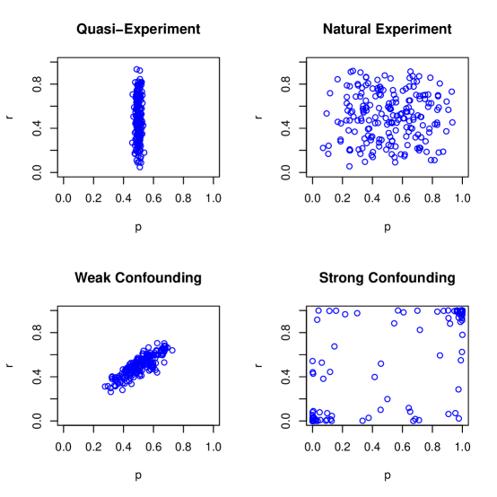
Figure 1. We plot four examples of latent, propensity-risk distributions. These latent distributions are a thought experiment; we do not estimate the latent distributions from data. In the top two figures spurious association is absent because there is no correlation between latent propensity and risk. In the bottom two figures spurious association arises due to correlation between latent propensity and risk. Strong confounding is possible when there is excess variation in propensity and risk, i.e., when $R^{2}$ is large (see Section 2.1). The randomness $\eta=1-R^{2}$ in the Weak Confounding example is $99\%$, while the randomness in the Strong Confounding example is only $13\%$. Measured and unmeasured covariates play a larger role when the distribution is dispersed and a smaller role when the distribution is concentrated near a point. Chance plays a larger role when the distribution is compressed, and in that case assignment to $e$ or $d$ is more “random”. The randomness in the Quasi-Experiment example is $99\%$, and the randomness in the Natural-Experiment example is $83\%$.

2.2. The threshold, $T$, of sufficient randomness

From the observations of $(e,d)$ we know the relative frequencies

$$p_{01}=P(e=0,d=1),\ \ p_{11}=P(e=1,d=1),\ \ p_{00}=P(e=0,d=0),\ \ \textrm{and}\ \ p_{10}=P(e=1,d=0).$$

Let $\mathcal{P}_{0}(S)\subset\mathcal{P}(S)$ be the class of feasible distributions satisfying

$$E[(1-p)r]=p_{01},\quad E[pr]=p_{11},\quad E[(1-p)(1-r)]=p_{00},\quad\textrm{and}\quad E[p(1-r)]=p_{10}.$$

$\mathcal{P}_{0}(S)$ is the set of distributions that are consistent with the observed data (the observed contingency table) under $H_{0}$; see Figure 2.

Figure 2. (a) An illustration of a latent propensity-risk distribution on the $(p,r)$ unit square and (b) the resulting expected relative frequencies. Under $H_{0}$ these expected relative frequencies equal the observed relative frequencies shown in (c). The threshold, $T$, of sufficient randomness is computed under $H_{0}$ by finding the distribution with the largest randomness that is consistent with the observed data; see (2). If our propensity-risk model is accurate and the coefficients of determinism $(R^{2}_{p},R^{2}_{r})$ satisfy $1-R_{p}R_{r}>T$ then we reject $H_{0}$ and causal inference is warranted, i.e., we need to appeal to causality in order to explain the data.

Based on (1), we define the threshold, $T$, of sufficient randomness for causal inference by

(2) $$T:=1-R^{2}_{\star}=1-\min_{\mu\in\mathcal{P}_{0}(S)}R^{2}(\mu)=\max_{\mu\in\mathcal{P}_{0}(S)}\eta(\mu)=\eta^{\star}.$$

$T$ is the maximum amount of randomness that is consistent with the observed data under $H_{0}$. If the coefficients of determinism $(R^{2}_{p},R^{2}_{r})$ satisfy $1-R_{p}R_{r}>T$ then causal inference is warranted.

Remark 2.

The threshold $T$ is computed from the observed data. Specifying $(R^{2}_{p},R^{2}_{r})$ is loosely analogous to specifying the size of a hypothesis test, where size refers to the probability of falsely rejecting a null hypothesis. Computation of $T$ is like computation of a p-value. We may reject $H_{0}$ if $T<1-R_{p}R_{r}$.

To compute $T$ we solve the minimization problem in (2), which can be explicitly written as follows:

(3a) $$R^{2}_{\star}=\min_{\mu\in\mathcal{P}(S)}\ R^{2}(\mu),\qquad\qquad\textrm{where }R^{2}(\mu)=\sqrt{\frac{\sigma^{2}_{p}(\mu)\ \sigma^{2}_{r}(\mu)}{E[p]\ \left(1-E[p]\right)\ E[r]\ \left(1-E[r]\right)}}$$

(3b) such that $$E[(1-p)r]\ =\ p_{01}$$

(3c) $$E[pr]\ =\ p_{11}$$

(3d) $$E[(1-p)(1-r)]\ =\ p_{00}$$

(3e) $$E[p(1-r)]\ =\ p_{10}$$

The objective function is the geometric mean of standardized variances, while the constraint set requires that $\mu$ be a feasible distribution on the $(p,r)$ unit square, i.e., the distribution $\mu$ is required to be consistent with the observed data under $H_{0}$.

3. Results

The following theorem gives an analytic solution to the optimization problem in (3) and hence an explicit formula for the threshold $T$ of sufficient randomness; see (2).

Theorem 3.1.

Suppose $P(e=1)\in(0,1)$ and $P(d=1)\in(0,1)$. Let $p_{01}=P(e=0,d=1)$, $p_{11}=P(e=1,d=1)$, $p_{00}=P(e=0,d=0)$, and $p_{10}=P(e=1,d=0)$. Define

$$\phi:=\frac{p_{11}p_{00}-p_{01}p_{10}}{\sqrt{(p_{11}+p_{10})(p_{00}+p_{10})(p_{01}+p_{11})(p_{01}+p_{00})}}.$$

The threshold, $T$, of sufficient randomness for causal inference can be computed with the following formula:

(4) $$T=1-|\phi|.$$

Theorem 3.1 is proven in Appendix A.1. The quantity $\phi$ is a measure of association known as the $\phi$ coefficient. The $\phi$ coefficient is an analogue of Pearson’s correlation coefficient, $\rho$, but $\phi$ measures association between two dichotomous, categorical variables. The coefficient $\phi$ is related to the chi-squared statistic, and we discuss this connection in Section 5.

We proceed to describe formulas for computing $T$ from the observed prevalence of the exposure, the observed prevalence of the disease, and an observed measure of association. Write the standard (open) 3-simplex

$$\Delta:=\left\{(p_{01},p_{11},p_{00},p_{10})\in\mathbb{R}^{4}\colon\ p_{01},\ p_{11},\ p_{00},\ p_{10}>0;\ \ p_{01}+p_{11}+p_{00}+p_{10}=1\right\}.$$

Denote the marginal relative frequencies by $p_{e}=P(e=1)=p_{11}+p_{10}$ and $p_{d}=P(d=1)=p_{11}+p_{01}$. The set $\Delta$ can be reparametrized with $(p_{e},p_{d},\alpha)$, where $\alpha$ is a measure of association. We have already considered $\alpha=\phi$. Next we consider common measures of association known as the risk difference (RD),

$$RD=\frac{p_{11}}{(p_{11}+p_{10})}-\frac{p_{01}}{(p_{01}+p_{00})},$$

the relative risk (RR),

$$RR=\frac{p_{11}}{(p_{11}+p_{10})}\frac{(p_{01}+p_{00})}{p_{01}},$$

and the odds ratio (OR),

$$OR=\frac{p_{11}}{p_{10}}\frac{p_{00}}{p_{01}}.$$

While Theorem 3.1 gives an explicit formula for $T$ in terms of the relative frequencies of a contingency table, the following proposition (Proposition 3.2) provides formulas for computing $T$ from observed $(p_{e},p_{d},\alpha)$, where $\alpha\in\{RD,RR,OR\}$. We anticipate that it may be useful for gaining intuition for $T$ and during meta analysis of summary statistics.

Proposition 3.2.

Suppose $p_{e},p_{d}\in(0,1)$. Define $k=\sqrt{\frac{p_{e}(1-p_{e})}{p_{d}(1-p_{d})}}$. For $\alpha\in\{RD,RR,OR\}$,

(5) $$T=\begin{cases}1-|RD|k&\textrm{if }\alpha=RD\\ 1-\left|\frac{p_{d}(RR-1)}{1+p_{e}(RR-1)}\right|k&\textrm{if }\alpha=RR\\ 1-\left|\frac{p_{d}(u-1)}{1+p_{e}(u-1)}\right|k&\textrm{if }\alpha=OR,\\ \end{cases}.$$

where $u=\frac{-a+\sqrt{a^{2}-4p_{e}c}}{2p_{e}}$, $a=p_{d}\left(OR-1\right)+\left(1-p_{e}\right)-p_{e}OR$, and $c=(p_{e}-1)OR$.

Proposition 3.2 is proven in Appendix A.2.

Next, we consider $T$ as a sensitivity parameter, and provide a qualitative summary of how $T$ depends on $(p_{e},p_{d},\alpha)$, where $\alpha\in\{RD,RR,OR\}$. We say that a triple $(p_{e},p_{d},\alpha)$ is realizable if it could have resulted from relative frequencies $(p_{01},p_{11},p_{00},p_{10})\in\Delta$. Conditional on $\alpha$ we say that $(p_{e},p_{d})$ is realizable if $(p_{e},p_{d},\alpha)$ is realizable. Conditional on $(p_{e},p_{d})$ we say $\alpha$ is realizable if $(p_{e},p_{d},\alpha)$ is realizable. For $\alpha\in\{RD,RR,OR,\phi\}$ we write $l_{\alpha}$ for the greatest lower bound on realizable $\alpha$, and $u_{\alpha}$ for the least upper bound on realizable $\alpha$. The following lemma presents formulas for $l_{\alpha}$ and $u_{\alpha}$ for $\alpha\in\{RD,RR,OR\}$.

Lemma 3.3.

The triple $(p_{e},p_{d},\alpha)$ is realizable if and only if $p_{e},p_{d}\in(0,1)$ and
for $\alpha=RD$,

$$-1\leq l_{RD}<RD<u_{RD}\leq 1,$$

for $\alpha=RR$,

$$0\leq l_{RR}<RR<u_{RR}\leq\infty,\textrm{~{}or}$$

for $\alpha=OR$,

$$0=l_{OR}<OR<u_{OR}=\infty,$$

where

$$l_{RD} =-\min\left\{\frac{p_{d}}{1-p_{e}},\frac{1-p_{d}}{p_{e}}\right\}, u_{RD}=\min\left\{\frac{p_{d}}{p_{e}},\frac{1-p_{d}}{1-p_{e}}\right\},$$

$$l_{RR} =\max\left\{0,\frac{p_{e}+p_{d}-1}{p_{e}}\right\},\quad\textrm{~{}and~{}} u_{RR}=\begin{cases}\frac{1-p_{e}}{p_{d}-p_{e}}&\textrm{~{}if~{}}p_{e}<p_{d}\\ \infty&\textrm{~{}if~{}}p_{e}\geq p_{d}\end{cases}.$$

Lemma 3.3 is proven in Appendix A.3. The following corollary characterizes how sensitivity depends on association and gives formulas for $l_{\phi}$ and $u_{\phi}$.

Corollary 3.4 (Sensitivity conditional on $(p_{e},p_{d})$).

Given fixed $(p_{e},p_{d})$ with $p_{e},p_{d}\in(0,1)$ we consider realizable triples $(p_{e},p_{d},\alpha)$ for $\alpha\in\{RD,RR,OR\}$. For the purpose of causal inference,

(i) Association is necessary:

If $RD\to 0$, $RR\to 1$, or $OR\to 1$ then $T\to 1$.

(ii) More association is better:

the threshold $T$ is decreasing in each of $|RD|$, $|RR-1|$, and $|OR-1|$.

(iii) Sufficient association may exist:

If $RD\uparrow u_{RD}$, $RR\uparrow u_{RR}$, or $OR\uparrow u_{OR}$ then

$$T\downarrow 1-u_{\phi},\qquad\textrm{where~{}}u_{\phi}:=\sqrt{\min\left\{\frac{p_{e}(1-p_{d})}{p_{d}(1-p_{e})},\frac{p_{d}(1-p_{e})}{p_{e}(1-p_{d})}\right\}}.$$

If $RD\downarrow l_{RD}$, $RR\downarrow l_{RR}$, or $OR\downarrow l_{OR}$ then

$$T\downarrow 1+l_{\phi}\qquad\textrm{where~{}}l_{\phi}:=-\sqrt{\min\left\{\frac{p_{e}p_{d}}{(1-p_{e})(1-p_{d})},\frac{(1-p_{e})(1-p_{d})}{p_{e}p_{d}}\right\}}.$$

Corollary 3.4 is proven in Appendix A.4. Figure 3 shows a graph of $T$ as a function of $RD$, $RR$, and $OR$ and illustrates Corollary 3.4 in the special case of $p_{e}=p_{d}=0.5$. In Corollary 3.4 (iii), $u_{\phi}=1\iff p_{e}=p_{d}$, and $l_{\phi}=-1\iff p_{e}+p_{d}=1$. Sufficient (positive) association exists when $p_{e}=p_{d}$ and sufficient (negative) association exists when $p_{e}+p_{d}=1$. Sufficient association conditional on $(p_{e},p_{d})$ means given any $1-R_{p}R_{r}>0$ there exists a level of association sufficient to warrant causal inference.

Remark 3.

Corollary 3.4 (iii) implies the existence of study designs parameterized by $(p_{e},p_{d},R^{2}_{p},R^{2}_{r})$, with $p_{e}\neq p_{d}$, $p_{e}+p_{d}\neq 1$, and $R_{p}R_{r}>\max\{-l_{\phi},u_{\phi}\}$, so that $\eta=1-R_{p}R_{r}\leq T$ for every realizable association $\alpha$.

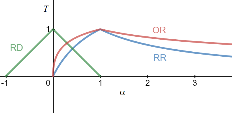
Figure 3. A graph showing $T$ as a function of $\alpha\in\{RD,RR,OR\}$ given $p_{e}=0.5$ and $p_{d}=0.5$. $T\to 0$ as $RR\to\infty$ and as $OR\to\infty$.

We say that a study has a balanced design if $p_{e}$ and $p_{d}$ are near $0.5$. One way to measure the balance of a study design is to use the quantity

(6) $$b=\min\{p_{e},(1-p_{e}),p_{d},(1-p_{d})\}.$$

We can reparametrize $(p_{e},p_{d})\in(0,1)^{2}\setminus\{(0.5,0.5)\}$ with $(b,\theta)$, where $b\in(0,0.5)$ and $\theta\in[0,2\pi)$ is an angle of rotation. The following corollary characterizes how sensitivity depends on $(p_{e},p_{d})$ given $OR$.

Corollary 3.5 (Sensitivity conditional on $OR$).

For the purpose of causal inference, given fixed $OR$ in $(0,\infty)\setminus\{1\}$, and fixed $\theta\in[0,2\pi)$,

(i) Balance is necessary:

If $b\to 0$ then $T\to 1$.

(ii) More balance is better:

The threshold $T$ is decreasing in $b$.

(iii) Sufficient balance does not exist:

For any fixed $OR\in(0,\infty)$,

$$0<\inf_{b\in\{(0,0.5)\}}T.$$

Corollary 3.5 is proven in Appendix A.5. The following corollary characterizes how sensitivity depends on $(p_{e},p_{d})$ given $RD$ and $RR$.

Corollary 3.6 (Sensitivity conditional on $RD$ and $RR$).

For the purpose of causal inference

(i) Sensitivity conditional on $RD$:

For any $RD\in(-1,1)\setminus\{0\}$, on the domain of realizable $(p_{e},p_{d})$, given fixed $p_{e}$ the threshold $T$ is decreasing in $|p_{d}-0.5|$, and given fixed $p_{d}$ the threshold $T$ is increasing in $|p_{e}-0.5|$.

(ii) Sensitivity conditional on $RR$:

For any $RR\in(0,\infty)\setminus\{1\}$, on the domain of realizable $(p_{e},p_{d})$, given fixed $p_{e}$ the threshold $T$ is decreasing in $p_{d}$.

Corollary 3.6 is proven in Appendix A.6. Conditional on $RR$, the dependency of $T$ on $p_{e}$ given fixed $p_{e}$ is more complicated. We demonstrate Corollary 3.5 (ii) with example applications in Section 4.

Corollaries 3.5 and 3.6 are illustrated in Figure 4, where we plot sensitivity conditional on $RD$, $RR$, $OR$, and $\phi$. Conditional on $\phi$ the values of $T$ are constant on the domain of realizable $(p_{e},p_{d})$. Not all $(p_{e},p_{d})$ are realizable conditional on $RD$, $RR$, or $\phi$. All $(p_{e},p_{d})$ are realizable conditional on $OR$.

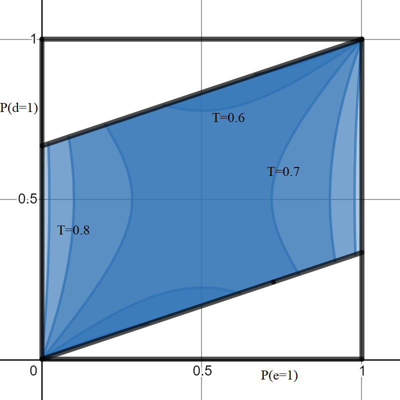
(a) $RD=1/3$

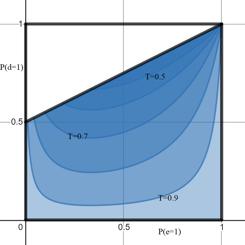
(b) $RR=2$

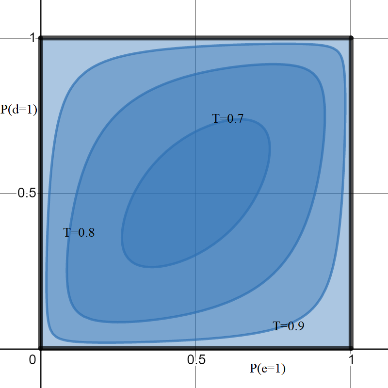
(c) $OR=4$

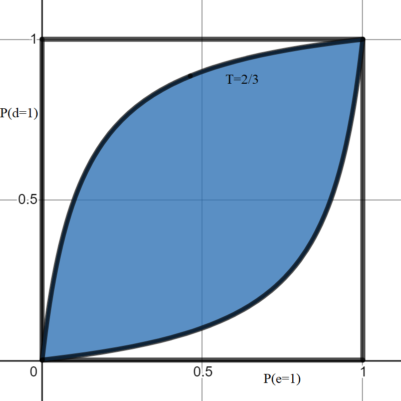
(d) $\phi=1/3$

Figure 4. Conditional on $RD$, $RR$, $OR$, and $\phi$ we plot selected level sets of the sensitivity, $T$, as a function of $(p_{e},p_{d})$. Note that conditional on $\phi$, sensitivity does not depend on realizable $(p_{e},p_{d})$. At $(p_{e},p_{d})=(0.5,0.5)$ the values $RD=1/3$, $RR=2$, $OR=4$, and $\phi=1/3$ are all consistent with $p_{01}=1/6$, $p_{11}=2/6$, $p_{00}=2/6$, and $p_{10}=1/6$, and therefore at $(p_{e},p_{d})=(0.5,0.5)$, by Theorem 3.1, all $T$ values are equal to $1-|\phi|=2/3$. Black curves on the interior of the square indicate the boundaries separating realizable points in blue from unrealizable points in white.

4. Example applications

Here we use the common measure of association $RR$ (relative risk) and Proposition 3.2 to compute the sensitivity $T$ and demonstrate how it depends on more than just strength of association. In our first example application, we analyze a large association only to conclude that it can be explained away with a relatively small $R_{p}R_{r}$ value (see Section 2.1). In our second example application we analyze a much smaller association and find that a slightly larger $R_{p}R_{r}$ value is needed to explain it away. This seeming discrepancy is discussed in more detail within Remark 4 at the conclusion of this section.

4.1. Does diabetes cause stroke?

As part of a World Health Organization (WHO) project Multinational Monitoring of Trends and Determinants of Cardiovascular Disease, Stegmayr and Asplund (1995) studied $119,733$ Swedish women aged 35–74 for eight years. At the start of this cohort study each woman was tested for diabetes mellitus with a glucose test. Any subsequent stroke, as defined by the WHO, was recorded as a primary outcome for each individual under study. Table 1 displays the results. There is a strong, statistically significant, positive association (relative risk RR=5.8; 95% CI 3.7–6.9) between diabetes and stroke.

Table 1. A contingency table showing an observed association (RR $=5.8$) between diabetes and stroke.

	Diabetes
Stroke	No	Yes
Yes	1,823	647
No	110,986	6,277

The exposure $e=1$ is the presence of diabetes at the start of the study and the outcome $d=1$ is any stroke occurrence during the subsequent eight year monitoring time period. From the observed data we compute $P(e=1)=0.058$ and $P(d=1)=0.021$. Using $P(e=1)=0.058$, $P(d=1)=0.021$, and $RR=5.8$ within (5) we compute the threshold $T$ of sufficient randomness to be $\textrm{T}=0.87$. The same quantity can be computed using Theorem 3.1 from the relative frequencies of Table 1,

$$p_{01}=0.015,\quad p_{11}=0.005,\quad p_{00}=0.927,\quad p_{10}=0.053.$$

Assuming the accuracy of our propensity risk model, if $(R^{2}_{p},R^{2}_{r})$ (see Section 2.1) satisfies $1-R_{p}R_{r}>0.87$ then causal inference is warranted.

4.2. Does smoking cause COPD?

The Rotterdam Study is a prospective population-based cohort study in the Netherlands. Researchers have been studying a population of roughly 15,000 residents, each aged greater than or equal to $45$ years and living in a well-defined suburb. They are investigating the occurrence of chronic diseases and risk factors. Terzikhan et al. (2016) have observed a moderate association (relative risk $RR=2.8$) between smoking and chronic obstructive pulmonary disease (COPD). Their raw frequency data is shown in the contingency table shown in Table 2.

Table 2. A contingency table showing an observed association (RR $=2.8$) between smoking and COPD.

	Smoking
COPD	No	Yes
Yes	318	1,631
No	4679	7,538

Here the exposure $e=1$ is a history of smoking, and the outcome $d=1$ is COPD diagnosis via extensive examination at a specially built research facility. From the observed data we compute $P(e=1)=0.647$ and $P(d=1)=0.138$. Using $P(e=1)=0.647$, $P(d=1)=0.138$, and $RR=2.8$ within (5) we compute the threshold $T$ of sufficient randomness to be $\textrm{T}=0.84$. The same quantity can be computed using Theorem 3.1 from the relative frequencies of Table 2,

$$p_{01}=0.02,\quad p_{11}=0.12,\quad p_{00}=0.33,\quad p_{10}=0.53.$$

Assuming the accuracy of our propensity risk model, if $(R^{2}_{p},R^{2}_{r})$ (see Section 2.1) satisfies $1-R_{p}R_{r}>0.84$ then causal inference is warranted.

Remark 4.

In Section 4.1 the measured association was $RR_{\textrm{stroke}}=5.8$, and the scientific question is whether diabetes causes stroke. In Section 4.2 the measured association was $RR_{\textrm{COPD}}=2.8$, and the scientific question is whether smoking causes COPD. Based on the magnitudes of association alone it appears that $RR_{\textrm{stroke}}=5.8$ is more conducive to causal interpretation. However, in Section 4.1 we computed $T_{\textrm{stroke}}=0.87$, and in Section 4.2 we computed $T_{\textrm{COPD}}=0.84$. Based on the thresholds it appears that $RR=2.8$ is more conducive to causal interpretation. The threshold $T_{\textrm{stroke}}$ is higher despite $RR_{\textrm{stroke}}=5.8$ in part because of the rare outcome $P(\textrm{stroke}=1)=0.021$. The threshold $T_{\textrm{COPD}}$ is lower despite $RR_{\textrm{COPD}}=2.8$ in part because of the more common outcome $P(\textrm{COPD}=1)=0.138$. See Figure 4 to appreciate how increasing $p_{d}$ decreases $T$ conditional on $RR$. Thus, the relative risk alone is an inadequate measure of sensitivity, especially when compared with the $\phi$ coefficient of Theorem 3.1 and Figure 4.

5. Discussion

In this paper we have explained how coefficients of determinism $R^{2}_{p}$ and $R^{2}_{r}$ determine the randomness $\eta$ of the data generating process (see Section 2.1). We have also defined a threshold, $T$, of sufficient randomness (see (2)) and demonstrated how to compute $T$ from observed data (see Section 3). If our propensity-risk model is accurate then $1-R_{p}R_{r}>T$ warrants causal inference. However, for causal inference it is not necessary to demonstrate $1-R_{p}R_{r}>T$, as there are many classic approaches to causal inference with demonstrated utility (Pearce et al., 2019). Our introduced methodology is complementary and designed to quantify uncertainty in causal inference from natural experiments and quasi-experiments. The example applications of Section 4 demonstrate the utility of $T$ as an informative sensitivity parameter. We saw how there can be a lower threshold for causal inference despite smaller measured association; see Remark 4.

In the example applications of Section 4 we computed thresholds of sufficient randomness, but we didn’t attempt to specify sets of plausible values for $R^{2}_{p}$ and $R^{2}_{r}$ (see Section 2.1). If our propensity-risk model is appropriate, then $1-R_{p}R_{r}>T$ is sufficient for causal inference, but there may be uncertainty about the set of plausible $(R^{2}_{p},R^{2}_{r})$ values. Specification of plausible values can be based on knowledge of the processes assigning $e$ and $d$, or knowledge of attributes of individuals in the population under study. Care is required when specifying a plausible set for $R^{2}_{r}$ because $r$ is risk in the counterfactual absence of exposure (see Section 2). Separate upper bounds for $R_{p}$ and $R_{r}$ can be multiplied for comparison with $R^{2}_{\star}$ (see (2)). If the resulting product is less than $R^{2}_{\star}$ then causal inference is warranted. This approach is sharp in the following sense: if there is a distribution $\mu\in\mathcal{P}_{0}(S)$ with $R^{2}(\mu)=x$, then for any $(R_{p},R_{r})$ satisfying $0<R_{p},R_{r}<1$ and $R_{p}R_{r}=x$, there exists a distribution $\tilde{\mu}\in\mathcal{P}_{0}(S)$ satisfying $\frac{\sigma^{2}_{p}}{E[p](1-E[p])}=R^{2}_{p}$ and $\frac{\sigma^{2}_{r}}{E[r](1-E[r])}=R^{2}_{r}$. Thus, information is not lost by using $R^{2}=R_{p}R_{r}$ in place of $(R_{p},R_{r})$, and this justifies our use of the geometric mean in definitions for $\eta$ (see Section 2.1) and $T$ (see Section 2.2).

To improve intuition note that increasing variances in propensity or risk can reduce the randomness (see Figure 1). It is best for causal inference when both distributions of propensities and risks have small variance. It is ideal when there is not variance in propensity nor risk. Instead of asking how exposed and unexposed individuals differ with regards to measured and unmeasured covariate data, we are asking how stochastic (i.e., non-deterministic) are the processes assigning exposure and outcome. A partial answer can be obtained from the field of genetics, where measures of heritability are analogous to coefficients of determination (van Rheenen et al., 2019). Instead of adjusting for conveniently measured covariates we can adjust for unmeasured genomic variables by reviewing the literature to bound measures of heritability for the exposure and disease. Note that specification of plausible sets for $R^{2}_{p}$ and $R^{2}_{r}$ is an inexact science, and genomic variables alone are not sufficient for that task, although they can provide lower bounds, and often that will be enough to cast doubt on direct causal inference from the observed association. When both the exposure and disease are highly heritable then causal interpretation of an observed association between exposure and disease may be complicated (c.f. Pearl (2015)).

The following descriptions of studies are examples to help distinguish between studies of insufficient and sufficient randomness. Almond et al. (2010) studied the effectiveness of intensive treatment of low-birth-weight newborns, using a regression discontinuity design. They argue that treatment assignment was “as good as random”, but if measurement error is present then our propensity-risk model indicates that their quasi-experimental design and others like it still have insufficient actual randomness. Perhaps an outcome is more stochastic when longer amounts of time have passed since exposure. While Almond et al. (2010) studied infant morality at one week, one month, and one year, we may think of the outcome at one year as being more stochastic, and therefore the association between treatment and that outcome at one year is more conducive to causal inference, all other things equal. Likewise, in studies of the relative age effect or birthdate effect (Muller and Page, 2015), to the extent that success in sports or life requires luck, or chance, the outcome decades later could be highly stochastic, possibly facilitating causal inference. Finally, with randomized trials that allow patients to switch from control to treatment for ethical reasons (Latimer et al., 2016), it is possible to demonstrate sufficient randomness as long as the proportion of patients who switch treatments is not too large. Simply put, the randomized trial need not be perfect—a warrant for causal inference is provided by sufficient randomness.

The optimization problem of (3) can be reformulated in a variety of equivalent ways. The constraints may be rewritten as $(E[p],E[r],\sigma_{pr})=\left(p_{e},p_{r},\sigma_{ed}\right)$, where $\sigma_{pr}=E[(p-E[p])(r-E[r])]$ is latent covariance and $\sigma_{ed}=p_{01}p_{10}-p_{00}p_{11}$ is the observed covariance. We obtain the same optimal solution with $|\sigma_{pr}|>|\sigma_{ed}|$ in place of $\sigma_{pr}=\sigma_{ed}$. Alternatively, for $\alpha\in\{RD,RR,OR\}$ we may find $\sigma^{\star}_{pr}=\max\{\sigma_{pr}\colon E[p]=p_{e},E[r]=p_{d}\}$ and then use the monotonicity of spurious $\alpha$ as a function of $\sigma_{pr}$ to compute a maximum spurious $\alpha^{\star}$ for comparison with observed $\alpha$. Also, we may define $\rho_{ed}=\phi$ which is consistent with $\phi=\sigma_{ed}/\sqrt{p_{e}(1-p_{e})r_{e}(1-r_{e})}$. Then, given $(E[p],E[r],\sigma_{pr})=(p_{e},p_{d},\sigma_{ed})$ we can factor

$$\sigma_{ed}=\sigma_{pr}=\sigma_{p}\sigma_{r}\rho_{pr} =R_{p}\sqrt{E[p](1-E[p])}R_{r}\sqrt{E[r](1-E[r])}\rho_{pr}$$

(7) $$=R_{p}\sqrt{p_{e}(1-p_{e})}R_{r}\sqrt{p_{d}(1-p_{d})}\rho_{pr}$$

and solve (7) for $R^{2}=R_{p}R_{r}$ to obtain

(8) $$R^{2}=\phi/\rho_{pr}=\rho_{ed}/\rho_{pr}$$

under $H_{0}$, c.f (1). From (8) we then obtain

(9) $$R^{2}_{\star}=\rho_{ed}/\max_{\mathcal{P}_{0}(S)}\{\rho_{pr}\},$$

c.f. (2). Finally, we may express $R^{2}_{\star}$ using the $\chi^{2}$ statistic of the chi-squared test of independence as applied to a $2\times 2$ contingency table without a continuity correction. With a finite sample size $n$ we have

$$\chi^{2} =n\left(\frac{(p_{01}-(1-p_{0})r_{0})^{2}}{(1-p_{0})r_{0}}+\frac{(p_{11}-p_{0}r_{0})^{2}}{p_{0}r_{0}}+\frac{(p_{00}-(1-p_{0})(1-r_{0}))^{2}}{(1-p_{0})(1-r_{0})}+\frac{(p_{10}-p_{0}(1-r_{0}))^{2}}{p_{0}(1-r_{0})}\right)$$

(10) $$=\frac{n(p_{01}p_{10}-p_{11}p_{00})^{2}}{(p_{01}+p_{00})(p_{11}+p_{10})(p_{01}+p_{11})(p_{00}+p_{10})}.$$

Asymptotically, by (2), Theorem 3.1, and (10), we have

(11) $$R^{2}_{\star}=|\phi|=\sqrt{\chi^{2}/n}.$$

By Theorem 3.1 and (11) we see that both the measure of association $\phi$ and the statistic $\chi^{2}$ inform us of the threshold $T$ independent of $(p_{e},p_{d})$.

5.1. Future directions

In this paper, we have introduced a notion of randomness in a simplified setting and there are several interesting future directions that further extend the applicability. Under $H_{0}$ our propensity-risk model assigns $(e,d)$ to individuals, assuming independent assignment. If we eliminate the independence assumption then from any observed $(e,d)$ we can find a feasible latent distribution $\mu\in\mathcal{P}_{0}(S)$ with technically sufficient randomness $1-R^{2}(\mu)\approx 1$, but realistically there would be insufficient randomization if exposure was assigned to the exposed subpopulation at once in mass, for instance. Fisher (1935) speaks of Randomization as the “reasoned basis” for causal inference, and Rosenbaum (2020, p. 37) explains how Fisher’s phrase is in reference to randomization distributions. We could extend our definition of the randomness into the realm of information theory (Cover and Thomas, 2005) and consider entropy as a sensitivity parameter. Causal inference is hindered by lack of independence of observations, insufficient sample size, insufficient randomness of the data generating process, and a lack of balance as defined in (6), and all of these constructs are related to entropy. Our introduced methodology can be adapted for application with smaller sample sizes, and if the sample size is small to moderate we recommend parametric bootstrapping with a multinomial distribution, using the observed probabilities $(p_{01},p_{11},p_{00},p_{10})$ as the parameters, resulting in a bootstrapped distribution of $T$ values.

This paper has emphasized the stochasticity of the data generating process and de-emphasized conditioning on covariates. One way to incorporate measured covariate data into the analysis would be to formulate the constraints conditional on the covariate levels and express $\mu$ as a mixture distribution. With smaller sample sizes we may utilize a transported algorithm to model $r$ (c.f. Rosenbaum et al. (2002, Section 2.3). The randomness $\eta=1-R^{2}$ of the data generating process remains the same, and we could still seek to minimize marginal $R^{2}(\mu)$, thus generalizing the threshold $T$. In some situations conditioning on covariates can increase bias, and it is not always clear how best to proceed (Ding and Miratrix, 2015). Our propensity-risk model provides some insight, and a new perspective—conditioning on covariate data is useful to the extent that it lowers the threshold, $T$, of sufficient randomness for causal inference. If our propensity-risk model of the data generating process is accurate, then any conditioning on measured covariate data can only lower $T$, because $R^{2}_{\star}$ can only increase if the constraint set, $\mathcal{P}_{0}(S)$, is further constrained.

Appendix A Mathematical proofs

A.1. Proof of Theorem 3.1

Write $\mathcal{P}(S)$ for the space of distributions on $S=(0,1)^{2}$ and $\mathcal{P}_{0}(S)\subset\mathcal{P}(S)$ for the class of feasible distributions satisfying the constraints in (3b)–(3e). For a feasible distribution $\mu\in\mathcal{P}_{0}(S)$, the latent covariance is given by

(12a) $$\sigma_{pr} =\int_{S}\left(p-E[p]\right)\left(r-E[r]\right)\ d\mu$$

(12b) $$=\int_{S}pr\ d\mu-E[p]E[r]$$

(12c) $$=p_{11}-\left(p_{10}+p_{11}\right)\left(p_{01}+p_{11}\right)$$

(12d) $$=p_{11}(1-p_{11}-p_{01}-p_{10})-p_{10}p_{01}$$

(12e) $$=p_{11}p_{00}-p_{10}p_{01}$$

(12f) $$=:\sigma_{ed}.$$

Note that in (12c) we used the constraints in (3) and in (12e) we used the fact that $p_{01}+p_{11}+p_{10}+p_{00}=1$. By the Cauchy-Schwarz inequality and (12), any $\mu\in\mathcal{P}_{0}(S)$ satisfies

$$\sigma_{p}^{2}(\mu)\sigma_{r}^{2}(\mu)\geq\sigma_{pr}^{2}(\mu)=\sigma_{ed}^{2}.$$

By (3b)–(3e), any $\mu\in P_{0}(S)$ satisfies

$$E[p]\left(1-E[p]\right)E[r]\left(1-E[r]\right)\ =\ p_{e}(1-p_{e})p_{d}(1-p_{d}),$$

where $p_{e}=P(e=1)$ and $p_{d}=P(d=1)$. Thus, we have that any $\mu\in P_{0}(S)$ satisfies

(13) $$R^{2}(\mu)\geq\frac{|\sigma_{ed}|}{\sqrt{p_{e}p_{d}(1-p_{e})(1-p_{d})}}.$$

It remains to show that there exists a feasible probability distribution, $\mu\in\mathcal{P}_{0}(S)$ that attains the lower bound in (13). Write the signum function $\operatorname{sgn}(x)=\begin{cases}1&\textrm{if~{}}x>0\\ 0&\textrm{if~{}}x=0\\ -1&\textrm{if~{}}x<0\end{cases}$ and define

$$\theta_{1} =\min\left\{p_{e},\frac{1}{2}+\operatorname{sgn}\left(\sigma_{ed}\right)\left(p_{d}-\frac{1}{2}\right)\right\}=\begin{cases}\min\{p_{e},p_{d}\}&\textrm{~{}if~{}}\sigma_{ed}>0\\ \min\{p_{e},\frac{1}{2}\}&\textrm{~{}if~{}}\sigma_{ed}=0\\ \min\{p_{e},1-p_{d}\}&\textrm{~{}if~{}}\sigma_{ed}<0\end{cases}$$

$$\theta_{2} =\min\left\{1-p_{e},\frac{1}{2}+\operatorname{sgn}\left(\sigma_{ed}\right)\left(\frac{1}{2}-p_{d}\right)\right\}=\begin{cases}\min\{1-p_{e},1-p_{d}\}&\textrm{~{}if~{}}\sigma_{ed}>0\\ \min\{1-p_{e},\frac{1}{2}\}&\textrm{~{}if~{}}\sigma_{ed}=0\\ \min\{1-p_{e},p_{d}\}&\textrm{~{}if~{}}\sigma_{ed}<0\end{cases}.$$

We claim that the lower bound in (13) is attained by the two point-mass distribution

$$\mu^{\star}(p,r)=\frac{\theta_{1}}{\theta_{1}+\theta_{2}}\delta(p-p_{1},r-r_{1})+\frac{\theta_{2}}{\theta_{1}+\theta_{2}}\delta(p-p_{2},r-r_{2}),$$

where $\delta(p,r)$ is the Dirac delta distribution and

$$(p_{1},r_{1}) :=\left(p_{e}+k_{1},\ p_{d}+\operatorname{sgn}(\sigma_{ed})k_{1}\right),\qquad k_{1}:=\sqrt{\frac{\theta_{2}}{\theta_{1}}}\sqrt{|\sigma_{ed}|}$$

$$(p_{2},r_{2}) :=\left(p_{e}-k_{2},\ p_{d}-\operatorname{sgn}(\sigma_{ed})k_{2}\right),\qquad k_{2}:=\sqrt{\frac{\theta_{1}}{\theta_{2}}}\sqrt{|\sigma_{ed}|}.$$

We first claim that $(p_{1},r_{1})\in S$ and $(p_{2},r_{2})\in S$ so that $\int_{S}d\mu^{\star}=1$, i.e., $\mu^{\star}\in\mathcal{P}(S)$. If $\sigma_{ed}=0$, then $k_{1}=k_{2}=0$, so $(p_{1},r_{1})=(p_{2},r_{2})=(p_{e},p_{d})\in S$. Now assume $\sigma_{ed}\neq 0$. We claim that

(14) $$-\min\{p_{e}p_{d},(1-p_{e})(1-p_{d})\}<\sigma_{ed}<\min\{p_{e}(1-p_{d}),p_{d}(1-p_{e})\}.$$

To see (14), we first compute $\sigma_{pr}=\int_{S}\left(p-p_{e}\right)\left(r-p_{d}\right)\ d\mu=\int_{S}pr\ d\mu-p_{e}p_{d}$. Since $(p,r)\in(0,1)^{2}$, we have that $\int_{S}pr\ d\mu<\min\{p_{e},p_{d}\}$, from which the claimed upper bound in (14) follows. We also have that $\int_{S}pr\ d\mu>0$, so that $\sigma_{pr}>-p_{e}p_{d}$. Finally from the identity $\sigma_{pr}=\int_{S}(1-p)(1-r)\ d\mu-(1-p_{e})(1-p_{d})$ and the observation that $\int_{S}(1-p)(1-r)\ d\mu>0$, we have that $\sigma_{pr}>-(1-p_{e})(1-p_{d})$. Putting these two inequalities together gives the claimed lower bound in (14). With $\sigma_{ed}\neq 0$ we have

$$\theta_{1}\theta_{2}=\begin{cases}\min\{p_{e}(1-p_{d}),p_{d}(1-p_{e})\}\textrm{~{}if~{}}\sigma_{ed}>0\\ \min\{p_{e}p_{d},(1-p_{e})(1-p_{d})\}\textrm{~{}if~{}}\sigma_{ed}<0\end{cases}$$

and from (14) we then have $\theta_{1}\theta_{2}>|\sigma_{ed}|$ so that $k_{1}=\theta_{2}\sqrt{\frac{|\sigma_{ed}|}{\theta_{1}\theta_{2}}}<\theta_{2}$ and $k_{2}=\theta_{1}\sqrt{\frac{|\sigma_{ed}|}{\theta_{1}\theta_{2}}}<\theta_{1}$. Because $k_{1}<\theta_{2}$ and $k_{2}<\theta_{1}$ we have $(p_{1},r_{1})\in S$ and $(p_{2},r_{2})\in S$.

We now verify that $\mu^{\star}$ satisfies the constraints in (3b)–(3e). We first compute

$$\int_{S}pr\ d\mu^{\star}=\frac{\theta_{1}}{\theta_{1}+\theta_{2}}p_{1}r_{1}+\frac{\theta_{2}}{\theta_{1}+\theta_{2}}p_{2}r_{2}=p_{e}p_{d}+\sigma_{ed}=p_{11},$$

which verifies (3c). We then compute

$$\int_{S}p\ d\mu^{\star}=\frac{\theta_{1}}{\theta_{1}+\theta_{2}}p_{1}+\frac{\theta_{2}}{\theta_{1}+\theta_{2}}p_{2}=p_{e}+\frac{\theta_{1}k_{1}-\theta_{2}k_{2}}{\theta_{1}+\theta_{2}}=p_{e}\quad\textrm{and similarly}\quad\int_{S}r\ d\mu^{\star}=p_{d}.$$

This gives us that

$$\int_{S}(1-p)r\ d\mu^{\star}=p_{d}-p_{11}=p_{01}$$

$$\int_{S}p(1-r)\ d\mu^{\star}=p_{e}-p_{11}=p_{10}$$

$$\int_{S}(1-p)(1-r)\ d\mu^{\star}=1-p_{e}-p_{d}+p_{11}=p_{00},$$

which verifies (3b), (3d), and (3e).

To evaluate $R^{2}(\mu^{\star})$, we compute

$$\sigma_{p}^{2}=\frac{\theta_{1}}{\theta_{1}+\theta_{2}}(p_{1}-p_{e})^{2}+\frac{\theta_{2}}{\theta_{1}+\theta_{2}}(p_{2}-p_{e})^{2}=\frac{\theta_{1}k_{1}^{2}+\theta_{2}k_{2}^{2}}{\theta_{1}+\theta_{2}}=|\sigma_{ed}|$$

and similarly $\sigma_{r}^{2}=|\sigma_{ed}|$. Then

$$R^{2}(\mu^{\star})=\frac{|\sigma_{ed}|}{\sqrt{p_{e}\left(1-p_{e}\right)p_{d}\left(1-p_{d}\right)}}$$

which together with (13) establishes that $\min_{\mu\in\mathcal{P}_{0}(S)}R^{2}(\mu)=|\phi|$. From the definition of $T$ in (2), this establishes (4). $\blacksquare$

A.2. Proof of Proposition 3.2

For each measure of association, $\alpha\in\{RD,RR,OR\}$, we derive the formula in (5).

$\alpha=RD$. By definition, $RD=\frac{p_{11}}{p_{11}+p_{10}}-\frac{p_{01}}{p_{00}+p_{01}}$ so

$$p_{e}(1-p_{e})RD=(p_{00}+p_{01})p_{11}-(p_{11}+p_{10})p_{01}=p_{00}p_{11}-p_{10}p_{01}=\phi\sqrt{p_{e}(1-p_{e})p_{d}(1-p_{d})}$$

So we have that $k|RD|=|\phi|$, so $T=1-|\phi|=1-|RD|k$, as desired.

$\alpha=RR$. Using the definition of $RR$, we have

$$RR-1 =\frac{p_{11}}{p_{e}}-\frac{1-p_{e}}{p_{01}}-1=\frac{p_{11}-p_{e}p_{d}}{p_{e}p_{01}}$$

$$p_{d}(RR-1) =\frac{p_{d}}{p_{e}}\frac{p_{11}-p_{e}p_{d}}{p_{01}}$$

$$1+p_{e}(RR-1) =\frac{p_{d}(1-p_{e})}{p_{01}}.$$

Dividing these last two quantities, we obtain

$$\frac{p_{d}(RR-1)}{1+p_{e}(RR-1)}=\frac{p_{11}-p_{e}p_{d}}{p_{e}(1-p_{e})}.$$

On the other hand,

$$RD=\frac{p_{11}}{p_{e}}-\frac{p_{01}}{1-p_{e}}=\frac{p_{11}(1-p_{e})-p_{01}p_{e}}{p_{e}(1-p_{e})}=\frac{p_{11}-p_{e}p_{d}}{p_{e}(1-p_{e})}.$$

Combining these last two expressions, we have that

$$RD=\frac{p_{d}(RR-1)}{1+p_{e}(RR-1)},$$

which together with the expression $T=1-|RD|k$ gives the desired result.

$\alpha=OR$. We compute

(15) $$\frac{OR}{RR} =\frac{p_{00}}{p_{10}}\frac{(p_{10}+p_{11})}{(p_{01}+p_{00})}$$

$$=\frac{p_{10}p_{00}+p_{10}p_{01}-p_{10}p_{01}+p_{00}p_{11}}{p_{10}p_{01}+p_{10}p_{00}}$$

$$=1-\frac{p_{10}p_{01}}{p_{10}p_{00}+p_{10}p_{01}}+\frac{p_{00}}{p_{10}}\left(\frac{p_{11}}{p_{00}+p_{01}}\right)$$

$$=1-\frac{p_{01}}{p_{00}+p_{01}}+\frac{p_{01}}{p_{00}+p_{01}}OR.$$

Rearranging, we obtain

(16) $$RR=\frac{OR}{1-\frac{p_{01}}{p_{01}+p_{00}}+\frac{p_{01}}{p_{01}+p_{00}}OR}.$$

We proceed to express $\frac{p_{01}}{p_{01}+p_{00}}$ in terms of $RR$, $p_{e}$, and $p_{d}$. By the definition of $RR$ we have

(17) $$RR=\frac{p_{11}}{p_{01}}\frac{(1-p_{e})}{p_{e}}.$$

From (17) and $p_{d}=p_{01}+p_{11}$ we solve for

$$p_{01}=\frac{p_{d}(1-p_{e})}{1+p_{e}(RR-1)}$$

and then divide by $p_{01}+p_{00}=1-p_{e}$ to obtain

(18) $$\frac{p_{01}}{p_{01}+p_{00}}=\frac{p_{d}}{1+p_{e}(RR-1)}.$$

By combining (16) and (18) we obtain

(19) $$p_{e}RR^{2}+(p_{d}(OR-1)+(1-p_{e})-p_{e}OR)RR-(1-p_{e})OR=0.$$

Writing $a=p_{d}\left(OR-1\right)+\left(1-p_{e}\right)-p_{e}OR$ and $c=(p_{e}-1)OR$, we apply the quadratic formula to find that

$$RR=u_{\pm}:=\frac{-a\pm\sqrt{a^{2}-4p_{e}c}}{2p_{e}}.$$

The discriminant is clearly positive since $a^{2}-4p_{e}c=a^{2}+4p_{e}(1-p_{e})OR\geq 0$ so we have two real roots. To choose the sign, we insist that $RR=1$ when $OR=1$, which requires the plus sign in the quadratic formula. Now combining the result with the formula for $T(\alpha)$ with $\alpha=RR$ in (5), we obtain the desired formula. $\blacksquare$

A.3. Proof of Lemma 3.3

We can express the measures of association $RD$, $RR$, and $OR$ in terms of the covariance $\sigma_{ed}:=p_{11}p_{00}-p_{10}p_{01}$ as follows:

(20a) $$RD =\frac{p_{e}p_{d}+\sigma_{ed}}{p_{e}p_{d}+p_{e}(1-p_{d})}-\frac{(1-p_{e})p_{d}-\sigma_{ed}}{(1-p_{e})p_{d}+(1-p_{e})(1-p_{d})}$$

(20b) $$RR =\frac{p_{e}p_{d}+\sigma_{ed}}{p_{e}p_{d}+p_{e}(1-p_{d})}\frac{(1-p_{e})p_{d}+(1-p_{e})(1-p_{d})}{(1-p_{e})p_{d}-\sigma_{ed}}$$

(20c) $$OR =\frac{(p_{e}p_{d}+\sigma_{ed})((1-p_{e})(1-p_{d})+\sigma_{ed})}{(p_{e}(1-p_{d})-\sigma_{ed})((1-p_{e})p_{d}-\sigma_{ed})}.$$

From (14), we have $\sigma_{ed}\in(l_{\sigma},u_{\sigma})$, where

$$l_{\sigma}=-\min\{p_{e}p_{d},(1-p_{e})(1-p_{d})\}\qquad\textrm{and}\qquad u_{\sigma}:=\min\{p_{e}(1-p_{d}),p_{d}(1-p_{e})\}.$$

Moreover, it is possible to construct sequences of contingency tables such that $\sigma_{ed}$ approaches these lower and upper bounds. Now, using the continuity and monotonicity of each of $RD$, $RR$, and $OR$ in $\sigma_{ed}$, we can compute upper and lower bounds for each of these measures of association

(21a) $$u_{RD} =\lim_{\sigma_{ed}\to u_{\sigma}}RD=\begin{cases}&\frac{p_{d}}{p_{e}}\textrm{~{}if~{}}p_{e}\geq p_{d}\\ &\frac{1-p_{d}}{1-p_{e}}\textrm{~{}if~{}}p_{e}<p_{d}\end{cases},$$

(21b) $$l_{RD} =\lim_{\sigma_{ed}\to l_{\sigma}}RD=\begin{cases}&\frac{p_{d}-1}{p_{e}}\textrm{~{}if~{}}p_{e}+p_{d}\geq 1\\ &\frac{p_{d}}{p_{e}-1}\textrm{~{}if~{}}p_{e}+p_{d}<1\end{cases},$$

(21c) $$u_{RR} =\lim_{\sigma_{ed}\to u_{\sigma}}RR=\begin{cases}&\infty\textrm{~{}if~{}}p_{e}\geq p_{d}\\ &\frac{1-p_{e}}{p_{d}-p_{e}}\textrm{~{}if~{}}p_{e}<p_{d}\end{cases},$$

(21d) $$l_{RR} =\lim_{\sigma_{ed}\to l_{\sigma}}RR=\begin{cases}&\frac{p_{e}+p_{d}-1}{p_{e}}\textrm{~{}if~{}}p_{e}+p_{d}\geq 1\\ &0\textrm{~{}if~{}}p_{e}+p_{d}<1\end{cases},$$

(21e) $$u_{OR} =\lim_{\sigma_{ed}\to u_{\sigma}}OR=\infty,\textrm{~{}and}$$

(21f) $$l_{OR} =\lim_{\sigma_{ed}\to l_{\sigma}}OR=0.$$

Combining the cases completes the proof. $\blacksquare$

A.4. Proof of Corollary 3.4

From (5), with $k=\sqrt{\frac{p_{e}(1-p_{e})}{p_{d}(1-p_{d})}}$, we have

$$T(\alpha)=\begin{cases}1-|RD|k&\textrm{if }\alpha=RD\\ 1-|\frac{p_{d}(RR-1)}{1+p_{e}(RR-1)}|k&\textrm{if }\alpha=RR\\ 1-|\frac{p_{d}(u-1)}{1+p_{e}(u-1)}|k&\textrm{if }\alpha=OR\\ \end{cases},$$

where $u=\frac{-a+\sqrt{a^{2}-4p_{e}c}}{2p_{e}}$, $a=p_{d}\left(OR-1\right)+\left(1-p_{e}\right)-p_{e}OR$, and $c=(p_{e}-1)OR$. It can be checked that $u=1$ at $OR=1$.

(i) Association is necessary:

Since $T$ is a continuous function of $RD$, $RR$, and $OR$, we have

$\alpha=RD$:

$\lim_{RD\to 0}T(RD)=T(0)=1$,

$\alpha=RR$:

$\lim_{RR\to 1}T(RR)=T(1)=1$,

$\alpha=OR$:

$\lim_{OR\to 1}T(OR)=T(1)=1$.

(ii) Stronger associations are better:

For $\alpha=RD$, since $k>0$ it is clear that $T$ is decreasing in $\left|RD\right|.$

For $\alpha=RR$, from (5), we consider two cases: $RR>1$ and $RR<1$. If $RR>1$, we have

$$T(RR)=1-\frac{p_{d}|RR-1|}{1+p_{e}|RR-1|}k=f_{1}(|RR-1|),$$

where $f_{1}(x)=1-\frac{p_{d}x}{1+p_{e}x}k$. It is easy to check that $f_{1}^{\prime}(x)<0$ for $x>0$. Similarly, for $RR<1$, we have

$$T(RR)=1-\frac{p_{d}|RR-1|}{1-p_{e}|RR-1|}k=f_{2}(|RR-1|),$$

where $f_{2}(x)=1+\frac{p_{d}x}{1-p_{e}x}k$. Again, it is easy to check that $f_{2}^{\prime}(x)<0$ for $x>0$.

For $\alpha=OR$, we use the result for $\alpha=RR$, that RR and OR are monotonically varying together (see (15)), and $RR=1$ if and only if $OR=1$.

(iii) Sufficient association may exist:

This proof follows from Lemma 3.3 and its proof. Recall the definition from (12f) that $\sigma_{ed}:=p_{11}p_{00}-p_{10}p_{01}$. Rewriting (4) results in

(22) $$T=1-\frac{|\sigma_{ed}|}{\sqrt{p_{e}p_{d}(1-p_{e})(1-p_{d})}}.$$

If $RD\uparrow u_{RD}$, $RR\uparrow u_{RR}$, or $OR\uparrow u_{OR}$ then by (20) and (21) we have $\sigma_{ed}\uparrow u_{\sigma}=\min\{p_{e}(1-p_{d}),p_{d}(1-p_{e})\}$, and from (22) we conclude

$$T\downarrow 1-\sqrt{\min\left\{\frac{p_{e}(1-p_{d})}{p_{d}(1-p_{e})},\frac{p_{d}(1-p_{e})}{p_{e}(1-p_{d})}\right\}}=1-u_{\phi},$$

as desired. Likewise, if $RD\downarrow l_{RD}$, $RR\downarrow l_{RR}$, or $OR\downarrow l_{OR}$ then by (20) and (21) we have $\sigma_{ed}\downarrow l_{\sigma}=-\min\{p_{e}p_{d},(1-p_{e})(1-p_{d}\}$, and from (22) we conclude

$$T\downarrow 1-\sqrt{\min\left\{\frac{p_{e}p_{d}}{(1-p_{e})(1-p_{d})},\frac{(1-p_{e})(1-p_{d})}{p_{e}p_{d}}\right\}}=1+l_{\phi},$$

as desired. $\blacksquare$

A.5. Proof of Corollary 3.5

In this proof, we will use symmetry properties of $T$ and $OR$ several times. $T$ and $OR$ are both invariant under either of the following transformations:

$$(p_{01},p_{10})\mapsto(p_{10},p_{01})$$

$$(p_{00},p_{11})\mapsto(p_{11},p_{00}).$$

Also, either of the transformations $p_{e}\mapsto(1-p_{e})$ and $p_{d}\mapsto(1-p_{d})$ take $OR$ to $1/OR$. These can seen from (4) and the definition of the odds ratio.

(i) Balance is necessary:

Using the above symmetry properties of $T$ and $OR$, without loss of generality, we may assume that $OR>1\iff RR\geq 1$ and $p_{d}\geq p_{e}$. Rearrangement of (19) gives

$$p_{e}(RR-1)^{2}+\left(1+(p_{d}-p_{e})(OR-1)\right)(RR-1)-(1-p_{d})(OR-1)=0.$$

With $h=(OR-1)$ we then have

$$RR-1=\frac{-(1+(p_{d}-p_{e})h)+\sqrt{(1+(p_{d}-p_{e})h)^{2}+4hp_{e}(1-p_{d})}}{2p_{e}}.$$

Then from (5) with $\alpha=RR$ and assuming that $RR\geq 1$ we have

(23) $$1-T=\frac{\sqrt{(1+(p_{d}-p_{e})h)^{2}+4hp_{e}(1-p_{d})}-(1+(p_{d}-p_{e})h)}{2+\sqrt{(1+(p_{d}-p_{e})h)^{2}+4hp_{e}(1-p_{d})}-(1+(p_{d}-p_{e})h)}\sqrt{\frac{p_{d}(1-p_{e})}{p_{e}(1-p_{d})}}.$$

If either $p_{e}\to 0$ or $p_{d}\to 1$ then $T\to 1$ because, by l’Hôpital’s rule,

$$\frac{\sqrt{(1+(p_{d}-p_{e})h)^{2}+4hp_{e}(1-p_{d})}-(1+(p_{d}-p_{e})h)}{\sqrt{p_{e}(1-p_{d})}}\to 0,$$

and

$$\frac{\sqrt{p_{d}(1-p_{e})}}{2+\sqrt{(1+(p_{d}-p_{e})h)^{2}+4hp_{e}(1-p_{d})}-(1+(p_{d}-p_{e})h)}$$

is bounded.

(ii) More balance is better:

Define $v_{1}=p_{e}+p_{d}-1$ and $v_{2}=p_{e}-p_{d}$ so that $p_{e}=(v_{1}+v_{2}+1)/2$ and $p_{d}=(v_{1}-v_{2}+1)/2$. Using the above symmetry properties of $T$ and $OR$, without loss of generality, we may assume that $OR>1\iff RR>1$, $v_{1}\geq 0$, $v_{2}\geq 0$, and $v_{1}+v_{2}<1$. It suffices to show, for $i=1,2$, that $1-T$ is strictly decreasing in $v_{i}$ if $v_{i}>0$.

Writing $h=OR-1$, we obtain from (23),

$$1-T =\frac{\sqrt{1+h((h+1)v_{2}^{2}+1-v_{1}^{2})}+hv_{2}-1}{\sqrt{1+h((h+1)v_{2}^{2}+1-v_{1}^{2})}+hv_{2}+1}\sqrt{\frac{(1-v_{2})^{2}-v_{1}^{2}}{(1+v_{2})^{2}-v_{1}^{2}}}$$

$$=\frac{A-1}{A+1}B,$$

where $A:=\sqrt{1+h((h+1)v_{2}^{2}+1-v_{1}^{2})}+hv_{2}>1$ and $B:=\sqrt{\frac{(1-v_{2})^{2}-v_{1}^{2}}{(1+v_{2})^{2}-v_{1}^{2}}}>0$. We compute

(24) $$\frac{\partial}{\partial v_{i}}(1-T)=\frac{2B}{(A+1)^{2}}\frac{\partial A}{\partial v_{i}}+\frac{A-1}{A+1}\frac{\partial B}{\partial v_{i}},\qquad i=1,2.$$

If $v_{1}>0$ then

$$\frac{\partial A}{\partial v_{1}} =-\frac{hv_{1}}{A}<0$$

$$\frac{\partial B}{\partial v_{1}} =-\frac{v_{1}(1/B-B)}{(1+v_{2})^{2}-v_{1}^{2}}<0,$$

and $1-T$ is strictly decreasing in $v_{1}$.

We also have

$$\frac{\partial A}{\partial v_{2}} =h+\frac{h(h+1)v_{2}}{A}>0$$

$$\frac{\partial B}{\partial v_{2}} =-\frac{(1-v_{2})\frac{1}{B}+(1+v_{2})B}{(1+v_{2})^{2}-v_{1}^{2}}<0.$$

If $v_{2}>0$ then we use (24) and show that $f>0$, where

$$f:=-A\frac{(A+1)^{2}}{2B}\frac{\partial}{\partial v_{2}}(1-T)=A(A^{2}-1)C-Ah-h(h+1)v_{2}$$

and

$$C:=-\frac{1}{2B}\frac{\partial B}{\partial v_{2}}=\frac{1-v_{1}^{2}-v_{2}^{2}}{\left((1-v_{2})^{2}-v_{1}^{2}\right)\left((1+v_{2})^{2}-v_{1}^{2}\right)}\geq 1.$$

We will first show that $f$ is increasing in $v_{2}$, i.e., $\frac{\partial f}{\partial v_{2}}>0$. Using $A(A^{2}-1)\geq 0$ and $\frac{\partial C}{\partial v_{2}}\geq 0$, we compute

(25a) $$\frac{\partial f}{\partial v_{2}} =[(3A^{2}-1)C-h]\frac{\partial A}{\partial v_{2}}+A(A^{2}-1)\frac{\partial C}{\partial v_{2}}-h(h+1)$$

(25b) $$\geq[(A^{2}-1)C-h]\frac{\partial A}{\partial v_{2}}+2A^{2}C\frac{\partial A}{\partial v_{2}}-h(h+1).$$

We now use the inequality

$$A^{2}-1=h(v_{2}^{2}+1-v_{1}^{2}+2v_{2}A)\geq h(1-v_{1}^{2})$$

and the fact that $C\geq\frac{1}{1-v_{1}^{2}}$ to conclude that $(A^{2}-1)C\geq h$. From (25), $\frac{\partial A}{\partial v_{2}}\geq h$, and $C\geq 1$ we have

$$\frac{\partial f}{\partial v_{2}} \geq 2(h+C)h-h(h+1)\geq h(h+1)>0.$$

Since $f$ is increasing in $v_{2}$ and $f\big{|}_{v_{2}=0}=0$ we have $f>0$ if $v_{2}>0$.

(iii) Sufficient balance does not exist:

If $OR=1$ then $T=1>0$ for each $(p_{e},p_{d})\in(0,1)^{2}$. If $OR\neq 1$, by Corollary 3.5(ii) we have that $T$ is decreasing in $b$ for any $b\in(0,0.5)$. Using the continuity of $T$ in $b$, we have that

$$\inf_{b\in(0,0.5)}T=T(p_{e}=0.5,p_{d}=0.5).$$

From (23) we know for any $OR>1$ that

$$1-T(p_{e}=0.5,p_{d}=0.5)=\frac{\sqrt{OR}-1}{\sqrt{OR}+1}<1,$$

which implies that $T(p_{e}=0.5,p_{d}=0.5)>0$. By symmetry, the result also holds for $OR<1$. $\blacksquare$

A.6. Proof of Corollary 3.6

(i) Sensitivity conditional on $RD$:

We have fixed $RD\in(-1,1)\setminus\{0\}$. From (5), we have

$$T=1-\left|RD\right|k=1-\left|RD\right|\sqrt{p_{e}(1-p_{e})}\frac{1}{\sqrt{p_{d}(1-p_{d})}}=1-\left|RD\right|\sqrt{p_{e}(1-p_{e})}\frac{1}{\sqrt{\frac{1}{4}-\left|p_{d}-\frac{1}{2}\right|^{2}}},$$

which is decreasing in $\left|p_{d}-\frac{1}{2}\right|$. Similarly, we have

$$T=1-\left|RD\right|\sqrt{\frac{1}{4}-\left|p_{e}-\frac{1}{2}\right|^{2}}\frac{1}{\sqrt{p_{d}(1-p_{d})}},$$

which is increasing in $\left|p_{e}-\frac{1}{2}\right|$.

(ii) Sensitivity conditional on $RR$:

We have fixed $RR\in(0,\infty)\setminus\{1\}$. From (5), we have

$$T=1-\left|\frac{p_{d}(RR-1)}{1+p_{e}(RR-1)}\right|k=1-\left|\frac{(RR-1)}{1+p_{e}(RR-1)}\right|\sqrt{p_{e}(1-p_{e})}\sqrt{\frac{p_{d}}{(1-p_{d})}},$$

which is decreasing in $p_{d}$ on $(0,1)$. $\blacksquare$

References

- Almond et al. [2010] D. Almond, J. Joseph J. Doyle, A. E. Kowalski, and H. Williams. Estimating marginal returns to medical care: Evidence from at-risk newborns. Quarterly Journal of Economics, 125(2):591–634, may 2010. doi: 10.1162/qjec.2010.125.2.591. URL https://doi.org/10.1162%2Fqjec.2010.125.2.591.
- Cinelli and Hazlett [2019] C. Cinelli and C. Hazlett. Making sense of sensitivity: extending omitted variable bias. Journal of the Royal Statistical Society: Series B (Statistical Methodology), 82(1):39–67, dec 2019. doi: 10.1111/rssb.12348. URL https://doi.org/10.1111%2Frssb.12348.
- Cover and Thomas [2005] T. M. Cover and J. A. Thomas. Elements of Information Theory. Wiley, apr 2005. doi: 10.1002/047174882x. URL https://doi.org/10.1002%2F047174882x.
- Ding and Miratrix [2015] P. Ding and L. W. Miratrix. To adjust or not to adjust? sensitivity analysis of m-bias and butterfly-bias. Journal of Causal Inference, 3(1):41–57, mar 2015. doi: 10.1515/jci-2013-0021. URL https://doi.org/10.1515%2Fjci-2013-0021.
- Ding and VanderWeele [2016] P. Ding and T. J. VanderWeele. Sensitivity analysis without assumptions. Epidemiology, 27(3):368–377, may 2016. doi: 10.1097/ede.0000000000000457. URL https://doi.org/10.1097%2Fede.0000000000000457.
- Fisher [1935] R. A. Fisher. Design of Experiments. Oliver and Boyd, 1935.
- Frank [2000] K. A. Frank. Impact of a confounding variable on a regression coefficient. Sociological Methods & Research, 29(2):147–194, nov 2000. doi: 10.1177/0049124100029002001. URL https://doi.org/10.1177%2F0049124100029002001.
- Hosman et al. [2010] C. A. Hosman, B. B. Hansen, and P. W. Holland. The sensitivity of linear regression coefficients’ confidence limits to the omission of a confounder. The Annals of Applied Statistics, 4(2):849–870, jun 2010. doi: 10.1214/09-aoas315. URL https://doi.org/10.1214%2F09-aoas315.
- Knaeble and Dutter [2017] B. Knaeble and S. Dutter. Reversals of least-square estimates and model-invariant estimation for directions of unique effects. The American Statistician, 71(2):97–105, apr 2017. doi: 10.1080/00031305.2016.1226951. URL https://doi.org/10.1080%2F00031305.2016.1226951.
- Knaeble et al. [2020] B. Knaeble, B. Osting, and M. Abramson. Regression analysis of unmeasured confounding. Epidemiologic Methods, 9(1), may 2020. doi: 10.1515/em-2019-0028. URL https://doi.org/10.1515%2Fem-2019-0028.
- Latimer et al. [2016] N. R. Latimer, C. Henshall, U. Siebert, and H. Bell. Treatment switching: Statistical and decision-making challenges and approaches. International Journal of Technology Assessment in Health Care, 32(3):160–166, 2016. doi: 10.1017/s026646231600026x. URL https://doi.org/10.1017%2Fs026646231600026x.
- Muller and Page [2015] D. Muller and L. Page. Born leaders: political selection and the relative age effect in the US congress. Journal of the Royal Statistical Society: Series A (Statistics in Society), 179(3):809–829, dec 2015. doi: 10.1111/rssa.12154. URL https://doi.org/10.1111%2Frssa.12154.
- Oster [2017] E. Oster. Unobservable selection and coefficient stability: Theory and evidence. Journal of Business & Economic Statistics, 37(2):187–204, jun 2017. doi: 10.1080/07350015.2016.1227711. URL https://doi.org/10.1080%2F07350015.2016.1227711.
- Pearce et al. [2019] N. Pearce, J. P. Vandenbroucke, and D. A. Lawlor. Causal inference in environmental epidemiology: Old and new approaches. Epidemiology, 30(3):311–316, may 2019. doi: 10.1097/ede.0000000000000987. URL https://doi.org/10.1097%2Fede.0000000000000987.
- Pearl [2015] J. Pearl. Comment on ding and miratrix: “to adjust or not to adjust?”. Journal of Causal Inference, 3(1):59–60, mar 2015. doi: 10.1515/jci-2015-0004. URL https://doi.org/10.1515%2Fjci-2015-0004.
- Rosenbaum [2002] P. R. Rosenbaum. Observational Studies. Springer New York, 2002. doi: 10.1007/978-1-4757-3692-2. URL https://doi.org/10.1007%2F978-1-4757-3692-2.
- Rosenbaum [2020] P. R. Rosenbaum. Design of Observational Studies. Springer International Publishing, 2020. doi: 10.1007/978-3-030-46405-9. URL https://doi.org/10.1007%2F978-3-030-46405-9.
- Rosenbaum et al. [2002] P. R. Rosenbaum, J. Angrist, G. Imbens, J. Hill, J. M. Robins, and P. R. Rosenbaum. Covariance adjustment in randomized experiments and observational StudiesCommentCommentCommentRejoinder. Statistical Science, 17(3):286–327, 2002. doi: 10.1214/ss/1042727942. URL https://doi.org/10.1214%2Fss%2F1042727942.
- Stegmayr and Asplund [1995] B. Stegmayr and K. Asplund. Diabetes as a risk factor for stroke. a population perspective. Diabetologia, 38(9):1061–1068, aug 1995. doi: 10.1007/s001250050392. URL https://doi.org/10.1007%2Fs001250050392.
- Terzikhan et al. [2016] N. Terzikhan, K. M. C. Verhamme, A. Hofman, B. H. Stricker, G. G. Brusselle, and L. Lahousse. Prevalence and incidence of COPD in smokers and non-smokers: the rotterdam study. European Journal of Epidemiology, 31(8):785–792, mar 2016. doi: 10.1007/s10654-016-0132-z. URL https://doi.org/10.1007%2Fs10654-016-0132-z.
- van Rheenen et al. [2019] W. van Rheenen, W. J. Peyrot, A. J. Schork, S. H. Lee, and N. R. Wray. Genetic correlations of polygenic disease traits: from theory to practice. Nature Reviews Genetics, 20(10):567–581, jun 2019. doi: 10.1038/s41576-019-0137-z. URL https://doi.org/10.1038%2Fs41576-019-0137-z.
- VanderWeele and Ding [2017] T. J. VanderWeele and P. Ding. Sensitivity analysis in observational research: Introducing the e-value. Annals of Internal Medicine, 167(4):268, jul 2017. doi: 10.7326/m16-2607. URL https://doi.org/10.7326%2Fm16-2607.
- Vanderweele and Robins [2012] T. J. Vanderweele and J. M. Robins. Stochastic counterfactuals and stochastic sufficient causes. Statistica Sinica, 22(1), jan 2012. doi: 10.5705/ss.2008.186. URL https://doi.org/10.5705%2Fss.2008.186.