Spectral properties of three-dimensional Anderson model
Abstract
The three-dimensional Anderson model represents a paradigmatic model to understand the Anderson localization transition. In this work we first review some key results obtained for this model in the past 50 years, and then study its properties from the perspective of modern numerical approaches. Our main focus is on the quantitative comparison between the level sensitivity statistics and the level statistics. While the former studies the sensitivity of Hamiltonian eigenlevels upon inserting a magnetic flux, the latter studies the properties of unperturbed eigenlevels. We define two versions of dimensionless conductance, the first corresponding to the width of the level curvature distribution relative to the mean level spacing, and the second corresponding to the ratio of the Heisenberg time and the Thouless time obtained from the spectral form factor. We show that both conductances look remarkably similar around the localization transition, in particular, they predict a nearly identical critical point consistent with other well-established measures of the transition. We then study some further properties of those quantities: for level curvatures, we discuss particular similarities and differences between the width of the level curvature distribution and the characteristic energy studied by Edwards and Thouless in their pioneering work [J. Phys. C. 5, 807 (1972)], in which the hopping at one lattice edge is changed from periodic to antiperiodic boundary conditions. In the context of the spectral form factor, we show that at the critical point it enters a broad time-independent regime, in which its value is consistent with the level compressibility obtained from the level variance. Finally, we test the scaling solution of the average level spacing ratio in the crossover regime using the cost function minimization approach introduced recently in [Phys. Rev. B. 102, 064207 (2020)]. The latter approach seeks for the optimal scaling solution in the vicinity of the crossing point, while at the same time it allows for the crossing point to drift due to finite-size corrections. We find that the extracted transition point and the scaling coefficient agree with those from the literature to high numerical accuracy.
keywords:
Anderson model , localization transition , level sensitivity statistics and level curvatures , level statistics and spectral form factor1 Introduction
The three-dimensional (3D) Anderson model is a paradigmatic model for the investigation of the Anderson localization transition occurring in disordered systems of non-interacting quantum particles. In an ideally ordered crystalline solid, electronic wave functions can be described as spatially extended Bloch waves due to translational symmetry. In most actual systems, however, such ideal crystallinity is only a crude approximation due to the almost inevitable presence of impurities, vacancies and dislocations, all of which constitute what will be termed as disorder throughout this paper. As shown in 1958 in Philip W. Anderson’s seminal paper, Absence of diffusion in certain random lattices [1], introducing random potentials to an otherwise ideal system can cause exponential localization of some of the system’s electronic wave functions, provided that the randomness is sufficiently strong. Since electrons occupying localized states are restricted to finite spatial regions, they cannot contribute towards transport in the zero-temperature limit, when the effects of other degrees of freedom, such as phonons, are vanishingly small. Electrons in the extended states, on the other hand, usually contribute to a non-vanishing transport. Consequently, a disordered system is an insulator if only localized states exist below its Fermi energy and a metal if the Fermi level is in the region of the extended states [2]. Understanding the effects of disorder on localization of quantum mechanical wave functions is therefore of paramount importance in understanding the existence of metals and insulators and, in particular, the transitions between them. In 1977, less than 20 years after his ground-breaking paper, Philip W. Anderson was awarded with the Nobel Prize in Physics for his work on disordered systems [3].
Soon after Anderson’s original formulation of the problem in three dimensions, rigorous proofs [4, 5] have been provided for the one-dimensional case, stating that all states become trivially localized for any finite disorder strength in one dimension. In three dimensions, as pointed out by Mott [6] in 1968, a critical value exists for the disorder parameter, above which all of the system’s eigenstates become exponentially localized. For sub-critical disorder parameter values, both localized and extended states are present in the system, separated by some critical energy which has since been termed as the mobility edge. Its existence is now recognized as a hallmark of a metal-insulator transition in a three-dimensional system. In the somewhat peculiar two-dimensional case, a rigorous proof establishing the existence of the localization transition is still lacking. It now appears that localization of all the states takes place in the thermodynamic limit for any finite disorder, much as in one dimension. Finite-size systems, on the other hand, might display metallic properties, thus rendering the numerical analysis of the problem particularly demanding. For a long while, much of our understanding of the localization phenomena in two dimensions stemmed from the findings of the scaling theory of localization [7] which was put forth in 1979 by Abrahams, Anderson, Licciardello and Ramakrishnan. The scaling theory represented an important breakthrough as it provided an elementary description of the dimensionality’s role in the onset of localization phenomena and it gave correct predictions about the transitions in one, two and three dimensions. Within its framework, Anderson localization is described in the language of continuous quantum phase transitions and the scaling behaviour of the dimensionless conductance (to be defined in Sec. 2) with the system size is considered. The choice of as the relevant variable for the scaling theory was particularly motivated by an earlier series of papers by Thouless and coauthors [8, 9] from the mid-seventies. In those, they formulated a scaling description of the problem by establishing a relation between the sensitivity of the energy spectra to slight changes of the boundary conditions [8] while also backing-up their theoretical predictions with numerical results. The latter point is of particular importance for the present paper as well and we return to it in more detail in Sec. 3, where we follow their original calculations while making use of the modern hardware to study much larger system sizes than the ones available to the authors of the original study.
In the present paper, we focus on two cornerstones in studies of the Anderson localization transition. The first corresponds to properties of the level sensitivity statistics, i.e., the response of Hamiltonian eigenlevels upon adding a magnetic flux. One of the central objects in this context is the level curvature, which is related to the quantities studied by Thouless and coworkers in the seventies, and it also influenced the construction of the scaling theory of localization introduced above. The second corresponds to the level statistics of unperturbed levels and is closely related to the findings of the random matrix theory (RMT). The relevance of the latter for the studies of the metal-insulator transitions were recognized already in the late eighties [10, 11], when the changes in the statistical properties of the energy spectra of the Anderson Hamiltonian were studied across the transition. In accordance with the RMT, it was observed that the spectra exhibit repulsion between the nearest energy levels in the metallic regime while this feature is absent in the spectra of insulating systems. The first accurate determinations of the transition point came in the early nineties [12, 13], followed by subsequent developments that allowed for the extraction of other scaling parameters [14, 15].
The paper is organised as follows: in Sec. 2 we introduce the 3D Anderson model and discuss different measures used in the investigation of the localization transition. We then proceed onto discussing our main results. In Sec. 3, we investigate two different forms of the dimensionless conductance . The first is related to the ratio of the width of the level curvature and the mean level spacing. The second is related to the ratio of the Heisenberg and the Thouless time, which is extracted from the spectral form factor [16, 17]. The latter has been recently shown as a reliable probe for extracting the critical point in the 3D Anderson model [18]. We complement those studies by studying a related definition of conductance that resembles the implementation in the original paper by Edwards and Thouless [8]. In Sec. 4, we use the cost function minimization approach, recently introduced in Ref. [19], to obtain the scaling solutions of the mean ratio of the nearest level spacings [20] across the transition. We verify that the obtained scaling parameters accurately agree with the ones extracted using different methods which are now widely accepted in the literature [21, 22, 23].
2 Anderson localization transition: an overview
In this section, we provide a brief and incomplete overview of the studies of the 3D Anderson localization transition which have been conducted so far. At the same time, we prepare the groundwork for discussing our numerical results in later sections. We begin by defining the Anderson model Hamiltonian, then proceed onto discussing some commonly used methods for the detection of the transition and the current best estimates for the critical parameters of the transition. Particular focus is devoted to the studies of the spectral statistics, as those are closely related to the main results of our numerical work.
2.1 The Anderson model
The 3D Anderson model describes the motion of non-interacting spinless fermions on a cubic lattice in the presence of a disordered potential. Its Hamiltonian is defined as follows:
| (1) |
Here, are the fermionic creation and annihilation operators at the site , respectively. The first term describes the nearest-neighbour hopping with being the corresponding kinetic energy scale, which we set equal to unity in all of our calculations. Randomness is introduced to the model through random on-site potentials in the second term, where the values of are i.i.d. random variables uniformly distributed in the interval . The degree of disorder in the system is controlled by the disorder strength parameter In terms of the basic symmetries, the Anderson Hamiltonian given by Eq. (1) is time-reversal invariant and particle-hole symmetric.
Upon increasing the value of the localization transition takes place at the critical value [12, 21], separating the metallic and insulating phases. In the former, the electronic wave functions near the center of the band are extended over the whole volume of the lattice, while in the latter all wave functions are exponentially localized around some randomly distributed lattice sites. In what follows, we briefly review the studies of the transport properties and energy level statistics across the transition. For a more comprehensive overview of the matter, we suggest, e.g., reviews in Refs. [24, 2, 25, 26] for further reading.
2.2 Measures of the transition
Since the original formulation of the problem, different approaches towards the investigation of the localization transition in the 3D Anderson model have been introduced. An influential work was carried out by Thouless and coworkers in the seventies [8, 9], which established the connection of transport properties with the sensitivity of Hamiltonian eigenlevels with respect to a magnetic flux. This subject is going to be elaborated on in more details in Secs. 3.1 and 3.2. Those works also inspired a theoretical framework of the transition put forth in 1979 with the scaling theory of localization [7]. In the latter, the dimensionless conductance of a -dimensional hypercube of volume is considered as the scaling variable for the theory. For weak disorder in the metallic regime, the following relation between and conductivity holds:
| (2) |
where we set further on. For strong disorder, on the other hand, the system’s wave functions are exponentially localized with the localization length and hence the conductance of a finite system is also exponentially vanishing as
| (3) |
Introducing the logarithmic derivative of as
| (4) |
we immediately see that in the metallic region, and hence for . For strong disorder, on the other hand, one always has indicating insulating behavior. The transition between a metal and an insulator occurs at the critical point which can only happen in three (or more) dimensions where can assume both positive and negative values. In lower dimensional systems, the conductance always decreases with system size and so the critical point is never reached.
First numerical verification of the scaling theory came in the early eighties with the work of Kramer and MacKinnon [27, 28], and Pichard and Sarma [29, 30]. One of the most powerful methods to study the transition is the transfer matrix method (TMM) [2], which studies the scaling of the localization length (related to the smallest Lyapunov exponent) near the transition. Using the TMM, the authors found the scaling behaviour predicted by the scaling theory and were able to accurately determine the critical scaling parameters [31, 32, 33, 21, 23]. Among those, we note the critical exponent describing the divergence of the localization length upon approaching the critical point:
| (5) |
To date, the most accurate determination of has been performed using the massively parallel implementation of the TMM [23]. Currently accepted values for the two parameters are [23]:
| (6) |
In this paper, we use the above values of the critical parameters as the reference values. The error bars of those critical parameters are expected to be small. In particular, from Eq. (6) is believed to be accurate within one percent, while is accurate within a few percents [23].
In the early 1990s, the connection between the Anderson localization transition and the findings of the RMT was explored. Consequently, new approaches towards the investigation of the transition were introduced [12, 13, 14, 34, 33, 15, 35], which were based on the investigation of the Hamiltonian’s spectral fluctuations rather than its wave functions. These new methods allowed for a surprisingly accurate determination of the transition point and its corresponding critical exponents [12]. In accordance with the predictions of the RMT, various spectral observables display markedly different behavior on both sides of the localization transition. Within the framework of RMT, the onset of Anderson localization can be described as the transition between the Gaussian orthogonal ensemble (GOE) and the Poisson ensemble (PE) of random matrices. In the early works, the spectral observable of interest was typically the distribution of spacings between the nearest energy levels. In the GOE regime, as it turns out, it can be very well approximated by the Wigner surmise derived for two dimensional random matrices [16]
| (7) |
with being the nearest-level spacing. The distribution shows a linear level repulsion for small values of with a vanishing probability of degenerate energy levels. In the localized phase, where the spectral statistics are characterized by the PE, one instead has
| (8) |
and thus no level repulsion is observed. In discrete spectra of finite-sized systems, one has
| (9) |
where denotes the ordered set of energy levels of the system. Due to a more convenient numerical implementation, an analogous quantity is used in more recent investigations, namely the ratio of the adjacent level spacings [20]:
| (10) |
where denotes the average over eigenstates in the center of the spectrum and denotes the average over different disorder configurations at a fixed .
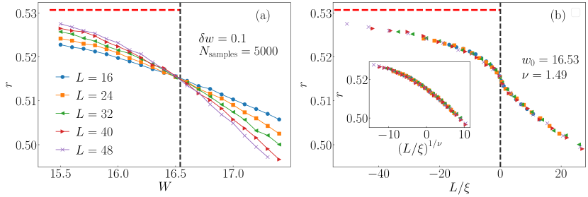
The distribution of again displays universal behaviour in accordance with its underlying level statistics [36, 37]. In the extended and localized regimes, the average is expected to converge towards the GOE and PE results, respectively [20, 37]. Tracing the change of the mean ratio from to allows one to distinguish the two regimes and perform a scaling analysis to obtain the critical parameter and scaling exponents. The quantity has only recently been employed in the studies of the 3D Anderson model [38] and is also the subject of the present paper. As an illustration, Figure 1 shows the results of the scaling analysis performed using the cost function minimization approach [19]. Using this method, we obtain the critical disorder value and an estimate for the critical exponent , which are in good agreement with the values reported elsewhere in the literature and given by Eq. (6). We discuss the method and the more technical details of our calculations in Sec. 4.
Going beyond the spectral correlations between consecutive levels, we briefly discuss the spectral form factor (SFF) [39, 16], to which we return in significantly more detail in Sec. 3.3. Much as the spectral statistics described above, the SFF also displays universal behaviour in the GOE and PE cases, however, its calculation also offers an insight into various time scales governing the dynamic behaviour of the studied systems. For instance, it allows for the determination of the Thouless time that denotes the time scale after which the quantum dynamics become universal and governed by the RMT. Introducing the Heisenberg time as the system’s longest physically relevant time scale, inversely proportional to the mean level spacing one can express the dimensionless logarithmic conductance as the logarithm of the ratio [17]
| (11) |
For simplicity, we refer to the logarithmic conductance as conductance throughout the work. It has recently been shown that requiring upon increasing the system size can be used as a very efficient tool for detection of the transition point in 3D and 5D Anderson models [18]. Furthermore, calculating the conductance as defined above, one can directly compare the results of a level statistics based approach with the results from level sensitivity statistics, such as the level curvatures. We study the latter in Sec. 3.1 and 3.2.
Finally, we note that the Anderson localization transition can also be studied through the structure of Hamiltonian eigenfunctions. Following the early works by Dean and Bell [40], this direction of research was pursued by many other authors (see, e.g., Ref. [25] for a review). Even though the eigenfunction properties are not the focus of this work, we briefly comment on the analysis of the eigenfunction fluctuations using the average inverse participation ratio (IPR). For an eigenstate , the IPR is defined as follows:
| (12) |
where is the normalized wave function written in the site-occupational basis and labels sites on the Hamiltonian’s underlying lattice. An analogous quantity is often investigated, namely the participation entropy :
| (13) |
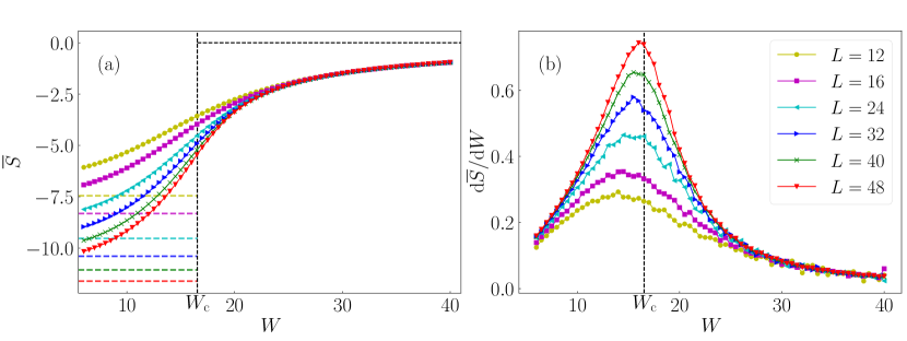
where the averages are defined analogously to those in Eq. (10). Plots of as a function of the disorder strength and system size are shown in Fig. 2(a).
In an ideally localized case, in which the probability density function equals unity on a single site and is zero elsewhere, it is immediately evident that and hence . This is the result at large in Fig. 2(a). In the opposite limit , the wave functions are uniformly spread over the lattice volume and hence the wave function coefficients are of the order . Consequently, in the thermodynamic limit the IPR vanishes as
with the disorder-dependent prefactor . In the absence of disorder, the wave functions are plane waves and hence while for weak disorder deep in the extended regime assumes its GOE value of 3. The corresponding results for in the former case are shown as horizontal dashed lines on the bottom of Fig. 2(a).
The numerical results presented in Fig. 2(a) are in agreement with the limiting cases discussed above. However, it is less clear how to extract a quantitative prediction for the localization transition from those results. Remarkably, as shown in Fig. 2(b), a very accurate estimate of the critical point can be obtained when studying the behavior of as a function of . It exhibits a peak at , where from Eq. (6) is shown by a vertical dashed line in Fig. 2(b). The results show that the peak becomes sharper with increasing the system size, moreover, its position gets closer to .
2.3 What is the main goal of this paper?
Having discussed some general features of the Anderson model, we now turn our attention to studies of some specific properties. The main goal of this paper is to contribute to a unified understanding of the localization transition in the 3D Anderson model using different spectrum based techniques. In Sec. 3 we contrast two widely used approaches, the first is based on the level sensitivity statistics and the second is based on the level statistics, to quantitatively pinpoint the transition point. In Sec. 4 we test the quality of the numerical scaling solution across the transition using a recently introduced method [19]. From the perspective of numerical calculations, we only report original results. That said, several quantities studied here were studied before by other authors using identical or slightly modified definitions. When applicable, we explicitly refer to those authors when discussing the results.
To obtain the energy spectra on which the subsequent analysis is performed, we employ the methods of exact numerical diagonalization. In Sec. 3, we use the method of full numerical diagonalization, since the knowledge of full spectra is needed for the calculation of quantities in question. To that end, we use the function eigvalsh from numpy.linalg Python library. Increased performance is achieved by using the version of numpy based on the Intel® Math Kernel Library. In Sec. 4, we turn to partial diagonalization approaches, since the quantities introduced only require a portion of the system’s eigenlevels for a successful calculation. To that end, we use the ‘shift-invert’ approach described in Ref. [41].
3 Indicators of localization transition: Level sensitivity statistics versus level statistics
We now proceed to the main part of this paper: the quantitative analysis of the determination of the critical point using two different approaches, i.e., the level sensitivity statistics and the level statistics. In the first approach reported in Secs. 3.1 and 3.2 we study the sensitivity of Hamiltonian eigenlevels to a change of boundary conditions. This approach was pioneered by Kohn in studies of ground state properties [42] and later generalized by Edwards and Thouless [8] to studies of arbitrary levels. In the second approach reported in Sec. 3.3 we use the spectral form factor to extract the characteristic time scales of the system.
3.1 Sensitivity to boundary conditions and level curvatures
To test the sensitivity of Hamiltonian eigenlevels towards the change of boundary conditions, we pierce the system by a flux along one of the axis (say, the -axis) with sites. The introduction of the flux modifies the kinetic energy term in the Anderson Hamiltonian, which is the first term in Eq. (1). In fact, the new operator only modifies the hopping along the -axis while other hopping terms remain unchanged. Its contribution along the -axis reads
| (14) |
where represents a double sum over all coordinates in the plane and . We refer to as . The sensitivity to boundary conditions is probed by considering a constant . This implies , and hence one can expand the Peierls phase in Eq. (14) up to the second order in , which yields
| (15) |
where we introduced the particle current operator . Using perturbation theory, the shift of the eigenlevels , expressed in the eigenbasis of the Anderson Hamiltonian in Eq. (1), is
| (16) |
For the real eigenstates considered here, . The central object we investigate is the level curvature , defined as
| (17) |
In particular, the quantity that we numerically calculate in this section to get is at .
Properties of the level curvatures as defined in Eq. (17) were subject of intense research in the past. Inspired by the work by Edwards and Thouless [8], perhaps the most widely studied property of is the width of its distribution (more precisely, the mean of its absolute value), which is related to the system’s conductivity via the Kubo-Greenwood formula [43]. This is going to be the main focus of our analysis below. We note that subsequent work also devoted considerable attention to other properties of . Examples include, e.g., the form of the distribution of [44, 45, 46] and the relation of level curvatures to other probes of level sensitivity such as the slopes of levels [47, 48, 49, 50, 46]. In a related development, the thermal average of was used as an indicator to distinguish quantum chaos from integrability in many-body systems [51], and the distribution of was studied in the random-field Heisenberg models [52, 53].
The main focus in the study of level curvatures by Edwards and Thouless was devoted to the structure of the sum in the parenthesis of Eq. (16). Under the assumption that its main contribution stems from a few nearest levels for which the current matrix elements are sufficiently uncorrelated with the corresponding level spacings, the contribution of the typical term can be estimated from the Kubo-Greenwood formula [43]. In other words, one can estimate the width of the level curvature distribution by a quantity that is proportional to the conductivity . In the diffusive regime, the dependence of the system size then only emerges through the term in Eq. (16), which results in . We note that using the Einstein relation one can also view the latter proportionality as , where is the diffusion constant.
In this work we numerically study the width of the level curvature distribution in the diffusive regime as well as across the localization transition. Specifically, we define the width of the curvature distribution as
| (18) |
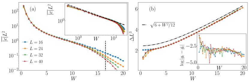
where denotes the arithmetic mean over 500 eigenstates around the center of the spectrum, and denotes the arithmetic mean over different disorder realizations for a given . As argued above, is expected to scale as in the diffusive regime. We verify this expectation in Fig. 3(a), where we plot the scaled curvature width . Indeed, the scaled results are -independent in a wide regime of disorders that, in finite systems, terminates close to the critical point at . The inset of Fig. 3(a) shows the results in a log-log scale. At small , the results are in agreement with the scaling , as predicted by perturbative arguments [54].
The results presented so far connect a particular property of level curvatures (specifically, the width of its distribution) to the conductivity . However, as discussed in Sec. 2, the central object in the scaling theory of localization is the conductance . These two quantities are in the diffusive regime related as , where is the system dimension. It is then suggested that one may define a conductance by multiplying the curvature width by a quantity that is proportional to . A natural candidate to achieve this is to divide it by the mean level spacing . The conductance defined in this way is sometimes referred to as the Thouless conductance.
While the precise definition of the conductance is going to be introduced below, we first discuss the definition of the mean level spacing . A convenient definition of is through the ratio of the energy width and the Hilbert space dimension , , where the Hilbert space dimension is in the three dimensional system and is a measure of the fraction of eigenstates (for a box distribution) in the interval between the mean energy and . In this way, can be calculated analytically since the energy variance of the entire single-particle space is in the thermodynamic limit given by
| (19) |
Nevertheless, since the curvature width is only averaged over the eigenstates in the center of the spectrum, we use an analogous definition to calculate the mean level spacing. We hence calculate the latter numerically as the arithmetic average over those levels that are also included in the calculation of in Eq. (18). We refer to it as , and the average over disorder realizations,
| (20) |
is also defined analogously to Eq. (18). Still, there is no substantial quantitative difference between and , as shown in the main panel of Fig. 3(b).
In the next step we define the conductance studied in this work. As argued above, it corresponds to the ratio of the curvature width and the mean level spacing. We define the conductance as a logarithm of this ratio to simplify its analysis for different regimes of disorder when it varies by several orders of magnitude. In general, one can apply several different protocols of the disorder averaging. Here we consider two such possibilities. The first is the disorder average of the ratio
| (21) |
and the second is the ratio of the disorder averages,
| (22) |
The inset in Fig. 3(b) shows that the differences between and are actually very small for essentially all disorder values we are interested in. We therefore proceed with studying from Eq. (21) in all further calculations. We attribute the origin of the numerical agreement between and to the fact that despite the average over eigenstates includes a considerable amount of eigenstates (500), this number is still small when compared to the total number of eigenstates. We note that 24 years ago, an analogous quantity was calculated by Braun, Hofstetter, MacKinnon and Montambaux for system volumes up to by averaging over roughly half of the spectrum [55].
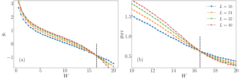
Figure 4 represents one of the main results of this work. In particular, Fig. 4(a) shows the conductance as defined in Eq. (21). In the diffusive regime at , when the curvature width scales as , the conductance increases as . On the other hand, in the localized regime at , the curvature width decreases even faster with than the mean level spacing, and hence decreases with increasing the system size. Results in Fig. 4(a) suggest that there exists a disorder value for which becomes independent of the system size. In fact, this disorder value is indeed very close to the critical disorder obtained by using other measures of the transition discussed in Sec. 2.
It is also remarkable that the results in Fig. 4(a) look very similar to the results in Fig. 4(b), in which we calculate another transition indicator, namely the conductance , which was introduced in Sec. 2.2. The latter is obtained from the level statistics analysis of the Hamiltonian without the flux. Further details about are discussed in Sec. 3.3.
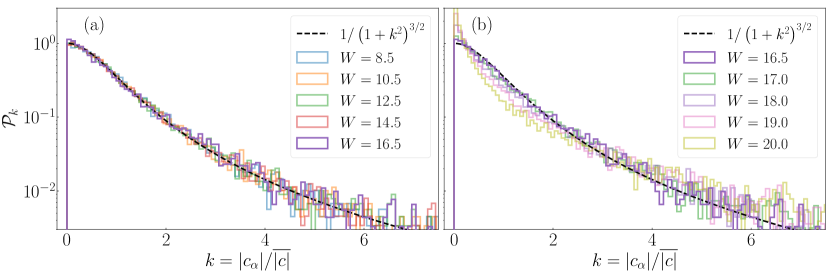
In addition to the studies of the mean level curvatures, Fig. 5 displays the properties of the level curvature distributions upon changing the disorder strength parameter. Once the level curvatures are rescaled by the mean level curvature , distributions in the delocalized regime exhibit universal properties [44, 45, 55]. First empirically guessed by Zakrzewski and Delande [44] and then analytically confirmed by von Oppen [45], the distribution of level curvatures is given by the expression
| (23) |
where is the normalizing constant with and in the GOE case with time-reversal symmetry (our interest here) and in the GUE case without time-reversal symmetry. Our numerical results in Fig. 5(a) for the largest system size available, , seem to confirm the validity of the universal prediction given by Eq. (23) up to the critical disorder strength . Deviations from the universal prediction become pronounced when the disorder is increased above , as shown in Fig. 5(b). The distributions in the localized regime develop a sharper peak at smaller curvatures and broader tails, consistent with previous studies (see, e.g., Ref. [55]).
3.2 Relation to the numerical implementation by Edwards and Thouless
We extend the previous section by making an explicit connection to the numerical implementation of the curvature calculation by Edwards and Thouless in their pioneering work [8]. They calculated the change of eigenenergies upon modifying the boundary conditions from periodic to antiperiodic at one lattice edge. Within the formalism in Sec. 3.1, this corresponds to the introduction of the flux along the -axis. We define the change of energy of an eigenlevel as
| (24) |
Then, we define the Edwards-Thouless (ET) energy as
| (25) |
where denotes the arithmetic mean over 500 eigenstates around the center of the spectrum, and denotes the arithmetic mean over different disorder realizations for a given . The definition of in Eq. (25) is, up to a normalization constant, analogous to the average over the absolute values of curvatures at defined in Eq. (18).
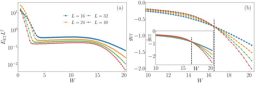
While Edwards and Thouless studied the Anderson model on a square lattice and a diamond lattice [8], we here implement an analogous numerical procedure for the cubic lattice. The first question that we address is the system size dependence of the Edwards-Thouless energy . For the width of the curvature distribution, Fig. 3(a) demonstrated that in the diffusive regime. In contrast, Fig. 6(a) shows that the scaled Edwards-Thouless energy is, for the system sizes under investigation, not a system size independent quantity. This may suggest that higher order terms in Eq. (16) may contribute to an additional system size dependence that is absent in the case when . This also precludes one to make an explicit connection between the scaled energy and the conductivity.
However, we show below that still represents a useful quantity to pinpoint the localization transition in finite systems. To this end we define the logarithm of the ratio of the Edwards-Thouless energy and the mean level spacing,
| (26) |
This quantity can be seen as the analog of the conductance from Eq. (21). Results for versus are shown in the main panel of Fig. 6(b). Their main feature is that the crossing point of , i.e., the disorder value at which becomes system size independent, is indeed very close to the critical disorder . In this spirit, one can apply to pinpoint the localization transition with similar numerical accuracy as compared to the conductances and shown in Fig. 4.
We finally comment on the impact of averaging over the system’s eigenstates. In all the numerical calculations so far we performed the arithmetic mean over eigenstates. We also tested the robustness of the results upon replacing the arithmetic mean with the geometric mean. We show an explicit example for in Eq. (26), in which the arithmetic mean is replaced by the geometric mean, yielding . Results for are shown in the inset of Fig. 6(b). They show that also in this case, the disorder value at which is independent of the system size is very close to the critical disorder obtained by other measures of the transition. Hence, these results suggest that the type of averaging does not lead to any significant quantitative difference with respect to the identification of the critical point. Similarly, we also observed (not shown) that the type of the disorder averaging does not have any significant impact on the scaling properties of presented in Fig. 3(a).
3.3 Spectral form factor
Results from the previous sections are now contrasted to the analysis based on spectral statistics of the Anderson Hamiltonian without the presence of a flux. The central quantity in the analysis is the spectral form factor (SFF), which is a Fourier transform of the spectral two-point correlations, defined as
| (27) |
In this expression, denote the complete ordered set of single-particle eigenvalues of after spectral unfolding. The unfolding procedure is initiated by defining the cumulative spectral function , where is the unit step function, followed by fitting a polynomial of degree 3 to . The unfolded eigenvalues are then defined as . We thereby set the local mean level spacing to unity at all energy densities, and we refer to the corresponding time in these units as the scaled time. In our analysis we consider properties of the Heisenberg time and the Thouless time. The Heisenberg time is defined as the inverse mean level spacing (times , which is set to unity), and the Thouless time is defined below. Since we are only interested in the ratio of those times, it is sufficient to consider them in their scaled units. As a consequence of the unfolding procedure, the scaled Heisenberg time is .
Note that in the definition of the SFF in Eq. (27), we included the Gaussian filter , which eliminates contributions from the spectral edges. The filtering function is defined as , where and are the mean energy and the variance, respectively, for a given disorder realization, and controls the effective fraction of eigenstates included in . The normalization then assures . Since the SFF is a not a self-averaging quantity [56], an additional averaging needs to be performed in order to obtain physically relevant results. As suggested in the literature [56], we use both ensemble and time averaging to reduce the fluctuations of the SFF. We perform the former by averaging our results over different disorder realizations at a given , which we denote by . Using a sufficiently narrow sliding window [56], we then perform the time averaging as well.
In physical systems that exhibit quantum chaos, the SFF is usually nonuniversal at short times, apart from the ultrashort time when (it is dominated by the density of states or the filter function ), which is not the focus of this work. Our main interest is the long time regime, in which becomes universal in the sense that it matches the prediction from the Gaussian orthogonal ensemble (GOE) of the RMT [16],
| (28) |
As a consequence, there exists a characteristic time which marks the crossover from a nonuniversal short time dynamics to the universal long time dynamics. This time is now denoted as the Thouless time in the literature, even though Thouless himself, as argued in Secs. 3.1 and 3.2, was primarily interested in the level sensitivity statistics rather than level statistics. Numerically, we determine the scaled Thouless time from the criterion , as described in [17]. We set to get the results for , which are shown in Figs. 4(b) and 7(a).
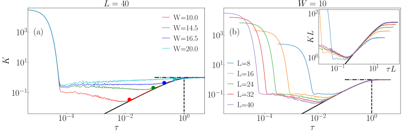
The single-particle spectrum of the 3D Anderson model below the localization transition is expected to comply with the GOE predictions [10, 11]. In the context of the SFF , this means that there exists a regime at in which , as discussed above. This is illustrated in Fig. 7(a) for a lattice with sites. Below the localization transition, i.e., at and 14.5 in Fig. 7(a), the results show that , denoted by circles, is much smaller than 1. In contrast, above the localization transition, i.e., at in Fig. 7(a), there is essentially no regime at in which , and hence our numerical analysis yields .
Some properties of the SFF in the 3D Anderson model have been recently studied by Sierant, Delande and Zakrzewski [18]. They showed that in the diffusive regime well below the critical point, the Thouless time in physical units scales with the linear system size as . We here corroborate this result with the analysis in Fig. 7(b) for the particular disorder value . The results in the main panel of Fig. 7(b) show a drift of the scaled Thouless time with increasing the system size, which suggests that the Thouless time in physical units scales slower than . In the inset of Fig. 7(b), we plot the scaled SFF as a function of . In this case the scaled Thouless time appears to be independent of the system size, which indicates that the Thouless time in physical units is proportional to . We also note that the authors of Ref. [18] also studied the Thouless time in physical units divided by the system volume, which is related to the conductance that we define below.
In Eq. (21) of Sec. 3.1 we introduced the conductance as an indicator of the localization transition based on the level sensitivity statistics. Here we introduce an analogous quantity (also termed conductance) based on the SFF analysis. In particular, the indicator of the transition is defined as the logarithm of the ratio of the Heisenberg and the Thouless time [17],
| (29) |
where the ratio has been expressed in terms of scaled times, and hence the scaled Heisenberg time can be set to unity. The definition of in Eq. (29) using the ratio of scaled times is identical to the one in Eq. (11) that uses the ratio of times in physical units. Results for the conductance as a function of are shown in Fig. 4(b). They share striking similarities with the conductance studied in Sec. 3.1. In particular, they both provide an efficient measure to pinpoint the transition point since in both cases the curves for different system sizes cross at the disorder value that is extremely close to the well-established critical disorder value discussed in Sec. 2.
To summarize our results for the scaling of conductances across the transition, they suggest that a very accurate estimate of the localization transition is obtained by requiring
| (30) |
where c, ET, or SFF [cf. Eqs. (21), (26) and (29), respectively]. This quantitative agreement signals a connection between the system’s sensitivity to boundary conditions and the validity of the underlying RMT description for unperturbed levels.
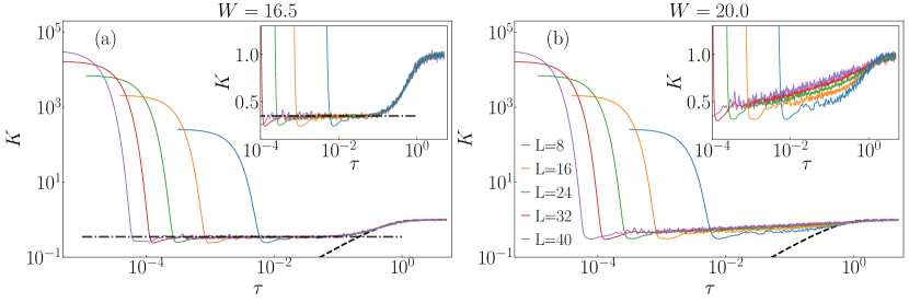
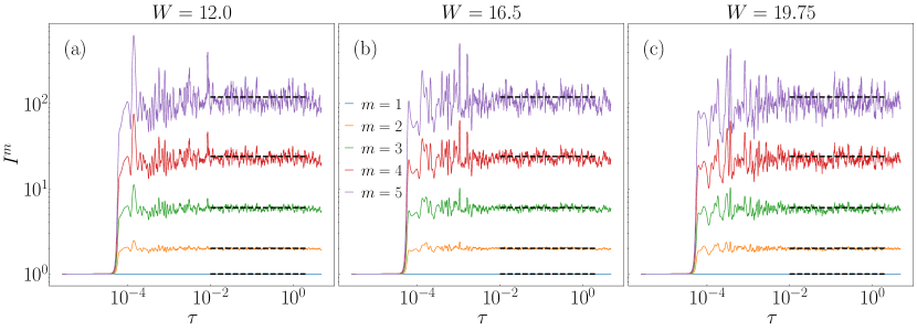
We next consider some further details of the SFF in the vicinity of the critical point. Equation (30) suggests that does not scale with the system size at the critical point . This is indeed consistent with the results in Fig. 8(a) for , which shows for different system sizes. Moreover, the results in Fig. 8(a) also suggest two related observations, which we discuss below.
The first observation is that . This suggests the emergence of a time interval , in which the SFF at the critical point matches the GOE prediction . Hence, within the framework of the SFF analysis introduced here, one may interpret the results as the Thouless time being smaller than the Heisenberg time at the localization transition.
The second observation is that the SFF at is, to a high numerical accuracy, independent of for several orders of magnitude. The value of in this regime is marked by a horizontal dashed-dotted line in Fig. 8(a). We note that in the localized regime at we do not observe a similar structure of , at least for the system sizes under investigation. This is illustrated for in Fig. 8(b). In particular, the inset of Fig. 8(b) shows a different finite-size trend of the results at when compared to those at the critical point. Results for at the critical point appear to be consistent with other measures of level statistics such as the level variance, which was shown to scale as at the critical point, where is the level compressibility [11, 57, 14, 58, 59, 60]. Indeed, if the latter expression holds true at all energy scales, it corresponds to a constant SFF , and can be traced back to multifractality of eigenfunctions [58]. The numerical value of the plateau height extracted from Fig. 8(a) is not far from the value obtained in the study of the level variance by Altshuler, Zharekeshev, Kotochigova and Shklovskii [11].
We conclude this section by a comment on the fluctuations of the SFF . We define higher moments of the as [61, 62]
| (31) |
and study the time-resolved ratio of the -th moment relative to the two-point SFF to the power ,
| (32) |
The main question that we address is the sensitivity of the fluctuation measure to the localization transition. An analytical estimate of in the localized phase can be obtained by assuming that the phases are i.i.d. complex random numbers with a vanishing mean and unit variance. Neglecting the filter function in Eq. (31), one observes that
| (33) |
where denotes the symmetry group of objects, which contains elements. As a consequence, the fluctuation measure in this approximation equals . Exactly the same result applies also in the standard RMT ensembles, e.g., the GOE [61].
Numerical results for are shown in Fig. 9 for three different disorder values which correspond to the disorder below, at and above the transition. The results appear to be very similar. In particular, the prediction , see the horizontal lines in Fig. 9, represents a good estimate for at small . While the agreement is expected for the GOE regime and the localized regime, we observe no qualitative change in behaviour at the localization transition. The temporal fluctuations of the SFF hence appear to be insensitive to the localization transition.
4 Scaling solutions across the transition
While the goal of the previous section was to compare different spectrum related methods to pinpoint the critical point, we here turn our attention to numerical scaling solutions of transition indicators across the localization transition. We first review some important steps of the conventional scaling analyses in Sec. 4.1. The advantage of those scaling analyses, studied extensively in the last decades [21, 63, 64, 65, 66, 67, 22, 38], is to provide information about the critical point, the critical exponents, and the corrections to scaling [21]. However, such procedure usually also requires the scaling functions to be expanded in power series in the vicinity of the critical point. In Sec. 4.2 we approach the problem from a different perspective. Disregarding our previous knowledge of the problem, we assume the precise location of the critical point in the 3D Anderson model is not known and hence the series expansion of the scaling functions cannot be applied. What other approaches could then be used in order to obtain meaningful information about the critical parameters? We show that the cost function minimization procedure with a floating crossing point [19] represents one of such tools. It allows for finding the optimal scaling collapse in the targeted parameter region without assuming any particular form of the scaling function, apart from the choice of the family of the correlation length functions. Moreover, it also allows for detecting the finite-size corrections to the critical point, which in the case of the 3D Anderson model share some similarities with the irrelevant scaling variables used in the context of conventional scaling analyses.
4.1 Scaling analysis using relevant and irrelevant scaling variables
Let us consider a dimensionless transition indicator , for which we apply the scaling analysis framework used by Slevin and Ohtsuki [21]. In their work represented a scaled correlation length, while here we refer to it as a general localization transition indicator. Then, building on the renormalization group arguments for the scaling behavior across the transition [68], is expected to behave in finite systems as
| (34) |
where represents some unknown function, and and are scaling variables. They are both functions of the scaled disorder, and , where and is the critical point. We refer to as a relevant scaling variable and is the dominant irrelevant scaling variable. The latter is irrelevant since we assume in Eq. (34), i.e., its contribution is negligible for large enough .
A standard assumption is that the irrelevant contribution is small and hence the function in Eq. (34) can be expanded in a power series around , yielding
| (35) |
where . Since in general none of the functions in Eq. (35) are known, it is convenient to expand them in a power series around the critical point,
| (36) |
where . Moreover, the scaling variables can also be expanded in power series, and . This leads in total to free fitting parameters. It is clear that such expansions are efficient if the critical point can be located to a sufficient accuracy without the scaling analysis. Indeed, this seems to be a reasonable assumption for the 3D Anderson model.
The usual choice made by the majority of works including ours, is that the relevant scaling variable is linear, . We hence set further on. Still, there are plenty of other options for the truncation of the series introduced above. For example, in the works by Slevin, Ohtsuki and collaborators, they tested robustness of critical parameters towards the choice of the cutoff parameters to describe the scaling properties of the dimensionless correlation length [21, 63, 22] and the wave function multifractality [66, 67]. Recently, Tarquini, Biroli and Tarzia [38] applied a similar scaling analysis using and to seek for the scaling collapse of the level spacing ratio from Eq. (10). The latter quantity is also going to be the focus of our analysis in the next section.
4.2 Scaling analysis using the cost function minimization with a floating crossing point
In contrast to the analysis in the previous section, there are many systems in which the critical point in the thermodynamic limit is not known to sufficient accuracy. In such case the low-order polynomial expansion of the scaling function, as expressed in Eqs. (35) and (36), may be inefficient.
The cost function minimization approach, introduced in [19] and applied in [17], is a numerical approach to find the optimal scaling collapse of a transition indicator as a function of , where is the correlation length. Let be a function of the disorder and system size . Then, we refer to the optimal scaling collapse as the one that minimizes the cost function ,
| (37) |
where denotes the number of all data points of included in the cost function minimization procedure, and denotes the value of at a given and . We sort all values of according to nondecreasing values of , where is referred to as the crossing point in finite systems that eventually converges to the critical point in the thermodynamic limit . Then, using a differential evolution method, we obtain the best data collapse by finding the fitting parameters for which the cost function is minimal. The cost function is defined such that the ideal data collapse yields , and otherwise.
One of the main advantages of the cost function approach is that it does not require any knowledge about the scaling function. Therefore, its application is not restricted to the data in the vicinity of the critical point, where the scaling function can be approximated using series expansion. Nevertheless, a convenient aspect of the conventional scaling analysis discussed in Sec. 4.1 is that it accounts for the drift of the crossing point in finite systems due to the presence of irrelevant scaling variables. We mimic this effect by allowing for the crossing point to be system size dependent, i.e., . The crossing point enters the scaling analysis through the linear scaling variable . We then denote the scaling variable as , and the scaling function can be written as
| (38) |
In this approach the optimal scaling solution may shift the curves at a fixed in the horizontal direction, but not in the vertical direction. Its application is therefore convenient when seeking for global scaling collapses of quantities that have well defined upper and lower values. We dub the method as the cost function minimization approach with a floating crossing point.
Below we test our approach using the level spacing ratio defined in Eq. (10). Its simplest application is shown in Fig. 1. The search of the numerical scaling solution is built on the preexisting knowledge of the location of the critical point, since the data included in the cost function minimization procedure correspond to a narrow symmetric interval around , i.e., . In this case, it is sufficient to consider the crossing point as a system independent parameter . Then, the function in Eq. (38) is a function of , where . Using the cost function minimization procedure we find the optimal values of two fitting parameters and , which are very close to the critical parameters given in Eq. (6).
In the remainder of the analysis we focus on two main goals. The first goal is to study the role of the target window for which the scaling solution is obtained. As discussed in Sec. 2.2 and demonstrated in Fig. 10(a), extends from the GOE regime below the transition with , to the Poisson regime above the transition with . The question that we address is: supposing that the entire crossover region of is included in the search of the scaling solution, can one still get an accurate estimate of the critical point? The second goal is to test how accurately the critical point can be estimated if one leaves the crossing point in finite systems to float with system size, i.e., the crossing point may be an arbitrary function of the system size. The use of such floating crossing point is very convenient if the accurate location of the critical point is not known and results in a wide disorder interval are included in the search of the scaling solution.
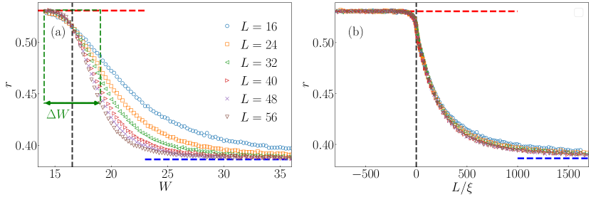
The rectangular frame in Fig. 10(a) is a sketch to mark the data which are included in the search of the optimal scaling solution. The width of the frame is denoted by . To obtain the scaling collapse in Fig. 10(b) we use as marked in Fig. 10(a), while the analysis in Fig. 11 is carried out as a function of varying . The scaling solution in Fig. 10(b) is obtained using an identical cost function minimization procedure as in Fig. 1(b) since in both cases there are two free fitting parameters, the crossing point and the critical exponent . However, since in Fig. 10 we use a larger than in Fig. 1, as well as a larger step between consecutive data points and less disorder averaging, the resulting optimal parameters (see figure captions for details) are slightly less accurate when compared to the values in Eq. (6).
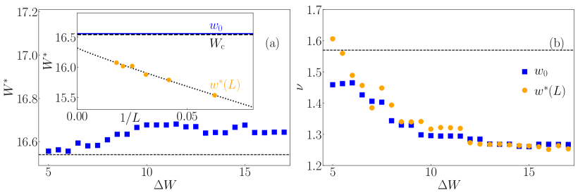
Next we increase and study how the critical parameters evolve as a function of . We first consider the simplest case where the crossing point is a system size independent number . We show versus in Fig. 11(a) and versus in Fig. 11(b). It is interesting to compare the results at relatively small (also used in Fig. 10) and at large . In the latter case the data included in the cost function minimization extend over almost the entire crossover region between and . We observe that the crossing point is determined very accurately even at . In contrast, the optimal value of deviates much stronger at larger . These results suggest a considerable robustness of the critical point towards the finite-size effects. This observation seems to be related to the fact that even numerical studies of the 3D Anderson model in the seventies and early eighties, using very limited computational resources, detected the critical properties with reasonable accuracy [69, 70, 71].
Finally we apply the cost function minimization procedure to the data in the rectangular frame in Fig. 10(a) using the free crossing point . In this case, the crossing point is an independent fitting parameter for each . Hence the total number of fitting parameters is seven (six parameters for six different system sizes, and the critical exponent ). The size dependent crossing point is shown in the inset of Fig. 11(a). It exhibits two important features. First, when extrapolated to , it agrees with the value of the critical point in Eq. (6) rather accurately. Second, we find a good fit for with , where . This is close to the recent study of the scaling properties of using the irrelevant scaling parameter , which reported [38]. We note, though, that the latter agreement is a mere observation since we are not aware of a theory predicting that and should be identical.
The results of this section suggest two convenient properties of the cost function minimization approach with a floating crossing point: it can be applied to systems in which the critical point is not yet known precisely, and it mimics to a certain extent the role of irrelevant scaling variables. For the specific example of the 3D Anderson model, the floating crossing point in finite system convincingly converged to the vicinity of the critical point predicted by other methods.
5 Conclusions
In this paper we discussed, compared and calculated several characteristic spectral features of the 3D Anderson model. While all those properties were to some extent already studied in the past, we considered them through the lens of modern numerical approaches and put an effort into making quantitative connections between them. The main focus was devoted into the comparison between the level sensitivity statistics and the level statistics. Specifically, we compared the width of the level curvatures distribution and the Thouless time extracted from the spectral form factor. We showed that, using proper normalization, both quantities behave very similarly and provide an efficient tool to pinpoint the localization transition. We then also made a quantitative connection of those quantities to the quantities studied in the work by Edwards and Thouless [8]. Finally, we study the numerical scaling solutions of the level spacing ratio in the vicinity of the critical point. We showed that the cost function minimization approach with a floating crossing point [19] provides a framework to accurately pinpoint the critical point. Moreover, it provides an additional information about the finite-size corrections that to certain extent resemble the behavior of irrelevant scaling variables used in the conventional scaling analysis.
6 Acknowledgments
We acknowledge insightful discussions with P. Prelovšek. This work was supported by the Slovenian Research Agency (ARRS), Research Core Fundings Grants No. P1-0044, No. P1-0402 and No. J1-1696, and by European Research Council (ERC) under Advanced Grant 694544 – OMNES.
References
- [1] P. W. Anderson, Absence of diffusion in certain random lattices, Phys. Rev. 109 (1958) 1492–1505. doi:10.1103/PhysRev.109.1492.
- [2] B. Kramer, A. MacKinnon, Localization: theory and experiment, Rep. Prog. Phys. 56 (12) (1993) 1469–1564. doi:10.1088/0034-4885/56/12/001.
- [3] A. Lagendijk, B. Van Tiggelen, D. S. Wiersma, Fifty years of Anderson localization, Physics Today 62 (8) (2009) 24–29. doi:10.1063/1.3206091.
- [4] N. F. Mott, W. D. Twose, The theory of impurity conduction, Advances in Physics 10 (38) (1961) 107–163. doi:10.1080/00018736100101271.
- [5] R.E. Borland, The nature of the electronic states in disordered one-dimensional systems, Proceedings of the Royal Society of London. Series A. Mathematical and Physical Sciences 274 (1359) (1963) 529–545. doi:10.1098/rspa.1963.0148.
- [6] N. F. Mott, Conduction in glasses containing transition metal ions, Journal of Non-Crystalline Solids 1 (1) (1968) 1–17. doi:10.1016/0022-3093(68)90002-1.
- [7] E. Abrahams, P. W. Anderson, D. C. Licciardello, T. V. Ramakrishnan, Scaling theory of localization: Absence of quantum diffusion in two dimensions, Physical Review Letters 42 (10) (1979) 673–676. doi:10.1103/PhysRevLett.42.673.
- [8] J. T. Edwards, D. J. Thouless, Numerical studies of localization in disordered systems, J. Phys. C 5 (1972) 807. doi:10.1088/0022-3719/5/8/007.
- [9] D. J. Thouless, Electrons in disordered systems and the theory of localization, Physics Reports 13 (3) (1974) 93–142. doi:10.1016/0370-1573(74)90029-5.
- [10] B. Al’tshuler, B. Shklovskii, Repulsion of energy levels and conductivity of small metal sample, Zh. Eksp. Teor. Fiz. 91 (1986) 220.
- [11] B. Al’tshuler, I. Zharekeshev, S. Kotochigova, B. Shklovskii, Repulsion between energy levels and the metal-insulator transition, Zh. Eksp. Teor. Fiz. 94 (1988) 343.
- [12] B. I. Shklovskii, B. Shapiro, B. R. Sears, P. Lambrianides, H. B. Shore, Statistics of spectra of disordered systems near the metal-insulator transition, Phys. Rev. B 47 (1993) 11487–11490. doi:10.1103/PhysRevB.47.11487.
- [13] E. Hofstetter, M. Schreiber, Statistical properties of the eigenvalue spectrum of the three-dimensional Anderson Hamiltonian, Phys. Rev. B 48 (1993) 16979–16985. doi:10.1103/PhysRevB.48.16979.
- [14] I. K. Zharekeshev, B. Kramer, Scaling of level statistics at the disorder-induced metal-insulator transition, Phys. Rev. B 51 (1995) 17239–17242. doi:10.1103/PhysRevB.51.17239.
- [15] I. K. Zharekeshev, B. Kramer, Asymptotics of universal probability of neighboring level spacings at the Anderson transition, Phys. Rev. Lett. 79 (1997) 717–720. doi:10.1103/PhysRevLett.79.717.
- [16] M. L. Mehta, Random Matrices and the Statistical Theory of Spectra, 2nd ed., Academic, New York, 1991.
- [17] J. Šuntajs, J. Bonča, T. Prosen, L. Vidmar, Quantum chaos challenges many-body localization, Phys. Rev. E 102 (2020) 062144. doi:10.1103/PhysRevE.102.062144.
- [18] P. Sierant, D. Delande, J. Zakrzewski, Thouless Time Analysis of Anderson and Many-Body Localization Transitions, Phys. Rev. Lett. 124 (2020) 186601. doi:10.1103/PhysRevLett.124.186601.
- [19] J. Šuntajs, J. Bonča, T. Prosen, L. Vidmar, Ergodicity breaking transition in finite disordered spin chains, Phys. Rev. B 102 (2020) 064207. doi:10.1103/PhysRevB.102.064207.
- [20] V. Oganesyan, D. A. Huse, Localization of interacting fermions at high temperature, Phys. Rev. B 75 (15) (2007) 1–5. arXiv:0610854, doi:10.1103/PhysRevB.75.155111.
- [21] K. Slevin, T. Ohtsuki, Corrections to Scaling at the Anderson Transition, Phys. Rev. Lett. 82 (1999) 382–385. doi:10.1103/PhysRevLett.82.382.
- [22] K. Slevin, T. Ohtsuki, Critical exponent for the anderson transition in the three-dimensional orthogonal universality class, New J. Phys. 16 (1) (2014) 015012. doi:10.1088/1367-2630/16/1/015012.
- [23] K. Slevin, T. Ohtsuki, Critical exponent of the Anderson transition using massively parallel supercomputing, J. Phys. Soc. Jpn. 87 (9) (2018) 094703. doi:10.7566/JPSJ.87.094703.
- [24] P. A. Lee, T. V. Ramakrishnan, Disordered electronic systems, Rev. Mod. Phys. 57 (2) (1985) 287–337. doi:10.1103/RevModPhys.57.287.
- [25] F. Evers, A. D. Mirlin, Anderson transitions, Rev. Mod. Phys. 80 (2008) 1355–1417. doi:10.1103/RevModPhys.80.1355.
- [26] P. Markoš, Numerical analysis of the Anderson localization, Acta Physica Slovaca 56 (2006) 561. doi:10.2478/v10155-010-0081-0.
- [27] A. MacKinnon, B. Kramer, One-parameter scaling of localization length and conductance in disordered systems, Phys. Rev. Lett. 47 (1981) 1546–1549. doi:10.1103/PhysRevLett.47.1546.
- [28] A. MacKinnon, B. Kramer, The scaling theory of electrons in disordered solids: Additional numerical results, Zeitschrift für Physik B Condensed Matter 53 (1) (1983) 1–13. doi:10.1007/BF01578242.
- [29] J. L. Pichard, G. Sarma, Finite size scaling approach to Anderson localisation, J. Phys. C 14 (6) (1981) L127–L132. doi:10.1088/0022-3719/14/6/003.
- [30] J. L. Pichard, G. Sarma, Finite-size scaling approach to Anderson localisation. II. Quantitative analysis and new results, J. Phys. C 14 (21) (1981) L617–L625. doi:10.1088/0022-3719/14/21/004.
- [31] B. Kramer, K. Broderix, A. Mackinnon, M. Schreiber, The Anderson transition: New numerical results for the critical exponents, Physica A: Statistical Mechanics and its Applications 167 (1) (1990) 163–174. doi:10.1016/0378-4371(90)90050-3.
- [32] A. MacKinnon, Critical exponents for the metal-insulator transition, J. Phys.: Cond. Matt. 6 (13) (1994) 2511–2518. doi:10.1088/0953-8984/6/13/012.
- [33] M. Schreiber, H. Grussbach, Dimensionality dependence of the metal-insulator transition in the anderson model of localization, Physical Review Letters 76 (10) (1996) 1687–1690. doi:10.1103/PhysRevLett.76.1687.
- [34] I. Varga, E. Hofstetter, M. Schreiber, J. Pipek, Shape analysis of the level-spacing distribution around the metal-insulator transition in the three-dimensional Anderson model, Physical Review B 52 (11) (1995) 7783–7786. doi:10.1103/PhysRevB.52.7783.
- [35] I. K. Zharekeshev, B. Kramer, Critical level statistics at the Anderson transition in four-dimensional disordered systems, Annalen der Physik (Leipzig) 7 (5-6) (1998) 442–451. doi:10.1002/(SICI)1521-3889(199811)7:5/6<442::AID-ANDP442>3.0.CO;2-D.
- [36] P. Łydżba, M. Rigol, L. Vidmar, Entanglement in many-body eigenstates of quantum-chaotic quadratic Hamiltonians, Phys. Rev. B 103 (2021) 104206. doi:10.1103/PhysRevB.103.104206.
- [37] Y. Y. Atas, E. Bogomolny, O. Giraud, G. Roux, Distribution of the ratio of consecutive level spacings in random matrix ensembles, Physical Review Letters 110 (8). arXiv:1212.5611, doi:10.1103/PhysRevLett.110.084101.
- [38] E. Tarquini, G. Biroli, M. Tarzia, Critical properties of the Anderson localization transition and the high-dimensional limit, Physical Review B 95 (9) (2017) 94204. arXiv:1612.04753, doi:10.1103/PhysRevB.95.094204.
- [39] M. V. Berry, Semiclassical theory of spectral rigidity, Proc. R. Soc. Lond. A 400 (1819) (1985) 229. doi:10.1098/rspa.1985.0078.
-
[40]
R. J. Bell, P. Dean, Atomic
vibrations in vitreous silica, Discussions of the Faraday Society 50 (1970)
55–61.
doi:10.1039/DF9705000055.
URL http://xlink.rsc.org/?DOI=df9705000055 - [41] F. Pietracaprina, N. Macé, D. J. Luitz, F. Alet, Shift-invert diagonalization of large many-body localizing spin chains, SciPost Phys. 5 (5) (2018) 45. doi:10.21468/SciPostPhys.5.5.045.
- [42] W. Kohn, Theory of the insulating state, Phys. Rev. 133 (1964) A171–A181. doi:10.1103/PhysRev.133.A171.
- [43] N. F. Mott, Conduction in non-crystalline systems. IV. Anderson localization in a disordered lattice, The Philosophical Magazine: A Journal of Theoretical Experimental and Applied Physics 22 (175) (1970) 7–29. doi:10.1080/14786437008228147.
- [44] J. Zakrzewski, D. Delande, Parametric motion of energy levels in quantum chaotic systems. I. Curvature distributions, Phys. Rev. E 47 (1993) 1650–1664. doi:10.1103/PhysRevE.47.1650.
- [45] F. von Oppen, Exact distribution of eigenvalue curvatures of chaotic quantum systems, Phys. Rev. Lett. 73 (1994) 798–801. doi:10.1103/PhysRevLett.73.798.
- [46] Y. V. Fyodorov, H.-J. Sommers, ”Level curvature” distribution for diffusive Aharonov-Bohm systems: Analytical results, Phys. Rev. E 51 (1995) R2719–R2722. doi:10.1103/PhysRevE.51.R2719.
- [47] M. Wilkinson, Statistical aspects of dissipation by landau-zener transitions, J. Phys. A. 21 (21) (1988) 4021–4037. doi:10.1088/0305-4470/21/21/011.
- [48] E. Akkermans, G. Montambaux, Conductance and statistical properties of metallic spectra, Phys. Rev. Lett. 68 (1992) 642–645. doi:10.1103/PhysRevLett.68.642.
- [49] B. D. Simons, B. L. Altshuler, Universalities in the spectra of disordered and chaotic systems, Phys. Rev. B 48 (1993) 5422–5438. doi:10.1103/PhysRevB.48.5422.
- [50] D. Braun, G. Montambaux, Universal spectral correlations in diffusive quantum systems, Phys. Rev. B 50 (1994) 7776–7785. doi:10.1103/PhysRevB.50.7776.
- [51] H. Castella, X. Zotos, P. Prelovšek, Integrability and ideal conductance at finite temperatures, Phys. Rev. Lett. 74 (1995) 972–975. doi:10.1103/PhysRevLett.74.972.
- [52] M. Filippone, P. W. Brouwer, J. Eisert, F. von Oppen, Drude weight fluctuations in many-body localized systems, Phys. Rev. B 94 (2016) 201112. doi:10.1103/PhysRevB.94.201112.
- [53] A. Maksymov, P. Sierant, J. Zakrzewski, Energy level dynamics across the many-body localization transition, Phys. Rev. B 99 (2019) 224202. doi:10.1103/PhysRevB.99.224202.
- [54] G. Montambaux, H. Bouchiat, D. Sigeti, R. Friesner, Persistent currents in mesoscopic metallic rings: Ensemble average, Phys. Rev. B 42 (1990) 7647–7650. doi:10.1103/PhysRevB.42.7647.
- [55] D. Braun, E. Hofstetter, A. MacKinnon, G. Montambaux, Level curvatures and conductances: A numerical study of the Thouless relation, Phys. Rev. B 55 (1997) 7557–7564. doi:10.1103/PhysRevB.55.7557.
- [56] J. Cotler, N. Hunter-Jones, J. Liu, B. Yoshida, Chaos, complexity, and random matrices, Journal of High Energy Physics 2017 (11) (2017) 48. arXiv:1706.05400, doi:10.1007/JHEP11(2017)048.
- [57] D. Braun, G. Montambaux, Spectral correlations from the metal to the mobility edge, Phys. Rev. B 52 (1995) 13903–13909. doi:10.1103/PhysRevB.52.13903.
- [58] J. T. Chalker, V. E. Kravtsov, I. V. Lerner, Spectral rigidity and eigenfunction correlations at the Anderson transition, Jetp Lett. 64, (1996) 386. doi:10.1134/1.567208.
- [59] D. Braun, G. Montambaux, M. Pascaud, Boundary conditions at the mobility edge, Phys. Rev. Lett. 81 (1998) 1062–1065. doi:10.1103/PhysRevLett.81.1062.
- [60] M. L. Ndawana, R. A. Römer, M. Schreiber, Finite-size scaling of the level compressibility at the Anderson transition, Eur. Phys. J. B 27 (2002) 399. doi:10.1140/epjb/e2002-00171-4.
- [61] A. Flack, B. Bertini, T. Prosen, Statistics of the spectral form factor in the self-dual kicked Ising model, Phys. Rev. Research 2 (2020) 043403. doi:10.1103/PhysRevResearch.2.043403.
- [62] A. Chan, A. De Luca, J. T. Chalker, Spectral Lyapunov exponents in chaotic and localized many-body quantum systems, arXiv:2012.05295.
- [63] K. Slevin, T. Ohtsuki, T. Kawarabayashi, Topology dependent quantities at the Anderson transition, Phys. Rev. Lett. 84 (2000) 3915–3918. doi:10.1103/PhysRevLett.84.3915.
- [64] F. Milde, R. A. Römer, M. Schreiber, V. Uski, Critical properties of the metal-insulator transition in anisotropic systems, Eur. Phys. J. B. 15 (2000) 685. doi:10.1007/s100510051173.
- [65] K. Slevin, P. Markoš, T. Ohtsuki, Reconciling conductance fluctuations and the scaling theory of localization, Phys. Rev. Lett. 86 (2001) 3594–3597. doi:10.1103/PhysRevLett.86.3594.
- [66] A. Rodriguez, L. J. Vasquez, K. Slevin, R. A. Römer, Critical parameters from a generalized multifractal analysis at the Anderson transition, Phys. Rev. Lett. 105 (2010) 046403. doi:10.1103/PhysRevLett.105.046403.
- [67] A. Rodriguez, L. J. Vasquez, K. Slevin, R. A. Römer, Multifractal finite-size scaling and universality at the Anderson transition, Phys. Rev. B 84 (2011) 134209. doi:10.1103/PhysRevB.84.134209.
- [68] J. Cardy, Scaling and Renormalization in Statistical Physics, chap. 3, Cambridge University Press, Cambridge, 1996.
- [69] P. Prelovšek, Numerical simulation of diffusion in a three-dimensional disordered lattice, Solid State Communications 31 (3) (1979) 179–182. doi:https://doi.org/10.1016/0038-1098(79)90430-7.
- [70] D. Weaire, B. Kramer, Numerical methods for electronic properties of disordered solids, Journal of Non-Crystalline Solids 35-36 (1980) 9–14. doi:https://doi.org/10.1016/0022-3093(80)90565-7.
- [71] D. W. B. Kramer, A. MacKinnon, Numerical study of conductivity for the Anderson model in two and three dimensions, Phys. Rev. B 23 (12) (1981) 6357–6370.