Thermal Trigger for Solar Flares I: Fragmentation of the Preflare Current Layer

1 Introduction

sec1

In recent decades, space observatories have made it possible to study the development of solar flares in all the ranges of the electromagnetic radiation (Benz, 2017). The brightness of flare coronal loops in the ultraviolet range is one of the most spectacular manifestations of a solar flare which has been observed in detail. The complex structure of the distribution of bright loops in space indicates the heterogeneity of the primary energy release in a flare (Krucker, Hurford, and Lin, 2003; Reva et al., 2015). Nevertheless, quasiperiodicity in the spatial distribution of bright loops in a flare arcade can often be noticed. The Bastille day flare is a telling example of a well-observed flare arcade extending over the photospheric neutral line (Aulanier et al., 2000; Somov et al., 2002).

According to current understanding, a thin current layer is formed over the arcade of magnetic loops before the flare (Priest and Forbes, 2002; Somov, 2013; Toriumi and Wang, 2019). This current layer separates colliding magnetic fluxes preventing them to reconnect. This leads to the accumulation of free energy in a non-potential magnetic field associated with the current. Free energy is released in the form of a solar flare during fast magnetic reconnection when the preflare current layer is destroyed (Oreshina and Somov, 1998; Somov and Oreshina, 2000; Uzdensky, 2007). The aim of this work is to search for a mechanism that can lead to the destruction of the current layer that is quasiperiodic in space.

The effect of the decay of the current layer into individual current filaments is known as tearing instability (Furth, Killeen, and Rosenbluth, 1963; Somov and Verneta, 1993). This process separates the current layer along streamlines facilitating the transition from slow reconnection to fast one. However, it does not allow to see in which places along the current direction one should expect an increased energy release. The current layer decays entirely in the classical tearing instability. From the mathematical point of view, this is due to the absence of a wave-type solution in the direction along the current. Often, a similar solution was sought in the interaction of the current layer with magnetohydrodynamic (MHD) waves (Vorpahl, 1976; Nakariakov et al., 2006; Artemyev and Zimovets, 2012). Also, a spatially inhomogeneous energy release was considered as a result of the corrugation instability of a coronal arcade (Klimushkin et al., 2017). The magnetic field frozen into the plasma displaced by the instability could reconnect with the overlying magnetic field, leading to the heating of the unstable flux tube.

In Somov and Syrovatskii (1982), the heat balance inside the current layer (Syrovatskii, 1976) is considered. In fact, a particular case of thermal instability (Field, 1965) in the geometry of the current layer is studied. Investigation of the heat balance in the coronal plasma is applied in modeling the observed properties of magnetic loops (Klimchuk, 2019; Antolin, 2020) and prominences (Carbonell et al., 2006). Thermal imbalance leads to the unstable growth of entropy waves (Somov, Dzhalilov, and Staude, 2007) affecting the stability of magnetosonic waves (Claes and Keppens, 2019; Perelomova, 2020) and causing the dispersion of slow MHD waves (Zavershinskii et al., 2019). The heat-induced attenuation of slow waves in the cylindrical geometry of a magnetic tube (Nakariakov et al., 2017) is used to diagnose the plasma in coronal loops on the Sun (Kolotkov, Nakariakov, and Zavershinskii, 2019).

We consider a piecewise homogeneous model of a current layer, which consists of a magnetically neutral current layer surrounded by a plasma with an external magnetic field. In the equilibrium state, the plasma inside the current layer does not contain a magnetic field. However, the disturbance of the external magnetic field can penetrate inward when the screening currents are disturbed. The situation of the appearance of a magnetic field in an MHD medium that does not initially contain one is realized. This situation is interesting in itself, and not only in the context of magnetic reconnection. Therefore, we first consider the more general problem of the heat balance of a homogeneous plasma without a magnetic field (Section sec2). Then we apply the found solution to the particular geometry of the preflare current layer (Section sec3). Finally, we consider this current layer in the context of a coronal plasma (Section sec4). Our conclusions are given in Section sec5.

2 Thermal Instability of a Homogeneous Plasma

sec2

In order to study the physical nature of the process of instability formation, homogeneous plasma in the single-fluid dissipative MHD approximation is considered. The MHD approximation has been successfully used for coronal applications for more than 50 years (e.g. Nakariakov and Kolotkov, 2020). It imposes some restrictions on the possible plasma processes under consideration. First, these processes must be sufficiently slow compared with the time of electron-ion collisions, so that the Maxwell distribution of electrons and ions with a common temperature is established in the plasma. Plasma processes must be also sufficiently slow with respect to the inverse plasma conductivity to neglect the displacement current in comparison with conductive current in Maxwell’s equations. Second, the magnetic field must be weak enough to use isotropic conductivity in the generalized Ohm’s law. Third, the velocities of the considered plasma motions must be sufficiently small in comparison with the speed of light so that the action of electric forces as compared with magnetic ones can be neglected in the nonrelativistic limit.

The first condition satisfies our consideration of the preflare state of the plasma in the solar corona, when fast energy release does not yet take place, and the separation of electron and ion temperatures is not important. The second condition is consistent with the general idea of a solar flare as a result of the process of magnetic reconnection at the zero point of the magnetic field. The third condition is certainly valid in the context of the observed preflare plasma velocities in the solar corona. However, the effects of finite conductivity during the formation of the preflare current layer cannot be neglected. The subject of this study is the thermal balance of the plasma in the preflare configuration, and therefore it is assumed that Joule and viscous heating, thermal conductivity, and radiative cooling in the energy equation are preserved. Thus, the following set of dissipative MHD equations is sufficient for our consideration (Syrovatskii, 1958; Somov, 2012):

$$\frac{\partial n}{\partial t}+\mathrm{div}\,(n{\mathbfit v})=0\,,$$

$$\mu n\,\frac{\rm{d}{\mathbfit v}}{{\rm d}t}=-{\bf\nabla}(2nk_{{}_{\rm B}}T)-\frac{1}{4\pi}\,({\mathbfit B}\times\mathrm{curl}{\mathbfit B})+\eta\,\Delta{\mathbfit v}+\nu\,{\bf\nabla}\,\mathrm{div}\,{\mathbfit v}\,,$$

$$\frac{2nk_{{}_{\rm B}}}{\gamma-1}\,\frac{{\rm d}T}{{\rm d}t}-2k_{{}_{\rm B}}T\,\frac{{\rm d}n}{{\rm d}t}\\ =\frac{c^{2}}{(4\pi)^{2}\sigma}\,({\mathrm{curl}}{{\mathbfit B}})^{2}+\frac{\partial}{\partial r_{\alpha}}(\sigma_{\alpha\beta}v_{\beta})+{\mathrm{div}}\,(\kappa{\bf\nabla}T)-\lambda\,(n,T)\,,$$

$$\frac{\partial{{\mathbfit B}}}{\partial t}={\mathrm{curl}}\,({{\mathbfit v}}\times{{\mathbfit B}})-\frac{c^{2}}{4\pi}\,{\mathrm{curl}}\left(\frac{1}{\sigma}\,{\mathrm{curl}}{{\mathbfit B}}\right),$$

$${\mathrm{div}}{{\mathbfit B}}=0\,.\ilabel{01}$$ (1)

Here, $\mu=1.44\,m_{H}$, $m_{H}$ is the mass of the hydrogen atom, $k_{{}_{\rm B}}$ is the Boltzmann constant, $\gamma$ is the heat capacity ratio, $\kappa$ and $\sigma$ are the thermal and electric conductivities of the plasma, $\lambda\,(n,T)$ is the radiative cooling function, $\eta$ and $\nu$ are viscosity ratios, and $\sigma_{\alpha\beta}$ is the viscous stress tensor. Transfer coefficients are isotropic in the absence of an external magnetic field. The heat capacity ratio is assumed $\gamma=5/3$ for simplicity. $T$ is the temperature, $n$ is the palsma density, $v$ is the plasma velocity, and $B$ is the magnetic field. System (01) will be also used to describe a piecewise homogeneous model of the current layer in Section sec3.

2.1 Increments of Instability

sec2.1

The solution to Equations 01 in the form of the sum of a constant homogeneous term and a small perturbation is sought using the following Fourier transform with subsequent linearization in $f^{\prime}$

$$f({{\mathbfit r}},t)=f_{const}+f^{\prime}\,{\rm exp}\,(-i\omega t+i({\mathbfit k}{\mathbfit r}))\,.$$

Here $f^{\prime}\equiv\{{{\mathbfit v}^{\prime}},n^{\prime},T^{\prime},{{\mathbfit B}^{\prime}}\}$ are perturbation amplitudes.

Let us set ${{\mathbfit v}}_{\rm const}=0$ and ${{\mathbfit B}}_{\rm const}=0$. It is worth noting that both Joule and viscous heating turn out to be of second order in the perturbation and can be neglected in a linear phase. Only radiative cooling and thermal conductivity affect the thermal balance of the plasma in a linear approximation. The first seeks to cool the plasma, while the second redistributes heat between regions with different temperatures. Thus, the plasma tends to cool against the background of small perturbations. Naturally, this does not contradict the initial heat balance. Even if radiative cooling is not compensated by Joule or viscous heating in an unperturbed plasma, one can consider additional constant heating as part of the thermal function $\lambda$. An additional constant term creates an initial heat balance and does not affect small perturbations, since it disappears during the linearization (Hood, 1992; De Moortel and Hood, 2004; Claes and Keppens, 2019). It is also possible to consider a more general non-constant thermal function, but such a consideration goes beyond the physical formulation of our problem (Rosner, Tucker, and Vaiana, 1978; Ibanez S. and Escalona T., 1993; Kolotkov, Duckenfield, and Nakariakov, 2020). The set of linear equations will take the following form:

$$\omega\,n^{\prime}=n\,{({\mathbfit k}{\mathbfit v}^{\prime})}\,,\ilabel{02}$$ (2)

$$i\omega\,n\,{{\mathbfit v}}^{\prime}=i{{\mathbfit k}}\,\frac{2k_{{}_{\rm B}}}{\mu}\,(nT^{\prime}+Tn^{\prime})+k^{2}\,\eta\,{{\mathbfit v}}^{\prime}+\omega{{\mathbfit k}}\,\frac{\nu}{n}\,n^{\prime}\,,\ilabel{03}$$ (3)

$$i\omega\,\frac{2nk_{{}_{\rm B}}}{\gamma-1}\,T^{\prime}-i\omega\,2k_{{}_{\rm B}}T\,n^{\prime}=k^{2}\,\kappa\,T^{\prime}+\frac{\partial\lambda}{\partial T}\,T^{\prime}+\frac{\partial\lambda}{\partial n}\,n^{\prime}\,,\ilabel{04}$$ (4)

$$i\omega\,{{\mathbfit B}}^{\prime}=\frac{c^{2}}{4\pi\sigma}\,(k^{2}\,{{\mathbfit B}}^{\prime}-{{\mathbfit k}}\,({{\mathbfit k}{\mathbfit B}^{\prime}}))\,,\ilabel{05}$$ (5)

$$({{\mathbfit k}{\mathbfit B}^{\prime}})=0\,.\ilabel{06}$$ (6)

Equations 02 – 06 split into two subsystems of equations. The perturbations of velocity, concentration, and temperature enter only in the first three equations, while the perturbation of the magnetic field enters only in Equations 05 and 06. In this regard, it is worth paying attention to a couple of nuances.

First, we assume that ${\mathbfit B}^{\prime}\neq 0$. In this article, we will not investigate the reasons for the occurrence of a nonzero magnetic field perturbation in an initially magnetically neutral plasma. Such a study goes beyond the framework of our MHD approach and requires the use of kinetic theory, such as the Weibel instability (Weibel, 1959). In this section, we want to show that the formation of a magnetic field perturbation creates a dedicated frequency in a broadband disturbance subject to thermal instability. In what follows, when considering the piecewise homogeneous model of the preflare current layer (Section sec3), we will assume that the perturbation of the magnetic field penetrates into the magnetically neutral current layer from the surrounding plasma upon dissipation of the screening currents flowing over the surface of the current layer in an unperturbed state. The formulation of the problem implies the appearance of a magnetic field in a medium that initially does not contain one, and this is exactly what we expect in the region of magnetic reconnection. External magnetic fields compensate each other inside the current layer in equilibrium state, but they can penetrate inside when electric currents are disturbed.

Second, the division of the Equations 01 into subsystems of equations does not indicate the formation of several perturbation modes, as is the case in a complete MHD system with a magnetic field during the formation of entropy, Alfvén, and slow and fast magnetoacoustic waves. Mode separation occurs when one dispersion relation allows several different solutions, but here we have several dispersion relations for one solution. It is also not a resonance between different solutions, because we are initially looking for one solution that satisfies two conditions. The system of Equations 02 – 04 describes the linear evolution of entropy and sound modes in a nonideal hydrodynamic medium, but Equations 05 and 06 additionally require the occurrence of a magnetic field perturbation. This disturbance should not be confused with standard fast and slow magnetoacosutic waves for which the existence of the initial guiding field is essential. The system of Equations 02 – 06 describes a hydrodynamic disturbance that allows a magnetic field to arise. This type of perturbations requires specific conditions that occur in coronal plasma structures such as current layers only.

Two different subsystems allow us to directly determine the frequency of perturbations which may become unstable according to the scenario described above. Let us substitute Equation 06 in Equation 05 and express the value of $k^{2}$. Then we multiply Equation 03 per the wave vector ${\mathbfit k}$ and replace $({\mathbfit k}{\mathbfit v}^{\prime})$ and $k^{2}$ by Equations 02 and 05, respectively. Finally, we exclude one of the perturbations $n^{\prime}$ and $T^{\prime}$ from Equation 03 with the help of Equation 04. Then the second perturbation is absent in the resulting equation. Finally we get

$${\it\Gamma}^{\,3}\, - \left[\,\frac{1}{\tau_{\sigma}-\tau_{\eta}}\left(1+\left({\frac{1}{\gamma-1}-\frac{\tau_{\kappa}}{\tau_{\sigma}}}\right)^{-1}\right)\,+\,\frac{-\alpha}{\tau_{\lambda}}\left({\frac{1}{\gamma-1}-\frac{\tau_{\kappa}}{\tau_{\sigma}}}\right)^{-1}\right]{\it\Gamma}^{\,2}$$ (7)

$$+ \left[\,\frac{1}{\tau_{\sigma}-\tau_{\eta}}\,\,\frac{\beta-\alpha}{\tau_{\lambda}}\left({\frac{1}{\gamma-1}-\frac{\tau_{\kappa}}{\tau_{\sigma}}}\right)^{-1}\right]{\it\Gamma}=0\,.$$

Here the growth rate of the instability is ${\it\Gamma}=-i\omega$. Positive values of ${\it\Gamma}$ correspond to the exponential growth of the perturbation in time while negative values indicate stabilization of the initial perturbation. Also we introduce the new notations for the logarithmic derivatives of the cooling function

$$\alpha=\frac{\partial{\rm\,ln}\,\lambda}{\partial{\rm\,ln}\,T}\,,\qquad\beta=\frac{\partial{\rm\,ln}\,\lambda}{\partial{\rm\,ln}\,n}\,,\ilabel{08}$$ (8)

and the characteristic times

$$\tau_{\sigma}=\frac{\mu\,\nu_{m}}{2k_{{}_{\rm B}}T}\,,\qquad\tau_{\eta}=\frac{\eta+\nu}{2k_{{}_{\rm B}}Tn}\,,\qquad\tau_{\kappa}=\frac{\mu\,\kappa}{(2k_{{}_{\rm B}})^{2}Tn}\,,\qquad\tau_{\lambda}=\frac{2k_{{}_{\rm B}}Tn}{\lambda}\,,\ilabel{09}$$ (9)

of the magnetic resistivity, viscosity, thermal conduction, and optically thin radiation, respectively. Derivatives of the heating function do not affect the development of the instability, as it is taken constant in time in this work. The magnetic viscosity is denoted as

$$\nu_{m}=\frac{c^{2}}{4\pi\sigma}\,.$$

We mention that the Equations for characteristic times 09 are written in such a manner to provide the clarity of the final result. For this reason, they do not coincide, for example, with similar equations in Somov and Syrovatskii (1982).

We also introduce the dimensionless parameter

$$\delta=\left({\frac{1}{\gamma-1}-\frac{\tau_{\kappa}}{\tau_{\sigma}}}\right)^{-1}\,,\ilabel{10}$$ (10)

and effective viscous time

$$\tau_{\nu}={\tau_{\sigma}-\tau_{\eta}}\,.\ilabel{11}$$ (11)

Then, Equation 07 can be written in the following simple form

$${\it\Gamma}^{\,3}\,-\left[\,\frac{1+\delta}{\tau_{\nu}}\,+\,\frac{-\alpha\,\delta}{\tau_{\lambda}}\,\right]{\it\Gamma}^{\,2}+\left[\,\frac{1}{\tau_{\nu}}\,\,\frac{(\beta-\alpha)\,\delta}{\tau_{\lambda}}\,\right]{\it\Gamma}=0\,.\ilabel{12}$$ (12)

2.2 Features of the Instability

sec2.2

Figure 1.: (a) Radiative loss function of an optically thin medium $L(T)$ based on the CHIANTI atomic database (Dere et al., 2019) for the coronal abundance of elements (Schmelz et al., 2012) and $n=10^{8}{\rm cm}^{-3}.$ (b) The logarithmic derivative of the radiative cooling function $\alpha$ with respect to the logarithm of temperature for the same conditions.fig1

In the current section, Equation 12 is applied to the physics of solar flares. To this end, the characteristic values of the quiet coronal plasma are used as a starting point: $n=10^{8}{\rm\,cm}^{-3}$, $T=10^{6}{\rm\,K}$. The same instability will be considered in broad intervals of plasma densities and temperatures in Section sec4. Anomalous conductivity $\sigma=10^{12}{\rm\,s}^{-1}$ caused mainly by the ion-acoustic turbulence is usually applied in the context of the emerging preflare current layer (Somov, 2013). Viscosity changes the effective viscous time according to Equation 11. The coefficient of dynamic viscosity is estimated as (Hollweg, 1986)

$$\eta\approx 10^{-16}\,T^{\,5/2}\,.$$

Hereinafter, all quantities are measured in Gaussian units in practical equations. Using Equations 09 we are convinced that $\tau_{\eta}\ll\tau_{\sigma}$ here and for all further calculations in the article. Therefore we set $\eta=0$, $\nu=0$ in what follows. We also use a common representation of the radiative cooling function $\lambda\,(n,T)=n^{2}L(T)$, where $L(T)$ is the radiative loss function of an optically thin medium. Figure fig1a shows the function $L(T)$ based on the CHIANTI version 9 atomic database (Dere et al., 2019) for coronal abundance elements (see file ${\rm sun\_coronal\_2012\_schmelz\_ext.abund}$ in the standard CHIANTI distribution and Schmelz et al., 2012). The temperature dependence of the coefficient $\alpha$ is shown in Figure fig1b. The plasma thermal conductivity is considered as a free parameter in this section.

The roots of Equation 12 depend on the dimensionless parameter $\delta$. The characteristic time $\tau_{\kappa}$ is directly proportional to the coefficient of thermal conductivity $\kappa$, while the characteristic time $\tau_{\sigma}$ is inversely proportional to the electrical conductivity $\sigma$ according to the definitions in Equations 09. Therefore the fraction $\tau_{\kappa}/\tau_{\sigma}$ is proportional to both thermal and electrical conductivities of the plasma in Equation 10. In addition, both of them have similar physical nature associated with the mean free path of the particles. It is expected that both of them increase or decrease under similar conditions in the plasma. For simplicity, in this section we treat electrical conductivity as a constant and vary thermal conductivity. Figure fig2a shows the dependence of the parameter $\delta$ on the thermal conductivity measured in units of the Spitzer’s thermal conductivity (Spitzer and Härm, 1953)

$$\kappa_{\,\rm e}\approx 9\times 10^{-7}\,T^{5/2}\,.$$

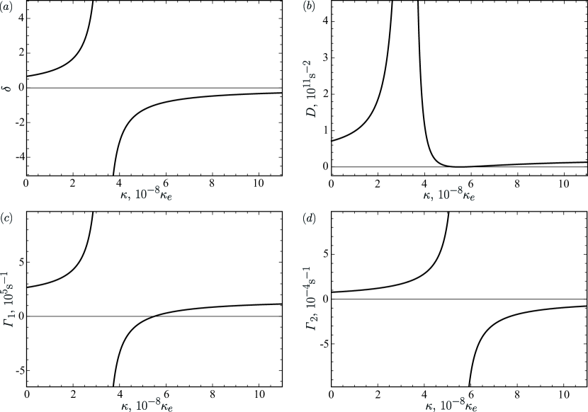
Figure 2.: Profiles depending on the thermal conductivity of the plasma: (a) parameter $\delta$ (Equation 10), (b) discriminant $D$, (c) root ${\it\Gamma}_{1}$, and (d) root ${\it\Gamma}_{2}$ of Equation 12. Thermal conductivity is measured in units of the classical electronic thermal conductivity calculated for $T=10^{6}$ K (Spitzer and Härm, 1953).fig2

As one can see, $|\,\delta\,|<1$ for all $\kappa$, except an interval $2\times 10^{-8}\,\kappa_{\,\rm e}<\kappa<6\times 10^{-8}\,\kappa_{\,\rm e}$. The sign of the parameter $\delta$ changes when the plasma thermal conductivity decreases to $\kappa\lesssim 3\times 10^{-8}\,\kappa_{\,\rm e}$. For example, if thermal conductivity is suppressed by a perturbation of the magnetic field, then ionic thermal conduction becomes more efficient (Rosenbluth and Kaufman, 1958)

$$\kappa_{\,\rm i}\approx 2\times 10^{-17}\,\frac{n^{2}}{T^{1/2}B^{\prime 2}}\,.$$

So in Section sec3, the thermal conductivity inside the current layer is suppressed by a perturbation of the magnetic field directed along the external magnetic field (for more details on the field configuration see Section sec3). The magnitude of the required perturbation of the magnetic field can be found from the evaluation $\kappa_{\,\rm i}\approx 3\times 10^{-8}\,\kappa_{\,\rm e}$. The amplitude of the magnetic field perturbation $B^{\prime}~{}\gtrsim~{}0.01~{}{\rm\,G}$ is sufficient to change the sign of the parameter $\delta$. This will be important for further discussion.

The roots of Equation 12 are as follows:

$${\it\Gamma}_{0}=0\,,$$

$${\it\Gamma}_{1,2}=\frac{1}{2}\left\{\left(\,\frac{1+\delta}{\tau_{\nu}}\,+\,\frac{-\alpha\,\delta}{\tau_{\lambda}}\,\right)\pm\left[\left(\,\frac{1+\delta}{\tau_{\nu}}\,+\,\frac{-\alpha\,\delta}{\tau_{\lambda}}\,\right)^{2}-4\,\frac{1}{\tau_{\nu}}\,\frac{(\beta-\alpha)\,\delta}{\tau_{\lambda}}\right]^{1/2}\right\}$$

The root ${\it\Gamma}_{0}$ is not of interest here, since it corresponds to the transition to a new stationary state, which differs from the initial one by the magnitude of the perturbation. The relation $\tau_{\nu}/\tau_{\lambda}$ is much smaller than 1 for the described conditions of the solar corona. Therefore, the roots ${\it\Gamma}_{1,2}$ can be expanded in small parameter $\tau_{\nu}/\tau_{\lambda}$. Keeping only zero-order terms, one obtains:

$${\it\Gamma}_{1}\simeq\frac{1+\delta}{\tau_{\nu}}\,,\qquad{\it\Gamma}_{2}\simeq\frac{\beta-\alpha}{\tau_{\lambda}}\,\frac{\delta}{1+\delta}\,.\ilabel{13}$$ (13)

Figure fig2b shows the dependence of the discriminant $D$ in Equation 12 on the thermal conductivity, while Figure fig2 c and d shows the roots ${\it\Gamma}_{1,2}$. The exact calculation of the roots ${\it\Gamma}_{1,2}$ completely coincides with the approximate Equations 13 in the scale of Figure fig2 c and d. Differences are observed only in the region of rapid growth of $|\,\delta\,|$, where the discriminant $D$ also tends to infinity, and in the region where the discriminant $D$ is negative (Figure fig2b). The root ${\it\Gamma}_{1}$ has a discontinuity in the first region (Figure fig2c), while the root ${\it\Gamma}_{2}$ has a discontinuity in the second region (Figure fig2d). In these areas, the linear approximation of the problem of small perturbations is unsuitable. Changing the initial parameters $n$, $T$, and $\sigma$ within the limits which are acceptable for the conditions of the solar corona stretches or compresses Figure fig2 along the coordinate axes, but does not make any qualitative changes in these plots.

The figure shows that ${\it\Gamma}_{1}\gg{\it\Gamma}_{2}$ for almost all values $\kappa$ except for a narrow interval near $\kappa=4\times 10^{-8}\,\kappa_{\,\rm e}$ where ${\it\Gamma}_{1}$ is negative and ${\it\Gamma}_{2}$ is positive. This means that the instability described by the root ${\it\Gamma}_{1}$ should grow much faster than the instability described by the root ${\it\Gamma}_{2}$ everywhere except in this narrow interval. In the geometry of the preflare current layer in the solar corona, the spatial scale of the root ${\it\Gamma}_{1}$ does not satisfy the MHD approximation used (Section sec4.1) and we should use a higher frequency approximation to study it further. Therefore, in what follows, we will focus on the root ${\it\Gamma}_{2}$ and assume that the value of the thermal conductivity satisfies the condition ${\it\Gamma}_{2}>{\it\Gamma}_{1}$.

3 Current Layer Model

sec3

We consider the piecewise homogeneous model of the preflare current layer, presented by Somov and Syrovatskii (1982). The current layer is located in the $(x,z)$ plane (Figure fig3). The $z$-axis complements the right triplet $(x,y,z)$ and is directed toward the reader in Figure fig3. The plasma concentration and temperature inside the layer are equal to $n_{s}$ and $T_{s}$, respectively. The current layer is assumed magnetically neutral, $B_{s}=0$, without any directed plasma flows, i.e. $v_{s}=0$. The half-thickness of the current layer $a$ is much smaller than its half-width $b$. When considering the preflare non-reconnecting current layer, $b\to\infty$ is assumed. As a consequence, $\partial/\partial{x}=0$ in such model. This means that we neglect the evolution of the current layer along the $x$-axis, such as the tearing instability (Furth, Killeen, and Rosenbluth, 1963). We focus on the structure of the current layer along the $z$-axis. The inner region of the current layer is separated from the outer plasma by a tangential discontinuity (Ledentsov and Somov, 2015b). Outside the layer, we denote the concentration and the temperature of the homogeneous plasma as $n_{0}$ and $T_{0}$, correspondingly. A uniform magnetic field $B_{0}$ is directed against the $x$-axis for positive $y$ and along the $x$-axis for negative $y$. Thus, the current in the layer is directed along the $z$-axis. In order to study the effect of thermal balance on the structural stability of a preflare current layer, the effects of viscosity, electrical and thermal conductivity, and radiative cooling are considered inside the current layer, but these effects are insignificant outside. An important difference between the model considered here and the Somov and Syrovatskii (1982) model is the possibility of penetration of a magnetic field perturbation inside the current layer. Mathematically, this comes to considering the current layer interior in the magnetohydrodynamic approximation rather than in the hydrodynamic one.

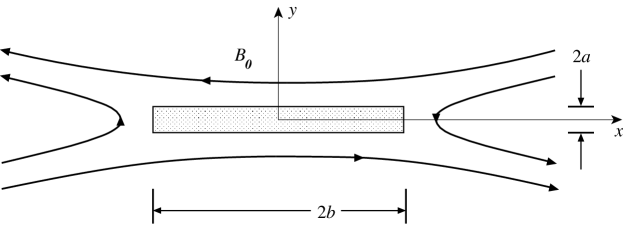
Figure 3.: Location of the current layer in the coordinate system.fig3

3.1 Outside the Current Layer

sec3.1

Following Somov and Syrovatskii (1982), we set $\sigma\to\infty$, $\kappa=0$, $\lambda=0$, $\eta=0$, and $\nu=0$ in the set of Equations 01 outside the current layer. Plasma density contrast inside and outside the super-hot turbulent-current layers is about 5 (see Section 8.5.3 in Somov, 2013). Kinetic models give the same values (Kolotkov, Vasko, and Nakariakov, 2015; Pascoe et al., 2017). Wherein, the external plasma could radiate up to a factor of 100 less efficiently than the internal one. In other words, the characteristic timescales of radiative processes outside the layer and those inside it (including the characteristic timescales of the perturbation and of the other non-adiabatic processes) could differ by two orders of magnitude, allowing one to neglect the effects of radiation in the external plasma. Moreover, we suppose that the considered preflare current layer is more similar to the neutral current layer by Syrovatskii, in which the density contrast can be much higher (Syrovatskii, 1976). In addition, the plasma is assumed to be at rest, i.e. $v_{0}=0$. The solution is sought in the form of a periodic perturbation along the $z$-axis in Figure fig3 which decays exponentially with distance from the current layer:

$$f(y,z,t)=f_{0}+f_{1}(y)\,{\rm exp}\,(-i\omega t+ik_{z}z)\,,$$

$$f_{1}(y)_{\rm top}=f_{\rm 1\,top}\,{\rm exp}\,[-k_{y1}(y-a)]\,,\qquad f_{1}(y)_{\rm bottom}=f_{\rm 1\,bottom}\,{\rm exp}\,[k_{y1}(y+a)]\,,$$

with perturbation amplitudes

$$f_{\rm 1\,top}\equiv\{{v_{y1},v_{z1},n_{1},T_{1},B_{x1}}\}\,,\qquad f_{\rm 1\,bottom}\equiv\{{-v_{y1},v_{z1},n_{1},T_{1},-B_{x1}}\}\,,$$

on either side outside the current layer, respectively. Here, $\omega$ is the perturbation frequency, $k_{z}$ and $k_{y1}$ are the perturbation wave numbers along the $z$ and $y$ axes, respectively, and $a$ is the half-thickness of the current layer. Index “$1$” refers to quantities outside the layer. Thus, we are looking for a solution in the form of a perturbation that propagates through the surface of the current layer and decays with distance from it.

Based on the symmetry of the problem, the set of Equations 01 is considered only for the upper half space. Neglecting the squares of the perturbed quantities, one finds the linearized system of equations:

$$i\omega\,n_{1}=-k_{y1}\,n_{0}v_{y1}+ik_{z}\,n_{0}v_{z1}\,,\ilabel{14}$$ (14)

$$i\omega\,\mu n_{0}v_{y1}=-k_{y1}\,2k_{{}_{\rm B}}(n_{0}T_{1}+T_{0}n_{1})+k_{y1}\,\frac{B_{0}}{4\pi}\,B_{x1}\,,\ilabel{15}$$ (15)

$$i\omega\,\mu n_{0}v_{z1}=ik_{z}\,2k_{{}_{\rm B}}(n_{0}T_{1}+T_{0}n_{1})-ik_{z}\,\frac{B_{0}}{4\pi}\,B_{x1}\,,\ilabel{16}$$ (16)

$$(\gamma-1)\,T_{0}n_{1}=n_{0}T_{1}\,,\ilabel{17}$$ (17)

$$i\omega\,B_{x1}=k_{y1}\,B_{0}v_{y1}-ik_{z}\,B_{0}\,v_{z1}\,.\ilabel{18}$$ (18)

The dispersion relation for perturbations outside the current layer is determined by equating the determinants of a homogeneous system of linear Equations 14 – 18 to zero

$$k_{y1}^{2}=k_{z}^{2}-\frac{\omega^{2}}{V_{S}^{2}+V_{A}^{2}}\,,\ilabel{19}$$ (19)

where the sound and the Alfvén speeds are denoted as

$$V_{S}=\sqrt{\frac{2\gamma k_{{}_{\rm B}}T_{0}}{\mu}}\,,\qquad V_{A}=\frac{B_{0}}{\sqrt{4\pi n_{0}\mu}}\,,\ilabel{20}$$ (20)

respectively. The dispersion relation in Equation 19 describes a fast magnetoacoustic wave propagating over the surface of the current layer perpendicular to the magnetic field.

3.2 Inside the Current Layer

sec3.2

Dissipative effects of Joule and viscous heating, thermal conductivity, and radiative cooling should be considered inside the current layer. The current layer is assumed magnetically neutral, $B_{s}=0$, without any directed plasma flows, i.e. $v_{s}=0$. The solution is sought in the same form as outside the current layer

$$f(y,z,t)=f_{s}+f_{2}(y)\,{\rm exp}\,(-i\omega t+ik_{z}z)\,.$$

The perturbations decrease exponentially along the $y$-axis when moving from the upper boundary of the current layer

$$f_{2}(y)_{\rm top}=f_{\rm 2\,top}\,{\rm exp}\,[-k_{y2}(a-y)]\,,$$

$$f_{\rm 2\,top}\equiv\frac{1}{2}\,{\rm exp}(k_{y2}a)\,\{v_{y2},v_{z2},n_{2},T_{2},B_{x2}\}\,$$

and when moving from the lower boundary

$$f_{2}(y)_{\rm bottom}=f_{\rm 2\,bottom}\,{\rm exp}\,[-k_{y2}(a+y)]\,,$$

$$f_{\rm 2\,bottom}\equiv\frac{1}{2}\,{\rm exp}(k_{y2}a)\,\{-v_{y2},v_{z2},n_{2},T_{2},-B_{x2}\}\,.$$

Here, index “$2$” refers to perturbations inside the layer, $\frac{1}{2}\,{\rm exp}(k_{y2}a)$ is a scale factor that unifies the solution for all thicknesses of the current layer. Inside the current layer, perturbations coming from the upper and lower boundaries add up

$$f_{2}(y)=f_{2}(y)_{\rm top}+f_{2}(y)_{\rm bottom}\,.$$

The resulting dependences of the perturbations on the coordinate $y$ are hyperbolic functions. The sum of the perturbations which are odd in the $y$ direction gives a hyperbolic sine

$$\left\{\begin{array}[]{c}v_{y2}(y)\\ B_{x2}(y)\end{array}\right\}=\left\{\begin{array}[]{c}v_{y2}\\ B_{x2}\end{array}\right\}{\rm sinh}\,(k_{y2}y)\,,$$

The sum of the perturbations which are even in $y$ gives a hyperbolic cosine

$$\left\{\begin{array}[]{c}v_{z2}(y)\\ n_{2}(y)\\ T_{2}(y)\end{array}\right\}=\left\{\begin{array}[]{c}v_{z2}\\ n_{2}\\ T_{2}\end{array}\right\}{\rm cosh}\,(k_{y2}y)\,.$$

Real values of $k_{y2}$ determine the effective thickness of the skin depth of the layer, that is, the distance to which the disturbance of the layer boundary penetrates. On the other hand, a standing wave is formed inside the current layer along the $y$-axis at imaginary $k_{y2}$. The value of the wave number $k_{y2}$ is not prescribed and can be determined from the solution, however, this is not the purpose of this article. The solution describes the plasma motion which is symmetric about the $(x,z)$ plane.

The set of Equations 01 is linearized as in the previous section:

$$i\omega\,n_{2}=k_{y2}\,n_{s}v_{y2}+ik_{z}\,n_{s}v_{z2}\,,\ilabel{21}$$ (21)

$$i\omega\,\mu n_{s}v_{y2}=k_{y2}\,2k_{{}_{\rm B}}(n_{s}T_{2}+T_{s}n_{2})+(k_{z}^{2}-k_{y2}^{2})\,\eta v_{y2}-i\omega k_{y2}\frac{\nu}{n_{s}}n_{2}\,,\ilabel{22}$$ (22)

$$i\omega\,\mu n_{s}v_{z2}=ik_{z}\,2k_{{}_{\rm B}}(n_{s}T_{2}+T_{s}n_{2})+(k_{z}^{2}-k_{y2}^{2})\,\eta v_{z2}-i\omega ik_{z}\frac{\nu}{n_{s}}n_{2}\,,\ilabel{23}$$ (23)

$$i\omega\,\frac{2k_{{}_{\rm B}}n_{s}}{\gamma-1}\,T_{2}-i\omega\,2k_{{}_{\rm B}}T_{s}\,n_{2}=(k_{z}^{2}-k_{y2}^{2})\,\kappa T_{2}+\frac{\partial\lambda}{\partial T}\,T_{2}+\frac{\partial\lambda}{\partial n}\,n_{2}\,,\ilabel{24}$$ (24)

$$i\omega\,B_{x2}=(k_{z}^{2}-k_{y2}^{2})\,\nu_{m}B_{x2}\,.\ilabel{25}$$ (25)

Equation 25, like the set of Equations 05 and 06, can be satisfied at $B_{x2}=0$, however, if the perturbation of the magnetic field, $B_{x2}\neq 0$, penetrates into the current layer, then Equation 25 gives an additional dispersion relation independent of the $B_{x2}$ value. After expressing the difference $k_{z}^{2}-k_{y2}^{2}$ from Equation 25, we can exclude it from the remaining Equation 21 – 25. Making transformations similar to those in Section sec2.1, gives again Equation 12 with $n=n_{s}$ and $T=T_{s}$. It is worth noting that the possibility to directly determine the instability increment is due to the simultaneous presence of two dispersion relations in Equations 21 – 25 at once: the first follows from Equations 21 – 24, and the second one from Equation 25. An important feature of Equations 21 – 25 is that the wave vector $k_{z}$ turns out to be perpendicular to the arising perturbation of the magnetic field $B_{x2}$. This promotes the suppression of thermal conductivity along the $z$-axis (in the direction of the current) and the formation of a thermal instability (see Section sec2.2).

3.3 Boundary of the Current Layer

sec3.3

The considered model of the current layer has no plasma motion neither outside nor inside the layer in equilibrium ($v_{0}=0,v_{s}=0$), but a magnetic field jump occurs at the layer boundary. A tangential discontinuity in MHD corresponds to such conditions (Ledentsov and Somov, 2015a).

The sum of the gas-dynamic and magnetic pressure should be equal on the different sides of the tangential discontinuity (Syrovatskii, 1956). In a linearized form, it looks as follows

$$n_{0}T_{1}+T_{0}n_{1}-\frac{B_{0}B_{x1}}{8\pi k_{{}_{\rm B}}}=(n_{s}T_{2}+T_{s}n_{2})\,{\rm cosh}\,(k_{y2}a)\,.\ilabel{26}$$ (26)

The left side of Equation 26 can be expressed in terms of the perturbation $v_{y1}$ using Equation 15. The right side of Equation 26 can be expressed in terms of the perturbation $v_{y2}$ using Equations 21 – 23 and substituting $k_{z}^{2}-k_{y2}^{2}$ from Equation 25. Then Equation 26 takes the form

$$-\,\frac{n_{0}}{n_{s}}\,\frac{v_{y1}}{k_{y1}}=\frac{\tau_{\nu}}{\tau_{\sigma}}\,\frac{v_{y2}}{k_{y2}}\,{\rm cosh}\,(k_{y2}a)\,.\ilabel{27}$$ (27)

Here, the Equations 09 are also used with substitutions $n=n_{s}$ and $T=T_{s}$.

Velocity perturbations distort the surface of the tangential discontinuity. For reasons of continuity, the velocity perturbation on both sides of the discontinuity should have the same magnitude and direction

$$v_{y1}^{2}+v_{z1}^{2}=v_{y2}^{2}\,{\rm sinh}^{2}\,(k_{y2}a)+v_{z2}^{2}\,{\rm cosh}^{2}\,(k_{y2}a)\,,\ilabel{28}$$ (28)

$$\frac{v_{z1}}{v_{y1}}=\frac{v_{z2}\,{\rm cosh}\,(k_{y2}a)}{v_{y2}\,{\rm sinh}\,(k_{y2}a)}\,.\ilabel{29}$$ (29)

Equation 28 is then rewritten as

$$v_{y1}=\pm\,v_{y2}\,{\rm sinh}\,(k_{y2}a)\,,\ilabel{30}$$ (30)

where the choice of sign depends on the signs of perturbations $v_{y1}$ and $v_{z1}$.

Let us divide Equation 30 by Equation 27

$$\pm\,\frac{\tau_{\nu}}{\tau_{\sigma}}\,\frac{n_{s}}{n_{0}}\,k_{y1}=k_{y2}\,{\rm tanh}\,(k_{y2}a)\,.\ilabel{31}$$ (31)

Equation 31 differs from Equation 23 of Somov and Syrovatskii (1982) by a coefficient $\tau_{\nu}/\tau_{\sigma}$ determining the role of viscosity in the formation of the structure of the preflare current layer. Note that the right side of Equation 31 is positive for any real $k_{y2}$. This means that $\pm(\tau_{\nu}/\tau_{\sigma})$ should also be positive for physically meaningful values $k_{y1}$. Substitution of the wave numbers $k_{y1}$ and $k_{y2}$ from Equations 19 and 25, respectively, gives the dispersion relation which relates the instability increment to the wave number $k_{z}$

$$\left(\frac{\tau_{\nu}}{\tau_{\sigma}}\,\frac{n_{s}}{n_{0}}\right)^{2}\left[k_{z}^{2}+\frac{{\it\Gamma}^{2}}{V_{S}^{2}+V_{A}^{2}}\right]=\left[\,k_{z}^{2}+\frac{{\it\Gamma}}{\nu_{m}}\,\right]{\rm tanh}^{2}\left\{a\left[\,k_{z}^{2}+\frac{{\it\Gamma}}{\nu_{m}}\,\right]^{1/2}\right\}\,.\ilabel{32}$$ (32)

We determine the growth increment, ${\it\Gamma}=-i\omega$, from Equation 12, which is identical to the solution of Equations 21 – 25. Then we determine the spatial period of the instability, $l=2\pi/k_{z}$, from Equation 32.

4 Thermal Instability of the Current Layer

sec4

Now the growth rate of the instability can be calculated using Equation 12 and the corresponding spatial period of the perturbation can be found from Equation 32. For this aim, the appropriate values of the parameters of the current layer and the surrounding plasma should be chosen. Taking into account the possibility of plasma gathering by magnetic fields and its heating during the formation of the current layer before the onset of the studied instability, the range of values $n_{0}=10^{8}-10^{12}{\rm\,cm}^{-3}$, $n_{s}/n_{0}=10-10^{3}$, $T_{0}=10^{6}{\rm\,K}$, $T_{s}=10^{6}-10^{8}{\rm\,K}$, $B_{0}=1-10^{2}{\rm\,G}$, $\sigma=10^{11}{\rm\,s}^{-1}$, $a=10^{5}-10^{7}{\rm\,cm}$ is considered. This range covers all the reasonable parameters of the coronal plasma. As one can see from the first two brackets on the left hand side of Equation 32, the effect of an increase of viscosity is the opposite to an increase in the density jump. Therefore, no viscosity is introduced, because its effect is taken into account in the density jump ($\eta=0$, $\nu=0$). In addition, the viscosity effect is small ($\tau_{\nu}\approx\tau_{\sigma}$) in the investigated range of coronal plasma parameters.

4.1 Growth Increment in the Current Layer

sec4.1

The instability occurs when the roots of Equation 12 are positive. The roots ${\it\Gamma}_{1}$ and ${\it\Gamma}_{2}$ are real numbers everywhere except for a narrow interval where $D<0$ (Figure fig2b). In this interval, the roots become complex. Three unstable solutions are possible: the left branch of ${\it\Gamma}_{1}$ (Figure fig2c), the positive part of the right branch of ${\it\Gamma}_{1}$ (also Figure fig2c), and the left branch of ${\it\Gamma}_{2}$ (Figure fig2d). As one can see, $|\,{\it\Gamma}_{1}\,|\gg|\,{\it\Gamma}_{2}\,|$ everywhere except perhaps in a small area near $D=0$ (see Figure fig2b). Calculation of the instability scale over the entire range of coronal plasma parameters described above gives $l\lesssim 10^{4}{\rm\,cm}$. It is less than the corresponding Larmor radius of the proton for most of the values of plasma parameters. Moreover, complex values of ${\it\Gamma}_{1}$ for $D<0$ lead to complex values of $k_{z}$, which corresponds to the spatial attenuation of the perturbation at the same scales ($l\lesssim 10^{4}{\rm\,cm}$). The presence of viscosity can only increase the value ${\it\Gamma}_{1}$ as seen from Equations 11 and 13. Therefore, it further reduces the scale of instability.

The MHD approximation is incorrect for the description of the plasma at such scales. Therefore, in this article we cannot say whether such instability appears in a more general kinetic description. Remaining within the framework of the MHD, we further consider the root ${\it\Gamma}_{1}$ physically meaningless. In any case, if the instability associated with the root ${\it\Gamma}_{1}$ exists in the kinetic description and dominates the instability with an increment ${\it\Gamma}_{2}$, there is a narrow interval of plasma thermal conductivities $\kappa$ where ${\it\Gamma}_{1}$ is negative and ${\it\Gamma}_{2}$ is positive, and an instability occurs due to the root ${\it\Gamma}_{2}$ (Figure fig2). We assume that the thermal conductivity is suppressed by the perturbation of the magnetic field in the current layer, which triggers the instability. Note that, for further reasoning, it is not important which process led to the suppression of the thermal conductivity. The space scale of the instability 32 does not depend on the exact value of the thermal conductivity coefficient and can be calculated for any range of coronal plasma parameters.

The negative right branch of the root ${\it\Gamma}_{2}$ indicates the stabilizing effect of the high thermal conductivity of the plasma. However, if, for some reason, the thermal conductivity falls below the threshold value $\delta=-1$ (see Equation 13 and Figure fig2d), ${\it\Gamma}_{2}$ becomes positive and an instability occurs. The value $\beta-\alpha$ is positive over the entire range of the above-described coronal plasma conditions. As it was shown in Section sec2.2, the transverse magnetic field can cause a decrease of the thermal conductivity. Equations 21 – 25 allow the perturbations of the $x$-component of the magnetic field to appear inside the current layer. This field is actually perpendicular to $\nabla T$ in the current layer under consideration. However, the specific nature of the suppression of the thermal conductivity is not very important for further considerations. It is enough for us to assume that the thermal conductivity went down for some reason ($\tau_{\kappa}\ll\tau_{\sigma}$). Then the growth rate of the instability tends to the value

$${\it\Gamma}=\frac{2}{5}\,\frac{\beta-\alpha}{\tau_{\lambda}}\ilabel{33}$$ (33)

(see Equations 13 and 10). The growth time of the instability is proportional to the characteristic time of the plasma cooling and depends on the logarithmic derivatives of the radiative cooling function (with respect to concentration and temperature). Thermal instability criteria (Field, 1965) in our notation can be written as follows:

$$\alpha<0\qquad$$

$$\alpha<\beta-1\qquad$$

$$\alpha<-\frac{\beta-1}{\gamma-1}\qquad$$

where $\beta=2$, $\gamma=5/3$. Thus, the criteria for isochoric, isobaric, and isentropic instabilities are $\alpha<0$, $\alpha<1$, and $\alpha<-3/2$, respectively. Figure fig1b shows that the isobaric criterion of thermal instability is fulfilled for the entire range of coronal plasma parameters. We expect that the instability discussed in this work is a special case of the condensation mode of the isobaric thermal instability.

4.2 Spatial Period in the Current Layer

sec4.2

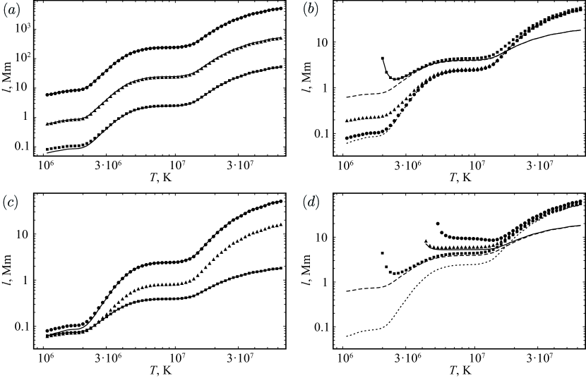
Figure 4.: The spatial period of the instability depending on the temperature of the current layer. Parameters of the coronal plasma: $n_{0}=10^{10}{\rm\,cm}^{-3}$, $n_{s}/n_{0}=10$, $a=10^{5}{\rm\,cm}$, $B_{0}=100{\rm\,G}$. One of the parameters changes in each figure: (a) $n_{0}=10^{8}{\rm\,cm}^{-3}$ (circles), $n_{0}=10^{9}{\rm\,cm}^{-3}$ (triangles), $n_{0}=10^{10}{\rm\,cm}^{-3}$ (squares), solid lines show analytical solutions (Equation 35); (b) $n_{s}/n_{0}=10$ (circles), $n_{s}/n_{0}=100$ (triangles), $n_{s}/n_{0}=1000$ (squares), dotted line shows the analytical solution (Equation 35) for circles, solid and dashed lines show analytical solutions for Equation 36 and 37, respectively, for squares; (c) $a=10^{5}{\rm\,cm}$ (circles), $a=3\times 10^{5}{\rm\,cm}$ (triangles), $a=10^{7}{\rm\,cm}$ (squares), upper and lower solid lines show analytical solutions for Equation 35 and 37, respectively; (d) $n_{s}/n_{0}=1000$, $B_{0}=1{\rm\,G}$ (circles), $B_{0}=10{\rm\,G}$ (triangles), $B_{0}=100{\rm\,G}$ (squares) dotted line shows analytical solution (Equation 35) for circles, solid line shows analytical solution (Equation 36) for triangles, dashed line shows analytical solution (Equation 37) for squares. fig4

Equation 32 has two obvious approximations: ${\rm tanh}\,(k_{y2}a)\to k_{y2}a$ for small $k_{y2}a$ and ${\rm tanh}\,(k_{y2}a)\to 1$ for large $k_{y2}a$. In what follows, they are called the thin and thick approximations, respectively. In the first case, the current layer is thin enough, so that the perturbation arising at one boundary of the layer does not decay along the way to the other boundary. On the contrary, the current layer is quite thick compared to the attenuation length of the perturbation in the second case. Numerical calculations of Equation 32 with ${\it\Gamma}$ from Equation 33 show that $k_{z}^{2}\ll{\it\Gamma}/\nu_{m}$ over the entire range of coronal plasma parameters. Therefore, the dispersion Equation 32 can be simplified.

In the thin approximation,

$$k_{z{\rm thin}}^{2}\simeq\left[\left(\frac{\tau_{\sigma}}{\tau_{\nu}}\,\frac{n_{0}}{n_{s}}\right)^{2}\frac{1}{V_{D}^{2}}-\frac{1}{V_{S}^{2}+V_{A}^{2}}\right]\,{\it\Gamma}^{2}\,,\ilabel{34}$$ (34)

where the drift velocity $V_{D}=\nu_{m}/a$ is introduced. This is the velocity at which the plasma drifts into the current layer (see Section 8.1.1 in Somov, 2013). There is no drift in our model, but we will use this notation for convenience. For sufficiently strong magnetic field (see Equation 20) and low viscosity, Equation 34 transforms to

$$k_{z{\rm thin}}\simeq\frac{n_{0}}{n_{s}}\,\frac{{\it\Gamma}}{V_{D}}\,.\ilabel{35}$$ (35)

In the thick approximation,

$$k_{z{\rm thick}}^{2}\simeq\left(\frac{\tau_{\sigma}}{\tau_{\nu}}\,\frac{n_{0}}{n_{s}}\right)^{2}\frac{{\it\Gamma}}{\nu_{m}}-\frac{{\it\Gamma}^{2}}{V_{S}^{2}+V_{A}^{2}}\,,\ilabel{36}$$ (36)

and for strong field and low viscosity,

$$k_{z{\rm thick}}\simeq\frac{n_{0}}{n_{s}}\,\sqrt{\frac{{\it\Gamma}}{\nu_{m}}}\,.\ilabel{37}$$ (37)

Figure fig4 shows a series of profiles of the dependence for the spatial period of the instability calculated as $l=2\pi/k_{z}$ for $k_{z}$ from Equation 32 (circles, triangles, and squares) and $k_{z{\rm thin}}$ and $k_{z{\rm thick}}$ approximations from Equations 35 and 37, respectively (thin lines), on the temperature of the current layer. The exact calculation of Equations 12 and 32 is shown by circles, triangles, and squares in the figure. The approximative Equations 35 – 37 are shown by solid, dashed, and dotted lines.

The spatial period of the instability strongly depends on the concentration of the surrounding plasma (Figure fig4a). The graphs are in good agreement with the thin approximation (Equation 35). Using Equation 34 instead of Equation 35 does not lead to a visible improvement in the result. The most remarkable feature of the graphs is a step at $T_{s}=5\times 10^{6}-10^{7}{\rm\,K}$. The spatial period is constant in a fairly wide temperature range, and it is this temperature range that seems quite reasonable for a preflare current layer. It is also reasonable to expect an increase in plasma concentration near the current layer. With an increase in the strength of the magnetic field from 1 G (for a quiet corona) to 100 G (for the active region), the plasma concentration also increases by two orders of magnitude due to magnetic freezing. Therefore, $n_{0}=10^{10}{\rm\,cm}^{-3}$ is used for the other graphs in Figure fig4.

An increase in the concentration jump does not change the spatial period quantitatively, but it changes the solution qualitatively (Figure fig4b). Large density jumps at low temperatures $T_{s}<10^{7}$ correspond to a thick approximation, and Equation 36 follows the exact solution much better than Equation 37.

An increase in the half-thickness of the current layer obviously leads to a thick approximation, but it also slightly changes the spatial period of instability (Figure fig4c).

The influence of the magnetic field is manifested only at high jumps in concentration when the second term on the right side of the Equations 34 and 36 prevails. Therefore, Figure fig4d is calculated for $n_{s}/n_{0}=1000$. Again, the dependence of the spatial period on the magnitude of the magnetic field is rather weak. The influence of the magnetic field becomes indistinguishable at lower density contrasts.

As a result, the spatial period of the instability is constant over a wide range of changes in the parameters of the coronal plasma at the assumed temperature of the preflare current layer $T_{s}=5\times 10^{6}-10^{7}{\rm\,K}$ and the concentration of the surrounding plasma $n_{0}=10^{10}{\rm\,cm}^{-3}$. Its values belong to in a narrow range from 1 to 10 Mm, which is in good agreement with the distances between the solar flare loops observed in the ultraviolet range.

5 Conclusion

sec5

The stability problem of the preflare current layer with respect to small perturbations is addressed. The problem is solved within the framework of dissipative MHD taking into account viscosity, electrical and thermal conductivity, and radiative cooling of the plasma. A piecewise homogeneous current layer model is used. The simplicity of the model allows one to obtain accurate analytical expressions for the growth rate (Equation 12) and the spatial scale (Equation 32) of instability, as well as their simple approximations (Equations 33 – 37) in the conditions of the solar corona. The instability has a thermal nature. It occurs as a result of a drop in thermal conductivity inside the current layer and increases on the characteristic time scale of radiative plasma cooling. Due to the structural features of the radiative loss function of an optically thin medium, the spatial instability period is contained in a narrow range of values of about $l=1-10{\rm\,Mm}$ for a wide range of parameters of the current layer and the surrounding plasma.

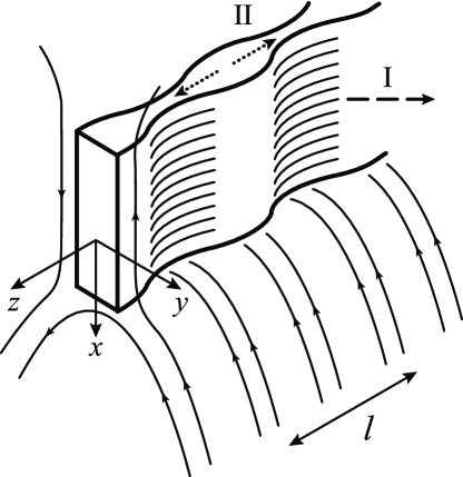
Figure 5.: Location of the perturbed current layer above the arcade of coronal magnetic loops. The perturbation has a spatial period $l$. The Roman numbers mark the energy fluxes associated with radiative plasma cooling (I) and heat conduction (II).fig5

The instability properties allow us to offer the following qualitative picture of the solar flare triggering. There is a preflare current layer above the arcade of coronal magnetic loops (Figure fig5). Due to a random perturbation, some of its sections begin to lose more heat by radiation. High electronic thermal conductivity can redistribute heat between cold and hot areas. However, if the electronic thermal conductivity is suppressed by the perturbation of the transverse magnetic field penetrating in the current layer, then the ionic thermal conductivity does not have time to transfer heat from hot to cold areas. The temperature difference between the cold and hot sections of the preflare current layer increases with increment described by Equation 33. The alternation of cold and hot sections leads to a wave-like curvature of the surface of the current layer with a spatial period $l$ due to the total pressure balance. The curvature has a symmetrical shape in accordance with the solution found. The current layer begins to disintegrate into individual fibers located across the direction of the current, which can lead to its breaking and, as a result, to a solar flare. The regions of the main energy release will alternate with the same spatial period $l$. Flows of accelerated charged particles rush into the coronal magnetic loops located near the regions of energy release, which ultimately leads to the observed brightening of individual flare loops in the ultraviolet range.

In order to mathematically simplify the model, many significant physical features of the preflare current layer were neglected. Magnetic non-neutrality of the current layer leads to a change in the pressure balance at its boundary, while the appearance of a component of the magnetic field normal to the layer changes the type of MHD discontinuity on the boundary (Somov and Titov, 1985a, b). The finite width of the current layer requires taking into account the corresponding derivatives with respect to the $x$ coordinate, which leads to the appearance of tearing instability (Somov and Verneta, 1988, 1989). The observations of flare loops on the Sun indirectly indicate a complex current layer geometry that is different from a simple planar configuration. A statistical analysis of the flare loops themselves in the context of the considered model is a separate complex task. Attention on these and other issues will be paid in following articles of this series (Thermal Trigger for Solar Flares).

Acknowledgments

The author thanks Prof. Boris Somov, Vasilisa Nikiforova, and anonymous reviewer for discussing the article.

Disclosure of Potential Conflicts of Interest The author declares that there are no conflicts of interest.

References

- Antolin (2020) Antolin, P.: 2020, Thermal instability and non-equilibrium in solar coronal loops: from coronal rain to long-period intensity pulsations. Plasma Phys. Contr. F. 62, 014016. DOI. ADS.
- Artemyev and Zimovets (2012) Artemyev, A., Zimovets, I.: 2012, Stability of Current Sheets in the Solar Corona. Sol. Phys. 277, 283. DOI. ADS.
- Aulanier et al. (2000) Aulanier, G., DeLuca, E.E., Antiochos, S.K., McMullen, R.A., Golub, L.: 2000, The Topology and Evolution of the Bastille Day Flare. ApJ 540, 1126. DOI. ADS.
- Benz (2017) Benz, A.O.: 2017, Flare Observations. Living Rev. Sol. Phys. 14, 2. DOI. ADS.
- Carbonell et al. (2006) Carbonell, M., Terradas, J., Oliver, R., Ballester, J.L.: 2006, Spatial damping of linear non-adiabatic magnetoacoustic waves in a prominence medium. A&A 460, 573. DOI. ADS.
- Claes and Keppens (2019) Claes, N., Keppens, R.: 2019, Thermal stability of magnetohydrodynamic modes in homogeneous plasmas. A&A 624, A96. DOI. ADS.
- De Moortel and Hood (2004) De Moortel, I., Hood, A.W.: 2004, The damping of slow MHD waves in solar coronal magnetic fields. II. The effect of gravitational stratification and field line divergence. A&A 415, 705. DOI. ADS.
- Dere et al. (2019) Dere, K.P., Del Zanna, G., Young, P.R., Landi, E., Sutherland, R.S.: 2019, CHIANTI—An Atomic Database for Emission Lines. XV. Version 9, Improvements for the X-Ray Satellite Lines. ApJS 241, 22. DOI. ADS.
- Field (1965) Field, G.B.: 1965, Thermal Instability. ApJ 142, 531. DOI. ADS.
- Furth, Killeen, and Rosenbluth (1963) Furth, H.P., Killeen, J., Rosenbluth, M.N.: 1963, Finite-Resistivity Instabilities of a Sheet Pinch. Phys. Fluids 6, 459. DOI. ADS.
- Hollweg (1986) Hollweg, J.V.: 1986, Viscosity and the Chew-Goldberger-Low Equations in the Solar Corona. ApJ 306, 730. DOI. ADS.
- Hood (1992) Hood, A.W.: 1992, Instabilities in the solar corona. Plasma Phys. Contr. F. 34, 411. DOI. ADS.
- Ibanez S. and Escalona T. (1993) Ibanez S., M.H., Escalona T., O.B.: 1993, Propagation of Hydrodynamic Waves in Optically Thin Plasmas. ApJ 415, 335. DOI. ADS.
- Klimchuk (2019) Klimchuk, J.A.: 2019, The Distinction Between Thermal Nonequilibrium and Thermal Instability. Sol. Phys. 294, 173. DOI. ADS.
- Klimushkin et al. (2017) Klimushkin, D.Y., Nakariakov, V.M., Mager, P.N., Cheremnykh, O.K.: 2017, Corrugation Instability of a Coronal Arcade. Sol. Phys. 292, 184. DOI. ADS.
- Kolotkov, Duckenfield, and Nakariakov (2020) Kolotkov, D.Y., Duckenfield, T.J., Nakariakov, V.M.: 2020, Seismological constraints on the solar coronal heating function. A&A 644, A33. DOI. ADS.
- Kolotkov, Nakariakov, and Zavershinskii (2019) Kolotkov, D.Y., Nakariakov, V.M., Zavershinskii, D.I.: 2019, Damping of slow magnetoacoustic oscillations by the misbalance between heating and cooling processes in the solar corona. A&A 628, A133. DOI. ADS.
- Kolotkov, Vasko, and Nakariakov (2015) Kolotkov, D.Y., Vasko, I.Y., Nakariakov, V.M.: 2015, Kinetic model of force-free current sheets with non-uniform temperature. Phys. Plasmas 22, 112902. DOI. ADS.
- Krucker, Hurford, and Lin (2003) Krucker, S., Hurford, G.J., Lin, R.P.: 2003, Hard X-Ray Source Motions in the 2002 July 23 Gamma-Ray Flare. ApJ 595, L103. DOI. ADS.
- Ledentsov and Somov (2015a) Ledentsov, L.S., Somov, B.V.: 2015a, Discontinuous plasma flows in magnetohydrodynamics and in the physics of magnetic reconnection. Phys. Uspekhi 58, 107. DOI. ADS.
- Ledentsov and Somov (2015b) Ledentsov, L.S., Somov, B.V.: 2015b, MHD discontinuities in solar flares: Continuous transitions and plasma heating. Adv. Space Res. 56, 2779. DOI. ADS.
- Nakariakov and Kolotkov (2020) Nakariakov, V.M., Kolotkov, D.Y.: 2020, Magnetohydrodynamic Waves in the Solar Corona. ARA&A 58, 441. DOI. ADS.
- Nakariakov et al. (2006) Nakariakov, V.M., Foullon, C., Verwichte, E., Young, N.P.: 2006, Quasi-periodic modulation of solar and stellar flaring emission by magnetohydrodynamic oscillations in a nearby loop. A&A 452, 343. DOI. ADS.
- Nakariakov et al. (2017) Nakariakov, V.M., Afanasyev, A.N., Kumar, S., Moon, Y.-J.: 2017, Effect of Local Thermal Equilibrium Misbalance on Long-wavelength Slow Magnetoacoustic Waves. ApJ 849, 62. DOI. ADS.
- Oreshina and Somov (1998) Oreshina, A.V., Somov, B.V.: 1998, Slow and fast magnetic reconnection. I. Role of radiative cooling. A&A 331, 1078. ADS.
- Pascoe et al. (2017) Pascoe, D.J., Anfinogentov, S., Nisticò, G., Goddard, C.R., Nakariakov, V.M.: 2017, Coronal loop seismology using damping of standing kink oscillations by mode coupling. II. additional physical effects and Bayesian analysis. A&A 600, A78. DOI. ADS.
- Perelomova (2020) Perelomova, A.: 2020, On description of periodic magnetosonic perturbations in a quasi-isentropic plasma with mechanical and thermal losses and electrical resistivity. Phys. Plasmas 27, 032110. DOI. ADS.
- Priest and Forbes (2002) Priest, E.R., Forbes, T.G.: 2002, The magnetic nature of solar flares. A&A Rev. 10, 313. DOI. ADS.
- Reva et al. (2015) Reva, A., Shestov, S., Zimovets, I., Bogachev, S., Kuzin, S.: 2015, Wave-like Formation of Hot Loop Arcades. Sol. Phys. 290, 2909. DOI. ADS.
- Rosenbluth and Kaufman (1958) Rosenbluth, M.N., Kaufman, A.N.: 1958, Plasma Diffusion in a Magnetic Field. Phys. Rev. 109, 1. DOI. ADS.
- Rosner, Tucker, and Vaiana (1978) Rosner, R., Tucker, W.H., Vaiana, G.S.: 1978, Dynamics of the quiescent solar corona. ApJ 220, 643. DOI. ADS.
- Schmelz et al. (2012) Schmelz, J.T., Reames, D.V., von Steiger, R., Basu, S.: 2012, Composition of the Solar Corona, Solar Wind, and Solar Energetic Particles. ApJ 755, 33. DOI. ADS.
- Somov (2012) Somov, B.V.: 2012, Plasma Astrophysics. Part I: Fundamentals and Practice. Second Edition 391, Astrophys. Space Sci. Library, ASSL. DOI. ADS.
- Somov (2013) Somov, B.V.: 2013, Plasma Astrophysics. Part II: Reconnection and Flares. Second Edition 392, Astrophys. Space Sci. Library, ASSL. DOI. ADS.
- Somov and Oreshina (2000) Somov, B.V., Oreshina, A.V.: 2000, Slow and fast magnetic reconnection. II. High-temperature turbulent-current sheet. A&A 354, 703. ADS.
- Somov and Syrovatskii (1982) Somov, B.V., Syrovatskii, S.I.: 1982, Thermal Trigger for Solar Flares and Coronal Loops Formation. Sol. Phys. 75, 237. DOI. ADS.
- Somov and Titov (1985a) Somov, B.V., Titov, V.S.: 1985a, Magnetic Reconnection in a High Temperature Plasma of Solar Flares. Sol. Phys. 95, 141. DOI. ADS.
- Somov and Titov (1985b) Somov, B.V., Titov, V.S.: 1985b, Magnetic Reconnection in a High-Temperature Plasma of Solar Flares - Part Two - Effects Caused by Transverse and Longitudinal Magnetic Fields. Sol. Phys. 102, 79. DOI. ADS.
- Somov and Verneta (1988) Somov, B.V., Verneta, A.I.: 1988, Magnetic Reconnection in High-Temperature Plasma of Solar Flares - Part Three. Sol. Phys. 117, 89. DOI. ADS.
- Somov and Verneta (1989) Somov, B.V., Verneta, A.I.: 1989, Magnetic Reconnection in a High-Temperature Plasma of Solar Flares - Part Four. Sol. Phys. 120, 93. DOI. ADS.
- Somov and Verneta (1993) Somov, B.V., Verneta, A.I.: 1993, Tearing Instability of Reconnecting current Sheets in Space Plasmas. Space Sci. Rev. 65, 253. DOI. ADS.
- Somov, Dzhalilov, and Staude (2007) Somov, B.V., Dzhalilov, N.S., Staude, J.: 2007, Peculiarities of entropy and magnetosonic waves in optically thin cosmic plasma. Astron. Lett.+ 33, 309. DOI. ADS.
- Somov et al. (2002) Somov, B.V., Kosugi, T., Hudson, H.S., Sakao, T., Masuda, S.: 2002, Magnetic Reconnection Scenario of the Bastille Day 2000 Flare. ApJ 579, 863. DOI. ADS.
- Spitzer and Härm (1953) Spitzer, L., Härm, R.: 1953, Transport Phenomena in a Completely Ionized Gas. Phys. Rev. 89, 977. DOI. ADS.
- Syrovatskii (1956) Syrovatskii, S.I.: 1956, Some properties of discontinuity surfaces in magnetohydrodynamics. Tr. Fiz. Inst. im. P.N. Lebedeva, Akad. Nauk SSSR [in Russian] 8, 13.
- Syrovatskii (1958) Syrovatskii, S.I.: 1958, Magnetohydrodynamik. Fortschritte der Physik 6, 437. DOI. ADS.
- Syrovatskii (1976) Syrovatskii, S.I.: 1976, Current-sheet parameters and a thermal trigger for solar flares. Sov. Astron. Lett.+ 2, 13. ADS.
- Toriumi and Wang (2019) Toriumi, S., Wang, H.: 2019, Flare-productive active regions. Living Rev. Sol. Phys. 16, 3. DOI. ADS.
- Uzdensky (2007) Uzdensky, D.A.: 2007, The Fast Collisionless Reconnection Condition and the Self-Organization of Solar Coronal Heating. ApJ 671, 2139. DOI. ADS.
- Vorpahl (1976) Vorpahl, J.A.: 1976, The triggering and subsequent development of a solar flare. ApJ 205, 868. DOI. ADS.
- Weibel (1959) Weibel, E.S.: 1959, Spontaneously Growing Transverse Waves in a Plasma Due to an Anisotropic Velocity Distribution. Phys. Rev. Lett. 2, 83. DOI. ADS.
- Zavershinskii et al. (2019) Zavershinskii, D.I., Kolotkov, D.Y., Nakariakov, V.M., Molevich, N.E., Ryashchikov, D.S.: 2019, Formation of quasi-periodic slow magnetoacoustic wave trains by the heating/cooling misbalance. Phys. Plasmas 26, 082113. DOI. ADS.