Light Dirac neutrino portal dark matter with observable $\Delta{N_{\rm eff}}$

Abstract

We propose a Dirac neutrino portal dark matter scenario by minimally extending the particle content of the Standard Model (SM) with three right handed neutrinos ($\nu_{R}$), a Dirac fermion dark matter candidate ($\psi$) and a complex scalar ($\phi$), all of which are singlets under the SM gauge group. An additional $\mathbb{Z}_{4}$ symmetry has been introduced for the stability of dark matter candidate $\psi$ and also ensuring the Dirac nature of light neutrinos at the same time. Both the right handed neutrinos and the dark matter thermalise with the SM plasma due to a new Yukawa interaction involving $\nu_{R}$, $\psi$ and $\phi$ while the latter maintains thermal contact via the Higgs portal interaction. The decoupling of $\nu_{R}$ occurs when $\phi$ loses its kinetic equilibrium with the SM plasma and thereafter all three $\mathbb{Z}_{4}$ charged particles form an equilibrium among themselves with a temperature $T_{\nu_{R}}$. The dark matter candidate $\psi$ finally freezes out within the dark sector and preserves its relic abundance. We have found that in the present scenario, some portion of low mass dark matter ($M_{\psi}\lesssim 10$ GeV) is already excluded by the Planck 2018 data for keeping $\nu_{R}$s in the thermal bath below a temperature of 600 MeV and thereby producing an excess contribution to $N_{\rm eff}$. The next generation experiments like CMB-S4, SPT-3G etc. will have the required sensitivities to probe the entire model parameter space of this minimal scenario, especially the low mass range of $\psi$ where direct detection experiments are still not capable enough for detection.

I Introduction

Evidences from astrophysics and cosmology based experiments suggest the presence of a non-baryonic, non-luminous form of matter in the universe comprising approximately 26% of its energy density Zyla:2020zbs ; Aghanim:2018eyx . In terms of density parameter $\Omega_{\rm DM}$ and $h=\text{Hubble Parameter}/(100\;\text{km}~{}\text{s}^{-1}\text{Mpc}^{-1})$, the present abundance of this form of matter, popularly known as dark matter (DM), is conventionally reported as Aghanim:2018eyx : $\Omega_{\text{DM}}h^{2}=0.120\pm 0.001$ at 68% CL. Given that DM has a particle origin, it is known that none of the Standard Model (SM) particles can satisfy all the criteria of a particle DM candidate. This has led to several beyond standard model (BSM) proposals out of which the the weakly interacting massive particle (WIMP) paradigm is perhaps the most widely studied one. In this framework, a DM particle having masses and interactions similar to those around the electroweak scale gives rise to the observed relic after thermal freeze-out, a remarkable coincidence often referred to as the WIMP Miracle Kolb:1990vq . For a review of WIMP type models, please see Arcadi:2017kky and references therein.

In addition to DM, the SM also can not explain the origin of neutrino mass and mixing, as verified at neutrino oscillation experiments Zyla:2020zbs ; Mohapatra:2005wg . In spite of such evidences suggesting tiny neutrino mass and large leptonic mixing Esteban:2018azc , the nature of neutrino: Dirac or Majorana, is not yet known. While neutrino oscillation experiments can not settle this issue, there are other experiments like the ones looking for neutrinoless double beta decay ($0\nu\beta\beta$), a promising signature of Majorana neutrinos. However, there have been no such observations yet which can confirm Majorana nature of light neutrinos. This has led to growing interest in studying the possibility of light Dirac neutrinos even though the conventional neutrino mass models have focussed on Majorana neutrino scenarios for last several decades. Such BSM framework must be invoked to explain non-zero neutrino mass as in the SM, there is no way to couple the neutrinos to the Higgs field in the renormalisable Lagrangian due to the absence of right handed neutrinos. While conventional neutrino mass models based on seesaw mechanism can be found in Minkowski:1977sc ; GellMann:1980vs ; Mohapatra:1979ia ; Schechter:1980gr ; Mohapatra:1980yp ; Lazarides:1980nt ; Wetterich:1981bx ; Schechter:1981cv ; Brahmachari:1997cq ; Foot:1988aq , scenarios describing light Dirac neutrino mass may be found in Babu:1988yq ; Peltoniemi:1992ss ; Chulia:2016ngi ; Aranda:2013gga ; Chen:2015jta ; Ma:2015mjd ; Reig:2016ewy ; Wang:2016lve ; Wang:2017mcy ; Wang:2006jy ; Gabriel:2006ns ; Davidson:2009ha ; Davidson:2010sf ; Bonilla:2016zef ; Farzan:2012sa ; Bonilla:2016diq ; Ma:2016mwh ; Ma:2017kgb ; Borah:2016lrl ; Borah:2016zbd ; Borah:2016hqn ; Borah:2017leo ; CentellesChulia:2017koy ; Bonilla:2017ekt ; Memenga:2013vc ; Borah:2017dmk ; CentellesChulia:2018gwr ; CentellesChulia:2018bkz ; Han:2018zcn ; Borah:2018gjk ; Borah:2018nvu ; CentellesChulia:2019xky ; Jana:2019mgj ; Borah:2019bdi ; Dasgupta:2019rmf ; Correia:2019vbn ; Ma:2019byo ; Ma:2019iwj ; Baek:2019wdn ; Saad:2019bqf ; Jana:2019mez ; Nanda:2019nqy and references therein.

Thus, in order to realise light Dirac neutrinos at sub-eV scale as well as DM in the universe we need to extend the SM at least by two different types of fields: three singlet right chiral neutrinos and the DM field. The inclusion of such ultra-light degrees of freedom (DOF) has a deep impact on the cosmological evolution of the universe as such DOF, depending on their era of decoupling from the SM bath, can contribute immensely to the radiation energy density ($\varrho_{\rm rad}$). This results in an alteration in the expansion rate of the universe since the Hubble parameter during the radiation dominated era is $\mathcal{H}\simeq\sqrt{\dfrac{8\pi}{3\,m^{2}_{\rm pl}}\,\varrho_{\rm rad}}$, where $m_{\rm pl}=1.22\times 10^{19}$ GeV is the Planck mass. This will further lead to observable signatures through modifications in the primordial abundances of light elements such as ⁴He, D and ⁷Li as predicted by the Big Bang Nucleosynthesis (BBN) and also deformation in the Cosmic Microwave Background Radiation (CMB) power spectrum during the era of recombination. Consequently, there is no room for new physics that introduces fully thermalised additional relativistic species which remain in thermal contact with the SM at the onset of nucleosynthesis ($T\lesssim\mathcal{O}({\rm MeV})$). However, in addition to the SM particles, extra relativistic species decoupled at $T\gtrsim\mathcal{O}(100\,{\rm MeV})$ are still allowed by the current data on $N_{\rm eff}$ from the Planck satellite Aghanim:2018eyx , where $N_{\rm eff}$ is the effective number of relativistic species (except photon) contributing to the radiation energy density. The quantity $N_{\rm eff}$ is defined as the contribution of non-photon components to the radiation energy density normalised by the contribution of a single active neutrino species ($\varrho_{\nu_{L}}$) Mangano:2005cc i.e.

$$N_{\rm eff} \equiv \dfrac{\varrho_{\rm rad}-\varrho_{\gamma}}{\varrho_{\nu_{L}}}\,.$$ (1)

Recent 2018 data from the CMB measurement by the Planck satellite Aghanim:2018eyx suggest that the effective degrees of freedom for neutrinos during the era of recombination ($z\sim 1100$) as

$${\rm N_{eff}=2.99^{+0.34}_{-0.33}}$$ (2)

at $2\sigma$ or $95\%$ CL including baryon acoustic oscillation (BAO) data. At $1\sigma$ CL it becomes more stringent to $N_{\rm eff}=2.99\pm 0.17$. Both these bounds are consistent with the standard model (SM) prediction $N^{\rm SM}_{\rm eff}=3.045$ Mangano:2005cc ; Grohs:2015tfy ; deSalas:2016ztq . Upcoming CMB Stage IV (CMB-S4) experiments are expected to put much more stringent bounds than the Planck experiment due to their potential of probing all the way down to $\Delta N_{\rm eff}=N_{\rm eff}-N^{\rm SM}_{\rm eff}=0.06$ Abazajian:2019eic .

Nevertheless, there are still some room for the physics beyond the SM and we are exploring one of the well motivated possibilities where dark matter thermalises with the SM bath through right handed neutrinos and vice-versa. Our dark matter candidate is a Dirac fermion and it belongs to the class of WIMP dark matter. Typical WIMP type DM models have different portals via which DM can interact with the SM bath. In our work, DM couples to the SM only via light Dirac neutrinos and we call it Dirac neutrino portal dark matter (DNPDM). Apart from this minimal setup connecting light Dirac neutrino and DM simultaneously, there exist two other motivation for such scenario. Firstly, since DM couples to SM only via light Dirac neutrinos or the right chiral parts of Dirac neutrinos to be more specific, there is no tree level DM-nucleon coupling keeping the model safe from stringent direct detection bounds Aprile:2017iyp ; Aprile:2018dbl . Secondly, thermalisation of DM will also lead to thermalisation of right handed neutrinos giving rise to additional contribution to the relativistic degrees of freedom in the early universe. For some recent studies on light Dirac neutrinos and enhanced $\Delta N_{\rm eff}$ in different contexts, please see Abazajian:2019oqj ; FileviezPerez:2019cyn ; Nanda:2019nqy ; Han:2020oet ; Luo:2020sho ; Borah:2020boy ; Adshead:2020ekg ; Luo:2020fdt ; Mahanta:2021plx ; Du:2021idh . It should also be noted that neutrino portal DM have been studied in different contexts by several authors, for example, see Falkowski:2009yz ; Macias:2015cna ; Batell:2017rol ; Batell:2017cmf ; Bandyopadhyay:2018qcv ; Chianese:2018dsz ; Blennow:2019fhy ; Lamprea:2019qet ; Chianese:2019epo ; Bandyopadhyay:2020qpn ; Hall:2019rld ; Berlin:2018ztp . However, in these works either DM coupling directly with the SM lepton doublet was considered or a portal via heavy right handed or Dirac neutrinos was discussed. While these scenarios can have interesting signatures, specially for indirect detection experiments, they are different from our proposal in this work both from the model as well as the phenomenology point of view.

We first consider a minimal model where BSM fields are limited to three right handed neutrinos, one additional singlet fermion (which is our DM candidate) and one additional singlet scalar to facilitate the coupling of DM with right handed neutrinos. Additional discrete symmetry $\mathbb{Z}_{4}$ is imposed to allow desired couplings of these fields within themselves as well as with the SM particles. Focusing on the WIMP type scenario, we then find the parameter space leading to correct DM relic abundance and then calculate the contribution to $\Delta N_{\rm eff}$ for the same set of parameters. We show how a part of the parameter space consistent with relic density requirement is already ruled out by Planck 2018 bounds on $\Delta N_{\rm eff}$ while the remaining parameter space remains completely within the reach of future CMB experiments. While in the minimal model light Dirac neutrino mass arises from the SM Higgs field only with fine-tuned Yukawa couplings, we also briefly comment on the possibility of a neutrinophilic Higgs doublet with induced vacuum expectation value (VEV) towards the end where similar phenomenology can be realised with less severe fine-tuning.

This paper is organised as follows. In Section  II, we briefly discuss our minimal model of Dirac neutrino portal dark matter. The Section  III is devoted to the discussions on our dark matter candidate and necessary Boltzmann equations required for computing relic density and dark sector sector. A detail discussion on $\Delta{N}_{\rm eff}$ has been presented in Section  IV. Our numerical results are given in Section  V. Finally, we conclude in Section  VI. A detail derivation of the Boltzmann equation expressing evolution of dark sector temperature and expressions of necessary annihilation cross sections are given in Appendices  A and C.

II The Model

In this section, we briefly discuss our model, the relevant particle spectrum and interactions. As mentioned above, our primary motivation is to constrain the DM parameter space from the Dirac nature of neutrinos. Keeping that in mind, we have introduced one new Yukawa interaction involving three new fields, two fermionic fields $\nu_{R},\,\,\psi$ and one singlet complex scalar $\phi$. While $\nu_{R}$ is a right chiral field, the other fermion singlet $\psi$ is considered to be a Dirac fermion. All these new fields transform as singlets under the SM gauge symmetry. Additionally, we have imposed a discrete symmetry $\mathbb{Z}_{4}$ with the SM gauge symmetries and the assigned charges are given in the table 1. Moreover, we have set $\mathbb{Z}_{4}$ charge $i$ to all the SM leptons to ensure only the Dirac mass of neutrinos through the Higgs mechanism, while forbidding the Majorana mass term of right handed neutrinos. The SM fields not included in table 1 transform trivially under $\mathbb{Z}_{4}$. Furthermore, the $\mathbb{Z}_{4}$ symmetry remains unbroken ensuring the stability of DM. Although here we stick to this minimal setup, we need at least one additional singlet scalar field ($\phi$) so that a renormalisable interaction between DM ($\psi$) and right handed neutrinos ($\nu_{R}$) can be achieved.

Particles	$SU(3)_{c}\times SU(2)_{L}\times U(1)_{Y}$	$\mathbb{Z}_{4}$
$\ell^{\alpha}_{L}$	$(1,2,-\frac{1}{2})$	$i$
$e^{\alpha}_{R}$	$(1,1,-1)$	$i$
$\nu^{\alpha}_{R}$	$(1,1,0)$	$i$
$\psi$	$(1,1,0)$	$-1$
$\phi$	$(1,1,0)$	$i$

Table 1: Fermion and scalar fields of the model charged under $\mathbb{Z}_{4}$ symmetry.

The Lagrangian for the non-SM fields of this model, invariant under the full symmetry group, is given as

$$\mathcal{L}\supset\mathcal{L}_{fermion}+\mathcal{L}_{scalar}\,.$$ (3)

The first term $\mathcal{L}_{fermion}$ is the Lagrangian for the new fermion fields including the interaction with the SM leptons. The expression of $\mathcal{L}_{fermion}$ is given by,

$$\mathcal{L}_{fermion}=i\,\overline{\nu}_{R}\,\gamma^{\mu}\,\partial_{\mu}\,\nu_{R}\,+\,i\,\overline{\psi}\,\gamma^{\mu}\,\partial_{\mu}\,\psi\,-\,M_{\psi}\overline{\psi}\psi-\left(y_{H}\,\overline{\ell}\,\tilde{H}\,\nu_{R}+y_{\phi}\,\overline{\psi}\,{\nu}_{R}\,\phi+{\rm h.c.}\right)\,.$$ (4)

The first two terms are the kinetic terms for $\nu_{R}$ and $\psi$ respectively while the third term is the bare mass term for Dirac fermion $\psi$ which is playing the role of dark matter in this model. As discussed above, the light neutrino mass arises through the conventional Higgs mechanism from the interaction $y_{H}\,\overline{\ell}\,\tilde{H}\,\nu_{R}$. The required Yukawa coupling for generating sub-eV scale neutrino mass is of the order of $10^{-12}$ . Finally, the last term represents the most important interaction relevant to the phenomenology we discuss here. All three non-SM fields are interacting among themselves via the last term in the above Lagrangian.

The second term in Eq. (3) contains the gauge invariant interactions between the scalar fields (including the Lagrangian for the SM Higgs doublet $H$) as given by

$$\mathcal{L}_{scalar} = (D_{H\mu}H)^{\dagger}(D_{H}^{\mu}H)+(\partial_{\mu}\phi)^{\dagger}(\partial^{\mu}\phi)-\Bigg{[}-{\mu_{H}^{2}}\,(H^{\dagger}H)+{\lambda_{H}}\,(H^{\dagger}H)^{2}+{\mu_{\phi}^{2}}\,(\phi^{\dagger}\phi)+$$ (5)

$$\lambda_{\phi}\,(\phi^{\dagger}\phi)^{2}+\lambda_{H\phi}\,(H^{\dagger}H)(\phi^{\dagger}\phi)+\lambda_{\phi}^{\prime}\left(\phi^{4}+(\phi^{\dagger})^{4}\right)\Bigg{]}\,,$$

where, the covariant derivative for $H$ is defined as

$$D_{H\mu}H = \left(\partial_{\mu}+i\frac{g}{2}\sigma_{a}W^{a}_{\mu}+i\frac{g^{\prime}}{2}B_{\mu}\right)H\,.$$ (6)

Here, $g$ and $g^{\prime}$ are the gauge couplings for $SU(2)_{L}$ and $U(1)_{Y}$ respectively while the corresponding gauge bosons are denoted by $W_{\mu}^{a}$ and $B_{\mu}$. The complex scalar singlet $\phi$ does not acquire any vacuum expectation value. However, as in the SM, the neutral component of the Higgs doublet ${H}$ acquires a non-zero VEV with $v=246$ GeV and $SU(2)_{L}\times U(1)_{Y}$ symmetry is spontaneously broken. The representation of $H$ in the unitary gauge is given by,

$$H=\begin{pmatrix}0\\ \dfrac{h+v}{\sqrt{2}}\end{pmatrix}\,.\,$$ (7)

Minimization condition of the above potential will come out as the following,

$$-\mu_{H}^{2}+2\lambda_{H}v^{2}=0\,.$$ (8)

By using the above condition, the masses of the physical scalars can be written as,

$$M_{h}^{2} = 2\lambda_{H}\,v^{2}\,,$$ (9)

$$M_{\phi}^{2} = \mu_{\phi}^{2}+\frac{1}{2}v^{2}\lambda_{H\phi}^{2}\,.$$ (10)

The free parameters of this model are the following couplings and the masses,

$${\rm M_{\phi}\,,M_{\psi}\,,y_{\phi},\lambda_{H\phi},\lambda_{\phi}\,,\text{and}\,\,\lambda_{\phi}^{\prime}}$$ (11)

The portal coupling $\lambda_{H\phi}$ has utmost importance here as it is the sole connector between the SM sector and the dark sector. While $\nu_{R}$ also acts like a portal between these sectors, the scalar portal coupling $\lambda_{H\phi}$ directly connects them. The complex scalar $\phi$ thermalises with the SM bath through elastic scatterings like $\phi X\rightarrow\phi X$, with $X$ being the SM fermions, gauge bosons and the Higgs boson. All these interactions involve the portal coupling $\lambda_{H\phi}$. In the present model, other dark sector field $\psi$ do not have any direct coupling with the SM fields. While $\nu_{R}$ has direct coupling with SM leptons via the Higgs, the corresponding Yukawa couplings are too tiny (in order to satisfy neutrino mass constraints) to bring this interaction into equilibrium. In spite of that, they can still maintain thermal equilibrium with the SM bath by virtue of the new Yukawa interaction involving $\phi$. Therefore, once $\phi$ thermalises through the portal interactions, both $\nu_{R}$ and $\psi$ also share a common temperature with the SM bath. The dark sector temperature will deviate from the photon temperature when the kinetic equilibrium between $\phi$ and the SM bath is lost. Thus, the presence of $\phi$ in the thermal bath plays an important role in the production of both DM ($\psi$) and $\nu_{R}$ as sizeable value of the new Yukawa coupling $y_{\phi}$ will make sure thermal production of both these species in the SM plasma. The presence of extra light DOFs in the thermal plasma during BBN and recombination is tightly constrained from the measurement of cosmological parameter $\Delta N_{\rm eff}$ Aghanim:2018eyx which suggests that these new DOFs have to be decoupled from the SM plasma much earlier than the left-handed neutrinos. Therefore, in our analysis the portal coupling ($\lambda_{H\phi}$) and the Yukawa coupling ($y_{\phi}$) will have significant impact on the observables like $\Omega_{\psi}h^{2}$ and $\Delta{N_{\rm eff}}$. We have a detailed discussion about the thermalisation of the right handed neutrinos and their contribution to $N_{\rm eff}$ in Section IV.

III Dark matter candidate and its relic density

In the present scenario, we have two $\mathbb{Z}_{4}$ charged fields $\phi$ and $\psi$ other than the SM fields and three $\nu_{R}$s.  Since the $\mathbb{Z}_{4}$ symmetry remains unbroken, therefore depending on the mass hierarchy, either $\phi$ or $\psi$ is absolutely stable and hence can be a possible dark matter candidate. Here, we choose the Dirac fermion $\psi$ as our dark matter candidate by considering $M_{\psi}<M_{\phi}+m_{\nu}$, such that the only decay mode of $\psi$ into $\phi$ and $\nu_{R}$ becomes kinematically forbidden. To check the viability of $\psi$ as a dark matter candidate, first we need to compute its relic abundance at the present epoch. However, the computation of relic density will not be as straightforward as in the case of a normal WIMP dark matter Gondolo:1990dk since after the kinetic decoupling of $\phi$ from the SM bath the temperature of the dark sector is different from the photon temperature ($T$). Therefore, for $T<T_{\rm dec}$ we need to solve two coupled Boltzmann equations, one is for the comoving number density $Y$ and the rest is for the dark sector temperature $T_{\nu_{R}}$. As the new Yukawa interaction between $\phi$, $\psi$ and $\nu_{R}$ is sufficiently strong ($y_{\phi}\sim\mathcal{O}(0.1)$), this helps to maintain a thermal equilibrium among the three $\mathbb{Z}_{4}$ charged species having a common temperature $T_{\nu_{R}}$. Here we have denoted the dark sector temperature by the temperature of the relativistic species $\nu_{R}$ similar to the SM where the bath temperature is same as the photon temperature.

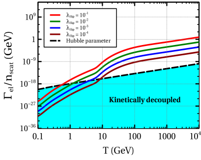
Figure 1: Variation of the elastic scattering rate ($\Gamma_{\rm el}$) normalised by $n_{\rm scat}$ with $T$ for different values of $\lambda_{H\phi}$ (left panel) and $M_{\phi}$ (right panel) respectively. Additionally, we have also shown the corresponding values of $\mathcal{H}(T)$ by the black dashed line for comparison.

The decoupling temperature $T_{\rm dec}$, beyond which $\phi$ can no longer be in kinetic equilibrium with the SM bath, is obtained approximately from $\dfrac{1}{n_{\rm scat}}\dfrac{\Gamma_{\rm el}}{\mathcal{H}}\bigg{|}_{\scriptsize T_{\rm dec}}\simeq 1$ Gorbunov:2011zz ; Gondolo:2012vh . Here, $\Gamma_{\rm el}=\sum_{X}n^{\rm eq}_{X}\times\langle\sigma{\rm v}\rangle_{\phi X\rightarrow\phi X}$ is the elastic scattering ($\phi X\rightarrow\phi X$) rate while $n^{\rm eq}_{X}$ being the equilibrium number density of the SM species $X$. The Hubble parameter controlling the expansion of the universe is denoted by $\mathcal{H}$. Moreover, the quantity $n_{\rm scat}\sim\frac{M_{\phi}}{T}$ represents the number of scatterings required so that the energy transfer between the SM bath and $\phi$ is $\sim T$ Gorbunov:2011zz . In Fig.  1, we have depicted how the quantity $\Gamma_{\rm el}/n_{\rm scat}$ varies with $T$ for four different values of the portal coupling $\lambda_{H\phi}$ and $M_{\phi}$ respectively. The expressions of necessary scattering cross sections are given in Appendix  B and the corresponding Feynman diagrams are shown in the lower panel of Fig.  2. Moreover, to understand the era of kinetic decoupling of $\phi$ we have also shown the variation of the Hubble parameter $\mathcal{H}(T)$ for the entire considered range $100\,\,{\rm MeV}\leq T\leq 10^{4}$ GeV. From the left panel of Fig.  1, we can see that the decoupling of $\phi$ occurs between $600\,\,{\rm MeV}\leq T_{\rm dec}\leq 10$ GeV for $M_{\phi}=100$ GeV and $0.1\geq\lambda_{H\phi}\geq 10^{-4}$. Similarly, the mass of $\phi$ also plays a crucial role in determining the decoupling temperature and that has been illustrated in the right panel where we have kept $\lambda_{H\phi}$ fixed at $10^{-3}$. In this case, for the increment of $M_{\phi}$ from 10 GeV to 250 GeV, the corresponding $T_{\rm dec}$ changes from 900 MeV to 4 GeV.

Therefore, we have two regimes separated by the decoupling temperature $T_{\rm dec}$. When $T\geq T_{\rm dec}$, all the dark sector species maintain kinetic equilibrium with the SM bath. Considering $\frac{Y_{i}}{Y}\simeq\frac{Y^{eq}_{i}}{Y^{eq}}$ ($i=\phi,\,\,\psi$) Griest:1990kh ; Edsjo:1997bg , we can reduce two coupled Boltzmann equations for $\phi$ and $\psi$ into a single equation involving the total comoving number density $Y=Y_{\phi}+Y_{\psi}$ i.e.

$$\dfrac{dY}{dx}=-\dfrac{1}{2}\dfrac{\beta\,{\rm s}}{\mathcal{H}\,x}\langle{\sigma{\rm v}}\rangle_{eff}\left[Y^{2}-(Y^{eq})^{2}\right]\,,$$ (12)

where, $x=\frac{M_{0}}{T}$ with $M_{0}$ being any arbitrary mass scale. Moreover, ${\rm s}$ is the entropy density of the universe and $\beta(T)=\dfrac{g^{1/2}_{\star}(T)\sqrt{g_{\rho}(T)}}{g_{s}(T)}$ with $g_{s}$ and $g_{\rho}$ being the effective DOFs associated with entropy and energy densities respectively while $g^{1/2}_{\star}=\dfrac{g_{s}}{\sqrt{g_{\rho}}}\left(1+\dfrac{1}{3}\dfrac{T}{g_{s}}\dfrac{dg_{s}}{dT}\right)$. Furthermore, the effective annihilation cross section $\langle{\sigma{\rm v}}\rangle_{eff}$ is given by

$$\langle{\sigma{\rm v}}\rangle_{eff}=\dfrac{\langle{\sigma{\rm v}}\rangle_{\phi\phi^{\dagger}\rightarrow X\overline{X},\,{\nu}_{R}\nu_{R}}\,(Y^{\rm eq}_{\phi})^{2}+\langle{\sigma{\rm v}}\rangle_{\psi\bar{\psi}\rightarrow{\nu}_{R}\nu_{R}}\,(Y^{\rm eq}_{\psi})^{2}}{\left(Y^{\rm eq}_{\phi}+Y^{\rm eq}_{\psi}\right)^{2}}\,.$$ (13)

Here, $\phi\phi^{\dagger}\rightarrow X\overline{X}$ represents the pair annihilations of $\phi$ and $\phi^{\dagger}$ into the SM species through the Higgs portal interaction and the expressions of such cross sections for a real scalar field are given in Guo:2010hq ; Biswas:2013nn .

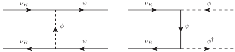
(a) Scatterings responsible for thermalisation of $\nu_{R}$ within the dark sector.

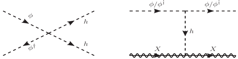
(b) Thermalisation processes of $\phi$ with the SM bath.

Figure 2: Feynman diagrams for the relevant scatterings. Here $X$ is any SM particles (fermion or boson).

On the other hand, for $T<T_{dec}$, although the dark sector has decoupled from the SM bath, they still maintains a local thermodynamic equilibrium among $\phi$, $\psi$ and $\nu_{R}$ with a common temperature $T_{\nu_{R}}\,(\neq T)$ due to sufficiently strong Yukawa coupling $y_{\phi}$. The kinetic equilibrium within the dark sector sustains well beyond the era of freeze-out by virtue of adequate elastic scatterings $\nu_{R}+\phi(\psi)\rightarrow\nu_{R}+\phi(\psi)$. However, besides $Y$, in this regime we need to solve an additional Boltzmann equation for the dark sector temperature $T_{\nu_{R}}$. Before writing these two Boltzmann equations, let us define a quantity $\xi=\dfrac{T_{\nu_{R}}}{T}$. In terms of three dimensionless quantities namely $Y$, $x$ and $\xi$, the Boltzmann equations for $Y$ and $\xi$ are given by

$$\dfrac{dY}{dx} = -\dfrac{1}{2}\dfrac{\beta\,{\rm s}}{\mathcal{H}\,x}\langle{\sigma{\rm v}}\rangle_{eff}\left[Y^{2}-(Y^{eq})^{2}\right]\,,$$ (14)

$$x\,\dfrac{d\xi}{dx}+(\beta-1)\xi = \dfrac{1}{2}\,\dfrac{\beta\,x^{4}\,{\rm s}^{2}}{4\,\alpha\,\xi^{3}\,\mathcal{H}\,M_{0}^{4}}\langle{E\sigma{\rm v}}\rangle_{eff}\left[Y^{2}-(Y^{eq})^{2}\right],$$ (15)

where,

$$\langle{E\sigma{\rm v}}\rangle_{eff}=\dfrac{(Y^{\rm eq}_{\psi})^{2}\langle{E\,\sigma{\rm v}}\rangle^{\prime}_{\nu_{R}\overline{\nu_{R}}\rightarrow\psi\overline{\psi}}\,+(Y^{\rm eq}_{\phi})^{2}\langle{E\,\sigma{\rm v}}\rangle^{\prime}_{\nu_{R}\overline{\nu_{R}}\rightarrow\phi\phi^{\dagger}}}{\left(Y^{eq}_{\phi}+Y^{eq}_{\psi}\right)^{2}}\,$$ (16)

and $\alpha=g_{\nu_{R}}\times\dfrac{7}{8}\dfrac{\,\,\pi^{2}}{30}$ with $g_{\nu_{R}}=2$. The difference between the two Boltzmann equations (Eqs. (12) and (14)) is that for $T\geq T_{\rm dec}$, $Y$, $Y^{eq}$ and $\langle{\sigma{\rm v}}\rangle_{eff}$ all are functions of $T$ (or $x$) only while in the later case when $T$ drops below $T_{\rm dec}$ all these quantities depend on both $x$ and $\xi$. The evolution of $\xi$ with respect to $x$ (equivalent to $T_{\nu_{R}}$ vs $T$) is described by Eq. (15) where similar to $\langle{\sigma{\rm v}}\rangle_{eff}$, the quantity $\langle{E\sigma{\rm v}}\rangle_{eff}$ also depends on both $x$ and $\xi$. A detail derivation of the Boltzmann equation for $\xi$ has been presented in Appendix A along with the definition of thermal average of $E\times\sigma{\rm v}$ for a process like $\nu_{R}\overline{\nu_{R}}\rightarrow j\bar{j}$. In Eq. (16) the prime over $\langle{E\sigma{\rm v}}\rangle_{\nu_{R}\overline{\nu_{R}}\rightarrow j\bar{j}}$ denotes thermal average of $E\times\sigma{\rm v}$ normalised by the product of equilibrium number densities of the final state particles $j$ and $\bar{j}$ respectively. The Feynman diagrams for the thermalisation of $\nu_{R}$ within the dark sector with $\psi$ and $\phi$ are shown in Fig. 2. Moreover, the same interactions (interchanging the initial and the final states) are involved in the freeze-out process of dark matter $\psi$. As a result we obtain strong constraint on dark matter phenomenology from the CMB bound on $\Delta{N}_{\rm eff}$ and it has been shown in Section V. Before going to the next section on $\Delta{N}_{\rm eff}$, we now discuss on the DM-nucleus scattering cross section in the remaining part of this section.

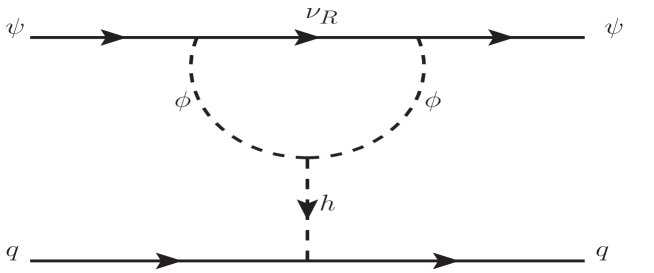
Figure 3: Feynman diagram for the scattering of $\psi$ at direct detection experiments.

Although our dark matter candidate does not have any direct coupling with the SM fields, it can still scatter off the detector nucleus efficiently depending on the portal coupling $\lambda_{H\phi}$, the new Yukawa coupling $y_{\phi}$ and the mass $M_{\psi}$. The scalar mediated spin independent DM-nucleon scattering occurs at one loop level, where the complex scalar $\phi$ and $\nu_{R}$ are running into the loop and the SM Higgs is playing the role of the mediator. The Feynman diagram of this scattering is shown in Fig. 3. The spin independent scattering cross section between $\psi$ and nucleon ($N$) is given by,

$$\sigma_{\rm SI}=\left(\dfrac{m_{N}}{v}\right)^{2}\,\dfrac{\mu_{\psi N}^{2}\,g_{\overline{\psi}\psi\,h}^{2}}{\pi\,m_{h}^{4}}\,f_{N}^{2}\,,$$ (17)

where, $\mu_{\psi\,N}=\frac{M_{\psi}m_{N}}{M_{\psi}+m_{N}}$ is the reduced mass of DM-nucleon system with $m_{N}$ being the mass of nucleon. The Higgs-nucleon coupling is proportional to the factor $f_{N}\simeq 0.3$ which depends on the quark content within a nucleon for each quark flavour Cline:2013gha . The effective vertex factor for the trilinear interaction vertex $\overline{\psi}\psi h$ is denoted by $g_{\overline{\psi}\psi\,h}$ and its expression in the low momentum transfer limit ($t<<M^{2}_{\psi}$) is given by,

$$g_{\overline{\psi}\,\psi\,h}=\frac{i}{16\pi^{2}}\times\frac{y_{\phi}^{2}\lambda_{H\phi}\,v}{M_{\psi}}\times\left[1+\left(\frac{M_{\phi}^{2}}{M_{\psi}^{2}}-1\right){\rm ln}\left(1-\frac{M_{\psi}^{2}}{M_{\phi}^{2}}\right)\right]\,.$$ (18)

We have computed the spin-independent scattering cross section using Eqs. ((17) and (18)) and have found the allowed parameter space after comparing with the latest data from XENON1T experiment Aprile:2018dbl in Section V.

IV Contribution to $N_{\rm eff}$ due to the Dirac nature of neutrinos

As we discussed earlier, we have considered one of the minimal extensions of the SM here to address the dark matter and light sub-eV scale Dirac neutrinos. As a result, the right chiral parts ($\nu_{R}$) are as light as the corresponding left chiral counterparts ($\nu_{L}$) and thus we are bound to get additional contributions to $N_{\rm eff}$. Consequently, the present bound on $\Delta{N_{\rm eff}}$ constrain the interaction strength of $\nu^{\alpha}_{R}$ and hence the decoupling from plasma prior to the onset of BBN. Most importantly, in the present case, $\nu^{\alpha}_{R}$ thermalises with the SM bath through its interaction with the complex scalar $\phi$ and the dark matter candidate $\psi$ as the sub-eV scale neutrino masses require the corresponding Yukawa couplings with the SM leptons and SM Higgs to be as minuscule as $\sim 10^{-12}$. The decoupling of $\nu^{\alpha}_{\rm R}$ is triggered as soon the kinetic equilibrium between $\phi$ and the SM bath is lost. Thereafter, all three $\mathbb{Z}_{4}$ odd species maintain a local thermal equilibrium among themselves by virtue of the new Yukawa interaction. As we have seen from Fig.  1, the kinetic decoupling of $\phi$ essentially depends on the portal coupling $\lambda_{H\phi}$ and the mass $M_{\phi}$. This results in a lower bound on the mass of dark matter indirectly as we need $M_{\psi}<M_{\phi}+m_{\nu}$ for a stable dark matter candidate $\psi$. Note that DM coupling to the SM neutrinos have been studied in the context of BBN and CMB constraints in earlier works, see Nollett:2014lwa for example. Typically sub-GeV thermal DM gets constrained from such bounds if they have sizeable couplings to SM neutrinos. As we will see in our work, DM with much heavier mass range ($M_{\psi}\geq 1$ GeV) can also be constrained if they have couplings with light Dirac neutrinos.

The additional contributions to $N_{\rm eff}$ at the time of CMB formation due to three right handed neutrinos can be obtained using the definition of $N_{\rm eff}$ (Eq. (1)) as

$$\Delta{N_{\rm eff}} = \dfrac{\sum_{\alpha}\varrho_{\nu^{\alpha}_{R}}}{\varrho_{\nu_{L}}}\,,$$ (19)

$$= 3\times\dfrac{\varrho_{\nu_{R}}}{\varrho_{\nu_{L}}}\,,$$

$$= 3\times\left(\dfrac{T_{\nu_{R}}}{T_{\nu_{L}}}\right)^{4}\bigg{|}_{T_{\rm CMB}}\,,$$

where $T_{\rm CMB}\simeq 0.26$ eV is the photon temperature at the time of the CMB formation. In the above, a couple of assumptions have been used. Firstly, we have made a simplifying assumption that all three right handed neutrinos have same couplings for the new Yukawa interaction and this makes the behaviour of all $\nu_{R}$s identical. Accordingly, we have substituted $\sum_{\alpha}\varrho_{\nu^{\alpha}_{R}}=3\times\varrho_{\nu_{R}}$ with $\varrho_{\nu_{R}}$ being the energy density of a single species of right handed neutrino. Moreover, we have used the equilibrium distribution function for the right handed neutrinos throughout its cosmological evolution. This is indeed the situation for a massless species (e.g. photon), which was once in equilibrium preserves its distribution function even after decoupling Dolgov:2002wy . The similar situation would be valid for a massive species like neutrinos if they decouple from the plasma containing $e^{\pm}$ and $\gamma$ instantly. In reality, this is not the case and hence spectral distortion in the distribution function is inevitable after decoupling. However, the amplitude of distortion is not much significant and for the left handed $\nu_{e}$ it has been shown in Dolgov:2002wy that $\left|\dfrac{\delta f}{f^{eq}_{\nu_{e}}}\right|\sim 10^{-4}$ for $E\sim T$ and $\delta f=f_{\nu_{e}}-f^{eq}_{\nu_{e}}$. Therefore, we have neglected this small distortion in the distribution function and consider $\varrho_{\nu_{R}}\propto T^{4}_{\nu_{R}}$ even after decoupling. Furthermore, for $T_{\nu_{R}}<<T_{dec}$ when the annihilation rate $\Gamma_{\nu^{\alpha}_{R}\overline{\nu^{\alpha}_{R}}\rightarrow j\bar{j}}<<\mathcal{H}$, the energy density of $\nu_{R}$ redshifts as $1/{a(t)}^{4}$ with $a(t)$ being the cosmic scale factor in the Friedmann-Lemaitre-Robertson-Walker (FLRW) metric. As a result, the ratio $T_{\nu_{R}}/T_{\nu_{L}}$ remains unaffected after the decoupling of $\nu_{L}$ as the temperature of $\nu_{L}$, after $T\sim 1$ MeV, behaves identically with the scale factor as that of $T_{\nu_{R}}$. Consequently, we do not need to compute the ratio of $T_{\nu_{R}}$ and $T_{\nu_{L}}$ at $T=T_{\rm CMB}$. Instead, the ratio evaluated at a much larger temperature i.e. just before the decoupling of $\nu_{L}$ ($T>T^{\rm dec}_{\nu_{L}}>>T_{\rm CMB}$) is sufficient to determine $\Delta{N_{\rm eff}}$ at $T_{\rm CMB}$. Therefore, one can rewrite the expression of $\Delta{N_{\rm eff}}$ in Eq. (19) as

$$\Delta{N_{\rm eff}} = 3\times\left(\dfrac{T_{{\nu}_{R}}}{T_{\nu_{L}}}\right)^{4}\bigg{|}_{T>T^{\rm dec}_{\nu_{L}}}\,,$$ (20)

$$= 3\times\left(\dfrac{T_{{\nu}_{R}}}{T}\right)^{4}\bigg{|}_{T>T^{\rm dec}_{\nu_{L}}}\,,$$

$$= 3\times\xi^{4}\bigg{|}_{T>T^{\rm dec}_{\nu_{L}}}\,,$$

where $\xi=\dfrac{T_{\nu_{R}}}{T}$ as defined earlier in Section III. In the last but one step, we have replaced $T_{\nu_{L}}$ by the photon temperature $T$ as before decoupling both $\nu_{L}$ and photon share a common temperature.

V Numerical Results

In this section we will present our numerical results. Our principal goal is to find the relic density of $\psi$ and the contribution of $\nu_{R}$s to $N_{\rm eff}$. As we have mentioned earlier that before the kinetic decoupling of $\phi$ ($T\geq T_{dec}$) from the SM bath, both the sectors have a common temperature and hence $\xi=1$. In this regime, to obtain the dark matter abundance we require to solve the Eq.  (12) only and it has been done using the package micrOMEGAs Belanger:2014vza , where the model information has been provided to micrOMEGAs using the package FeynRules Alloul:2013bka . The output of micrOMEGAs at $T=T_{\rm dec}$ has been used as an input for the second regime ($T<T_{\rm dec}$). In this regime, besides the Boltzmann equation for $Y$ given in Eq.  (14), we need to solve another Boltzmann equation for $\xi$ (or equivalently for $T_{\nu_{R}}$) also as here $T_{\nu_{R}}\neq T$. The Boltzmann equation describing the variation of $\xi$ with $x$ (inverse of $T$) is given in Eq.  (15). We have solved the two coupled differential equations numerically using our own codes. The expressions for relevant annihilation cross sections involving dark sector particles, which are required for solving Eq.  (14) and Eq.  (15) numerically, are given in Appendix C. The results are presented in Figs.  4-7.

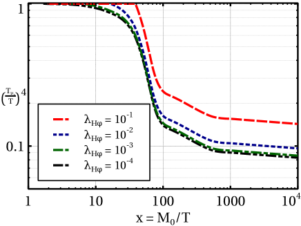
Figure 4: Variation of $\left(\frac{T_{\nu_{R}}}{T}\right)^{4}$ with $x$ for three different benchmark points such as $M_{\phi}=25$ GeV, $M_{\psi}=5$ GeV (the left plot in upper panel), $M_{\phi}=50$ GeV, $M_{\psi}=5$ GeV (the right plot in upper panel) and $M_{\phi}=250$ GeV, $M_{\psi}=5$ GeV (the plot in lower panel). In the upper panel $T$ varies between 10 GeV to 1 MeV while in the lower panel we have 100 GeV $\leq T\leq$ 1 MeV. Moreover, in all three plots we have kept the new Yukawa coupling $y_{\phi}$ fixed at $0.25$.

In Fig.  4 we have shown the variation of $\xi^{4}$ with $x$ for three different sets of dark sector particles masses. In this work we have fixed $M_{0}$ at 10 GeV. In the left plot at upper panel, we have depicted how $\xi^{4}$ changes with $x$ for $M_{\psi}=5$ GeV and $M_{\phi}=25$ GeV. In this plot we have considered four different values of portal couplings such as $\lambda_{H\phi}=10^{-1}$ (red dashed line), $10^{-2}$ (blue dotted line), $10^{-3}$ (green dash-dot line) and $10^{-4}$ (black dash-dot-dot line) respectively. One can clearly observe that the era at which deviation of $\xi$ from unity occurs gets delayed as we increase the portal coupling $\lambda_{H{\phi}}$. This is primarily due to the reason that the higher values of $\lambda_{H\phi}$ prolonged the kinetic equilibrium between the dark sector and the SM bath. For example, the point of deviation of $\xi$ from unity shifts from $x=40$ ($T=0.25$ GeV) to $x=2$ ($T=5$ GeV) when the portal coupling is decreased by three orders of magnitude from $\lambda_{H\phi}=10^{-1}$. Once $\xi$ departs from unity, it continues to decrease with $T$ and there is a sharp decrease of $\xi$ between $x\sim 10$ ($T\sim 1$ GeV) and $x\sim 100$ ($T\sim 100$ MeV). This happens mainly due to the term $\beta$ in the left hand side of Eq. (15), which is approximately equal to unity at very high and low temperatures and gets a peak at $T\sim 150$ MeV (around the QCD phase transition temperature) as all effective DOFs ($g_{\rho}$, $g_{s}$ and $g^{1/2}_{\star}$) diminish sharply during this period Husdal:2016haj .

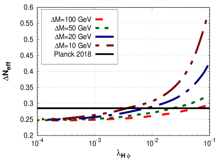
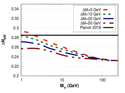
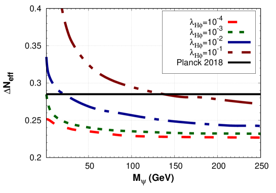
Figure 5: Variation of $\Delta{N}_{\rm eff}$ with relevant model parameters. The black solid line in each plot indicates the $2\sigma$ upper limit of $\Delta{N}_{\rm eff}$ ($\Delta{N}_{\rm eff}=0.285$) from the Planck 2018 data. In addition, all three plots are drawn for $y_{\phi}=0.2$ while the portal coupling $\lambda_{H\phi}=10^{-3}$ for the plot at top-right panel and the mass splitting $\Delta{M}=10$ GeV for the plot at the bottom panel respectively.

Thereafter, as $T$ reduces further and reaches up to a few MeV range, the quantity $\beta$ again revives to almost unity and $\xi$ becomes independent of $T$. Now, comparing plots for different $\lambda_{H\phi}$s we can conclude that a delayed kinetic decoupling leads to higher values of $\xi$ at $T=1$ MeV and hence a larger contribution to $N_{\rm eff}$ (automatically follows from Eq.  (20). The similar nature of $\xi$ has also been observed in the $\xi$ vs $x$ plots for other two benchmark points namely $M_{\phi}=50$ GeV, $M_{\psi}=5$ GeV (the right plot in upper panel) and $M_{\phi}=250$ GeV, $M_{\psi}=5$ GeV (the plot in lower panel) respectively. The only change we have noticed after comparing all three plots is that the scenario with smallest $M_{\phi}$ contributes maximally to $N_{\rm eff}$ as in this case $\phi$ maintains kinetic equilibrium up to a lowest possible temperature.

In Fig.  5, we demonstrate how $\Delta{N}_{\rm eff}$ varies with change in different model parameters. In all three plots we have considered $y_{\phi}=0.2$. In the top-left plot of Fig.  5, we have shown the dependence of $\Delta{N}_{\rm eff}$ on the portal coupling $\lambda_{H\phi}$. This plot has been drawn for four different values of mass splitting $\Delta{M}=10$ GeV, 20 GeV, 50 GeV and 100 GeV respectively between $\phi$ and $\psi$. Similar to the previous plots of $\xi$ in Fig.  4, here also we observe the same nature of $\Delta{N}_{\rm eff}$ with respect to $\lambda_{H\phi}$ and $\Delta{M}$. We find that $\Delta{N}_{\rm eff}$ behaves oppositely with respect these two parameters. The contribution to $N_{\rm eff}$ due to three right handed neutrinos enhances sharply as we increase $\lambda_{H\phi}$ further however, the large mass splitting between dark matter and $\phi$ reduces the effect of $\nu_{R}$s on $N_{\rm eff}$.

The effect of dark sector particle masses on $\Delta{N}_{\rm eff}$ will be more understandable from the second plot in the top-right panel of Fig.  5 where we have illustrated the variation of $\Delta{N}_{\rm eff}$ with $M_{\phi}$ for four different values of mass splitting $\Delta{M}=5$ GeV, 10 GeV, 20 GeV and 50 GeV respectively. This plot is generated for $\lambda_{H\phi}=10^{-3}$. It is clearly seen from this plot that $\Delta{N}_{\rm eff}$ rises as we lower $M_{\psi}$ from 100 GeV to 1 GeV. Moreover, comparing the red dashed line for $\Delta{M}=5$ GeV and the brown dash-dot-dot line for $\Delta{M}=50$ GeV, one can easily conclude that lower mass splitting produces larger $\Delta{N}_{\rm eff}$. In some cases, e.g. for $\Delta{M}=5$ GeV and $M_{\psi}\lesssim$ 2 GeV, the contribution of three $\nu_{R}$s even overshoots the $2\sigma$ upper bound from the Planck 2018 data while other scenarios are still viable. Nevertheless, $\Delta{N}_{\rm eff}$ becomes insensitive to both these parameters beyond $M_{\psi}\sim 100$ GeV where all four curves are almost parallel to the X axis. This is consistent with the approximate calculation of $\Delta{N}_{\rm eff}$ using entropy conservation where the contribution of a relativistic species to $N_{\rm eff}$ saturates if it decouples well above $T\sim 100$ GeV Abazajian:2019oqj .

Finally, in the third plot at the bottom panel, we have depicted the combined effects of $M_{\psi}$ and $\lambda_{H\phi}$ on $\Delta{N}_{\rm eff}$. This plot has been generated for $\Delta{M}=10$ GeV. From this plot it is clearly seen that the entire considered mass range of $\psi$ i.e. $1\,\,{\rm GeV}\leq M_{\psi}\leq 250$ GeV is allowed by the Planck 2018 data for $\lambda_{H\phi}\leq 10^{-3}$. However, for $\lambda_{H\phi}\geq 10^{-3}$ the low mass region of $\psi$ is already ruled out, e.g. when $\lambda_{H\phi}=10^{-2}$ and $10^{-1}$, the mass $M_{\psi}$ up to 20 GeV and 135 GeV respectively are excluded by the $2\sigma$ upper limit of $\Delta{N}_{\rm eff}$.

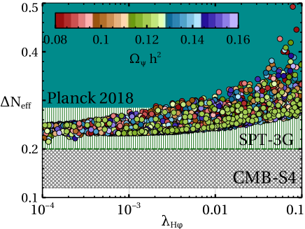
(a) Variation of $\Delta{N}_{\rm eff}$ with $\lambda_{H\phi}$

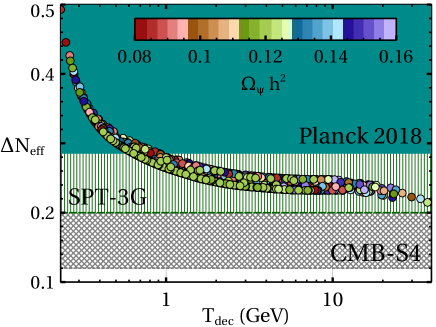
(b) Variation of $\Delta{N}_{\rm eff}$ with $T_{dec}$

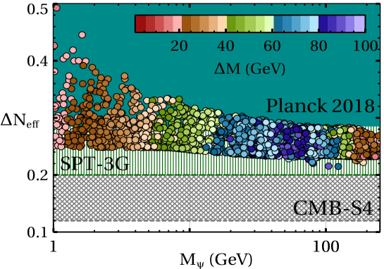
(c) Variation of $\Delta{N}_{\rm eff}$ with $M_{\psi}$

Figure 6: All three plots are generated by varying the model parameters in the range as mentioned in Eq.  (24). In each plot the dark cyan region is the current $2\sigma$ upper limit on $\Delta{N_{\rm eff}}$ from the Planck 2018 data while sensitivities of the two upcoming CMB experiments are also presented for comparison.

To understand the entire picture in a well organised manner we have shown our parameter space allowed from both dark matter relic density constraint and the bound on $\Delta{N}_{\rm eff}$ in Fig.  6. In order to obtain the parameter space we have varied our model parameters in the following range

$$\begin{array}[]{cccccc}10^{-4}&\leq&\lambda_{H\phi}&\leq&10^{-1}\,\,,\\ 1.0\,\,{\rm GeV}&\leq&M_{\psi}&\leq&250.0\,\,{\rm GeV}\,\,,\\ 1.0\,\,{\rm GeV}&\leq&\Delta{M}&\leq&100.0\,\,{\rm GeV}\,\,,\end{array}$$ (24)

while the new Yukawa coupling $y_{\phi}$ has been kept fixed 0.2. In the top-left panel of Fig.  6, we have demonstrated $\Delta{N_{\rm eff}}$ vs $\lambda_{H\phi}$ parameter space where the remaining parameters are varied according to Eq.  24. The relic density of dark matter candidate $\psi$ has been indicated by the colour bar where the current $3\sigma$ range of $\Omega_{\psi}h^{2}$ ($0.1170\leq\Omega_{\psi}h^{2}\leq 0.1230$) falls within the green coloured patch. Additionally, the present $2\sigma$ upper bound on $\Delta{N}_{\rm eff}$ from the Planck 2018 data is shown by the dark cyan coloured region while the sensitivities of two upcoming CMB experiments namely SPT-3G Avva:2019hzz and CMB-S4 Abazajian:2016yjj have also been indicated by green vertical lines and gray cross lines respectively. From this plot we observe that although the relic density of dark matter satisfies the current bound for the entire considered range of $\lambda_{H\phi}$, the Planck limit on $\Delta{N}_{\rm eff}$ excludes some portion of the parameter space for higher values of the portal coupling i.e. $\lambda_{H\phi}\geq 2\times 10^{-3}$. Nevertheless, the remaining entire parameter space will be probed by the upcoming experiments.

In the top-right panel of Fig.  6, we show how $\Delta_{N_{\rm eff}}$ changes when the decoupling temperature of $\phi$ from the SM bath varies between 200 MeV to 30 GeV. The variation of $T_{\rm dec}$ is due to corresponding variation of $\Delta{M}$, $M_{\psi}$ and $\lambda_{H\phi}$ in the full range as given in Eq.  (24). This plot clearly reveals that scenarios where three right handed neutrinos remain thermalised with the SM bath as late as up to $T=800$ MeV are still allowed while scenarios with $T_{\rm dec}<600$ MeV are completely ruled out for producing excess contribution to $N_{\rm eff}$. This is quite consistent with earlier result of Ref.  Abazajian:2019oqj . Moreover, in the intermediate range where $T_{\rm dec}$ lies between 800 MeV to 600 MeV are partially allowed depending on the values of relevant parameters namely $\Delta{M}$, $M_{\psi}$ and $\lambda_{H\phi}$. In the bottom panel we have presented $\Delta{N}_{\rm eff}$ vs $M_{\psi}$ parameter space, where the mass of other dark sector particle $\phi$ has been indicated in terms of $\Delta{M}$ using colour bar. From this plot one can easily notice that an enhanced effect of $\nu_{R}$s to $N_{\rm eff}$ is obtained for smaller values of $M_{\psi}$ and $\Delta{M}$. Moreover, here also some portion of parameter space is already excluded by the Planck 2018 data and the remaining parameter space is well within the reach of upcoming experiments.

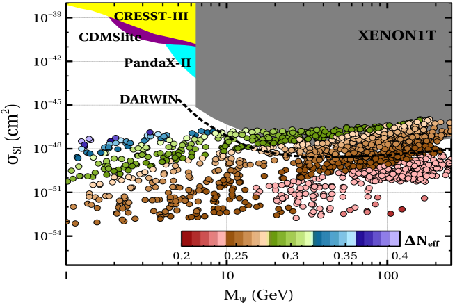
Figure 7: Comparison of spin independent scattering cross section of $\psi$ obtain from the present model with existing as well as projected bounds from various direct detection experiments. All the points in $\sigma_{\rm SI}-M_{\psi}$ plane satisfy relic density bound in $3\sigma$ range i.e. $0.117\leq\Omega_{\psi}h^{2}\leq 0.123$. The colour bar indicates corresponding values of $\Delta{N}_{\rm eff}$.

As we already mentioned, our dark matter candidate $\psi$ has no direct coupling with the SM fields. Nevertheless, $\psi$ can still scatter off the detector nucleus at radiative level and thereby it may produce observable signal at the direct detection experiments. The scattering occurs at one loop level as shown in Fig.  3. We have computed the spin independent elastic scattering $\psi N\rightarrow\psi N$ using the expression of $\sigma_{\rm SI}$ given in Eq.  (17). The result is shown in Fig.  7. Moreover, to compare our result with the existing experimental upper bounds on spin independent dark matter-nucleon cross sections, we have shown upper limits from XENON1T Aprile:2018dbl , PandaX-II Tan:2016zwf , CDMSlite Agnese:2017jvy and CRESST-III Abdelhameed:2019hmk experiments in the same plot. We find that in spite of being a loop suppressed scattering process, the high dark matter mass region ($M_{\psi}>10$ GeV) is being probed by XENON1T experiment and it has already excluded a small portion of the parameter space. Moreover, most of the excluded parameter space is also disallowed by the $2\sigma$ upper limit on $\Delta{N}_{\rm eff}$ from the Planck 2018 data. The future direct detection experiment like DARWIN Aalbers:2016jon (projected limit has been shown by the black dashed line) will have the sensitivity to probe the remaining parameter space in the high mass region which is still allowed by the $2\sigma$ bound on $\Delta{N}_{\rm eff}$ and lying just above the “neutrino-floor”, a region dominated by the coherent elastic neutrino-nucleus scattering. However, for the lighter dark matter masses ($M_{\psi}\lesssim 10$ GeV) the present direct detection experiments are not sensitive enough and thus the entire relic density satisfied parameter space (in $3\sigma$ range), in this regime, remains far beyond the reach of current and upcoming experiments as well. Nonetheless, the low mass region is extremely sensitive to be probed by the CMB experiments measuring $N_{\rm eff}$. From this plot, one can easily notice that some of the allowed parameter space in $\sigma_{\rm SI}-M_{\psi}$ plane where $\sigma_{\rm SI}$ is as low as $\sim 10^{-48}$ cm² to $\sim 10^{-50}$ cm² depending on $M_{\psi}$ (blue, cyan and green coloured points) has already been ruled out by the current $2\sigma$ upper bound on $\Delta{N}_{\rm eff}$. The remaining parameter space for the entire considered range of $M_{\psi}$ is well within the sensitivities of the upcoming CMB experiments like CMB-S4 Abazajian:2016yjj , SPT-3G Benson:2014qhw , Simons Observatory Ade:2018sbj etc. Therefore, these next generation CMB experiments will be able to either validate or falsify this kind of neutrino portal dark matter scenario in very near future.

We would like to note in passing that although in this minimal model we require extremely tiny Yukawa coupling $\sim 10^{-12}$ for obtaining sub-eV scale Dirac neutrino masses, such fine-tuning can be avoided by introducing another scalar doublet $H_{2}$ with an induced VEV $v_{2}$ which could in principle be much lower than GeV scale. In this case, by suitably rearranging the $\mathbb{Z}_{4}$ charges, one can easily forbid the Dirac mass term involving the SM Higgs doublet while the Yukawa interaction involving $H_{2}$ with coupling $y_{H_{2}}$ is still allowed. Therefore, due to the induced VEV $v_{2}$, sub-eV scale Dirac mass of neutrinos can be generated for much larger Yukawa coupling $y_{H_{2}}$. As a result, besides the interaction with $\phi$, now $\nu_{R}$ can also thermalise with the SM plasma via scatterings with leptons like $\overline{\nu_{R}}\nu_{R}\rightarrow e^{+}e^{-},\overline{\nu_{L}}\nu_{L}$. However, the impact of that interaction will be significant which keeps $\nu_{R}$s in thermal equilibrium up to a smallest temperature.

VI Conclusion

We have proposed a scenario where dark matter interacts with the Standard Model particles only via light Dirac neutrinos, leading to a Dirac neutrino portal dark matter scenario. In a minimal setup, this requires the extension of the SM by three right handed neutrinos, one singlet Dirac fermionic DM ($\psi$) and one singlet complex scalar ($\phi$) to assist the coupling of DM with right handed neutrinos through a new Yukawa type interaction. The right handed neutrinos couple to the SM neutrinos via usual Yukawa interaction involving the SM Higgs doublet and acquire sub-eV scale Dirac masses by appropriate tuning of the corresponding Yukawa couplings. An additional $\mathbb{Z}_{4}$ symmetry is introduced for stabilising the dark matter candidate ($\psi$) and at the same time forbidding the unwanted Majorana mass of each $\nu_{R}$. The complex scalar $\phi$ thermalises with the SM bath through a portal coupling $\lambda_{H\phi}$ with the SM Higgs boson while both DM and $\nu_{R}$s maintain kinetic equilibrium with the SM plasma by virtue of the new Yukawa interaction involving $\psi$, $\nu_{R}$ and $\phi$. This leads to additional thermalised relativistic degrees of freedom in the early universe. Hence, the right handed neutrinos must de decoupled from the SM bath well before the decoupling era of their left handed counterparts, otherwise there would be too much contribution to $N_{\rm eff}$ due to three ${\nu_{R}}$s. The decoupling of $\nu_{R}$ occurs as the kinetic equilibrium between $\phi$ and the SM bath is lost. Subsequently $\psi$, $\phi$ and $\nu_{R}$s form a dark sector where all three species maintain an equilibrium among themselves with a common temperature $T_{\nu_{R}}$. The era of decoupling depends mostly on two parameters namely the portal coupling $\lambda_{H\phi}$ and the mass of $\phi$.

In order to find out the relic density of $\psi$ and $\Delta{N}_{\rm eff}$ we have solved numerically two coupled Boltzmann equations, one for the comoving density $Y$ and the rest is for $T_{\nu_{R}}$. After computing the relic density of $\psi$, we have calculated the spin independent elastic scattering cross section ($\sigma_{\rm SI}$) between $\psi$ and nucleon occurring at one loop level and mediated by the SM Higgs boson. We have found that a small portion of the high mass region ($M_{\psi}>10$ GeV) of our model is ruled out by the current exclusion limit on $\sigma_{\rm SI}$ from the XENON1T experiments. Interestingly, most of this region is also excluded from the present $2\sigma$ upper bound on $\Delta{N}_{\rm eff}$. The proposed direct detection experiment DARWIN will be able to probe the entire parameter space above the “neutrino-floor”. On the other hand, in the low mass regime as the sensitivity of direct detection experiments become less, our relic density satisfied parameter space remains very far to be probed directly by the current as well as upcoming experiments. However, in the low mass regime ($M_{\psi}\lesssim 10$ GeV), depending on $\Delta{M}$ and $\lambda_{H\phi}$, we already have some portion of the parameter space where $\nu_{R}$ remains in the thermal bath as late as $T\leq 600$ MeV and thereby producing excess contribution to $\Delta{N}_{\rm eff}$. This part of the parameter space is thus excluded by the current $2\sigma$ upper limit $\Delta{N_{\rm eff}}\leq 0.285$ from the Planck 2018 data. The next generation CMB experiments like CMB-S4, SPT-3G, Simons Observatory etc. will be sensitive enough to validate/falsify the present model by probing the entire dark matter mass region. Therefore, although the present direct detection experiments are not efficient enough in the low mass regime, such low mass dark matter scenarios can still be probed by measuring $\Delta{N}_{\rm eff}$ and for certain ranges of model parameters some part of the parameter space in low mass regime is already excluded where $\sigma_{\rm SI}$ is as low as $\sim 10^{-48}$ cm² to $\sim 10^{-50}$ cm². While this scenario offers a complementary way of probing such light DM scenarios via future CMB experiments, the active direct search strategies for low mass DM may also compete CMB experiments in near future. Additionally, possible UV completions of such minimal scenarios will also offer richer phenomenology and possibilities of linking DM and Dirac neutrinos to other problems in particle physics and cosmology (see He:2020zns for example). We leave a detailed discussion of such possibilities to future studies.

VII Acknowledgements

One of the authors AB would like to thank Sougata Ganguly for very useful discussions at various stages of this work. He also acknowledges the cluster computing facility at IACS (pheno-server).   DB acknowledges the support from Early Career Research Award from DST-SERB, Government of India (reference number: ECR/2017/001873). DN would like to acknowledge Lopamudra Mukherjee for a discussion regarding loop-induced scattering cross section.

Appendix A Derivation of the Boltzmann equation expressing evolution of $T_{\nu_{R}}$

In this appendix we will present a detail derivation of the temperature Boltzmann equation. Our starting point will be the total time derivative of the phase space distribution function $f_{A}(p,\,t)$ of a species ${\bf A}$ is equal to the Collision term including all possible interactions of ${\bf A}$ i.e.

$$\dfrac{d}{dt}f_{\bf A}(p,\,t)=\mathcal{C}[f_{\bf A}(p,\,t)]\,$$ (25)

where $p$ is the magnitude of three momentum $\vec{p}$ of the species ${\bf A}$. Since the linear momentum of species red-shifted as $a^{-1}$ due to the expansion of the universe, where $a$ is the scale factor of the FLRW metric, we have $\dfrac{\dot{p}}{p}=-\dfrac{\dot{a}}{a}=\mathcal{H}$. Using this relation, the LHS of the Eq. (25) can be written as

$$\left(\dfrac{\partial}{\partial t}-\mathcal{H}\,p\dfrac{\partial}{\partial p}\right)f_{\bf A}(p,\,t)=\mathcal{C}[f_{\bf A}(p,\,t)]\,.$$ (26)

The quantity within bracket in the above is proportional to the Liouville operator for the FLRW metric. Now, consider a specific interaction like ${\bf A}(\vec{p}_{1})+B(\vec{p}_{2})\rightarrow C(\vec{p}_{3})+D(\vec{p}_{4})$, where $\vec{p}_{i}$s are the three momenta and the corresponding energies are $E_{i}$s. We want to calculate the moment of an operator $\mathcal{O}(p_{1})$ for the species ${\bf A}$. This can be written as

$$\int\dfrac{g_{1}\,d^{3}\vec{p}_{1}}{(2\pi)^{3}}\left[\left(\dfrac{\partial}{\partial t}-\mathcal{H}\,p_{1}\dfrac{\partial}{\partial p_{1}}\right)f_{\bf A}(p_{1},\,t)\right]\mathcal{O}(p_{1}) = \int\dfrac{g_{1}\,d^{3}\vec{p}_{1}}{(2\pi)^{3}}\,\mathcal{C}[f_{\bf A}(p_{1},\,t)]\,\mathcal{O}(p_{1})\,.$$ (27)

Here $g_{1}$ is the internal degrees of freedom of ${\bf A}$. Assuming $f_{A}$ vanishes at the boundary, the LHS of the above equation can be further simplified as

$$\dfrac{d}{dt}\langle\mathcal{O}(p_{1})\rangle+3\mathcal{H}\left(\langle\mathcal{O}(p_{1})\rangle+\langle\dfrac{p_{1}}{3}\,\dfrac{\partial}{\partial p_{1}}\mathcal{O}(p_{1})\rangle\right)=\int\prod_{\alpha=1}^{4}d\Pi_{\alpha}\,\left(2\pi\right)^{4}\delta^{4}\left({\bf p}_{1}+{\bf p}_{2}-{\bf p}_{3}-{\bf p}_{4}\right)\times$$

$$~{}~{}~{}~{}~{}~{}~{}~{}~{}~{}~{}~{}~{}~{}~{}~{}~{}~{}~{}~{}~{}~{}\overline{\left|\mathcal{M}\right|}^{2}_{{\bf A}+B\rightarrow C+D}\left[f_{C}(p_{3},t)f_{D}({p}_{4},t)-f_{\bf A}({p}_{1},t)f_{B}({p}_{2},t)\right]\mathcal{O}(p_{1})\,\,,$$ (28)

where

$$\langle\mathcal{O}(p_{1})\rangle=\int d\Pi_{1}\,2E_{1}\,f_{\bf A}({p_{1}},\,t)\,\mathcal{O}(p_{1})\,.$$ (29)

with $d\Pi_{i}=\dfrac{g_{i}\,d^{3}\vec{p}_{i}}{(2\pi)^{3}\,2E_{i}}$ a Lorentz invariant phase space measure while ${\bf p_{i}}$ denotes the four momentum corresponding to energy $E_{i}$ and three momentum $\vec{p}_{i}$. Moreover, $\overline{\left|\mathcal{M}\right|}^{2}_{{\bf A}+B\rightarrow C+D}$ is the Lorentz invariant matrix element square averaged over both initial and final states spins. As we want to find the evolution of temperature of a species, therefore, in the present case $\mathcal{O}=E_{1}$. Thus, using Eq. (29) we have $\langle\mathcal{O}\rangle=\langle E_{1}\rangle=\rho_{\bf A}$ and $\langle\dfrac{p_{1}}{3}\,\dfrac{\partial}{\partial p_{1}}\mathcal{O}\rangle=\langle\dfrac{p^{2}_{1}}{3\,E_{1}}\rangle=P_{\bf A}$, the energy density and the pressure of $\bf A$ respectively. In terms of $\rho_{\bf A}$ and $P_{\bf A}$ the LHS of Eq. (28) takes the familiar form,

$$\dfrac{d}{dt}\rho_{\bf A}+3\mathcal{H}\left(\rho_{\bf A}+P_{\bf A}\right)=\int\prod_{\alpha=1}^{4}d\Pi_{\alpha}\,\left(2\pi\right)^{4}\delta^{4}\left({\bf p}_{1}+{\bf p}_{2}-{\bf p}_{3}-{\bf p}_{4}\right)\times$$

$$~{}~{}~{}~{}~{}~{}~{}~{}~{}~{}~{}~{}~{}~{}~{}~{}~{}~{}~{}~{}~{}~{}\overline{\left|\mathcal{M}\right|}^{2}_{{\bf A}+B\rightarrow C+D}\left[f_{C}(p_{3},t)f_{D}({p}_{4},t)-f_{\bf A}({p}_{1},t)f_{B}({p}_{2},t)\right]\,E_{1}\,\,.$$ (30)

The RHS of the above equation can be simplified in terms of the cross section $\sigma$ of the process ${\bf A}+B\rightarrow C+D$. Considering equilibrium distribution function as the Maxwell-Boltzmann distribution function, one can write the out of equilibrium distribution function of a species $\kappa$ having energy $E_{\kappa}$ and temperature $T^{\prime}$ as $f_{\kappa}=\dfrac{n_{\kappa}}{n^{eq}_{\kappa}}\exp(-\frac{E_{\kappa}}{T^{\prime}})$, where $n_{\kappa}$ is the number density of $\kappa$ and the equilibrium number density is $n^{eq}_{\kappa}$. Therefore, the RHS of Eq. (30) can be further simplified as

$$\dfrac{d}{dt}\rho_{\bf A}+3\mathcal{H}\left(\rho_{\bf A}+P_{\bf A}\right) = \left[\int\prod_{\beta=1}^{2}\dfrac{g_{\beta}\,d^{3}\vec{p}_{\beta}}{(2\pi)^{3}}\Bigg{\{}\dfrac{1}{4\,E_{1}\,E_{2}}\int\prod_{\alpha=3}^{4}d\Pi_{\alpha}\,\left(2\pi\right)^{4}\delta^{4}\left({\bf p}_{1}+{\bf p}_{2}-{\bf p}_{3}-{\bf p}_{4}\right)\right.\times$$

$$\left.\overline{\left|\mathcal{M}\right|}^{2}_{{\bf A}+B\rightarrow C+D}\Bigg{\}}E_{1}\,\exp\left(-\frac{E_{1}+E_{2}}{T^{\prime}}\right)\right]\left(\dfrac{n_{C}}{n^{eq}_{C}}\dfrac{n_{D}}{n^{eq}_{D}}-\dfrac{n_{\bf A}}{n^{eq}_{\bf A}}\dfrac{n_{B}}{n^{eq}_{B}}\right),$$

$$= \left[\int\prod_{\beta=1}^{2}\dfrac{g_{\beta}\,d^{3}\vec{p}_{\beta}}{(2\pi)^{3}}\,E_{1}\,\exp\left(-\frac{E_{1}+E_{2}}{T^{\prime}}\right)\sigma_{{\bf A}+B\rightarrow C+D}\right]\left(\dfrac{n_{C}}{n^{eq}_{C}}\dfrac{n_{D}}{n^{eq}_{D}}-\dfrac{n_{\bf A}}{n^{eq}_{\bf A}}\dfrac{n_{B}}{n^{eq}_{B}}\right)$$

$$= \langle E\,\sigma{\rm v}\rangle_{{\bf A}+B\rightarrow C+D}\left(n^{eq}_{\bf A}n^{eq}_{B}\dfrac{n_{C}}{n^{eq}_{C}}\dfrac{n_{D}}{n^{eq}_{D}}-n_{\bf A}{n_{B}}\right)\,.$$ (32)

Where, the cross section $\sigma_{{\bf A}+B\rightarrow C+D}$ is denoted by the curly bracket in Eq. (A) while the thermal average of $E\times\sigma{\rm v}$ is defined as

$$\langle E\,\sigma{\rm v}\rangle_{{\bf A}+B\rightarrow C+D}=\dfrac{1}{n^{eq}_{\bf A}n^{eq}_{B}}\int\prod_{\beta=1}^{2}\dfrac{g_{\beta}\,d^{3}\vec{p}_{\beta}}{(2\pi)^{3}}\,E_{1}\,\exp\left(-\frac{E_{1}+E_{2}}{T^{\prime}}\right)\sigma_{{\bf A}+B\rightarrow C+D}\,.$$ (33)

The expression of $\langle E\,\sigma{\rm v}\rangle_{{\bf A}+B\rightarrow C+D}$ can be further simplified by changing variables from $E_{1}$, $E_{2}$ and the angle $\theta$ between the initial state particles to $E_{\pm}=E_{1}\pm E_{2}$ and the Mandelstam variable $s$ respectively as given in Gondolo:1990dk . In this case, the integration limits for these newly defined variables are

$$\left|E_{-}-E_{+}\omega\right|\leq\sqrt{\dfrac{\Lambda(s,m^{2}_{\bf A},m^{2}_{B})}{s^{2}}}\sqrt{E^{2}_{+}-s}\,,$$ (34)

$$E_{+}\geq\sqrt{s}\,,$$ (35)

$$s\geq(m_{\bf A}+m_{B})^{2}\,,$$ (36)

where, the function $\Lambda(a,b,c)=(a-b-c)^{2}-4bc$ and $\omega=\dfrac{m^{2}_{\bf A}-m^{2}_{B}}{s}$ (assuming $m_{\bf A}\geq m_{B}$). Thereafter, following the procedure given in Gondolo:1990dk , the six dimension integration in Eq.  (33) reduces to an one dimensional integration on the Mandelstam variable $s$ as

$$\langle E\,\sigma{\rm v}\rangle_{{\bf A}+B\rightarrow C+D}=\dfrac{g_{\bf A}g_{B}}{n^{eq}_{\bf A}n^{eq}_{B}}\times\dfrac{T^{\prime}\,\pi^{2}}{(2\pi)^{6}}\int_{(m_{\bf A}+m_{B})^{2}}^{\infty}\sigma_{{\bf A}+B\rightarrow C+D}\,\Lambda(s,m^{2}_{\bf A},m^{2}_{B})\,(1+\omega)\,{\rm K}_{2}\left(\frac{\sqrt{s}}{T^{\prime}}\right)\,ds\,.$$

The equilibrium number density of a species $j$ obeying the Maxwell-Boltzmann distribution and having mass $m_{j}$, internal degrees of freedom $g_{j}$ and temperature $T^{\prime}$ is given by

$$n^{eq}_{j}(T^{\prime})=\dfrac{g_{j}\,T^{\prime}}{2\pi^{2}}m^{2}_{j}\,{\rm K}_{2}\left(\frac{m_{j}}{T^{\prime}}\right)\,.$$ (38)

Here, ${\rm K}_{2}\left(\frac{m_{i}}{T^{\prime}}\right)$ is the modified Bessel function of second kind. Therefore, if the initial state particles have same masses i.e. $m_{\bf A}=m_{B}=m$, the above expression of $\langle E\,\sigma{\rm v}\rangle$ reduces to the following simpler form,

$$\langle E\,\sigma{\rm v}\rangle_{{\bf A}+B\rightarrow C+D}=\dfrac{1}{16\,T^{\prime}m^{4}\,\left({\rm K}_{2}\left(\frac{m}{T^{\prime}}\right)\right)^{2}}\int_{4m^{2}}^{\infty}\sigma_{{\bf A}+B\rightarrow C+D}\,s\,(s-4m^{2})\,{\rm K}_{2}\left(\frac{\sqrt{s}}{T^{\prime}}\right)\,ds\,.$$ (39)

Moreover, during the derivation of Eq. (32) we have considered same temperature $T^{\prime}$ for all four species $\bf A$, $B$, $C$ and $D$. However, if the initial and the final states particles have different temperature namely $T_{i}$ and $T_{f}$ with $T_{i}\neq T_{f}$ then the Boltzmann equation of $\rho_{A}$ is given by

$$\dfrac{d}{dt}\rho_{\bf A}+3\mathcal{H}\left(\rho_{\bf A}+P_{\bf A}\right) = \langle E\,\sigma{\rm v}\rangle_{{\bf A}+B\rightarrow C+D}^{T_{f}}\,\,n^{eq}_{\bf A}(T_{f})n^{eq}_{B}(T_{f})\dfrac{n_{C}(T_{f})}{n^{eq}_{C}(T_{f})}\dfrac{n_{D}(T_{f})}{n^{eq}_{D}(T_{f})}$$ (40)

$$-\langle E\,\sigma{\rm v}\rangle_{{\bf A}+B\rightarrow C+D}^{T_{i}}\,\,n_{\bf A}(T_{i}){n_{B}}(T_{i})\,.$$

One can easily check that the RHS of the above equation reduces to Eq. (32) for $T_{i}=T_{f}=T^{\prime}$.

Before going to the specific case of the present model, we would like to discuss the possible effect of a decay process like ${B}(\vec{p}_{1})\rightarrow{\bf A}(\vec{p}_{2})+C(\vec{p}_{3})$ to the evolution of $\rho_{\bf A}$. The collision term contributing to the evolution of $\rho_{\bf A}$ due to this decay has the following form,

$$\mathcal{C}_{B\rightarrow{\bf A}+C} = \int\prod_{\alpha=1}^{3}d\Pi_{\alpha}\,\left(2\pi\right)^{4}\delta^{4}\left({\bf p}_{1}-{\bf p}_{2}-{\bf p}_{3}\right)\overline{\left|\mathcal{M}\right|}^{2}_{{B\rightarrow{\bf A}+C}}\left[f_{B}({p}_{1},t)-f_{\bf A}(p_{2},t)f_{C}({p}_{3},t)\right]\,E_{2}\,\,,$$ (41)

$$= \left(\dfrac{n_{B}}{n^{eq}_{B}}-\dfrac{n_{\bf A}}{n^{eq}_{\bf A}}\dfrac{n_{C}}{n^{eq}_{C}}\right)\int\prod_{\alpha=1}^{3}d\Pi_{\alpha}\,\left(2\pi\right)^{4}\delta^{4}\left({\bf p}_{1}-{\bf p}_{2}-{\bf p}_{3}\right)\overline{\left|\mathcal{M}\right|}^{2}_{{B\rightarrow{\bf A}+C}}\times$$

$$~{}~{}~{}~{}~{}~{}~{}~{}~{}~{}~{}~{}~{}~{}~{}~{}~{}~{}~{}~{}~{}E_{2}\exp\left(-\frac{E_{2}+E_{3}}{T^{\prime}}\right)\,.$$

Here we have assumed CP invariance as we did earlier in Eq.  (28). In the last step we have used the Maxwell-Boltzmann distribution function for all the species. Now, rearranging the collision term one can write it as

$$\mathcal{C}_{B\rightarrow{\bf A}+C} = \left(\dfrac{n_{B}}{n^{eq}_{B}}-\dfrac{n_{\bf A}}{n^{eq}_{\bf A}}\dfrac{n_{C}}{n^{eq}_{C}}\right)\int\prod_{\alpha=2}^{3}d\Pi_{\alpha}\,E_{2}\exp\left(-\frac{E_{2}+E_{3}}{T^{\prime}}\right)\times$$ (42)

$$~{}~{}~{}~{}~{}~{}~{}~{}\left\{\int d\Pi_{1}\left(2\pi\right)^{4}\delta^{4}\left({\bf p}_{1}-{\bf p}_{2}-{\bf p}_{3}\right)\overline{\left|\mathcal{M}\right|}^{2}_{B\rightarrow{\bf A}+C}\right\}\,.$$

The term within the curly brackets is Lorentz invariant and hence, can be evaluated in any inertial frame of reference. The most convenient is to calculate this term in the centre of momentum frame where

$$\int d\Pi_{1}\left(2\pi\right)^{4}\delta^{4}\left({\bf p}_{1}-{\bf p}_{2}-{\bf p}_{3}\right)\overline{\left|\mathcal{M}\right|}^{2}_{B\rightarrow{\bf A}+C}=\dfrac{g_{B}\,\pi}{m_{B}}\,\delta(\sqrt{s}-m_{B})\,\overline{\left|\mathcal{M}\right|}^{2}_{B\rightarrow{\bf A}+C}\,.$$ (43)

Substituting this to the Eq.  (42), we get

$$\mathcal{C}_{B\rightarrow{\bf A}+C} = \left(\dfrac{n_{B}}{n^{eq}_{B}}-\dfrac{n_{\bf A}}{n^{eq}_{\bf A}}\dfrac{n_{C}}{n^{eq}_{C}}\right)\dfrac{g_{B}\,\pi}{m_{B}}\,\overline{\left|\mathcal{M}\right|}^{2}_{B\rightarrow{\bf A}+C}\int\prod_{\alpha=2}^{3}d\Pi_{\alpha}\,E_{2}\exp\left(-\frac{E_{2}+E_{3}}{T^{\prime}}\right)\delta(\sqrt{s}-m_{B})\,,$$

where, we have taken $\overline{\left|\mathcal{M}\right|}^{2}_{B\rightarrow{\bf A}+C}$ outside the integration as the matrix amplitude square for the decay (and also for the inverse decay as well) can be expressed in terms of masses. Now, the six dimensional integration has the same form as we have encountered in Eq.  (33) except the delta function on $\sqrt{s}$. Therefore, following the similar procedure we have found that

$$\int\prod_{\alpha=2}^{3}d\Pi_{\alpha}\,E_{2}\exp\left(-\frac{E_{2}+E_{3}}{T^{\prime}}\right)\delta(\sqrt{s}-m_{B}) = \dfrac{g_{\bf A}g_{C}T^{\prime}\,m_{B}}{2^{6}\pi^{4}}\sqrt{\Lambda(m^{2}_{B},m^{2}_{\bf A},m^{2}_{C})}\times$$ (44)

$$\left(1+\dfrac{m^{2}_{\bf A}-m^{2}_{C}}{m^{2}_{B}}\right)\,{\rm K}_{2}\left(\frac{m_{B}}{T^{\prime}}\right)\,.$$

Using this, a compact form of the collision term for the decay process ${B\rightarrow{\bf A}+C}$ is given by,

$$\mathcal{C}_{B\rightarrow{\bf A}+C} = \left|\mathcal{M}\right|^{2}_{B\rightarrow{\bf A}+C}\dfrac{T^{\prime}}{2^{6}\pi^{3}}\left(\dfrac{n_{B}}{n^{eq}_{B}}-\dfrac{n_{\bf A}}{n^{eq}_{\bf A}}\dfrac{n_{C}}{n^{eq}_{C}}\right)\sqrt{\Lambda(m^{2}_{B},m^{2}_{\bf A},m^{2}_{C})}\left(1+\dfrac{m^{2}_{\bf A}-m^{2}_{C}}{m^{2}_{B}}\right)\,{\rm K}_{2}\left(\frac{m_{B}}{T^{\prime}}\right)\,.$$ (45)

$$= \langle E\,\Gamma\rangle_{B\rightarrow{\bf A}+C}\,n_{B}^{eq}\left(\dfrac{n_{B}}{n^{eq}_{B}}-\dfrac{n_{\bf A}}{n^{eq}_{\bf A}}\dfrac{n_{C}}{n^{eq}_{C}}\right)\,,$$

where,

$$\langle E\,\Gamma\rangle_{B\rightarrow{\bf A}+C} \equiv \dfrac{\left|\mathcal{M}\right|^{2}_{B\rightarrow{\bf A}+C}}{n_{B}^{eq}}\dfrac{T^{\prime}}{2^{6}\pi^{3}}\sqrt{\Lambda(m^{2}_{B},m^{2}_{\bf A},m^{2}_{C})}\left(1+\dfrac{m^{2}_{\bf A}-m^{2}_{C}}{m^{2}_{B}}\right)\,{\rm K}_{2}\left(\frac{m_{B}}{T^{\prime}}\right)\,,$$ (46)

$$= \dfrac{1}{32\pi}\dfrac{\left|\mathcal{M}\right|^{2}_{B\rightarrow{\bf A}+C}}{g_{B}}\dfrac{\sqrt{\Lambda(m^{2}_{B},m^{2}_{\bf A},m^{2}_{C})}}{m^{2}_{B}}\left(1+\dfrac{m^{2}_{\bf A}-m^{2}_{C}}{m^{2}_{B}}\right)\,.$$

In the last step we have used Eq.  (38) for the equilibrium number density of the species $B$.

Now, we will derive the evolution equation for the dark sector temperature $T_{\nu_{R}}$ starting from the Boltzmann equation for the energy density. As we have mentioned before that all the dark sector species after the kinetic decoupling of $\phi$ from the SM bath have a common temperature $T_{\nu_{R}}$. Therefore, to find out how $T_{\nu_{R}}$ evolves with time we first need to calculate the rate of change of energy density of $\nu_{R}$ within the dark sector due to scatterings and decays. There are two possible annihilation modes of $\nu_{R}$ namely $\nu_{R}\overline{\nu}_{R}\rightarrow\psi\overline{\psi}$ and $\nu_{R}\overline{\nu}_{R}\rightarrow\phi\phi^{\dagger}$. The evolution of $\rho_{\nu_{R}}$ can be found following Eqs. (32) and Eq. (45) as

$$\dfrac{d}{dt}\rho_{\nu_{R}}+3\mathcal{H}\left(\rho_{\nu_{R}}+P_{\nu_{R}}\right) = \langle E\,\sigma{\rm v}\rangle_{\nu_{R}\overline{\nu_{R}}\rightarrow\psi\overline{\psi}}\left(n^{eq}_{\nu_{R}}n^{eq}_{\overline{\nu_{R}}}\dfrac{n_{\psi}}{n^{eq}_{\psi}}\dfrac{n_{\overline{\psi}}}{n^{eq}_{\overline{\psi}}}-n_{\nu_{R}}n_{\overline{\nu_{R}}}\right)$$ (47)

$$+ \langle E\,\sigma{\rm v}\rangle_{\nu_{R}\overline{\nu_{R}}\rightarrow\phi{\phi^{\dagger}}}\left(n^{eq}_{\nu_{R}}n^{eq}_{\overline{\nu_{R}}}\dfrac{n_{\phi}}{n^{eq}_{\phi}}\dfrac{n_{\phi^{\dagger}}}{n^{eq}_{\phi^{\dagger}}}-n_{\nu_{R}}n_{\overline{\nu_{R}}}\right)$$

$$+ \langle E\,\Gamma\rangle_{\phi^{\dagger}\rightarrow{\nu_{R}}+\overline{\psi}}\,n_{\phi^{\dagger}}^{eq}\left(\dfrac{n_{\phi^{\dagger}}}{n^{eq}_{\phi^{\dagger}}}-\dfrac{n_{\nu_{R}}}{n^{eq}_{\nu_{R}}}\dfrac{n_{\overline{\psi}}}{n^{eq}_{\overline{\psi}}}\right)$$

Similarly, one can write a Boltzmann equation for $\overline{\nu_{R}}$ also where the collision terms for scatterings will be exactly identical to those of $\nu_{R}$. Therefore, the Boltzmann equation for total energy density $\varrho_{\nu_{R}}=\rho_{\nu_{R}}+\rho_{\overline{\nu_{R}}}$ is given by

$$\dfrac{d}{dt}\varrho_{\nu_{R}}+3\mathcal{H}\left(\varrho_{\nu_{R}}+\mathfrak{P}_{\nu_{R}}\right) = 2\,\Bigg{[}\langle E\,\sigma{\rm v}\rangle_{\nu_{R}\overline{\nu_{R}}\rightarrow\psi\overline{\psi}}\left(n^{eq}_{\nu_{R}}n^{eq}_{\overline{\nu_{R}}}\dfrac{n_{\psi}}{n^{eq}_{\psi}}\dfrac{n_{\overline{\psi}}}{n^{eq}_{\overline{\psi}}}-n_{\nu_{R}}n_{\overline{\nu_{R}}}\right)$$ (48)

$$+ \langle E\,\sigma{\rm v}\rangle_{\nu_{R}\overline{\nu_{R}}\rightarrow\phi{\phi^{\dagger}}}\left(n^{eq}_{\nu_{R}}n^{eq}_{\overline{\nu_{R}}}\dfrac{n_{\phi}}{n^{eq}_{\phi}}\dfrac{n_{\phi^{\dagger}}}{n^{eq}_{\phi^{\dagger}}}-n_{\nu_{R}}n_{\overline{\nu_{R}}}\right)\Bigg{]}$$

$$+ \langle E\,\Gamma\rangle_{\phi^{\dagger}\rightarrow{\nu_{R}}+\overline{\psi}}\,n_{\phi^{\dagger}}^{eq}\left(\dfrac{n_{\phi^{\dagger}}}{n^{eq}_{\phi^{\dagger}}}-\dfrac{n_{\nu_{R}}}{n^{eq}_{\nu_{R}}}\dfrac{n_{\overline{\psi}}}{n^{eq}_{\overline{\psi}}}\right)$$

$$+ \langle E\,\Gamma\rangle_{\phi\rightarrow\overline{\nu_{R}}+\psi}\,n_{\phi}^{eq}\left(\dfrac{n_{\phi}}{n^{eq}_{\phi}}-\dfrac{n_{\overline{\nu_{R}}}}{n^{eq}_{\overline{\nu_{R}}}}\dfrac{n_{\psi}}{n^{eq}_{\psi}}\right)\,,$$

where, $\mathfrak{P}_{\nu_{R}}=P_{\nu_{R}}+P_{\overline{\nu_{R}}}$ is the total pressure. The above equation can be simplified further if we assume that there is no asymmetry between the number densities of particles and antiparticles of a species i.e. $n_{\alpha}=n_{\bar{\alpha}}={\mathsf{n}_{\alpha}}/2$ ($\alpha=\phi,\,\psi$ and $\nu_{R}$) where $\mathsf{n}_{\alpha}$ is the total number density for a species $\alpha$ (including contribution from $\bar{\alpha}$). Moreover, we assume that the spectral distortion of $\nu_{R}$ even after its decoupling is negligible similar to $\nu_{L}$ below $T=1$ MeV as mentioned in Dolgov:2002wy . Therefore, we have taken $\mathsf{n}_{\nu_{R}}=\mathsf{n}^{eq}_{\nu_{R}}$ and $\varrho_{\nu_{R}}\propto T^{4}$ throughout the work (upto $T\gtrsim 1$ MeV). Therefore, the collision term has the following form

$$\dfrac{d}{dt}\varrho_{\nu_{R}}+4\mathcal{H}\varrho_{\nu_{R}} = \dfrac{(\mathsf{n}^{eq}_{\nu_{R}})^{2}}{2}\,\Bigg{[}\langle E\,\sigma{\rm v}\rangle_{\nu_{R}\overline{\nu_{R}}\rightarrow\psi\overline{\psi}}\left(\left(\dfrac{\mathsf{n}_{\psi}}{\mathsf{n}^{eq}_{\psi}}\right)^{2}-1\right)+\langle E\,\sigma{\rm v}\rangle_{\nu_{R}\overline{\nu_{R}}\rightarrow\phi{\phi^{\dagger}}}\left(\left(\dfrac{\mathsf{n}_{\phi}}{\mathsf{n}^{eq}_{\phi}}\right)^{2}-1\right)\Bigg{]}$$ (49)

$$~{}~{}~{}~{}~{}~{}~{}~{}~{}+\,\dfrac{\mathsf{n}_{\phi}^{eq}}{2}\left(\langle E\,\Gamma\rangle_{\phi^{\dagger}\rightarrow{\nu_{R}}+\overline{\psi}}+\langle E\,\Gamma\rangle_{\phi\rightarrow\overline{\nu_{R}}+\psi}\right)\left(\dfrac{\mathsf{n}_{\phi}}{\mathsf{n}^{eq}_{\phi}}-\dfrac{\mathsf{n}_{\psi}}{\mathsf{n}^{eq}_{\psi}}\right)\,.$$

In the left hand side we have used $\mathfrak{P}_{\nu_{R}}=\dfrac{1}{3}\varrho_{\nu_{R}}$ for the relativistic species $\nu_{R}$. Now, if we use the relation $\dfrac{\mathsf{n}_{\alpha}}{\mathsf{n}}\simeq\dfrac{\mathsf{n}^{eq}_{\alpha}}{\mathsf{n}^{eq}}$ (for $\alpha=\phi,\,\psi$) Griest:1990kh ; Edsjo:1997bg with $\mathsf{n}=\mathsf{n}_{\psi}+\mathsf{n}_{\phi}$ in Eq.  (49), the contribution coming from the decays of $\phi$ and $\phi^{\dagger}$ vanishes while the effect of scatterings survives,

$$\dfrac{d}{dt}\varrho_{\nu_{R}}+4\mathcal{H}\varrho_{\nu_{R}} = \dfrac{1}{2}\left(\dfrac{\mathsf{n}^{eq}_{\nu_{R}}}{\mathsf{n}^{eq}}\right)^{2}\left(\langle E\,\sigma{\rm v}\rangle_{\nu_{R}\overline{\nu_{R}}\rightarrow\psi\overline{\psi}}+\langle E\,\sigma{\rm v}\rangle_{\nu_{R}\overline{\nu_{R}}\rightarrow\phi{\phi^{\dagger}}}\right)\left[\mathsf{n}^{2}-(\mathsf{n}^{eq})^{2}\right].$$ (50)

Now, substituting $\varrho_{\nu_{R}}=\alpha\,T^{4}_{\nu_{R}}$ with $\alpha=g_{\nu_{R}}\times\dfrac{7}{8}\dfrac{\,\,\pi^{2}}{30}$, $g_{\nu_{R}}=2$ in Eq. (50) and replacing time $t$ by temperature $T$ using the time-temperature relationship $\dfrac{dT}{dt}=-\dfrac{\mathcal{H}\,T}{\beta}$ we get,

$$T\,\dfrac{d\xi}{dT}+(1-\beta)\xi = -\dfrac{1}{2}\,\dfrac{\beta}{4\,\alpha\,\xi^{3}\,T^{4}\,\mathcal{H}}\left(\dfrac{\mathsf{n}^{eq}_{\nu_{R}}}{\mathsf{n}^{eq}}\right)^{2}\left(\langle E\,\sigma{\rm v}\rangle_{\nu_{R}\overline{\nu_{R}}\rightarrow\psi\overline{\psi}}+\langle E\,\sigma{\rm v}\rangle_{\nu_{R}\overline{\nu_{R}}\rightarrow\phi{\phi^{\dagger}}}\right)\times$$ (51)

$$\left[\mathsf{n}^{2}-(\mathsf{n}^{eq})^{2}\right]\,.$$

The quantity $\beta(T)=\dfrac{g^{1/2}_{\star}(T)\sqrt{g_{\rho}(T)}}{g_{s}(T)}$ where $g_{s}$ and $g_{\rho}$ are effective DOFs associated with entropy and energy densities respectively and $g^{1/2}_{\star}=\dfrac{g_{s}}{\sqrt{g_{\rho}}}\left(1+\dfrac{1}{3}\dfrac{T}{g_{s}}\dfrac{dg_{s}}{dT}\right)$. Finally, let us rewrite the above equation in terms of previously defined dimensionless variables namely $x=M_{0}/T$, $Y=\mathsf{n}/{\rm s}$ and $\xi=T_{\nu_{R}}/T$. In terms of $x$, $Y$ and $\xi$ the Boltzmann equation can be expressed as

$$x\,\dfrac{d\xi}{dx}+(\beta-1)\xi = \dfrac{1}{2}\,\dfrac{\beta\,x^{4}\,{\rm s}^{2}}{4\,\alpha\,\xi^{3}\,\mathcal{H}\,M_{0}^{4}}\langle{E\sigma{\rm v}}\rangle_{eff}\left[Y^{2}-(Y^{eq})^{2}\right]\,.$$ (52)

Here, $\langle E\sigma{\rm v}\rangle_{eff}$ is define as

$$\langle{E\sigma{\rm v}}\rangle_{eff}=\dfrac{(\mathsf{n}^{eq}_{\nu_{R}})^{2}}{\left(\mathsf{n}^{eq}_{\phi}+\mathsf{n}^{eq}_{\psi}\right)^{2}}\times\left(\langle{E\,\sigma{\rm v}}\rangle_{\nu_{R}\overline{\nu_{R}}\rightarrow\psi\overline{\psi}}\,+\langle{E\,\sigma{\rm v}}\rangle_{\nu_{R}\overline{\nu_{R}}\rightarrow\phi\phi^{\dagger}}\right)\,.$$ (53)

The expression of $\langle{E\sigma{\rm v}}\rangle_{eff}$ can also be written in the following form suitable for numerical computations as

$$\langle{E\sigma{\rm v}}\rangle_{eff}=\left(\dfrac{\mathsf{n}_{\psi}^{eq}}{\mathsf{n}_{\psi}^{eq}+\mathsf{n}_{\phi}^{eq}}\right)^{2}\langle{E\,\sigma{\rm v}}\rangle^{\prime}_{\nu_{R}\overline{\nu_{R}}\rightarrow\psi\overline{\psi}}\,+\left(\dfrac{\mathsf{n}_{\phi}^{eq}}{\mathsf{n}_{\psi}^{eq}+\mathsf{n}_{\phi}^{eq}}\right)^{2}\langle{E\,\sigma{\rm v}}\rangle^{\prime}_{\nu_{R}\overline{\nu_{R}}\rightarrow\phi\phi^{\dagger}}\,,$$ (54)

where, $\langle{E\,\sigma{\rm v}}\rangle^{\prime}_{\nu_{R}\overline{\nu_{R}}\rightarrow j\overline{j}}$ is the thermal average of $E\times{\sigma{\rm v}}_{\nu_{R}\overline{\nu_{R}}\rightarrow j\overline{j}}$ normalised by the product of equilibrium number densities of the final state particles i.e. $n^{eq}_{j}n^{eq}_{\bar{j}}$.

Appendix B $2\rightarrow 2$ scattering cross sections for thermalisation of $\phi$

In this section we have listed expressions of all $2\rightarrow 2$ elastic scattering cross sections involving $\phi$ to thermalise with the SM sector. The Feynmann diagrams are shown in Fig.  2.

$$\sigma_{\phi f\rightarrow\phi f}=\frac{\lambda_{H\phi}^{2}M_{f}^{2}}{16\pi}\left[\frac{4M_{f}^{2}-M_{h}^{2}}{M_{h}^{2}\left(M_{f}^{4}-2M_{f}^{2}\left(M^{2}_{\phi}+s\right)+M_{h}^{2}s+\left(M^{2}_{\phi}-s\right)^{2}\right)}\right.$$

$$~{}~{}~{}~{}~{}~{}~{}~{}~{}~{}~{}~{}~{}~{}\left.+\frac{\log\left(\frac{M_{f}^{4}-2M_{f}^{2}\left(M^{2}_{\phi}+s\right)+M_{h}^{2}s+\left(M^{2}_{\phi}-s\right)^{2}}{M_{h}^{2}s}\right)}{M_{f}^{4}-2M_{f}^{2}\left(M^{2}_{\phi}+s\right)+\left(M^{2}_{\phi}-s\right)^{2}}\right]\,,$$ (55)

$$\sigma_{\phi V\rightarrow\phi V}=\frac{\lambda_{H\phi}^{2}}{48\pi}\frac{1}{\left(\left({M_{V}}^{2}+{M_{\phi}}^{2}-s\right)^{2}-4{M_{V}}^{2}{M_{\phi}}^{2}\right)}\times$$

$$~{}~{}~{}~{}~{}~{}~{}~{}~{}\left[\frac{\Lambda(s,M^{2}_{V},M^{2}_{\phi})\left\{2{M_{h}}^{4}s+{M_{h}}^{2}\left({M_{V}}^{4}-2{M_{V}}^{2}\left(\text{M$\phi$}^{2}+3s\right)+\left({M_{\phi}}^{2}-s\right)^{2}\right)+12{M_{V}}^{4}s\right\}}{{M_{h}}^{2}s\left({M_{h}}^{2}s+{M_{V}}^{4}-2{M_{V}}^{2}\left({M_{\phi}}^{2}+s\right)+\left({M_{\phi}}^{2}-s\right)^{2}\right)}\right.$$

$$\left.~{}~{}~{}~{}~{}~{}~{}~{}~{}-2\left({M_{h}}^{2}-2{M_{V}}^{2}\right)\log\left(\frac{{M_{h}}^{2}s+{M_{V}}^{4}-2{M_{V}}^{2}\left({M_{\phi}}^{2}+s\right)+\left({M_{\phi}^{2}}-s\right)^{2}}{{M_{h}}^{2}s}\right)\right]\,,$$ (56)

$$\sigma_{\phi h\rightarrow\phi h}=\frac{{\lambda_{H\phi}^{2}}}{16\pi}\left[\frac{1}{s}-\frac{6M_{h}^{2}\log\left(\frac{M_{h}^{4}-M_{h}^{2}\left(2M^{2}_{\phi}+s\right)+\left(M^{2}_{\phi}-s\right)^{2}}{M_{h}^{2}s}\right)}{M_{h}^{4}-2M_{h}^{2}\left(M^{2}_{\phi}+s\right)+\left(M^{2}_{\phi}-s\right)^{2}}+\frac{9M_{h}^{2}}{M_{h}^{4}-M_{h}^{2}\left(2{M_{\phi}^{2}}+s\right)+\left({M^{2}_{\phi}}-s\right)^{2}}\right]\,,$$

where, $\Lambda(a,b,c)=(a-b-c)^{2}-4bc$. The SM fermions are gauge bosons are denoted by $f$ and $V$ respectively. In the expressions of $\sigma_{\phi h\rightarrow\phi h}$ we have considered terms up to $\mathcal{O}(\lambda^{2}_{H\phi})$ as in our case the portal coupling $\lambda_{H\phi}<<1$.

Appendix C $2\rightarrow 2$ Annihilation cross sections among $\mathbb{Z}_{4}$ charged particles

In this section we have listed the expressions of all $2\rightarrow 2$ annihilation cross sections involving $\mathbb{Z}_{4}$ charged particles, which are required for solving Eq.  (14) and Eq.  (15). The Feynman diagrams are shown in Fig.  2.

$$\sigma_{\phi\phi^{\dagger}\rightarrow\nu_{R}\overline{\nu_{R}}}=\frac{y_{\phi}^{4}\left(-\frac{\sqrt{s(s-4M_{\phi}^{2})}\left(M_{\psi}^{2}s+2\left(M_{\phi}^{2}-M_{\psi}^{2}\right)^{2}\right)}{M_{\psi}^{2}s+\left(M_{\phi}^{2}-M_{\psi}^{2}\right)^{2}}+\left(2M_{\psi}^{2}-2M_{\phi}^{2}+s\right)\log\left(\frac{2M_{\psi}^{2}+\sqrt{s(s-4M_{\phi}^{2})}-2M_{\phi}^{2}+s}{2M_{\psi}^{2}-\sqrt{s(s-4M_{\phi}^{2})}-2M_{\phi}^{2}+s}\right)\right)}{8\pi s\left(s-4M_{\phi}^{2}\right)}\,\,,$$

$$\sigma_{\psi\overline{\psi}\rightarrow\nu_{R}\overline{\nu_{R}}}=\frac{y_{\phi}^{4}\left(\frac{\sqrt{s(s-4M{\psi}^{2})}\left(2\left(M_{\phi}^{2}-M_{\psi}^{2}\right)^{2}+M_{\phi}^{2}s\right)}{\left(M_{\phi}^{2}-M_{\psi}^{2}\right)^{2}+M_{\phi}^{2}s}+2\left(M_{\psi}^{2}-M_{\phi}^{2}\right)\log\left(\frac{\sqrt{s(s-4M_{\psi}^{2})}-2M_{\psi}^{2}+2M_{\phi}^{2}+s}{-\sqrt{s(s-4M_{\psi}^{2})}-2M_{\psi}^{2}+2M_{\phi}^{2}+s}\right)\right)}{16\pi s\left(s-4M_{\psi}^{2}\right)}\,,$$

$$\sigma_{\nu_{R}\overline{\nu_{R}}\rightarrow\phi\phi^{\dagger}}=\frac{y_{\phi}^{4}\left(-\frac{\sqrt{s(s-4M_{\phi}^{2})}\left(M_{\psi}^{2}s+2\left(M_{\phi}^{2}-M_{\psi}^{2}\right)^{2}\right)}{M_{\psi}^{2}s+\left(M_{\phi}^{2}-M_{\psi}^{2}\right)^{2}}+\left(2M_{\psi}^{2}-2M_{\phi}^{2}+s\right)\log\left(\frac{2M_{\psi}^{2}+\sqrt{s(s-4M_{\phi}^{2})}-2M_{\phi}^{2}+s}{2M_{\psi}^{2}-\sqrt{s(s-4M_{\phi}^{2})}-2M_{\phi}^{2}+s}\right)\right)}{32\pi s^{2}}\,\,,$$

$$\sigma_{\nu_{R}\overline{\nu_{R}}}\rightarrow\psi\overline{\psi}=\frac{y_{\phi}^{4}\left(\frac{\sqrt{s(s-4M_{\psi}^{2})}\left(2\left(M_{\phi}^{2}-M_{\psi}^{2}\right)^{2}+M_{\phi}^{2}s\right)}{\left(M_{\phi}^{2}-M_{\psi}^{2}\right)^{2}+M_{\phi}^{2}s}+2\left(M_{\psi}^{2}-M_{\phi}^{2}\right)\log\left(\frac{\sqrt{s(s-4M_{\psi}^{2})}-2M_{\psi}^{2}+2M_{\phi}^{2}+s}{-\sqrt{s(s-4M_{\psi}^{2})}-2M_{\psi}^{2}+2M_{\phi}^{2}+s}\right)\right)}{16\pi s^{2}}\,.$$

(61)

References

- (1) Particle Data Group collaboration, Review of Particle Physics, PTEP 2020 (2020) 083C01.
- (2) Planck collaboration, Planck 2018 results. VI. Cosmological parameters, 1807.06209.
- (3) E. W. Kolb and M. S. Turner, The Early Universe, Front. Phys. 69 (1990) 1.
- (4) G. Arcadi, M. Dutra, P. Ghosh, M. Lindner, Y. Mambrini, M. Pierre et al., The Waning of the WIMP? A Review of Models, Searches, and Constraints, 1703.07364.
- (5) R. N. Mohapatra et al., Theory of neutrinos: A White paper, Rept. Prog. Phys. 70 (2007) 1757 [hep-ph/0510213].
- (6) I. Esteban, M. C. Gonzalez-Garcia, A. Hernandez-Cabezudo, M. Maltoni and T. Schwetz, Global analysis of three-flavour neutrino oscillations: synergies and tensions in the determination of , and the mass ordering, JHEP 01 (2019) 106 [1811.05487].
- (7) P. Minkowski, at a Rate of One Out of Muon Decays?, Phys. Lett. B67 (1977) 421.
- (8) M. Gell-Mann, P. Ramond and R. Slansky, Complex Spinors and Unified Theories, Conf. Proc. C790927 (1979) 315 [1306.4669].
- (9) R. N. Mohapatra and G. Senjanovic, Neutrino Mass and Spontaneous Parity Violation, Phys. Rev. Lett. 44 (1980) 912.
- (10) J. Schechter and J. W. F. Valle, Neutrino Masses in SU(2) x U(1) Theories, Phys. Rev. D22 (1980) 2227.
- (11) R. N. Mohapatra and G. Senjanovic, Neutrino Masses and Mixings in Gauge Models with Spontaneous Parity Violation, Phys. Rev. D23 (1981) 165.
- (12) G. Lazarides, Q. Shafi and C. Wetterich, Proton Lifetime and Fermion Masses in an SO(10) Model, Nucl. Phys. B181 (1981) 287.
- (13) C. Wetterich, Neutrino Masses and the Scale of B-L Violation, Nucl. Phys. B187 (1981) 343.
- (14) J. Schechter and J. W. F. Valle, Neutrino Decay and Spontaneous Violation of Lepton Number, Phys. Rev. D25 (1982) 774.
- (15) B. Brahmachari and R. N. Mohapatra, Unified explanation of the solar and atmospheric neutrino puzzles in a minimal supersymmetric SO(10) model, Phys. Rev. D58 (1998) 015001 [hep-ph/9710371].
- (16) R. Foot, H. Lew, X. G. He and G. C. Joshi, Seesaw Neutrino Masses Induced by a Triplet of Leptons, Z. Phys. C44 (1989) 441.
- (17) K. S. Babu and X. G. He, DIRAC NEUTRINO MASSES AS TWO LOOP RADIATIVE CORRECTIONS, Mod. Phys. Lett. A4 (1989) 61.
- (18) J. T. Peltoniemi, D. Tommasini and J. W. F. Valle, Reconciling dark matter and solar neutrinos, Phys. Lett. B298 (1993) 383.
- (19) S. Centelles Chuliá, E. Ma, R. Srivastava and J. W. F. Valle, Dirac Neutrinos and Dark Matter Stability from Lepton Quarticity, Phys. Lett. B767 (2017) 209 [1606.04543].
- (20) A. Aranda, C. Bonilla, S. Morisi, E. Peinado and J. W. F. Valle, Dirac neutrinos from flavor symmetry, Phys. Rev. D89 (2014) 033001 [1307.3553].
- (21) P. Chen, G.-J. Ding, A. D. Rojas, C. A. Vaquera-Araujo and J. W. F. Valle, Warped flavor symmetry predictions for neutrino physics, JHEP 01 (2016) 007 [1509.06683].
- (22) E. Ma, N. Pollard, R. Srivastava and M. Zakeri, Gauge Model with Residual Symmetry, Phys. Lett. B750 (2015) 135 [1507.03943].
- (23) M. Reig, J. W. F. Valle and C. A. Vaquera-Araujo, Realistic model with a type II Dirac neutrino seesaw mechanism, Phys. Rev. D94 (2016) 033012 [1606.08499].
- (24) W. Wang and Z.-L. Han, Naturally Small Dirac Neutrino Mass with Intermediate Multiplet Fields, 1611.03240.
- (25) W. Wang, R. Wang, Z.-L. Han and J.-Z. Han, The Scotogenic Models for Dirac Neutrino Masses, Eur. Phys. J. C77 (2017) 889 [1705.00414].
- (26) F. Wang, W. Wang and J. M. Yang, Split two-Higgs-doublet model and neutrino condensation, Europhys. Lett. 76 (2006) 388 [hep-ph/0601018].
- (27) S. Gabriel and S. Nandi, A New two Higgs doublet model, Phys. Lett. B655 (2007) 141 [hep-ph/0610253].
- (28) S. M. Davidson and H. E. Logan, Dirac neutrinos from a second Higgs doublet, Phys. Rev. D80 (2009) 095008 [0906.3335].
- (29) S. M. Davidson and H. E. Logan, LHC phenomenology of a two-Higgs-doublet neutrino mass model, Phys. Rev. D82 (2010) 115031 [1009.4413].
- (30) C. Bonilla and J. W. F. Valle, Naturally light neutrinos in model, Phys. Lett. B762 (2016) 162 [1605.08362].
- (31) Y. Farzan and E. Ma, Dirac neutrino mass generation from dark matter, Phys. Rev. D86 (2012) 033007 [1204.4890].
- (32) C. Bonilla, E. Ma, E. Peinado and J. W. F. Valle, Two-loop Dirac neutrino mass and WIMP dark matter, Phys. Lett. B762 (2016) 214 [1607.03931].
- (33) E. Ma and O. Popov, Pathways to Naturally Small Dirac Neutrino Masses, Phys. Lett. B764 (2017) 142 [1609.02538].
- (34) E. Ma and U. Sarkar, Radiative Left-Right Dirac Neutrino Mass, Phys. Lett. B776 (2018) 54 [1707.07698].
- (35) D. Borah, Light sterile neutrino and dark matter in left-right symmetric models without a Higgs bidoublet, Phys. Rev. D94 (2016) 075024 [1607.00244].
- (36) D. Borah and A. Dasgupta, Common Origin of Neutrino Mass, Dark Matter and Dirac Leptogenesis, JCAP 1612 (2016) 034 [1608.03872].
- (37) D. Borah and A. Dasgupta, Observable Lepton Number Violation with Predominantly Dirac Nature of Active Neutrinos, JHEP 01 (2017) 072 [1609.04236].
- (38) D. Borah and A. Dasgupta, Naturally Light Dirac Neutrino in Left-Right Symmetric Model, JCAP 1706 (2017) 003 [1702.02877].
- (39) S. Centelles Chuliá, R. Srivastava and J. W. F. Valle, Generalized Bottom-Tau unification, neutrino oscillations and dark matter: predictions from a lepton quarticity flavor approach, Phys. Lett. B773 (2017) 26 [1706.00210].
- (40) C. Bonilla, J. M. Lamprea, E. Peinado and J. W. F. Valle, Flavour-symmetric type-II Dirac neutrino seesaw mechanism, Phys. Lett. B779 (2018) 257 [1710.06498].
- (41) N. Memenga, W. Rodejohann and H. Zhang, flavor symmetry model for Dirac neutrinos and sizable , Phys. Rev. D87 (2013) 053021 [1301.2963].
- (42) D. Borah and B. Karmakar, flavour model for Dirac neutrinos: Type I and inverse seesaw, Phys. Lett. B780 (2018) 461 [1712.06407].
- (43) S. Centelles Chuliá, R. Srivastava and J. W. F. Valle, Seesaw roadmap to neutrino mass and dark matter, Phys. Lett. B781 (2018) 122 [1802.05722].
- (44) S. Centelles Chuliá, R. Srivastava and J. W. F. Valle, Seesaw Dirac neutrino mass through dimension-6 operators, 1804.03181.
- (45) Z.-L. Han and W. Wang, Portal Dark Matter in Scotogenic Dirac Model, 1805.02025.
- (46) D. Borah, B. Karmakar and D. Nanda, Common Origin of Dirac Neutrino Mass and Freeze-in Massive Particle Dark Matter, JCAP 1807 (2018) 039 [1805.11115].
- (47) D. Borah and B. Karmakar, Linear seesaw for Dirac neutrinos with flavour symmetry, Phys. Lett. B789 (2019) 59 [1806.10685].
- (48) S. Centelles Chuliá, R. Cepedello, E. Peinado and R. Srivastava, Systematic classification of two loop = 4 Dirac neutrino mass models and the Diracness-dark matter stability connection, JHEP 10 (2019) 093 [1907.08630].
- (49) S. Jana, V. P. K. and S. Saad, Minimal Realizations of Dirac Neutrino Mass from Generic One-loop and Two-loop Topologies at , 1910.09537.
- (50) D. Borah, D. Nanda and A. K. Saha, Common origin of modified chaotic inflation, non thermal dark matter and Dirac neutrino mass, 1904.04840.
- (51) A. Dasgupta, S. K. Kang and O. Popov, Radiative Dirac neutrino mass, neutrinoless quadruple beta decay, and dark matter in B-L extension of the standard model, Phys. Rev. D100 (2019) 075030 [1903.12558].
- (52) S. S. Correia, R. G. Felipe and F. R. Joaquim, Dirac neutrinos in the 2HDM with restrictive Abelian symmetries, 1909.00833.
- (53) E. Ma, Two-Loop Dirac Neutrino Masses and Mixing, with Self-Interacting Dark Matter, 1907.04665.
- (54) E. Ma, Scotogenic Cobimaximal Dirac Neutrino Mixing from and , 1905.01535.
- (55) S. Baek, Dirac neutrino from the breaking of Peccei-Quinn symmetry, Phys. Lett. B 805 (2020) 135415 [1911.04210].
- (56) S. Saad, Simplest Radiative Dirac Neutrino Mass Models, Nucl. Phys. B 943 (2019) 114636 [1902.07259].
- (57) S. Jana, V. P. K. and S. Saad, Minimal dirac neutrino mass models from gauge symmetry and left–right asymmetry at colliders, Eur. Phys. J. C 79 (2019) 916 [1904.07407].
- (58) D. Nanda and D. Borah, Connecting Light Dirac Neutrinos to a Multi-component Dark Matter Scenario in Gauged Model, 1911.04703.
- (59) G. Mangano, G. Miele, S. Pastor, T. Pinto, O. Pisanti and P. D. Serpico, Relic neutrino decoupling including flavor oscillations, Nucl. Phys. B 729 (2005) 221 [hep-ph/0506164].
- (60) J. Froustey, C. Pitrou and M. C. Volpe, Neutrino decoupling including flavour oscillations and primordial nucleosynthesis, JCAP 12 (2020) 015 [2008.01074].
- (61) G. Mangano, G. Miele, S. Pastor and M. Peloso, A Precision calculation of the effective number of cosmological neutrinos, Phys. Lett. B 534 (2002) 8 [astro-ph/0111408].
- (62) E. Grohs, G. M. Fuller, C. T. Kishimoto, M. W. Paris and A. Vlasenko, Neutrino energy transport in weak decoupling and big bang nucleosynthesis, Phys. Rev. D 93 (2016) 083522 [1512.02205].
- (63) P. F. de Salas and S. Pastor, Relic neutrino decoupling with flavour oscillations revisited, JCAP 1607 (2016) 051 [1606.06986].
- (64) K. Abazajian et al., CMB-S4 Science Case, Reference Design, and Project Plan, 1907.04473.
- (65) XENON collaboration, First Dark Matter Search Results from the XENON1T Experiment, 1705.06655.
- (66) E. Aprile et al., Dark Matter Search Results from a One TonneYear Exposure of XENON1T, 1805.12562.
- (67) K. N. Abazajian and J. Heeck, Observing Dirac neutrinos in the cosmic microwave background, Phys. Rev. D100 (2019) 075027 [1908.03286].
- (68) P. Fileviez Pérez, C. Murgui and A. D. Plascencia, Neutrino-Dark Matter Connections in Gauge Theories, Phys. Rev. D100 (2019) 035041 [1905.06344].
- (69) C. Han, M. López-Ibáñez, B. Peng and J. M. Yang, Dirac dark matter in with Stueckelberg mechanism, 2001.04078.
- (70) X. Luo, W. Rodejohann and X.-J. Xu, Dirac neutrinos and , JCAP 06 (2020) 058 [2005.01629].
- (71) D. Borah, A. Dasgupta, C. Majumdar and D. Nanda, Observing left-right symmetry in the cosmic microwave background, Phys. Rev. D 102 (2020) 035025 [2005.02343].
- (72) P. Adshead, Y. Cui, A. J. Long and M. Shamma, Unraveling the Dirac Neutrino with Cosmological and Terrestrial Detectors, 2009.07852.
- (73) X. Luo, W. Rodejohann and X.-J. Xu, Dirac neutrinos and II: the freeze-in case, 2011.13059.
- (74) D. Mahanta and D. Borah, Low scale Dirac leptogenesis and dark matter with observable , 2101.02092.
- (75) Y. Du and J.-H. Yu, Neutrino non-standard interactions meet precision measurements of , 2101.10475.
- (76) A. Falkowski, J. Juknevich and J. Shelton, Dark Matter Through the Neutrino Portal, 0908.1790.
- (77) V. Gonzalez Macias and J. Wudka, Effective theories for Dark Matter interactions and the neutrino portal paradigm, JHEP 07 (2015) 161 [1506.03825].
- (78) B. Batell, T. Han and B. Shams Es Haghi, Indirect Detection of Neutrino Portal Dark Matter, Phys. Rev. D 97 (2018) 095020 [1704.08708].
- (79) B. Batell, T. Han, D. McKeen and B. Shams Es Haghi, Thermal Dark Matter Through the Dirac Neutrino Portal, Phys. Rev. D 97 (2018) 075016 [1709.07001].
- (80) P. Bandyopadhyay, E. J. Chun, R. Mandal and F. S. Queiroz, Scrutinizing Right-Handed Neutrino Portal Dark Matter With Yukawa Effect, Phys. Lett. B 788 (2019) 530 [1807.05122].
- (81) M. Chianese and S. F. King, The Dark Side of the Littlest Seesaw: freeze-in, the two right-handed neutrino portal and leptogenesis-friendly fimpzillas, JCAP 09 (2018) 027 [1806.10606].
- (82) M. Blennow, E. Fernandez-Martinez, A. Olivares-Del Campo, S. Pascoli, S. Rosauro-Alcaraz and A. Titov, Neutrino Portals to Dark Matter, Eur. Phys. J. C 79 (2019) 555 [1903.00006].
- (83) J. Lamprea, E. Peinado, S. Smolenski and J. Wudka, Strongly Interacting Neutrino Portal Dark Matter, 1906.02340.
- (84) M. Chianese, B. Fu and S. F. King, Minimal Seesaw extension for Neutrino Mass and Mixing, Leptogenesis and Dark Matter: FIMPzillas through the Right-Handed Neutrino Portal, JCAP 03 (2020) 030 [1910.12916].
- (85) P. Bandyopadhyay, E. J. Chun and R. Mandal, Feeble neutrino portal dark matter at neutrino detectors, JCAP 08 (2020) 019 [2005.13933].
- (86) E. Hall, T. Konstandin, R. McGehee and H. Murayama, Asymmetric Matters from a Dark First-Order Phase Transition, 1911.12342.
- (87) A. Berlin and N. Blinov, Thermal neutrino portal to sub-MeV dark matter, Phys. Rev. D 99 (2019) 095030 [1807.04282].
- (88) P. Gondolo and G. Gelmini, Cosmic abundances of stable particles: Improved analysis, Nucl. Phys. B360 (1991) 145.
- (89) V. A. Rubakov and D. S. Gorbunov, Introduction to the Theory of the Early Universe: Hot big bang theory. World Scientific, Singapore, 2017, 10.1142/10447.
- (90) P. Gondolo, J. Hisano and K. Kadota, The Effect of quark interactions on dark matter kinetic decoupling and the mass of the smallest dark halos, Phys. Rev. D 86 (2012) 083523 [1205.1914].
- (91) K. Griest and D. Seckel, Three exceptions in the calculation of relic abundances, Phys. Rev. D43 (1991) 3191.
- (92) J. Edsjo and P. Gondolo, Neutralino relic density including coannihilations, Phys. Rev. D56 (1997) 1879 [hep-ph/9704361].
- (93) W.-L. Guo and Y.-L. Wu, The Real singlet scalar dark matter model, JHEP 10 (2010) 083 [1006.2518].
- (94) A. Biswas, D. Majumdar, A. Sil and P. Bhattacharjee, Two Component Dark Matter : A Possible Explanation of 130 GeV Ray Line from the Galactic Centre, JCAP 1312 (2013) 049 [1301.3668].
- (95) J. M. Cline, K. Kainulainen, P. Scott and C. Weniger, Update on scalar singlet dark matter, Phys. Rev. D 88 (2013) 055025 [1306.4710].
- (96) K. M. Nollett and G. Steigman, BBN And The CMB Constrain Neutrino Coupled Light WIMPs, Phys. Rev. D 91 (2015) 083505 [1411.6005].
- (97) A. Dolgov, Neutrinos in cosmology, Phys. Rept. 370 (2002) 333 [hep-ph/0202122].
- (98) G. Bélanger, F. Boudjema, A. Pukhov and A. Semenov, micrOMEGAs4.1: two dark matter candidates, Comput. Phys. Commun. 192 (2015) 322 [1407.6129].
- (99) A. Alloul, N. D. Christensen, C. Degrande, C. Duhr and B. Fuks, FeynRules 2.0 - A complete toolbox for tree-level phenomenology, Comput. Phys. Commun. 185 (2014) 2250 [1310.1921].
- (100) L. Husdal, On Effective Degrees of Freedom in the Early Universe, Galaxies 4 (2016) 78 [1609.04979].
- (101) SPT-3G collaboration, Particle Physics with the Cosmic Microwave Background with SPT-3G, J. Phys. Conf. Ser. 1468 (2020) 012008 [1911.08047].
- (102) CMB-S4 collaboration, CMB-S4 Science Book, First Edition, 1610.02743.
- (103) PandaX-II collaboration, Dark Matter Results from First 98.7 Days of Data from the PandaX-II Experiment, Phys. Rev. Lett. 117 (2016) 121303 [1607.07400].
- (104) SuperCDMS collaboration, Low-mass dark matter search with CDMSlite, Phys. Rev. D 97 (2018) 022002 [1707.01632].
- (105) CRESST collaboration, First results from the CRESST-III low-mass dark matter program, Phys. Rev. D 100 (2019) 102002 [1904.00498].
- (106) DARWIN collaboration, DARWIN: towards the ultimate dark matter detector, JCAP 1611 (2016) 017 [1606.07001].
- (107) SPT-3G collaboration, SPT-3G: A Next-Generation Cosmic Microwave Background Polarization Experiment on the South Pole Telescope, Proc. SPIE Int. Soc. Opt. Eng. 9153 (2014) 91531P [1407.2973].
- (108) Simons Observatory collaboration, The Simons Observatory: Science goals and forecasts, JCAP 02 (2019) 056 [1808.07445].
- (109) H.-J. He, Y.-Z. Ma and J. Zheng, Resolving Hubble Tension by Self-Interacting Neutrinos with Dirac Seesaw, JCAP 11 (2020) 003 [2003.12057].
- (110) A. Biswas, S. Ganguly and S. Roy, When Freeze-out occurs due to a non-Boltzmann suppression: A study of degenerate dark sector, 2011.02499.