The Common Intuition to Transfer Learning Can Win or Lose:
Case Studies for Linear Regression

Abstract

We study a fundamental transfer learning process from source to target linear regression tasks, including overparameterized settings where there are more learned parameters than data samples. The target task learning is addressed by using its training data together with the parameters previously computed for the source task. We define a transfer learning approach to the target task as a linear regression optimization with a regularization on the distance between the to-be-learned target parameters and the already-learned source parameters. We analytically characterize the generalization performance of our transfer learning approach and demonstrate its ability to resolve the peak in generalization errors in double descent phenomena of the minimum $\ell_{2}$-norm solution to linear regression. Moreover, we show that for sufficiently related tasks, the optimally tuned transfer learning approach can outperform the optimally tuned ridge regression method, even when the true parameter vector conforms to an isotropic Gaussian prior distribution. Namely, we demonstrate that transfer learning can beat the minimum mean square error (MMSE) solution of the independent target task. Our results emphasize the ability of transfer learning to extend the solution space to the target task and, by that, to have an improved MMSE solution. We formulate the linear MMSE solution to our transfer learning setting and point out its key differences from the common design philosophy to transfer learning.

62J05, 62J07, 68Q32

1 Introduction

Contemporary machine learning models are often overparameterized, meaning that they are more complex (e.g., have more parameters to be learned) than the amount of data available for their training. Deep neural networks are a very successful example for highly overparameterized models that are often trained without explicit regularization. The challenge in such overparameterized learning is to be able to generalize well beyond the given dataset, despite the tendency of overparameterized models to perfectly fit their (possibly noisy) training data [41].

The empirical studies by [2, 15, 36] show that generalization errors follow a double descent shape when examined with respect to the complexity of the learned model. In the double descent shape, the generalization error peaks when the learned model becomes sufficiently complex and begins to perfectly fit (i.e., interpolate) the training data. This peak in generalization error reflects poor generalization performance, but when the learned model complexity increases further then the generalization error starts to decrease again and eventually may achieve excellent generalization ability for highly overparameterized models—even despite perfectly fitting noisy training data! The prevalence of double descent phenomena in deep learning motivated a corresponding field of theoretical research where learning of overparameterized models is analytically studied mainly for linear regression problems [18, 3, 1, 39, 25, 28, 29, 9], as well as for other statistical learning problems such as classification (e.g., [16, 21, 26, 27, 38, 10]) and linear subspace learning [8]. The existing literature show that double descent phenomena occur in minimum-norm solutions to overparameterized least squares regression; i.e., when there is no explicit regularization in the learning process. Moreover, [18, 29] show that the explicit regularization in ridge regression is able to resolve the generalization error peak of the double descent behavior in the minimum $\ell_{2}$-norm solution to linear regression (similar findings were provided in [16, 25] for models other than ridge regression).

Transfer learning [31] is a key approach in the practical training of deep neural networks (DNNs) where learning is conducted not only using a dataset that is relatively small compared to the complexity of the DNN, but also using layers of parameters taken from a ready-to-use DNN that was properly trained for a related task [4, 35, 24]. Transfer learning between DNNs can be done by transferring network layers from the source to target models and setting them fixed (while other layers are learned), fine tuning them (i.e., moderately adjusting to the target task data), or using them as initialization for a comprehensive learning process. Clearly, the source task should be sufficiently related to the target task in order to have a useful transfer learning [33, 40, 22]. Nevertheless, finding successful transfer learning settings is still a fragile task [32] that requires a further understanding—also from theoretical perspectives.

Surprisingly, there are only a few analytical theories for transfer learning. Lampinen and Ganguli [23] analyze the optimization dynamics of transfer learning for multi-layer linear networks. Dar and Baraniuk [7] study generalization and double descent phenomena in transfer learning between overparameterized linear regression problems, where a subset of parameters is transferred from the source task solution and set fixed in the target task model to be learned. Dhifallah and Lu [11] and Gerace et al. [17] examine transfer learning from a regularized source task which does not necessarily interpolate its training data. Obst et al. [30] analyze fine tuning of underparameterized linear regression via gradient descent. Clearly, there are still more aspects and settings of transfer learning that should be analytically understood, even for linear architectures.

In this paper, we study transfer learning between two linear regression tasks where the transferred parameters from the source task are utilized for the learning of the target task’s parameters. Specifically, we formulate the target task as a linear regression problem that includes regularization on the distance between the transferred source parameters (that were already learned) and the to-be-learned parameters of the target task. One can also perceive the transfer learning approach in this paper as transferring parameters from the source task and adjusting them to the training data of the target task; for relatively similar source and target tasks the adjustment of parameters is modest and can be interpreted as a fine tuning mechanism. The settings and analytical techniques in this paper significantly differ from those in previous studies on transfer learning.

We examine target and source tasks that have a noisy linear relation between their true parameter vectors. Namely, the true parameter vector of the source task is a linear transformation of the true parameter vector of the target task plus additive white Gaussian noise. We study our transfer learning approach under two different assumptions:

• For a partial knowledge of the statistical relation between the tasks: (i) we consider the utilization of the linear transformation in a well-specified form, but also in a misspecified form where only part of the linear transformation is known; (ii) the second-order statistics of the task-relation noise is known but not the specific realization of the noise vector.

• For an unknown relation between the tasks. Specifically, we consider a setting where one does not know the linear transformation in the task relation, and therefore assumes it is the identity operator.

Our transfer learning approach includes a regularization coefficient that determines the importance of the source parameters in the learning of the target parameters. We consider the optimally tuned version of our transfer learning approach and study its generalization performance from analytical and empirical perspectives.

In various cases in the overparameterized regime, our transfer learning approach can be improved by ignoring the true task relation operator and assuming it is the identity matrix. Namely, our approach is highly suitable for various cases of unknown task relation. We explain this by noting that the true task relation can induce small eigenvalues in a matrix inversion (that also involves the rank deficient feature matrix) in the overparameterized learned model and, thus, can increase the test error; on the other hand, using an identity matrix instead of the true task relation operator regularizes the required matrix inversion and can achieve lower test error despite ignoring the true task relation.

We show that our optimally tuned transfer learning can outperform the optimally tuned ridge regression solution of the independent target task. Remarkably, we prove this result also for the case where optimally tuned ridge regression provides the minimum mean square error (MMSE) estimate for the parameters of the individual target task (namely, the case where the true parameters of the target task follow an isotropic Gaussian distribution and the source task solution is not utilized). We show that transfer learning outperforms ridge regression if the target and source tasks are sufficiently related and the source task solution generalizes sufficiently well at the source task itself (that is, the source task solution is sufficiently accurate).

The main contribution of optimally tuned ridge regression is to resolve the generalization error peak of the minimum $\ell_{2}$-norm (ML2N) solution of the individual target task (see, e.g., red curves in Fig. 1 where their peaks are located at the point where the target task model shifts from being underparameterized to being overparameterized). Optimally tuned transfer learning from a sufficiently related and accurate source task has the ability to not only resolve the peak of the ML2N solution, but also to achieve significantly lower generalization errors than the ridge solution over a wide range of parameterization levels (see, e.g., blue curves in Fig. 1). Importantly, the usefulness of transfer learning based on the ML2N solution of the source task may have a by-product in the form of another generalization error peak, which is located at the point where the source task model shifts from being underparameterized to being overparameterized (see, e.g., blue curves in Fig. 1).

While our transfer learning approach relies on the common intuition for how to utilize the source task solution for the learning of the target model, we demonstrate that it is not always beneficial compared to ridge regression. This motivates us to examine the linear MMSE (LMMSE) solution to the transfer learning problem. By this, we exemplify that the common design philosophy to transfer learning can sometimes be far from the best utilization of the pre-trained source model.

This paper is organized as follows. In Section 2, we outline the settings of the source and target tasks, as well as the model for their relation. In Section 3, we present an intuitive design to transfer learning and study its generalization performance in Sections 4–6. Specifically, in Section 4 we focus on a noisy task relation model where the linear transformation is based on a known orthonormal matrix and the target features are isotropic; this yields formulations that clearly show the effect of the proximity between the two tasks (Section 4.1), explain the target test error peak around the source interpolation threshold (Section 4.2), and provide a clear comparison to ridge regression (Section 4.3). In Section 5 we analyze the effect of misspecification, which in our transfer learning case also implies a partial knowledge of the task relation. In Section 6 we extend our analysis by considering an unknown task relation with any linear transformation and anisotropic target features; for this we formulate the generalization error of the intuitive transfer learning method (Section 6.1), explore why the intuitive transfer learning can be improved by ignoring the true task relation (Section 6.2), and also examine the linear MMSE solution to transfer learning (Section 6.3). Section 7 concludes this paper. Additional details and mathematical proofs are provided in Appendices A-E

2 Problem Settings: Two Related Linear Regression Tasks

2.1 Source Task: Data Model and Solution Form

The source task is a linear regression problem with a $d$-dimensional Gaussian input ${\mathbf{z}\sim\mathcal{N}\left(\mathbf{0},\mathbf{I}_{d}\right)}$ and a response value $v\in\mathbb{R}$ that is induced by ${v=\mathbf{z}^{T}\boldsymbol{\theta}+\xi}$, where $\xi\sim\mathcal{N}\left(0,\sigma_{\xi}^{2}\right)$ is a noise variable independent of $\mathbf{z}$, and $\boldsymbol{\theta}\in\mathbb{R}^{d}$ is an unknown parameter vector. Motivation for linear models with random features can be found, e.g., in [18, 6]. While not knowing the true distribution of $\left(\mathbf{z},v\right)$, the source learning task is carried out using a dataset ${\widetilde{\mathcal{D}}\triangleq\Big{\{}{\left({\mathbf{z}^{(i)},v^{(i)}}\right)}\Big{\}}_{i=1}^{\widetilde{n}}}$ that includes $\widetilde{n}$ independent and identically distributed (i.i.d.) samples of $\left(\mathbf{z},v\right)$. We also denote the $\widetilde{n}$ data samples in ${\widetilde{\mathcal{D}}}$ using an $\widetilde{n}\times d$ input matrix ${\mathbf{Z}\triangleq[{\mathbf{z}^{(1)},\dots,\mathbf{z}^{(\widetilde{n})}}]^{T}}$ and a $\widetilde{n}\times 1$ response vector ${\mathbf{v}\triangleq[{v^{(1)},\dots,v^{(\widetilde{n})}}]^{T}}$. Therefore, ${\mathbf{v}=\mathbf{Z}\boldsymbol{\theta}+\boldsymbol{\xi}}$ where ${\boldsymbol{\xi}\triangleq[{{\xi}^{(1)},\dots,{\xi}^{(\widetilde{n})}}]^{T}}$ is an unknown noise vector whose $i^{\rm th}$ component ${\xi}^{(i)}$ originates in the $i^{\rm th}$ data sample relation ${v^{(i)}=\mathbf{z}^{(i),T}\boldsymbol{\theta}+\xi^{(i)}}$.

The source task is addressed via the minimum $\ell_{2}$-norm solution to linear regression, namely,

(1) $$\widehat{\boldsymbol{\theta}}=\operatorname*{arg\,min}_{\mathbf{r}\in\mathbb{R}^{d}}\left\|\mathbf{v}-\mathbf{Z}\mathbf{r}\right\|_{2}^{2}=\mathbf{Z}^{+}\mathbf{v},$$

where $\mathbf{Z}^{+}$ is the Moore-Penrose pseudoinverse of $\mathbf{Z}$. The source test error of the solution (1) can be formulated according to the existing literature on linear regression (without transfer learning aspects); see details in Appendix A.1. The focus of this paper is on transfer learning and, therefore, we do not analyze the source test error. Yet, it is important to note the peak that occurs in the generalization error ${\mathcal{E}_{\rm src}}$ of the source task around $d=\widetilde{n}$ (see (29)), namely, at the threshold between the under and over parameterized regimes of the source model.

2.2 Target Task: Data Model and Relation to Source Task

Our interest is in a target task with data $\left(\mathbf{x},y\right)\in\mathbb{R}^{d}\times\mathbb{R}$ that follow the model

(2) $$y=\mathbf{x}^{T}\boldsymbol{\beta}+\epsilon,$$

where ${\mathbf{x}\sim\mathcal{N}\left(\mathbf{0},\mathbf{\Sigma}_{\mathbf{x}}\right)}$ is a $d$-dimensional Gaussian input vector, ${\epsilon\sim\mathcal{N}\left(0,\sigma_{\epsilon}^{2}\right)}$ is a Gaussian noise independent of $\mathbf{x}$, and ${\boldsymbol{\beta}\in\mathbb{R}^{d}}$ is an unknown parameter vector.

The unknown parameter vector of the source task, $\boldsymbol{\theta}$, is related to the unknown parameter of the target task, $\boldsymbol{\beta}$, by the relation

(3) $$\boldsymbol{\theta}=\mathbf{H}\boldsymbol{\beta}+\boldsymbol{\eta},$$

where ${\mathbf{H}\in\mathbb{R}^{d\times d}}$ is a fixed (non-random) matrix and ${\boldsymbol{\eta}\sim\mathcal{N}\left(\mathbf{0},\frac{\sigma_{\eta}^{2}}{d}\mathbf{I}_{d}\right)}$ is a vector of i.i.d. Gaussian noise components with zero mean and variance ${\frac{\sigma_{\eta}^{2}}{d}}$. The random elements $\boldsymbol{\eta}$, $\mathbf{x}$, $\epsilon$, $\mathbf{z}$ and $\xi$ are independent. The relation in (3) recalls a common data model in inverse problems, which in our case relates to the recovery of the true $\boldsymbol{\beta}$ from the true $\boldsymbol{\theta}$. However, in our setting, we do not have the true $\boldsymbol{\theta}$ but only its estimate $\widehat{\boldsymbol{\theta}}$ that was learned for the source task purposes. Moreover, in this paper we examine learning settings where $\mathbf{H}$ can be known or unknown.

While not knowing the true distribution of $\left(\mathbf{x},y\right)$, the target learning task is performed based on a dataset ${\mathcal{D}\triangleq\Big{\{}{\left(\mathbf{x}^{(i)},y^{(i)}\right)}\Big{\}}_{i=1}^{n}}$ that contains $n$ i.i.d. draws of ${\left(\mathbf{x},y\right)}$ pairs. We denote the $n$ data samples in ${\mathcal{D}}$ using an $n\times d$ matrix of input variables ${\mathbf{X}\triangleq[{\mathbf{x}^{(1)},\dots,\mathbf{x}^{(n)}}]^{T}}$ and an $n\times 1$ vector of responses ${\mathbf{y}\triangleq[{y^{(1)},\dots,y^{(n)}}]^{T}}$. The training data satisfy ${\mathbf{y}=\mathbf{X}\boldsymbol{\beta}+\boldsymbol{\epsilon}}$ where ${\boldsymbol{\epsilon}\triangleq[{{\epsilon}^{(1)},\dots,{\epsilon}^{(n)}}]^{T}}$ is an unknown noise vector whose $i^{\rm th}$ component ${\epsilon}^{(i)}$ originates in the $i^{\rm th}$ data sample relation ${y^{(i)}=\mathbf{x}^{{(i)},T}\boldsymbol{\beta}+\epsilon^{(i)}}$.

Consider a test input-response pair $\left({\mathbf{x}^{(\rm test)},y^{(\rm test)}}\right)$ that is independently drawn from the $\left(\mathbf{x},y\right)$ distribution defined above. Given the input $\mathbf{x}^{(\rm test)}$, the target task aims to estimate the response value $y^{(\rm test)}$ by the value ${\widehat{y}\triangleq\mathbf{x}^{({\rm test}),T}\widehat{\boldsymbol{\beta}}}$, where $\widehat{\boldsymbol{\beta}}$ is formed using ${\mathcal{D}}$ in a transfer learning process that also utilizes the source estimate $\widehat{\boldsymbol{\theta}}$. We evaluate the generalization performance of the target task using the test squared error

(4) $$\mathcal{E}\triangleq\mathbb{E}\left[{{\left(\widehat{y}-y^{(\rm test)}\right)^{2}}}\right]=\sigma_{\epsilon}^{2}+\mathbb{E}\left[{{\left\|{\widehat{\boldsymbol{\beta}}-\boldsymbol{\beta}}\right\|_{\mathbf{\Sigma}_{\mathbf{x}}}^{2}}}\right]$$

where $\left\|{\mathbf{a}}\right\|_{\mathbf{\Sigma}_{\mathbf{x}}}^{2}=\mathbf{a}^{T}\mathbf{\Sigma}_{\mathbf{x}}\mathbf{a}$ for $\mathbf{a}\in\mathbb{R}^{d}$, and the expectation in the definition of ${\mathcal{E}}$ is with respect to the test data $\left({\mathbf{x}^{(\rm test)},y^{(\rm test)}}\right)$ of the target task and the training data ${{\mathcal{D}}}$, ${\widetilde{\mathcal{D}}}$ of both the target and source tasks. Note that, in a transfer learning process, $\widehat{\boldsymbol{\beta}}$ is a function of the training data of both the target and source tasks. A lower value of ${\mathcal{E}}$ reflects better generalization performance of the target task.

In this paper we study the generalization performance of the target task based on ${n}$ data samples, using $d$ features of the data in the learning process. Then, we analyze the generalization performance with respect to the parameterization level that is determined by the number of samples $n$ and the number of learned parameters $d$. In Appendix A.2 we explain how (in a well-specified setting) the dimension $d$ can be considered as the resolution at which we examine the transfer learning problem; and provide corresponding examples for orthonormal and circulant forms of $\mathbf{H}$.

Now we can proceed to the definition of a transfer learning procedure and the analysis of its generalization performance.

3 An Intuitive Design to Transfer Learning

Let us start by considering a well-specified model that enables the learning of all the $d$ parameters of $\widehat{\boldsymbol{\beta}}\in\mathbb{R}^{d}$. Since the target task is related to the source task by the model (3), the optimization of the target task estimate $\widehat{\boldsymbol{\beta}}$ can utilize the source task estimate $\widehat{\boldsymbol{\theta}}$ that was already computed. This means that we consider a learning setting where parameters of the source model are transferred and adjusted for the target model learning, and in many cases this can be conceptually perceived as a fine tuning strategy. Accordingly, we suggest to optimize the parameters of $\widehat{\boldsymbol{\beta}}$ via

(5) $$\widehat{\boldsymbol{\beta}}=\operatorname*{arg\,min}_{\mathbf{b}\in\mathbb{R}^{d}}\left\|\mathbf{y}-\mathbf{X}\mathbf{b}\right\|_{2}^{2}+n{\alpha_{\rm TL}}\left\|\widetilde{\mathbf{H}}\mathbf{b}-\widehat{\boldsymbol{\theta}}\right\|_{2}^{2}$$

where $\widetilde{\mathbf{H}}\in\mathbb{R}^{d\times d}$ takes the role of $\mathbf{H}$, which connects ${\boldsymbol{\beta}}$ to ${\boldsymbol{\theta}}$ in the true task relation (3). If $\mathbf{H}$ is known, one is likely to set $\widetilde{\mathbf{H}}=\mathbf{H}$; otherwise (i.e., if $\mathbf{H}$ is unknown), one can typically set $\widetilde{\mathbf{H}}=\mathbf{I}_{d}$ despite its potential differences from the unknown $\mathbf{H}$. Note that $\widetilde{\mathbf{H}}\in\mathbb{R}^{d\times d}$ and $\widehat{\boldsymbol{\theta}}$ are fixed in the optimization in (5). The second term in the optimization cost in (5) evaluates the proximity of the target parameters (after processing by $\widetilde{\mathbf{H}}$) to the source parameters.

Setting ${\alpha_{\rm TL}}=0$ in (5) disables the transfer learning aspects and provides a least squares problem whose minimum $\ell_{2}$-norm solution is ${\widehat{\boldsymbol{\beta}}_{\rm ML2N}=\mathbf{X}^{+}\mathbf{y}}$ and its corresponding test error is

(6) $$\mathcal{E}_{\rm ML2N}=\begin{cases}\mathmakebox[15em][l]{\left({1+\frac{d}{n-d-1}}\right)\sigma_{\epsilon}^{2}}\text{for }d\leq n-2,\\ \mathmakebox[15em][l]{\infty}\text{for }n-1\leq d\leq n+1,\\ \mathmakebox[15em][l]{\left({1+\frac{n}{d-n-1}}\right)\sigma_{\epsilon}^{2}+\left({1-\frac{n}{d}}\right)\left\|{{\boldsymbol{\beta}}}\right\|_{2}^{2}}\text{for }d\geq n+2,\end{cases}$$

which is a special case of previous results, e.g., [3, 7]. Yet, the main focus in this paper is on settings where ${\alpha_{\rm TL}}>0$ and the transfer learning aspects in the optimization (5) are applied.

Let us consider the following assumption.

Assumption 1.

$\widetilde{\mathbf{H}}$, $\mathbf{H}$ and $\mathbf{\Sigma}_{\mathbf{x}}$ are full rank $d\times d$ real matrices.

Then, based on the full rank of $\widetilde{\mathbf{H}}$, the closed-form solution of the target task in (5) for ${\alpha_{\rm TL}}>0$ is

(7) $${\widehat{\boldsymbol{\beta}}_{\rm TL}=\left({\mathbf{X}^{T}\mathbf{X}+n{\alpha_{\rm TL}}\widetilde{\mathbf{H}}^{T}\widetilde{\mathbf{H}}}\right)^{-1}\left({\mathbf{X}^{T}\mathbf{y}+n{\alpha_{\rm TL}}\widetilde{\mathbf{H}}^{T}\widehat{\boldsymbol{\theta}}}\right).}$$

We study the generalization performance of the target task solution with respect to the parameterization level between $d$ and $n$. Accordingly, the learning process is underparameterized when $d<n$, and overparameterized when $d>n$.

Assumption 2 (Isotropic prior distribution).

The target parameter vector $\boldsymbol{\beta}$ is random and has isotropic Gaussian distribution with zero mean and covariance matrix $\mathbf{B}_{d}=\frac{b}{d}\mathbf{I}_{d}$ for some constant $b>0$.

Under Assumption 2, we will evaluate generalization performance using the test error from (4) with an additional expectation over $\boldsymbol{\beta}$, i.e., ${\bar{\mathcal{E}}_{\rm TL}\triangleq\mathbb{E}_{\boldsymbol{\beta}}\left[{{\mathcal{E}_{\rm TL}}}\right]=\sigma_{\epsilon}^{2}+\mathbb{E}\left[{{\left\|{\widehat{\boldsymbol{\beta}}_{\rm TL}-\boldsymbol{\beta}}\right\|_{\Sigma_{\mathbf{x}}}^{2}}}\right]}$.

4 Known $\mathbf{H}$: Analysis for Orthonormal $\mathbf{H}$ and Isotropic $\mathbf{\Sigma}_{\mathbf{x}}$

In this section we mathematically analyze the transfer learning approach for a relatively simple setting where the task relation operator $\mathbf{H}$ is known and has an orthonormal structure. This section serves as a starting point towards the more general settings in the following sections. Specifically, in Section 5 we will examine transfer learning in a misspecified setting with a partly known task relation. Eventually, in Section 6 we will analyze transfer learning with an unknown $\mathbf{H}$.

4.1 Analysis of the Transfer Learning Approach

We first examine the case of $\widetilde{\mathbf{H}}=\mathbf{H}=\mathbf{\Psi}^{T}$ where $\mathbf{\Psi}$ is a $d\times d$ real orthonormal matrix; namely, it is a multi-dimensional rotation operator. Let us also consider isotropic feature covariance $\mathbf{\Sigma}_{\mathbf{x}}=\mathbf{I}_{d}$. This will let us to obtain a relatively simple analytical characterization of the generalization performance. Later on, in Section 6, we will proceed to the more intricate case where $\mathbf{H}$ and $\mathbf{\Sigma}_{\mathbf{x}}$ have general forms and $\widetilde{\mathbf{H}}$ differs from an unknown $\mathbf{H}$.

Let us denote $\mathbf{X}_{\mathbf{\Psi}}\triangleq\mathbf{X}\mathbf{\Psi}^{T}$. Because $\mathbf{\Psi}$ is an orthonormal matrix and the rows of $\mathbf{X}$ are i.i.d. from $\mathcal{N}\left({\mathbf{0},\mathbf{I}_{d}}\right)$, $\mathbf{X}_{\mathbf{\Psi}}$ is a $n\times d$ random matrix with the same distribution as $\mathbf{X}$.

Lemma 4.1.

Under Assumptions 1-2, and for $\widetilde{\mathbf{H}}=\mathbf{H}=\mathbf{\Psi}^{T}$ where $\mathbf{\Psi}$ is a $d\times d$ orthonormal matrix, the expected test error of the solution from (7) for ${\alpha_{\rm TL}}>0$ can be written as

(8) $$\bar{\mathcal{E}}_{\rm TL}=\sigma_{\epsilon}^{2}+\mathbb{E}\Biggl{\{}{\sum_{k=1}^{d}{\frac{n^{2}{{\alpha_{\rm TL}^{2}}}C_{\rm TL}+\sigma_{\epsilon}^{2}\cdot\lambda_{k}\Big{\{}{{\mathbf{X}_{\mathbf{\Psi}}^{T}\mathbf{X}_{\mathbf{\Psi}}}}\Big{\}}}{\left({\lambda_{k}\Big{\{}{{\mathbf{X}_{\mathbf{\Psi}}^{T}\mathbf{X}_{\mathbf{\Psi}}}}\Big{\}}+n{\alpha_{\rm TL}}}\right)^{2}}}}\Biggr{\}}$$

where $\lambda_{k}\Big{\{}{{{\mathbf{X}}_{\mathbf{\Psi}}^{T}\mathbf{X}_{\mathbf{\Psi}}}}\Big{\}}$ is the $k^{\rm th}$ eigenvalue of the $d\times d$ matrix $\mathbf{X}_{\mathbf{\Psi}}^{T}\mathbf{X}_{\mathbf{\Psi}}$, and the transfer learning aspects are included in

(9) $$C_{\rm TL}\triangleq\begin{cases}\mathmakebox[16em][l]{\frac{\sigma_{\eta}^{2}}{d}+\frac{\sigma_{\xi}^{2}}{\widetilde{n}-d-1}}\text{for }d\leq\widetilde{n}-2,\\ \mathmakebox[16em][l]{\infty}\text{for }\widetilde{n}-1\leq d\leq\widetilde{n}+1,\\ \mathmakebox[16em][l]{\left({1-\frac{\widetilde{n}}{d}}\right)\frac{b}{d}+\frac{\widetilde{n}}{d}\left({\frac{\sigma_{\eta}^{2}}{d}+\frac{\sigma_{\xi}^{2}}{d-\widetilde{n}-1}}\right)}\text{for }d\geq\widetilde{n}+2.\end{cases}$$

This lemma is proved in Appendix C.1. Note that the expectation over the sum in (8) is only with respect to the eigenvalues of $\mathbf{X}_{\mathbf{\Psi}}^{T}\mathbf{X}_{\mathbf{\Psi}}$. Importantly, note that $C_{\rm TL}$ reflects two aspects that determine the success of the transfer learning process: The first is the distance between the tasks as induced by the noise level $\sigma_{\eta}^{2}$ in the task relation. The second is the accuracy of the source task solution which is associated with the source data noise level $\sigma_{\xi}^{2}$ and the source parameterization level corresponding to $({\widetilde{n}},{d})$.

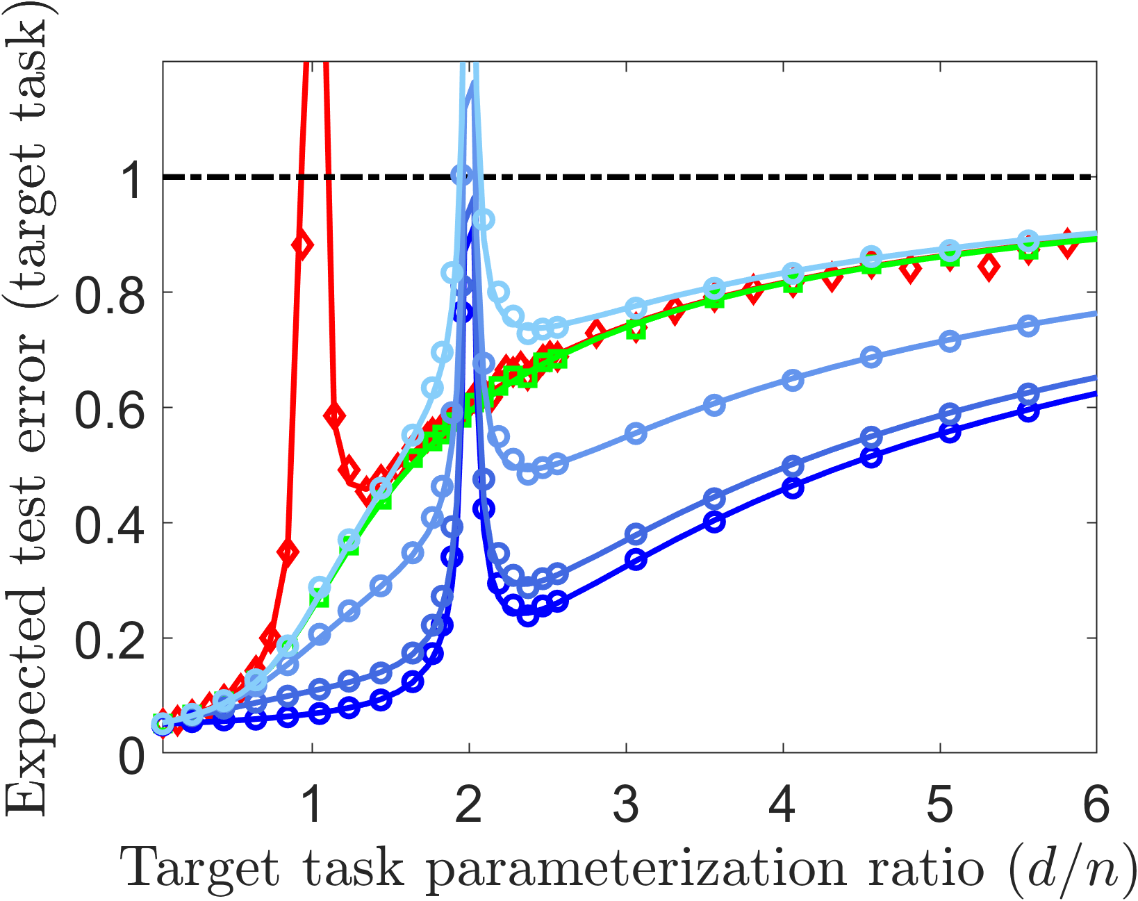
(a) Well specified

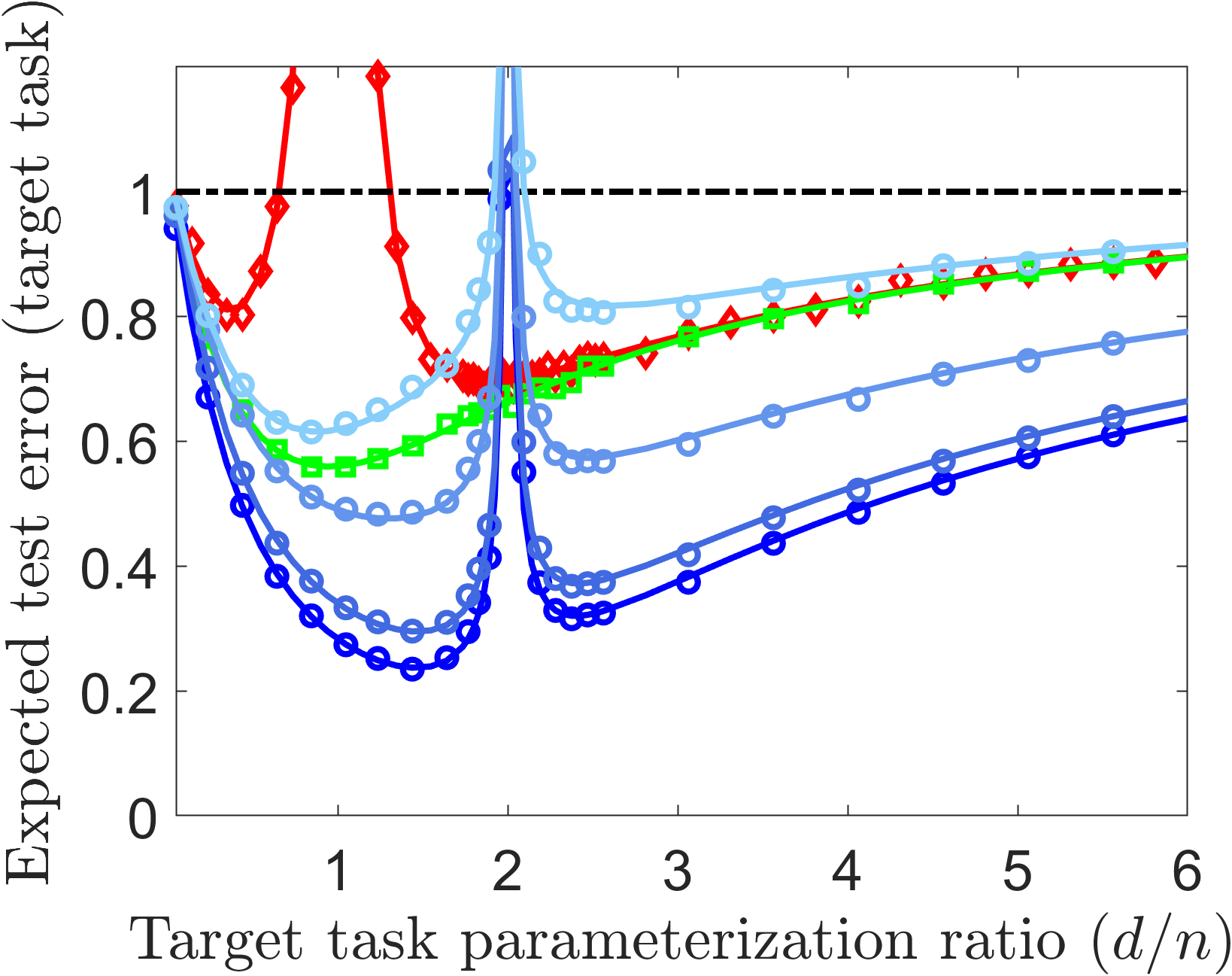
(b) Misspecified

(c)

Figure 1: The test error of the target task under isotropic Gaussian assumption on $\boldsymbol{\beta}$ and isotropic target features. Here $\widetilde{\mathbf{H}}=\mathbf{H}=\mathbf{\Psi}^{T}$ where $\mathbf{\Psi}$ is the orthonormal DCT matrix. Analytical results are presented in solid lines: red curves correspond to minimum $\ell_{2}$-norm (ML2N) solutions of the target task, green curves correspond to optimally tuned ridge regression, blue curves correspond to optimally tuned transfer learning (TL) in its intuitive form from Section 3. The corresponding empirical results (errors averaged over 150 experiments) are denoted by markers in the relevant colors. The number of data samples for the target task is $n=64$ and for the source task is $\widetilde{n}=128$. The misspecified models in (b) correspond to Assumptions 4-5 and polynomial reduction with $a=2.5$, $q=500$, $\rho=2$.

Theorem 4.2.

Consider Assumptions 1-2 and for $\widetilde{\mathbf{H}}=\mathbf{H}=\mathbf{\Psi}^{T}$ where $\mathbf{\Psi}$ is a $d\times d$ orthonormal matrix. The optimal tuning of the transfer learning solution (i.e., ${\alpha_{\rm TL}}>0$) from (7) is achieved for $d\notin\{\widetilde{n}-1,\widetilde{n},\widetilde{n}+1\}$ by setting ${\alpha_{\rm TL}}$ to

(10) $$\alpha_{\rm TL}^{\rm opt}=\frac{\sigma_{\epsilon}^{2}}{nC_{\rm TL}}$$

and the corresponding minimal test error is

(11) $$\bar{\mathcal{E}}_{\rm TL}^{\rm opt}=\sigma_{\epsilon}^{2}\left({1+\mathbb{E}_{\mathbf{X}_{\mathbf{\Psi}}}\left[{{\operatorname{Tr}\left\{{\left({\mathbf{X}_{\mathbf{\Psi}}^{T}\mathbf{X}_{\mathbf{\Psi}}+n\alpha_{\rm TL}^{\rm opt}\mathbf{I}_{d}}\right)^{-1}}\right\}}}\right]}\right).$$

For $d\in\{\widetilde{n}-1,\widetilde{n},\widetilde{n}+1\}$, $\bar{\mathcal{E}}_{\rm TL}=\infty$ for any ${\alpha_{\rm TL}}>0$.

Theorem 4.2 is proved in Appendix C.2. Note that the discontinuity of $C_{\rm TL}$ around $d=\widetilde{n}$ in (9) is a consequence of the infinite test error of the source model at $d\in\{\widetilde{n}-1,\widetilde{n},\widetilde{n}+1\}$ (see the error formulation in (29)). Consequently, plugging infinite-valued $C_{\rm TL}$ in the target test error in (8) leads to infinite test error $\bar{\mathcal{E}}_{\rm TL}$ for $d\in\{\widetilde{n}-1,\widetilde{n},\widetilde{n}+1\}$.

To develop the optimal test error from (11) into a more explicit analytical form, we will make use of an asymptotic setting, which is described next.

Assumption 3 (Asymptotic setting).

The quantities $d,n,\widetilde{n}\rightarrow\infty$ such that the target task parameterization level ${\frac{d}{n}\rightarrow\gamma_{\rm tgt}\in(0,\infty)}$, and the source task parameterization level $\frac{d}{\widetilde{n}}\rightarrow\gamma_{\rm src}\in(0,\infty)$. The task relation model ${\boldsymbol{\theta}=\mathbf{H}\boldsymbol{\beta}+\boldsymbol{\eta}}$ includes an operator $\mathbf{H}$ that satisfies ${\frac{1}{d}\left\|{{\mathbf{H}}}\right\|_{F}^{2}\rightarrow\kappa_{\mathbf{H}}}$. Moreover, the operator $\widetilde{\mathbf{H}}$ satisfies ${\frac{1}{d}\left\|{{\widetilde{\mathbf{H}}}}\right\|_{F}^{2}\rightarrow\kappa_{\widetilde{\mathbf{H}}}}$.

Our current case of $\mathbf{H}$ being an orthonormal matrix, and $\widetilde{\mathbf{H}}=\mathbf{H}$, implies that $\kappa_{\mathbf{H}}=\kappa_{\widetilde{\mathbf{H}}}=1$.

Theorem 4.3.

Consider Assumptions 1-3, ${d\notin\{{\widetilde{n}-1},\widetilde{n},{\widetilde{n}+1}\}}$, and $\widetilde{\mathbf{H}}=\mathbf{H}=\mathbf{\Psi}^{T}$ where $\mathbf{\Psi}$ is a $d\times d$ orthonormal matrix. Then, the transfer learning form of (7) whose ${\alpha_{\rm TL}}>0$ is optimally tuned to minimize the expected test error ${\bar{\mathcal{E}}_{\rm TL}}$ (i.e., with expectation w.r.t. the isotropic prior on $\boldsymbol{\beta}$) almost surely satisfies

(12) $${\bar{\mathcal{E}}_{\rm TL}^{\rm opt}}\rightarrow\sigma_{\epsilon}^{2}\left({1+\gamma_{\rm tgt}\cdot m\left(-\alpha_{{\rm TL},\infty}^{\rm opt};\gamma_{\rm tgt}\right)}\right)$$

where

(13) $$\alpha_{{\rm TL},\infty}^{\rm opt}=\sigma_{\epsilon}^{2}\gamma_{\rm tgt}\times\begin{cases}\mathmakebox[16em][l]{\left({\sigma_{\eta}^{2}+\frac{\gamma_{\rm src}\cdot\sigma_{\xi}^{2}}{1-\gamma_{\rm src}}}\right)^{-1}}\text{for }\gamma_{\rm src}<1\\ \mathmakebox[16em][l]{\left({\frac{\gamma_{\rm src}-1}{\gamma_{\rm src}}b+\frac{1}{\gamma_{\rm src}}\left({\sigma_{\eta}^{2}+\frac{\gamma_{\rm src}\cdot\sigma_{\xi}^{2}}{\gamma_{\rm src}-1}}\right)}\right)^{-1}}\text{for }\gamma_{\rm src}>1\end{cases}$$

is the limiting value of the optimal ${\alpha_{\rm TL}}>0$, and

(14) $$m\left(-\alpha_{{\rm TL},\infty}^{\rm opt};\gamma_{\rm tgt}\right)=\frac{-\left({1-\gamma_{\rm tgt}+\alpha_{{\rm TL},\infty}^{\rm opt}}\right)+\sqrt{\left({1-\gamma_{\rm tgt}+\alpha_{{\rm TL},\infty}^{\rm opt}}\right)^{2}+4\gamma_{\rm tgt}\alpha_{{\rm TL},\infty}^{\rm opt}}}{2\gamma_{\rm tgt}\alpha_{{\rm TL},\infty}^{\rm opt}}$$

is the Stieltjes transform of the Marchenko-Pastur distribution, which is the limiting spectral distribution of the sample covariance associated with $n$ samples that are drawn from a Gaussian distribution $\mathcal{N}\left(\mathbf{0},\mathbf{I}_{d}\right)$.

The proof outline of the last theorem is provided in Appendix C.3. The blue curves in Fig. 1a show the analytical formula for the test error ${\bar{\mathcal{E}}_{\rm TL}^{\rm opt}}$ of the optimally tuned transfer learning under Assumptions 1-3 and $\widetilde{\mathbf{H}}=\mathbf{H}$, for instances of the task relation model where $\mathbf{H}$ is an orthonormal matrix. Specifically, Fig. 1a shows transfer learning results for several noise variances $\sigma_{\eta}^{2}$.

Let us compare the test errors of the examined transfer learning approach with the corresponding errors of the minimum $\ell_{2}$-norm solution (recall the definition of $\widehat{\boldsymbol{\beta}}_{\rm ML2N}$ before (6)) that appear in red curves in Fig. 1a (see error formulation in Appendix C.4). One can observe that if the source and target tasks are sufficiently related (in terms of a sufficiently low task relation noise level $\sigma_{\eta}$), then the intuitive transfer learning approach indeed succeeds to resolve the peak that is induced by the ML2N solution and also to lower the test errors for the majority of parameterization levels. The only exception is that the examined transfer learning solution induces another peak in the generalization errors of the target task, and the location of this peak is determined by the point where the source task shifts from under to over parameterization. This is a side effect of transferring parameters from the source task, which by itself is a ML2N solution and therefore suffers from a peak of double descent in its own test error curves (see, e.g., (29)).

The test error peak in the examined transfer learning is an example for negative transfer, namely, a case where the target model learning can degrade due to using the source model. Specifically, in this work, we can identify a case as negative transfer if the test error for a transfer learning setting is higher than for the minimum $\ell_{2}$-norm solution and for the optimally tuned ridge regression (the latter will be characterized in Corollary 4.4). Other mathematical analyses of negative transfer, in other transfer learning methods, are provided in [7, 17].

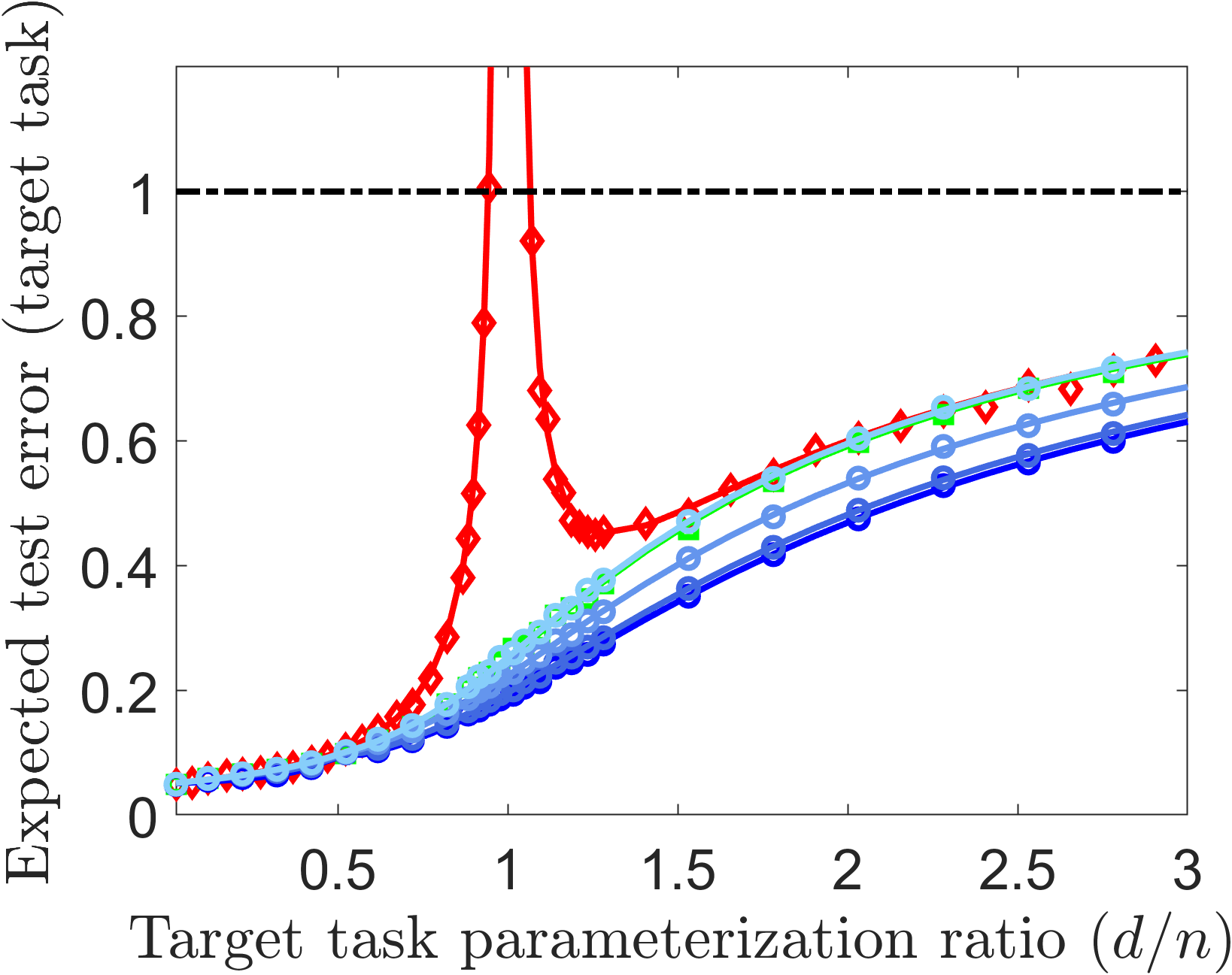
(a) Well specified

(b) Misspecified

(c)

Figure 2: The effect of less source training samples than target training samples, i.e., $n>\widetilde{n}$. Number of data samples for the target task is $n=128$ and for the source task is $\widetilde{n}=64$. The test error of the target task under isotropic Gaussian assumption on $\boldsymbol{\beta}$ and isotropic target features. Both subfigures refer to well specified settings with $\widetilde{\mathbf{H}}=\mathbf{H}$. In (a), $\mathbf{H}=\mathbf{\Psi}^{T}$ where $\mathbf{\Psi}$ is the orthonormal DCT matrix. In (b), $\mathbf{H}$ is a $d\times d$ circulant matrix corresponding to the discrete version of the continuous-domain convolution kernel ${h_{\rm ker}(\tau)=\delta(\tau)+e^{-\frac{\lvert\tau-0.5\rvert}{w_{\rm ker}}}}$ with  ${w_{\rm ker}=2/75}$. The non-orthonormal $\mathbf{H}$ is defined in more detail in Section 6.1.

4.2 The Test Error Peak in the Intuitive Transfer Learning: A Closer Look

It is natural to expect that the transferred source parameters would induce a peak in the target test error around the interpolation threshold of the source task, where the source model itself performs very poorly. Yet, one might also think that the optimal tuning of ${\alpha_{\rm TL}}>0$ in the intuitive transfer learning formula (7) would not perform much worse than the minimum $\ell_{2}$-norm solution to least squares (recall that setting ${\alpha_{\rm TL}}=0$ in the initial optimization form in (5) degenerates the transfer learning into a least squares problem). We now turn to explain this behavior in more detail.

The formulation in (13) for the optimal transfer learning parameter shows that as the setting approaches the source task interpolation threshold (namely, $\gamma_{\rm src}\rightarrow 1$ from the left or the right side of the limit), the optimal tuning approaches to zero ($\alpha_{{\rm TL},\infty}^{\rm opt}\rightarrow 0^{+}$). In the underparameterized regime of the target task, the matrix $\mathbf{X}$ is full rank and the limit of the transfer learning (7) for $\alpha_{{\rm TL},\infty}^{\rm opt}\rightarrow 0^{+}$ is the ordinary least squares regression:

(15) $$\text{For }\gamma_{\rm tgt}<1:~{}~{}~{}\lim_{\alpha_{{\rm TL},\infty}^{\rm opt}\rightarrow 0^{+}}\widehat{\boldsymbol{\beta}}_{\rm TL}=\left({\mathbf{X}^{T}\mathbf{X}}\right)^{-1}\mathbf{X}^{T}\mathbf{y}.$$

However, in the overparameterized regime of the target task, the matrix $\mathbf{X}$ is rank deficient. Accordingly, $\mathbf{X}^{T}\mathbf{X}$ has a $(d-n)$-dimensional null space, whose orthogonal projection matrix is $\mathbf{P}_{N(\mathbf{X})}\triangleq\mathbf{I}_{d}-\mathbf{X}^{+}\mathbf{X}$. Then, the transfer learning (7) for $\alpha_{{\rm TL},\infty}^{\rm opt}\rightarrow 0^{+}$ can be written as

(16) $$\text{For }\gamma_{\rm tgt}>1:~{}\lim_{\alpha_{{\rm TL},\infty}^{\rm opt}\rightarrow 0^{+}}\widehat{\boldsymbol{\beta}}_{\rm TL} =\left({\mathbf{X}^{T}\mathbf{X}}\right)^{+}\mathbf{X}^{T}\mathbf{y}+\mathbf{P}_{N(\mathbf{X})}\left({\widetilde{\mathbf{H}}^{T}\widetilde{\mathbf{H}}}\right)^{+}\widetilde{\mathbf{H}}^{T}\widehat{\boldsymbol{\theta}}$$

$$=\widehat{\boldsymbol{\beta}}_{\rm ML2N}+\mathbf{P}_{N(\mathbf{X})}\widetilde{\mathbf{H}}^{+}\widehat{\boldsymbol{\theta}}.$$

Eq. (16) shows that if the source task interpolation threshold occurs in the overparameterized regime of the target task, the corresponding optimal tuning (${\alpha_{{\rm TL},\infty}^{\rm opt}\rightarrow 0^{+}}$) leads to transfer learning that can significantly deviate from the minimum $\ell_{2}$-norm solution in the null space of the target data. Moreover, due to the involvement of $\widehat{\boldsymbol{\theta}}$, this deviation can increase the transfer learning error and cause a peak in the target test error around the interpolation threshold of the source task (where $\widehat{\boldsymbol{\theta}}$ has a poor performance by itself).

Equations (15)-(16) show that transferring the significant test error peak from the source task is possible only in the overparameterized regime of the optimally tuned transfer learning. Accordingly, we show in Fig. 2 the error curves for a setting where the target task has more training samples than the source task, namely, $n>\widetilde{n}$. In this setting, the source interpolation threshold resides in the underparameterized regime of the target task (for example, in Fig. 2 the source interpolation threshold is at $d/n=0.5$ whereas the target interpolation threshold is at $d/n=1$). Indeed, Fig. 2 exemplifies that, for $n>\widetilde{n}$, the optimally tuned intuitive transfer learning does not have a significant error peak around the source interpolation threshold.

Transfer learning is often motivated by insufficient training data for the target task, which is accommodated by using a source model that was trained on a large dataset. Therefore, the case of $n<\widetilde{n}$ is of main interest, and we will focus on it in the rest of this paper.

4.3 Transfer Learning versus Ridge Regression

Let us compare the transfer learning of (5) with the standard ridge regression approach, which is independent of the source task and does not involve any transfer learning aspect. We start in a non-asymptotic setting; i.e., without Assumption 3. The standard ridge regression approach can be formulated as

(17) $$\widehat{\boldsymbol{\beta}}_{\rm ridge} =\operatorname*{arg\,min}_{\mathbf{b}\in\mathbb{R}^{d}}\left\|\mathbf{y}-\mathbf{X}\mathbf{b}\right\|_{2}^{2}+n\alpha_{\rm ridge}\left\|\mathbf{b}\right\|_{2}^{2}=\left({\mathbf{X}^{T}\mathbf{X}+n\alpha_{\rm ridge}\mathbf{I}_{d}}\right)^{-1}{\mathbf{X}^{T}\mathbf{y}}.$$

Here $\alpha_{\rm ridge}>0$ is a parameter whose optimal value, which minimizes the expected test error of the target task, is $\alpha_{\rm ridge}^{\rm opt}=\frac{d\sigma_{\epsilon}^{2}}{nb}$, and the respective test error is

(18) $$\bar{\mathcal{E}}_{\rm ridge}^{\rm opt}=\sigma_{\epsilon}^{2}\left({1+\mathbb{E}_{\mathbf{X}}\left[{{\operatorname{Tr}\left\{{\left({\mathbf{X}^{T}\mathbf{X}+n\alpha_{\rm ridge}^{\rm opt}\mathbf{I}_{d}}\right)^{-1}}\right\}}}\right]}\right).$$

Related results for optimally tuned ridge regression were provided, e.g., in [29, 13]. See Appendix D.1 for the proof outline in our notations.

Note that the test error formulations for the optimally tuned transfer learning for the case of $\widetilde{\mathbf{H}}=\mathbf{H}$ and an orthonormal $\mathbf{H}$ in (11) and for the optimally tuned ridge regression in (18) are the same except for the optimal regularization parameters $\alpha_{\rm TL}^{\rm opt}$ and $\alpha_{\rm ridge}^{\rm opt}$, respectively. Accordingly, the cases where transfer learning is better than ridge regression are characterized for non-asymptotic settings as follows (see proof in Appendix D.2).

Corollary 4.4.

Consider $\widetilde{\mathbf{H}}=\mathbf{H}=\mathbf{\Psi}^{T}$ where $\mathbf{\Psi}$ is a $d\times d$ orthonormal matrix. Then, the test error of optimally tuned transfer learning, $\bar{\mathcal{E}}_{\rm TL}^{\rm opt}$, is lower than the test error of optimally tuned standard ridge regression, $\bar{\mathcal{E}}_{\rm ridge}^{\rm opt}$, if $\alpha_{\rm TL}^{\rm opt}>\alpha_{\rm ridge}^{\rm opt}$, which is satisfied if ${\sigma_{\eta}^{2}+\frac{d\cdot\sigma_{\xi}^{2}}{|d-\widetilde{n}|-1}<b}$ for $d\notin\{{\widetilde{n}-1,\widetilde{n},\widetilde{n}+1}\}$, and never for ${d\in\{{\widetilde{n}-1,\widetilde{n},\widetilde{n}+1}\}}$.

The formula for the test error of the optimally tuned ridge regression in asymptotic settings (that is, under Assumptions 2-3, without our transfer learning and source task aspects) was already provided in [13, 18]. For completeness of presentation we provide this formulation in our notations in Appendix D.3. In Fig. 1a we provide the analytical and empirical evaluations of the test error of the optimally tuned ridge regression solution (see green curves and markers). The results exhibit that if the source and target tasks are sufficiently related (e.g., the blue curves that correspond to $\sigma_{\eta}^{2}=0,0.1,0.5$), then the optimally tuned transfer learning approach outperforms the optimally tuned ridge regression solution for all the parameterization levels besides those in the proximity of the threshold between the under and over parameterized regimes of the source model. Remarkably, whereas ridge regression indeed resolves the peak of the double descent of the target task, the examined transfer learning approach can reduce the test errors much further and for a wide range of parameterization levels.

Corollary 4.4 characterizes the cases where using a sufficiently related source task is more useful than using the true prior of the desired $\boldsymbol{\beta}$. Moreover, we consider $\boldsymbol{\beta}$ to originate from an isotropic Gaussian distribution, hence, the optimally tuned ridge regression solution is the minimum MSE estimate of the target task parameters; i.e., the solution that minimizes the test error of the target task when only the sample data $\mathbf{X},\mathbf{y}$ are given. This means that we demonstrated a case where even though optimally tuned ridge regression is the best approach for solving the independent target task, it is not necessarily the best approach when there is an option to utilize transferred parameters from a sufficiently-related source task (e.g., low $\sigma_{\eta}^{2}$) that was already solved in a sufficiently accurate manner w.r.t. the source task goal (i.e., low $\sigma_{\xi}^{2}$ and high $|d-\widetilde{n}|$).

5 Misspecified Models: An Example for Beneficial Overparameterization

Our discussion so far has focused on the learning of well-specified models, namely, where the number of parameters $d$ corresponds to the dimension of both the learned $\widehat{\boldsymbol{\beta}}$ and true $\boldsymbol{\beta}$ vectors. In learning well-specified models using isotropic features, the test errors in the overparameterized regime are usually higher than in the underparameterized regime (see the detailed discussion in [18] for ML2N and ridge regression). Indeed, we see this behavior in all the well-specified methods that we examine in Fig. 1a. Nevertheless, it is also shown in [18] that ML2N regression can become highly beneficial in the overparameterized regime when the learned model is misspecified; namely, when the number of learned parameters in $\widehat{\boldsymbol{\beta}}$ is lower than the number of parameters in the true $\boldsymbol{\beta}$, and that this gap decreases as the learned model becomes more parameterized.

In our transfer learning setting we interpret the misspecification aspect as follows.

Assumption 4 (Misspecification of the target task).

The data model in (2) is extended into

(19) $$y=\mathbf{x}^{T}\boldsymbol{\beta}+{\mathbf{x}_{\rm ms}}^{T}\boldsymbol{\beta}_{\rm ms}+\epsilon$$

where the additional features $\mathbf{x}_{\rm ms}\in\mathbb{R}^{q}$ and true parameters $\boldsymbol{\beta}_{\rm ms}\in\mathbb{R}^{q}$ are ignored in the learning process that only estimates the $d$-dimensional $\boldsymbol{\beta}$ using its corresponding features $\mathbf{x}$. Moreover, the task relation model in (3) is extended into

(20) $$\boldsymbol{\theta}=\mathbf{H}\boldsymbol{\beta}+{\mathbf{H}_{\rm ms}}\boldsymbol{\beta}_{\rm ms}+\boldsymbol{\eta}$$

where $\mathbf{H}_{\rm ms}\in\mathbb{R}^{d\times q}$ corresponds to the misspecified parameters $\boldsymbol{\beta}_{\rm ms}$. Also, $\boldsymbol{\beta}_{\rm ms}$ and $\mathbf{x}_{\rm ms}$ are independent of $\epsilon$ and $\boldsymbol{\eta}$.

Importantly, the transfer learning utilizes the operator $\mathbf{H}$ but not the additional operator $\mathbf{H}_{\rm ms}$ from (20), implying that the misspecified transfer learning uses only a part of the task relation. Specifically, although in this section we still assume a known $\mathbf{H}$ and set $\widetilde{\mathbf{H}}=\mathbf{H}$ in (7), the operator $\mathbf{H}_{\rm ms}$ is unknown and not used in the learning.

Assumption 5 (Independent misspecification with isotropic features).

Consider a random $\boldsymbol{\beta}_{\rm ms}$ which is zero-mean, isotropic, and independent of (the possibly anisotropic) $\boldsymbol{\beta}$. The misspecified features $\mathbf{x}_{\rm ms}\sim\mathcal{N}\left(\mathbf{0},\mathbf{I}_{q}\right)$ are independent of the other $d$ features in $\mathbf{x}$. Also, $\mathbf{H}_{\rm ms}\mathbf{H}_{\rm ms}^{T}=\rho\mathbf{I}_{d}$ for $\rho\geq 0$, which implies that $q\geq d$ and $\mathbf{H}_{\rm ms}$ has orthogonal rows.

We assume that $\mathbb{E}\left[{{\left\|{{\boldsymbol{\beta}}}\right\|_{2}^{2}+\left\|{{\boldsymbol{\beta}_{\rm ms}}}\right\|_{2}^{2}}}\right]=\omega_{\boldsymbol{\beta}_{\rm all}}$ for the same constant $\omega_{\boldsymbol{\beta}_{\rm all}}$ for all $d,q$. Then, similarly to [18], we assume that the relative misspecification energy reduces polynomially as the parameterization level increases: $\mathbb{E}\left[{{\left\|{{\boldsymbol{\beta}_{\rm ms}}}\right\|_{2}^{2}}}\right]/\omega_{\boldsymbol{\beta}_{\rm all}}=\left(1+\frac{d}{n}\right)^{-a}$ for $a>0$. In Appendix B we show that under Assumptions 4-5, the misspecification effect is equivalent to learning of a well-specified model where the noise levels of $\epsilon$ and $\boldsymbol{\eta}$ are effectively higher (but this effective increase reduces with $d$). Such misspecification signficantly changes the behavior of the test error as a function of the parameterization level. Specifically, overparameterized models (i.e., where $d/n>1$) can achieve the best generalization performance — for example, see the results for an orthonormal $\mathbf{H}$ in Fig. 1b, the results for a circulant (non-orthonormal) $\mathbf{H}$ in Fig. 4, and additional results for stronger misspecification in Fig. 9 in Appendix B.2.

6 Unknown $\mathbf{H}$: Analysis for $\mathbf{H}$ and $\mathbf{\Sigma}_{\mathbf{x}}$ of General Forms

Having provided a detailed analytical characterization for the case where $\mathbf{H}$ is a known orthonormal matrix, we now proceed to the more intricate case where the matrix $\mathbf{H}$ is unknown and has a general form.

In this section, we examine the intuitive transfer learning approach from (7) with $\widetilde{\mathbf{H}}$ that might differ from the unknown $\mathbf{H}$. Then, the main question is how to choose $\widetilde{\mathbf{H}}$. Surprisingly, we will show that even the simple choice of $\widetilde{\mathbf{H}}=\mathbf{I}_{d}$ can perform well and, in some cases, can also outperform the seemingly better option of $\widetilde{\mathbf{H}}=\mathbf{H}$.

6.1 Analysis of the Intuitive Transfer Learning Approach

Recall that in our transfer learning approach (5) we do not have the true $\boldsymbol{\theta}$ but its estimate $\widehat{\boldsymbol{\theta}}$, which is the ML2N solution to the source task. The benefits from utilizing $\widehat{\boldsymbol{\theta}}$ in our transfer learning process (5) are affected by the distribution of the transferred source parameters $\widehat{\boldsymbol{\theta}}$. The second-order statistics of the distribution of $\widehat{\boldsymbol{\theta}}$ given the true target parameters $\boldsymbol{\beta}$ are formulated as follows (the proof is provided in Appendix E.1).

Proposition 6.1.

The expected value of $\widehat{\boldsymbol{\theta}}$ given $\boldsymbol{\beta}$ is

(21) $$\mathbb{E}\left[{{\widehat{\boldsymbol{\theta}}\big{|}\boldsymbol{\beta}}}\right]=\begin{cases}\mathmakebox[6em][l]{\mathbf{H}\boldsymbol{\beta}}\text{for }d\leq\widetilde{n},\\ \mathmakebox[6em][l]{\frac{\widetilde{n}}{d}\mathbf{H}\boldsymbol{\beta}}\text{for }d>\widetilde{n}.\end{cases}$$

The covariance matrix of $\widehat{\boldsymbol{\theta}}$ given $\boldsymbol{\beta}$, namely, $\mathbf{C}_{\widehat{\boldsymbol{\theta}}|\boldsymbol{\beta}}\triangleq\mathbb{E}\left[{{\left(\widehat{\boldsymbol{\theta}}-\mathbb{E}\left[{{\widehat{\boldsymbol{\theta}}\big{|}\boldsymbol{\beta}}}\right]\right)\left(\widehat{\boldsymbol{\theta}}-\mathbb{E}\left[{{\widehat{\boldsymbol{\theta}}\big{|}\boldsymbol{\beta}}}\right]\right)^{T}\Big{|}\boldsymbol{\beta}}}\right]$, is

(22) $$\mathbf{C}_{\widehat{\boldsymbol{\theta}}|\boldsymbol{\beta}}=\left(\frac{\sigma_{\eta}^{2}}{d}+\frac{\sigma_{\xi}^{2}}{\widetilde{n}-d-1}\right)\mathbf{I}_{d}$$

for $d\leq\widetilde{n}-2$, and

(23)

for $d\geq\widetilde{n}+2$. For $d\in\{\widetilde{n}-1,\widetilde{n},\widetilde{n}+1\}$ the covariance matrix is infinite valued.

In (23), ${\{\mathbf{H}\boldsymbol{\beta}\}_{j}}$ is the $j^{\rm th}$ component of the vector $\mathbf{H}\boldsymbol{\beta}$. The notation ${\rm diag}\left(\cdot\right)$ refers to the $d\times d$ diagonal matrix whose main diagonal values are specified as the arguments of ${\rm diag}\left(\cdot\right)$.

Proposition 6.1 demonstrates two very different forms of the covariance of $\widehat{\boldsymbol{\theta}}$: For an underparameterized source task with $d\leq\widetilde{n}-2$, the covariance is isotropic with a simple diagonal form that does not reflect $\boldsymbol{\beta}$ nor $\mathbf{H}$. However, for an overparameterized source task with $d\geq\widetilde{n}+2$, the covariance can be anisotropic with a form that depends on $\boldsymbol{\beta}$ and $\mathbf{H}$. This is a consequence of the ML2N solution to the source task, which by itself has two different error forms in its under- and over-parameterized cases.

Next, we turn to formulate the asymptotic generalization error for any asymptotic parameterization level $\frac{d}{n}\rightarrow\gamma_{\rm tgt}\in(0,\infty)$. The proof is provided in Appendix E.3.

Theorem 6.2.

Consider Assumptions 1-2, and general forms of $\widetilde{\mathbf{H}}$, $\mathbf{H}$ and $\mathbf{\Sigma}_{\mathbf{x}}$. Then, the transfer learning form of (7) with a (not necessarily optimal) parameter ${\alpha_{\rm TL}}>0$ almost surely satisfies

(24) $${\bar{\mathcal{E}}_{\rm TL}^{\rm opt}}\rightarrow\sigma_{\epsilon}^{2}\left(1+\gamma_{\rm tgt}\cdot\operatorname{Tr}\left\{{\frac{1}{d}\mathbf{W}\left(c(\alpha_{\rm TL})\mathbf{W}+\alpha_{\rm TL}\mathbf{I}_{d}\right)^{-1}}\right\}\right.$$

$$\left.+\gamma_{\rm tgt}\cdot\operatorname{Tr}\left\{{\left({\frac{\alpha_{\rm TL}^{2}}{\gamma_{\rm tgt}\sigma_{\epsilon}^{2}}\mathbf{\Gamma}_{{\rm TL},\infty}-\frac{\alpha_{\rm TL}}{d}\mathbf{I}_{d}}\right)\left(c(\alpha_{\rm TL})\mathbf{W}+\alpha_{\rm TL}\mathbf{I}_{d}\right)^{-1}s\mathbf{W}\left(c(\alpha_{\rm TL})\mathbf{W}+\alpha_{\rm TL}\mathbf{I}_{d}\right)^{-1}}\right\}\right)$$

where $\mathbf{W}\triangleq\left({\widetilde{\mathbf{H}}^{-1}}\right)^{T}\mathbf{\Sigma}_{\mathbf{x}}\widetilde{\mathbf{H}}^{-1}$, $s\triangleq c^{\prime}(\alpha_{\rm TL})+1$,

(25) $$\mathbf{\Gamma}_{{\rm TL},\infty}\triangleq\begin{cases}\mathmakebox[24em][l]{\frac{1}{d}\left({\sigma_{\eta}^{2}+\frac{\gamma_{\rm src}\cdot\sigma_{\xi}^{2}}{1-\gamma_{\rm src}}}\right)\mathbf{I}_{d}+\frac{b}{d}\left({\mathbf{H}-\widetilde{\mathbf{H}}}\right)\left({\mathbf{H}-\widetilde{\mathbf{H}}}\right)^{T}}\text{for }d\leq\widetilde{n}-2,\\ \mathmakebox[24em][l]{\infty}\text{for }\widetilde{n}-1\leq d\leq\widetilde{n}+1,\\ \mathmakebox[24em][l]{\frac{b(\gamma_{\rm src}-1)}{d\gamma_{\rm src}^{2}}\left({\gamma_{\rm src}\widetilde{\mathbf{H}}\widetilde{\mathbf{H}}^{T}-\mathbf{H}\mathbf{H}^{T}+\kappa_{\mathbf{H}}\mathbf{I}_{d}-\frac{1}{d}{\rm diag}\left({\{\left[\mathbf{H}\mathbf{H}^{T}\right]_{jj}\}_{j=1,\dots,d}}\right)}\right)}\\ \mathmakebox[24em][l]{+\frac{b}{d\gamma_{\rm src}}\left({\mathbf{H}-\widetilde{\mathbf{H}}}\right)\left({\mathbf{H}-\widetilde{\mathbf{H}}}\right)^{T}+\frac{1}{d\gamma_{\rm src}}\left({\sigma_{\eta}^{2}+\frac{\gamma_{\rm src}\cdot\sigma_{\xi}^{2}}{\gamma_{\rm src}-1}}\right)\mathbf{I}_{d}}\text{for }d\geq\widetilde{n}+2,\end{cases}$$

$c(\alpha_{\rm TL})$ is obtained as the solution of $\frac{1}{c(\alpha_{\rm TL})}-1=\frac{\gamma_{\rm tgt}}{d}\operatorname{Tr}\left\{{\mathbf{W}\left({c(\alpha_{\rm TL})\mathbf{W}+\alpha_{\rm TL}\mathbf{I}_{d}}\right)^{-1}}\right\}$, and then

(26) $$c^{\prime}(\alpha_{\rm TL})=\frac{\frac{\gamma_{\rm tgt}}{d}\left\|{{\mathbf{W}\left({c(\alpha_{\rm TL})\mathbf{W}+\alpha_{\rm TL}\mathbf{I}_{d}}\right)^{-1}}}\right\|_{F}^{2}}{(c(\alpha_{\rm TL}))^{-2}-\frac{\gamma_{\rm tgt}}{d}\left\|{{\mathbf{W}\left({c(\alpha_{\rm TL})\mathbf{W}+\alpha_{\rm TL}\mathbf{I}_{d}}\right)^{-1}}}\right\|_{F}^{2}}$$

where $\left\|{{\cdot}}\right\|_{F}$ is the Frobenius norm.

In Figs. 3, 4 we provide test error evaluations for well-specified and misspecified settings where $\mathbf{H}$ is a circulant matrix that corresponds to circular convolution with the discrete version ($d$ uniformly spaced samples) of the kernel function ${h_{\rm ker}(\tau)=\delta(\tau)+e^{-\frac{\lvert\tau-0.5\rvert}{w_{\rm ker}}}}$ defined for ${\tau\in[0,1]}$. Here $\delta(\cdot)$ is the Dirac delta. Note that the discrete convolution kernel is centered to have its peak value at the computed coordinate. Also, the discrete kernel is normalized such that the circulant matrix $\mathbf{H}$ satisfies ${\frac{1}{d}\left\|{{\mathbf{H}}}\right\|_{F}^{2}=1}$ for any $d$. Figs. 3, 4 show results for different values of the width parameter $w_{\rm ker}$. For a larger $w_{\rm ker}$ the operator $\mathbf{H}$ averages a larger neighborhood of coordinates and therefore the source task is less related to the target task, accordingly, Figures 3c, 3d, 4c, 4d in general show reduced gains from transfer learning compared to Figures 3a, 3b, 4a, 4b, respectively.

The results in Fig. 5 refer to a setting where $\mathbf{H}$ is a convolution with ${h_{\rm ker}}$ but in the DCT domain; namely, $\mathbf{H}$ is a composition of the $d\times d$ DCT matrix followed by the $d\times d$ circulant matrix that corresponds to ${h_{\rm ker}}$.

Figures 3, 4, 5 exemplify interesting behaviors that will be discussed in the next sections.

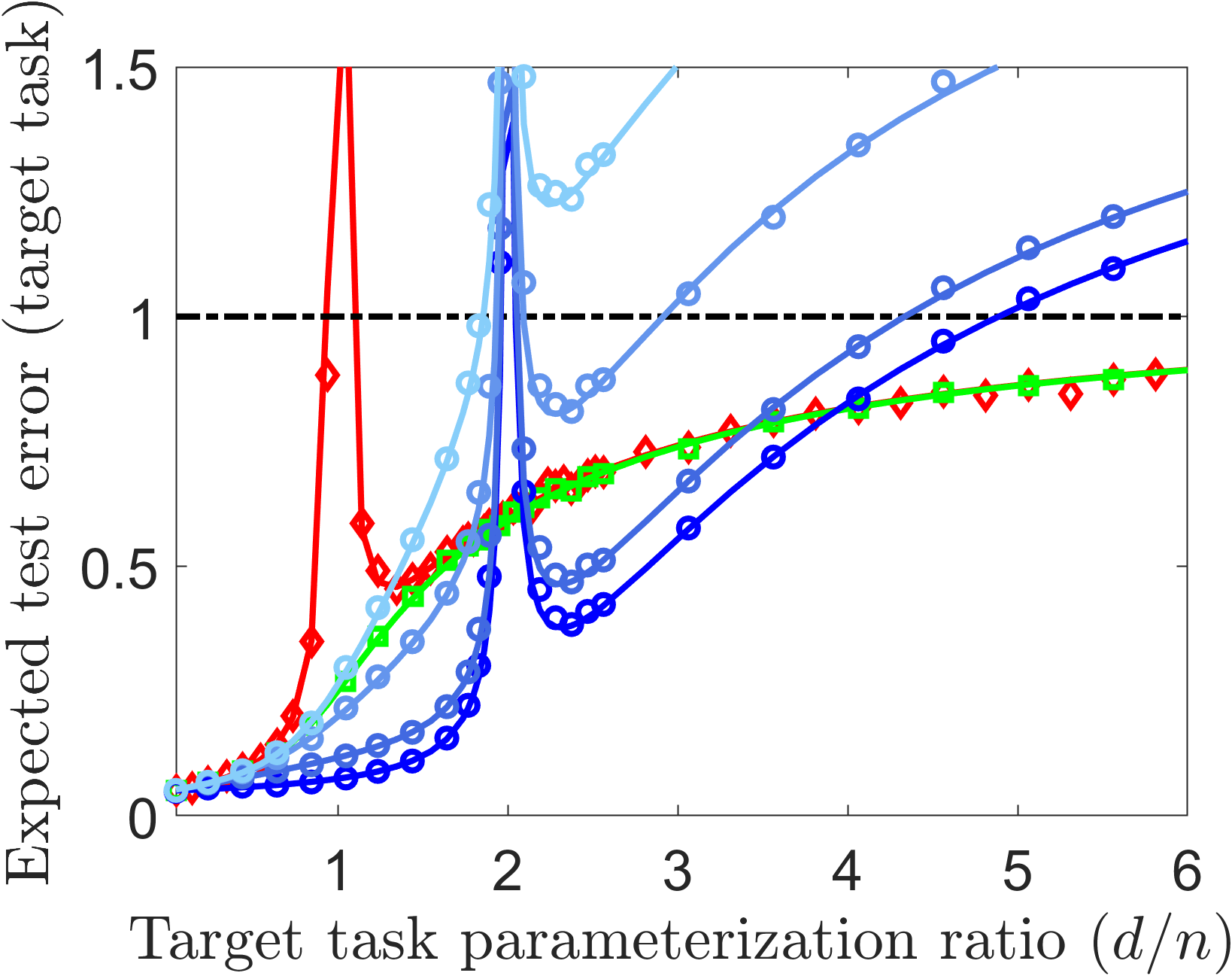
(a) Known $\mathbf{H}$ (${w_{\rm ker}=2/75}$): $\widetilde{\mathbf{H}}=\mathbf{H}$

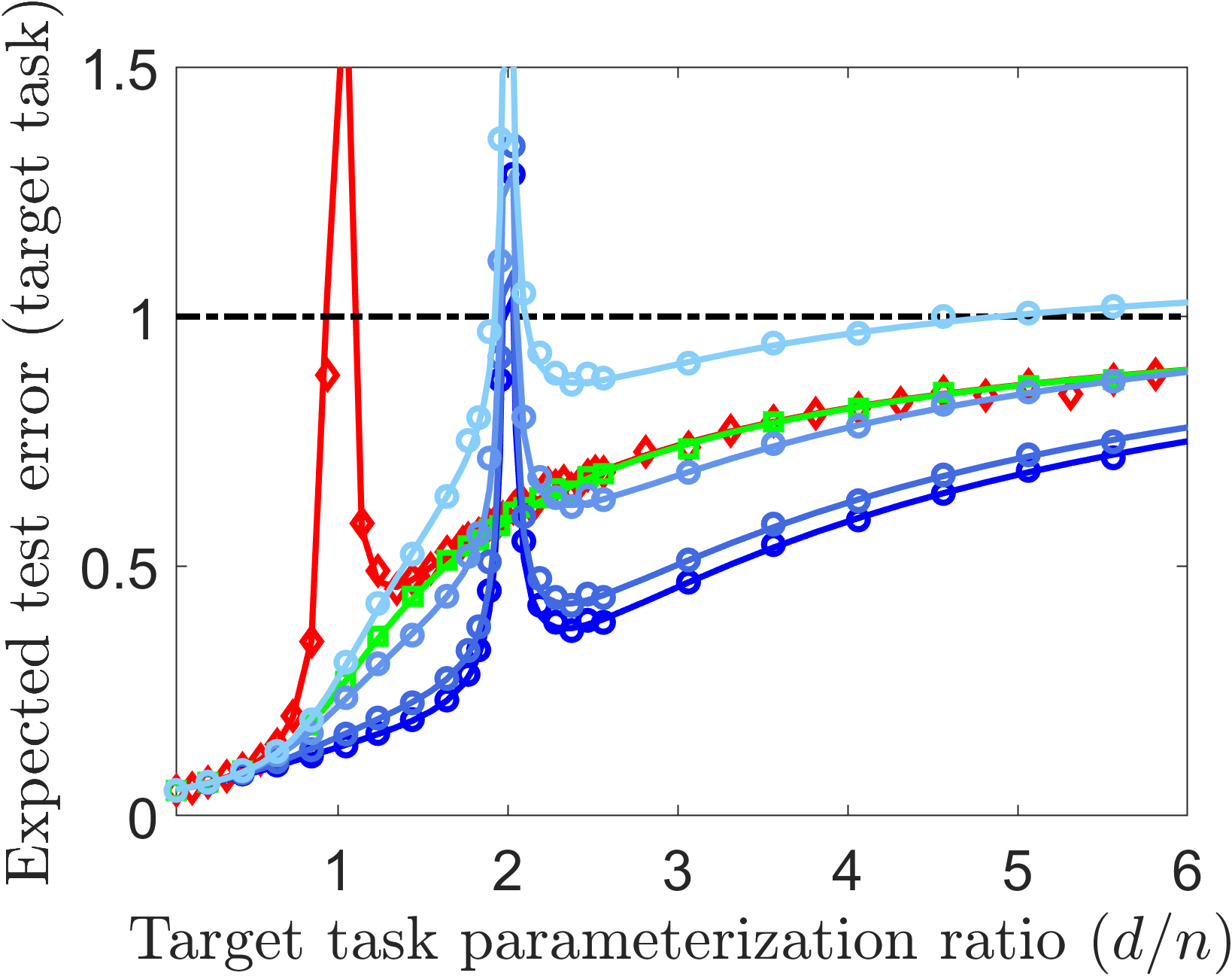
(b) Unknown $\mathbf{H}$ (${w_{\rm ker}=2/75}$): $\widetilde{\mathbf{H}}=\mathbf{I}_{d}$

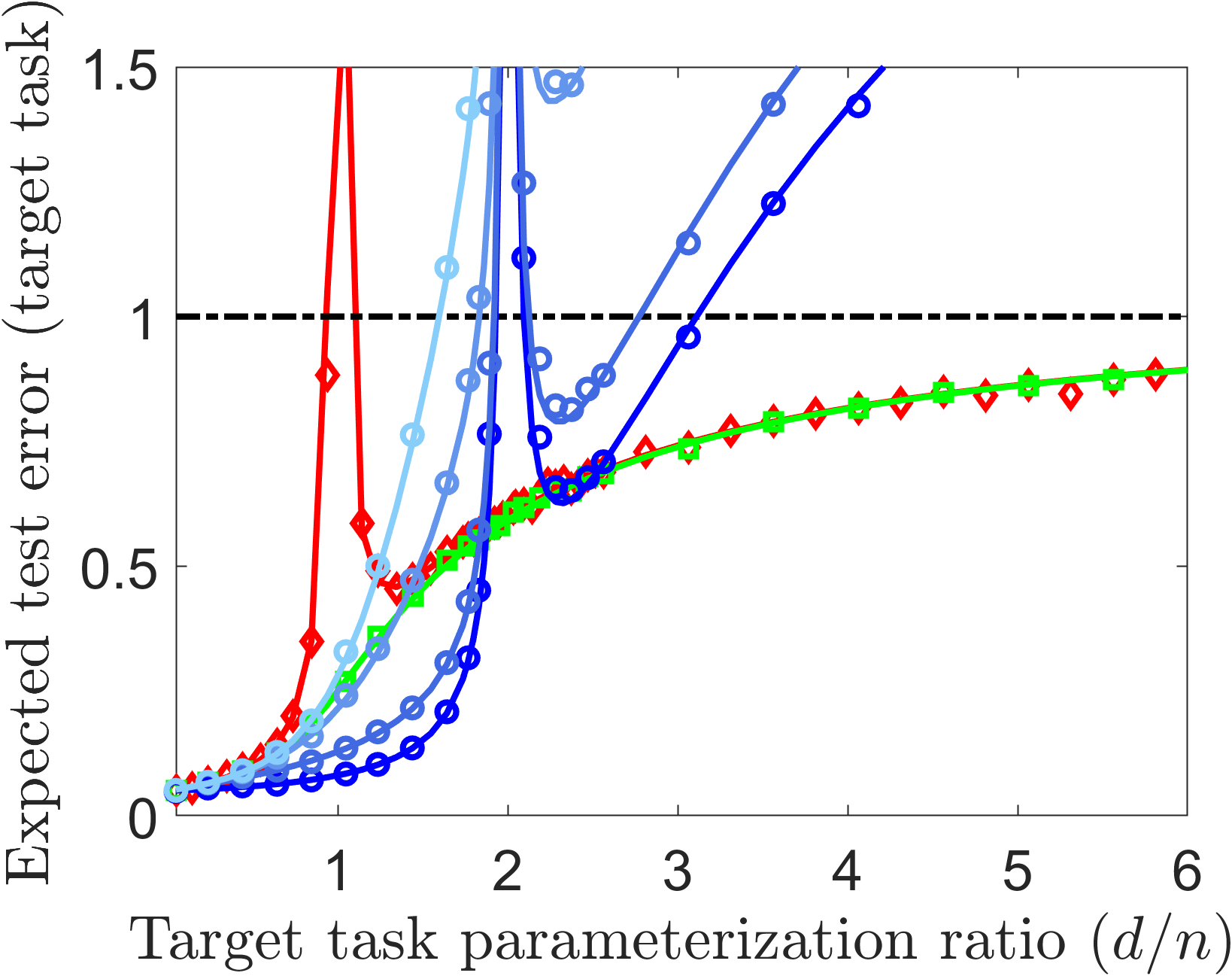
(c) Known $\mathbf{H}$ (${w_{\rm ker}=2/25}$): $\widetilde{\mathbf{H}}=\mathbf{H}$

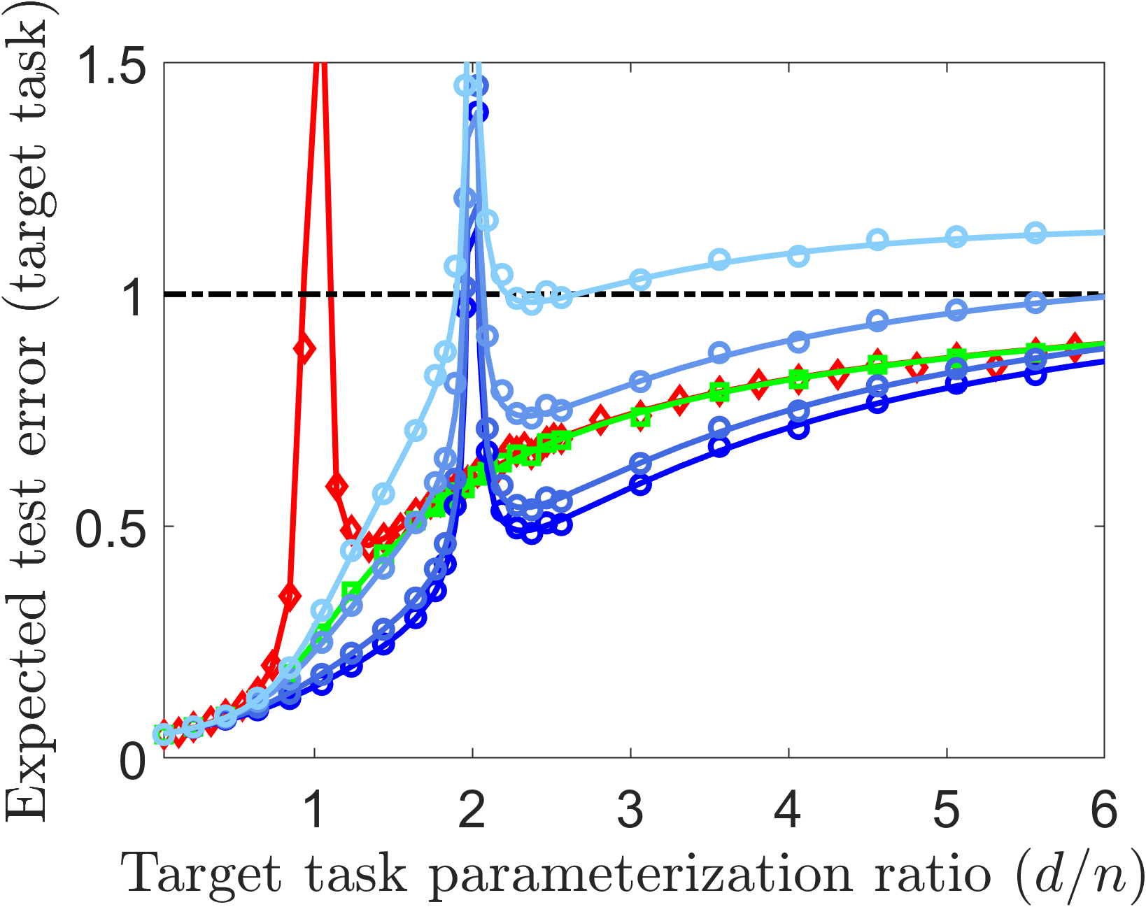
(d) Unknown $\mathbf{H}$ (${w_{\rm ker}=2/25}$): $\widetilde{\mathbf{H}}=\mathbf{I}_{d}$

(e)

Figure 3: The test error of the target task under isotropic Gaussian assumption on $\boldsymbol{\beta}$ and isotropic target features in a well specified setting. The matrix $\mathbf{H}$ is a $d\times d$ circulant matrix corresponding to the discrete version of the continuous-domain convolution kernel ${h_{\rm ker}(\tau)=\delta(\tau)+e^{-\frac{\lvert\tau-0.5\rvert}{w_{\rm ker}}}}$, here the kernel width is  ${w_{\rm ker}=2/75}$ in (a)-(b) and ${w_{\rm ker}=2/25}$ in (c)-(d). Curve colors and markers are as in Fig. 1. The number of data samples for the target task is $n=64$ and for the source task is $\widetilde{n}=128$.

(a) Known $\mathbf{H}$ (${w_{\rm ker}=2/75}$): $\widetilde{\mathbf{H}}=\mathbf{H}$

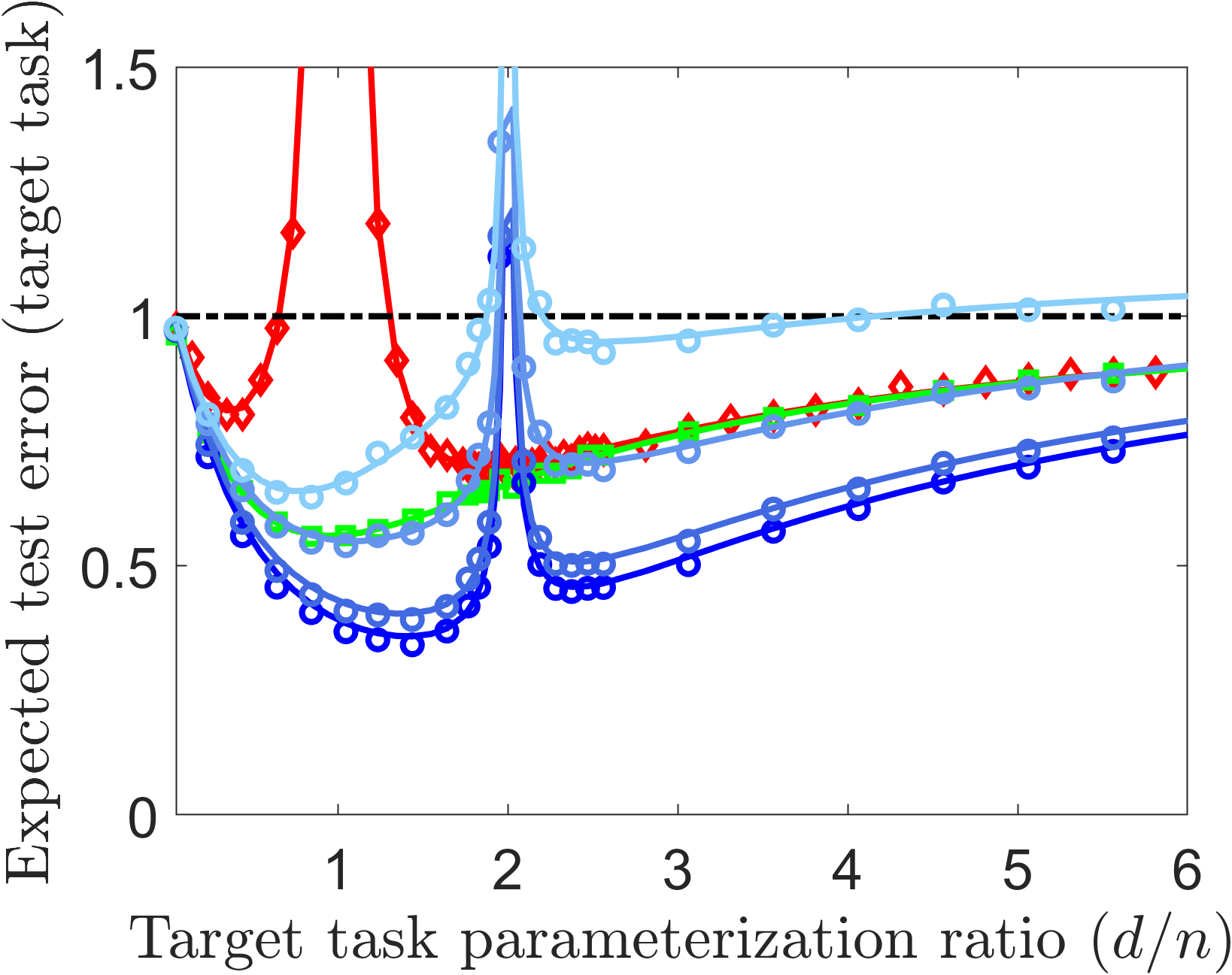
(b) Unknown $\mathbf{H}$ (${w_{\rm ker}=2/75}$): $\widetilde{\mathbf{H}}=\mathbf{I}_{d}$

(c) Known $\mathbf{H}$ (${w_{\rm ker}=2/25}$): $\widetilde{\mathbf{H}}=\mathbf{H}$

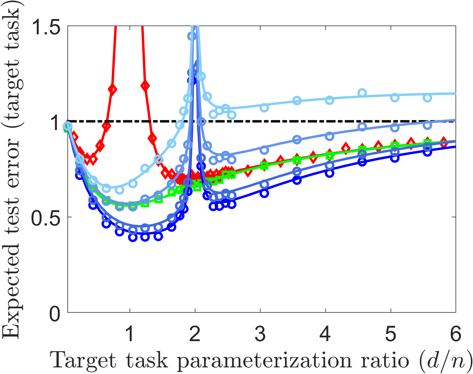
(d) Unknown $\mathbf{H}$ (${w_{\rm ker}=2/25}$): $\widetilde{\mathbf{H}}=\mathbf{I}_{d}$

(e)

Figure 4: The test error of the target task under isotropic Gaussian assumption on $\boldsymbol{\beta}$ and isotropic target features in a misspecified setting (according to Assumptions 4-5 and polynomial reduction with $a=2.5$, $q=500$, $\rho=2$). The matrix $\mathbf{H}$ is a $d\times d$ circulant matrix corresponding to the discrete version of the continuous-domain convolution kernel ${h_{\rm ker}(\tau)=\delta(\tau)+e^{-\frac{\lvert\tau-0.5\rvert}{w_{\rm ker}}}}$, here the kernel width is  ${w_{\rm ker}=2/75}$ in (a)-(b) and ${w_{\rm ker}=2/25}$ in (c)-(d). The number of data samples for the target task is $n=64$ and for the source task is $\widetilde{n}=128$.

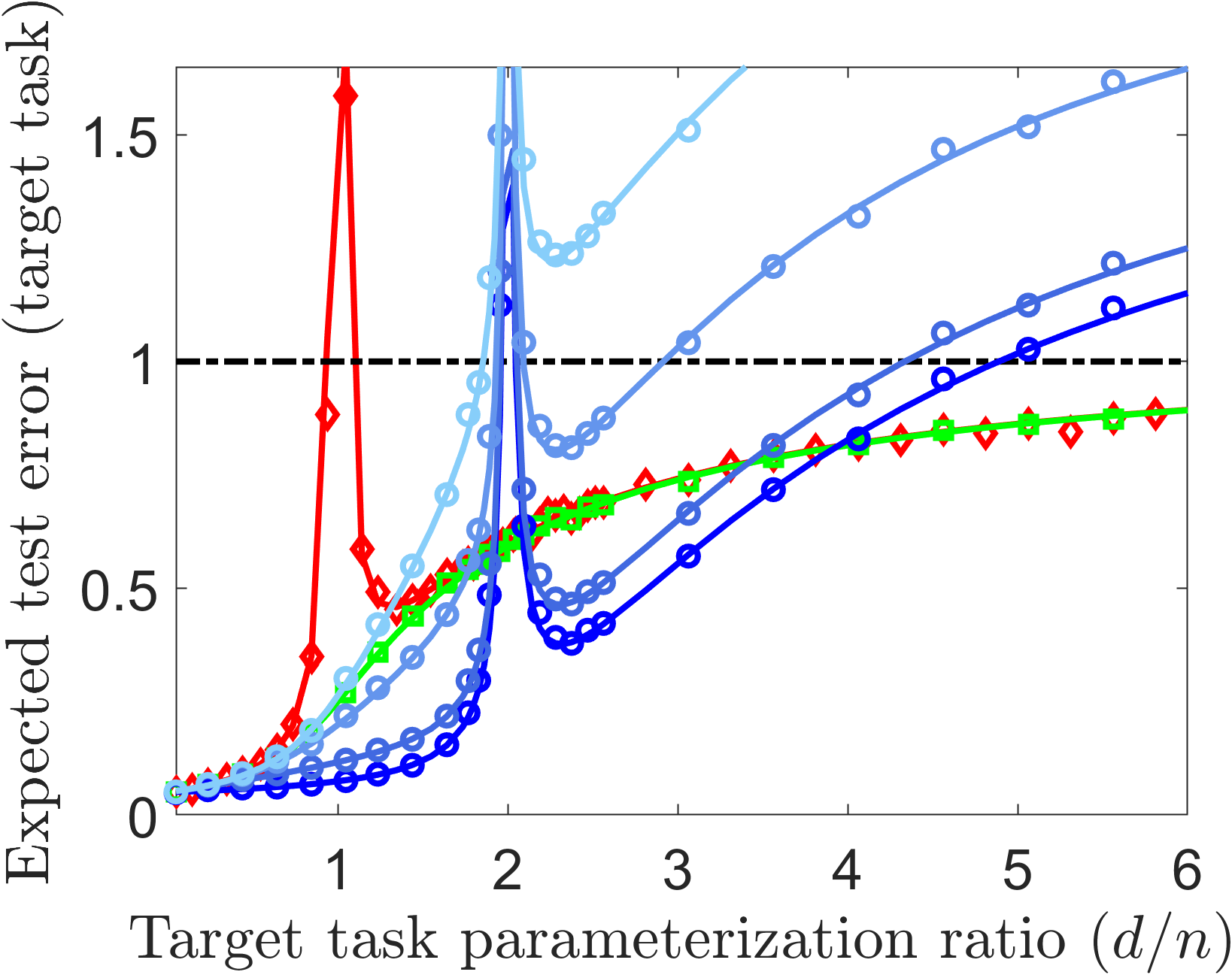
(a) Known $\mathbf{H}$ (conv. in DCT domain):
$\widetilde{\mathbf{H}}=\mathbf{H}$

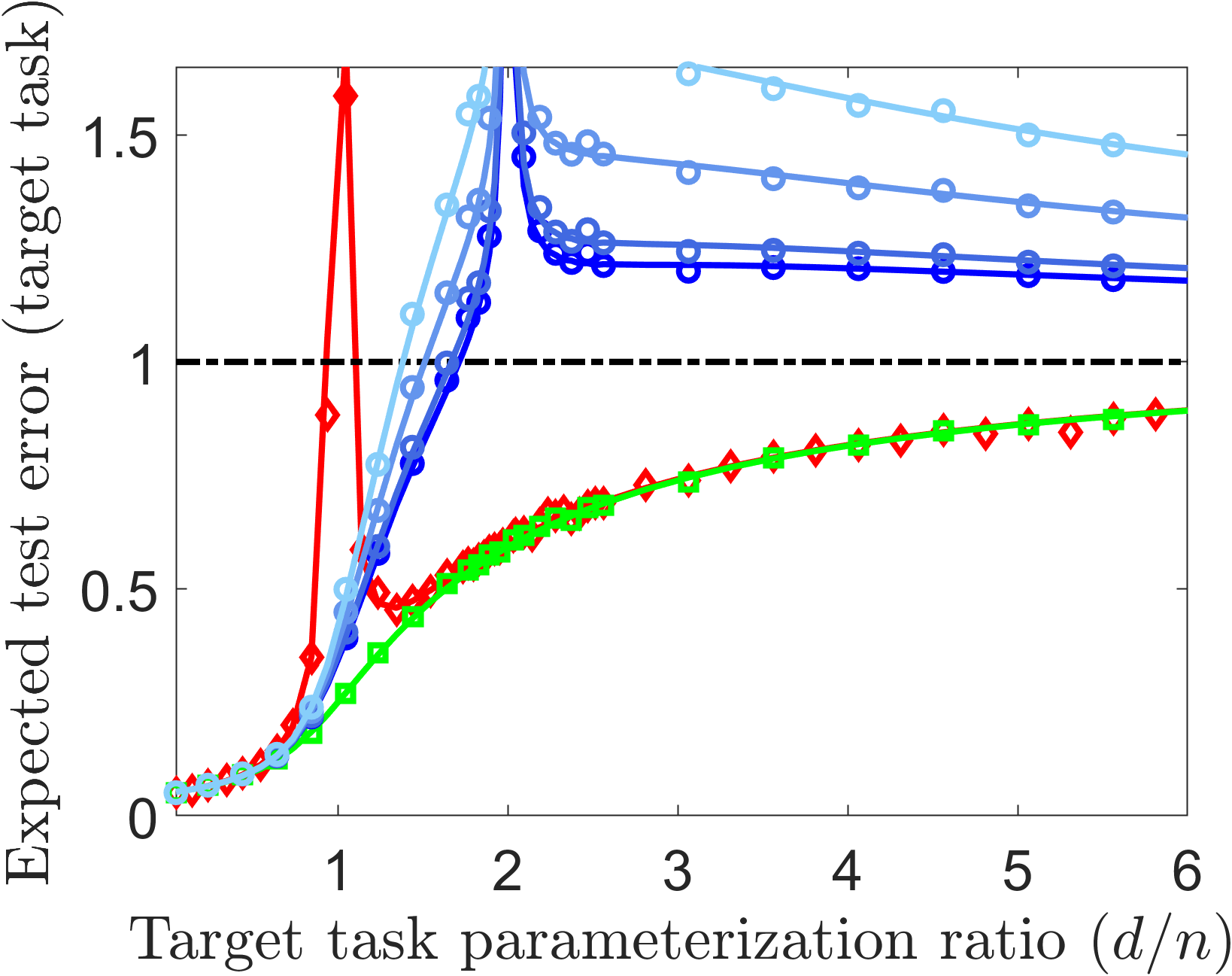
(b) Unknown $\mathbf{H}$ (conv. in DCT domain):
$\widetilde{\mathbf{H}}=\mathbf{I}_{d}$

(c)

Figure 5: The test error of the target task under isotropic Gaussian assumption on $\boldsymbol{\beta}$ and isotropic target features in a well specified setting. The matrix $\mathbf{H}$ is a $d\times d$ matrix corresponding to applying the discrete version of the continuous-domain convolution kernel ${h_{\rm ker}(\tau)=\delta(\tau)+e^{-\frac{\lvert\tau-0.5\rvert}{w_{\rm ker}}}}$ in the DCT domain, here the kernel width is  ${w_{\rm ker}=2/75}$. The number of data samples for the target task is $n=64$ and for the source task is $\widetilde{n}=128$.

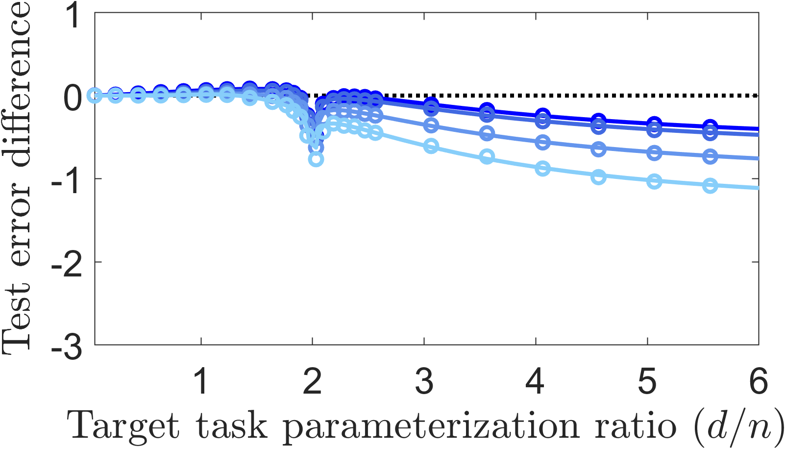
(a) ${w_{\rm ker}=2/75}$

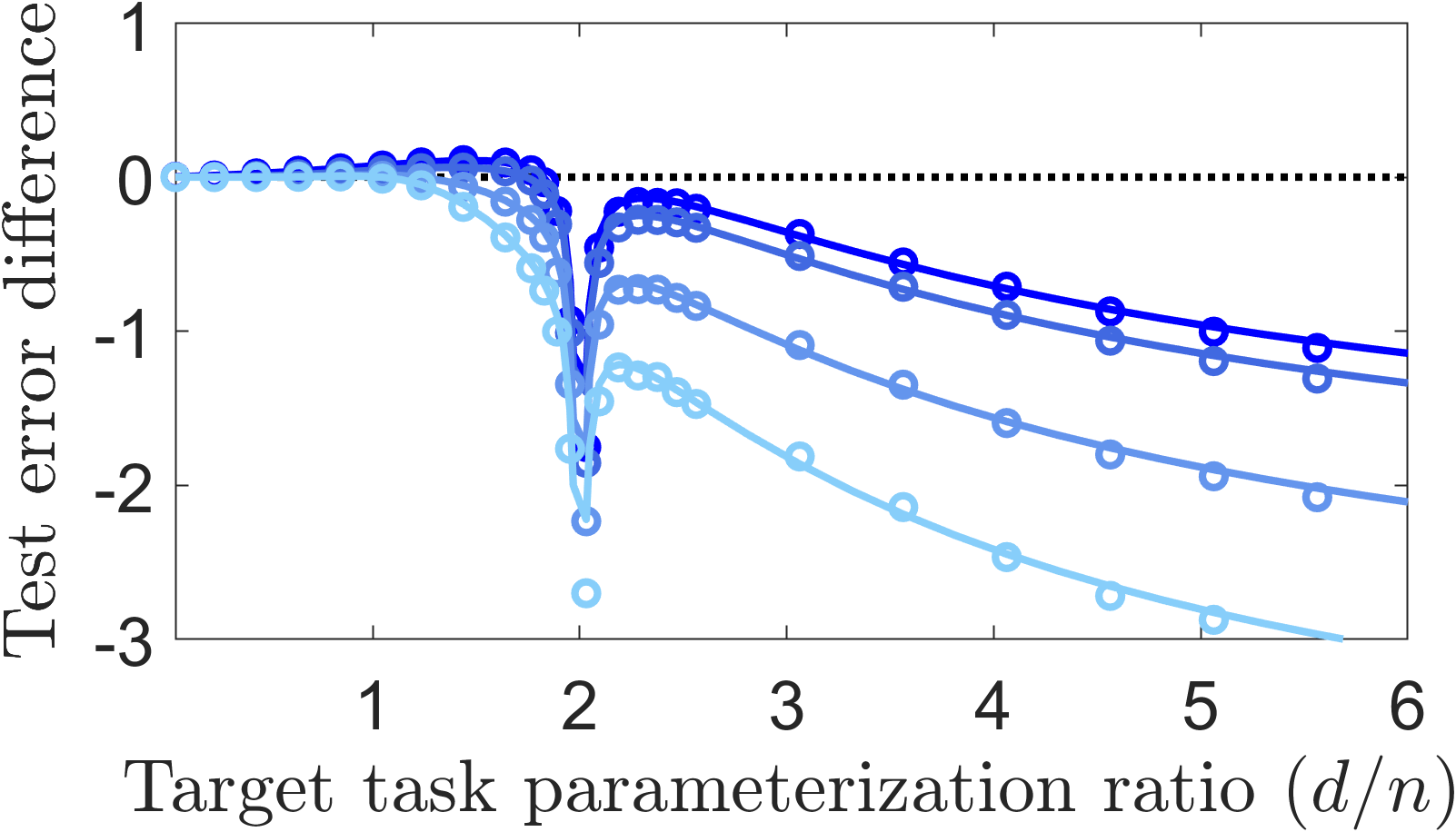
(b) ${w_{\rm ker}=2/25}$

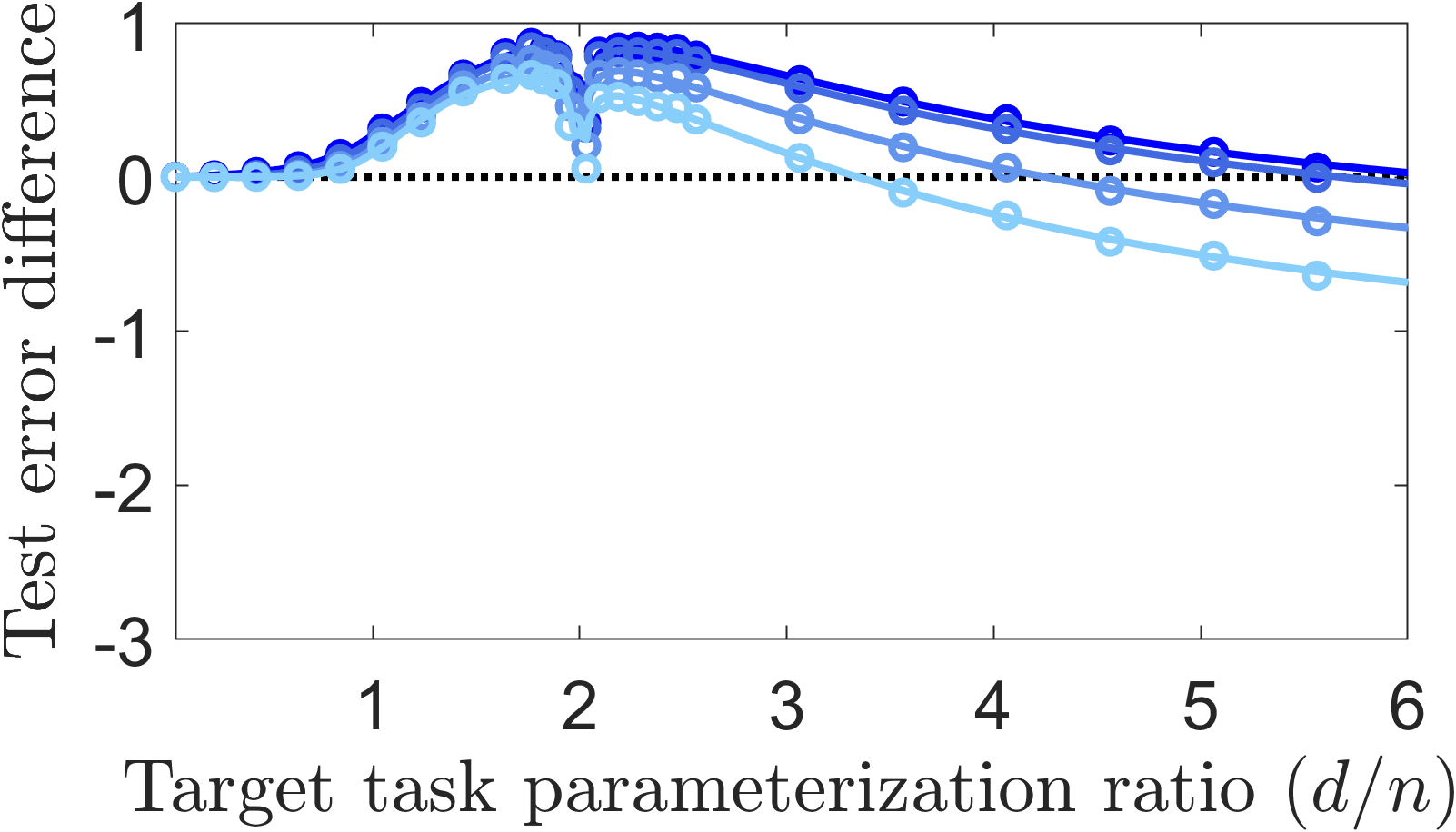
(c) ${w_{\rm ker}=2/75}$ in DCT domain

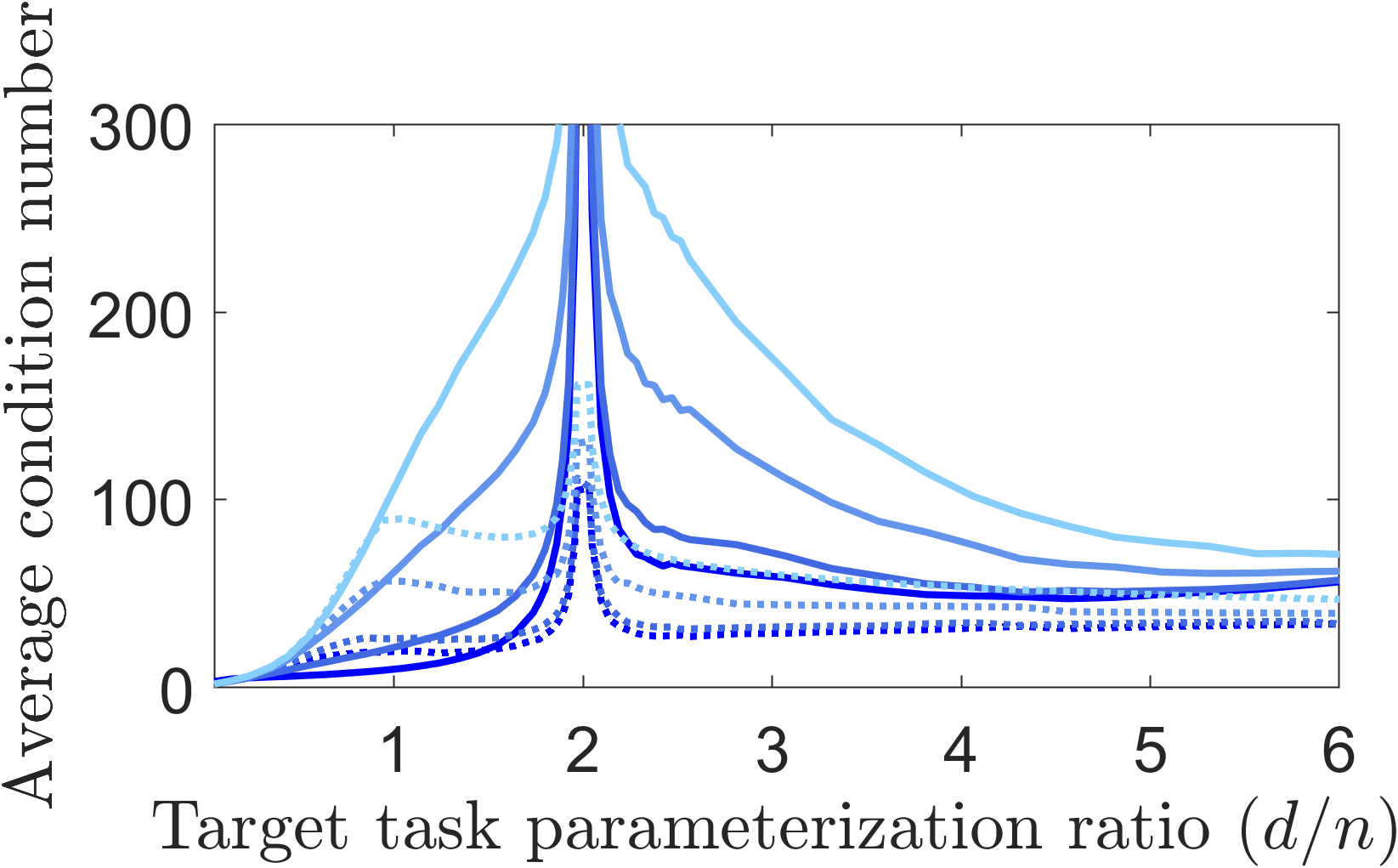
(d) ${w_{\rm ker}=2/75}$

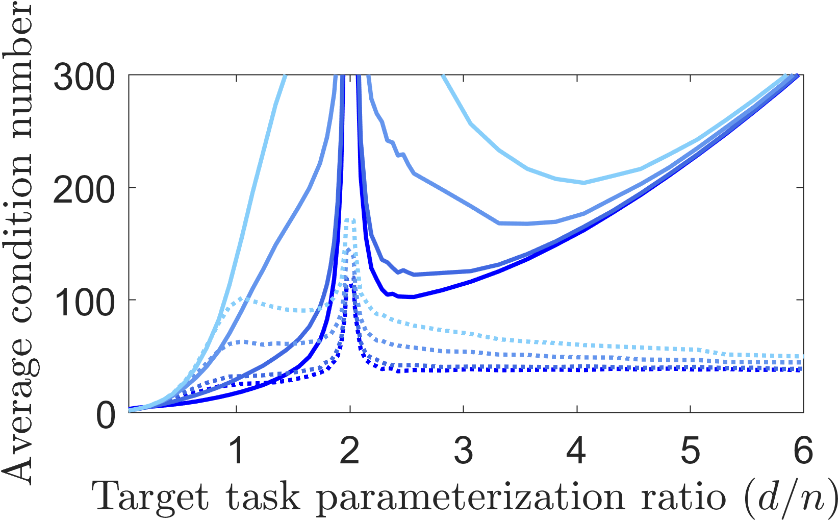
(e) ${w_{\rm ker}=2/25}$

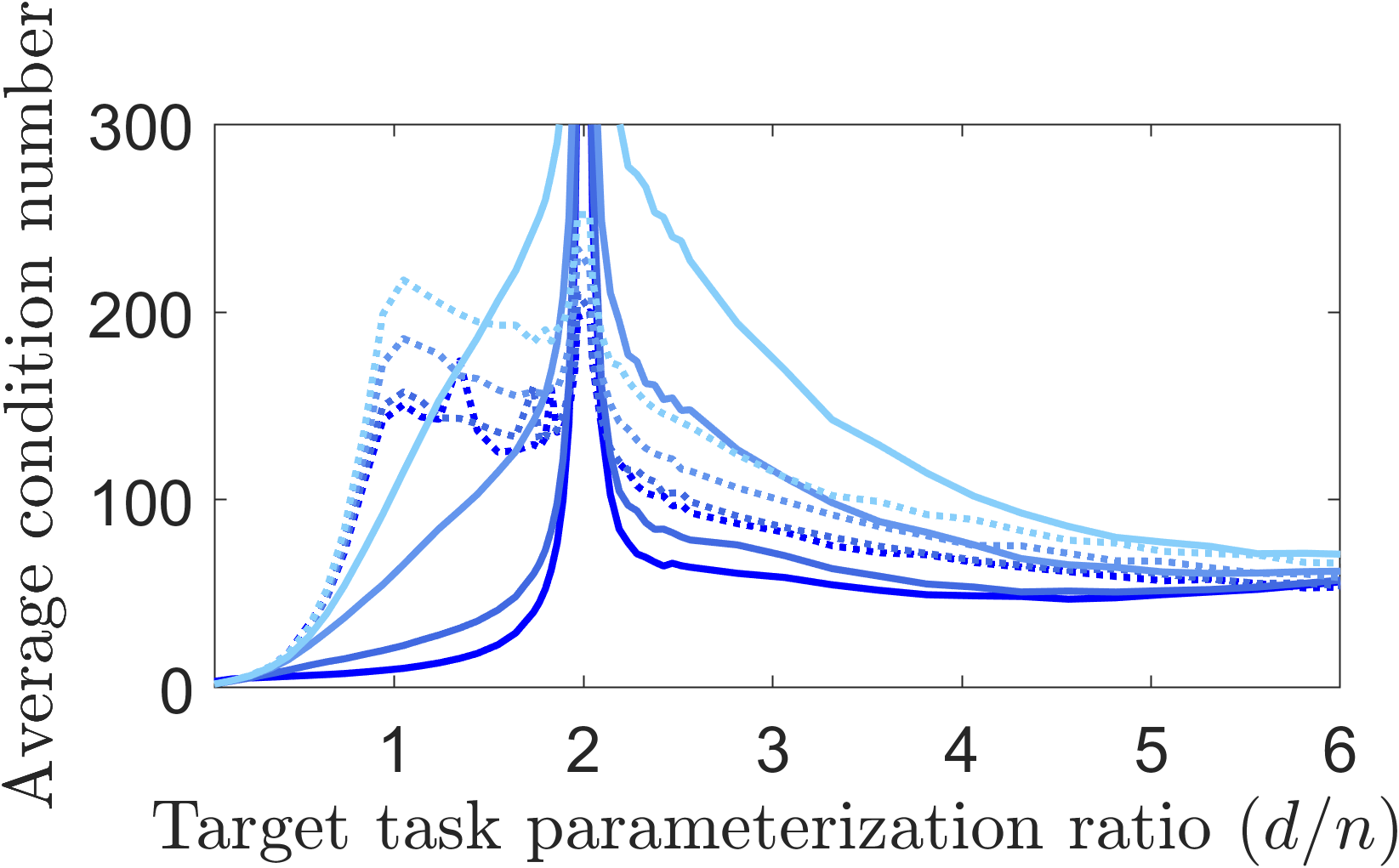
(f) ${w_{\rm ker}=2/75}$ in DCT domain

Figure 6: The test error difference between using $\widetilde{\mathbf{H}}=\mathbf{I}_{d}$ and $\widetilde{\mathbf{H}}=\mathbf{H}$ (subfigures (a)-(c), black dotted lines corresponds to zero difference). Each curve color corresponds to another noise level ($\sigma_{\eta}^{2}$) in the task relation, the colors refer to the same noise levels as in Fig. 3. The corresponding condition number of the matrix to invert (27) are presented in subfigures (d)-(f); solid lines refer to $\widetilde{\mathbf{H}}=\mathbf{H}$ and dotted lines refer to $\widetilde{\mathbf{H}}=\mathbf{I}_{d}$. Note that the peak of the condition number around the interpolation threshold of the source task are due to the optimal transfer learning parameter that is involved in the matrix in (27). These results are for isotropic Gaussian assumption on $\boldsymbol{\beta}$ and isotropic target features in a well specified setting. Each column of subfigures corresponds to another matrix $\mathbf{H}$ that is based on applying the discrete version of the continuous-domain convolution kernel ${h_{\rm ker}(\tau)=\delta(\tau)+e^{-\frac{\lvert\tau-0.5\rvert}{w_{\rm ker}}}}$ for ${w_{\rm ker}=2/75}$ (left column of subfigures), ${w_{\rm ker}=2/25}$ (middle column of subfigures), and ${w_{\rm ker}=2/75}$ in the DCT domain (right column of subfigures).

6.2 The Intuitive Transfer Learning can be Improved by Ignoring the True Task Relation

Let us examine the intuitive transfer learning method for $\widetilde{\mathbf{H}}=\mathbf{I}_{d}$ due to an unknown $\mathbf{H}$, and compare it to a setting where $\mathbf{H}$ is known and $\widetilde{\mathbf{H}}=\mathbf{H}$.

Remarkably, our results showcase that, in the overparameterized regime, the intuitive transfer learning with $\widetilde{\mathbf{H}}=\mathbf{I}_{d}$ can significantly outperform the intuitive transfer learning with a known $\mathbf{H}$ and $\widetilde{\mathbf{H}}=\mathbf{H}$. This behavior can be observed in several settings where the true $\mathbf{H}$ differs from $\mathbf{I}_{d}$; for example, compare the error curves of intuitive transfer learning (in the overparameterized regime) with a known $\mathbf{H}$ in Figs. 3a, 3c, 4a, 4c to their corresponding curves with an unknown $\mathbf{H}$ in Figs. 3b, 3d, 4b, 4d, respectively. Figures 6a-6c show the error differences of the corresponding error curves, such that a negative error difference implies that using $\widetilde{\mathbf{H}}=\mathbf{I}_{d}$ has a lower test error than using $\widetilde{\mathbf{H}}=\mathbf{H}$.

To explain the potential improvement despite ignoring the true $\mathbf{H}$, recall that the closed-form solution of the intuitive transfer learning in (7) includes an inversion of the matrix

(27) $$\mathbf{X}^{T}\mathbf{X}+n{\alpha_{\rm TL}}\widetilde{\mathbf{H}}^{T}\widetilde{\mathbf{H}}.$$

We consider a full rank $\widetilde{\mathbf{H}}$ (recall Assumption 1) and, therefore, the matrix in (27) is invertible. Yet, there is still a question of the ability of the solution to attenuate noise effectively.

The condition number of (27), namely, the ratio between the maximal and minimal eigenvalues of the matrix in (27), provides a useful way to characterize a linear system’s susceptibility to noise. Note that in the overparameterized regime, $\mathbf{X}$ is a $n\times d$ feature matrix where $d>n$ and, thus, the $d\times d$ matrix $\mathbf{X}^{T}\mathbf{X}$ is rank deficient with at least $d-n$ zero eigenvalues. Moreover, the singular values of the full-rank matrix $\widetilde{\mathbf{H}}$ are all non-zeros, but they can still be very small. A small singular value of $\widetilde{\mathbf{H}}$ yields a small eigenvalue of $\widetilde{\mathbf{H}}^{T}\widetilde{\mathbf{H}}$. Hence, for $\widetilde{\mathbf{H}}^{T}\widetilde{\mathbf{H}}$ with a considerable number of small eigenvalues, in highly overparameterized settings (where $\mathbf{X}^{T}\mathbf{X}$ is significantly rank deficient), the matrix in (27) is likely to have many small eigenvalues and a large condition number. To see why this is a problem, if we had $\mathbf{X}=\mathbf{0}$ (which is morally true on the null space of $\mathbf{X}$), then $\widehat{\boldsymbol{\beta}}_{\mathrm{TL}}=\widetilde{\mathbf{H}}^{+}\widehat{\boldsymbol{\theta}}$, meaning that any error in $\widehat{\boldsymbol{\theta}}$ is amplified by small singular values of $\widetilde{\mathbf{H}}$.

Setting $\widetilde{\mathbf{H}}=\mathbf{I}_{d}$ eliminates the error amplifying effects of small singuar values of $\widetilde{\mathbf{H}}$, which can be even more beneficial than using the true $\mathbf{H}$ in the intuitive transfer learning. Put differently, if setting $\widetilde{\mathbf{H}}=\mathbf{H}$ indeed amplifies error, there is a tradeoff between the errors induced by ignoring the true task relation and by the error amplification due to using the true task relation. For example, (24)-(25) show that using $\widetilde{\mathbf{H}}$ with a lower condition number can reduce error terms that involve $\widetilde{\mathbf{H}}^{-1}$ at the expense of some increase in the error terms that depend on the difference of $\widetilde{\mathbf{H}}$ from $\mathbf{H}$. In many cases, $\widetilde{\mathbf{H}}=\mathbf{I}_{d}$ addresses this tradeoff well and importantly shows that one does not have to use nor know $\mathbf{H}$!

Figures 3, 4, 5 and the error difference curves in Fig. 6 demonstrate when using $\widetilde{\mathbf{H}}=\mathbf{I}_{d}$ can outperform $\widetilde{\mathbf{H}}=\mathbf{H}$, and when it cannot. Whereas Figs. 6a, 6b clearly show the significant benefits of using $\widetilde{\mathbf{H}}=\mathbf{I}_{d}$ over using the true $\mathbf{H}$, Fig. 6c does not show such benefits except for the ultra high overparameterization levels. In Fig. 6c using $\widetilde{\mathbf{H}}=\mathbf{I}_{d}$ performs worse than $\widetilde{\mathbf{H}}=\mathbf{H}$ because the gap between the condition numbers of the two cases is moderate (Fig. 6f) and $\mathbf{H}$ is too far from $\mathbf{I}_{d}$ (due to the transformation to the DCT domain before the convolution). In contrast, the significant benefits of using $\widetilde{\mathbf{H}}=\mathbf{I}_{d}$ in Fig. 6b are reflected also by its ability to resolve the vast increase in the condition number of (27) for $\widetilde{\mathbf{H}}=\mathbf{H}$ in the highly overparameterized regime. Also, Figs. 6a, 6b show greater gains from using $\widetilde{\mathbf{H}}=\mathbf{I}_{d}$ when $\mathbf{H}$ is farther from $\mathbf{I}_{d}$ (i.e., note the greater gains for $\mathbf{H}$ with ${w_{\rm ker}=2/25}$ compared to ${w_{\rm ker}=2/75}$, although the latter is closer to $\mathbf{I}_{d}$).

More generally, we observed that using the true $\mathbf{H}$ in our intuitive transfer learning approach can be outperformed by other linear models that do not use the true $\mathbf{H}$. This raises the question of what is the optimal linear model for transfer learning with a known $\mathbf{H}$ — we will answer this question in the next section.

(a) Well specified, ${w_{\rm ker}=2/75}$

(b) Misspecified, ${w_{\rm ker}=2/75}$

(c) Well specified, ${w_{\rm ker}=2/25}$

(d) Misspecified, ${w_{\rm ker}=2/25}$

(e) Well specified, ${w_{\rm ker}=2/75}$ (in DCT domain)

(f)

Figure 7: The test error of the target task. Comparison of the intuitive transfer learning method to the LMMSE transfer learning method. Subfigures (a), (b), (c), (d), (e) extend Subfigures 3a, 4a, 3c, 4c, 5a, respectively, by adding the LMMSE error curves. Here, in each of the subfigures, one of the noise level $\sigma_{\eta}^{2}$ curves is absent for better visibility. All the results in this figure are for $\widetilde{\mathbf{H}}=\mathbf{H}$.

(a) Well specified, ${w_{\rm ker}=2/75}$

(b) Misspecified, ${w_{\rm ker}=2/75}$

(c) Well specified, ${w_{\rm ker}=2/25}$

(d) Misspecified, ${w_{\rm ker}=2/25}$

(e) Well specified, ${w_{\rm ker}=2/75}$ (in DCT domain)

(f)

Figure 8: The test error of the target task. Comparison of the intuitive transfer learning method to the LMMSE transfer learning method. Subfigures (a), (b), (c), (d), (e) extend Subfigures 3b, 4b, 3d, 4d, 5b, respectively, by adding the LMMSE error curves. Here, in each of the subfigures, one of the noise level $\sigma_{\eta}^{2}$ curves is absent for better visibility. All the results in this figure are for the intuitive TL with $\widetilde{\mathbf{H}}=\mathbf{I}_{d}$, but recall that the LMMSE TL always uses $\mathbf{H}$.

6.3 The Linear MMSE Solution to Transfer Learning

The intuitive transfer learning design (7) can perform excellently in a particular range of overparameterized settings; however, this performance can significantly degrade as the overparameterization further increases. This degradation is particularly evident for $\widetilde{\mathbf{H}}=\mathbf{H}$ where $\mathbf{H}$ is non-orthonormal, see Figs. 3a, 3c, 4a, 4c, 5a (in contrast, an orthonormal $\mathbf{H}$ has a condition number 1 and therefore the related matrix inversion does not lead to significant degradation, compared to ridge regression, in the overparameterized regime, see Fig. 1). Motivated by this degradation behavior, and since (7) is a linear estimator, we now turn to explore the optimal linear solution to our transfer learning problem.

Theorem 6.3.

Consider $\boldsymbol{\beta}$ as a zero mean random vector with a known covariance matrix $\mathbf{B}_{d}$. Then, the linear MMSE (LMMSE) estimate of $\boldsymbol{\beta}$ given the target dataset $\mathbf{X},\mathbf{y}$ and the precomputed source task solution $\widehat{\boldsymbol{\theta}}$:

(28) $$\widehat{\boldsymbol{\beta}}_{\rm LMMSE}=\begin{bmatrix}\mathbf{B}_{d}\mathbf{X}^{T}&\mathbb{E}\left[{{\boldsymbol{\beta}\widehat{\boldsymbol{\theta}}^{T}}}\right]\end{bmatrix}{\begin{bmatrix}\mathbf{X}\mathbf{B}_{d}\mathbf{X}^{T}+\sigma_{\epsilon}^{2}\mathbf{I}_{d}&\mathbf{X}\mathbb{E}\left[{{\boldsymbol{\beta}\widehat{\boldsymbol{\theta}}^{T}}}\right]\\ \mathbb{E}\left[{{\widehat{\boldsymbol{\theta}}\boldsymbol{\beta}^{T}}}\right]\mathbf{X}^{T}&\mathbb{E}\left[{{\widehat{\boldsymbol{\theta}}\widehat{\boldsymbol{\theta}}^{T}}}\right]\end{bmatrix}}^{-1}\begin{bmatrix}\mathbf{y}\\ \widehat{\boldsymbol{\theta}}\end{bmatrix}$$

where $\mathbb{E}\left[{{\boldsymbol{\beta}\widehat{\boldsymbol{\theta}}^{T}}}\right]=\left({\begin{cases}1&\text{for}~{}~{}d\leq\widetilde{n}\\ \frac{\widetilde{n}}{d}&\text{for}~{}~{}d>\widetilde{n}\end{cases}}\right)\times\mathbf{B}_{d}\mathbf{H}^{T}$ and

$$\mathbb{E}\left[{{\widehat{\boldsymbol{\theta}}\widehat{\boldsymbol{\theta}}^{T}}}\right]=\begin{cases}\mathmakebox[23em][l]{\mathbf{K}+\left({\frac{\sigma_{\eta}^{2}}{d}+\frac{\sigma_{\xi}^{2}}{\widetilde{n}-d-1}}\right)\mathbf{I}_{d}}\text{for }d\leq\widetilde{n}-2\\ \mathmakebox[23em][l]{\infty}\text{for }\widetilde{n}-1\leq d\leq\widetilde{n}+1\\ \mathmakebox[23em][l]{\frac{\widetilde{n}}{d}\left({\frac{\widetilde{n}+1}{d+1}\mathbf{K}+\frac{d-\widetilde{n}}{d^{2}-1}{\rm diag}\left({\{\operatorname{Tr}\left\{{\mathbf{K}}\right\}-k_{jj}\}_{j=1,\dots,d}}\right)+\left({\frac{\sigma_{\eta}^{2}}{d}+\frac{\sigma_{\xi}^{2}}{d-\widetilde{n}-1}}\right)\mathbf{I}_{d}}\right)}\\ \mathmakebox[23em][l]{~{}}\text{for }d\geq\widetilde{n}+2\end{cases}$$

where $\mathbf{K}\triangleq\mathbf{H}\mathbf{B}_{d}\mathbf{H}^{T}$ and $k_{jj}$ is its $(j,j)^{\rm th}$ component.

The proof of Theorem 6.3 is provided in Appendix E.4. According to the formulation in the theorem, the LMMSE naturally includes additional isotropic regularization (addition of a scaled $\mathbf{I}_{d}$) in the matrix inversion for the $\widehat{\boldsymbol{\theta}}$ component, which addresses the problem of the intuitive transfer learning with $\widetilde{\mathbf{H}}=\mathbf{H}$ when $\mathbf{H}$ is poorly conditioned. In this way, we can think of intuitive transfer learning with $\widetilde{\mathbf{H}}=\mathbf{I}_{d}$ as a coarse approximation to the LMMSE, except it does not use $\mathbf{H}$. Of course, the LMMSE will always perform better given complete knowledge.

The empirically-evaluated generalization errors of the LMMSE transfer learning solution are denoted by the purple markers in Figs. 7, 8. As expected, the errors of the LMMSE solution (for a known $\mathbf{H}$) lower bound the errors of the intuitive (linear) design to transfer learning from (7) with $\widetilde{\mathbf{H}}=\mathbf{H}$ (Fig. 7) or $\widetilde{\mathbf{H}}=\mathbf{I}_{d}$ (Fig. 8).

The results for general $\mathbf{H}$ and $\mathbf{\Sigma}_{\mathbf{x}}$ (Fig. 7) show that the LMMSE significantly improves the intuitive TL design at the highly overparameterized settings. Note that the LMMSE solution form in (28) is obtained by a linear processing of the “effective measurements” vector $\begin{bmatrix}\mathbf{y}\\ \widehat{\boldsymbol{\theta}}\end{bmatrix}$ that concatenates the source task solution to training data of the target task. Accordingly, the significant performance gains due to the LMMSE solution suggest that the common intuition to transfer learning implementation can sometimes be far from achieving the potential benefits of using the source task.

7 Conclusions

We have established a new perspective on transfer learning as a regularizer of overparameterized learning. We defined a transfer learning process between two linear regression tasks such that the target task is optimized with regularization on the distance of its learned parameters from parameters transferred from an already computed source task. We showed that the examined transfer learning method resolves the peak in the generalization errors of the minimum $\ell_{2}$-norm solution to the target task. We demonstrated that if the source task is sufficiently related to the target task and solved in sufficient accuracy, then optimally tuned transfer learning can significantly outperform optimally tuned ridge regression over a wide range of parameterization levels. Remarkably, we show that our transfer learning can perform well also without knowing the true task relation, and in various cases to outperform utilization of the true task relation. The generalization performance of our transfer learning can degrade at very high overparameterization levels. Hence, we show that this issue can be resolved by implementing the linear MMSE solution to transfer learning, whose form poses interesting questions on the common intuition to transfer learning designs. Future extensions may study other optimization formulations such as hybrid regularizers that merge the ideas of ridge regression and parameter transfer, and additional task relation models and their utilization in the transfer learning process.

Appendix A Additional Details for Section 2

A.1 The Test Error of the Source Task

The test input-response pair $\left({\mathbf{z}^{(\rm test)},v^{(\rm test)}}\right)$ is independently drawn from the $\left(\mathbf{z},v\right)$ distribution defined above. Given the input $\mathbf{z}^{(\rm test)}$, the source task goal is to estimate the response value $v^{(\rm test)}$ by the value ${\widehat{v}\triangleq\mathbf{z}^{({\rm test}),T}\widehat{\boldsymbol{\theta}}}$, where $\widehat{\boldsymbol{\theta}}$ is learned using $\widetilde{\mathcal{D}}$. We can assess the generalization performance of the source task using the test squared error ${\mathcal{E}_{\rm src}}\triangleq\mathbb{E}\left[{{\left(\widehat{v}-v^{(\rm test)}\right)^{2}}}\right]=\sigma_{\xi}^{2}+\mathbb{E}\left[{{\left\|{\widehat{\boldsymbol{\theta}}-\boldsymbol{\theta}}\right\|_{2}^{2}}}\right]$, where the expectation in the definition of ${\mathcal{E}_{\rm src}}$ is with respect to the test data $\left({\mathbf{z}^{(\rm test)},v^{(\rm test)}}\right)$ and the training data ${\widetilde{\mathcal{D}}}$. Note that $\widehat{\boldsymbol{\theta}}$ is a function of the training data. A lower value of ${\mathcal{E}_{\rm src}}$ reflects better generalization performance of the source task.

The source test error of the minimum $\ell_{2}$-norm solution (1) can be formulated in non-asymptotic settings as

(29) $${\mathcal{E}_{\rm src}}=\begin{cases}\mathmakebox[15em][l]{\left({1+\frac{d}{\widetilde{n}-d-1}}\right)\sigma_{\xi}^{2}}\text{for }d\leq\widetilde{n}-2,\\ \mathmakebox[15em][l]{\infty}\text{for }\widetilde{n}-1\leq d\leq\widetilde{n}+1,\\ \mathmakebox[15em][l]{\left({1+\frac{\widetilde{n}}{d-\widetilde{n}-1}}\right)\sigma_{\xi}^{2}+\left({1-\frac{\widetilde{n}}{d}}\right)\left\|{{\boldsymbol{\theta}}}\right\|_{2}^{2}}\text{for }d\geq\widetilde{n}+2,\end{cases}$$

which is a particular case of the results in [3, 7].

A.2 The Well-Specified Problem Setting at Different Resolutions

The target task solution is based on estimating the parameter vector $\boldsymbol{\beta}\in\mathbb{R}^{d}$. Let us assume that $\boldsymbol{\beta}$ is a random vector that follows a Gaussian prior distribution $\mathcal{N}(\mathbf{0},\mathbf{B}_{d})$ where $\mathbf{B}_{d}$ is the $d\times d$ covariance matrix of $\boldsymbol{\beta}$. For considering the same problem at different resolutions we will assume that ${\mathbb{E}\left[{{\left\|{{\boldsymbol{\beta}}}\right\|_{2}^{2}}}\right]=\operatorname{Tr}\left\{{\mathbf{B}_{d}}\right\}=\omega_{\boldsymbol{\beta}}}$ where $\omega_{\boldsymbol{\beta}}$ is the same positive real constant for all $d,n$. For example, the last assumption is satisfied by $\mathbf{B}_{d}=\frac{1}{d}\mathbf{I}_{d}$ that corresponds to an isotropic Gaussian prior distribution for $\boldsymbol{\beta}$ and a constant ${\omega_{\boldsymbol{\beta}}=1}$.

Next we characterize the way that the parameter vector of the source task and the relation model to the target task behave at the resolution induced by the dimension $d$. The relation between $\boldsymbol{\theta}$ and $\boldsymbol{\beta}$ as presented in (3) implies that $\boldsymbol{\theta}$ is a random vector that is defined by a noisy linear transformation of the random vector $\boldsymbol{\beta}$. Specifically, the distribution of $\boldsymbol{\theta}$ is multivariate Gaussian with zero mean and covariance matrix ${\mathbf{H}\mathbf{B}_{d}\mathbf{H}^{T}+\frac{\sigma_{\eta}^{2}}{d}\mathbf{I}_{d}}$. Similar to the above case of the target task parameters, for examining the same problem at different resolutions we assume that ${\mathbb{E}\left[{{\left\|{{\boldsymbol{\theta}}}\right\|_{2}^{2}}}\right]=\operatorname{Tr}\left\{{\mathbf{H}\mathbf{B}_{d}\mathbf{H}^{T}+\frac{\sigma_{\eta}^{2}}{d}\mathbf{I}_{d}}\right\}=\omega_{\boldsymbol{\theta}}}$ where ${\omega_{\boldsymbol{\theta}}}$ is the same positive real constant for all $d,n,\widetilde{n}$. In the case of ${\mathbf{B}_{d}=\frac{1}{d}\mathbf{I}_{d}}$, the last assumption is satisfied for ${\frac{1}{d}\left\|{{\mathbf{H}}}\right\|_{F}^{2}=\omega_{\mathbf{H}}}$ where $\omega_{\mathbf{H}}$ is the same positive real constant for all $d,n,\widetilde{n}$. Note the following examples that satisfy this rule:

1. Transformation to another basis: $\mathbf{H}=\mathbf{\Psi}_{d}^{T}$ where $\mathbf{\Psi}_{d}$ is a $d\times d$ real orthonormal matrix, i.e., $\mathbf{\Psi}_{d}^{T}\mathbf{\Psi}_{d}=\mathbf{I}_{d}$. Examples for such $\mathbf{\Psi}_{d}$ are the $d\times d$ forms of the identity matrix, discrete cosine transform (DCT) matrix, Hadamard matrix (the case of Hadamard is defined only for $d$ values that satisfy its recursive construction). In this setting, we study the generalization performance versus the dimension $d$ that is coupled with a $d\times d$ orthonormal matrix $\mathbf{\Psi}$ of the same type (e.g., DCT).

2. Circular convolution operation: In this case, $\mathbf{H}$ is a $d\times d$ circulant matrix that can be interpreted as a discrete version of the circular convolution kernel ${h_{\rm ker}:[0,1]\rightarrow\mathbb{R}}$, which is defined over the continuous interval ${[0,1]}$. The function ${h_{\rm ker}}$ is assumed to be smooth. Again, $\mathbf{H}$ should be properly scaled to ensure ${\frac{1}{d}\left\|{{\mathbf{H}}}\right\|_{F}^{2}=\omega_{\mathbf{H}}}$ where $\omega_{\mathbf{H}}$ is a constant independent of $d,n,\widetilde{n}$.

Appendix B Details and Proofs for Section 5

B.1 Independent Misspecification with Isotropic Features

Under Assumptions 4-5 we can develop the test error of the target task as follows. We learn a $d$-dimensional $\widehat{\boldsymbol{\beta}}$ and apply it on a test feature vector $\mathbf{x}^{(\rm test)}\in\mathbb{R}^{d}$ to obtain the response estimate $\widehat{y}=(\mathbf{x}^{(\rm test)})^{T}\widehat{\boldsymbol{\beta}}$. Meanwhile, the true test response has the form $y^{({\rm test})}=(\mathbf{x}^{({\rm test})})^{T}\boldsymbol{\beta}+(\mathbf{x}_{\rm ms}^{({\rm test})})^{T}\boldsymbol{\beta}_{\rm ms}+\epsilon^{({\rm test})}$. Then, the corresponding test error is

(30) $$\bar{\mathcal{E}}\triangleq\mathbb{E}\left[{{\left(\widehat{y}-y^{(\rm test)}\right)^{2}}}\right]=\sigma_{\epsilon}^{2}+\mathbb{E}\left[{{\left\|{\widehat{\boldsymbol{\beta}}-\boldsymbol{\beta}}\right\|_{\mathbf{\Sigma}_{\mathbf{x}}}^{2}}}\right]+\mathbb{E}\left[{{\left\|{\boldsymbol{\beta}_{\rm ms}}\right\|_{2}^{2}}}\right].$$

Now, consider a well specified model that corresponds to $y=\mathbf{x}^{T}\boldsymbol{\beta}+\widetilde{\epsilon}$, where ${\mathbf{x}\sim\mathcal{N}\left(\mathbf{0},\mathbf{\Sigma}_{\mathbf{x}}\right)}$ is $d$-dimensional and ${\widetilde{\epsilon}\sim\mathcal{N}\left(0,\widetilde{\sigma_{\epsilon}}^{2}\right)}$ with $\widetilde{\sigma_{\epsilon}}^{2}=\sigma_{\epsilon}^{2}+\mathbb{E}\left[{{\left\|{\boldsymbol{\beta}_{\rm ms}}\right\|_{2}^{2}}}\right]$. Then, the test error of this well-specified model is the same as the test error of the misspecified model from (30).

Next, under Assumptions 4-5 (specifically, recall that $\boldsymbol{\beta}$ and $\boldsymbol{\beta}_{\rm ms}$ are independent), the misspecified task relation model $\boldsymbol{\theta}=\mathbf{H}\boldsymbol{\beta}+{\mathbf{H}_{\rm ms}}\boldsymbol{\beta}_{\rm ms}+\boldsymbol{\eta}$ implies that $\boldsymbol{\theta}$ has zero mean and covariance

$$\mathbb{E}\left[{{\boldsymbol{\theta}\boldsymbol{\theta}^{T}}}\right] =\mathbf{H}\mathbb{E}\left[{{\boldsymbol{\beta}\boldsymbol{\beta}^{T}}}\right]\mathbf{H}^{T}+{\mathbf{H}_{\rm ms}}\mathbb{E}\left[{{\boldsymbol{\beta}_{\rm ms}\boldsymbol{\beta}_{\rm ms}^{T}}}\right]{\mathbf{H}_{\rm ms}^{T}}+\mathbb{E}\left[{{\boldsymbol{\eta}\boldsymbol{\eta}^{T}}}\right]$$

$$=\mathbf{H}\mathbf{B}_{d}\mathbf{H}^{T}+b_{\rm ms}{\mathbf{H}_{\rm ms}}{\mathbf{H}_{\rm ms}^{T}}+\sigma_{\eta}^{2}\mathbf{I}_{d}$$

$$=\mathbf{H}\mathbf{B}_{d}\mathbf{H}^{T}+b_{\rm ms}\rho\mathbf{I}_{d}+\sigma_{\eta}^{2}\mathbf{I}_{d}$$

(31) $$=\mathbf{H}\mathbf{B}_{d}\mathbf{H}^{T}+(b_{\rm ms}\rho+\sigma_{\eta}^{2})\mathbf{I}_{d}$$

where we denote $\mathbb{E}\left[{{\boldsymbol{\beta}_{\rm ms}\boldsymbol{\beta}_{\rm ms}^{T}}}\right]=b_{\rm ms}\mathbf{I}_{q}$ for some constant $b_{\rm ms}\geq 0$. Accordingly, we define $\widetilde{\boldsymbol{\eta}}\triangleq{\mathbf{H}_{\rm ms}}\boldsymbol{\beta}_{\rm ms}+\boldsymbol{\eta}$ and note that $\widetilde{\boldsymbol{\eta}}\sim\mathcal{N}(\mathbf{0},(b_{\rm ms}\rho+\sigma_{\eta}^{2})\mathbf{I}_{d})$ is independent of $\boldsymbol{\beta}$. Hence, the well-specified task relation $\boldsymbol{\theta}=\mathbf{H}\boldsymbol{\beta}+\widetilde{\boldsymbol{\eta}}$ is equivalent to the above misspecified model.

Recall that in Section 5 we assume that $\mathbb{E}\left[{{\left\|{{\boldsymbol{\beta}}}\right\|_{2}^{2}+\left\|{{\boldsymbol{\beta}_{\rm ms}}}\right\|_{2}^{2}}}\right]=\omega_{\boldsymbol{\beta}_{\rm all}}$ for the same constant $\omega_{\boldsymbol{\beta}_{\rm all}}$ for all $d,q$, and that $\mathbb{E}\left[{{\left\|{{\boldsymbol{\beta}_{\rm ms}}}\right\|_{2}^{2}}}\right]/\omega_{\boldsymbol{\beta}_{\rm all}}=\left(1+\frac{d}{n}\right)^{-a}$ for $a>0$. This implies that the variance of a misspecified parameter is $b_{\rm ms}=\frac{\omega_{\boldsymbol{\beta}_{\rm all}}}{q}\left(1+\frac{d}{n}\right)^{-a}$, which reflects the reduction in the misspecification level as the number of utilized features $d$ increases.

B.2 Additional Examples for Generalization Performance in Misspecified Settings

(a) $\widetilde{\mathbf{H}}=\mathbf{H}$

(b) $\widetilde{\mathbf{H}}=\mathbf{I}_{d}$

(c)

Figure 9: The test error of the target task under isotropic Gaussian assumption on $\boldsymbol{\beta}$ and isotropic target features. The matrix $\mathbf{H}$ is a $d\times d$ circulant matrix corresponding to the discrete version of the continuous-domain convolution kernel ${h_{\rm ker}(\tau)=\delta(\tau)+e^{-\frac{\lvert\tau-0.5\rvert}{w_{\rm ker}}}}$, here the kernel width is  ${w_{\rm ker}=2/75}$. Both subfigures correspond to misspecified models according to Assumptions 4-5 and polynomial reduction with $a=2.5$, $q=500$, $\rho=25$. The number of data samples for the target task is $n=64$ and for the source task is $\widetilde{n}=128$.

In Fig. 9 we present the test error evaluations for the same setting of the convolutional $\mathbf{H}$ as in Figs. 4a, 4b but with a stronger misspecification level of $\rho=25$ in the task relation.

Appendix C Proofs for Section 4.1

Recall that in Section 4 we consider $\widetilde{\mathbf{H}}=\mathbf{H}$ and, therefore, the corresponding proofs directly consider $\mathbf{H}$ instead of $\widetilde{\mathbf{H}}$.

C.1 Proof of Lemma 4.1

The expected test error of the transfer learning solution to the target task is developed as follows.

$$\bar{\mathcal{E}}_{\rm TL}\triangleq\mathbb{E}_{\boldsymbol{\beta}}\left[{{\mathcal{E}_{\rm TL}}}\right]=\sigma_{\epsilon}^{2}+\mathbb{E}\left[{{\left\|{\widehat{\boldsymbol{\beta}}_{\rm TL}-\boldsymbol{\beta}}\right\|_{2}^{2}}}\right]$$

$$=\sigma_{\epsilon}^{2}+\mathbb{E}\left[{{\left\|{\left({\mathbf{X}^{T}\mathbf{X}+n{\alpha_{\rm TL}}\mathbf{H}^{T}\mathbf{H}}\right)^{-1}\left({\mathbf{X}^{T}\mathbf{y}+n{\alpha_{\rm TL}}\mathbf{H}^{T}\widehat{\boldsymbol{\theta}}}\right)-\boldsymbol{\beta}}\right\|_{2}^{2}}}\right]$$

(32) $$=\sigma_{\epsilon}^{2}+\mathbb{E}\left[{{\left\|{\left({\mathbf{X}^{T}\mathbf{X}+n{\alpha_{\rm TL}}\mathbf{H}^{T}\mathbf{H}}\right)^{-1}\left({\mathbf{X}^{T}\boldsymbol{\epsilon}+n{\alpha_{\rm TL}}\mathbf{H}^{T}\left({\boldsymbol{\eta}+\left(\widehat{\boldsymbol{\theta}}-\boldsymbol{\theta}\right)}\right)}\right)}\right\|_{2}^{2}}}\right]$$

where we used the relation ${\widehat{\boldsymbol{\theta}}=\boldsymbol{\theta}+\left(\widehat{\boldsymbol{\theta}}-\boldsymbol{\theta}\right)=\mathbf{H}\boldsymbol{\beta}+\boldsymbol{\eta}+\left(\widehat{\boldsymbol{\theta}}-\boldsymbol{\theta}\right)}$ and that
$\left({\mathbf{X}^{T}\mathbf{X}+n{\alpha_{\rm TL}}\mathbf{H}^{T}\mathbf{H}}\right)$ is always invertible under the full-rank assumption on $\mathbf{H}$ (i.e., Assumption 1).

Lemma 4.1 considers the case where $\mathbf{H}=\mathbf{\Psi}^{T}$ where $\mathbf{\Psi}$ is a $d\times d$ orthonormal matrix. Hence, ${\mathbf{\Psi}^{T}\mathbf{\Psi}=\mathbf{\Psi}\mathbf{\Psi}^{T}=\mathbf{I}_{d}}$. We denote ${\mathbf{X}_{\mathbf{\Psi}}\triangleq\mathbf{X}\mathbf{\Psi}}$. Because the rows of $\mathbf{X}$ have isotropic Gaussian distributions then their transformations by $\mathbf{\Psi}^{T}$ do not change their distribution. Then, we can develop the error expression for $\bar{\mathcal{E}}_{\rm TL}$ from (C.1) into

(33) $$\bar{\mathcal{E}}_{\rm TL}=\sigma_{\epsilon}^{2}+\operatorname{Tr}\left\{{\mathbb{E}\left[{{\left({\mathbf{X}_{\mathbf{\Psi}}^{T}\mathbf{X}_{\mathbf{\Psi}}+n{\alpha_{\rm TL}}\mathbf{I}_{d}}\right)^{-2}\left({\sigma_{\epsilon}^{2}\mathbf{X}_{\mathbf{\Psi}}^{T}\mathbf{X}_{\mathbf{\Psi}}+n^{2}{\alpha_{\rm TL}^{2}}\mathbf{\Gamma}_{\rm TL}}\right)}}\right]}\right\}$$

where

(34) $$\mathbf{\Gamma}_{\rm TL}\triangleq\mathbb{E}\left[{{\boldsymbol{\eta}\boldsymbol{\eta}^{T}}}\right]+\mathbb{E}\left[{{\left(\widehat{\boldsymbol{\theta}}-\boldsymbol{\theta}\right)\left(\widehat{\boldsymbol{\theta}}-\boldsymbol{\theta}\right)^{T}}}\right]+\mathbb{E}\left[{{\left(\widehat{\boldsymbol{\theta}}-\boldsymbol{\theta}\right)\boldsymbol{\eta}^{T}}}\right]+\mathbb{E}\left[{{\boldsymbol{\eta}\left(\widehat{\boldsymbol{\theta}}-\boldsymbol{\theta}\right)^{T}}}\right]$$

Now we provide two fundamental results that are useful for the following developments. The first result is about the $\widetilde{n}\times d$ matrix $\mathbf{Z}$ that has i.i.d. standard Gaussian components, therefore the expectation of the $d\times d$ projection matrix $\mathbf{Z}^{+}\mathbf{Z}$ is formulated (almost surely) as

(35) $$\mathbb{E}\left[{{\mathbf{Z}^{+}\mathbf{Z}}}\right]=\mathbf{I}_{d}\times\begin{cases}\mathmakebox[3em][l]{1}\text{for }d\leq\widetilde{n},\\ \mathmakebox[3em][l]{\frac{\widetilde{n}}{d}}\text{for }d>\widetilde{n}.\end{cases}$$

The second fundamental result is on the expectation of the pseudoinverse of the $d\times d$ Wishart matrix $\mathbf{Z}^{T}\mathbf{Z}$ that almost surely satisfies

(36) $$\mathbb{E}\left[{{\left(\mathbf{Z}^{T}\mathbf{Z}\right)^{+}}}\right]=\mathbb{E}\left[{{\mathbf{Z}^{+}\left(\mathbf{Z}^{+}\right)^{T}}}\right]=\mathbf{I}_{d}\times\begin{cases}\mathmakebox[6em][l]{\frac{1}{\widetilde{n}-d-1}}\text{for }d\leq\widetilde{n}-2,\\ \mathmakebox[6em][l]{\infty}\text{for }\widetilde{n}-1\leq d\leq\widetilde{n}+1,\\ \mathmakebox[6em][l]{\frac{\widetilde{n}}{d}\cdot\frac{1}{d-\widetilde{n}-1}}\text{for }d\geq\widetilde{n}+2.\end{cases}$$

The last result can be proved using the tools given in Theorem 1.3 of [5].

Using the auxiliary results (35)-(36) we get that

$$\mathbb{E}\left[{{\left(\widehat{\boldsymbol{\theta}}-\boldsymbol{\theta}\right)\left(\widehat{\boldsymbol{\theta}}-\boldsymbol{\theta}\right)^{T}}}\right]=\mathbb{E}\left[{{\left(\mathbf{Z}^{+}\mathbf{Z}\boldsymbol{\theta}+\mathbf{Z}^{+}\boldsymbol{\xi}-\boldsymbol{\theta}\right)\left(\mathbf{Z}^{+}\mathbf{Z}\boldsymbol{\theta}+\mathbf{Z}^{+}\boldsymbol{\xi}-\boldsymbol{\theta}\right)^{T}}}\right]$$

(37) $$=\mathbf{I}_{d}\times\begin{cases}\mathmakebox[15em][l]{\frac{\sigma_{\xi}^{2}}{\widetilde{n}-d-1}}\text{for }d\leq\widetilde{n}-2,\\ \mathmakebox[15em][l]{\infty}\text{for }\widetilde{n}-1\leq d\leq\widetilde{n}+1,\\ \mathmakebox[15em][l]{\frac{\widetilde{n}}{d}\cdot\frac{\sigma_{\xi}^{2}}{d-\widetilde{n}-1}+\left({1-\frac{\widetilde{n}}{d}}\right)\frac{b+\sigma_{\eta}^{2}}{d}}\text{for }d\geq\widetilde{n}+2\end{cases}$$

and

(38) $$\mathbb{E}\left[{{\left(\widehat{\boldsymbol{\theta}}-\boldsymbol{\theta}\right)\boldsymbol{\eta}^{T}}}\right]=\mathbb{E}\left[{{\boldsymbol{\eta}\left(\widehat{\boldsymbol{\theta}}-\boldsymbol{\theta}\right)^{T}}}\right]=\begin{cases}\mathmakebox[6em][l]{\mathbf{0}}\text{for }d\leq\widetilde{n},\\ \mathmakebox[6em][l]{\left({\frac{\widetilde{n}}{d}-1}\right)\frac{\sigma_{\eta}^{2}}{d}\mathbf{I}_{d}}\text{for }d>\widetilde{n}\end{cases}$$

where we also used the result $\mathbb{E}_{\boldsymbol{\beta},\boldsymbol{\eta}}\left[{{\boldsymbol{\theta}\boldsymbol{\theta}^{T}}}\right]=\frac{b+\sigma_{\eta}^{2}}{d}\mathbf{I}_{d}$, which is due to the task relation model (3), Assumption 2, and because $\mathbf{H}=\mathbf{\Psi}^{T}$ where $\mathbf{\Psi}$ is a $d\times d$ orthonormal matrix. Hence, the matrix form in (C.1), which is a scaled identity matrix, lets us to express the error formula from (33) as

(39) $$\bar{\mathcal{E}}_{\rm TL}=\sigma_{\epsilon}^{2}+\mathbb{E}\Biggl{\{}{\sum_{k=1}^{d}{\frac{n^{2}{{\alpha_{\rm TL}^{2}}}C_{\rm TL}+\sigma_{\epsilon}^{2}\cdot\lambda_{k}\Big{\{}{{\mathbf{X}_{\mathbf{\Psi}}^{T}\mathbf{X}_{\mathbf{\Psi}}}}\Big{\}}}{\left({\lambda_{k}\Big{\{}{{\mathbf{X}_{\mathbf{\Psi}}^{T}\mathbf{X}_{\mathbf{\Psi}}}}\Big{\}}+n{\alpha_{\rm TL}}}\right)^{2}}}}\Biggr{\}}$$

where $\lambda_{k}\Big{\{}{{{\mathbf{X}}_{\mathbf{\Psi}}^{T}\mathbf{X}_{\mathbf{\Psi}}}}\Big{\}}$ is the $k^{\rm th}$ eigenvalue of the $d\times d$ matrix $\mathbf{X}_{\mathbf{\Psi}}^{T}\mathbf{X}_{\mathbf{\Psi}}$, and

(40) $$C_{\rm TL}\triangleq\begin{cases}\mathmakebox[16em][l]{\frac{\sigma_{\eta}^{2}}{d}+\frac{\sigma_{\xi}^{2}}{\widetilde{n}-d-1}}\text{for }d\leq\widetilde{n}-2,\\ \mathmakebox[16em][l]{\infty}\text{for }\widetilde{n}-1\leq d\leq\widetilde{n}+1,\\ \mathmakebox[16em][l]{\left({1-\frac{\widetilde{n}}{d}}\right)\frac{b}{d}+\frac{\widetilde{n}}{d}\left({\frac{\sigma_{\eta}^{2}}{d}+\frac{\sigma_{\xi}^{2}}{d-\widetilde{n}-1}}\right)}\text{for }d\geq\widetilde{n}+2.\end{cases}$$

This concludes the proof of Lemma 4.1.

C.2 Proof of Theorem 4.2

The derivative of the error expression for $\bar{\mathcal{E}}_{\rm TL}$ as given in Lemma 4.1 with respect to $\alpha_{\rm TL}$ is

(41) $$\frac{\partial\bar{\mathcal{E}}_{\rm TL}}{\partial\alpha_{\rm TL}}=2n\left({\alpha_{\rm TL}nC_{\rm TL}-\sigma_{\epsilon}^{2}}\right)\cdot\mathbb{E}\Biggl{\{}{\sum_{k=1}^{d}{\frac{\lambda_{k}\Big{\{}{{\mathbf{X}_{\mathbf{\Psi}}^{T}\mathbf{X}_{\mathbf{\Psi}}}}\Big{\}}}{\left({\lambda_{k}\Big{\{}{{\mathbf{X}_{\mathbf{\Psi}}^{T}\mathbf{X}_{\mathbf{\Psi}}}}\Big{\}}+n{\alpha_{\rm TL}}}\right)^{3}}}}\Biggr{\}}.$$

Since we consider $\alpha_{\rm TL}>0$ then the necessary condition for optimality, ${\frac{\partial\bar{\mathcal{E}}_{\rm TL}}{\partial\alpha_{\rm TL}}=0}$, yields

(42) $$\alpha_{\rm TL}^{\rm opt}=\frac{\sigma_{\epsilon}^{2}}{nC_{\rm TL}},$$

which is the optimal value of $\alpha_{\rm TL}>0$ for our transfer learning process when $\mathbf{H}=\mathbf{\Psi}^{T}$ is an orthonormal matrix and ${d\notin\{\widetilde{n}-1,\widetilde{n},\widetilde{n}+1\}}$. Next, we set the expression for $\alpha_{\rm TL}^{\rm opt}$ in the error expression for $\bar{\mathcal{E}}_{\rm TL}$ from Lemma 4.1 and using some algebra gives, for $d\notin\{\widetilde{n}-1,\widetilde{n},\widetilde{n}+1\}$,

$$\bar{\mathcal{E}}_{\rm TL}^{\rm opt}=\sigma_{\epsilon}^{2}\left({1+\mathbb{E}\Biggl{\{}{\sum_{k=1}^{d}{\frac{1}{\lambda_{k}\Big{\{}{{\mathbf{X}_{\mathbf{\Psi}}^{T}\mathbf{X}_{\mathbf{\Psi}}}}\Big{\}}+n{\alpha_{\rm TL}^{\rm opt}}}}}\Biggr{\}}}\right)$$

(43) $$=\sigma_{\epsilon}^{2}\left({1+\mathbb{E}_{\mathbf{X}_{\mathbf{\Psi}}}\left[{{\operatorname{Tr}\left\{{\left({\mathbf{X}_{\mathbf{\Psi}}^{T}\mathbf{X}_{\mathbf{\Psi}}+n\alpha_{\rm TL}^{\rm opt}\mathbf{I}_{d}}\right)^{-1}}\right\}}}\right]}\right).$$

Note that for $d\in\{\widetilde{n}-1,\widetilde{n},\widetilde{n}+1\}$, $C_{\rm TL}=\infty$ and based on the error expression in (39) we get that $\bar{\mathcal{E}}_{\rm TL}=\infty$ for any ${\alpha_{\rm TL}}>0$. This concludes the proof outline for Theorem 4.2.

C.3 Proof of Theorem 4.3

In the asymptotic setting (i.e., under Assumption 3), the optimal parameter $\alpha_{\rm TL}^{\rm opt}$ from (42) goes to its limiting value

(44) $$\alpha_{{\rm TL},\infty}^{\rm opt}=\sigma_{\epsilon}^{2}\gamma_{\rm tgt}\times\begin{cases}\mathmakebox[16em][l]{\left({\sigma_{\eta}^{2}+\frac{\gamma_{\rm src}\cdot\sigma_{\xi}^{2}}{1-\gamma_{\rm src}}}\right)^{-1}}\text{for }d\leq\widetilde{n}-2,\\ \mathmakebox[16em][l]{\left({\frac{\gamma_{\rm src}-1}{\gamma_{\rm src}}b+\frac{1}{\gamma_{\rm src}}\left({\sigma_{\eta}^{2}+\frac{\gamma_{\rm src}\cdot\sigma_{\xi}^{2}}{\gamma_{\rm src}-1}}\right)}\right)^{-1}}\text{for }d\geq\widetilde{n}+2\end{cases}$$

Moreover, note that the error expression of optimally tuned transfer learning in (C.2) includes the form of ${\mathbb{E}_{\mathbf{X}_{\mathbf{\Psi}}}\left[{{\operatorname{Tr}\left\{{\left({\mathbf{X}_{\mathbf{\Psi}}^{T}\mathbf{X}_{\mathbf{\Psi}}+n\alpha_{\rm TL}^{\rm opt}\mathbf{I}_{d}}\right)^{-1}}\right\}}}\right]}$ where $\mathbf{X}_{\mathbf{\Psi}}$ is a $n\times d$ random matrix of i.i.d. Gaussian variables $\mathcal{N}\left(0,1\right)$. This form, however with a different parameter than $\alpha_{\rm TL}^{\rm opt}$, appears also in the analysis of optimally tuned ridge regression by Dobriban and Wager [14]. Accordingly, we can readily use the results from [14] in conjunction with the limiting value of our parameter $\alpha_{{\rm TL},\infty}^{\rm opt}$ from (44) and get that

(45) $${\bar{\mathcal{E}}_{\rm TL}^{\rm opt}}\rightarrow\sigma_{\epsilon}^{2}\left({1+\gamma_{\rm tgt}\cdot m\left(-\alpha_{{\rm TL},\infty}^{\rm opt};\gamma_{\rm tgt}\right)}\right)$$

where

(46) $$m\left(-\alpha_{{\rm TL},\infty}^{\rm opt};\gamma_{\rm tgt}\right)=\frac{-\left({1-\gamma_{\rm tgt}+\alpha_{{\rm TL},\infty}^{\rm opt}}\right)+\sqrt{\left({1-\gamma_{\rm tgt}+\alpha_{{\rm TL},\infty}^{\rm opt}}\right)^{2}+4\gamma_{\rm tgt}\alpha_{{\rm TL},\infty}^{\rm opt}}}{2\gamma_{\rm tgt}\alpha_{{\rm TL},\infty}^{\rm opt}}$$

is the Stieltjes transform of the Marchenko-Pastur distribution, which is the limiting spectral distribution of the sample covariance associated with $n$ samples that are drawn from a Gaussian distribution $\mathcal{N}\left(\mathbf{0},\mathbf{I}_{d}\right)$. This completes the proof outline for Theorem 4.3.

C.4 Generalization Error of ML2N Regression Under Assumption 2

The test error of the ML2N regression solution of the individual target task was provided in (6) for a given parameter vector $\boldsymbol{\beta}$. Then, the expectation of $\mathcal{E}_{\rm OLS}$ from (6) with respect to the isotropic Gaussian prior on $\boldsymbol{\beta}$ (i.e., under Assumption 2) is

(47) $$\mathbb{E}_{\boldsymbol{\beta}}\left[{{\mathcal{E}_{\rm ML2N}}}\right]=\begin{cases}\mathmakebox[15em][l]{\left({1+\frac{d}{n-d-1}}\right)\sigma_{\epsilon}^{2}}\text{for }d\leq n-2,\\ \mathmakebox[15em][l]{\infty}\text{for }n-1\leq d\leq n+1,\\ \mathmakebox[15em][l]{\left({1+\frac{n}{d-n-1}}\right)\sigma_{\epsilon}^{2}+\left({1-\frac{n}{d}}\right)b}\text{for }d\geq n+2.\end{cases}$$

Appendix D Proofs and Details for Section 4.3

D.1 Generalization Error of Ridge Regression in Non-Asymptotic Settings

The expected test error of the ridge regression solution of the (individual) target task can be developed as outlined next.

$$\bar{\mathcal{E}}_{\rm ridge}\triangleq\mathbb{E}_{\boldsymbol{\beta}}\left[{{\mathcal{E}_{\rm ridge}}}\right]=\sigma_{\epsilon}^{2}+\mathbb{E}\left[{{\left\|{\widehat{\boldsymbol{\beta}}_{\rm ridge}-\boldsymbol{\beta}}\right\|_{2}^{2}}}\right]$$

$$=\sigma_{\epsilon}^{2}+\mathbb{E}\left[{{\left\|{\left({\mathbf{X}^{T}\mathbf{X}+n{\alpha_{\rm ridge}}\mathbf{I}_{d}}\right)^{-1}\mathbf{X}^{T}\mathbf{y}-\boldsymbol{\beta}}\right\|_{2}^{2}}}\right]$$

$$=\sigma_{\epsilon}^{2}+\mathbb{E}\left[{{\left\|{\left({\mathbf{X}^{T}\mathbf{X}+n{\alpha_{\rm ridge}}\mathbf{I}_{d}}\right)^{-1}\mathbf{X}^{T}\boldsymbol{\epsilon}}\right\|_{2}^{2}}}\right]$$

$$\quad+\mathbb{E}\left[{{\left\|{\left({\left({\mathbf{X}^{T}\mathbf{X}+n{\alpha_{\rm ridge}}\mathbf{I}_{d}}\right)^{-1}\mathbf{X}^{T}\mathbf{X}-\mathbf{I}_{d}}\right)\boldsymbol{\beta}}\right\|_{2}^{2}}}\right]$$

where we used the fact that $\boldsymbol{\epsilon}$ is independent of $\mathbf{X}$. Consider the eigendecomposition

(49) $${\mathbf{X}^{T}\mathbf{X}=\mathbf{\Phi}_{\mathbf{X}}\mathbf{\Lambda}_{\mathbf{X}}\mathbf{\Phi_{\mathbf{X}}}^{T}}$$

where $\mathbf{\Phi}_{\mathbf{X}}$ is a $d\times d$ orthonormal matrix with columns being eigenvectors of ${{\mathbf{X}}^{T}\mathbf{X}}$ and the corresponding eigenvalues $\lambda_{k}\Big{\{}{{\mathbf{X}^{T}\mathbf{X}}}\Big{\}}$, $k=1,\dots,d$, are on the main diagonal of the $d\times d$ diagonal matrix $\mathbf{\Lambda}_{\mathbf{X}}$. Then, we can continue to develop (D.1) as follows.

$$\bar{\mathcal{E}}_{\rm ridge}=\sigma_{\epsilon}^{2}+\sigma_{\epsilon}^{2}\mathbb{E}\left[{{\operatorname{Tr}\left\{{{\left({\mathbf{\Lambda}_{\mathbf{X}}+n{\alpha_{\rm ridge}}\mathbf{I}_{d}}\right)^{-2}\mathbf{\Lambda}_{\mathbf{X}}}}\right\}}}\right]$$

$$\quad+\frac{b}{d}\mathbb{E}\left[{{\operatorname{Tr}\left\{{{\left({\left({\mathbf{\Lambda}_{\mathbf{X}}+n{\alpha_{\rm ridge}}\mathbf{I}_{d}}\right)^{-1}\mathbf{\Lambda}_{\mathbf{X}}-\mathbf{I}_{d}}\right)^{2}}}\right\}}}\right]$$

(50) $$=\sigma_{\epsilon}^{2}+\mathbb{E}\Biggl{\{}{\sum_{k=1}^{d}{\frac{\sigma_{\epsilon}^{2}\lambda_{k}\Big{\{}{{{\mathbf{X}}^{T}\mathbf{X}}}\Big{\}}+\frac{b}{d}n^{2}\alpha_{\rm ridge}^{2}}{\left({\lambda_{k}\Big{\{}{{{\mathbf{X}}^{T}\mathbf{X}}}\Big{\}}+n{\alpha_{\rm ridge}}}\right)^{2}}}}\Biggr{\}}.$$

By equating the derivative (w.r.t. $\alpha_{\rm ridge}$) of the expression in (D.1) to zero, one can obtain the $\alpha_{\rm ridge}>0$ that minimizes the error $\bar{\mathcal{E}}_{\rm ridge}$. The suggested calculations show that $\alpha_{\rm ridge}^{\rm opt}=\frac{d\sigma_{\epsilon}^{2}}{nb}$. By setting $\alpha_{\rm ridge}^{\rm opt}$ back in (D.1) one can show that the minimal expected test error for ridge regression is

(51) $$\bar{\mathcal{E}}_{\rm ridge}^{\rm opt}=\sigma_{\epsilon}^{2}\left({1+\mathbb{E}_{\mathbf{X}}\left[{{\operatorname{Tr}\left\{{\left({\mathbf{X}^{T}\mathbf{X}+n\alpha_{\rm ridge}^{\rm opt}\mathbf{I}_{d}}\right)^{-1}}\right\}}}\right]}\right).$$

D.2 Proof Outline for Corollary 4.4

Consider $\mathbf{H}=\mathbf{\Psi}^{T}$ and $\mathbf{\Psi}$ is an orthonormal matrix. The main case to be proved is for $d\notin\{{\widetilde{n}-1,\widetilde{n},\widetilde{n}+1}\}$. Then, according to Theorem 4.2 and (C.2), the test error of optimally tuned transfer learning can be written as

(52) $$\bar{\mathcal{E}}_{\rm TL}^{\rm opt}=\sigma_{\epsilon}^{2}\left({1+\sum_{k=1}^{d}\mathbb{E}\Biggl{\{}{{\frac{1}{\lambda_{k}\Big{\{}{{\mathbf{X}_{\mathbf{\Psi}}^{T}\mathbf{X}_{\mathbf{\Psi}}}}\Big{\}}+n{\alpha_{\rm TL}^{\rm opt}}}}}\Biggr{\}}}\right)$$

where $\mathbf{X}_{\mathbf{\Psi}}$ is a $n\times d$ matrix of i.i.d. standard Gaussian variables. Note that the eigenvalues $\lambda_{k}\Big{\{}{{\mathbf{X}_{\mathbf{\Psi}}^{T}\mathbf{X}_{\mathbf{\Psi}}}}\Big{\}}$ are i.i.d. random variables.

The optimally tuned ridge regression solution has the test error (51) that can be also expressed as

(53) $$\bar{\mathcal{E}}_{\rm ridge}^{\rm opt}=\sigma_{\epsilon}^{2}\left({1+\sum_{k=1}^{d}\mathbb{E}\Biggl{\{}{{\frac{1}{\lambda_{k}\Big{\{}{{\mathbf{X}^{T}\mathbf{X}}}\Big{\}}+n{\alpha_{\rm ridge}^{\rm opt}}}}}\Biggr{\}}}\right)$$

where $\mathbf{X}$ is a $n\times d$ matrix of i.i.d. standard Gaussian variables. Note that the eigenvalues $\lambda_{k}\Big{\{}{{\mathbf{X}^{T}\mathbf{X}}}\Big{\}}$ are i.i.d. random variables.

$\mathbf{X}$ and $\mathbf{X}_{\mathbf{\Psi}}$ have the same distribution, hence, their eigenvalues $\lambda_{k}\Big{\{}{{\mathbf{X}^{T}\mathbf{X}}}\Big{\}}$, $\lambda_{k}\Big{\{}{{\mathbf{X}_{\mathbf{\Psi}}^{T}\mathbf{X}_{\mathbf{\Psi}}}}\Big{\}}$ are also identically distributed. Therefore, the only difference between (52) and (53) is the respective values of $\alpha_{\rm TL}^{\rm opt}$ and $\alpha_{\rm ridge}^{\rm opt}$. Then, according to the forms in (52)-(53), ${\bar{\mathcal{E}}_{\rm TL}^{\rm opt}<\bar{\mathcal{E}}_{\rm ridge}^{\rm opt}}$ when ${\alpha_{\rm TL}^{\rm opt}>\alpha_{\rm ridge}^{\rm opt}}$. According to Theorem 4.2, the condition ${\alpha_{\rm TL}^{\rm opt}>\alpha_{\rm ridge}^{\rm opt}}$ is satisfied when ${\frac{\sigma_{\epsilon}^{2}}{nC_{\rm TL}}>\frac{d\sigma_{\epsilon}^{2}}{nb}}$ where $C_{\rm TL}$ is defined in Lemma 4.1 for the case of $\mathbf{H}=\mathbf{\Psi}^{T}$. This leads to the condition

(54) $${\sigma_{\eta}^{2}+\frac{d\cdot\sigma_{\xi}^{2}}{|d-\widetilde{n}|-1}<b}$$

for $d\notin\{{\widetilde{n}-1,\widetilde{n},\widetilde{n}+1}\}$.

Theorem 4.2 states that the transfer learning error is infinite for ${d\in\{{\widetilde{n}-1,\widetilde{n},\widetilde{n}+1}\}}$. Hence, ${\bar{\mathcal{E}}_{\rm TL}^{\rm opt}<\bar{\mathcal{E}}_{\rm ridge}^{\rm opt}}$ is never satisfied for ${d\in\{{\widetilde{n}-1,\widetilde{n},\widetilde{n}+1}\}}$.

D.3 Generalization Error of Ridge Regression in Asymptotic Settings

Previous studies [14, 19] already provided the analytical formula for the expected test error of ridge regression when the true parameter vector ($\boldsymbol{\beta}$ in our case) originates at isotropic Gaussian distribution and the sample data matrix ($\mathbf{X}$ in our case) has i.i.d. Gaussian $\mathcal{N}(0,1)$ components. Then, translating the results from [14, 19] to our notations shows that

(55) $${\bar{\mathcal{E}}_{\rm ridge}^{\rm opt}}\rightarrow\sigma_{\epsilon}^{2}\left({1+\gamma_{\rm tgt}\cdot m\left(-\alpha_{{\rm ridge},\infty}^{\rm opt};\gamma_{\rm tgt}\right)}\right)$$

where $\alpha_{{\rm ridge},\infty}^{\rm opt}=\frac{\gamma_{\rm tgt}\sigma_{\epsilon}^{2}}{b}$ is the limiting value of $\alpha_{\rm ridge}^{\rm opt}$, and

(56)

is the Stieltjes transform of the Marchenko-Pastur distribution. For more details see [14, 19].

Appendix E Details and Proofs for Section 6

E.1 Proof of Proposition 6.1

$$\mathbb{E}\left[{{\widehat{\boldsymbol{\theta}}\big{|}\boldsymbol{\beta}}}\right]=\mathbb{E}\left[{{\mathbf{Z}^{+}\mathbf{v}\big{|}\boldsymbol{\beta}}}\right]$$

$$=\mathbb{E}\left[{{\mathbf{Z}^{+}\left({\mathbf{Z}\boldsymbol{\theta}+\boldsymbol{\xi}}\right)\big{|}\boldsymbol{\beta}}}\right]=\mathbb{E}\left[{{\mathbf{Z}^{+}\mathbf{Z}\left({\mathbf{H}\boldsymbol{\beta}+\boldsymbol{\eta}}\right)\big{|}\boldsymbol{\beta}}}\right]$$

$$=\mathbb{E}\left[{{\mathbf{Z}^{+}\mathbf{Z}}}\right]\mathbf{H}\boldsymbol{\beta}$$

(57) $$=\begin{cases}\mathmakebox[6em][l]{\mathbf{H}\boldsymbol{\beta}}\text{for }d\leq\widetilde{n},\\ \mathmakebox[6em][l]{\frac{\widetilde{n}}{d}\mathbf{H}\boldsymbol{\beta}}\text{for }d>\widetilde{n}\end{cases}$$

The last development relies on the fundamental result from (35).

Now, we continue to the covariance matrix of $\widehat{\boldsymbol{\theta}}$ given $\boldsymbol{\beta}$, namely,

(58) $$\mathbb{E}\left[{{\left(\widehat{\boldsymbol{\theta}}-\mathbb{E}\left[{{\widehat{\boldsymbol{\theta}}\big{|}\boldsymbol{\beta}}}\right]\right)\left(\widehat{\boldsymbol{\theta}}-\mathbb{E}\left[{{\widehat{\boldsymbol{\theta}}\big{|}\boldsymbol{\beta}}}\right]\right)^{T}\Big{|}\boldsymbol{\beta}}}\right]=\mathbb{E}\left[{{\widehat{\boldsymbol{\theta}}\widehat{\boldsymbol{\theta}}^{T}\Big{|}\boldsymbol{\beta}}}\right]-\mathbb{E}\left[{{\widehat{\boldsymbol{\theta}}\big{|}\boldsymbol{\beta}}}\right]\left({\mathbb{E}\left[{{\widehat{\boldsymbol{\theta}}\big{|}\boldsymbol{\beta}}}\right]}\right)^{T}.$$

Using (E.1) we can easily get that

(59) $$\mathbb{E}\left[{{\widehat{\boldsymbol{\theta}}\big{|}\boldsymbol{\beta}}}\right]\left({\mathbb{E}\left[{{\widehat{\boldsymbol{\theta}}\big{|}\boldsymbol{\beta}}}\right]}\right)^{T}=\mathbf{H}\boldsymbol{\beta}\boldsymbol{\beta}^{T}\mathbf{H}^{T}\times\begin{cases}\mathmakebox[3em][l]{1}\text{for }d\leq\widetilde{n},\\ \mathmakebox[3em][l]{\left({\frac{\widetilde{n}}{d}}\right)^{2}}\text{for }d>\widetilde{n}.\end{cases}$$

We also need analytical formulation for $\mathbb{E}\left[{{\widehat{\boldsymbol{\theta}}\widehat{\boldsymbol{\theta}}^{T}\Big{|}\boldsymbol{\beta}}}\right]$, as explained next.

$$\mathbb{E}\left[{{\widehat{\boldsymbol{\theta}}\widehat{\boldsymbol{\theta}}^{T}\Big{|}\boldsymbol{\beta}}}\right]=\mathbb{E}\left[{{\mathbf{Z}^{+}\left({\mathbf{Z}\left({\mathbf{H}\boldsymbol{\beta}+\boldsymbol{\eta}}\right)+\boldsymbol{\xi}}\right)\left({\mathbf{Z}\left({\mathbf{H}\boldsymbol{\beta}+\boldsymbol{\eta}}\right)+\boldsymbol{\xi}}\right)^{T}\left(\mathbf{Z}^{+}\right)^{T}\Big{|}\boldsymbol{\beta}}}\right]$$

$$=\mathbb{E}\left[{{\mathbf{Z}^{+}\mathbf{Z}\mathbf{H}\boldsymbol{\beta}\boldsymbol{\beta}^{T}\mathbf{H}^{T}\left(\mathbf{Z}^{+}\mathbf{Z}\right)^{T}\Big{|}\boldsymbol{\beta}}}\right]+\mathbb{E}\left[{{\mathbf{Z}^{+}\mathbf{Z}\boldsymbol{\eta}\boldsymbol{\eta}^{T}\left(\mathbf{Z}^{+}\mathbf{Z}\right)^{T}}}\right]+\mathbb{E}\left[{{\mathbf{Z}^{+}\boldsymbol{\xi}\boldsymbol{\xi}^{T}\left(\mathbf{Z}^{+}\right)^{T}}}\right]$$

(60) $$=\mathbb{E}\left[{{\mathbf{Z}^{+}\mathbf{Z}\mathbf{H}\boldsymbol{\beta}\boldsymbol{\beta}^{T}\mathbf{H}^{T}\left(\mathbf{Z}^{+}\mathbf{Z}\right)^{T}\Big{|}\boldsymbol{\beta}}}\right]+\frac{\sigma_{\eta}^{2}}{d}\mathbb{E}\left[{{\mathbf{Z}^{+}\mathbf{Z}}}\right]+\sigma_{\xi}^{2}\mathbb{E}\left[{{\mathbf{Z}^{+}\left(\mathbf{Z}^{+}\right)^{T}}}\right]$$

where the second term in the last expression can be explicitly formulated using (35). The third term in (E.1) requires the fundamental result from (36). The first term in (E.1) is an instance of the more general form $\mathbb{E}\left[{{\mathbf{Z}^{+}\mathbf{Z}\mathbf{a}\mathbf{a}^{T}\left(\mathbf{Z}^{+}\mathbf{Z}\right)^{T}}}\right]$, where $\mathbf{a}\in\mathbb{R}^{d}$ is a non-random vector. For $d\leq\widetilde{n}$, we almost surely have that $\mathbf{Z}^{+}\mathbf{Z}=\mathbf{I}_{d}$ and therefore ${\mathbb{E}\left[{{\mathbf{Z}^{+}\mathbf{Z}\mathbf{a}\mathbf{a}^{T}\left(\mathbf{Z}^{+}\mathbf{Z}\right)^{T}}}\right]=\mathbf{a}\mathbf{a}^{T}}$. For $d>\widetilde{n}$, consider the decomposition $\mathbf{Z}^{+}\mathbf{Z}=\mathbf{R}\mathbf{R}^{T}$ where $\mathbf{R}$ is a $d\times\widetilde{n}$ matrix with $\widetilde{n}$ orthonormal columns that are taken from a random orthonormal matrix that is uniformly distributed over the set of $d\times d$ orthonormal matrices (i.e., the Haar distribution of matrices). Then, using the non-asymptotic properties of Haar-distributed matrices (see, e.g., Lemma 2.5 in [37] and Proposition 1.2 in [20]) and some algebra, one can prove that, for $d>\widetilde{n}$,

(61) $$\mathbb{E}\left[{{\mathbf{Z}^{+}\mathbf{Z}\mathbf{a}\mathbf{a}^{T}\left(\mathbf{Z}^{+}\mathbf{Z}\right)^{T}}}\right]=\frac{\widetilde{n}}{d}\left({\frac{\widetilde{n}+1}{d+1}\mathbf{a}\mathbf{a}^{T}+\frac{d-\widetilde{n}}{d^{2}-1}{\rm diag}\left({\{\left\|{{\mathbf{a}}}\right\|_{2}^{2}-\left(a_{j}\right)^{2}\}_{j=1,\dots,d}}\right)}\right)$$

where $a_{j}$ is the $j^{\rm th}$ component of the vector $\mathbf{a}$. Based on the described proof outline, one can use (E.1) to develop (58) into the form

(62) $$\mathbb{E}\left[{{\left(\widehat{\boldsymbol{\theta}}-\mathbb{E}\left[{{\widehat{\boldsymbol{\theta}}\big{|}\boldsymbol{\beta}}}\right]\right)\left(\widehat{\boldsymbol{\theta}}-\mathbb{E}\left[{{\widehat{\boldsymbol{\theta}}\big{|}\boldsymbol{\beta}}}\right]\right)^{T}\Big{|}\boldsymbol{\beta}}}\right]=\left(\frac{\sigma_{\eta}^{2}}{d}+\frac{\sigma_{\xi}^{2}}{\widetilde{n}-d-1}\right)\mathbf{I}_{d}$$

for $d\leq\widetilde{n}-2$, and

(63)

for $d\geq\widetilde{n}+2$. In (E.1), ${\{\mathbf{H}\boldsymbol{\beta}\}_{j}}$ is the $j^{\rm th}$ component of the vector $\mathbf{H}\boldsymbol{\beta}$. For $d\in\{\widetilde{n}-1,\widetilde{n},\widetilde{n}+1\}$ the covariance matrix is infinite valued as a result of the infinite valued $\mathbb{E}\left[{{\left(\mathbf{Z}^{T}\mathbf{Z}\right)^{+}}}\right]$, see (36).

E.2 Lemma E.1

To consider the general covariance case in the asymptotic setting, we prove a general result on linear and quadratic functionals of resolvents of the random data sample covariance matrix.

Lemma E.1.

If $\mathbf{X}=[\mathbf{x}^{(1)},\ldots,\mathbf{x}^{(n)}]^{T}$ for i.i.d. $\mathbf{x}^{(i)}\sim\mathcal{N}(\mathbf{0},\mathbf{\Sigma})$ for $\mathbf{\Sigma}\in\mathbb{R}^{d\times d}$ having bounded spectral norm, and $\mathbf{\Theta}\in\mathbb{R}^{d\times d}$ such that $\operatorname{Tr}\left\{{\left(\mathbf{\Theta}^{T}\mathbf{\Theta}\right)^{1/2}}\right\}$ is uniformly bounded in $p$, and $\mathbf{\Xi}\in\mathbb{R}^{d\times d}$ is a positive semi-definite matrix, then with probability one, for each $\alpha>0$, as $n,d\to\infty$ such that $d/n\to\gamma_{\rm tgt}$,

(64) $$\operatorname{Tr}\left\{{\mathbf{\Theta}\left(\left(\tfrac{1}{n}\mathbf{X}\mathbf{X}^{T}+\alpha\mathbf{I}_{d}\right)^{-1}-\left(c(\alpha)\mathbf{\Sigma}+\alpha\mathbf{I}_{d}\right)^{-1}\right)}\right\}\to 0$$

and

$$\operatorname{Tr}\Big{\{}\mathbf{\Theta}\Big{(} \left(\tfrac{1}{n}\mathbf{X}\mathbf{X}^{T}+\alpha\mathbf{I}_{d}\right)^{-1}\mathbf{\Xi}\left(\tfrac{1}{n}\mathbf{X}\mathbf{X}^{T}+\alpha\mathbf{I}_{d}\right)^{-1}$$

(65) $$-\left(c(\alpha)\mathbf{\Sigma}+\alpha\mathbf{I}_{d}\right)^{-1}\left(c^{\prime}(\alpha)\mathbf{\Sigma}+\mathbf{\Xi}\right)\left(c(\alpha)\mathbf{\Sigma}+\alpha\mathbf{I}_{d}\right)^{-1}\Big{)}\Big{\}}\to 0,$$

where $c(\alpha)$ is the unique solution $c$ of $\frac{1}{c}-1=\frac{\gamma_{\rm tgt}}{d}\operatorname{Tr}\left\{{\mathbf{\Sigma}(c\mathbf{\Sigma}+\alpha\mathbf{I}_{d})^{-1}}\right\}$, and

(66) $$c^{\prime}(\alpha)=\frac{\frac{\gamma_{\rm tgt}}{d}\operatorname{Tr}\left\{{\mathbf{\Sigma}(c(\alpha)\mathbf{\Sigma}+\alpha\mathbf{I}_{d})^{-1}\mathbf{\Xi}(c(\alpha)\mathbf{\Sigma}+\alpha\mathbf{I}_{d})^{-1}}\right\}}{c(\alpha)^{-2}-\frac{\gamma_{\rm tgt}}{d}\operatorname{Tr}\left\{{\mathbf{\Sigma}(c(\alpha)\mathbf{\Sigma}+\alpha\mathbf{I}_{d})^{-1}\mathbf{\Sigma}(c(\alpha)\mathbf{\Sigma}+\alpha\mathbf{I}_{d})^{-1}}\right\}}.$$

Proof of Lemma E.1: by Theorem 1 of [34], for any $t\geq 0$, we have that with probability one, for any $\alpha>0$,

(67) $$\operatorname{Tr}\left\{{\mathbf{\Theta}\left(\left(t\mathbf{\Xi}+\tfrac{1}{n}\mathbf{X}\mathbf{X}^{T}+\alpha\mathbf{I}_{d}\right)^{-1}-\left(t\mathbf{\Xi}+c(\alpha,t)\mathbf{\Sigma}+\alpha\mathbf{I}_{d}\right)^{-1}\right)}\right\}\to 0,$$

where $c(\alpha,t)$ is the unique solution $c$ of

(68) $$\frac{1}{c}-1=\frac{\gamma_{\rm tgt}}{d}\operatorname{Tr}\left\{{\mathbf{\Sigma}(t\mathbf{\Xi}+c\mathbf{\Sigma}+\alpha\mathbf{I}_{d})^{-1}}\right\}.$$

By choosing $t=0$, we obtain the first result of Lemma E.1 immediately. Then by Theorem 11 of [12], we know that the derivative with respect to $t$ of the left-hand side of (67) also goes to zero. That is,

$$\operatorname{Tr}\Big{\{}\mathbf{\Theta}\Big{(} \left(t\mathbf{\Xi}+\tfrac{1}{n}\mathbf{X}\mathbf{X}^{T}+\alpha\mathbf{I}_{d}\right)^{-1}\mathbf{\Xi}\left(t\mathbf{\Xi}+\tfrac{1}{n}\mathbf{X}\mathbf{X}^{T}+\alpha\mathbf{I}_{d}\right)^{-1}$$

(69) $$-\left(t\mathbf{\Xi}+c(\alpha,t)\mathbf{\Sigma}+\alpha\mathbf{I}_{d}\right)^{-1}\left(c^{\prime}(\alpha,t)\mathbf{\Sigma}+\mathbf{\Xi}\right)\left(t\mathbf{\Xi}+c(\alpha,t)\mathbf{\Sigma}+\alpha\mathbf{I}_{d}\right)^{-1}\Big{)}\Big{\}}\to 0,$$

where

(70) $$c^{\prime}(\alpha,t) =\frac{\partial c(\alpha,t)}{\partial t}$$

$$=\frac{\frac{\gamma_{\rm tgt}}{d}\operatorname{Tr}\left\{{\mathbf{\Sigma}(t\mathbf{\Xi}+c(\alpha,t)\mathbf{\Sigma}+\alpha\mathbf{I}_{d})^{-1}\mathbf{\Xi}(t\mathbf{\Xi}+c(\alpha,t)\mathbf{\Sigma}+\alpha\mathbf{I}_{d})^{-1}}\right\}}{c(\alpha,t)^{-2}-\frac{\gamma_{\rm tgt}}{d}\operatorname{Tr}\left\{{\mathbf{\Sigma}(t\mathbf{\Xi}+c(\alpha,t)\mathbf{\Sigma}+\alpha\mathbf{I}_{d})^{-1}\mathbf{\Sigma}(t\mathbf{\Xi}+c(\alpha,t)\mathbf{\Sigma}+\alpha\mathbf{I}_{d})^{-1}}\right\}}.$$

By again choosing $t=0$, we obtain the second result of Lemma E.1.

E.3 Proof of Theorem 6.2

Similarly to (C.1)-(33) that were given above for the case of orthonormal $\mathbf{H}$, $\widetilde{\mathbf{H}}=\mathbf{H}$ and $\mathbf{\Sigma}_{\mathbf{x}}=\mathbf{I}_{d}$, one can express the expected error for the case of general forms of $\widetilde{\mathbf{H}}$, $\mathbf{H}$ and $\mathbf{\Sigma}_{\mathbf{x}}$ (specifically note that, here, $\widetilde{\mathbf{H}}$ can differ from $\mathbf{H}$) as

(71) $$\bar{\mathcal{E}}_{\rm TL}=\sigma_{\epsilon}^{2}+\mathbb{E}\left[{{\left\|{\left({\mathbf{X}^{T}\mathbf{X}+n{\alpha_{\rm TL}}\widetilde{\mathbf{H}}^{T}\widetilde{\mathbf{H}}}\right)^{-1}\left({\mathbf{X}^{T}\boldsymbol{\epsilon}+n{\alpha_{\rm TL}}\widetilde{\mathbf{H}}^{T}\left({\widehat{\boldsymbol{\theta}}-\widetilde{\mathbf{H}}\boldsymbol{\beta}}\right)}\right)}\right\|_{\mathbf{\Sigma}_{\mathbf{x}}}^{2}}}\right]$$

Then, we define

$$\mathbf{\Gamma}_{\rm TL}\triangleq\mathbb{E}\left[{{\left({\widehat{\boldsymbol{\theta}}-\widetilde{\mathbf{H}}\boldsymbol{\beta}}\right)\left({\widehat{\boldsymbol{\theta}}-\widetilde{\mathbf{H}}\boldsymbol{\beta}}\right)^{T}}}\right]$$

and develop its expression using (35), (36), Proposition 6.1, and the isotropic assumption on $\boldsymbol{\beta}$. Also, we define $\mathbf{W}\triangleq(\widetilde{\mathbf{H}}^{-1})^{T}\mathbf{\Sigma}_{\mathbf{x}}\widetilde{\mathbf{H}}^{-1}$ and $\mathbf{X}_{\widetilde{\mathbf{H}}^{-1}}\triangleq\mathbf{X}\widetilde{\mathbf{H}}^{-1}$. Then, we bring (71) into the form of

(72) $$\bar{\mathcal{E}}_{\rm TL}=\sigma_{\epsilon}^{2}+\sigma_{\epsilon}^{2}\frac{d}{n}\mathbb{E}\left[{{\operatorname{Tr}\left\{{\frac{1}{d}\mathbf{W}\left({\frac{1}{n}\mathbf{X}_{\widetilde{\mathbf{H}}^{-1}}^{T}\mathbf{X}_{\widetilde{\mathbf{H}}^{-1}}+{\alpha_{\rm TL}}\mathbf{I}_{d}}\right)^{-1}}\right\}}}\right]$$

(73) $$+\sigma_{\epsilon}^{2}\frac{d}{n}\mathbb{E}\left[{{\operatorname{Tr}\left\{{\mathbf{A}\left({\frac{1}{n}\mathbf{X}_{\widetilde{\mathbf{H}}^{-1}}^{T}\mathbf{X}_{\widetilde{\mathbf{H}}^{-1}}+{\alpha_{\rm TL}}\mathbf{I}_{d}}\right)^{-1}\mathbf{W}\left({\frac{1}{n}\mathbf{X}_{\widetilde{\mathbf{H}}^{-1}}^{T}\mathbf{X}_{\widetilde{\mathbf{H}}^{-1}}+{\alpha_{\rm TL}}\mathbf{I}_{d}}\right)^{-1}}\right\}}}\right]$$

where $\mathbf{A}\triangleq\frac{n\alpha_{\rm TL}^{2}}{d\sigma_{\epsilon}^{2}}\mathbf{\Gamma}_{\rm TL}-\frac{\alpha_{\rm TL}}{d}\mathbf{I}_{d}$. Note that the rows of $\mathbf{X}_{\widetilde{\mathbf{H}}^{-1}}$ are i.i.d. from $\mathcal{N}\left({\mathbf{0},\mathbf{W}}\right)$ and that by choosing $\mathbf{\Theta}=\frac{1}{d}\mathbf{W}$ we can apply (64) from Lemma E.1 on the trace term in (72). Moreover, by choosing $\mathbf{\Theta}=\frac{n\alpha_{\rm TL}^{2}}{d\sigma_{\epsilon}^{2}}\mathbf{\Gamma}_{\rm TL}-\frac{\alpha_{\rm TL}}{d}\mathbf{I}_{d}$ and $\mathbf{\Xi}=\mathbf{W}$ we can apply (E.1) from Lemma E.1 on the trace term in (73). Consequently, the limiting value of $\bar{\mathcal{E}}_{\rm TL}$ can be formulated as in Theorem 6.2.

E.4 Proof of Theorem 6.3

We seek to find the estimator of $\boldsymbol{\beta}$ that is linear in $\mathbf{u}=\begin{bmatrix}\mathbf{y}\\ \widehat{\boldsymbol{\mathbf{\theta}}}\end{bmatrix}$ and minimizes the mean squared error. That is, we seek $\widehat{\boldsymbol{\beta}}_{\rm LMMSE}=\mathbf{M}\mathbf{u}$ for some $\mathbf{M}\in\mathbb{R}^{d\times(n+d)}$ that minimizes

(74) $$\mathbb{E}\left[{{\left\|\widehat{\boldsymbol{\beta}}_{\rm LMMSE}-\boldsymbol{\beta}\right\|_{2}^{2}\Big{|}\mathbf{X}}}\right].$$

This problem has a solution given by the orthogonality principle:

(75) $$\mathbb{E}\left[{{(\mathbf{M}\mathbf{u}-\boldsymbol{\beta})\mathbf{u}^{T}|\mathbf{X}}}\right]=\mathbf{0}\quad\implies\quad\mathbf{M}=\mathbb{E}\left[{{\boldsymbol{\beta}\mathbf{u}^{T}|\mathbf{X}}}\right]\left(\mathbb{E}\left[{{\mathbf{u}\mathbf{u}^{T}|\mathbf{X}}}\right]\right)^{-1}.$$

These expectations are simple to evaluate:

(76) $$\mathbb{E}\left[{{\boldsymbol{\beta}\mathbf{u}^{T}|\mathbf{X}}}\right]=\begin{bmatrix}\mathbf{B}_{d}\mathbf{X}^{T}&\mathbb{E}\left[{{\boldsymbol{\beta}\widehat{\boldsymbol{\theta}}^{T}}}\right]\end{bmatrix},\quad\mathbb{E}\left[{{\mathbf{u}\mathbf{u}^{T}|\mathbf{X}}}\right]=\begin{bmatrix}\mathbf{X}\mathbf{B}_{d}\mathbf{X}^{T}+\sigma_{\epsilon}^{2}\mathbf{I}_{d}&\mathbf{X}\mathbb{E}\left[{{\boldsymbol{\beta}\widehat{\boldsymbol{\theta}}^{T}}}\right]\\ \mathbb{E}\left[{{\widehat{\boldsymbol{\theta}}\boldsymbol{\beta}^{T}}}\right]\mathbf{X}^{T}&\mathbb{E}\left[{{\widehat{\boldsymbol{\theta}}\widehat{\boldsymbol{\theta}}^{T}}}\right]\end{bmatrix},$$

and we can use Proposition 6.1 to formulate $\mathbb{E}\left[{{\boldsymbol{\beta}\widehat{\boldsymbol{\theta}}^{T}}}\right]$ and $\mathbb{E}\left[{{\widehat{\boldsymbol{\theta}}\widehat{\boldsymbol{\theta}}^{T}}}\right]$ in the forms that are provided in Theorem 6.3.

References

- [1] P. L. Bartlett, P. M. Long, G. Lugosi, and A. Tsigler, Benign overfitting in linear regression, Proc. Natl. Acad. Sci. USA, 117 (2020), pp. 30063–30070.
- [2] M. Belkin, D. Hsu, S. Ma, and S. Mandal, Reconciling modern machine-learning practice and the classical bias–variance trade-off, Proceedings of the National Academy of Sciences, 116 (2019), pp. 15849–15854.
- [3] M. Belkin, D. Hsu, and J. Xu, Two models of double descent for weak features, SIAM Journal on Mathematics of Data Science, 2 (2020), pp. 1167–1180.
- [4] Y. Bengio, Deep learning of representations for unsupervised and transfer learning, in ICML workshop on unsupervised and transfer learning, 2012, pp. 17–36.
- [5] L. Breiman and D. Freedman, How many variables should be entered in a regression equation?, Journal of the American Statistical Association, 78 (1983), pp. 131–136.
- [6] L. Chizat and F. Bach, A note on lazy training in supervised differentiable programming, arXiv preprint arXiv:1812.07956, 1 (2018).
- [7] Y. Dar and R. G. Baraniuk, Double double descent: On generalization errors in transfer learning between linear regression tasks, SIAM Journal on Mathematics of Data Science, 4 (2022), pp. 1447–1472.
- [8] Y. Dar, P. Mayer, L. Luzi, and R. G. Baraniuk, Subspace fitting meets regression: The effects of supervision and orthonormality constraints on double descent of generalization errors, in International Conference on Machine Learning (ICML), 2020, pp. 2366–2375.
- [9] S. D’Ascoli, M. Refinetti, G. Biroli, and F. Krzakala, Double trouble in double descent: Bias and variance(s) in the lazy regime, in Proceedings of the 37th International Conference on Machine Learning, vol. 119 of Proceedings of Machine Learning Research, PMLR, 13–18 Jul 2020, pp. 2280–2290.
- [10] Z. Deng, A. Kammoun, and C. Thrampoulidis, A model of double descent for high-dimensional binary linear classification, Information and Inference: A Journal of the IMA, 11 (2021), pp. 435–495.
- [11] O. Dhifallah and Y. M. Lu, Phase transitions in transfer learning for high-dimensional perceptrons, Entropy, 23 (2021), p. 400.
- [12] E. Dobriban and Y. Sheng, WONDER: Weighted one-shot distributed ridge regression in high dimensions., The Journal of Machine Learning Research, 21 (2020), pp. 1–52.
- [13] E. Dobriban and S. Wager, High-dimensional asymptotics of prediction: Ridge regression and classification, The Annals of Statistics, 46 (2018), pp. 247–279.
- [14] E. Dobriban and S. Wager, High-dimensional asymptotics of prediction: Ridge regression and classification, The Annals of Statistics, 46 (2018), pp. 247–279.
- [15] M. Geiger, A. Jacot, S. Spigler, F. Gabriel, L. Sagun, S. d’Ascoli, G. Biroli, C. Hongler, and M. Wyart, Scaling description of generalization with number of parameters in deep learning, arXiv preprint arXiv:1901.01608, (2019).
- [16] F. Gerace, B. Loureiro, F. Krzakala, M. Mézard, and L. Zdeborová, Generalisation error in learning with random features and the hidden manifold model, in International Conference on Machine Learning (ICML), 2020, pp. 3452–3462.
- [17] F. Gerace, L. Saglietti, S. S. Mannelli, A. Saxe, and L. Zdeborová, Probing transfer learning with a model of synthetic correlated datasets, Mach. Learn.: Sci. Technol., 3 (2022), p. 015030.
- [18] T. Hastie, A. Montanari, S. Rosset, and R. J. Tibshirani, Surprises in high-dimensional ridgeless least squares interpolation, Ann. Statist., 50 (2022), pp. 949 – 986.
- [19] T. Hastie, A. Montanari, S. Rosset, and R. J. Tibshirani, Surprises in high-dimensional ridgeless least squares interpolation, Ann. Statist., 50 (2022), pp. 949 – 986.
- [20] F. Hiai and D. Petz, Asymptotic freeness almost everywhere for random matrices, Acta Sci. Math. Szeged, 66 (2000), pp. 801–826.
- [21] G. R. Kini and C. Thrampoulidis, Analytic study of double descent in binary classification: The impact of loss, in IEEE International Symposium on Information Theory (ISIT), 2020, pp. 2527–2532.
- [22] S. Kornblith, J. Shlens, and Q. V. Le, Do better imagenet models transfer better?, in IEEE conference on computer vision and pattern recognition (CVPR), 2019, pp. 2661–2671.
- [23] A. K. Lampinen and S. Ganguli, An analytic theory of generalization dynamics and transfer learning in deep linear networks, in International Conference on Learning Representations (ICLR), 2019.
- [24] M. Long, H. Zhu, J. Wang, and M. I. Jordan, Deep transfer learning with joint adaptation networks, in International Conference on Machine Learning (ICML), 2017, pp. 2208–2217.
- [25] S. Mei and A. Montanari, The generalization error of random features regression: Precise asymptotics and the double descent curve, Communications on Pure and Applied Mathematics, 75 (2022), pp. 667–766.
- [26] F. Mignacco, F. Krzakala, Y. Lu, P. Urbani, and L. Zdeborová, The role of regularization in classification of high-dimensional noisy Gaussian mixture, in International Conference on Machine Learning (ICML), 2020, pp. 6874–6883.
- [27] V. Muthukumar, A. Narang, V. Subramanian, M. Belkin, D. Hsu, and A. Sahai, Classification vs regression in overparameterized regimes: Does the loss function matter?, Journal of Machine Learning Research, 22 (2021), pp. 1–69.
- [28] V. Muthukumar, K. Vodrahalli, V. Subramanian, and A. Sahai, Harmless interpolation of noisy data in regression, IEEE Journal on Selected Areas in Information Theory, (2020).
- [29] P. Nakkiran, P. Venkat, S. Kakade, and T. Ma, Optimal regularization can mitigate double descent, in International Conference on Learning Representations (ICLR), 2021.
- [30] D. Obst, B. Ghattas, J. Cugliari, G. Oppenheim, S. Claudel, and Y. Goude, Transfer learning for linear regression: a statistical test of gain, arXiv preprint arXiv:2102.09504, (2021).
- [31] S. J. Pan and Q. Yang, A survey on transfer learning, IEEE transactions on knowledge and data engineering, 22 (2009), pp. 1345–1359.
- [32] M. Raghu, C. Zhang, J. Kleinberg, and S. Bengio, Transfusion: Understanding transfer learning for medical imaging, in Advances in neural information processing systems, 2019, pp. 3347–3357.
- [33] M. T. Rosenstein, Z. Marx, L. P. Kaelbling, and T. G. Dietterich, To transfer or not to transfer, in NIPS workshop on transfer learning, 2005.
- [34] F. Rubio and X. Mestre, Spectral convergence for a general class of random matrices, Statistics & probability letters, 81 (2011), pp. 592–602.
- [35] H.-C. Shin, H. R. Roth, M. Gao, L. Lu, Z. Xu, I. Nogues, J. Yao, D. Mollura, and R. M. Summers, Deep convolutional neural networks for computer-aided detection: CNN architectures, dataset characteristics and transfer learning, IEEE transactions on medical imaging, 35 (2016), pp. 1285–1298.
- [36] S. Spigler, M. Geiger, S. d’Ascoli, L. Sagun, G. Biroli, and M. Wyart, A jamming transition from under-to over-parametrization affects loss landscape and generalization, arXiv preprint arXiv:1810.09665, (2018).
- [37] A. M. Tulino and S. Verdú, Random matrix theory and wireless communications, Now Publishers Inc, 2004.
- [38] K. Wang and C. Thrampoulidis, Benign overfitting in binary classification of Gaussian mixtures, in IEEE International Conference on Acoustics, Speech and Signal Processing (ICASSP), 2021, pp. 4030–4034.
- [39] J. Xu and D. J. Hsu, On the number of variables to use in principal component regression, in Advances in Neural Information Processing Systems (NeurIPS), 2019, pp. 5095–5104.
- [40] A. R. Zamir, A. Sax, W. Shen, L. J. Guibas, J. Malik, and S. Savarese, Taskonomy: Disentangling task transfer learning, in IEEE conference on computer vision and pattern recognition (CVPR), 2018, pp. 3712–3722.
- [41] C. Zhang, S. Bengio, M. Hardt, B. Recht, and O. Vinyals, Understanding deep learning requires rethinking generalization, in ICLR, 2017.