Warp drive basics

Abstract

“Warp drive” spacetimes and wormhole geometries are useful as “gedanken-experiments” that force us to confront the foundations of general relativity, and among other issues, to precisely formulate the notion of “superluminal” travel and communication. Here we will consider the basic definition and properties of warp drive spacetimes. In particular, we will discuss the violation of the energy conditions associated with these spacetimes, as well as some other interesting properties such as the appearance of horizons for the superluminal case, and the possibility of using a warp drive to create closed timelike curves. Furthermore, due to the horizon problem, an observer in a spaceship cannot create nor control on demand a warp bubble. To contour this difficulty, we discuss a metric introduced by Krasnikov, which also possesses the interesting property in that the time for a round trip, as measured by clocks at the starting point, can be made arbitrarily short.

 

 

I Introduction

Recently much interest has been revived in superluminal travel, due to the research in wormhole geometries Morris ; VisserAL and superluminal warp drive spacetimes Alcubierre . However, despite the use of the term superluminal, it is not possible to locally achieve faster than light travel. In fact, the point to note is that one can make a round trip, between two points separated by a distance $D$, in an arbitrarily short time as measured by an observer that remained at rest at the starting point, by varying one’s speed or by changing the distance one is to cover. It is a highly nontrivial issue to provide a general global definition of superluminal travel VB ; VBL , but it has been shown that the spacetimes that permit “effective” superluminal travel generically suffer from the several severe drawbacks. In particular, superluminal effects are associated with the presence of exotic matter, that is, matter that violates the null energy condition (NEC).

In fact, it has been shown that superluminal spacetimes violate all the known energy conditions and, in particular, it was shown that negative energy densities and superluminal travel are intimately related Olum . Although it is thought that most classical forms of matter obey the energy conditions, they are violated by certain quantum fields VisserEC . Additionally, specific classical systems (such as non-minimally coupled scalar fields) have been found that violate the null and the weak energy conditions barcelovisser1 ; barcelovisserPLB99 . It is also interesting to note that recent observations in cosmology, such as the late-time cosmic speed-up  Riess , strongly suggest that the cosmological fluid violates the strong energy condition (SEC), and provides tantalizing hints that the NEC is violated in a classical regime Riess ; jerk ; rip .

In addition to womrhole geometries Morris ; VisserAL , other spacetimes that allow superluminal travel are the Alcubierre warp drive Alcubierre and the Krasnikov tube Krasnikov ; Everett , which will be presented in detail below. Indeed, it was shown theoretically shown that the Alcubierre warp drive entails the possibility to attain arbitrarily large velocities Alcubierre , within the framework of general relativity. As will be demonstrated below, a warp bubble is driven by a local expansion of space behind the bubble, and an opposite contraction ahead of it. However, by introducing a slightly more complicated metric, Natário Natario dispensed with the need for expansion of the volume elements. In the Natário warp drive the expansion (contraction) of the distances along the direction of motion is compensated by a contraction (expansion) of area elements in the perpendicular direction, so that the volume elements are preserved. Thus, the essential property of the warp drive is revealed to be the change in distances along the direction of motion, and not the expansion/contraction of space. Thus, the Natário version of the warp drive can be thought of as a bubble sliding through space.

However, an interesting aspect of the Alcubierre warp drive is that an observer on a spaceship, within the warp bubble, cannot create nor control on demand a superluminal Alcubierre bubble surrounding the ship Krasnikov . This is due to the fact points on the outside front edge of the bubble are always spacelike separated from the centre of the bubble. Note that, In principle, causality considerations do not prevent the crew of a spaceship from altering the metric along the path of their outbound trip, by their own actions, in order to complete a round trip from the Earth to a distant star and back in an arbitrarily short time, as measured by clocks on the Earth. To this effect, an interesting solution was introduced by Krasnikov, that consists of a two-dimensional metric with the property that although the time for a one-way trip to a distant destination cannot be shortened, the time for a round trip, as measured by clocks at the starting point (e.g. Earth), can be made arbitrarily short. Soon after, Everett and Roman generalized the Krasnikov two-dimensional analysis to four dimensions, denoting the solution as the Krasnikov tube Everett . Interesting features were analyzed, such as the effective superluminal nature of the solution, the energy condition violations, the appearance of closed timelike curves and the application of the Quantum Inequality (QI) deduced by Ford and Roman Ford:1994bjAL .

Using the QI in the context of warp drive spacetimes, it was soon verified that enormous amounts of energy are needed to sustain superluminal warp drive spacetimes Ford:1995wg ; PfenningF . However, one should note the fact that the quantum inequalities might not necessarily be fundamental, and anyway they are violated in the Casimir effect. To reduce the enormous amounts of exotic matter needed in the superluminal warp drive, van den Broeck proposed a slight modification of the Alcubierre metric that considerably improves the conditions of the solution VanDenBroeck:1999sn . It was also shown that using the QI enormous quantities of negative energy densities are needed to support the superluminal Krasnikov tube Everett . This problem was surpassed by Gravel and Plante GravelPlante ; Gravel , who in similar manner to the van den Broeck analysis, showed that it is theoretically possible to lower significantly the mass of the Krasnikov tube.

However, applying the linearized approach to the warp drive spacetime LV-CQG , where no a priori assumptions as to the ultimate source of the energy condition violations are required, the QI are not used nor needed. This means that the linearized restrictions derived on warp drive spacetimes are more generic than those derived using the quantum inequalities, where the restrictions derived in LV-CQG hold regardless of whether the warp drive is assumed to be classical or quantum in its operation. It was not meant to suggest that such a reaction-less drive is achievable with current technology, as indeed extremely stringent conditions on the warp bubble were obtained, in the weak-field limit. These conditions are so stringent that it appears unlikely that the warp drive will ever prove technologically useful.

This chapter is organized in the following manner: In section II, we present the basics of the warp drive spacetime, showing the explicit violations of the energy conditions, and a brief application of the QI. In section III, using linearized theory, we show that significant constraints in the weak-field regime arise, so that the analysis implies additional difficulties for developing a “strong field” warp drive. In section IV, we consider further interesting aspects of the warp drive spacetime, such as the “horizon problem”, in which an observer on a spaceship cannot create nor control on demand a superluminal Alcubierre bubble. In section V, we consider the the physical properties of the Krasnikov tube, that consists of a metric in which the time for a round trip, as measured by clocks at the starting point, can be made arbitrarily short. In section VI, we consider the possibility of closed timelike curves in the superluminal warp drive and the Krasnikov tube, and in section VII, we conclude.

II Warp drive spacetime

Alcubierre proved that it is, in principle, possible to warp spacetime in a small bubble-like region, within the framework of general relativity, in a manner that the bubble may attain arbitrarily large velocities. The enormous speed of separation arises from the expansion of spacetime itself, analogously to the inflationary phase of the early universe. More specifically, the hyper-fast travel is induced by creating a local distortion of spacetime, producing a contraction ahead of the bubble, and an opposite expansion behind ahead it.

II.1 Alcubierre warp drive

In cartesian coordinates, the Alcubierre warp drive spacetime metric is given by (with $G=c=1$)

$$ds^{2}=-dt^{2}+dx^{2}+dy^{2}+\left[dz-v(t)\;f(x,y,z-z_{0}(t))\;dt\right]^{2}\,,$$ (1)

where $v(t)=dz_{0}(t)/dt$ is the velocity of the warp bubble, moving along the positive $z$-axis. The form function $f(x,y,z)$ possesses the general features of having the value $f=0$ in the exterior and $f=1$ in the interior of the bubble. The general class of form functions, $f(x,y,z)$, chosen by Alcubierre was spherically symmetric: $f(r)$ with $r=\sqrt{x^{2}+y^{2}+z^{2}}$. Then $f(x,y,z-z_{0}(t))=f(r(t))$ with $r(t)=\left\{[(z-z_{0}(t)]^{2}+x^{2}+y^{2}\right\}^{1/2}$.

We consider the specific case given by

$$f(r)=\frac{\tanh\left[\sigma(r+R)\right]-\tanh\left[\sigma(r-R)\right]}{2\tanh(\sigma R)}\,,$$ (2)

where $R>0$ and $\sigma>0$ are two arbitrary parameters. $R$ is the radius of the warp-bubble, and $\sigma$ can be interpreted as being inversely proportional to the bubble wall thickness. If $\sigma$ is sufficiently large, the form function rapidly approaches a top hat function, i.e., $f(r)=1$ if $r\in[0,R]$, and $f(r)=0$ if $r\in(R,\infty)$, for $\sigma\rightarrow\infty$.

It can be shown that observers with the four velocity

$$U^{\mu}=\left(1,0,0,vf\right),$$ (3)

and $U_{\mu}=\left(-1,0,0,0\right)$ move along geodesics, as their $4$-acceleration is zero, i.e., $a^{\mu}=U^{\nu}\;U^{\mu}{}_{;\nu}=0$. These observers are usually called “Eulerian observers” in the 3+1 formalism, as they move along the normal directions to the spatial slices Alcubierre . The spaceship, which in the original formulation is treated as a test particle which moves along the curve $z=z_{0}(t)$, can easily be seen to always move along a timelike curve, regardless of the value of $v(t)$. One can also verify that the proper time along this curve equals the coordinate time, by simply substituting $z=z_{0}(t)$ in Eq. (1). This reduces to $d\tau=dt$, taking into account $dx=dy=0$ and $f(0)=1$.

Consider a spaceship placed within the Alcubierre warp bubble. The expansion of the volume elements, $\theta=U^{\mu}{}_{;\mu}$, is given by $\theta=v\;\left({\partial f}/{\partial z}\right)$. Taking into account Eq. (2), we have

$$\theta=v\;\frac{z-z_{0}}{r}\;\frac{df(r)}{dr}.$$ (4)

The center of the perturbation corresponds to the spaceship’s position $z_{0}(t)$. The volume elements are expanding behind the spaceship, and contracting in front of it, as shown in Figure 1.

Figure 1: The plot depicts the expansion of the volume elements of an Alcubierre warp bubble moving along the positive $z$-axis, with an arbitrary velocity $v(t)$. Note that the volume elements are expanding behind the spaceship, and contracting in front of it. See the text for more datils.

II.2 Superluminal travel in the warp drive

To demonstrate that it is possible to travel to a distant point and back in an arbitrary short time interval, consider two distant stars, $A$ and $B$, separated by a distance $D$ in flat spacetime. Suppose that, at the instant $t_{0}$, a spaceship moves away from $A$, using its engines, with a velocity $v<1$, and finally comes to rest at a distance $d$ from $A$. We shall, for simplicity, assume that $R\ll d\ll D$. Now, at this instant the perturbation of spacetime appears, centered around the spaceship’s position, and pushing it away from $A$, and rapidly attains a constant acceleration, $a$. Consider that now at half-way between $A$ and $B$, the perturbation is modified, so that the acceleration rapidly varies from $a$ to $-a$. The spaceship finally comes to rest at a distance, $d$, from $B$, at which point the perturbation disappears. The spaceship then moves to $B$ at a constant velocity in flat spacetime. The return trip to $A$ is analogous.

Consider that the variations of the acceleration are extremely rapid, so that the total coordinate time, $T$, in a one-way trip will be

$$T=2\left(\frac{d}{v}+\sqrt{\frac{D-2d}{a}}\right)\,,$$ (5)

The proper time of an observer, in the exterior of the warp bubble, is equal to the coordinate time, as both are immersed in flat spacetime. The proper time measured by observers within the spaceship is given by:

$$\tau=2\left(\frac{d}{\gamma v}+\sqrt{\frac{D-2d}{a}}\right)\,,$$ (6)

with $\gamma=(1-v^{2})^{-1/2}$. The time dilation only appears in the absence of the perturbation, in which the spaceship is moving with a velocity $v$, using only it’s engines in flat spacetime.

Using $R\ll d\ll D$, we can then obtain the following approximation $\tau\approx T\approx 2\sqrt{D/a}$, which can be made arbitrarily short, by increasing the value of $a$. This implies that the spaceship may travel faster than the speed of light, however, it moves along a spacetime temporal trajectory, contained within it’s light cone, as light suffers the same distortion of spacetime Alcubierre .

II.3 The violation of the energy conditions

II.3.1 The violation of the WEC

As mentioned in the previous chapters, the weak energy condition (WEC) states $T_{\mu\nu}\,U^{\mu}\,U^{\nu}\geq 0$, in which $U^{\mu}$ is a timelike vector and $T_{\mu\nu}$ is the stress-energy tensor. As mentioned Chapters 9 and 10, its physical interpretation is that the local energy density is positive, and by continuity it implies the NEC. Now, one verifies that the WEC is violated for the warp drive metric, i.e.,

$$T_{\mu\nu}\;U^{\mu}\;U^{\nu}=-\frac{v^{2}}{32\pi}\;\left[\left(\frac{\partial f}{\partial x}\right)^{2}+\left(\frac{\partial f}{\partial y}\right)^{2}\right]<0\,,$$ (7)

and by taking into account the Alcubierre form function (2), we have

$$T_{\mu\nu}\;U^{\mu}U^{\nu}=-\frac{1}{32\pi}\frac{v^{2}(x^{2}+y^{2})}{r^{2}}\left(\frac{df}{dr}\right)^{2}<0\,.$$ (8)

By considering an orthonormal basis, we verify that the energy density of the warp drive spacetime is given by $T_{\hat{t}\hat{t}}=T_{\hat{\mu}\hat{\nu}}\;U^{\hat{\mu}}U^{\hat{\nu}}$, which is precisely given by Eq. (8). It is easy to verify that the energy density is distributed in a toroidal region around the $z$-axis, in the direction of travel of the warp bubble PfenningF , as may be verified from Figure 2. It is perhaps instructive to point out that the energy density for this class of spacetimes is nowhere positive.

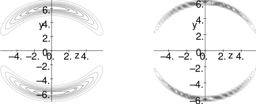
Figure 2: The energy density is distributed in a toroidal region perpendicular to the direction of travel of the spaceship, which is situated at $z_{0}(t)$. We have considered the following values, $v=2$ and $R=6$, with $\sigma=1$ and $\sigma=4$ in $(a)$ and $(b)$, respectively. See the text for more details.

In analogy with the definitions in visser2003 ; Kar2 , one may quantify the “total amount” of energy condition violating matter in the warp bubble, by defining the “volume integral quantifier”

$$M_{\mathrm{warp}}=\int\rho_{\mathrm{warp}}\;d^{3}x=\int T_{\mu\nu}\;U^{\mu}\;U^{\nu}\;d^{3}x=-{v^{2}\over 12}\int\left(\frac{df}{dr}\right)^{2}\;r^{2}\;dr.$$ (10)

This is not the total mass of the spacetime, but it characterizes how much (negative) energy one needs to localize in the walls of the warp bubble. For the specific shape function (2) we can estimate

$$M_{\mathrm{warp}}\approx-v^{2}\;R^{2}\;\sigma,$$ (11)

so that one can readily verify that the energy requirements for the warp bubble scale quadratically with bubble velocity and with bubble size, and inversely as the thickness of the bubble wall LV-CQG .

II.3.2 The violation of the NEC

As before mentioned in the previous chapters, the NEC states that $T_{\mu\nu}\,k^{\mu}\,k^{\nu}\geq 0$, where $k^{\mu}$ is any arbitrary null vector and $T_{\mu\nu}$ is the stress-energy tensor. The NEC for a null vector oriented along the $\pm\hat{z}$ directions takes the following form

$$T_{\mu\nu}\;k^{\mu}\;k^{\nu}=-\frac{v^{2}}{8\pi}\,\left[\left(\frac{\partial f}{\partial x}\right)^{2}+\left(\frac{\partial f}{\partial y}\right)^{2}\right]\pm\frac{v}{8\pi}\left(\frac{\partial^{2}f}{\partial{x}^{2}}+\frac{\partial^{2}f}{\partial{y}^{2}}\right)\,.$$ (12)

Note that if we average over the $\pm\hat{z}$ directions we have the following relation

$${1\over 2}\left[T_{\mu\nu}\;k^{\mu}_{+\hat{z}}\;k^{\nu}_{+\hat{z}}+T_{\mu\nu}\;k^{\mu}_{-\hat{z}}\;k^{\nu}_{-\hat{z}}\right]=-\frac{v^{2}}{8\pi}\,\left[\left(\frac{\partial f}{\partial x}\right)^{2}+\left(\frac{\partial f}{\partial y}\right)^{2}\right],$$ (13)

which is manifestly negative, and implies that the NEC is violated for all $v$. Furthermore, note that even if we do not average, the coefficient of the term linear in $v$ must be nonzero somewhere in the spacetime. Then at low velocities this term will dominate and at low velocities the un-averaged NEC will be violated in either the $+\hat{z}$ or $-\hat{z}$ directions.

II.4 The Quantum Inequality applied to the warp drive

It is of interest to apply the QI to the warp drive spacetimes PfenningF , and rather than deduce the QI in this section, we refer the reader to the Chapter on the Quantum Energy Inequalities. By inserting the energy density, Eq. (8), into the QI, one arrives at the following inequality

$$t_{0}\int_{-\infty}^{+\infty}{v(t)^{2}\over r^{2}}\left({df\over dr}\right)^{2}{dt\over{t^{2}+t_{0}^{2}}}\leq{3\over\rho^{2}\,t_{0}^{4}}\,,$$ (14)

where the quantity $\rho=\left(x^{2}+y^{2}\right)^{1/2}$ is defined for notational convenience.

One may consider that the warp bubble’s velocity is roughly constant, i.e., $v_{s}(t)\approx v_{b}$, by assuming that the time scale of the sampling is sufficiently small compared to the time scale over which the bubble’s velocity is varying. Now, taking into account the small sampling time, the $(t^{2}+t_{0}^{2})^{-1}$ term becomes strongly peaked, so that only a small portion of the geodesic is sampled by the QI integral. Consider also that the observer is situated at the equator of the warp bubble at $t=0$ PfenningF , so that the geodesic is approximated by $x(t)\approx f(\rho)v_{b}t$, and consequently $r(t)=\left[(v_{b}t)^{2}(f(\rho)-1)^{2}+\rho^{2}\right]^{1/2}$.

For simplicity, without a significant loss of generality, and instead of taking into account the Alcubierre form function (2), one may consider a piece-wise continuous form of the shape function given by

$$f_{p.c.}(r)=\left\{\begin{array}[]{c}1\qquad\qquad r<R-{\Delta\over 2}\\ -{1\over\Delta}(r-R-{\Delta\over 2})\qquad R-{\Delta\over 2}<r<R+{\Delta\over 2}\\ 0\qquad\qquad r>R+{\Delta\over 2}\end{array}\right.\,,$$ (15)

where $R$ is the radius of the bubble, and $\Delta$ the bubble wall thickness PfenningF . Note that $\Delta$ is related to the Alcubierre parameter $\sigma$ by setting the slopes of the functions $f(r)$ and $f_{p.c.}(r)$ to be equal at $r=R$, which provides the following relationship $\Delta=\left[1+\tanh^{2}(\sigma R)\right]^{2}/[2\;\sigma\;\tanh(\sigma R)]$.

Note that in the limit of large $\sigma R$ one obtains the approximation $\Delta\simeq 2/\sigma$, so that the QI-bound simplifies to

$$t_{0}\int_{-\infty}^{+\infty}{dt\over(t^{2}+\bar{\beta}^{2})(t^{2}+t_{0}^{2})}\leq{3\Delta^{2}\over v_{b}^{2}\;t_{0}^{4}\;\bar{\beta}^{2}}\,,$$ (16)

where $\bar{\beta}=\rho/\left[{v_{b}(1-f(\rho))}\right]$. Now, evaluating the integral in the left-hand-side yields the following inequality

$${\pi\over 3}\leq{\Delta^{2}\over{v_{b}^{2}\;t_{0}^{4}}}\left[{v_{b}t_{0}\over\rho}(1-f(\rho))+1\right]\;.$$ (17)

It is perhaps important to note that the above inequality is only valid for sampling times on which the spacetime may be considered approximately flat. Considering the Riemann tensor components in an orthonormal frame PfenningF , the largest component is given by

$$|R_{{\hat{t}}{\hat{y}}{\hat{t}}{\hat{y}}}|={3v_{b}^{2}\;y^{2}\over 4\;\rho^{2}}\left[{df(\rho)\over d\rho}\right]^{2}\,,$$ (18)

which yields $r_{\rm min}\equiv 1/\sqrt{|R_{{\hat{t}}{\hat{y}}{\hat{t}}{\hat{y}}}|}\sim 2\Delta/\left({\sqrt{3}}\;v_{b}\right)$, considering $y=\rho$ and the piece-wise continuous form of the shape function. The sampling time must be smaller than this length scale, so that one may define $t_{0}=2\alpha\,\Delta/\left({\sqrt{3}}\;v_{b}\right)$. Assuming $\Delta/\rho\sim v_{b}\,t_{0}/\rho\ll 1$, the term involving $1-f(\rho)$ in Eq. (17) may be neglected, which provides

$$\Delta\leq{3\over 4}\sqrt{3\over\pi}\;{v_{b}\over\alpha^{2}}\,.$$ (19)

Taking a specific value for $\alpha$, for instance, considering $\alpha=1/10$, one obtains

$$\Delta\leq 10^{2}\,v_{b}\;L_{\rm Planck}\,,$$ (20)

where $L_{\rm Planck}$ is the Planck length. Thus, unless $v_{b}$ is extremely large, the wall thickness cannot be much above the Planck scale.

It is also interesting to find an estimate of the total amount of negative energy that is necessary to maintain a warp metric. It was found that the energy required for a warp bubble is on the order of

$$E\leq-3\times 10^{20}\;M_{\rm galaxy}\;v_{b}\;,$$ (21)

which is an absurdly enormous amount of negative energy, roughly ten orders of magnitude greater than the total mass of the entire visible universe PfenningF .

III Linearized warp drive

In this section, we show that there are significant problems that arise even in the warp drive spacetime, even in weak-field regime, and long before strong field effects come into play. Indeed, to ever bring a warp drive into a strong-field regime, any highly-advanced civilization would first have to take it through the weak-field regime LV-CQG . We now construct a more realistic model of a warp drive spacetime where the warp bubble interacts with a finite mass spaceship. To this effect, consider the linearized theory applied to warp drive spacetimes, for non-relativistic velocities, $v\ll 1$.

Consider now a spaceship in the interior of an Alcubierre warp bubble, which is moving along the positive $z$ axis with a non-relativistic constant velocity LV-CQG , i.e., $v\ll 1$. The metric is given by

$$ds^{2} = -dt^{2}+dx^{2}+dy^{2}+\left[dz-v\;f(x,y,z-vt)\,dt\right]^{2}$$ (22)

$$-2\Phi(x,y,z-vt)\,\left[dt^{2}+dx^{2}+dy^{2}+(dz-v\;f(x,y,z-vt)\,dt)^{2}\right]\,,$$

where $\Phi$ is the gravitational field of the spaceship. If $\Phi=0$, the metric (22) reduces to the warp drive spacetime of Eq. (1). If $v=0$, we have the metric representing the gravitational field of a static source.

We consider now the approximation by linearizing in the gravitational field of the spaceship $\Phi$, but keeping the exact $v$ dependence . For this case, the WEC is given by

$$T_{\hat{\mu}\hat{\nu}}\;U^{\hat{\mu}}U^{\hat{\nu}}=\rho-\frac{v^{2}}{32\pi}\left[\left(\frac{\partial f}{\partial x}\right)^{2}+\left(\frac{\partial f}{\partial y}\right)^{2}\right]+O(\Phi^{2})\,,$$ (23)

and assuming the Alcubierre form function, we have

$$T_{\mu\nu}\;U^{\mu}U^{\nu}=\rho-\frac{1}{32\pi}\frac{v^{2}(x^{2}+y^{2})}{r^{2}}\left(\frac{df}{dr}\right)^{2}+O(\Phi^{2})\,.$$ (24)

Using the “volume integral quantifier”, as before, we find the following estimate

$$\int T_{{\mu}{\nu}}\;U^{{\mu}}U^{{\nu}}\;d^{3}x=M_{\rm ship}-v^{2}\;R^{2}\;\sigma+\int O(\Phi^{2})\;d^{3}x\,,$$ (25)

which can be recast in the following form

$$M_{\mathrm{ADM}}=M_{\mathrm{ship}}+M_{\mathrm{warp}}+\int O(\Phi^{2})\;d^{3}x\,.$$ (26)

Now, demanding that the volume integral of the WEC be positive, then we have

$$v^{2}\;R^{2}\;\sigma\leq M_{\rm ship}\,,$$ (27)

which reflects the quite reasonable condition that the net total energy stored in the warp field be less than the total mass-energy of the spaceship itself. Note that this inequality places a powerful constraint on the velocity of the warp bubble. Rewriting this constraint in terms of the size of the spaceship $R_{\mathrm{ship}}$ and the thickness of the warp bubble walls $\Delta=1/\sigma$, we arrive at the following condition

$$v^{2}\leq{M_{\rm ship}\over R_{\mathrm{ship}}}\;{R_{\mathrm{ship}}\;\Delta\over R^{2}}.$$ (28)

For any reasonable spaceship this gives extremely low bounds on the warp bubble velocity.

One may analyse the NEC in a similar manner. Thus, the quantity $T_{{\mu}{\nu}}\,k^{{\mu}}k^{{\nu}}$ is given by

$$T_{\mu\nu}\;k^{{\mu}}k^{{\nu}} = \rho\pm\frac{v}{8\pi}\left(\frac{\partial^{2}f}{\partial x^{2}}+\frac{\partial^{2}f}{\partial y^{2}}\right)-\frac{v^{2}}{8\pi}\left[\left(\frac{\partial f}{\partial x}\right)^{2}+\left(\frac{\partial f}{\partial y}\right)^{2}\right]+O(\Phi^{2})\,.$$ (29)

Considering the “volume integral quantifier”, we may estimate that

$$\int T_{\mu\nu}\;k^{{\mu}}k^{{\nu}}\;d^{3}x=M_{\rm ship}-v^{2}\,R^{2}\,\sigma+\int O(\Phi^{2})\;d^{3}x\,,$$ (30)

which is [to order $O(\Phi^{2})$] the same integral we encountered when dealing with the WEC. In order to avoid that the total NEC violations in the warp field exceed the mass of the spaceship itself, we again demand that

$$v^{2}\;R^{2}\;\sigma\leq M_{\rm ship}\,,$$ (31)

which places an extremely stringent condition on the linearized warp drive spacetime. More specifically, it reflects that that for all conceivably interesting situations the bubble velocity should be absurdly low, and it therefore appears unlikely that, by using this analysis, the warp drive will ever prove to be technologically useful.

Finally, we emphasize that any attempt at building up a “strong-field” warp drive starting from an approximately Minkowski spacetime will inevitably have to pass through a weak-field regime. Taking into account the analysis presented above, we verify that the weak-field warp drives are already so tightly constrained, which implies additional difficulties for developing a “strong field” warp drive .

IV The horizon problem

Shortly after the discovery of the Alcubierre warp drive solution Alcubierre , an interesting feature of the spacetime was found. Namely, an observer on a spaceship cannot create nor control on demand an Alcubierre bubble, with $v>c$, around the ship. Krasnikov . It is easy to understand this, by noting that an observer at the origin (with $t=0$), cannot alter events outside of his future light cone, $|r|\leq t$, with $r=(x^{2}+y^{2}+z^{2})^{1/2}$. In fact, applied to the warp drive, it is a trivial matter to show that points on the outside front edge of the bubble are always spacelike separated from the centre of the bubble.

The analysis is simplified in the proper reference frame of an observer at the centre of the bubble, so that using the transformation $z^{\prime}=z-z_{0}(t)$, the metric is given by

$$ds^{2}=-dt^{2}+dx^{2}+dy^{2}+\left[dz^{\prime}+(1-f)vdt\right]^{2}\,.$$ (32)

Now, consider a photon emitted along the $+Oz$ axis (with $ds^{2}=dx=dy=0$), so that the above metric provides $dz^{\prime}/dt=1-(1-f)v$. If the spaceship is at rest at the center of the bubble, then initially the photon has $dz/dt=v+1$ or $dz^{\prime}/dt=1$ (recall that $f=1$ in the interior of the bubble). However, at a specific point $z^{\prime}=z^{\prime}_{c}$, with $f=1-1/v$, we have $dz^{\prime}/dt=0$ Everett . Once photons reach $z^{\prime}_{c}$, they remain at rest relative to the bubble and are simply carried along with it. This implies that photons emitted in the forward direction by the spaceship never reach the outside edge of the bubble wall, which therefore lies outside the forward light cone of the spaceship. This behaviour is reminiscent of an event horizon. Thus, the bubble thus cannot be created, or controlled, by any action of the spaceship crew, which does not mean that Alcubierre bubbles, if it were possible to create them, could not be used as a means of superluminal travel. It only implies that the actions required to change the metric and create the bubble must be taken beforehand by some observer whose forward light cone contains the entire trajectory of the bubble.

The appearance of an event horizon becomes evident in the 2-dimensional model of the Alcubierre space-time Hiscock ; Clark ; Gonz . Consider that the axis of symmetry coincides with the line element of the spaceship, so that the metric (1), reduces to

$$ds^{2}=-(1-v^{2}f^{2})dt^{2}-2vfdzdt+dz^{2}\,.$$ (33)

For simplicity, we consider a constant bubble velocity, $v(t)=v_{b}$, and $r=[(z-v_{b}t)^{2}]^{1/2}$. Note that the metric components of Eq. (33) only depend on $r$, which may be adopted as a coordinate, so if $z>v_{b}t$, we consider the transformation $r=(z-v_{b}t)$. Using this transformation, $dz=dr+v_{b}\,dt$, the metric (33) takes the following form

$$ds^{2}=-A(r)\left[dt-\frac{v_{b}(1-f(r))}{A(r)}\;dr\right]^{2}+\frac{dr^{2}}{A(r)}\,,$$ (34)

where $A(r)$, denoted by the Hiscock function, is defined by $A(r)=1-v_{b}^{2}\,\left[1-f(r)\right]^{2}$.

Now, it is possible to represent the metric (34) in a diagonal form, using a new time coordinate

$$d\tau=dt-\frac{v_{b}\,\left[1-f(r)\right]}{A(r)}\;dr\,,$$ (35)

so that the metric (34) reduces to a manifestly static form, given by

$$ds^{2}=-A(r)\,d\tau^{2}+\frac{dr^{2}}{A(r)}\,.$$ (36)

The $\tau$ coordinate has an immediate interpretation in terms of an observer on board of a spaceship, namely, $\tau$ is the proper time of the observer, taking into account that $A(r)\rightarrow 1$ in the limit $r\rightarrow 0$. We verify that the coordinate system is valid for any value of $r$, if $v_{b}<1$. If $v_{b}>1$, we have a coordinate singularity and an event horizon at the point $r_{0}$ in which $f(r_{0})=1-1/v_{b}$ and $A(r_{0})=0$.

V Superluminal subway: The Krasnikov tube

It was pointed out above, that an interesting aspect of the warp drive resides in the fact that points on the outside front edge of a superluminal bubble are always spacelike separated from the centre of the bubble. This implies that an observer in a spaceship cannot create nor control on demand an Alcubierre bubble. However, causality considerations do not prevent the crew of a spaceship from arranging, by their own actions, to complete a round trip from the Earth to a distant star and back in an arbitrarily short time, as measured by clocks on the Earth, by altering the metric along the path of their outbound trip. Thus, Krasnikov introduced a metric with an interesting property that although the time for a one-way trip to a distant destination cannot be shortened Krasnikov , the time for a round trip, as measured by clocks at the starting point (e.g. Earth), can be made arbitrarily short, as will be demonstrated below.

V.1 The 2-dimensional Krasnikov solution

The 2-dimensional Krasnikov metric is given by

$$ds^{2} = -(dt-dx)(dt+k(t,x)dx)$$ (37)

$$= -dt^{2}+\left[1-k(x,t)\right]\,dx\,dt+k(x,t)\,dx^{2}\,,$$

where the form function $k(x,t)$ is defined by

$$k(t,x)=1-(2-\delta)\theta_{\varepsilon}(t-x)\left[\theta_{\varepsilon}(x)-\theta_{\varepsilon}(x+\varepsilon-D)\right]\,,$$ (38)

and $\delta$ and $\varepsilon$ are arbitrarily small positive parameters. $\theta_{\varepsilon}$ denotes a smooth monotone function

$$\theta_{\varepsilon}(\xi)=\left\{\begin{array}[]{ll}1,&{\rm if}\;\xi>\varepsilon\,,\\ 0,&{\rm if}\;\xi<0\,.\end{array}\right.$$

One may identify essentially three distinct regions in the Krasnikov two-dimensional spacetime, which is summarized in the following manner.

The outer region:

The outer region is given by the following set

$$\{x<0\}\cup\{x>D\}\cup\{x>t\}\,.$$ (39)

The two time-independent $\theta_{\epsilon}$-functions between the square brackets in Eq. (38) vanish for $x<0$ and cancel for $x>D$, ensuring $k=1$ for all $t$ except between $x=0$ and $x=D$. When this behavior is combined with the effect of the factor $\theta_{\epsilon}(t-x)$, one sees that the metric (37) is flat, i.e., $k=1$, and reduces to Minkowski spacetime everywhere for $t<0$ and at all times outside the range $0<x<D$. Future light cones are generated by the following vectors: $r_{O}=\partial_{t}+\partial_{x}$ and $l_{O}=\partial_{t}-\partial_{x}$.

The inner region:

The inner region is given by the following set

$$\{x<t-\varepsilon\}\cap\{\varepsilon<x<D-\varepsilon\}\,,$$ (40)

so that the first two $\theta_{\epsilon}$-functions in Eq. (38) both equal $1$, while $\theta_{\epsilon}(x+\epsilon-D)=0$, giving $k=\delta-1$ everywhere within this region. This region is also flat, but the light cones are more open, being generated by the following vectors: $r_{I}=\partial_{t}+\partial_{x}$ and $l_{I}=-(1-\delta)\partial_{t}-\partial_{x}$.

The transition region:

The transition region is a narrow curved strip in spacetime, with width $\sim\varepsilon$. Two spatial boundaries exist between the inner and outer regions. The first lies between $x=0$ and $x=\varepsilon$, for $t>0$. The second lies between $x=D-\varepsilon$ and $x=D$, for $t>D$. It is possible to view this metric as being produced by the crew of a spaceship, departing from point $A$ ($x=0$), at $t=0$, travelling along the $x$-axis to point $B$ ($x=D$) at a speed, for simplicity, infinitesimally close to the speed of light, therefore arriving at $B$ with $t\approx D$.

Thus, the metric is modified by changing $k$ from $1$ to $\delta-1$ along the $x$-axis, in between $x=0$ and $x=D$, leaving a transition region of width $\sim\varepsilon$ at each end for continuity. However, as the boundary of the forward light cone of the spaceship at $t=0$ is $|x|=t$, it is not possible for the crew to modify the metric at an arbitrary point $x$ before $t=x$. This fact accounts for the factor $\theta_{\varepsilon}(t-x)$ in the metric, ensuring a transition region in time between the inner and outer region, with a duration of $\sim\varepsilon$, lying along the wordline of the spaceship, $x\approx t$. The geometry is shown in the $(x,t)$ plane in Figure 3.

Figure 3: The plot depicts the Krasnikov spacetime in the $(x,t)$ plane, where the vertical lines $A$ and $B$ are the world lines of the stars $A$ and $B$, respectively. The world line of the spaceship is approximately represented by the line segment $AB$. See the text for more details.

V.2 Superluminal travel within the Krasnikov tube

The factored form of the metric (37), for $ds^{2}=0$, provides some interesting properties of the spacetime with $\delta-1\leq k\leq 1$. Note that the two branches of the forward light cone in the $(t,x)$ plane are given by $dx/dt=1$ and $dx/dt=-k$. As $k$ becomes smaller and then negative, the slope of the left-hand branch of the light cone becomes less negative and then changes sign. This implies that the light cone along the negative $x$-axis opens out, as depicted in Figure 4).

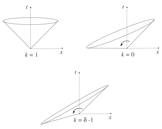
Figure 4: Forward light cones in the 2-dimensional Krasnikov spacetime for $k=1$, $k=0$ and $k=\delta-1$.

The inner region, with $k=\delta-1$, is flat because the metric (37) may be cast into the Minkowski form, applying the following coordinate transformations

$$dt^{\prime}=dt+\left(\frac{\delta}{2}-1\right)dx\,,\qquad dx^{\prime}=\left(\frac{\delta}{2}\right)dx\,,$$ (41)

and one verifies that the transformation is singular at $\delta=0$, i.e., $k=-1$. Note that the left branch of the region is given by $dx^{\prime}/dt^{\prime}=-1$.

From the above analysis, one may easily deduce the following expression

$$\frac{dt}{dt^{\prime}}=1+\left(\frac{2-\delta}{\delta}\right)\frac{dx^{\prime}}{dt^{\prime}}\,.$$ (42)

For an observer moving along the positive $x^{\prime}$ and $x$ directions, with $dx^{\prime}/dt^{\prime}<1$, we have $dt^{\prime}>0$ and consequently $dt>0$, if $0<\delta\leq 2$. However, if the observer is moving sufficiently close to the left branch of the light cone, given by $dx^{\prime}/dt^{\prime}=-1$, Eq. (42) provides us with $dt/dt^{\prime}<0$, for $\delta<1$. Therefore we have $dt<0$, which means that the observer traverses backward in time, as measured by observers in the outer region, with $k=1$.

The superluminal travel analysis is as follows. Consider a spaceship departing from star $A$ and arriving at star $B$, at the instant $t\approx D$. Along this journey, the crew of the spaceship modify the metric, so that $k\approx-1$, for simplicity, along the trajectory. Now imagine that the spaceship returns to star $A$, travelling with a velocity arbitrarily close to the speed of light, i.e., $dx^{\prime}/dt^{\prime}\approx-1$. Therefore, from Eq. (41), one obtains the following relation

$$v_{\rm return}=\frac{dx}{dt}\approx-\frac{1}{k}=\frac{1}{1-\delta}\approx 1$$ (43)

and $dt<0$, for $dx<0$. The return trip from star $B$ to $A$ is done in an interval of $\Delta t_{\rm return}=-D/v_{\rm return}=D/(\delta-1)$. Note that the total interval of time, measured at $A$, is given by $T_{A}=D+\Delta t_{\rm return}=D\delta$. For simplicity, consider $\varepsilon$ negligible, so that superluminal travel is implicit, as $|\Delta t_{\rm return}|<D$, if $0<\delta<1$, i.e., we have a spatial spacetime interval between $A$ and $B$. Now, $T_{A}$ is always positive, but may attain a value arbitrarily close to zero, for an appropriate choice of $\delta$.

Note that for the case $\delta<1$, it is always possible to choose an allowed value of $dx^{\prime}/dt^{\prime}$ for which $dt/dt^{\prime}=0$, meaning that the return trip is instantaneous as seen by observers in the external region. This follows easily from Eq. (42), which implies that $dt/dt^{\prime}=0$ when $dx^{\prime}/dt^{\prime}$ satisfies $dx^{\prime}/dt^{\prime}=-\delta/(2-\delta)$, which lies between $0$ and $-1$ for $0<\delta<1$.

V.3 The 4-dimensional generalization

Shortly after the Krasnikov two-dimensional solution, the analysis was generalized to four dimensions by Everett and Roman Everett , who denoted the solution as the Krasnikov tube. The latter four-dimensional modification of the metric begins along the path of the spaceship, which is moving along the $x$-axis, and occurs at the position $x$, at time $t\approx x$, which is the time of passage of the spaceship. Everett and Roman also assumed that the disturbance in the metric propagated radially outward from the $x$-axis, so that causality guarantees that at time $t$ the region in which the metric has been modified cannot extend beyond $\rho=t-x$, where $\rho={(y^{2}+z^{2})}^{1/2}$. The modification in the metric was also assumed to not extend beyond some maximum radial distance $\rho_{max}\ll D$ from the $x$-axis.

Thus, the metric in the 4-dimensional spacetime, written in cylindrical coordinates, is given by Everett

$$ds^{2}=-dt^{2}+[1-k(t,x,\rho)]\,dx\,dt+k(t,x,\rho)dx^{2}+d\rho^{2}+\rho^{2}d\phi^{2}\,,$$ (44)

where the four-dimensional generalization of the Krasnikov form function is given by

$$k(t,x,\rho)=1-(2-\delta)\theta_{\varepsilon}(\rho_{max}-\rho)\theta_{\varepsilon}(t-x-\rho)[\theta_{\varepsilon}(x)-\theta_{\varepsilon}(x+\varepsilon-D)]\,.$$ (45)

For $t\gg D+\rho_{max}$ one has a tube of radius $\rho_{max}$ centered on the $x$-axis, within which the metric has been modified. I is this structure that is denoted by the Krasnikov tube, and contrary to the Alcubierre spacetime metric, the metric of the Krasnikov tube is static, once it has been created.

The stress-energy tensor element $T_{tt}$ given by

$$T_{tt}=\frac{1}{32\pi(1+k)^{2}}\left[-\frac{4(1+k)}{\rho}\frac{\partial k}{\partial\rho}+3\left(\frac{\partial k}{\partial\rho}\right)^{2}-4(1+k)\frac{\partial^{2}k}{\partial\rho^{2}}\right]\,,$$ (46)

can be shown to be the energy density measured by a static observer Everett , and violates the WEC in a certain range of $\rho$, i.e., $T_{\mu\nu}U^{\mu}U^{\nu}<0$. To this effect, consider the energy density in the middle of the tube and at a time long after it’s formation, i.e., $x=D/2$ and $t\gg x+\rho+\varepsilon$, respectively. In this region we have $\theta_{\varepsilon}(x)=1$, $\theta_{\varepsilon}(x+\varepsilon-D)=0$ and $\theta_{\varepsilon}(t-x-\rho)=1$. With this simplification the form function (45) reduces to

$$k(t,x,\rho)=1-(2-\delta)\theta_{\varepsilon}(\rho_{max}-\rho)\,.$$ (47)

A useful form for $\theta_{\varepsilon}(\xi)$ Everett is given by

$$\theta_{\varepsilon}(\xi)=\frac{1}{2}\left\{\tanh\left[2\left(\frac{2\xi}{\varepsilon}-1\right)\right]+1\right\}\,,$$ (48)

so that the form function (47) yields

$$k=1-\left(1-\frac{\delta}{2}\right)\left\{\tanh\left[2\left(\frac{2\xi}{\varepsilon}-1\right)\right]+1\right\}\,.$$ (49)

Choosing the following values for the parameters: $\delta=0.1$, $\varepsilon=1$ and $\rho_{max}=100\varepsilon=100$, the negative character of the energy density is manifest in the immediate inner vicinity of the tube wall, as shown in Figure 5.

Figure 5: Graph of the energy density, $T_{tt}$, as a function of $\rho$ at the middle of the Krasnikov tube, $x=D/2$, and long after it’s formation, $t\gg x+\rho+\varepsilon$. We consider the following values for the parameters: $\delta=0.1$, $\varepsilon=1$ and $\rho_{max}=100\varepsilon=100$. See the text for details.

VI Closed timelike curves

VI.1 The warp drive

Consider a hypothetical spaceship immersed within a warp bubble, moving along a timelike curve, with an arbitrary value of $v(t)$. Due to the latter, the metric of the warp drive permits superluminal travel, which raises the possibility of the existence of CTCs. Although the solution deduced by Alcubierre by itself does not possess CTCs, Everett demonstrated that these are created by a simple modification of the Alcubierre metric Everett , by applying a similar analysis as is carried out using tachyons.

The modified metric takes the form

$$ds^{2}=-dt^{2}+dx^{2}+dy^{2}+(dz-vfdt)^{2}\,,$$ (50)

with $v(t)=dz_{0}(t)/dt$ and $r(t)=[(z-z_{0})^{2}+(y-y_{0})^{2}+z^{2}]^{1/2}$. As in Section II.1 spacetime is flat in the exterior of a warp bubble with radius $R$, which now in the modified is centered in $(0,y_{0},z_{0}(t))$. The bubble moves with a velocity $v$, on a trajectory parallel to the $z$-axis. Consider, for simplicity, the form function given by Eq. (2). We shall also impose that $y_{0}\gg R$, so that the form function is negligible, i.e., $f(y_{0})\approx 0$.

Now, consider two stars, $S_{1}$ and $S_{2}$, at rest in the coordinate system of the metric (50), and located on the $z$-axis at $t=0$ and $t=D$, respectively. The metric along the $z$-axis is Minkowskian as $y_{0}\gg R$. Therefore, a light beam emitted at $S_{1}$, at $t=0$, moving along the $z$-axis with $dz/dt=1$, arrives at $S_{2}$ at $t=D$. Suppose that the spaceship initially starts off from $S_{1}$, with $v=0$, moving off to a distance $y_{0}$ along the $y-$axis and neglecting the time it needs to cover $y=0$ to $y=y_{0}$. At $y_{0}$, it is then subject to a uniform acceleration, $a$, along the the $z-$axis for $0<z<D/2$, and $-a$ for $D/2<z<D$. The spaceship will arrive at the spacetime event $S_{2}$ with coordinates $z=D$ and $t=2\sqrt{D/a}\equiv T$. Once again, the time required to travel from $y=y_{0}$ to $y=0$ is negligible.

The separation between the two events, departure and arrival, is $D^{2}-T^{2}=D^{2}(1-4/(aD)$ and will be spatial if $a>4/D$ is verified. In this case, the spaceship will arrive at $S_{2}$ before the light beam, if the latter’s trajectory is a straight line, and both departures are simultaneous from $S_{1}$. Inertial observers situated in the exterior of the spaceship, at $S_{1}$ and $S_{2}$, will consider the spaceship’s movement as superluminal, since the distance $D$ is covered in an interval $T<D$. However, the spaceship’s wordline is contained within it’s light cone. The worldline of the spaceship is given by $z=vt$, while it’s future light cone is given by $z=(v\pm 1)t$. The latter relation can easily be inferred from the null condition, $ds^{2}=0$.

Since the quadri-vector with components $(T,0,0,D)$ is spatial, the temporal order of the events, departure and arrival, is not well-defined. Introducing new coordinates, $(t^{\prime},x^{\prime},y^{\prime},z^{\prime})$, obtained by a Lorentz transformation, with a boost $\beta$ along the $z$-axis. The arrival at $S_{2}$ in the $(t^{\prime},x^{\prime},y^{\prime},z^{\prime})$ coordinates correspond to

$$T^{\prime}=\gamma(2\sqrt{D/a}-\beta D)\,,\qquad Z^{\prime}=\gamma(D-2\sqrt{D/a})\,,$$ (51)

with $\gamma=(1-\beta^{2})^{-1/2}$. The events, departure and arrival, will be simultaneous if $a=4/(\beta^{2}D)$. The arrival will occur before the departure if $T^{\prime}<0$, i.e.,

$$a>\frac{4}{\beta^{2}D}\,.$$ (52)

The fact that the spaceship arrives at $S_{2}$ with $t^{\prime}<0$, does not by itself generate CTCs. Consider the metric (50), substituting $z$ and $t$ by $\Delta z^{\prime}=z^{\prime}-Z^{\prime}$ and $\Delta t^{\prime}=t^{\prime}-T^{\prime}$, respectively; $v(t)$ by $-v(t)$; $a$ by $-a$; and $y_{0}$ by $-y_{0}$. This new metric describes a spacetime in which an Alcubierre bubble is created at $t^{\prime}=T^{\prime}$, which moves along $y=-y_{0}$ and $x=0$, from $S_{1}$ to $S_{2}$ with a velocity $v^{\prime}(t^{\prime})$, and subject to an acceleration $a^{\prime}$. For observers at rest relatively to the coordinates $(t^{\prime},x^{\prime},y^{\prime},z^{\prime})$, situated in the exterior of the second bubble, it is identical to the bubble defined by the metric (50), as it is seen by inertial observers at rest at $S_{1}$ and $S_{2}$. The only differences reside in a change of the origin, direction of movement and possibly of the value of acceleration. The stars, $S_{1}$ and $S_{2}$, are st rest in the coordinate system of the metric (50), and in movement along the negative direction of the $z$-axis with velocity $\beta$, relatively to the coordinates $(t^{\prime},x^{\prime},y^{\prime},z^{\prime})$. The two coordinate systems are equivalent due to the Lorentz invariance, so if the first is physically realizable, then so is the second. In the new metric, by analogy with Eq. (50), we have $d\tau=dt^{\prime}$, i.e., the proper time of the observer, on board of the spaceship, travelling in the centre of the second bubble, is equal to the time coordinate, $t^{\prime}$. The spaceship will arrive at $S_{1}$ in the temporal and spatial intervals given by $\Delta t^{\prime}>0$ and $\Delta z^{\prime}<0$, respectively. As in the analysis of the first bubble, the separation between the departure, at $S_{2}$, and the arrival $S_{1}$, will be spatial if the analogous relationship of Eq. (52) is verified. Therefore, the temporal order between arrival and departure is also not well-defined. As will be verified below, when $z$ and $z^{\prime}$ decrease and $t^{\prime}$ increases, $t$ will decrease and a spaceship will arrive at $S_{1}$ at $t<T$. In fact, one may prove that it may arrive at $t<0$.

Since the objective is to verify the appearance of CTCs, in principle, one may proceed with some approximations. For simplicity, consider that $a$ and $a^{\prime}$, and consequently $v$ and $v^{\prime}$ are enormous, so that $T\ll D$ and $\Delta t^{\prime}\ll-\Delta z^{\prime}$. In this limit, we obtain the approximation $T\approx 0$, i.e., the journey of the first bubble from $S_{1}$ to $S_{2}$ is approximately instantaneous. Consequently, taking into account the Lorentz transformation, we have $Z^{\prime}\approx\gamma D$ and $T^{\prime}\approx-\gamma\beta D$. To determine $T_{1}$, which corresponds to the second bubble at $S_{1}$, consider the following considerations: since the acceleration is enormous, we have $\Delta t^{\prime}\approx 0$ and $\Delta t=T_{1}-T\approx T_{1}$, therefore $\Delta z=-D\approx\gamma\Delta z^{\prime}$ and $\Delta t\approx\gamma\beta\Delta z^{\prime}$, from which one concludes that

$$T_{1}\approx-\beta D<0\,.$$ (53)

VI.2 The Krasnikov tube

As mentioned above, for superluminal speeds the warp drive metric has a horizon so that an observer in the center of the bubble is causally separated from the front edge of the bubble. Therefore he/she cannot control the Alcubierre bubble on demand. In order to address this problem, Krasnikov proposed a two-dimensional metric Krasnikov , which was later extended to a four-dimensional model Everett , as outlined in Section V. A two-dimensional Krasnikov tube does not generate CTCs. But the situation is quite different in the 4-dimensional generalization. Using two such tubes it is a simple matter, in principle, to generate CTCs Everett:1995nn . The analysis is similar to that of the warp drive, so that it will be treated in summary.

Imagine a spaceship travelling along the $x$-axis, departing from a star, $S_{1}$, at $t=0$, and arriving at a distant star, $S_{2}$, at $t=D$. An observer on board of the spaceship constructs a Krasnikov tube along the trajectory. It is possible for the observer to return to $S_{1}$, travelling along a parallel line to the $x$-axis, situated at a distance $\rho_{0}$, so that $D\gg\rho_{0}\gg 2\rho_{max}$, in the exterior of the first tube. On the return trip, the observer constructs a second tube, analogous to the first, but in the opposite direction, i.e., the metric of the second tube is obtained substituting $x$ and $t$, for $X=D-x$ and $T=t-D$, respectively in eq. (44). The fundamental point to note is that in three spatial dimensions it is possible to construct a system of two non-overlapping tube separated by a distance $\rho_{0}$.

After the construction of the system, an observer may initiate a journey, departing from $S_{1}$, at $x=0$ and $t=2D$. One is only interested in the appearance of CTCs in principle, therefore the following simplifications are imposed: $\delta$ and $\varepsilon$ are infinitesimal, and the time to travel between the tubes is negligible. For simplicity, consider the velocity of propagation close to that of light speed. Using the second tube, arriving at $S_{2}$ at $x=D$ and $t=D$, then travelling through the first tube, the observer arrives at $S_{1}$ at $t=0$. The spaceship has completed a CTC, arriving at $S_{1}$ before it’s departure.

VII Summary and Conclusion

In this chapter, we have seen how warp drive spacetimes can be used as gedanken-experiments to probe the foundations of general relativity. Though they are useful toy models for theoretical investigations, we emphasize that as potential technology they are greatly lacking. We have verified that exact solutions of the warp drive spacetimes necessarily violate the classical energy conditions, and continue to do so for arbitrarily low warp bubble velocity. Thus, the energy condition violations in this class of spacetimes is generic to the form of the geometry under consideration and is not simply a side-effect of the superluminal properties. Furthermore, by taking into account the notion of the “volume integral quantifier”, we have also verified that the “total amount” of energy condition violating matter in the warp bubble is negative.

Using linearized theory, a more realistic model of the warp drive spacetime was constructed where the warp bubble interacts with a finite mass spaceship. The energy conditions were determined to first and second order of the warp bubble velocity, which safely ignores the causality problems associated with “superluminal” motion. A fascinating feature of these solutions resides in the fact that such a spacetime appear to be examples of a “reactionless” drives, where the warp bubble moves by interacting with the geometry of spacetime instead of expending reaction mass, and the spaceship is simply carried along with it. Note that in linearized theory the spaceship can be treated as a finite mass object placed within the warp bubble. It was verified that in this case, the “total amount” of energy condition violating matter, the “net” negative energy of the warp field, must be an appreciable fraction of the positive mass of the spaceship carried along by the warp bubble. This places an extremely stringent condition on the warp drive spacetime, in that the bubble velocity should be absurdly low. Finally, we point out that any attempt at building up a “strong-field” warp drive starting from an approximately Minkowski spacetime will inevitably have to pass through a weak-field regime. Since the weak-field warp drives are already so tightly constrained, the analysis of the linearized warp drive implies additional difficulties for developing a “strong field” warp drive.

Furthermore, we have shown that shortly after the discovery of the Alcubierre warp drive solution it was found that an observer on a spaceship cannot create nor control on demand a superluminal Alcubierre bubble, due to a feature that is reminiscent of an event horizon. Thus, the bubble cannot be created, nor controlled, by any action of the spaceship crew. We emphasize that this does not mean that Alcubierre bubbles could not be theoretically used as a means of superluminal travel, but that the actions required to change the metric and create the bubble must be taken beforehand by an observer whose forward light cone contains the entire trajectory of the bubble. To contour this difficulty, Krasnikov introduced a two-dimensional metric in which the time for a round trip, as measured by clocks at the starting point (e.g. Earth), can be made arbitrarily short. This metric was generalized the analysis to four dimensions, denoting the solution as the Krasnikov tube. It was also shown that this solution violates the energy conditions is specific regions of spacetime. Finally, it was shown that these spacetimes induce closed timelike curves.

References

- (1) M. S. Morris and K. S. Thorne, “Wormholes in spacetime and their use for interstellar travel: A tool for teaching General Relativity,” Am. J. Phys. 56, 395 (1988).
- (2) M. Visser, Lorentzian Wormholes: From Einstein to Hawking (American Institute of Physics, New York, 1995).
- (3) M. Alcubierre, “The warp drive: hyper-fast travel within general relativity,” Class. Quant. Grav. 11, L73-L77 (1994).
- (4) M. Visser, B. Bassett and S. Liberati, “Perturbative superluminal censorship and the null energy condition,” Proceedings of the Eighth Canadian Conference on General Relativity and Relativistic Astrophysics (AIP Press) (1999).
- (5) M. Visser, B. Bassett and S. Liberati, “Superluminal censorship,” Nucl. Phys. Proc. Suppl. 88, 267-270 (2000).
- (6) K. Olum, “Superluminal travel requires negative energy density,” Phys. Rev. Lett, 81, 3567-3570 (1998).
- (7) C. Barcelo and M. Visser, “Twilight for the energy conditions?,” Int. J. Mod. Phys. D 11, 1553 (2002).
- (8) C. Barcelo and M. Visser, “Scalar fields, energy conditions, and traversable wormholes,” Class. Quant. Grav. 17, 3843 (2000).
- (9) C. Barcelo and M. Visser, “Traversable wormholes from massless conformally coupled scalar fields,” Phys. Lett. B 466, 127 (1999).
- (10) A. G. Riess et al., “Type Ia Supernova Discoveries at From the Hubble Space Telescope: Evidence for Past Deceleration and Constraints on Dark Energy Evolution,” Astrophys. J. 607, 665-687 (2004).
- (11) M. Visser, “Jerk, snap, and the cosmological equation of state,” Class. Quant. Grav. 21, 2603 (2004).
- (12) R. R. Caldwell, M. Kamionkowski and N. N. Weinberg, “Phantom Energy and Cosmic Doomsday,” Phys. Rev. Lett. 91 071301 (2003).
- (13) S. V. Krasnikov, “Hyper-fast Interstellar Travel in General Relativity,” Phys. Rev. D 57, 4760 (1998) [arXiv:gr-qc/9511068].
- (14) A. E. Everett and T. A. Roman, “A Superluminal Subway: The Krasnikov Tube,” Phys. Rev. D 56, 2100 (1997).
- (15) J. Natário, “Warp drive with zero expansion,” Class. Quant. Grav. 19, 1157, (2002).
- (16) L. H. Ford and T. A. Roman, “Averaged energy conditions and quantum inequalities,” Phys. Rev. D 51, 4277 (1995).
- (17) L. H. Ford and T. A. Roman, “Quantum field theory constrains traversable wormhole geometries,” Phys. Rev. D 53, 5496 (1996).
- (18) M. J. Pfenning and L. H. Ford, “The unphysical nature of warp drive,” Class. Quant. Grav. 14, 1743, (1997).
- (19) C. Van Den Broeck, “A ’Warp drive’ with reasonable total energy requirements,” Class. Quant. Grav. 16, 3973 (1999).
- (20) P. Gravel and J. Plante, “Simple and double walled Krasnikov tubes: I. Tubes with low masses,” Class. Quant. Grav. 21, L7, (2004).
- (21) P. Gravel, “Simple and double walled Krasnikov tubes: II. Primordial microtubes and homogenization,” Class. Quant. Grav. 21, 767, (2004).
- (22) F. S. N. Lobo and M. Visser, “Fundamental limitations on ‘warp drive’ spacetimes,” Class. Quant. Grav. 21, 5871 (2004).
- (23) J. W. York, “Kinematic and dynamics of general relativity”, in L. L. Smarr editor, Sources of gravitational radiation”, Cambridge University Press, UK, 1979, pp. 83-126.
- (24) M. Alcubierre, Introduction to 3+1 numerical relativity (Oxford University Press, UK, 2008).
- (25) M. Visser, S. Kar and N. Dadhich, “Traversable wormholes with arbitrarily small energy condition violations,” Phys. Rev. Lett. 90, 201102 (2003).
- (26) S. Kar, N. Dadhich and M. Visser, “Quantifying energy condition violations in traversable wormholes,” Pramana 63, 859-864 (2004).
- (27) W. A. Hiscock, “Quantum effects in the Alcubierre warp drive spacetime,” Class. Quant. Grav. 14, L183 (1997).
- (28) C. Clark, W. A. Hiscock and S. L. Larson, “Null geodesics in the Alcubierre warp drive spacetime: the view from the bridge,” Class. Quant. Grav. 16, 3965 (1999).
- (29) P. F. González-Díaz, “On the warp drive space-time,” Phys. Rev. D 62, 044005 (2000).
- (30) A. E. Everett, “Warp drive and causality,” Phys. Rev. D 53, 7365 (1996).