Dory: Overcoming Barriers to Computing Persistent Homology

Abstract

Persistent homology (PH) is an approach to topological data analysis (TDA) that computes multi-scale topologically invariant properties of high-dimensional data that are robust to noise. While PH has revealed useful patterns across various applications, computational requirements have limited applications to small data sets of a few thousand points. We present Dory, an efficient and scalable algorithm that can compute the persistent homology of large data sets. Dory uses significantly less memory than published algorithms and also provides significant reductions in the computation time compared to most algorithms. It scales to process data sets with millions of points. As an application, we compute the PH of the human genome at high resolution as revealed by a genome-wide Hi-C data set. Results show that the topology of the human genome changes significantly upon treatment with auxin, a molecule that degrades cohesin, corroborating the hypothesis that cohesin plays a crucial role in loop formation in DNA.

Keywords T

opological data analysis, multi scale, algorithm, large data sets, genome structure

1 Introduction

The ever increasing availability of scientific data necessitates development of mathematical algorithms and computational tools that yield testable predictions or give mechanistic insights into model systems underlying the data. The utility of these algorithms is determined by the validity of their theoretical foundations, the generality of their applications, their ability to deal with noisy, high-dimensional, and incomplete data, and the computational scalability. Persistent homology (PH), a mathematically rigorous approach to topological data analysis (TDA), finds patterns in high-dimensional data that are robust to noise, providing a multi-scale overview of the topology of the data.

For example, consider a point-cloud data set of 3000 points (Figure 1(a)). The three rectangles (Figure 1(b)) show different scales of observation of the data. At the small spatial scale (rectangle 1), we do not see a discernible pattern, at a larger scale (rectangle 2), two holes with a distinct pattern appear, and increasing the scale further reveals a third distinct pattern, the large hole at the center (rectangle 3). For this data set, PH will compute that there are three groups of topologically distinct features. It will also indicate the scale at which they emerge. However, this analysis comes at a high computational cost that has limited the applicability of PH to very small data sets. To introduce these extant computational limitations, we briefly introduce some terminology. A general and detailed exposition on persistent homology can be found in Edelsbrunner and Harer (2008).

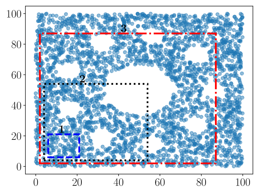
(a) We zoom in at three different scales—rectangle 1, 2, and 3.

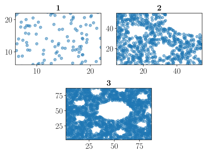
(b) New patterns emerge at different scales.

Figure 1: A simulated data set with 3000 points.

To formalize the notion of topology of a discrete data set, a collection of so-called simplices is defined from the data set as follows: An $n$-simplex is a set of $n+1$ points and is said to have dimension $n$ (dim-$n$). Figure 2(a) shows different ways to interpret a simplex—as a mathematical set, graphical object, or geometric object—in different dimensions. The boundary of an $n$-simplex $\sigma,$ denoted $\partial\sigma,$ is the set of all $(n-1)$-simplices contained in the simplex. The coboundary of an $n$-simplex $\sigma,$ denoted by $\delta\sigma,$ is the set of all $(n+1)$-simplices $\omega$ such that $\sigma\in\partial\omega.$ A collection of simplices is called a complex. Figure 2(b) shows examples of coboundaries and complexes. Contraction can be visualized as a continuous deformation of a simplex to a point. Non-contractible topological structures correspond to obstructions to such a contraction, suggesting the possible existence of a feature in the data.

A hole in dim-$d$ is a complex that has a non-contractible boundary in dim-$(d-1).$ The complex $D^{\prime}$ in Figure 2(b) contains the simplex $\{a,b,c\},$ and hence its boundary $\partial\{a,b,c\}=\{\{a,b\},\{b,c\},\{c,a\}\}$ will contract in dim-1. On the other hand, since the complex $D$ does not contain $\{a,b,c\},$ its boundary $\partial\{a,b,c\}$ cannot contract in dim-1. Hence, $D$ contains a non-contractible structure or a hole. These non-contractible structures in dim-$d$ define the homology group for dim-$d,$ denoted by H${}_{d},$ partitioned into equivalence classes that are related by contractible simplices. For example, the homology group H₁ of the complex $D$ has one equivalence class. The non-contractible structures in H₀ can be mapped to path-connected components when the complex is viewed as a discrete graph. Those in H₁ can be mapped to holes on the surface of the triangulation of the point cloud, but are more commonly referred as loops, indicative of one dimensional boundaries around the holes. In H₂ they can be thought of as voids in an embedding of the triangulation in a three-dimensional metric space, and sets of triangular faces will define their boundaries.

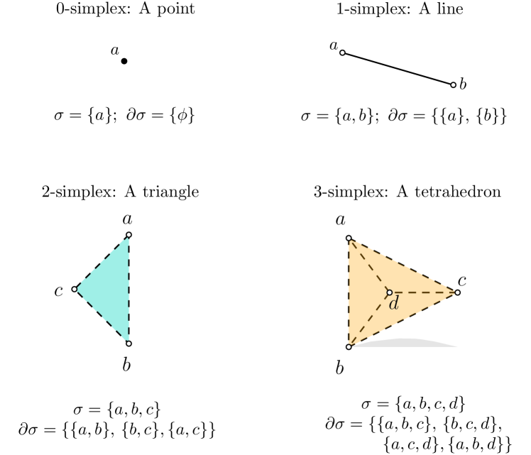
(a) Simplices

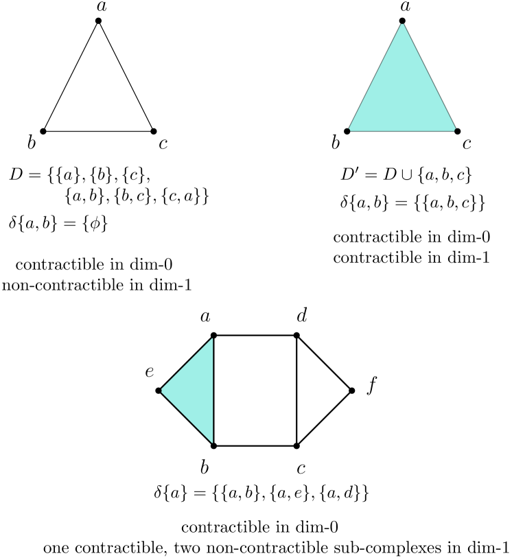
(b) Contractible and non-contractible structures in complexes.

Figure 2: Simplices form the building blocks for defining a topological space on discrete data set, simplicial topology.

To give a multi-scale overview, PH tracks changes in the homology groups as the scale of observation changes. We see that the collection of simplices in the data set, otherwise known as the complex of the data set, changes at different spatial scales as its construction is based on pairwise distances in the discrete data set. The example (Figure 3) shows 4 points in a metric space, with the numbers between two points representing the spatial pairwise distances ($d(x,y)$). At any given scale of observation $\tau$ we build a complex with all of the 1-simplices $\{a,b\}$ such that $d(x,y)\leq\tau.$ Additionally, to compute H${}_{d},$ all $(d+1)$-simplices whose boundary is in the complex are also added to it. This results in a factorial increase in the number of simplices to consider in the complex scaling as the number of points in the data set is raised to a power two larger than the dimension of the homology group. In Figure 3, when $\tau=0,$ there are 4 points or 0-simplices. These are indexed arbitrarily from $\sigma_{0}$ to $\sigma_{3}.$ Starting from $D_{0}=\{\sigma_{0}\},$ we define a sequence of complexes $D_{0}\subset D_{1}\subset...\subset D_{n}$ such that $D_{i}=D_{i-1}\cup\{\sigma_{i}\}.$ At $\tau=0,$ we have $D_{3}=\{\sigma_{0},\sigma_{1},\sigma_{2},\sigma_{3}\}.$ As $\tau$ increases, more simplices are added to the complex, and the sequence $(D_{0},...,D_{11})$ can be computed for this example. Simplices that are added to the complex at the same value of $\tau$ can be ordered arbitrarily relative to each other. This sequence of complexes is called the Vietoris-Rips filtration.

For every complex in the VR-filtration, we compute the homology groups and record changes in them as we process complexes in the filtration. For example, there is the birth of a hole (equivalently, a loop) in H₁ when $\sigma_{8}$ is added, which contracts or dies when $\sigma_{11}$ is added. Birth-death pairs are called persistence pairs, and they are plotted as a function of the scale, $\tau.$ In our example, the persistence pair is $(\sigma_{8},\sigma_{11})$ in H${}_{1}.$ These pairs gives us persistence diagrams (PD), one for every H_d that is computed. The persistence diagram corresponding to H₁ for this example will contain exactly $(2.5,2.75),$ since $\sigma_{8}$ is added at $\tau=2.5$ and $\sigma_{11}$ is added at $\tau=2.75.$ The persistence diagram for the example in Figure 1(a) is shown in Figure 4(b).

It has been shown that the same persistence diagram can be obtained by computing cohomology groups, denoted by H${}^{*}_{d}.$ If $(\sigma,\tau)$ is a persistence pair in H${}_{d},$ then $(\tau,\sigma)$ is a persistence pair in H${}^{*}_{d},$ and consequently, $\mid\text{H}_{d}\mid=\mid\text{H}^{*}_{d}\mid.$ Moreover, the algorithms that compute the persistence pairs of H_d can also be used to compute the persistence pairs of H${}_{d}^{*}$ by applying them to the coboundaries of the complexes in the filtration (De Silva et al., 2011).

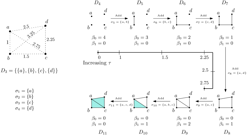
Figure 3: Topological features—number of components ($\beta_{0}$) and holes ($\beta_{1}$)—change as the scale of observation ($\tau$) changes.

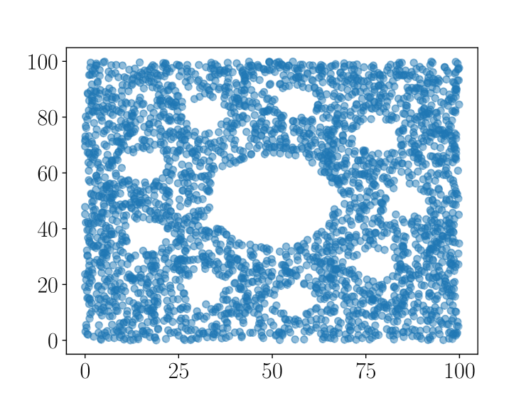
(a) Scatter plot from Figure 1(a).

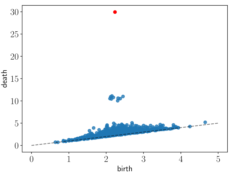
(b) H₁ PD shows that there are three topologically distinct groups of features that emerge across multiple scales. The red dot corresponds to the large hole at the center.

Figure 4: Scatter plot of the data set and its H₁ persistence diagram.

As discussed above, computing H₂ across all scales of a data set requires storing and processing all 3-simplices, that is, $O(n^{4})$ simplices. Even for a small data set with $n=500$ data points, the number of 3-simplices is $500\choose 4$ $=2573031125,$ indicative of the memory required to represent the filtration in the computer. Different methods have been developed for storing this information. We compare our algorithm with three software packages—Gudhi, Ripser, and Eirene. Gudhi represents the filtration using a simplex tree (Boissonnat and Maria, 2014), and Ripser (Bauer, 2019) represents a simplex using combinatorial indexing. For large data sets, creating a simplex tree for the entire filtration a priori can require memory up to $O(n^{4}),$ and indexing simplices using combinatorial indexing overflows the bounds of integer data types in most computer architectures. Therefore, both these methods cannot process data sets with large numbers of points. Eirene uses matroid theory that takes more memory than Ripser and, in some cases, more memory than Gudhi. All packages failed to compute PH for at least one data set in our experiments. None were able to process the data set of interest to us, the conformations of the human genome, because of such practical limitations. As PH computation requires processing a combinatorially large number of simplices as well, any method for reducing memory requirements had better not be accompanied by an inordinate increase in computation time either.

Due to these computational difficulties, published algorithms have been practically limited to computing topological features up to and including H${}_{2}.$ This still allows for applications of PH to a large class of data sets in the physical sciences or to low-dimensional embeddings of high-dimensional data. Therefore, we focus on computing topological features only up to and including the first three dimensions. We take advantage of this restriction to devise a new way to store information and new algorithms to process it, resulting in a reduction in memory requirements by orders of magnitude accompanied with reduced computation time in almost all our test cases.

The two meter long human DNA fits into a nucleus with an average diameter of 10 $\mu$m by folding into a complex, facilitated by many proteins which play functional and structural roles (Rowley and Corces, 2018). This folding is believed to have functional significance so determining topological features like loops and voids in the folded DNA is of interest. Hi-C experiments estimate pairwise spatial distances between genomic loci at 1 kilobase resolution genome (Lieberman-Aiden et al., 2009). The resulting data set of around 3 million points is analyzed by our algorithm in approximately ten minutes.

Cohesin is a ring-shaped protein complex that has been shown to colocalize on chromatin along with a highly expressed protein, CTCF, at anchors of loops in the folded chromosome (Rao et al., 2014), indicative of its importance for loop formation in DNA. The H₁ PD corroborates the result of Rao et al. (2017)—cohesin is crucial for loop formation in DNA because, upon addition of auxin, an agent that is known to impair cohesin, the elimination of loops is observed. Additionally, the H₂ PD reveals that auxin treatment leads to a significant reduction in the number of voids.

The rest of this paper is structured as follows: Section 2 introduces the algorithms that form the foundations of Dory. We summarize our contributions in Section 3. The algorithm for Dory is explained in Section 4. It is then tested with pre-established data sets, and computation time and memory taken are compared with published algorithms in Section 5. The analysis of human genome conformations using Hi-C data is in Section 6. We end with a discussion in Section 7.

2 Algorithmic Background

An algorithm to compute the persistence birth-death pairs was given by Edelsbrunner et al. (2000), then reformulated as a matrix reduction in Cohen-Steiner et al. (2006). Any given filtration, viewed as a set of sequences of simplices $(\sigma_{i})_{1\leq i\leq N},$ can be represented as a boundary matrix $D=(d_{ij})\in\mathbb{R}^{N\times N},$ where $d_{ij}=1$ if $\sigma_{i}$ is a boundary element of $\sigma_{j},$ and is otherwise 0. Consequently, the indices of the columns and rows of $D$ represent the simplices indexed according to their order in the filtration. We begin by defining a matrix $R=D.$ Then, $\text{low}(j)$ is defined as the largest row index of the non-zero element in column $j$ of $R,$ that is, $\text{low}(j)=\operatorname*{argmax}\limits_{i}\{d_{ij}=1\}.$ The matrix reduction of $R$ is formalized as adding (modulo 2) column $j$ with column $i,$ for $i<j,$ until $\text{low}(j)$ is a pivot entry—the first non-zero entry in the row with index $\text{low}(j)$ is at column $j.$ This can be written as a matrix multiplication $DV=R$ (see Figure 5(a)), where $V$ is the matrix that stores reduction operations and $R$ is the resulting matrix with all of its columns reduced. In this work we specifically consider addition (modulo 2) of columns for applications to spatial point-cloud data sets. This reduction can be carried out in two ways—standard column algorithm (appendix A, algorithm 4) and standard row algorithm (appendix A, algorithm 5). When all columns of $R$ have been reduced, the persistence pairs are given by $(\sigma_{\text{low}(j)},\sigma_{j})$ (born when $\sigma_{\text{low}(j)}$ is added and died when $\sigma_{j}$ is added). Further, if column $j$ was reduced to $\mathbf{0}$ but $j$ is not a pivot of any column of $R,$ then there is a non-contractible structure in the final complex that was born when $\sigma_{j}$ was added to the filtration but it never contracted or died. We represent such a pair by $(\sigma_{j},\infty).$

The same $V$ and, consequently, the same $R$ are obtained for the standard column and row algorithms (De Silva et al., 2011). Moreover, reduction of the coboundaries yields the persistence pairs for the cohomology groups, H${}^{*}_{d},$ that are in one-to-one correspondence with the persistence pairs of H${}_{d}.$ The coboundary matrix is denoted by $D^{\bot}=(d_{ij})\in\mathbb{R}^{N\times N},$ where $d_{ij}=1$ if $\sigma_{N-i+1}$ is in the coboundary of $\sigma_{N-j+1},$ and is otherwise 0. In other words, the columns of $D^{\bot}$ are coboundaries, and the indices of the columns and rows of $D^{\bot}$ are simplices ordered in the reverse order of the filtration sequence. The matrix setup is shown in Figure 5(b). De Silva et al. (2011) observed empirically that computing cohomology via the row algorithm provides improvements over homology computation in both time taken and memory requirement.

Figure 5 indicates the size of the matrices when computing PH up to and including the first three dimensions for VR-filtration of a data set with $n$ points. If $\tau=\infty,$ the filtration will admit $n\choose 0$ + $n\choose 1$ + $n\choose 2$+ $n\choose 3$ + $n\choose 4$ $\approx O(n^{4})$ simplices (all of the possible 0-,1-,2-, and 3-simplices). For a data set with as few as 500 points, the memory requirement just to store $D$ in a sparse format (storing only the indices of the non-zero elements) is more than $41$ GB (presuming 4 bytes per unsigned int).

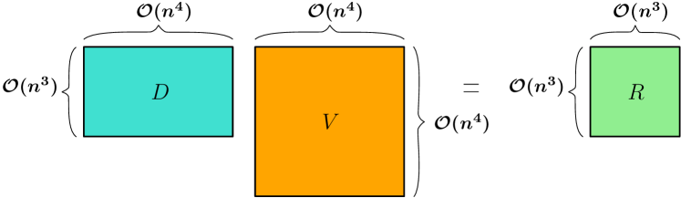
(a) Homology reduction

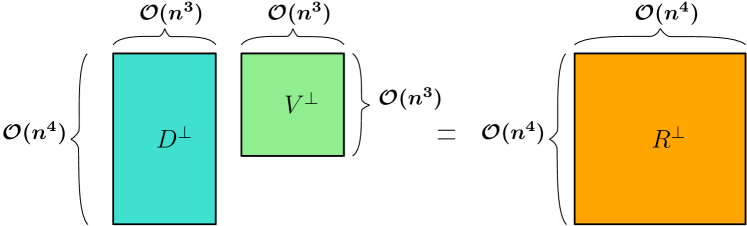
(b) Cohomology reduction

Figure 5: Matrix representation and bounds of PH computation for a data set with $n$ points.

3 Our Contribution

• A new way to index 2- and 3-simplices that significantly reduces memory requirement and also aids in reducing computation time.

• Algorithms to compute coboundaries for edges and triangles using our indexing method that optimize computation time of coboundary traversal during reduction.

• A fast implicit column algorithm to compute PH that can potentially reduce memory usage by a factor of the number of points in the data set without an inordinate increase in the computation time.

• Serial-parallel algorithm that distributes computation of PH over multiple threads without a significant increase in the total memory requirement.

• A computation of the PH of the human genome at high resolution, a data set with millions of points.

• Two versions of code—sparse and non-sparse. The sparse version requires memory proportional to the number of permissible edges in the filtration. The non-sparse version, while faster, requires memory proportional to the number of total edges possible in the data set.

4 Our Algorithm

The aim is to compute persistence pairs up to three dimensions for VR-filtration. We will refer to the 0-simplices as vertices ($v$), 1-simplices as edges ($e$), 2-simplices as triangles ($t$), and 3-simplices as tetrahedrons ($h$). Consider a point-cloud data set embedded in a metric space, that is, there is a well-defined distance metric between any two points (vertices) in the space. We denote the number of vertices by $n.$ The number of edges in the filtration, denoted by $n_{e},$ will depend upon the maximum permissible value of the filtration parameter, denoted by $\tau_{m}.$ If $\tau_{m}$ is small compared to the maximum distance in the data set, we expect $n_{e}\ll{n\choose 2}$ and we call the filtration sparse. Since the reduction operations are always between complexes of the same dimension, we construct VR-filtrations for each dimension separately. Let $\mathcal{S}^{d}$ be the set of all permissible simplices of dimension $d$ and $\mathcal{O}^{d}$ be the corresponding set of orders in the filtration. We define bijective maps $f_{d}:\mathcal{S}^{d}\to\mathcal{O}^{d}.$ Since all vertices are born at the same filtration parameter (zero), $f_{0}(v)$ for a vertex $v$ can be arbitrarily assigned a unique whole number. For convenience, we will use $f_{0}(v)$ and $v$ interchangeably. For edges, the map $f_{1}(e)$ is the indexing defined by the sorting algorithm applied to the lengths of the edges. The filtration for 0-simplices is then the list of vertices ordered according to $f_{0},$ and is denoted by $F_{0}.$ The filtration for 1-simplices is a list of edges ordered according to $f_{1},$ and is denoted by $F_{1}.$ Additionally, we will denote the list of $d$-simplices in the reverse order of filtration by $F^{-1}_{d}.$ To define filtrations for 2- and 3-simplices we introduce a new way to index triangles and tetrahedrons.

4.1 Paired-indexing and Neighborhoods

We first define the diameter of a simplex $\sigma$ in the filtration as the maximum of the orders of the edges in the simplex, denoted by $d(\sigma).$ The corresponding edge is denoted by $d^{-1}(\sigma).$ Then, paired-indexing uses a pair of keys, primary ($k^{p}$) and secondary ($k^{s}$), denoted by $\langle k^{p},k^{s}\rangle.$ The primary key for both triangles and tetrahedrons is their diameter and the secondary key is the order of the simplex defined by the remaining points. For a triangle $t=\{a,b,c\},$ if $d^{-1}(t)=\{a,b\},$ then $f_{2}(\{a,b,c\})=\langle f_{1}(\{a,b\}),f_{0}(\{c\})\rangle=\langle f_{1}(\{a,b\}),c\rangle.$ For a tetrahedron $h=\{a,b,c,d\},$ if $d^{-1}(h)=\{a,b\},$ then, $f_{3}(\{a,b,c,d\})=\langle f_{1}(\{a,b\}),f_{1}(\{c,d\})\rangle.$ We define an ordering on the paired-indexing as follows,

$$\langle k_{i}^{p},k_{i}^{s}\rangle>\langle k_{j}^{p},k_{j}^{s}\rangle\,\,\text{iff either}\,\,\{k_{i}^{p}>k_{j}^{p}\}\,\,\text{or}\,\,\{k_{i}^{p}=k_{j}^{p}\,\text{and}\,k_{i}^{s}>k_{j}^{s}\}.$$ (1)

This ordering on the paired-indexing preserves the order of the simplices in the VR-filtration since a simplex with the larger diameter will have a greater order in the filtration. Simplices with the same diameter can be ordered arbitrarily with respect to each other, which in paired-indexing is based on the secondary key. The maps $f_{2}$ and $f_{3}$ then define filtrations $F_{2}$ and $F_{3},$ respectively. We do not store these filtrations as lists in the algorithm and instead compute them on the fly, reducing the memory required. We say that a simplex in $\mathcal{S}^{d}$ is greater than another simplex in $\mathcal{S}^{d}$ iff its order in the filtration is greater.

The paired-indexing plays an important role in both reducing memory requirements and computation time. Using the 4 byte $\texttt{unsigned int},$ this indexing will take exactly 8 bytes to represent any triangle or tetrahedron in a filtration regardless of the number of points in the data set. Further, since $k^{p}$ and $k^{s}$ are less than $n_{e},$ the paired-indices are bounded by $\mathcal{O}(n_{e}),$ rather than $\mathcal{O}(n^{4}).$ This specifically reduces memory requirement by many orders of magnitude for sparse filtrations, where $n_{e}\ll{n\choose 2}.$

4.2 Computing Coboundaries

We show how paired-indexing can be used to compute coboundary of edges and triangles. We begin by defining vertex-neighborhood $(N^{a})$ and edge-neighborhood $(E^{a})$ of a vertex $a.$ The neighbor of the vertex $a$ is a vertex that shares an edge with $a.$ Both $N^{a}$ and $E^{a}$ are lists of all neighbors of $a.$ Each element of these lists is a structure that contains a neighbor of $a$ and the order of the edge between them. The vertex-neighborhood is sorted by the order of the neighbors and the edge-neighborhood is sorted by the order of the corresponding edges (see Figure 6). The vertex and edge neighborhoods of all vertices are computed using $F_{0}$ and $F_{1},$ and they are stored in the memory. We will use $F_{0}$ and $F_{1}$ in Figure 6 as an example to illustrate how paired-indexing can be used to compute coboundary of an edge and a triangle. For convenience, the order of an edge $\{a,b\},$ $f_{1}(\{a,b\}),$ is denoted by $ab.$

Figure 6: An example of a VR-filtration. $F_{0}$ is the list of vertices and $F_{1}$ is the list of edges, both sorted in the order of the filtration. The vertex- and edge-neighborhoods for vertex $a$ are shown as example. The dark border indicates that $N^{a}$ is sorted by the order of neighbors of $a$ and $E^{a}$ is sorted by the order of the corresponding edges.

4.2.1 Coboundaries of Edges

Consider the edge $\{a,b\}$ in Figure 6. Any simplex in its coboundary is a triangle $t=\{a,b,v\}=\left<k_{1},k_{2}\right>,$ where $v$ is a common neighbor of $a$ and $b$, and the diameter of $t=k_{1}\geq ab.$ We consider two cases: case 1, triangles with diameter equal to $ab,$ and case 2, triangles with diameter greater than $ab.$ The triangles in case 1 are smaller than those in case 2. Hence, to compute the simplices in the coboundary as ordered in $F_{2},$ we start in case 1—the primary key is $ab$ and the order of the simplices is decided by the vertex in $t$ that is not $a$ and $b,$ that is, $v.$ We traverse along the vertex-neighborhoods using indices $i_{a}$ and $i_{b}$ to find common neighbors in an increasing order. Initially, both are set to 0. As shown in Figure 7, we increment the index pointing to the lower ordered vertex till both indices point to the same vertex $v$, in which case, $v$ is a common neighbor and $\{a,b,v\}$ exists in the filtration. However, we have to ensure that its diameter is $ab$ since we are in case 1. For example, in (1) in Figure 7, we skip $\{a,b,d\}$ because $ad>ab$ (see $F_{1}$ in Figure 6). Note that the structures in vertex-neighborhoods give direct access to $av$ and $bv$ at $i_{a}$ and $i_{b}$ for comparison with $ab.$ Otherwise, if the diameter of $\{a,b,v\}=ab,$ then $\left<ab,v\right>$ is the next greater triangle in $\delta\{a,b\}$ in $F_{2}.$ This triangle is recorded as $\phi=(ab,i_{a},i_{b},\delta_{*})$ where $\delta_{*}=f_{2}(\{a,b,v\})=\left<ab,v\right>.$ We call this the $\phi$-representation of $\delta_{*}$ as a simplex in the coboundary of $\{a,b\}.$ If either of the indices reach the end of the corresponding neighborhood, we go to case 2.

In case 2, the triangles in $\delta\{a,b\}$ have diameter greater than $ab.$ Hence, their order in the filtration is defined by the diameter of the primary key. To compute the primary keys as ordered in $F_{2},$ we define $i_{a}$ and $i_{b}$ to be indices of the respective edge-neighborhoods since they are sorted by the order of the edges. We set $i_{a}$ and $i_{b}$ to point to the smallest edges greater than $ab$ (binary search operations in $E^{a}$ and $E^{b},$ respectively). We then consider the index that points to the lower ordered edge. For example, in (7) in Figure 7, $i_{a}=3$ points to $ad$ and $i_{b}=3$ points to $bg.$ We consider $i_{a}=3$ because $ad<bg.$ Now, we have to check that $\{a,b,d\}$ exists and its diameter is $ad.$ A single binary search operation over $N^{b}$ finds that $d$ is a neighbor of $b,$ confirming the existence of $\{a,b,d\},$ and it also gives us $bd.$ Since $ad<bd,$ the diameter of $\{a,b,d\}$ is not $ad$ and we do not record it as a coboundary. We proceed by incrementing $i_{a}$ by one. Now $i_{b}$ points to the smaller edge, and the corresponding triangle is $\{a,b,g\}.$ A binary search over $N^{b}$ finds that $g$ is not a neighbor of $a,$ hence, this triangle does not exist, and $i_{b}$ is incremented by 1 to continue. The index $i_{a}$ now points to the smaller edge ($af$), and the corresponding triangle is $\{a,b,f\}.$ Since, this triangle exists and $af$ is its diameter, $\left<af,b\right>$ is the next simplex in the coboundary and it is recorded as $\phi=(ab,i_{a},i_{b},\left<af,b\right>).$ This process is continued till both $i_{a}$ and $i_{b}$ reach the end of the respective edge-neighborhood.

The above computation yields the coboundary of $\{a,b\}$ as a list of tuples $\phi^{i}_{ab}$ (see Figure 7) in an increasing order. This is an inefficient method to compute the coboundary of a simplex if it needs to be computed only once. A faster method would be to create the entire list of simplices in the coboundary and sort it by the order. However, reduction can require the computation of the coboundary of a simplex multiple times. Further, it is not feasible to store the entire coboundary matrix a priori due to memory limitations—even the size of the coboundary of one simplex can be up to $O(n^{4})$(see Figure 5). Using our $\phi$-representation, we implement three algorithms to address both these issues. First, the smallest simplex in the coboundary of $\{a,b\}$ can be found simply by starting in case 1 with $i_{a}$ and $i_{b}$ initialized to 0, and we proceed as outlined previously. The first valid simplex encountered is the answer. This is implemented as FindSmallestt (algorithm 8). Second, given a tuple $\phi=(ab,i_{a},i_{b},\left<k_{1},k_{2}\right>),$ the next greater simplex in $\delta\{a,b\}$ can be computed as follows. If $k_{1}=ab,$ then $i_{a}$ and $i_{b}$ are indices of the vertex-neighborhoods (case 1) and if $k_{1}>ab,$ they are indices of edge-neighborhoods (case 2). After determining the scenario, we proceed as outlined previously. As a result, given the $\phi$-representation of a triangle $t$ in the coboundary of an edge $\{a,b\},$ we can compute the next greater triangle in its coboundary without always having to traverse entire neighborhoods of $a$ and $b.$ We implement this as FindNextt (algorithm 9). Third, given a triangle $\delta_{\#}=\left<k_{1},k_{2}\right>,$ the smallest simplex greater than or equal to $\delta_{\#}$ in the coboundary of an edge $\{a,b\}$ can be computed by considering three scenarios. (1) If $k_{1}<ab,$ then the triangle with the least order in the coboundary of $\{a,b\}$ is the answer. (2) If $k_{1}=ab,$ then we start in case 1 at indices $i_{a}$ and $i_{b}$ of vertex-neighborhoods that point to the neighbor with smallest order greater than or equal to $k_{2}$. If no such neighbor exists, then we initialize $i_{a}$ and $i_{b}$ to the beginning of case 2. (3) If $k_{1}>ab,$ then we start in case 2 at the indices $i_{a}$ and $i_{b}$ of edge-neighborhoods that point to the edges with smallest order greater than or equal to $k_{1}.$ This is implemented as FindGEQt (algorithm 10). Note that the search operations in all of these algorithms are binary search operations since vertex- and edge-neighborhoods are sorted. We will show in 4.3.2 how these three algorithms are utilized to reduce the coboundaries to compute persistence pairs. See appendix B for all pseudocode related to coboundaries of edges.

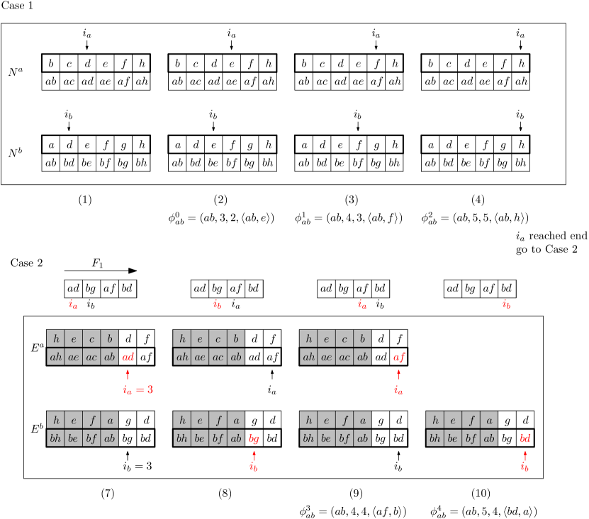
Figure 7: Using vertex- and edge-neighborhoods to compute simplices in the coboundary of edge $\{a,b\}$ (see Figure 6 for $F_{1}$), such that they are in the order of $F_{2}.$ The valid triangles are stored using $\phi$-representation.

4.2.2 Coboundaries of Triangles

Consider the triangle $t=\{a,b,e\}=\left<ab,e\right>$ in Figure 6. Any simplex in its coboundary is a tetrahedron $t=\{a,b,e,v\}=\left<k_{1},k_{2}\right>,$ where $v$ is a common neighbor of $a,b,$ and $e$, and the diameter of $h=k_{1}\geq ab.$ We will use three indices, $i_{a},i_{b},$ and $i_{e},$ to keep track of neighborhoods of $a,b,$ and $e,$ respectively. We consider two cases: case 1, tetrahedrons with diameter equal to $ab,$ and case 2, tetrahedrons with diameter greater than $ab.$ The tetrahedrons in case 1 are smaller than the triangles in case 2, so we start with case 1—the primary key is $ab$ and the order of the simplices is decided by the order of the edge $\{e,v\}.$ To compute such edges according to their order in $F_{1},$ we traverse through the edge-neighborhood of $e.$ Initially, $i_{e}$ is set to 0. For every edge $\{e,v\}$ that $i_{e}$ points to, we check whether $v$ is a neighbor of $a$ and $b$ to confirm existence of $\{a,b,e,v\},$ and we check that $ab$ is its diameter. These checks require two binary search operations, one each for $N_{a}$ and $N_{b}.$ If both conditions are satisfied, then we record the tetrahedron. We proceed by incrementing $i_{e}$ by one. For example, when $i_{e}=0$ in (1) in Figure 8, the resulting tetrahedron exists but $ab$ is not its diameter, and we do not record it. We skip when $i_{e}$ points to $ae$ or $be$ because they are not valid tetrahedrons. The first tetrahedron with diameter $ab$ is when $i_{e}=3,$ and hence, $\{a,b,e,h\}$ is the smallest tetrahedron in $\delta t.$ We define the $\phi$-representation for tetrahedrons as the tuple $\phi=(t,i_{a},i_{b},i_{e},f,\left<ab,eh\right>),$ where $f$ flags the diameter as follows—$f$ is $0,1,2,3$, and 4 correspond to diameter being $ab$, $ah$, $bh$, and $eh$, respectively. This flag is implemented to determine which index has to be incremented to find the next greater tetrahedron in $\delta t.$ For example, if $ab$ is the diameter, that is, $f=0,$ we are in case 1 and $i_{e}$ is to be incremented by one to proceed. Note that, in general, for any given triangle $t=\left<k^{p},k^{s}\right>,$ we compute $a\leftarrow\text{min}\{f^{-1}_{1}(k^{p})\},$ $b\leftarrow\text{max}\{f^{-1}_{1}(k^{p})\},$ and $e\leftarrow k^{s}.$ Case 1 is continued till $i_{e}$ points to an edge greater than $ab,$ since all tetrahedrons henceforth will have a diameter greater than $ab.$ In Figure 6, $ef>ab$ (indicated by a dashed line), hence we start with case 2 when $i_{e}=3.$

All valid tetrahedrons in case 2 that are in $\delta t$ will have diameter greater than $ab.$ The index $i_{e}$ already points to the entry in $E^{e}$ that has the smallest edge greater than $ab$. We implement binary search to compute $i_{a}$ and $i_{b}$ such that they also point to the smallest edge greater than $ab$ in the respective edge-neighborhood. All tetrahedrons in case 2 will have different primary keys since they have different diameters. Among the indices $i_{a},i_{b},$ and $i_{e},$ we consider the index that is pointing to the edge with the minimum order. As before, we have to check the existence of the tetrahedron and that its diameter is the edge under consideration. For example, in Figure 8, we begin case 2 in (5) by considering $i_{a}$ because it points to $ad=\text{min}\{ad,bg,ef\}.$ Binary searches for vertex $d$ over $N^{b}$ and $N^{e}$ confirm the existence of the tetrahedron $\{a,b,e,d\}$ and also show that $ad$ is not its diameter. Hence, this tetrahedron is not recorded and $i_{a}$ is incremented by 1 to proceed. Now, $i_{b}$ points to the smallest edge, but the resulting tetrahedron does not exist since $g$ is not a neighbor of $e.$ The smallest tetrahedron in case 2 is $\{a,b,e,d\},$ recorded at (8) as $(\left<ab,e\right>,6,5,4,2,\left<bd,ac\right>).$ Note that $f$ is 2 since the diameter is $bd.$ This flag dictates that $i_{b}$ is to be incremented by 1 to proceed because the current pointer being considered is $i_{b}.$ Similarly, if $f=1$ then $ad$ is the diameter and $i_{a}$ has to be incremented to proceed and if $f=3,$ then $ed$ is the diameter and $i_{e}$ has to be incremented by 1. The index $i_{e}$ is incremented to proceed when either $f=0$ or $f=3,$ but we are in case 1 in the former and in case 2 in the latter. Case 2 ends when all three indices reach the end of their respective edge-neighborhood.

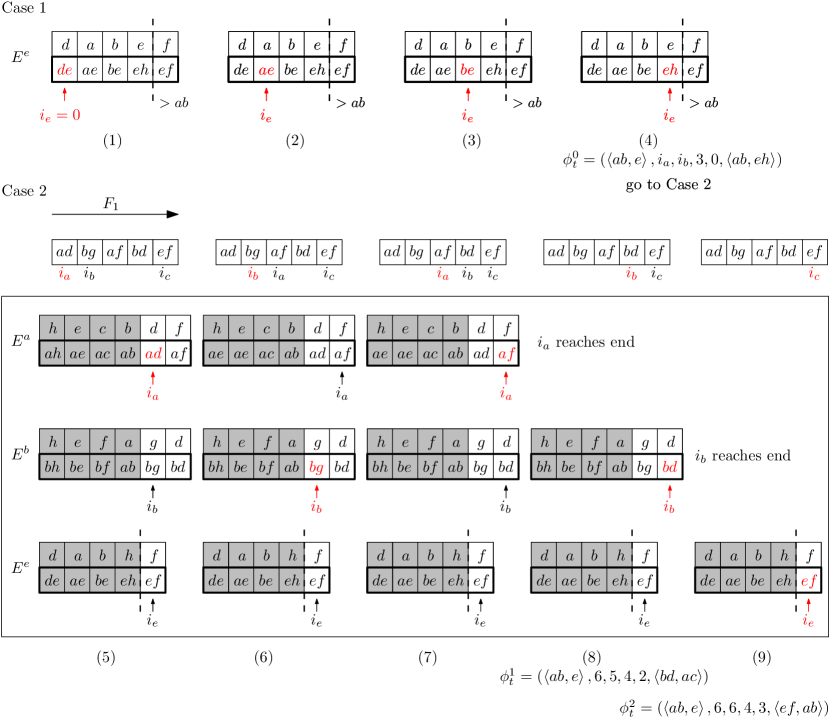
Figure 8: Using edge-neighborhoods to compute simplices in the coboundary of triangle $\{a,b,e\}$ (see Figure 6 for $F_{1}$), such that they are in the order of $F_{3}.$ The index marked in red in every iteration, points to the edge under consideration. The valid tetrahedrons are stored using $\phi$-representation.

The above computation yields the coboundary of $t=\{a,b,e\}$ as a list of tuples $\phi^{i}_{t}$ (see Figure 8). The case and the index to be incremented is determined by the flag $f$ as discussed previously. As done for edges, this $\phi$-representation is used to implement three algorithms—FindSmallesth, FindNexth, and FindGEQh. The smallest simplex in the coboundary of $t$ can be found simply by starting in case 1, initializing $i_{e}$ to 0, and proceeding as outlined previously. The first valid simplex encountered is the answer (algorithm 13). For FindNexth (algorithm 14), given the $\phi$-representation of a simplex $\left<k_{1},k_{2}\right>$ in $\delta t$ as $\phi=(t,i_{a},i_{b},i_{e},f,\left<k_{1},k_{2}\right>),$ the smallest simplex greater than $\left<k_{1},k_{2}\right>$ in $\delta t$ can be computed by proceeding in case 1 if $f=0$ and proceeding in case 2 otherwise—incrementing the indices by one as dictated by the value of $f.$ Finally, given a tetrahedron $\delta_{\#}=\left<k_{1},k_{2}\right>,$ the search for the smallest simplex greater than or equal to $\delta_{\#}$ in $\delta t$ is optimized by considering three scenarios (algorithm 15). (1) If $k_{1}<ab,$ then the smallest tetrahedron in $\delta t$ (FindSmallesth) is the answer. (2) If $k_{1}=ab,$ then we start in case 1 and search for $i_{e}$ that points to the smallest edge greater than or equal to $k_{2}.$ If no such edge exists, then we start in case 2 with $i_{e}$ pointing to the end of $E^{e}.$ (3) If $k_{1}>ab,$ we are in case 2 and we find the indices that are greater than or equal to $k_{1}$ in the respective edge-neighborhoods. See appendix C for all the pseudocode related to coboundaries of triangles.

4.3 Cohomology Reduction

To compute persistence pairs using cohomology reduction, we reduce one simplex at a time since it is often not feasible to store the coboundary matrix $D^{\bot}.$ Suppose the reduced coboundaries are stored in $R^{\bot}$ and the reduction operations are stored in $V^{\bot}.$ We will denote the column in $R^{\bot}$ that contains the reduced coboundary of edge $e$ by $R^{\bot}(e)$ and the corresponding column in $V^{\bot}$ by $V^{\bot}(e).$ Using this notation, the column reduction to reduce coboundary of one edge at a time is shown in algorithm 1. Here, low$(R^{\bot}(e))$ is the simplex with the smallest order in column $R^{\bot}(e).$ The partial reduction of the edge is stored in $r$ which initially is the coboundary of the edge. If low$(r)=$ low$(R^{\bot}(e^{\prime}))$ for some edge $e^{\prime},$ then $r$ is reduced (sum modulo 2) with $R^{\bot}(e^{\prime}).$ If no such edge exists or if $r$ is $\mathbf{0},$ then $r$ is completely reduced. A non-empty completely reduced $r$ is recorded as the column $R^{\bot}(e)$ or $R^{\bot},$ and (low($R^{\bot}(e)$), $e$) is a persistence pair.

1:Input: $F_{1}$

2:$R^{\bot}$ is empty

3:for $e$ in order of $F_{1}^{-1}$ do

4:     $r\leftarrow\delta e$

5:     while $r$ not empty AND there exists edge $e^{\prime}$ s.t. low$(R^{\bot}(e^{\prime}))=$ low$(r)$ do

6:         $r\leftarrow r\oplus R^{\bot}(e^{\prime})$      

7:     if $r$ not empty then

8:         $R^{\bot}(e)\leftarrow r$      

Algorithm 1 Starting with standard column reduction

4.3.1 Improving Scalability of Memory Requirement

However, Figure 5(b) shows that $R^{\bot}$ has the worst bounds on size. Therefore, we store only the reduction operations, that is, $V^{\bot}.$ Then, $r$ can be implicitly reduced with $R^{\bot}(e^{\prime})$ by summing (modulo 2) it with the coboundaries of edges in $V^{\bot}(e^{\prime})$ (see algorithm 2). This algorithm is implemented in Ripser. The smallest simplex $t$ after reducing coboundary of an edge $e^{\prime}$ is stored as a persistence pair $(t,e^{\prime})$ in $p^{\bot}.$ In this algorithm, the partial reduction operations are recorded in $v,$ the result of the ongoing reduction is in $r,$ and the smallest simplex in $r$ is stored as $\delta_{*}.$ However, keeping track of $r$ can require a lot of computer memory as its length is bounded by $O(n^{3})$ (and by $O(n^{4})$ when reducing triangles). We begin by proposing an implicit row algorithm that does not store $r$ at any stage of reduction, and it implicitly reduces $r$ using $v.$ Hence, its memory requirement depends on the size of $v$—$O(n^{2})$ for reducing edges and $O(n^{3})$ for reducing triangles, potentially reducing the memory requirement by a factor of $n.$

1:Input: $F_{1}$

2:$V^{\bot},p^{\bot}$ are empty

3:for $e$ in $F_{1}^{-1}$ do

4:     $r\leftarrow\delta e$

5:     $\delta_{*}\leftarrow$ low$(r)$

6:     $v\leftarrow[e]$

7:     while $\delta_{*}$ is not empty AND there is a pair $(\delta_{*},e^{\prime})$ in $p^{\bot}$ do

8:         for $e^{\prime\prime}$ in $V^{\bot}(e^{\prime})$ do

9:              $r\leftarrow r\oplus\delta e^{\prime\prime}$          

10:         $\delta_{*}\leftarrow\text{low}(r)$$\triangleright$ Update the low

11:         $v\leftarrow v\oplus V^{\bot}(e^{\prime})$$\triangleright$ Update reduction operations for $e$      

12:     if $\delta_{*}$ not empty then

13:         $V^{\bot}(e)\leftarrow v$

14:         $p^{\bot}\leftarrow(\delta_{*},e)$      

Algorithm 2 Do not store $R^{\bot}$: Implicitly compute from $V^{\bot}$

4.3.2 Implicit Row Algorithm

The reduction of the coboundary of an edge requires the computation of the smallest triangle in $r$ with non-zero coefficient, denoted by $\delta_{*}$ in the algorithm. Implicitly, $\delta_{*}$ is the smallest triangle with non-zero coefficient after coboundaries of all edges in the corresponding $v$ are summed. The idea behind the algorithm is that we will store $\phi$-representations of only the smallest triangle with non-zero coefficient in the coboundary of every edge in $v$, the function FindGEQt will optimize reduction by eliminating certain redundant reductions, and the function FindNextt will traverse along the coboundaries during reduction. We begin with introducing a basic strategy to compute $\delta_{*}$ in this algorithm. To explain the algorithm, we will walk through an example that reduces $r=\delta e_{0}$ with $R^{\bot}$ using only $v,$ $V^{\bot},$ and $p^{\bot}.$

Step 1 (‘initialize’ in Figure 9): As shown in the figure, $\delta^{0}$ is the smallest simplex in $\delta e_{0}.$ Then, $v$ is initialized as a list with the single entry of $\phi$-representation of $\delta^{0}$ in $\delta e_{0},$ denoted by $\phi_{e_{0}}=(e_{0},i_{a},i_{b},\delta^{0}).$ This corresponds to the information that $r=\delta e_{0}$ initially and the smallest triangle in $r$ is $\delta^{0}.$ Subsequently, $\delta_{*}$ is initialized with $\delta^{0}.$

Step 2 (‘append’ in Figure 9): Now, suppose there exists a pair $(\delta_{*},e^{\prime})$ in $p^{\bot}$ and $V^{\bot}(e^{\prime}_{0})=[e_{1}^{\prime},e_{2}^{\prime},e^{\prime}_{3}].$ Then, $r$ is to be summed with $R^{\bot}(e^{\prime}).$ Since the smallest triangle with non-zero coefficient in $R^{\bot}(e^{\prime})$ is $\delta_{*},$ we know that when coboundaries of all $e^{\prime}_{k}$ in $V^{\bot}(e^{\prime})$ are summed with each other, then every triangle that is smaller than $\delta_{*}$ will have a zero coefficient (shown as shaded area in the figure). Hence, triangles in $\delta e^{\prime}_{k}$ that are smaller than $\delta_{*}$ will have zero coefficient and they do not matter. Therefore, for every edge $e^{\prime}_{k}$ in $V^{\bot}(e^{\prime}_{0})$ and the edge $e^{\prime}_{0},$ we use FindGEQt to compute the smallest triangle in their coboundary that is greater than or equal to $\delta_{*},$ and append its $\phi$-representation to $v$ (see (0) in Figure 9). This eliminates unnecessary reductions of the coboundaries of the new edges that are being appended to $v.$ Moreover, FindGEQt does so efficiently by considering three cases and conducting binary searches as explained in 4.2.1. Hence, paired-indexing not only improves the limits on memory requirements, but also plays a crucial role in reducing the computation time of the reduction. The updated $v$ corresponds to the updated $r\leftarrow r\oplus R^{\bot}(e^{\prime}),$ therefore the coefficient of $\delta_{*}$ will be 0. To find the smallest triangle with non-zero coefficient in $r,$ we go to step 3.

Step 3 (‘reduce’ in Figure 9): We first define $\delta=\text{MAX}=\left<n_{e},0\right>$ (since $k_{1}<n_{e}$), and then we process every $\phi_{e}=(e,i_{a},i_{b},\delta_{e})$ in $v$ as follows. If $\delta_{e}=\delta_{*},$ then we find the next simplex greater than $\delta_{e}$ in coboundary of $e$ using FindNextt since the coefficient of $\delta_{*}$ is 0. If the updated $\delta_{e}$ is less than $\delta,$ then we set $\delta\leftarrow\delta_{e}$ and set the coefficient to 1, otherwise, 1 is added (modulo 2) to the coefficient. As a result, $\delta$ stores the smallest triangle greater than $\delta_{*}$ in $r,$ and we also keep track of its coefficient. For example, starting at (0) in Figure 9, $\delta_{e}=\delta_{1}$ for the edges $e^{\prime}_{3},e^{\prime}_{2},e^{\prime}_{1},$ and $e_{0}.$ For these edges we compute the next greater triangle in their respective coboundary using FindNextt. After iterating through all entries in $v,$ it is determined that $\delta^{1}$ is the smallest simplex greater than $\delta_{*},$ and it has a coefficient of 0 (see (1) in figure). We update $\delta_{*}\leftarrow\delta^{1}$ and $\delta\leftarrow$ MAX, and we iterate through all entries in $v$ as done previously. In (3) we get $\delta_{*}=\delta^{2}$ with non-zero coefficient. This signals the end of implicit reduction of $r$ with $R^{\bot}(e^{\prime}_{0}).$ To determine whether $r$ is to be reduced with another column of $R^{\bot},$ we check if there exists a persistence pair $(\delta_{*},e^{\prime\prime})$ in $p^{\bot}$ and go back to step 2 to append $V^{\bot}(e^{\prime\prime})$ to $v.$ Otherwise, $r$ is completely reduced and we go to the next step to update $p^{\bot}$ and $V^{\bot}.$ In general, it is possible that $\delta_{*}$ is empty, in which case $r$ was reduced to $\mathbf{0}$ and reduction ends without requiring any update to $p^{\bot}$ and $V^{\bot}.$

Step 4 (‘update’ in Figure 9): If $\delta_{*}$ is not empty, then we add the persistence pair $(\delta_{*},e_{0})$ to $p^{\bot}.$ To update $V^{\bot},$ we first sum all $\phi_{e}$ modulo 2. This is because a $\phi_{e}$ with zero coefficient implies that the entire coboundary of $e$ will sum to 0 when coboundaries of all edges in $v$ are summed. For every $\phi_{e}$ with non-zero coefficient, except for $\phi_{e_{0}},$ we append $e$ to the column $V^{\bot}(e_{0}).$ The edge $e_{0}$ is not appended to $V^{\bot}(e_{0})$ because $\phi_{e_{0}}$ will always have a coefficient 1 and we already store $e_{0}$ in the persistence pair $(\delta_{*},e_{0}).$ If the resulting $V^{\bot}(e_{0})$ is empty, then we do not make any record of it. This concludes the complete reduction of $r$ with $R^{\bot}.$

There are two pitfalls in the above strategy. First, if an edge $e_{i}$ occurs an even number of times in $v$ (has zero coefficient in $v$), then we know that its coboundary will sum to 0 after complete reduction of $r,$ and hence, calling FindNextt for each of the multiple entries of $e_{i}$ during reduction is redundant. The above algorithm trades the cost of computation of coefficient of edges in $v$ with the cost of computing coboundaries. This might be inefficient if there are many edges that sum to 0 in $v.$ Second, computation of $\delta_{*}$ requires traversal across all entries of $v$ at every step of reduction. This does not scale well if $r$ requires a lot of reductions and the corresponding $v$ has a large number of edges. We show next that both of these can be addressed simultaneously when iterating over $v$ during reduction if we ensure that $\phi$-representations in $v$ are always ordered appropriately. Further, we will use paired-indexing to optimize it, making it an efficient strategy in terms of both memory requirement and computation time taken.

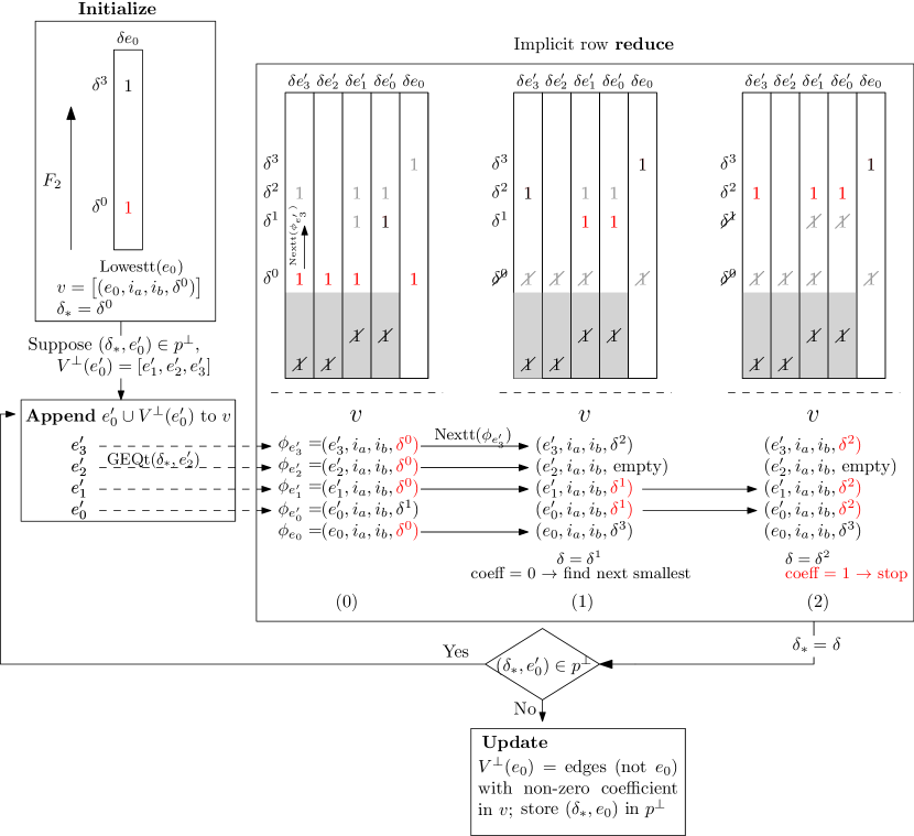
Figure 9: Example to show implicit reduction of $r=\delta e_{0}$ with $R^{\bot}$ using $V^{\bot}$ and $p^{\bot}.$ For every edge in $v,$ we record the smallest triangle in its coboundary with non-zero coefficient using the $\phi$-representation (marked in black). The smallest among these are marked in red. Simplices with zero coefficient are shown as crossed out.

4.3.3 Implicit Column Algorithm

Alternatively, we can view the $\phi$-representations in $v$ as a column of entries ordered first by the lows ($\delta_{i}$) and by the edges ($e_{i}$) for the same lows (see Figure 10). We say that $v$ is ordered by (low, edge). Then, entries in $v$ that correspond to the same lows or that correspond to the same lows in the coboundaries of the same edges, are adjacent to each other. As we move along $v,$ we sum adjacent entries and update the coefficient accordingly. For every $\phi_{i}$ in $v,$ we define a flag-next, denoted by $f^{i}_{n},$ that is flagged if the next triangle in the coboundary of the corresponding edge has to be computed and inserted in $v.$ We explain the algorithm below that can addresses the two pitfalls of implicit row algorithm. The flowchart is shown in Figure 10.

The first two steps of ‘initialize’ and ‘append’ are similar to 4.3.2 with two distinctions—new entries are inserted in $v$ such that it is ordered by (low, edge) and the flag-next of every new entry is initialized with 1. To reduce $v,$ we move along it linearly using a pointer, shown in red in Figure 10. It is initialized to point to the first index of $v.$ The only entry in $v$ initially is $(e_{0},i_{a},i_{b},\delta_{0}),$ hence, coeff is initialized to 1 and $\delta_{*}=\delta_{0}.$ Suppose we point at index $i$ of $v$ at the beginning of a reduction step. The coeff then has the coefficient of the entry at index $i.$ To compute $\delta_{*}$ (as defined in implicit row algorithm), we compare the adjacent entries in $v$ and update the coefficient. If $\delta_{i}=\delta_{i+1},$ then the coefficient is summed by 1 (modulo 2). Additionally, if $e_{i}$ is also equal to $e_{i+1},$ we unflag $f^{i}_{n}$ and $f^{i+1}_{n}$ if both are flagged. This eliminates edges $e_{i}$ and $e_{i+1}$ from subsequent computation of $\delta_{*},$ which is justified since coboundaries of equal edges will always sum to 0—resolving the first pitfall discussed in 4.3.2. Now, if $f^{i}_{n}$ is flagged, we compute $\phi^{\prime}_{i}=$ FindNextt$(\phi_{i})$, unflag $f^{i}_{n}$, and insert $\phi^{\prime}_{i}$ in $v.$ It is known that the index of $\phi^{\prime}_{i}$ in $v$ will be strictly greater than $i$ since it has a greater low than $\phi_{i}.$ So, the insertion of an element in $v$ does not affect $v$ up to and including index $i,$ and we can by incrementing $i$ by 1. Otherwise, if $\delta_{i}\neq\delta_{i+1},$ we look at the coefficient. If coeff $=1,$ then $\delta_{i}$ has non-zero coefficient and, hence, $\delta_{*}=\delta_{i},$ and we are done with reduction. On the other hand, the value 0 of coeff implies that $\delta_{i}$ has 0 coefficient. To proceed, we insert FindNextt$(\phi_{i})$ in $v$ if $f^{i}_{n}$ is flagged, and we unflag $f^{i}_{n}.$ Additionally, we reset coeff to 1 to indicate that the smallest triangle with non-zero coefficient is now $\delta_{i+1}.$ Then, we increment $i$ by one to continue computation of $\delta_{*}.$ A value of 0 for the coefficient of the last entry in $v$ implies that $r$ is reduced to $\mathbf{0}.$

In implicit row algorithm, it was a requirement to traverse through entire $v$ every time the coefficient of $\delta_{*}$ is 0. In implicit column algorithm also we have to traverse through $v$ to maintain the order of the entries, but this traversal is not necessarily across all $v.$ This potential improvement in computational efficiency is then canceled by the fact that the traversal in implicit column algorithm has to be done every time FindNextt is called and a new entry is inserted in $v.$ Further, since we insert entries in $v$ in implicit column algorithm in contrast to replacing them in implicit row algorithm, the size of the data structure that stores $v$ is theoretically bounded by the size of $r.$ As a result, this algorithm is not practically feasible yet, and in the next section we will show next how paired-indexing will solve both of these issues.

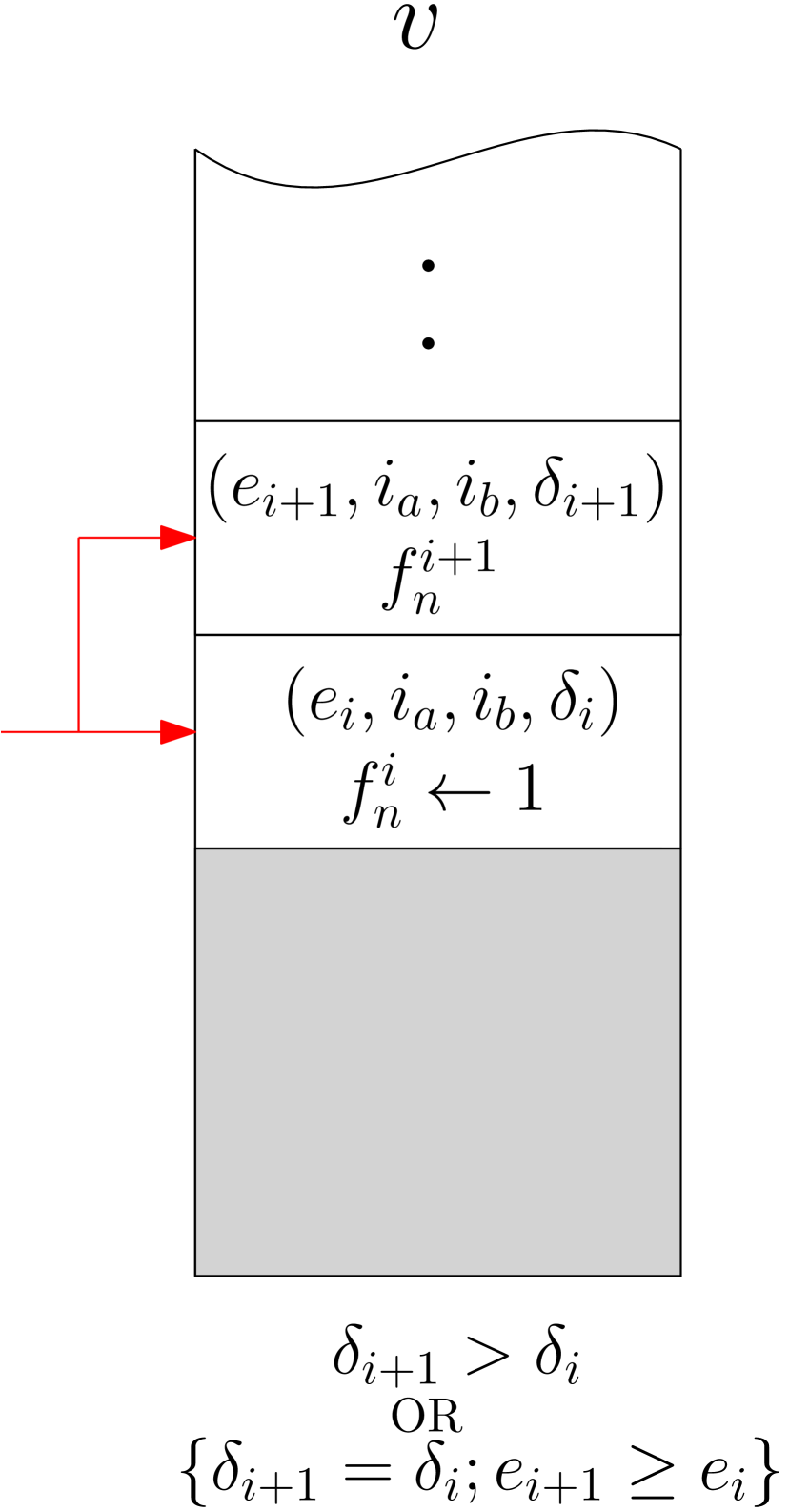
(a) New entries are now inserted in $v$ such that order is maintained as shown by the rule in the figure.

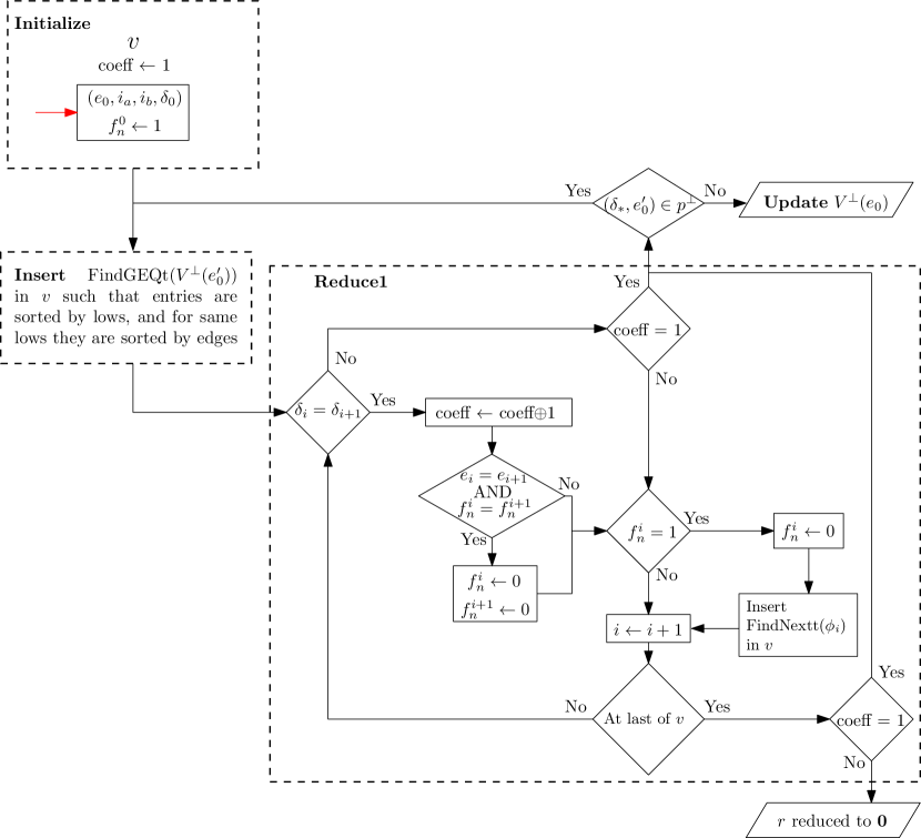
(b) Flowchart to compute $\delta_{*}$ with non-zero coefficient.

Figure 10: Implicit column algorithm.

4.3.4 Fast Implicit Column Algorithm

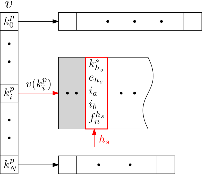
(a) $v$ is stored as a hash table with the primary keys of lows as its keys. The two red arrows collectively point to $\phi=(e_{h_{s}},i_{a},i_{b},\left<k^{p}_{i},k^{s}_{h_{s}}\right>)$

.

(b) Flowchart for inserting new entries in the hash table of $v.$

Figure 11: Fast implicit column algorithm, using paired-indexing to make a hash table.

To efficiently compute $\delta_{*}=\left<k^{p}_{*},k^{s}_{*}\right>,$ the smallest triangle with non-zero coefficient, we first observe that it will have the smallest primary key among all lows in $v.$ Now, using paired-indexing, we can store $v$ as a hash table that is defined by a list of unique primary keys that are in the lows of the entries in $v,$ and each entry in this list is mapped to a list of lows in $v$ that have the same primary key. Figure 11(a) shows an example of such a hash map. The keys of this hash table are stored as a linear list of primary keys $[k^{p}_{i}]$ (in no particular order), and each primary key is mapped to a linear list $v(k^{p}_{*}),$ with elements of the form $(k^{s},e,i_{a},i_{b},f_{n}).$ In Figure 11(a), the entry in the red box is at index $h_{s}$ of $v(k^{p}_{i})$, and it corresponds to $\phi=(e_{h_{s}},i_{a},i_{b},\left<k^{p}_{i},k_{h_{s}}^{s}\right>)$ with the corresponding flag-next $f^{h_{s}}_{n}.$

To compute $\delta_{*}$ using this hash table, we first find the primary key with the smallest order, denoted by $k^{p}_{*},$ and then compare adjacent entries in $v(k^{p}_{*})$ (see flowchart in Figure 12). That is why, the entries in $v(k^{p}_{*})$ have to be ordered by secondary key and those with same secondary key have to be ordered by the edge. We denote this ordering by (secondary key, edge). Note that, the order of elements of $v(k^{p})$ for $k^{p}\neq k^{p}_{*}$ does not matter. To ensure this, we define the insertion of a new entry in this hash table as follows (see Figure 11(b)). Suppose the new entry to be inserted is $\left(e,i_{a},i_{b},\left<k^{p},k^{s}\right>\right).$ If $k^{p}=k^{p}_{*},$ then $(k^{s},i_{a},i_{b},f_{n}=1)$ is inserted in $v(k^{p}_{*})$ such that its entries are ordered according to (secondary key, edge). Otherwise, we check whether $k^{p}$ exists in the list of keys of the hash table. If true, we append $(k^{s},i_{a},i_{b},1)$ to the end of $v(k^{p})$ since the order of its entries does not matter. If $v(k^{p})$ does not exist, then we append $k^{p}$ to the list of keys of the hash table, and we map $v(k^{p})$ to a list with a singular entry of $(k^{s},i_{a},i_{b},1).$ In this strategy, it is not required for entries in $v(k^{p})$ to be in a specific order when $k^{p}\neq k^{p}_{*},$ and we also do not maintain the order of the list of keys of the hash table. Hence, we maintain the order only of the entries that are crucial for computation of $\delta_{*},$ that is, precisely those that have the primary key as the smallest key of the hash table in the current reduction iteration. This optimizes the computational overhead of maintaining the order during insertion of new entries in $v.$

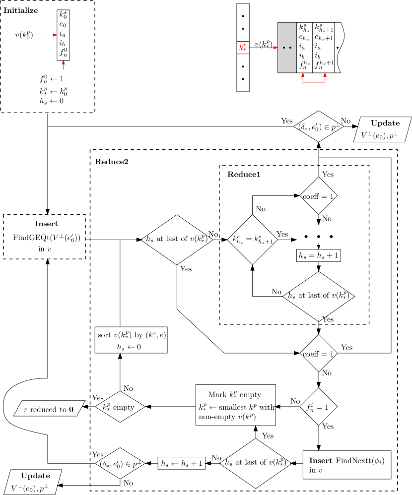
Figure 12: Flowchart for fast implicit column algorithm in which $v$ is stored as a hash table using paired-indexing. The three dots in box ‘Reduce1’ denote that it is similar to the flowchart in Figure 10(b).

Now, if $h_{s}$ reaches the last entry of $v(k^{p}_{*}),$ it does not imply that we have reached the last entry of the hash table, and we proceed as follows. If coeff$=1,$ then $\delta_{*}=\left<k^{p}_{*},k^{s}_{h_{s}}\right>$ and we are done. Otherwise, if coeff$=0,$ then we first check whether $f^{h_{s}}_{n}$ flagged. If it is flagged, we compute $\left(e_{h_{s}},i_{a},i_{b},\left<k^{p}_{\#},k^{s}_{\#}\right>\right)=$ FindNextt$\left(\left(e_{h_{s}},i_{a},i_{b},\left<k^{p}_{*},k^{s}_{h_{s}}\right>\right)\right)$ and insert it in the hash table. If $k^{p}_{\#}=k^{p}_{*},$ then $(k^{s}_{\#},e,i_{a},i_{b},1)$ is the last entry in the updated $v(k^{p}_{*}),$ and also, $h_{s}$ does not point to the last entry in $v(k^{p}_{*}).$ We know that the next simplex in $\delta e_{h_{s}}$ will be greater than $\left<k^{p}_{\#},k^{s}_{\#}\right>,$ hence, it is not required to compute FindNextt again, and $\left<k^{p}_{\#},k^{s}_{\#}\right>$ will have a coefficient of one. So, $\delta_{*}=\left<k^{p}_{*},k^{s}_{h_{s}+1}\right>=\left<k^{p}_{\#},k^{s}_{\#}\right>$ and we are done. Otherwise, if $k^{p}_{\#}\neq k^{p}_{*}$ or if $f^{h_{s}}_{n}$ was unflagged, we have traversed through all entries in $v(k^{p}_{*})$ and we mark the memory occupied by $v(k^{p}_{*})$ as free space that can be overwritten. As a result, the memory used by the hash table will never approach $r,$ addressing the second pitfall discussed in 4.3.3. To proceed, we iterate through rest of the keys of the hash table (that are not empty) and update $k^{p}_{*}$ with the smallest primary key. Since $v(k^{p}_{*})$ might not be sorted, we first sort it by (secondary key, edge). Then, we update $h_{s}\leftarrow 0$ and coeff$\leftarrow 1$, and we proceed with the computation of $\delta_{*}.$ If there are no keys left in the hash table, then $r$ was reduced to $\mathbf{0}.$

The fast implicit column algorithm to compute $H_{2}^{*}$ similarly uses paired-indexing along with the $\phi$-representation for tetrahedrons introduced in Section 4.2.2 and the functions FindSmallesth, FindNexth, and FindGEQh. It scales more efficiently than the implicit row algorithm. See 4 in appendix E for a comparison between the two algorithms for test data sets that are used for benchmarking in this study (Section 5).

4.3.5 Trivial Persistence Pairs

(a) If $\left<ab,c\right>$ is the smallest triangle in $\delta\{a,b\},$ then $(\left<ab,c\right>,ab)$ is a trivial persistence pair.

(b) If $\left<ab,d\right>$ is the greatest triangle in the boundary of $\left<ab,cd\right>,$ and if $\left<ab,cd\right>$ is the smallest tetrahedron in $\delta\{a,b,d\},$ then $(\left<ab,cd\right>,\left<ab,d\right>)$ is a trivial persistence pair.

Figure 13: Trivial persistence pairs

For further reduction in memory usage, we notice that there are specific persistence pairs that can be computed on the fly and do not require storage in $p^{\bot}.$ Figure 13 shows an example of coboundary matrices for edges and triangles. The triangle $t=\left<ab,c\right>$ will be in the coboundary of exactly three edges (see Figure 13(a)). Since the diameter of $t$ is $\{a,b\},$ the row of $t$ will have all zeroes to the left of $(\left<ab,c\right>,ab).$ If additionally, $t$ is the smallest simplex in the coboundary of $\{a,b\},$ then there will be all zeroes below $(\left<ab,c\right>,ab).$ Consequently, $(\left<ab,c\right>,ab)$ will be a persistence pair and will not require any reduction. We will call such pairs trivial persistence pairs, and we will not store them in $p^{\bot}.$ Instead, during the reduction of $r,$ we check whether $\delta_{*}=\left<k_{1},k_{2}\right>$ is the smallest simplex in the coboundary of the edge $e^{\prime}=f_{1}^{-1}(k_{1})$. If true, then $(\delta_{*},e^{\prime})$ is a trivial persistence pair and the next reduction is to be with exactly the coboundary of $e^{\prime}$ (since trivial persistence pairs do not require any reductions). Conducting this check at every step of reduction is computationally feasible because paired-indexing gives direct access to the diameter of $t,$ making these checks inexpensive. For further optimization, the smallest simplex in the coboundary of each edge is stored a priori at the cost of $O(n_{e})$ memory.

Similarly, a tetrahedron, $h=\left<ab,cd\right>,$ will be in the coboundary of exactly four triangles (see Figure 13(b)). The greatest triangle in the boundary of $h$ will be $t=\left<ab,\text{max}\{c,d\}\right>.$ Following similar reasoning, if $h$ is the smallest simplex in the coboundary of $t,$ then we say that $(h,t)$ is a trivial persistence pair. During reduction of any triangle, we check whether $\delta_{*}=\left<k_{1},k_{2}\right>$ is the smallest simplex in the coboundary of the triangle $t^{\prime}=\left<k_{1},\text{max}\{f_{1}^{-1}(k_{2})\}\right>$. If true, $(\delta_{*},t^{\prime})$ is a trivial persistence pair and the next reduction is to be with the coboundary of $t^{\prime}.$ FindSmallesth is used to check whether $\delta_{*}$ is the smallest simplex in $\delta t^{\prime}.$

4.4 Parallelizing: A General Serial-parallel Reduction Algorithm

To reduce the computation time required to process the large number of simplices in the VR-filtration, we developed a novel serial-parallel algorithm that can reduce multiple simplices in parallel. In essence, rather than reducing one simplex at a time, we will reduce a batch of simplices. Any algorithm cannot be embarrassingly parallel because of the inherent order in reduction imposed by the filtration. We introduce the serial-parallel algorithm by parallelizing the standard column algorithm (algorithm 1) for cohomology computation (see Figure 16).

Parallel (Figure 14(a)): Suppose $R^{\bot}$ contains reductions of the first $n$ edges in $F^{-1}.$ Let $\mathbf{r}=[r_{1},...,r_{B}]$ be the batch of next $B$ edges in $F_{1}^{-1}$ that have to be reduced. Initially, each $r_{i}$ is the coboundary of the corresponding edge, and during reduction it contains the result of the ongoing reduction. Then, if the low of $r_{i}$ and $r_{j}$ in $\mathbf{r}$ is equal to that of $R^{\bot}(e)$ for some edge $e,$ reducing $r_{i}$ and $r_{j}$ with $R^{\bot}(e)$ will take precedence over reducing them with each other. As a result, each $r_{i}$ can be reduced with $R^{\bot}$ in parallel.

(a) Parallel reduction: Each $r_{i}$ is reduced with $R^{\bot}$ independently, in parallel.

(b) Serial reduction: After parallel reduction, columns in $\mathbf{r}$ are reduced with each other.

Figure 14: Flowcharts for parallel and serial reductions that form the serial-parallel algorithm.

Serial (Figure 14(b)): After $\mathbf{r}$ has been reduced with $R^{\bot},$ we reduce the columns in $\mathbf{r}$ with each other using serial reduction. We ‘mark’ $r_{i}$ if it is completely reduced. After parallel reduction, none of the $r_{i}$ have the same low as any column in $R^{\bot}.$ Hence, $r_{1}$ is completely reduced and we mark it. Then, carrying out the standard column algorithm, the low of every $r_{i}$ ($i>1$) is compared sequentially with $r_{j}$ for every $j<i.$ We consider the following cases for every $r_{j}.$ (1) If low($r_{j}$) $>$ low($r_{i}$), then we skip it. (2) Otherwise, we check whether $r_{j}$ is marked. (2a) If it is unmarked, we cannot continue reduction of $r_{i}$ before reducing $r_{j}$ so we unmark $r_{i}$ and increment $i$ by one. (2b) If $r_{j}$ is marked and low($r_{j}$) $=$ low($r_{i}$), then we reduce $r_{i}$ with $r_{j},$ and we check whether the new low of $r_{i}$ is also the low of a column in $R^{\bot}.$ If true, then $r_{i}$ has to be reduced with $R^{\bot}$ before reducing with any $r_{j}$ in $\mathbf{r}$, and we unmark $r_{i}$ and increment $i$ by one. Otherwise, if the updated low is not the low of any column in $R^{\bot},$ then $j\to 1.$ This process is repeated to reduce $r_{i}$ until either $j$ reaches $i$ or $r_{i}$ is unmarked. When all of $\mathbf{r}$ has been processed, that is, $i$ reaches the end of $\mathbf{r},$ we go to clearance. A detailed hypothetical example is shown in Figure 15.

Clearance: All marked $r_{i}$ are appended to $R^{\bot},$ freeing up space in $\mathbf{r}$ to be filled in by the coboundaries of the next edges from $F_{1}^{-1}.$ After filling $\mathbf{r}$ with the new coboundaries, we go back to parallel reduction. This process is continued until all edges in $F_{1}^{-1}$ have been reduced. The structure of the algorithm is shown in Figure 16.

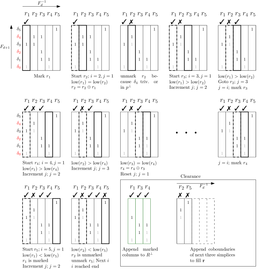
Figure 15: Hypothetical example to illustrate serial reduction in serial-parallel algorithm. The simplices marked by red indicate that they are in a persistence pair in $p^{\bot}.$

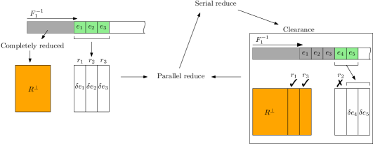
Figure 16: Serial-parallel algorithm to reduce coboundaries of edges. Similar algorithm structure is used to parallelize reduction of coboundaries of edges (H${}_{1}^{*}$) and triangles (H${}_{2}^{*}$) and to reduce boundaries of edges (H₀).

In Dory, we implement the serial-parallel algorithm to compute H${}_{0},$ H${}^{*}_{1},$ and H${}^{*}_{2}.$ We discuss the implementation for cohomology computation in detail. The batch to be reduced is represented by $\mathbf{v}=[v_{1},...,v_{B}],$ and we store $V^{\bot}$ and $p^{\bot}.$ Then, reducing $r_{i}$ with $R^{\bot}$ is implemented using the fast implicit column algorithm using $v_{i}$ and $V^{\bot},$ as shown earlier. The implicit reduction of $r_{i}$ with $r_{j}$ using $v_{i}$ and $v_{j}$ is modified slightly because $v_{j}$ stores the $\phi$-representations and FingGEQh is not required when appending $v_{j}$ to $v_{i}.$ Suppose $k^{p}_{j*}$ is the smallest primary key in $v_{j}$ and $h^{j}_{s}$ is the index in $v(k^{p}_{j})$ that points to the smallest low with non-zero coefficient. Then, merging $v_{i}$ with $v_{j}$ is done by inserting every entry of $v_{j}$ in $v_{i},$ except for the entries that are in $v(k^{p}_{j*})$ before the index $h^{j}_{s}.$ Additionally, trivial persistence pairs are not stored and are computed on the fly in the parallel reduction. The modified flowcharts are shown in Figure 17. For different scenarios during serial reduction, we use four different flags for every $r_{i}$—$f_{v}$ flags whether $r_{i}$ has to be reduced with a trivial persistence pair; $f_{r}$ flags whether $r_{i}$ is to be reduced with $R^{\bot}$; $f_{a}$ is flagged if it is completely reduced; and $f_{e}$ is flagged if $r_{e}$ is empty. Note that flagging $f_{v}$ and $f_{r}$ is similar to unmarking $r_{i},$ and flagging $f_{a}$ is similar to marking $r_{i}.$ The basic flow of the serial-parallel algorithm to reduce triangles is shown in algorithm 16. See appendix D for pseudocode of serial (algorithm 18) and parallel (algorithm 17) reduction. The default value of the batch-size for serial-parallel implementation of H${}^{*}_{2}$ computation is chosen as 100 and for H₀ it is 1000. These hyperparameters can be optimized for any data set. A smaller value of batch-size can increase the computation time by lowering the number of simplices that are reduced in parallel, but a larger value of batch-size can increase the computation time spent in the serial reduction. The parallelized section of the serial-parallel algorithm will be called many times in the serial-parallel reduction. To reduce the overhead of creating and destroying threads, we create threads before the computation of PH. The jobs are allocated in fixed chunks to these threads and the threads are woken up when they are required and destroyed after computaton of PH. We use light-weight POSIX threads, or pthreads.

(a) Implicit reduction of a single $r_{i}$ in the parallel reduction.

(b) Serial reduction.

Figure 17: Flowcharts for algorithms in serial-parallel reduction using fast implicit column algorithm and incorporating trivial persistence pair computation.

4.5 All Together with Clearing Strategy

We summarize the algorithm to compute the persistence pairs for groups H${}_{0},\text{H}^{*}_{1},$ and H${}^{*}_{2}$ in algorithm 3, including the clearing strategy suggested by Chen and Kerber (2011). This strategy provides significant reduction in computation time of cohomology reduction by eliminating the need for reduction of certain simplices. In essence, if $(\tau,\sigma)$ is a persistence pair in H_d (or $(\sigma,\tau)$ is in H${}^{*}_{d}$), then there cannot exist a persistence pair $(\sigma,\omega)$ in H${}_{d+1}.$ Consequently, there cannot exist a pair $(\omega,\sigma)$ in H${}^{*}_{d+1},$ and there is no need to reduce the coboundary of $\sigma$ when computing H${}^{*}_{d+1}.$

1:Input: $F_{1}$

2:Output: Persistence pairs in $\text{H}_{0},\text{H}^{*}_{1},\text{H}^{*}_{2}$

3:

4:for $e$ in $F_{1}$ do$\triangleright$ Compute H₀

5:     Serial-Parallel reduction

6:

7:for $e$ in $F^{-1}_{1}$ do$\triangleright$ Compute H${}^{*}_{1}$

8:     if $e$ is in a persistence pair in H₀ then$\triangleright$ Clearing strategy

9:         continue      

10:     Reduction

11:

12:for $e$ in $F^{-1}_{1}$ do$\triangleright$ Compute H${}^{*}_{2}$

13:     for $t$ in $\delta e$ with $d(t)=e$ do

14:         if $t$ is in a persistence pair in H${}^{*}_{1}$ then$\triangleright$ Clearing strategy

15:              continue          

16:         Serial-parallel reduction      

Algorithm 3 Computing all

4.6 Sparse vs. Non-Sparse

In the case of non-sparse filtrations, our experiments showed that most of the computation time was being spent on the binary searches in edge- and vertex-neighborhoods to find orders of the edges during cohomology computation. We implemented an alternate version in which we use combinatorial indexing to store the orders of all edges in the filtration. This reduces computation time by replacing binary search by an array access at the cost of using $O(n^{2})$ memory instead of $O(n^{2}_{e}).$ We call the non-sparse version DoryNS. In most cases it is advisable to use Dory because the reduction in peak memory usage outweighs the computation cost. DoryNS should be considered when computing H₂ for non-sparse filtrations.

5 Computation and Benchmarks

Data set	$n$	$\tau_{m}$	$n_{e}$	$d$	$N$
dragon	2000	$\infty$	1999000	1	1333335000
fractal	512	$\infty$	130816	2	2852247168
o3	8192	1	327614	2	33244954
torus4(1)	50000	0.15	2242206	1	41629821
torus4(2)	50000	0.15	2242206	2	454608895
Hi-C (control)	3087941	400	51233398	2	110946257
Hi-C (auxin)	3087941	400	35170863	2	36012219

Table 1: Data sets used for benchmarking in this study.

We tested Dory with six data sets—dragon, fractal, o3, torus4, Hi-C control, and Hi-C auxin (Table 1). The data sets dragon and fractal were used in Otter et al. (2017) to benchmark PH algorithms, o3 and torus4 are taken from the repository of Ripser (Bauer, 2019), and the Hi-C data sets are from Rao et al. (2017). They are briefly described as follows—dragon is a point-cloud in 3-dimensional space; fractal is the distance matrix for nodes in a self-similar network; o$3$ consists of 8192 random orthogonal $3\times 3$ matrices, that we consider as a point-cloud in nine dimensional space; torus4 is a point-cloud randomly sampled from the Clifford torus $S^{1}\times S^{1}\subset\mathbb{R}$; and the two Hi-C data sets are correlations matrices for around three million points (see Section 6 for more details). The benchmarks for PH computation of torus4 data set up to and including H${}^{*}_{1}$ are shown as torus4(1) and up to and including H${}^{*}_{2}$ are shown as torus4(2). The data sets can be found at https://github.com/nihcompmed/Dory. All computations are done on a computer with a 2.4 GHz 8-Core Intel Core i9 processor and 64 GB memory. We first comment on the computation time and memory taken by Dory.

Data set	Creating $F_{1}$	Creating $N^{v},E^{v}$	H0	H${}^{*}_{1}$	H${}^{*}_{2}$
dragon	1.14	0.488	0.144	0.36	NA
fractal	0.09	$\approx 0$	0.01	0.03	30.5
o3	0.4	0.03	0.03	1.4	2.9
torus4	5.74	0.66	0.25	1.95	30.68
Hi-C (control)	26.47	17.29	41.17	106.98	68.94
Hi-C (auxin)	17.64	10.29	21.57	20.35	15

Table 2: Time taken in seconds for different processes in Dory (4 threads and without -D PRINT compiler flag so that it does not print the persistence pairs in the terminal window).

The computation time taken by Dory can be split into following processes—create $F_{1},$ create the vertex- and edge-neighborhoods, and compute the persistence pairs (see Table 2 for results with Dory using 4 threads). In the dragon data set, almost half of the computation time is spent in creating $F_{1}.$ We believe that this can be significantly improved since we call a memory allocation for every edge in the current version of Dory. The other process in Table 2 that takes a significant amount of time is the computation of H${}^{*}_{2}.$ This follows from the facts that there are generally more simplices to be processed as compared to H${}^{*}_{1}$, and that all computations of coboundaries of triangles require binary searches, whereas, computation of coboundary of an edge does not require binary search when in Case 1 (Section 4.2.1). We improved the latter by implementing the non-sparse version, DoryNS at the cost of higher peak memory usage (see Table 3). The former might be improved by determining special classes of persistence pairs a priori (Bauer, 2019) that have been shown to not require any reductions, but their implementation and impact on computational feasibility within Dory’s framework is not yet clear and is an ongoing work.

The memory taken can be split into two parts—the base memory that is used by $F_{0},F_{1},$ and the vertex- and edge-neighborhoods, and the PH-memory used for homology and cohomology computations. The practical difference between these is that the base memory is known before computation of PH to be exactly $(3n+12n_{e})\times 4$ bytes in Dory for a data set with $n$ points and $n_{e}$ permissible edges in the filtration (see appendix E for this calculation), but PH-memory can be significantly more depending upon the reduction operations that need to be stored. Hence, the scaling of PH-memory can decide the feasibility of computation of PH for a data set.

Since Ripser outperforms both Gudhi and Eirene in computing PH for VR-filtrations, we compare time taken and peak memory usage between Dory and Ripser in this section (see Table 3), and the results with Gudhi and Eirene can be found in appendix E. The Ripser source file was downloaded from https://github.com/Ripser/ripser and compiled using c++ -std=c++11 ripser.cpp -o ripser -O3. DoryNS was compiled using the additional flag -D COMBIDX. Both were executed in the terminal of macOS (v 10.15.7). The computation time is the ‘total’ as reported by the command time and the peak memory usage was recorded using the application Instruments (v 12.2) in macOS in a separate execution.

Data set	Ripser	Dory		DoryNS
		4 thds.	1 thd.	4 thds.	1 thd.
dragon	(2.57 s, 199 MB)	(2.8 s, 262 MB )	(3.3 s, 270 MB )	(3.16 s, 277 MB)	(3.59 s, 269 MB)
fractal	(7.54 s, 775.13 MB)	(31.9 s, 695 MB)	(40.5 s, 687 MB)	(21.6 s, 810 MB)	(23.8 s, 802.8 MB)
o3	(6.47 s, 219 MB )	(5.07 s, 157 MB)	(6.43 s, 149 MB)	(4.86 s, 285 MB)	(6.2 s, 277 MB)
torus4(1)	(31.54 s, 12 GB )	(8.83 s, 328 MB)	(10.9 s, 321 MB)	(11.7 s, 5 GB )	(13.6 s, 5 GB)
torus4(2)	(94 s, 12 GB )	(40.74 s, 1 GB)	(59.3 s, 1 GB )	(42.7 s, 5.7 GB)	(60 s, 5.7 GB)
Hi-C (control)	NA	(276 s, 6.23 GB)	(540 s, 6.21 GB)	NA	NA
Hi-C (Auxin)	NA	(123 s, 3.98 GB )	(230 s, 3.98 GB )	NA	NA

Table 3: Time taken (seconds) was measured using the command time in the terminal of macOS. Peak memory usage is recorded using the application Instruments in macOS. The highlighted results indicate efficient performance.

We first address the benchmarks in Table 3 in which Ripser does better than Dory. For the dragon data set, Dory is slower than Ripser by $\approx 0.2$ s and takes $80$ MB more memory. The former can be attributed to the inefficiency of creating $F_{1}$ in Dory for which it takes almost half the total runtime for this data set. The higher peak memory usage can arguably be explained by the differences in the base memory because Dory additionally creates vertex- and edge-neighborhoods. However, as the size of the data set increases, the PH-memory will generally define the peak memory usage. For the fractal data set, Dory is slower than Ripser by a factor of 3 because Ripser identifies a large number of simplices that do not require any reduction during H${}^{*}_{2}$ computation of this data set. Implementation of this strategy in Dory is an ongoing work. DoryNS is faster than Dory, but it is still slower than Ripser for this data set. It is advisable to use Ripser to compute H${}^{*}_{2}$ for small data sets that are non-sparse.

For larger data sets with sparse filtrations, Dory outperforms Ripser in both computation time and memory taken, and it extends PH computation to data sets with millions of points. For example, to compute persistence pairs for dim-1 for the torus4 data set, Dory takes only $328$ MB as compared to $12$ GB taken by Ripser, and it is also faster by a factor of 3. To compute persistence pairs up to and including dim-2 for the same data set, Dory takes $1$ GB in contrast to $12$ GB taken by Ripser, and it is also faster by a factor of 2. To show an application of computing PH of a data set with millions of points, we compute PH up to and including dim-2 for the Hi-C, control and auxin, data sets. These data sets are defined by a distance matrix that is stored in a sparse format. Ripser crashed giving an overflow error, possibly due to combinatorial indexing of tetrahedrons in a data set with millions of points. Ripser-128bit (https://github.com/Ripser/ripser/tree/128bit) is an implementation of Ripser that uses 128-bit int, and hence, it is technically able to encode the filtration on these data sets using combinatorial indexing. It did not give an overflow error, but we stopped the simulation after waiting for two hours. Dory, on the other hand, took (276 s, 6.23 GB) for Hi-C control and (123 s, 3.98 GB) for Hi-C auxin data set. Also, Dory performs consistently better with 4 threads across all data sets as compared to one thread, reducing the computation time by up to a factor of 2 for the Hi-C data sets with negligible increase in the peak memory usage.

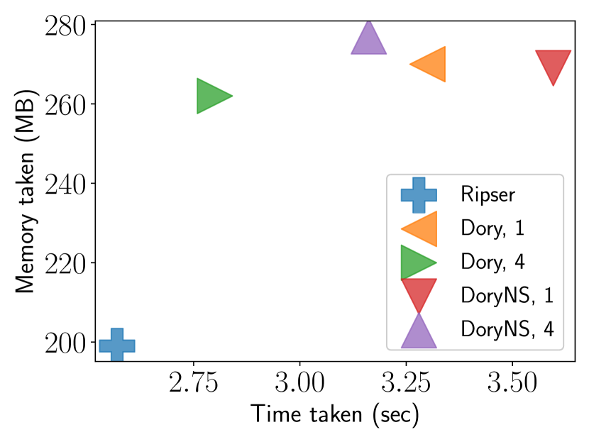
(a) dragon

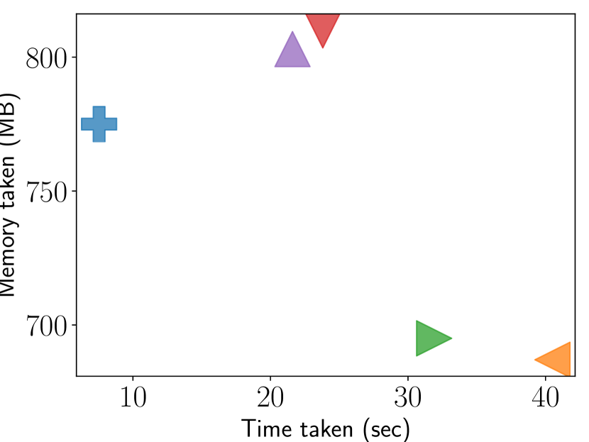
(b) fractal

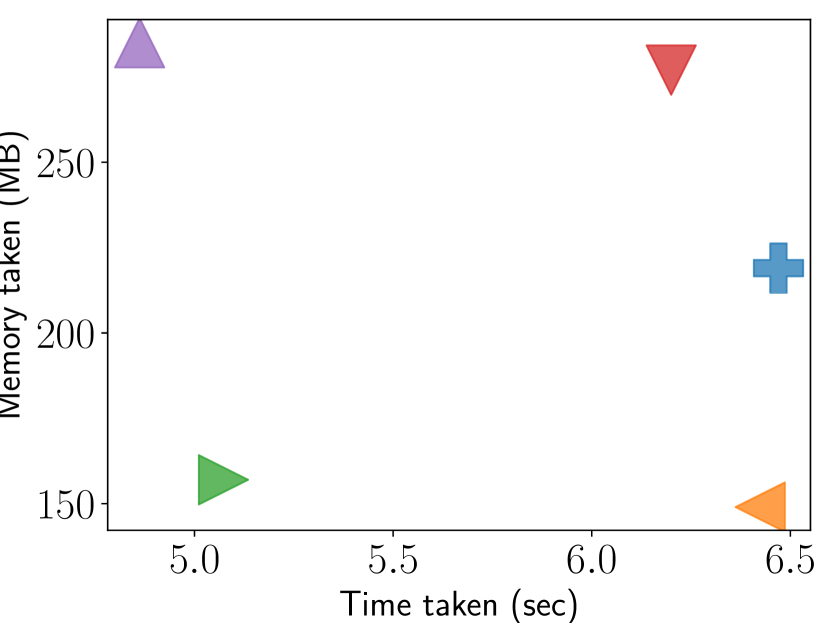
(c) o3

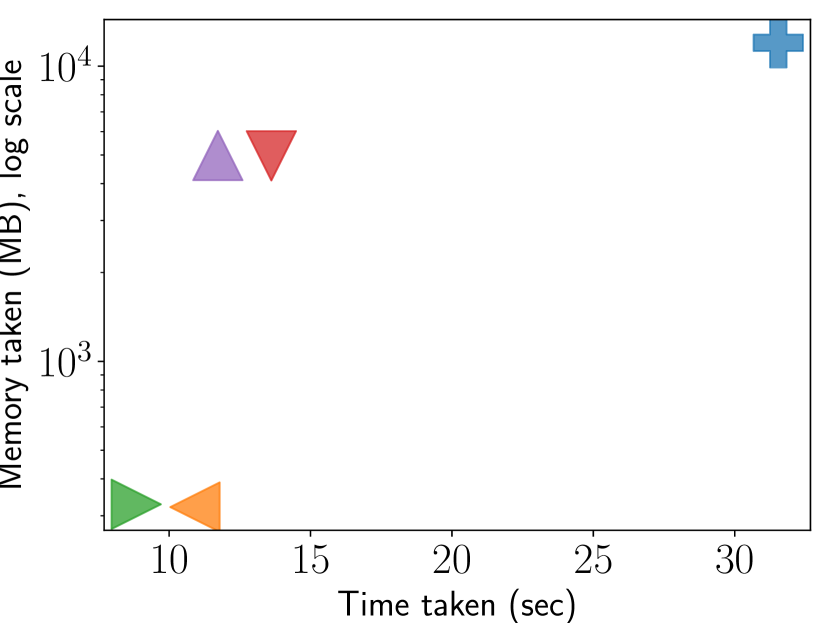
(d) torus4(1)

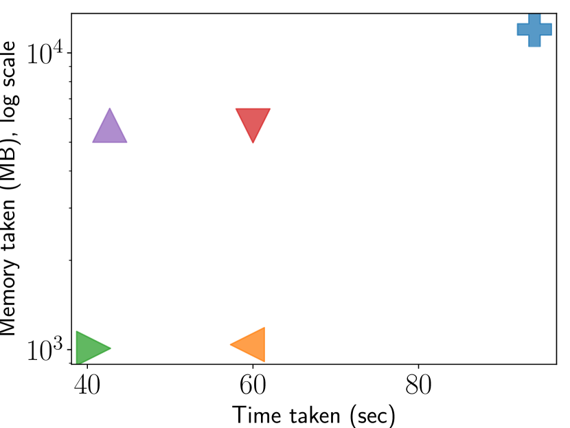
(e) torus4(2)

Figure 18: Computation time and peak memory usage by Dory, DoryNS, and Ripser for the data sets used for benchmarking. The peak memory usage for torus4 data set is shown in log scale. Results for Hi-C data sets are not shown here because only Dory was able to process it.

All PDs are shown in appendices F and G. We observed a discrepancy in the PDs of o3 data set for Gudhi (see Figures 19 and 20), specifically in topological features that do not die. The Gudhi PDs were produced using parameters points = data, max_edge_length = 1 in the method RipsComplex (Python v 3.8.5). In the resulting file, inf entries were replaced by -1 before plotting. The benchmarking and plotting codes can be found at https://github.com/nihcompmed/Dory. We did not explore features of Gudhi, for example, the edge collapse option, that might improve its efficiency or give a consistent PD.

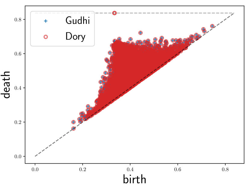
(a) Gudhi

(b) Eirene

(c) Ripser

Figure 19: o3 H₁ PD: Gudhi does not report one feature that does not die and is reported by other algorithms.

(a) Gudhi

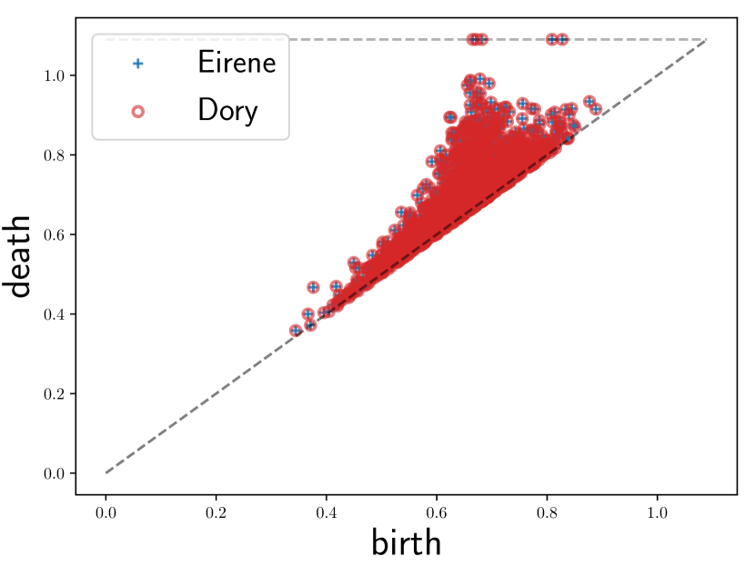
(b) Eirene

(c) Ripser

Figure 20: o3 H₂ PD: Gudhi does not report two features that do not die and are reported by other algorithms.

6 Topology of Human Genome

Among different techniques to quantify chromatin structure, Hi-C experiments allow relatively unbiased measurements across an entire genome (Lieberman-Aiden et al., 2009). Hi-C is based on chromosome conformation capture (3C) which attempts to determine spatial proximity in the cell nucleus between pairs of genetic loci. The experiments measure the interaction frequency of every pair of loci on the genome, and this is believed to correlate with spatial distance in the cell nucleus (Lieberman-Aiden et al., 2009; Dixon et al., 2012).

Using Hi-C experiments, Rao et al. (2014) identified chromatin loops in mouse lymphoblast cells which are orthologous to loops in human lymphoblastoid cells. To highlight the functional importance of chromatin loops they provide multiple sources of evidence that associate most of the detected loops with gene regulation. Rao et al. (2017) showed that treatment of DNA with auxin removes most loop domains.

We test this result by computing PH to compare the number of loops (and voids) across the Hi-C data sets from two different experimental conditions—with and without auxin treatment, provided in Rao et al. (2017). To compute PH, the DNA is visualized as a point-cloud where each point represents a contiguous segment of a 1000 base pairs on a chromosome, a so-called genomic bin. The relative pairwise spatial distances between genomic bins are then estimated from the Hi-C data set at this 1 kilobase resolution. The functionally significant loops in this point-cloud are most likely the ones with spatially close genomic bins on their boundary to allow for biological interaction via physical processes such as diffusion. Therefore, we compute PH up to a low $\tau_{m}$ resulting in a sparse filtration.

In Figure 21, we plot the percentage change in the number of loops and voids upon addition of auxin ($(\beta_{i}^{\text{auxin}}-\beta_{i}^{\text{control}})/\beta_{i}^{\text{control}}*100$). It shows that there is a significant decrease in the number of loops, corroborating previous results (Rao et al., 2017). The analysis using PH additionally shows that the percentage of reduction in the number of loops is greater for thresholds less than 50 and between 100 and 200, and it also shows that most voids are not born when auxin is added. These results warrant an investigation into possible biological implications. The PDs are shown in appendix G.

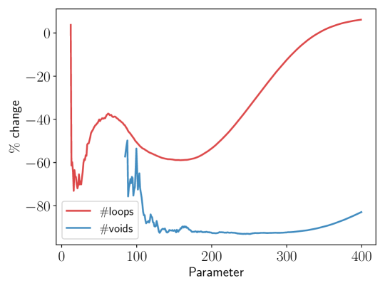
Figure 21: PH of the entire human genome at 1 kilobase resolution shows that the number of loops and voids decreases significantly upon addition of auxin.

7 Discussion

In this paper we introduced a new algorithm that overcomes computational limitations that have prevented the application of PH to large data sets. Compared with pre-existing algorithms, Dory provides significant improvements in memory requirements, without an impractical increase in the computation time. Dory is able to process the large Hi-C data set for the human genome at high resolution, corroborating the expected topology changes of chromatin in different experimental conditions.

While our algorithm is limited to computing PH for VR-filtrations up to three dimensions, a large class of real-world scientific data sets requires only such dimensional restrictions. The current implementation of the algorithm computes PH modulo 2, but it can be easily extended to any prime field.

An alternate class of methods deals with large data sets by approximating their PDs. For example, SimBa (Dey et al., 2019) reduces the number of simplices in the filtration by approximating it to a sparse filtration such that the PDs of the sparse filtration are within a theoretical error of margin when compared to those of the original filtration. Another method, PI-Net (Som et al., 2020), uses neural networks to predict persistence images, that are pixelated approximations of PDs in $\mathbb{R}^{2}.$ The former method uses Gudhi to compute PDs of the approximated sparse filtrations and the latter uses Ripser to compute true PDs when training the neural network. Since Dory can handle larger data sets compared to both Gudhi and Ripser, SimBa and PI-Net can expand their scope by using Dory instead.

In this paper we have focused on computing PDs. However, our algorithm can also be extended to compute representative boundaries of the holes and voids in the data set. For scientific applications, these representative boundaries of topological features in the data set are critical for connecting topology to structural properties of the data that may be linked to functional properties of the underlying system. For instance, they might yield insights into the biological implications of a reduction in the number of voids in human genome upon treatment with auxin. Computation of representative boundaries faces the hurdle of high memory cost. We are currently working on developing a scalable algorithm.

Appendix A Standard Row and Column Algorithms

1:for $j:2\textrm{ to }N$ do

2:     $i\leftarrow 1$

3:     while $i<j$ do

4:         if $\text{low}(j)=\text{pivot}(i)$ then

5:              column $j\leftarrow\text{column }j\oplus\text{column }i$

6:              if column $j$ is empty then

7:                  $\text{low}(j)\leftarrow-1$$\triangleright$ this column is reduced to $\mathbf{0}$

8:                  break

9:              else

10:                  $i\leftarrow 1$               

11:         else

12:              $i\leftarrow i+1$               

13:     $\text{pivot}(j)\leftarrow\text{low}(j)$

Algorithm 4 Standard column algorithm

1:for $i:N\textrm{ to }1$ do

2:     for $j:1\textrm{ to }N$ do

3:         if $\text{low}(j)=i$ then break               

4:     if $j=N+1$ then continue      

5:     $\text{pivot}(j)=\text{low}(j)$

6:     for $k=j+1\textrm{ to }N$ do

7:         if $\text{low}(k)=i$ then

8:              $\text{column }k\leftarrow\text{column }k\oplus\text{column }j$

9:              if column $k$ is empty then

10:                  $\text{low}(k)\leftarrow-1$$\triangleright$ this column is reduced to $\mathbf{0}$

11:                  $\text{pivot}(k)\leftarrow-1$                             

Algorithm 5 Standard row algorithm

Appendix B Algorithms to Compute Cohomology for Edges

1:Input: $(e,i_{a},i_{b},\delta_{e})$

2:Output: $(e,i_{a},i_{b},\delta_{e})$

3:$\{a,b\}\leftarrow f_{1}^{-1}(e)$

4:while $i_{a}<N(a)$ AND $i_{b}<N(b)$ do

5:     if $f_{0}(n^{a}_{i_{a}})<f_{0}(n^{b}_{i_{b}})$ then

6:         $i_{a}\leftarrow i_{a}+1$

7:     else if $f_{0}(n^{a}_{i_{a}})>f_{0}(n^{b}_{i_{b}})$ then

8:         $i_{b}\leftarrow i_{b}+1$

9:     else

10:         return $(e,i_{a},i_{b},\langle f_{1}(\{a,b\}),n^{a}_{i_{a}}\rangle)$      

11:return $(e,i_{a},i_{b},\text{Empty})$ $\triangleright$ Move to case 2

Algorithm 6 Case 1 for edges

1:Input: $(e,i_{a},i_{b},\delta_{e})$

2:Output: $(e,i_{a},i_{b},\delta_{e})$

3:$\{a,b\}\leftarrow f_{1}^{-1}(e)$

4:while $i_{a}<N(a)$ AND $i_{b}<N(b)$ do

5:     if $f_{1}(e^{a}_{i_{a}})<f_{1}(e^{b}_{i_{b}})$ then

6:         $\{a,d\}\leftarrow f_{1}^{-1}(e^{a}_{i_{a}})$

7:         if $d\in N^{b}$ AND $f_{1}(\{b,d\})<f_{1}(e^{a}_{i_{a}})$ then

8:              return $(e,i_{a},i_{b},\langle f_{1}(e^{a}_{i_{a}}),d\rangle)$

9:         else

10:              $i_{a}\leftarrow i_{a}+1$          

11:     else

12:         $\{b,d\}\leftarrow f_{1}^{-1}(e^{b}_{i_{b}})$

13:         if $d\in N^{a}$ AND $f_{1}(\{a,d\})<f_{1}(e^{b}_{i_{b}})$ then

14:              return $(e,i_{a},i_{b},\langle f_{1}(e^{b}_{i_{b}}),d\rangle)$

15:         else

16:              $i_{b}\leftarrow i_{b}+1$               

17:while $i_{a}<N(a)$ do

18:     $\{a,d\}\leftarrow f_{1}^{-1}(e^{a}_{i_{a}})$

19:     if $d\in N^{b}$ AND $f_{1}(\{b,d\})<f_{1}(e^{a}_{i_{a}})$ then

20:         return $(e,i_{a},i_{b},\langle f_{1}(e^{a}_{i_{a}}),d\rangle)$

21:     else

22:         $i_{a}\leftarrow i_{a}+1$      

23:while $i_{b}<N(b)$ do

24:     $\{b,d\}\leftarrow f_{1}^{-1}(e^{b}_{i_{b}})$

25:     if $d\in N^{a}$ AND $f_{1}(\{a,d\})<f_{1}(e^{b}_{i_{b}})$ then

26:         return $(e,i_{a},i_{b},\langle f_{1}(e^{b}_{i_{b}}),d\rangle)$

27:     else

28:         $i_{b}\leftarrow i_{b}+1$      

29:return $(e,i_{a},i_{b},\text{Empty})$

Algorithm 7 Case 2 for edges

1:Input: $e$

2:Output: $(e,i_{a},i_{b},\delta_{e})$

3:$\{a,b\}\leftarrow f_{1}^{-1}(e)$

4:$i_{a}\leftarrow 0$

5:$i_{b}\leftarrow 0$

6:$\delta^{e}_{0}\leftarrow$ Empty

7:$(e,i_{a},i_{b},\delta_{e})\leftarrow$ Function Case1$((e,i_{a},i_{b},\delta_{e}))$

8:if $low$ is Empty then

9:     $i_{a}\leftarrow$ smallest index s.t. $f_{1}(e^{a}_{i_{a}})>f_{1}(e)$

10:     $i_{b}\leftarrow$ smallest index s.t. $f_{1}(e^{b}_{i_{b}})>f_{1}(e)$

11:     $(e,i_{a},i_{b},\delta_{e})\leftarrow$ Function Case2$((e,i_{a},i_{b},\delta_{e}))$

12:return $(e,i_{a},i_{b},\delta_{e})$

Algorithm 8 FindSmallestt

1:Input: $(e,i_{a},i_{b},\delta_{e})$

2:Output: $(e,i_{a},i_{b},\delta_{e})$

3:$\{a,b\}\leftarrow f_{1}^{-1}(e)$

4:$\langle k^{p},k^{s}\rangle\leftarrow\delta^{e}_{i}$

5:if $k^{p}=f_{1}(e)$ then

6:     Increment $i_{a},i_{b}$ by 1

7:     $(e,i_{a},i_{b},\delta^{e}_{i+1})\leftarrow$ Function Case1$((e,i_{a},i_{b},\delta^{e}_{i}))$

8:     if $\delta^{e}_{i+1}$ is Empty then

9:         $i_{a}\leftarrow$ smallest index s.t. $f_{1}(e^{a}_{i_{a}})>f_{1}(e)$

10:         $i_{b}\leftarrow$ smallest index s.t. $f_{1}(e^{b}_{i_{b}})>f_{1}(e)$

11:     else

12:         return $(e,i_{a},i_{b},\delta_{e})$      

13:else

14:     $f_{1}(e^{a}_{i_{a}})<f_{1}(e^{a}_{i_{b}})\,?\,\text{increment }i_{a}:\text{increment }i_{b}$

15:$(e,i_{a},i_{b},\delta_{e})\leftarrow$ Function Case2$((e,i_{a},i_{b},\delta_{e}))$

16:return $(e,i_{a},i_{b},\delta_{e})$

Algorithm 9 FindNextt

1:Input: $e,\delta_{\#}$

2:Output: $(e,i_{a},i_{b},\delta_{e})$

3:$\{a,b\}\leftarrow f_{1}^{-1}(e)$

4:$\langle k^{p},k^{s}\rangle\leftarrow\delta_{\#}$

5:if $k^{p}<f_{1}(e)$ then

6:     $(e,i_{a},i_{b},\delta_{e})\leftarrow$ Function FindSmallestt$(e)$

7:     return $(e,i_{a},i_{b},\delta_{e})$

8:else if $k^{p}=f_{1}(e)$ then

9:     $i_{a}\leftarrow$ smallest index s.t. $f_{0}(n^{a}_{i_{a}})\geq k^{s}$

10:     $i_{b}\leftarrow$ smallest index s.t. $f_{0}(n^{b}_{i_{b}})\geq k^{s}$

11:     if $f_{0}(n^{a}_{i_{a}})=f_{0}(n^{b}_{i_{b}})$ then

12:         return $(e,i_{a},i_{b},\langle k^{p},f_{0}(n^{a}_{i_{a}})\rangle))$

13:     else

14:         $(e,i_{a},i_{b},\delta_{e})\leftarrow$ Function FindNextt$((e,i_{a},i_{b},\text{Empty}))$

15:         if $\delta_{e}$ is not Empty then

16:              return $(e,i_{a},i_{b},\delta_{e})$               

17:$i_{a}\leftarrow$ smallest index s.t. $f_{1}(e^{a}_{i_{a}})\geq k^{p}$

18:$i_{b}\leftarrow$ smallest index s.t. $f_{1}(e^{b}_{i_{b}})\geq k^{p}$

19:if $\langle k^{p},k^{s}\rangle$ is in $\delta e$ then

20:     return $(e,i_{a},i_{b},\langle k^{p},k^{s}\rangle)$

21:$(e,i_{a},i_{b},\delta_{e})\leftarrow$ Function Case2$((e,i_{a},i_{b},\delta_{e}))$

22:return $(e,i_{a},i_{b},\delta_{e})$

Algorithm 10 FindGEQt

Appendix C Algorithms to Compute Coboundary of Triangles

1:Input: $(t,i_{a},i_{b},i_{c},f,\delta_{t})$

2:Output: 1 or 0

3:$\langle k^{p},k^{s}\rangle\leftarrow f_{2}(t)$

4:$a\leftarrow$ min$\{f_{1}^{-1}(k^{p})\}$

5:$b\leftarrow$ max$\{f_{1}^{-1}(k^{p})\}$

6:$c\leftarrow k^{s}$

7:while $i_{c}<N(a)$ AND $f_{1}(e^{c}_{i_{c}})<k^{p}$ do

8:     $\{c,d\}\leftarrow e^{c}_{i_{c}}$

9:     if $f_{1}(\{a,d\})$ and $f_{1}(\{b,d\})$ are less than $k^{p}$ then

10:         $f\leftarrow 0$

11:         $\delta_{t}\leftarrow\langle k^{p},f_{1}(e^{c}_{i_{c}})\rangle$

12:         return 1      

13:     $i_{c}\leftarrow i_{c}+1$

14:return 0

Algorithm 11 Case1 for triangles

1:Input: $(t,i_{a},i_{b},i_{c},f,\delta_{t})$

2:$\langle k^{p},k^{s}\rangle\leftarrow f_{2}(t)$

3:$a\leftarrow$ min$\{f_{1}^{-1}(k^{p})\}$

4:$b\leftarrow$ max$\{f_{1}^{-1}(k^{p})\}$

5:$c\leftarrow k^{s}$

6:while not reached end of all $E^{a},E^{b},E^{c}$ do

7:     $o_{*}\leftarrow\text{min}\{f_{1}(e^{a}_{i_{a}}),f_{1}(e^{b}_{i_{b}}),f_{1}(e^{c}_{i_{c}})\}$$\triangleright$ Exclude indices that reach end of edge-nbd

8:     $\{v_{1},d\}\leftarrow f_{1}^{-1}(o_{*})$

9:     $\{v_{2},v_{3}\}\leftarrow\{a,b,c\}\setminus\{v_{1}\}$

10:     if $f_{1}(\{v_{2},d\})$ and $f_{1}(\{v_{3},d\})$ are less than $o_{*}$ then

11:         $\delta_{t}\leftarrow\langle o_{*},f_{1}(\{v_{2},v3_{\}})\rangle$

12:         $f\leftarrow$ 1 if $v_{1}=a$; 2 if $v_{1}=b$; 3 if $v_{1}=c$

13:         return

14:     else

15:         Increment $i_{v_{1}}$      

16:$\delta_{t}\leftarrow$ Empty

17:$f\leftarrow-1$

Algorithm 12 Case 2 for triangles

1:Input: $(t,i_{a},i_{b},i_{c},f,\delta_{t})$

2:$i_{c}\leftarrow 0$

3:if Function Case1$(t,i_{a},i_{b},i_{c},f,\delta_{t})$ then

4:     return

5:$\langle k^{p},k^{s}\rangle\leftarrow t$

6:$\{a,b\}\leftarrow f_{1}^{-1}(k^{p})$

7:$i_{a}\leftarrow\operatorname*{argmin}\limits_{i_{a}}(f_{1}(e^{a}_{i_{a}})\geq k^{p})$

8:$i_{b}\leftarrow\operatorname*{argmin}\limits_{i_{b}}(f_{1}(e^{b}_{i_{b}})\geq k^{p})$

9:Increment $i_{a},i_{b}$

10:Function Case2$(t,i_{a},i_{b},i_{c},f,\delta_{t})$

Algorithm 13 FindSmallesth

1:Input: $(t,i_{a},i_{b},i_{c},f,\delta_{t})$

2:$\langle k^{p},c\rangle\leftarrow f_{2}(t)$

3:$a\leftarrow$ min$\{f_{1}^{-1}(k^{p})\}$

4:$b\leftarrow$ max$\{f_{1}^{-1}(k^{p})\}$

5:$c\leftarrow k^{s}$

6:if $f=0$ then

7:     Increment $i_{c}$

8:     if Function Case1 $(t,i_{a},i_{b},i_{c},f,\delta_{t})$ then

9:         return      

10:     $i_{a}\leftarrow\operatorname*{argmin}\limits_{i_{a}}(f_{1}(e^{a}_{i_{a}})\geq k^{p})$

11:     $i_{b}\leftarrow\operatorname*{argmin}\limits_{i_{b}}(f_{1}(e^{b}_{i_{b}})\geq k^{p})$

12:     Increment $i_{a},i_{b}$

13:if Not moving from Case1 then

14:     if $f=1$ then

15:         $i_{a}\leftarrow i_{a}+1$

16:     else if $f=2$ then

17:         $i_{b}\leftarrow i_{b}+1$

18:     else if $f=3$ then

19:         $i_{c}\leftarrow i_{c}+1$      

20:Function Case2$(t,i_{a},i_{b},i_{c},f,\delta_{t})$

Algorithm 14 FindNexth for triangles

1:Input: $(t,i_{a},i_{b},i_{c},f,\delta_{t}),\delta_{\#}$

2:$\langle k^{p}_{\#},k^{s}_{\#}\rangle\leftarrow\delta_{\#}$

3:$\langle k^{p},c\rangle\leftarrow t$

4:$\{a,b\}\leftarrow f_{1}^{-1}(k^{p})$

5:if $k^{p}_{\#}<k^{p}$ then

6:     Function FindSmallesth$(t,i_{a},i_{b},i_{c},f,\delta_{t})$

7:     return

8:else if $k^{p}_{\#}=k^{p}$ then

9:     $i_{c}\leftarrow\operatorname*{argmin}\limits_{i_{c}}(f_{1}(e^{c}_{i_{c}})\geq k^{s}_{\#})$

10:     if $f_{1}(e^{c}_{i_{c}})=k^{s}_{\#}$ then

11:         $\delta_{t}\leftarrow\delta_{\#}$

12:         $v\leftarrow 0$

13:         return      

14:     if Function Case1$(t,i_{a},i_{b},i_{c},f,\delta_{t})$ then

15:         return      

16:     $i_{a}\leftarrow\operatorname*{argmin}\limits_{i_{a}}(f_{1}(e^{a}_{i_{a}})\geq k^{p})$

17:     $i_{b}\leftarrow\operatorname*{argmin}\limits_{i_{b}}(f_{1}(e^{b}_{i_{b}})\geq k^{p})$

18:     Increment $i_{a},i_{b}$

19:else

20:     $i_{a}\leftarrow\operatorname*{argmin}\limits_{i_{a}}(f_{1}(e^{a}_{i_{a}})\geq k^{p}_{o})$

21:     $i_{b}\leftarrow\operatorname*{argmin}\limits_{i_{b}}(f_{1}(e^{b}_{i_{b}})\geq k^{p}_{o})$

22:     $i_{c}\leftarrow\operatorname*{argmin}\limits_{i_{c}}(f_{1}(e^{c}_{i_{c}})\geq k^{p}_{o})$

23:while 1 do

24:     Function Case2$(t,i_{a},i_{b},i_{c},f,\delta_{t})$

25:     if $\delta_{t}\geq\delta_{\#}$ OR $\delta_{t}$ is Empty then

26:         break      

27:     if $f=1$ then

28:         $i_{a}\leftarrow i_{a}+1$

29:     else if $f=2$ then

30:         $i_{b}\leftarrow i_{b}+1$

31:     else if $f=3$ then

32:         $i_{c}\leftarrow i_{c}+1$      

Algorithm 15 FindGEQh for triangles

Appendix D Algorithms for Serial-parallel Cohomology Reduction of Triangles

1:Function SerialParallelReduce

2:     Function ParallelReduce

3:     Function SerialReduce

4:     Function Clearance

5:EndFunction

6:

7:Input $F_{1},$ batch-size

8:$V^{\bot},\mathbf{v}\leftarrow[\,]$

9:$i\leftarrow 0$

10:for $e$ in $F^{-1}_{1}$ do

11:     Compute $\delta e$ and sort it along $F^{-1}_{2}$

12:     for $t$ in $\delta e$ with $d(t)=e$ do

13:         $(t,i_{a},i_{b},i_{c},f,\delta_{t})\leftarrow$ Function FindSmallesth$(t)$

14:         if $\delta^{t}_{1}$ is Empty then

15:              continue          

16:         $v_{i}\leftarrow[(t,i_{a},i_{b},i_{c},f,\delta_{t})]$

17:         $\delta^{v_{i}}_{*}\leftarrow\delta_{t}$

18:         $f_{e}\leftarrow 0$

19:         Append $(t,v_{i},\delta^{v_{i}}_{*},f_{v},f_{r},f_{a},f_{e})$ to $\mathbf{v}$

20:         $i\leftarrow i+1$

21:         if $i=$ batch-size then

22:              Function SerialParallelReduce               

23:

24:while $i>0$ do

25:     Function SerialParallelReduce

Algorithm 16 SerialParallel: Reduction of triangles

1:Input: $\mathbf{v},V^{\bot},p^{\bot}$

2:Output: $\mathbf{v}$

3:for $(t,v_{i},\delta^{v_{i}}_{*},f_{v},f_{r},f_{a},f_{e})$ in $\mathbf{v}$ do$\triangleright$ Embarrassingly parallel

4:     $f_{r}\leftarrow 0$

5:     $f_{a}\leftarrow 1$

6:     if $(\delta^{v_{i}}_{*},t)$ is a trivial persistence pair then

7:         continue      

8:     while $(\delta^{v_{i}}_{*},t^{\prime})$ is a trivial persistence pair OR is in $p^{\bot}$ do

9:         $(t^{\prime},i_{a},i_{b},i_{c},v,\delta_{t^{\prime}})\leftarrow$ Function FindGEQt$(t^{\prime},\delta^{v_{i}}_{*})$

10:         Append $(t^{\prime},i_{a},i_{b},i_{c},f,\delta_{t^{\prime}})$ to $v_{i}$

11:         for $t_{k}$ in $V^{\bot}(t^{\prime})$ do

12:              $(t_{k},i_{a},i_{b},i_{c},f,\delta_{t_{k}})\leftarrow$ Function FindGEQt$(t_{k},\delta^{v_{i}}_{*})$

13:              Append $[(t_{k},i_{a},i_{b},i_{c},f,\delta_{t_{k}})]$ to $v_{i}$          

14:         Implicit column algorithm to update $\delta_{*}^{v_{i}}$

15:         if $\delta^{v_{i}}_{*}$ is Empty then

16:              $f_{e}\leftarrow 1$

17:              return               

Algorithm 17 Parallel reduction

1:for $(t,v_{i},\delta^{v_{i}}_{*},f^{i}_{r},f^{i}_{v},f^{i}_{a},f^{i}_{e})$ in $\mathbf{v}$ do

2:     if $f^{i}_{e}$ OR $f^{i}_{v}$ then

3:         continue      

4:     $j\leftarrow 1$

5:     while $j<i$ do

6:         if $f^{j}_{e}$ then

7:              $j\leftarrow j+1$

8:              continue          

9:         if $\delta^{v_{j}}_{*}>\delta^{v_{i}}_{*}$ then

10:              $j\leftarrow j+1$

11:              continue          

12:         if $\delta^{v_{j}}_{*}<\delta^{v_{i}}_{*}$ then

13:              if $f^{j}_{r}$ OR $f^{j}_{v}$ then

14:                  $f^{i}_{a}\leftarrow 0$

15:                  break               

16:              $j\leftarrow j+1$

17:              continue          

18:         Append $v_{j}$ to $v_{i}$

19:         Fast implicit column algorithm to update $\delta_{*}^{v_{i}}$

20:         if $\delta^{v_{i}}_{*}$ is Empty then

21:              $f^{i}_{e}\leftarrow 1$

22:              break          

23:         if $\exists t^{\prime}\text{ s.t. }(\delta^{v_{i}}_{*},t^{\prime})$ is a trivial pair then

24:              $f^{i}_{v}\leftarrow 1$

25:              $f^{i}_{r}\leftarrow 0$

26:              $f^{i}_{a}\leftarrow 0$

27:              break          

28:         if $(\delta^{v_{i}}_{*},t^{\prime})$ is a persistence pair in $p^{\bot}$ then

29:              $f^{i}_{v}\leftarrow 0$

30:              $f^{i}_{r}\leftarrow 1$

31:              $f^{i}_{a}\leftarrow 0$

32:              break          

33:         $j\leftarrow 1$      

Algorithm 18 Serial reduction

1:for $(t,v_{i},\delta^{v_{i}}_{*},f_{v},f_{r},f_{a},f_{e})$ in $\mathbf{v}$ do

2:     if $f_{e}=0$ then

3:         Non-contractible cycle born at $t$

4:         Remove $(t,v_{i},\delta^{v_{i}}_{*},f_{v},f_{r},f_{a},f_{e})$ from $\mathbf{v}$

5:         continue      

6:     if $f_{a}=1$ then

7:         Store $(\delta^{v_{i}}_{*},t)$ in $p^{\bot}(t)$

8:         Define $T\leftarrow[t_{k}\text{ in }v_{i}=[(t_{k},i_{a},i_{b},i_{c},f,\delta^{t_{k}}_{*})]\text{ with }t_{k}\neq t]$

9:         Remove triangles from $T$ that occur even number of times (modulo 2 sum)

10:         $V^{\bot}(t)\leftarrow T$

11:         Remove $(t,v_{i},\delta^{v_{i}}_{*},f_{v},f_{r},f_{a},f_{e})$ from $\mathbf{v}$      

Algorithm 19 Clearance

Appendix E Computation and Benchmarks

Base memory used by Dory
$F_{1}:$ (two vertices per edge) $+$ (pointer to every edge) $+$ (length of every edge) $=2n_{e}+n_{e}+n_{e}=4n_{e}.$
Lengths of neighborhoods: one for every vertex $=n.$
Vertex-neighborhood:(every edge is in two neighborhoods)*(neighbor and order are stored) + (pointer for every vertex) $=(2n_{e})*2+n$ $=4n_{e}+n.$
Edge-neighborhood $=$ Vertex-Neighborhood $=4n_{e}+n.$

Fast implicit col and implicit row algorithm

Data set	Fast Imp. col.	Imp. row
dragon	( 2.859 s, 262 MB )	(2.887 s, 270 MB )
fractal	( 32.1 s, 695 MB)	(29.848 s, 670 MB )
o3	( 4.989 s, 157 MB)	( 22.7 s, 140 MB )
torus4(1)	( 9.4 s, 328 MB)	( 44.47 s, 295 MB )
torus4(2)	(41.2 s, 1 GB)	( 74.6 s, 1 GB )
Hi-C (control)	(263 s, 6.23 GB)	( 595 s, 7.19 GB )
Hi-C (Auxin) (102 s, 3.98 GB )	( 123 s, 3.83 GB )

Table 4: Comparing fast implicit column algorithm (Dory compiled with -D SAVEPD) and implicit row algorithm (both serial-parallel over 4 threads). Time taken (seconds) was measured using the command time in terminal of macOS. Peak memory usage is recorded using application Instruments in macOS.

Gudhi and Eirene
The peak memory usage by Gudhi (v. 3.4.0)was recorded using the package memory-profiler (v. 0.57.0) in Python (v. 3.8.5), and the memory used by Eirene (v. 1.3.5) was estimated by observing activity monitor of macOS because the memory profiling tools in Julia (v. 1.5) report cumulative memory allocations instead of the net memory in use.

Data set	$n$	$\tau_{m}$	$d$	Gudhi	Eirene
dragon	2000	$\infty$	1	NA	7.4 GB
fractal	512	$\infty$	2	NA	9.13 GB
o3	8192	1	2	2.3 GB	9.34 GB
torus4(1)	50000	0.15	1	3 GB	126 GB
torus4(2)	50000	0.15	2	30 GB	NA

Table 5: Benchmarks for Gudhi and Eirene. NA means that the data set was not processed within 10 mins. or the system ran out of memory.

Appendix F Persistence Diagrams for Data Sets

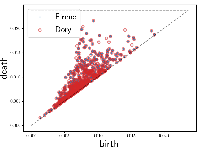
(a) Eirene

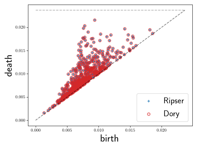
(b) Ripser

Figure 22: Dragon H₁ PD

(a) Eirene

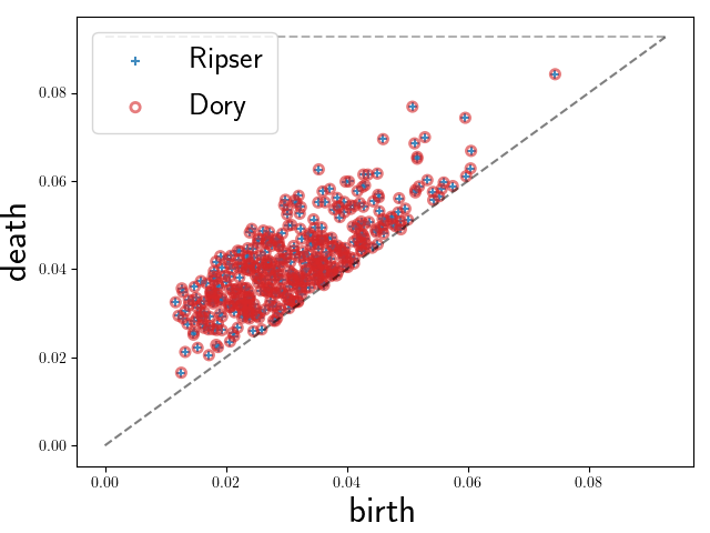
(b) Ripser

Figure 23: Fractal H₁ PD

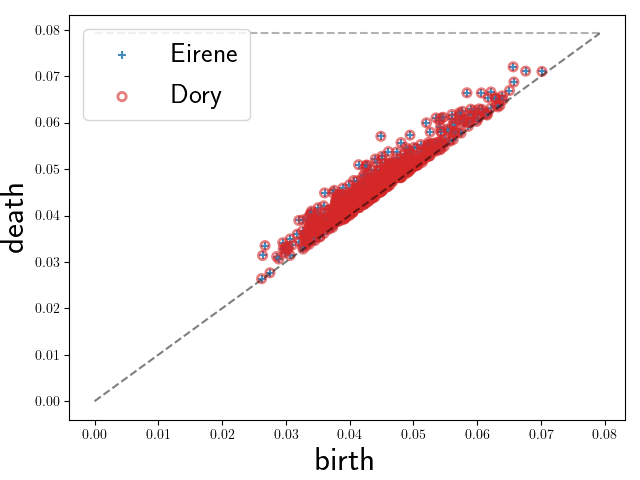
(a) Eirene

(b) Ripser

Figure 24: Fractal H₂ PD

(a) Gudhi

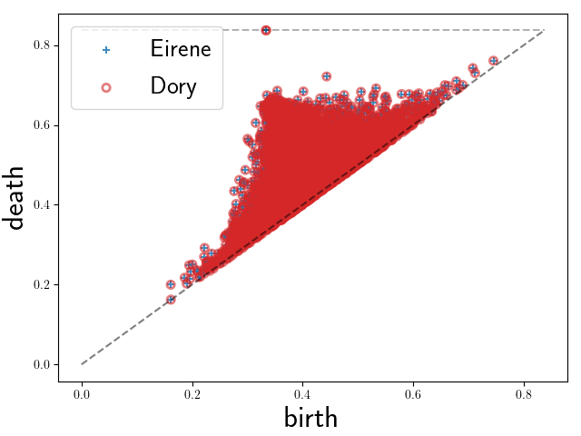
(b) Eirene

(c) Ripser

Figure 25: o3 H₁ PD

(a) Gudhi

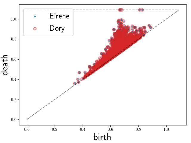
(b) Eirene

(c) Ripser

Figure 26: o3 H₂ PD

(a) Gudhi

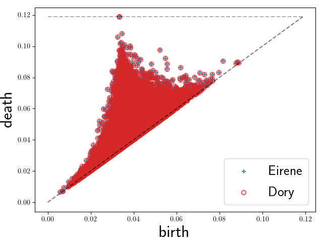
(b) Eirene

(c) Ripser

Figure 27: torus H₂ PD

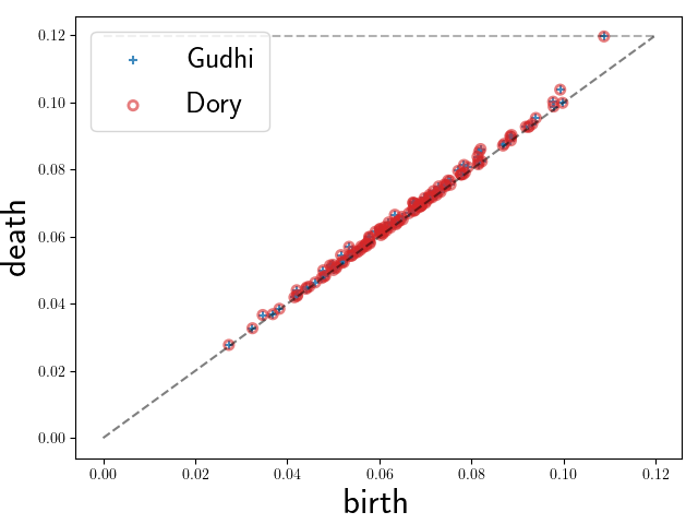
(a) Gudhi

(b) Ripser

Figure 28: torus H₂ PD

Appendix G Persistence Diagrams for Hi-C

(a) Control

(b) Auxin

Figure 29: Hi-C data sets H₁ PD

(a) Control

(b) Auxin

Figure 30: Hi-C data sets H₂ PD

References

- Edelsbrunner and Harer [2008] Herbert Edelsbrunner and John Harer. Persistent homology-a survey. Contemporary mathematics, 453:257–282, 2008.
- De Silva et al. [2011] Vin De Silva, Dmitriy Morozov, and Mikael Vejdemo-Johansson. Dualities in persistent (co) homology. Inverse Problems, 27(12):124003, 2011.
- Boissonnat and Maria [2014] Jean-Daniel Boissonnat and Clément Maria. The simplex tree: an efficient data structure for general simplicial complexes. Algorithmica, 70(3):406–427, 2014.
- Bauer [2019] Ulrich Bauer. Ripser: efficient computation of vietoris-rips persistence barcodes. arXiv preprint arXiv:1908.02518, 2019.
- Rowley and Corces [2018] M Jordan Rowley and Victor G Corces. Organizational principles of 3d genome architecture. Nature Reviews Genetics, 19(12):789–800, 2018.
- Lieberman-Aiden et al. [2009] Erez Lieberman-Aiden, Nynke L Van Berkum, Louise Williams, Maxim Imakaev, Tobias Ragoczy, Agnes Telling, Ido Amit, Bryan R Lajoie, Peter J Sabo, Michael O Dorschner, et al. Comprehensive mapping of long-range interactions reveals folding principles of the human genome. science, 326(5950):289–293, 2009.
- Rao et al. [2014] Suhas SP Rao, Miriam H Huntley, Neva C Durand, Elena K Stamenova, Ivan D Bochkov, James T Robinson, Adrian L Sanborn, Ido Machol, Arina D Omer, Eric S Lander, et al. A 3d map of the human genome at kilobase resolution reveals principles of chromatin looping. Cell, 159(7):1665–1680, 2014.
- Rao et al. [2017] Suhas SP Rao, Su-Chen Huang, Brian Glenn St Hilaire, Jesse M Engreitz, Elizabeth M Perez, Kyong-Rim Kieffer-Kwon, Adrian L Sanborn, Sarah E Johnstone, Gavin D Bascom, Ivan D Bochkov, et al. Cohesin loss eliminates all loop domains. Cell, 171(2):305–320, 2017.
- Edelsbrunner et al. [2000] Herbert Edelsbrunner, David Letscher, and Afra Zomorodian. Topological persistence and simplification. In Proceedings 41st annual symposium on foundations of computer science, pages 454–463. IEEE, 2000.
- Cohen-Steiner et al. [2006] David Cohen-Steiner, Herbert Edelsbrunner, and Dmitriy Morozov. Vines and vineyards by updating persistence in linear time. In Proceedings of the twenty-second annual symposium on Computational geometry, pages 119–126, 2006.
- Chen and Kerber [2011] Chao Chen and Michael Kerber. Persistent homology computation with a twist. In Proceedings 27th European Workshop on Computational Geometry, volume 11, pages 197–200, 2011.
- Otter et al. [2017] Nina Otter, Mason A Porter, Ulrike Tillmann, Peter Grindrod, and Heather A Harrington. A roadmap for the computation of persistent homology. EPJ Data Science, 6(1):17, 2017.
- Dixon et al. [2012] Jesse R Dixon, Siddarth Selvaraj, Feng Yue, Audrey Kim, Yan Li, Yin Shen, Ming Hu, Jun S Liu, and Bing Ren. Topological domains in mammalian genomes identified by analysis of chromatin interactions. Nature, 485(7398):376–380, 2012.
- Dey et al. [2019] Tamal K Dey, Dayu Shi, and Yusu Wang. Simba: An efficient tool for approximating rips-filtration persistence via sim plicial ba tch collapse. Journal of Experimental Algorithmics (JEA), 24:1–16, 2019.
- Som et al. [2020] Anirudh Som, Hongjun Choi, Karthikeyan Natesan Ramamurthy, Matthew P Buman, and Pavan Turaga. Pi-net: A deep learning approach to extract topological persistence images. In Proceedings of the IEEE/CVF Conference on Computer Vision and Pattern Recognition Workshops, pages 834–835, 2020.