Flow Time Scheduling with Uncertain Processing Time

Abstract

We consider the problem of online scheduling on a single machine in order to minimize weighted flow time. The existing algorithms for this problem (STOC ’01, SODA ’03, FOCS ’18) all require exact knowledge of the processing time of each job. This assumption is crucial, as even a slight perturbation of the processing time would lead to polynomial competitive ratio. However, this assumption very rarely holds in real-life scenarios.

In this paper, we present the first algorithm for weighted flow time which do not require exact knowledge of the processing times of jobs. Specifically, we introduce the Scheduling with Predicted Processing Time (sppt) problem, where the algorithm is given a prediction for the processing time of each job, instead of its real processing time. For the case of a constant factor distortion between the predictions and the real processing time, our algorithms match all the best known competitiveness bounds for weighted flow time – namely $O(\log P),O(\log D)$ and $O(\log W)$, where $P,D,W$ are the maximum ratios of processing times, densities, and weights, respectively. For larger errors, the competitiveness of our algorithms degrades gracefully.

1 Introduction

The field of online scheduling focuses on efficient processing of jobs by machines, where the jobs are not known in advance but are released over time. An algorithm in this setting must assign each job to a machine, which must then process the job for some specific amount of time (called the processing time of the job).

In a classic setting for online scheduling, the algorithm is given a single machine, and aims to minimize the total flow time: the sum over jobs of the time that the job was pending in the algorithm (i.e. the difference between its completion time and its release time). In this setting, we usually allow preemption of a currently-processed job, which is pausing its processing until some future time, in which the processing will resume from the state in which it was paused. A classic result by Smith from 1956 [20] shows that this problem can be solved optimally using the SRPT (shortest remaining processing time) schedule.

A natural generalization of the total flow time metric is total weighted flow time, in which each job also has a weight. The goal is therefore to minimize the weighted sum of flow times, where the weight of a job is the weight of its flow time in the goal function. While natural, this problem has proved much harder than minimizing unweighted flow time: the best known algorithms [3, 1] have competitive ratios with logarithmic dependence on various parameters of the input; such parameters include the ratio $P$ of the largest to smallest processing time in the input, the ratio $W$ of the largest to smallest job weight in the input, and the ratio $D$ of the largest to smallest density in the input (where the density of a job is the ratio of its weight to its processing time). As shown by Bansal and Chan [2], a dependence on these parameters is necessary (without added leniency such as speed augmentation).

However, these algorithms for both weighted and unweighted flow time make the assumption that the processing time of a job becomes known to the algorithm upon the release of the job. This assumption almost never holds in real-world scenarios, as nearly all computer programs of some complexity have varying running times. In the case of weighted flow-time, this assumption is ubiquitous – it is crucial to all known algorithms of sub-polynomial competitiveness [8, 3, 1], as replacing the real processing time with the predicted processing time in those algorithms would yield polynomial competitive ratios (e.g. $\Omega(P)$) even for a slight misprediction by a factor of $1+\epsilon$ (compare this to the original polylogarithmic competitiveness of those algorithms).

Predicted Processing Time and Robustness.

While knowing the exact processing time is infeasible in a real-world scenario, one could hold a prediction for the processing time of a job, of varying accuracy. Such predictions might be obtained from machine-learning algorithms, simple heuristics, or any other source. A good algorithm in this setting would be able to perform well given only the prediction, rather than the actual procesing time, upon the release of a job.

The fact that the known guarantees for scheduling problems apply only for algorithms that know the processing time completely creates a gap between theory and practice. In this paper, we address this gap. Namely, we introduce the model of scheduling with predicted processing time (sppt), in which upon the release of a job, we are provided with a prediction of the job’s processing time. An instance of the problem is characterized by a distortion parameter, which is the maximum ratio over jobs of the job’s real processing time and its predicted processing time.

In this paper, we present competitive algorithms which are $\mu$-robust; that is, they maintain their competitive ratio guarantees for all inputs with distortion parameter at most $\mu$. The competitive ratios have a polynomial dependency on $\mu$ (contrast with previously-known algorithms, where the competitive ratio immediately degrades to e.g. $\Omega(P)$ even when $\mu=1+\epsilon$ for a small $\epsilon$). We assume that a value for the single parameter $\mu$ that bounds the distortion of the input can be learned, in order to apply the correct robust algorithm; the case in which this assumption does not hold seems surprisingly tricky, and is discussed in Section 5.

At this point, one might ask whether the definition of the distortion parameter as the maximum distortion is indeed the correct measure for the error of the prediction; for example, could guarantees in some average of errors, e.g. geometric, be given? However, our choice of maximum distortion is not overly-conservative, but rather prescribed by the nature of the flow-time metric – specifically, due to its sensitivity to bad local competitive ratio. Consider for example, a scheduling instance which initially releases jobs with very erroneous, which would cause the algorithm to perform badly at some point in time. The adversary could then maintain this bad perform by releasing a stream of very short jobs; this well-known “bombardment” technique would guarantee a bad (global) competitive ratio for the algorithm. However, the processing time of these short “bombardment” jobs could be predicted with full accuracy, yielding a geometric average of errors which is arbitrarily close to $1$ as the “bombardment” continues; this would also be the case for every other reasonable average.

1.1 Our Results

The sppt Problem.

We present algorithms for sppt for minimizing weighted flow time. An algorithm, coupled with some competitiveness guarantee, is called $\mu$-robust if its competitiveness guarantee is achieved for any instance with distortion parameter at most $\mu$ (and not only for inputs where the prediction matches the real processing time).

Without loss of generality, we assume one-sided error: that is, that the real processing time of each job is at least the predicted processing time, and at most $\mu$ times the predicted processing time. This one-sided error can be trivially obtained from a two-sided error with distortion parameter $\mu^{\prime}$ by dividing each prediction by the distortion parameter $\mu^{\prime}$; the new distortion parameter $\mu$ of the new one-sided-error instance would be at most $(\mu^{\prime})^{2}$.

Recall that $P,D,W$ are the ratios of maximum to minimum processing time, density and weight, respectively. For any $\mu$, our results are:

1. A $\mu$-robust algorithm for sppt with weighted flow time, which is simultaneously $O(\mu^{3}\log(\mu P))$-competitive and $O(\mu^{3}\log(\mu D))$-competitive.

2. A $\mu$-robust algorithm for sppt with weighted flow time, which is $O(\mu^{2}\log W)$-competitive.

In the process of designing the $O(\mu^{2}\log W)$-competitive algorithm, we also design a $\mu$-robust algorithm for sppt with unweighted flow time, which is $2\left\lceil{\mu}^{2}\right\rceil$-competitive. Note that, somewhat surprisingly, even for $\mu$ arbitrarily close to $1$, there exists a lower bound of $2$ on the competitiveness of any deterministic $\mu$-robust algorithm, which we show in Appendix C.

For the weighted setting, and for a constant $\mu$, our algorithms match the best known results in terms of all three parameters: the $O(\log W)$-competitive algorithm of Bansal and Dhamdhere [3], and the $O(\log P)$ and $O(\log D)$ competitive algorithms in [1]. Even for distortion significantly larger than constant, e.g. $\mu=\Theta(\log P)$, our algorithms still obtain polylogarithmic competitiveness.

A special case of sppt is the problem of semiclairvoyant scheduling [7, 6]. In this problem, instead of getting the processing time $p_{q}$ of a job $q$, we are given its class, which is $\ell_{q}=\left\lfloor\log_{\rho}p_{q}\right\rfloor$ for some constant $\rho>1$. Applying our algorithms for sppt we obtain the first semiclairvoyant algorithms for weighted flow time, which match the best known guarantees for the clairvoyant setting. As a side result, we also obtain an improvement to the best known result for unweighted flow time. The exact statement of our results for the semiclairvoyant setting are given in Appendix D.

Paper Structure.

The $\mu$-robust algorithm with logarithmic dependency on either $P$ or $D$ is presented in Section 3. The $\mu$-robust algorithm with logarithmic dependency on $W$ is shown in Section 4. Section 4 comprises two subsections: Subsection 4.1 presents a $\mu$-robust algorithm for the unweighted setting, while Subsection 4.2 uses the algorithm of Subsection 4.1 to construct the algorithm for the weighted setting. Appendix C shows a lower bound of $2$-competitiveness for $\mu$-robust algorithms in the unweighted setting, even for vanishingly small distortion. Appendix D discusses the application of the algorithms for sppt to the semiclairvoyant setting.

1.2 Our Techniques

In developing robust algorithms for sppt, we have used orthogonal methods and analyses for the algorithm for $P$ and $D$ and the algorithm for $W$. Curiously, it seems that the techniques of each single algorithm could not be applied to obtain the results of the other algorithm.

The $O(\mu^{3}\log(\mu P))$-competitive algorithm for sppt, which is also $O(\mu^{3}\log(\mu D))$-competitive, is a simply-stated and novel algorithm. The flavor of its analysis is somewhat reminiscent of the $O(\log^{2}P)$-competitive algorithm of Chekuri et al. [8] (though, of course, our analysis shows an improved competitiveness, as our guarantee is $O(\log P)$ when $\mu$ is constant).

The algorithm begins by rounding the weights of jobs up to powers of $\Theta(\mu)$; this is the only place in the algorithm where $\mu$ is used. In weighted flow time, an algorithm must choose whether to prioritize high-weight jobs or cost-effective jobs (high density). The algorithm contends with this issue in the following way: it chooses the maximum weight $w$ of a living job, and then chooses a job from the highest density class such that this class contains at least $w$ weight. Inside this density class, the algorithm always chooses the highest weight job.

In the analysis of this algorithm, we show that the maximum weight in the algorithm never exceeds the total weight in the optimal solution. As for the lower weight classes which the algorithm does use, a volume-based analysis shows that the total weight in those classes is bounded.

The $O(\mu^{2}\log W)$-competitive algorithm for sppt with weighted flow time is completely different in both methods and analysis from the previous algorithm, instead using the analysis framework introduced by Bansal and Dhamdhere [3].

The algorithm is constructed in two steps. First, we introduce a $\mu$-robust algorithm for minimizing unweighted flow time. This algorithm uses two bins to maintain pending jobs, a full bin and a partial bin, which contain roughly the same number of jobs. Only jobs in the partial bin are processed by the algorithm, so that the jobs in the full bin retain their original processing time. Thus, the full bin provides a “counterweight” of full jobs to the partial bin; the intuition for this is that the algorithm wants to limit the fraction of partially-processed jobs at any point in time. Indeed, naive processing without attempting to limit the number of partially-processed jobs would result in unbounded competitive ratio, as observed in [6]. The competitiveness proof of this algorithm bears similarities to the proof framework of Bansal and Dhamdhere [3], also found in [1]. However, both of those papers use SRPT as a crucial component in their algorithms and analyses, which is infeasible in sppt. Thus, our algorithms are designed to bypass this requirement.

When designing the priority of jobs in the full bin, we need to overcome the fact the algorithm does not know the remaining processing times of jobs (prohibiting strategies such as SRPT). Instead, the algorithm identifies and eliminates violations, which are pairs of jobs provably not ordered according to SRPT; this occurs when their predicted processing times differ by more than $\mu$. The algorithm solves violations using a rotation operation, which identifies all violations involving a job and rotates their priorities. The resulting priority sequence, which contains no violations, is “quasi-SRPT” – that is, the upper bound for the processing time of a low-priority job is always higher than the lower bound for the processing time of a high-priority job.

Interestingly, the priority among the jobs in the partial bin is LIFO, which is perhaps counterintuitive. While we are not sure that LIFO is the only option for achieving competitiveness, our proof crucially requires this feature.

We use the robust algorithm for unweighted flow time as a component in the $O(\mu^{2}\log W)$-competitive algorithm for sppt with weighted flow time. This algorithm is composed of multiple full-partial bin pairs, one for each of the $\log W$ weight classes. Each bin pair behaves as an instance of the unweighted algorithm, and the algorithm chooses the heaviest bin pair to process at any given time (more specifically, the bin pair with the heaviest partial bin is processed). The proof framework used for the unweighted algorithm is now utilized, as it naturally supports multiple bin pairs.

One could hope that any $\mu$-robust algorithm for the unweighted setting could be extended (at a loss of $O(\log W)$) to the weighted setting through binning. However, this is not known to be the case for weighted flow time – the binning technique is not black-box, and previous algorithms using binning ([3, 1]) demanded specific properties from the algorithm used in each bin. The main focus in designing the unweighted component of our algorithm is for it to “play nice” with the binning technique; this fact requires a delicate assignment of job priorities.

1.3 Related Work

The first algorithm with polylogarithmic guarantee for minimizing weighted flow time on a single machine was presented by Chekuri et al. [8], which was $O(\log^{2}P)$-competitive. Bansal and Dhamdhere [3] gave an $O(\log W)$-competitive algorithm. Bansal and Chan [2] then showed that any deterministic algorithm for the problem must be $\Omega\left(\min\left\{\sqrt{\frac{\log W}{\log\log W}},\sqrt{\frac{\log\log P}{\log\log\log P}}\right\}\right)$ -competitive, showing that dependence on at least one parameter is necessary. In [1], $O(\log P)$-competitive and $O(\log D)$-competitive algorithms were given, where $D$ is the maximum ratio of densities of jobs (where density is processing time over weight). For more than a single machine, the problem is essentially intractable – Chekuri et al. [8] show a lower bound of $\Omega\left(\min\left\{\sqrt{P},\sqrt{W},(n/m)^{\frac{1}{4}}\right\}\right)$ . With $(1+\epsilon)$ speed augmentation, this problem is significantly easier [11, 3, 21].

The field of combining online algorithms with machine-learned predictions has seen significant interest in the last few years, with some works involving predictions in scheduling. For example, Purohit et al. [19] studied minimizing job completion time with predicted processing time. Other forms of prediction are also used; for example, Lattanzi et al. [12] studied the case of restricted assignment to multiple machines to minimize makespan, and used an algorithm-specific prediction (machine weights). Scheduling with predictions has also been studied in the queueing theory setting [16, 15]. Additional work on algorithms with predictions can be found in [13, 14, 17]

The case in which no prediction is given (and thus the algorithm knows nothing about the processing time of jobs) is called the nonclairvoyant model, and was studied in [18, 5, 4, 10, 9]. For minimizing unweighted flow time on a single machine, an $O(\log n)$-competitive randomized algorithm is given in [5], where $n$ is the number of jobs. This matches the lower bound of $\Omega(\log n)$ for randomized algorithms in [18]. Note that randomization is needed, and deterministic algorithms cannot get a sub-polynomial guarantee [18]. We are not aware of any nonclairvoyant results for minimizing weighted flow time.

Bechetti et al. [6] presented a $13$-competitive algorithm for the semiclairvoyant model, with the goal of minimizing unweighted flow time. The semiclairvoyant setting was also considered by Bender et al. [7] for minimizing stretch (where the stretch of a job is the ratio of its flow time to its length)

2 Preliminaries

We first formalize the scheduling problem we consider in this paper. Then, we formalize the sppt model, and the prediction given to the algorithm.

The Scheduling Problem.

In the scheduling problem we consider, jobs arrive over time. Each job has its own processing time, which is the time it must be processed by the machine in order to be completed. The algorithm may choose at any point in time which job to process, and is allowed preemption.

An input consists of a set of jobs $Q$. Each job $q\in Q$ has the following properties:

1. A processing time $p_{q}>0$.

2. A weight $w_{q}>0$.

3. A release time $r_{q}$.

The goal of the algorithm $\operatorname{ALG}$ is to minimize the weighted flow time $F^{\operatorname{ALG}}:=\sum_{q\in Q}w_{q}\cdot\left(c_{q}^{\operatorname{ALG}}-r_{q}\right)$ where $c_{q}^{\operatorname{ALG}}$ is the time in which request $q$ is completed in the algorithm. An equivalent definition, which is the dominant one in this paper, is $F^{\operatorname{ALG}}=\int_{0}^{\infty}\left(\sum_{q\in Q^{\operatorname{ALG}}(t)}w_{q}\right)\,\mathrm{d}t$ where $Q^{\operatorname{ALG}}(t)$ is the set of pending jobs in the algorithm at time $t$.

The sppt Model.

In the sppt model, the previous scheduling problem has the following modification. When a job $q$ arrives, the algorithm does not become aware of $p_{q}$. Instead, it is given $\tilde{p}_{q}$, the predicted processing time of the job.

An algorithm for sppt, coupled with a competitiveness guarantee, is called $\mu$-robust if it maintains its competitiveness guarantee for inputs in which $\tilde{p}_{q}\leq p_{q}<\mu\tilde{p}_{q}$ for every job $q$ in the input.

Notation.

We denote by $y_{q}(t)$ the remaining processing time of $q$ at $t$ – that is, $p_{q}$ minus the amount of time already spent processing $q$ until time $t$. This amount is also called the volume of $q$ at $t$.

For a set of jobs $Q^{\prime}$, we define:

• $w(Q^{\prime}):=\sum_{q\in Q^{\prime}}w_{q}$.

• $p(Q^{\prime}):=\sum_{q\in Q^{\prime}}p_{q}$.

• $y(Q^{\prime},t):=\sum_{q\in Q^{\prime}}y_{q}(t)$.

For any time $t$:

• We define $Q\left(t\right)$ to be the set of pending jobs at $t$ in the algorithm.

• We define $\delta(t):=|Q\left(t\right)|$ to be the number of pending jobs at $t$ in the algorithm.

• We define $V\left(t\right):=y(Q\left(t\right),t)$ to be the total volume of pending jobs at $t$ in the algorithm.

• We define $W\left(t\right):=w(Q\left(t\right))$ to be the total weight of pending jobs at $t$ in the algorithm.

Fixing the optimal solution $\operatorname{OPT}$ for the given input, we refer to the attributes of $\operatorname{OPT}$ using the superscript * (e.g. $y^{*}_{q}(t),Q^{*}\left(t\right),\delta^{*}(t),V^{*}\left(t\right),W^{*}\left(t\right)$).

3 Weighted Flow Time – Ratio of Processing Times

In this section, we present a $\mu$-robust algorithm which is $O(\mu^{3}\log(\mu P))$-competitive.

The main result of this section is the following theorem.

Theorem 3.1.

For every $\mu$, there exists a $\mu$-robust algorithm for the sppt problem that is $O(\mu^{3}\log(\mu P))$-competitive.

3.1 The Algorithm

We start by rounding the weights of jobs up to powers of $\lambda=\Theta(\mu)$; specifically, we choose $\lambda=16\mu+6$. From now on, when referring to the weights of jobs, we refer to those rounded weights.

Definition 3.2 (weights and ID).

Throughout this section we use the following definitions:

• We define $\operatorname{wc}\left(q\right):=\log_{\lambda}(w_{q})$ to be the weight class of a request $q$ (which is an integer, due to the rounding of weights).

• We define $u_{i}:=\lambda^{i}$ for every integer $i$.

• We define $\operatorname{idc}\left(q\right):=\left\lfloor\log_{2}\left(\frac{\tilde{p}_{q}}{w_{q}}\right)\right\rfloor$ to be the estimated inverse density class of a job $q$, abbreviated as ei-density class (the amount $\frac{\tilde{p}_{q}}{w_{q}}$ is called the ei-density of $q$).

Definition 3.3 (predicated jobs).

For every two predicates $p_{1},p_{2}$ we define

$$Q_{p_{1},p_{2}}\left(t\right)=\left\{q\in Q\left(t\right)\middle|p_{1}(\operatorname{wc}\left(q\right))\text{ and }p_{2}(\operatorname{idc}\left(q\right))\right\}$$

Similarly, we define $W_{p_{1},p_{2}}\left(t\right)=w(Q_{p_{1},p_{2}}\left(t\right))$ and $V_{p_{1},p_{2}}\left(t\right)=y(Q_{p_{1},p_{2}}\left(t\right),t)$.

For example, $Q_{\leq i,=j}\left(t\right)$ is the set of all living jobs $q$ at $t$ such that $\operatorname{wc}\left(q\right)\leq i$ and $\operatorname{idc}\left(q\right)=j$. We use $\top$ to denote the predicate that always evaluates to true; it is used when we would like to take jobs of every ei-density/weight.

We say that a job is partial in the algorithm if it has been processed for any amount of time; otherwise, the job is full.

Description of the Algorithm.

The algorithm we describe prefers high weight jobs and high density jobs, and attempts to balance these two considerations. This is done by processing some job of the maximum possible density, i.e. minimum ei-density, subject to the total weight of jobs from that ei-density class exceeding the weight of the heaviest living job. After choosing the correct ei-density class in this manner, the algorithm must choose a job from that ei-density class; it chooses from the heaviest weight class in which there is a living job. Once the correct ei-density and weight classes have been chosen, the algorithm prefers partial jobs, thus maintaining the fact that there is at most one partial job of each ei-density-weight combination.

The formal description of the algorithm appears in Algorithm 1.

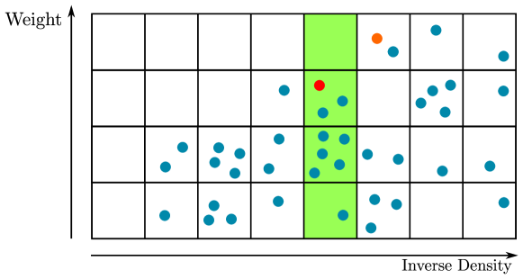
This figure shows a possible state of the algorithm, visualized as a table of weight classes and inverse density classes. Each job appears as a point inside the appropriate entry in the table. The algorithm chooses the maximum weight class of a living job – one such maximum weight job is shown in orange. The algorithm then chooses the minimum ei-density class (i.e. maximum density) in which the total weight of jobs is at least the weight of that orange job – that chosen ei-density class is colored green. Finally, the algorithm chooses a maximum weight job inside the green ei-density class for processing, and this job is shown in red.

Figure 1: The State and Operation of Algorithm 1

1

2Event Function Process() // at any point in time $t$

3       Let $i$ be the largest weight class in which a job is alive.

4      Let $j$ be the minimal ei-density class such that $W_{\top,=j}\left(t\right)\geq u_{i}$.

5      Let $i^{\prime}$ be the maximum weight class in which a job is alive in $Q_{\top,=j}\left(t\right)$.

6      Process a job from $Q_{=i^{\prime},=j}\left(t\right)$ (preferring a partial job if exists).

7

Algorithm 1 Scheduling with Predictions – Weighted

3.2 Analysis

Consider an instance in which the distortion parameter is at most $\mu$. Observe that the ratio between the maximum predicted processing time and the minimum predicted processing time is at most $\mu P$.

Fixing any weight $u_{i}$, observe that a job of weight $u_{i}$ can only belong to ei-density classes in a limited range, which contains at most $\left\lceil\log(\mu P)\right\rceil+1$ classes. We henceforth define $\Lambda:=\left\lceil\log(\mu P)\right\rceil+1$, the maximum number of ei-density classes to which jobs of a specific weight can belong.

The main lemma used to prove Theorem 3.1 is the following, which states that the algorithm is locally competitive.

Lemma 3.4.

At any point in time $t$, it holds that $W\left(t\right)\leq O(\Lambda\mu^{2})\cdot W^{*}\left(t\right)$.

The main focus henceforth would be on proving Lemma 3.4.

Definition 3.5 (analogue of Definition 3.3 for $\operatorname{OPT}$).

For every two predicates $p_{1},p_{2}$ we define

$$Q^{*}_{p_{1},p_{2}}\left(t\right)=\left\{q\in Q^{*}\left(t\right)\middle|p_{1}(\operatorname{wc}\left(q\right))\text{ and }p_{2}(\operatorname{idc}\left(q\right))\right\}$$

We define $W^{*}_{p_{1},p_{2}}\left(t\right)=w(Q^{*}_{p_{1},p_{2}}\left(t\right))$ and $V^{*}_{p_{1},p_{2}}\left(t\right)=y^{*}(Q^{*}_{p_{1},p_{2}}\left(t\right),t)$.

In addition, we use $\Delta$ to denote to volume difference between the algorithm and the optimal solution; for example, $\Delta V_{\leq i,=j}\left(t\right)=V_{\leq i,=j}\left(t\right)-V^{*}_{\leq i,=j}\left(t\right)$.

Definition 3.6 (important weight classes).

We define the following:

1. We define $\operatorname{cwc}\left(t\right)$ to be the weight class of the job processed by the algorithm at time $t$.

2. We define $\operatorname{clw}\left(t\right)$ to be the largest weight class of a living job in the algorithm at $t$.

3. We define $i^{*}\left(t\right)$ to be the minimum weight class such that $u_{i^{*}\left(t\right)}>\frac{4\mu}{\lambda}\cdot W^{*}\left(t\right)$.

The following observation is immediate from the above definition.

Observation 3.7.

There is no job of weight class more than $i^{*}\left(t\right)$ alive in $\operatorname{OPT}$ at time $t$.

Henceforth, fix a point in time $t$ for proving Lemma 3.4. For brevity, we also write $i^{*}$ instead of $i^{*}\left(t\right)$.

The following lemma allows converting weight to volume, and its proof appears in Appendix A.

Lemma 3.8.

Let $i$ be a weight class, and let $j_{1},j_{2}$ be two ei-density classes such that $j_{1}\leq j_{2}$. Then

$$\sum_{j=j_{1}}^{j_{2}}W_{\leq i,=j}\left(t\right)\leq\min\left\{2(j_{2}-j_{1}+1),4\Lambda\right\}\cdot u_{i}+2\mu W^{*}\left(t\right)+2\sum_{j=j_{1}}^{j_{2}}\max\left\{0,\frac{\Delta V_{\leq i,\leq j}\left(t\right)missing}{2^{j}}\right\}$$

Definition 3.9.

Define $t_{j}$ to be the last time prior to $t$ in which the algorithm processed a job of weight class at most $i^{*}$ and ei-density class strictly more than $j$.

Proposition 3.10 shows that the algorithm has low maximum weight at $t_{j}$ for every $j$, and bounds differences in volume between the algorithm and the optimal solution (which enables use of Lemma 3.8). The proof of Proposition 3.10 is given in Appendix A.

Proposition 3.10.

Let $j$ be an ei-density class, then it holds that:

1. $\operatorname{clw}\left(t_{j}\right)\leq i^{*}$

2. $\Delta V_{\leq i^{*},\leq j}\left(t\right)\leq\mu\cdot 2^{j+2}u_{\operatorname{clw}\left(t_{j}\right)}$

Proof of Lemma 3.4.

First, we claim that $\operatorname{clw}\left(t\right)\leq i^{*}$. Assume otherwise, and observe the last time $t^{\prime}$ in which the algorithm processed a job of weight at most $i^{*}$. It must be that $\operatorname{clw}\left(t^{\prime}\right)>i^{*}$; this is since the optimal solution has no jobs of weight class more than $i^{*}$ alive at $t$, and since the algorithm works only on such jobs from $t^{\prime}$ onwards. However, $t^{\prime}$ is also equal to $t_{j}$ for some $j$, which contradicts Proposition 3.10. Thus, it must be that $\operatorname{clw}\left(t\right)\leq i^{*}$.

Let $j_{\min}$ be the minimum ei-density class in which a job of weight class at most $i^{*}$ can exist, and let $j_{\max}$ be the maximum possible ei-density class. It holds that

$$W\left(t\right) =\sum_{j=j_{\min}}^{j_{\max}}W_{\leq i^{*},=j}\left(t\right)$$

$$\leq 4\Lambda u_{i^{*}}+2\mu W^{*}\left(t\right)+\sum_{j=j_{\min}}^{j_{\max}}2\max\left\{0,\frac{\Delta V_{\leq i^{*},\leq j}\left(t\right)missing}{2^{j}}\right\}$$

$$\leq 4\Lambda u_{i^{*}}+2\mu W^{*}\left(t\right)+\sum_{j=j_{\min}}^{j_{\max}}8\mu\cdot u_{\operatorname{clw}\left(t_{j}\right)}$$

where the equality is due to $\operatorname{clw}\left(t\right)\leq i^{*}$, the first inequality is due to Lemma 3.8 and the second inequality follows from Proposition 3.10. Now, consider that for every ei-density class $j$, at $t_{j}$ we processed a job $q$ of ei-density class $h$ where $h>j$, such that $\operatorname{wc}\left(q\right)\leq\operatorname{clw}\left(t_{j}\right)$. There also existed at $t_{j}$ a job $q^{\prime}$ such that $\operatorname{wc}\left(q^{\prime}\right)=\operatorname{clw}\left(t_{j}\right)$; denote its ei-density class $h^{\prime}:=\operatorname{idc}\left(q^{\prime}\right)$. It holds that $h^{\prime}\geq h$, otherwise $q^{\prime}$ would have been chosen for processing at $t_{j}$ instead of $q$. Thus, it must be the case that an ei-density class larger than $j$ is one of the $\Lambda$ ei-density classes to which $\operatorname{clw}\left(t_{j}\right)$ can belong.

From the preceding argument, $i^{*}=\operatorname{clw}\left(t_{j}\right)$ can hold for at most $\Lambda$ values of $j$; $i^{*}-1=\operatorname{clw}\left(t_{j}\right)$ can hold for at most $\Lambda$ additional values of $j$; and so on. It thus holds that:

$$8\mu\sum_{j=j_{\min}}^{j_{\max}}u_{\operatorname{clw}\left(t_{j}\right)}\leq 8\mu\Lambda\sum_{k=0}^{\infty}u_{i^{*}-k}\leq 16\mu\Lambda u_{i^{*}}$$

Therefore, we have

$$W\left(t\right)\leq\Lambda(16\mu+4)u_{i^{*}}+2\mu W^{*}\left(t\right)$$ (1)

Observe that $u_{i^{*}}\leq 4\mu W^{*}\left(t\right)$ – this stems from the definition of $i^{*}$. Plugging into Equation 1, we get that

$$W\left(t\right)\leq O(\Lambda\mu^{2})W^{*}\left(t\right)\qed$$

Proof of Theorem 3.1.

Plugging the definition of $\Lambda$ into Lemma 3.4, we have that

$$W\left(t\right)\leq O(\mu^{2}\log(\mu P))W^{*}\left(t\right)$$

Recall that this is after the rounding of the weights to powers of $\lambda=\Theta(\mu)$; taking this rounding into account, the algorithm is $O(\mu^{3}\log(\mu P))$-competitive. ∎

3.3 Ratio of Densities

Recall that the density of a job $q$ is $\frac{w_{q}}{p_{q}}$. We show that the dependence on $P$ in the competitiveness of Algorithm 1 (as stated in Theorem 3.1) can be replaced with a dependence on the parameter $D$, which is the maximum ratio of the densities of two jobs in the input. Concretely, we show that the following theorem holds.

Theorem 3.11.

Algorithm 1 is a $\mu$-robust, $O(\mu^{3}\log(\mu D))$-competitive algorithm for the sppt problem.

The proof of Theorem 3.11 appears in Appendix E, and is almost immediate from the previous proof of Theorem 3.1.

4 Weighted Flow Time – Ratio of Weights

In this section, we present the $O(\mu^{2}\log W)$-competitive $\mu$-robust algorithm for sppt with weighted flow time. We do so in two steps: first, we introduce $\mu$-robust algorithm for the unweighted setting, which is $2\left\lceil{\mu}^{2}\right\rceil$-competitive. Then, we show that instances of this unweighted algorithm can be combined and applied to the weighted setting, at an additional loss of an $O(\log W)$ factor in competitiveness.

4.1 The Algorithm for Unweighted Flow Time in the Prediction Model

In this subsection, we present an algorithm in the prediction model for the unweighted setting – that is, where $w_{q}=1$ for all $q\in Q$.

4.1.1 The Algorithm

The algorithm holds each pending job in one of two bins, a “full” bin $F$ and a “partial” bin $P$. The algorithm attempts to divide the total weight of the pending jobs equally between the two bins. The algorithm refers to the pending jobs in $F$ by $Q_{F}$ and the pending jobs in $P$ by $Q_{P}$. For ease of notation, we also define $\delta_{F}=\left|Q_{F}\right|$ and $\delta_{P}=\left|Q_{P}\right|$.

The course a job undergoes in the algorithm consists of being initially assigned to bin $F$, then moving to bin $P$, and finally being processed in bin $P$ until its eventual completion. The algorithm maintains a bijective priority mapping $\pi_{F}:Q_{F}\to\left\{1,2,\cdots,\delta_{F}\right\}$ from the living jobs $Q_{F}$ to the natural integers from $1$ to $\delta_{F}$. This mapping determines the priority of the jobs of $F$. That is, whenever moving a job from $F$ to $P$ is required, the algorithm moves the highest priority job ($q$ such that $\pi_{F}(q)=\delta_{F}$).

The algorithm also maintains (implicitly) a priority mapping $\pi_{P}:Q_{P}\to\left\{1,2,\cdots,\delta_{P}\right\}$, such that the highest priority job is chosen to be processed. This priority mapping is simply LIFO according to the time in which the job moved from $F$ to $P$.

Definition 4.1 (violation).

Observe two jobs $q_{1},q_{2}\in Q_{F}$ in the algorithm. We say that the ordered pair $(q_{1},q_{2})$ is a violation if $\pi_{F}(q_{1})>\pi_{F}(q_{2})$ and $\mu\cdot\tilde{p}_{q_{2}}\leq\tilde{p}_{q_{1}}$. Informally, the algorithm assigns priority to $q_{1}$ over $q_{2}$ even though it knows that the processing time of $q_{2}$ (which is strictly smaller than $\mu\cdot\tilde{p}_{q_{2}}$) is strictly smaller than that of $q_{1}$.

Algorithm’s Description and Intuition. The algorithm maintains two properties regarding the priorities in the bin $F$. The first property is that there exist no violations. When this holds, the priority is “quasi-SRPT”; that is, if a job has a higher priority than another job, then the lower bound on the processing time of the first job is no more than the upper bound on the processing time of the second job (noting that in $F$ the remaining processing time is equal to the initial processing time). This “quasi-SRPT” property is used in Proposition B.8. The second property is that for every natural $k$, the total processing time of the $k$ lowest priority jobs never decreases upon the release of a new job, which is used in Proposition B.6.

The way in which the algorithm maintains both of those traits for the bin $F$ can be seen in the function UponJobRelease(q), which is called upon the release of a new job $q$. The algorithm first gives the newly-released job the maximum priority in $F$, which does not affect the second property, but could possibly break the first property by causing violations. In order to fix these violations, the algorithm performs a rotation of the new job $q$ and all violations. That is, numbering the jobs in violation with $q$ as $q_{1},\cdots,q_{m}$ by order of decreasing priority, the rotation simultaneously sets the new priority of $q$ to be the old priority of $q_{m}$, the new priority of $q_{m}$ to be the old priority of $q_{m-1}$, and so on (the new priority of $q_{1}$ is the old priority of $q$, i.e. the maximum priority). In Algorithm 2, this rotation operation is described as simply composing the mapping $\pi_{F}$ with the cyclic permutation $\sigma=\left(\pi_{F}(q_{m}),\pi_{F}(q_{m-1}),\cdots,\pi_{F}(q_{1}),\pi_{F}(q)\right)$, where $\sigma$ maps from the natural numbers $\left[\delta_{F}\right]$ to $\left[\delta_{F}\right]$, and is written in cycle notation. In the analysis, we show that this rotation is sufficient to solve any violations that occur in the insertion.

Visualization in Figures.

Visualizations of the state of Algorithm 2 are given throughout the paper (e.g. in Figure 2c). In these visualizations, each job is visualized as a rectangle, where the height of the rectangle is the weight of the job (which is currently $1$, since we’re considering the unweighted setting). The area of the rectangle is the remaining volume of the job. Consider the transformation of the rectangle as a job is processed: its weight (height) remains the same but its volume (area) decreases. Hence, the width of the rectangle decreases as the job is processed.

A bin (either $F$ or $P$) is visualized as a “stack” of the jobs in that bin. Those jobs are stacked according to their priority in the bin (the highest priority job is at the top of the stack). At any point in time, the highest priority job in $P$ is processed – this is the job at the top of the visualization of $P$.

These visualizations are for the sake of understanding the algorithm and its proof, and are not used in the algorithm itself. The algorithm is not aware of the details of the visualization, and in particular is not aware of the volume of the jobs (i.e. the area of the rectangles).

The algorithm is shown in Algorithm 2. Figures 2c and 3 visualize Algorithm 2.

1

2Event Function UponJobRelease($q$) // upon the release of a job $q$ at time $t$

3       Set $Q_{F}\leftarrow Q_{F}\cup\left\{q\right\}$, and set $\pi_{F}(q)\leftarrow\delta_{F}$.

4      // rotate the priorities of jobs to fix violations

5      if there exists $q^{\prime}\in Q_{F}\backslash\left\{q\right\}$ such that $(q,q^{\prime})$ is a violation then

6             let $Q^{\prime}=\left\{q^{\prime}\in Q_{F}\backslash\{q\}\middle|(q,q^{\prime})\text{ is a violation}\right\}$.

7            denoting $m=\left|Q^{\prime}\right|$, let $q_{1},\cdots,q_{m}$ be an enumeration of $Q^{\prime}$ such that $\pi_{F}(q)>\pi_{F}(q_{1})>\cdots>\pi_{F}(q_{m})$.

8            let $\sigma$ be the cyclic permutation $\left(\pi_{F}(q_{m}),\pi_{F}(q_{m-1}),\cdots,\pi_{F}(q_{1}),\pi_{F}(q)\right)$.

9            set $\pi_{F}\leftarrow\sigma\circ\pi_{F}$

10      

11

12Event Function UponHeavyF() // upon $\delta_{F}>\delta_{P}$

13       let $q\in Q_{F}$ be such that $\pi_{F}(q)=\delta_{F}$.

14      move $q$ from $F$ to $P$, and set $\pi_{P}(q)=\delta_{P}$.

15

16Event Function Process() // at any point in time $t$

17       let $q\in Q_{P}$ be such that $\pi_{P}(q)=\delta_{P}$.

18      process $q$.

19

Algorithm 2 Scheduling with Predictions – Unweighted

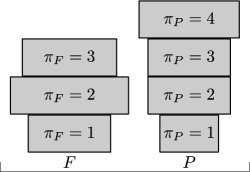
(a)

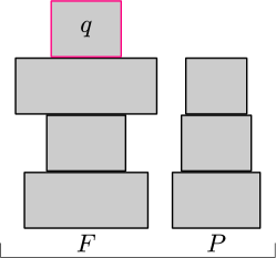
(b)

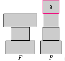
(c)

Figure 2: The State of Bins and UponHeavyF in Algorithm 2

LABEL:subfig:UW_Structure shows a possible state of the algorithm at some point in time. In the figure, the bin $F$ contains $3$ pending jobs, and the bin $P$ contains $4$ pending jobs. In this figure, the job being processed is the job of priority $4$ in $P$.

LABEL:subfig:UW_Transfer1 and LABEL:subfig:UW_Transfer2 show the operation of UponHeavyF. At the state of LABEL:subfig:UW_Transfer1, $\delta_{F}>\delta_{P}$ and so UponHeavyF is called. The top priority job $q$ in $F$ is then moved to $P$ , where it also has top priority (LABEL:subfig:UW_Transfer2).

(a)

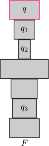
(b)

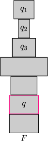
(c)

Figure 3: UponJobRelease in Algorithm 2

The competitiveness guarantee of Algorithm 2 is given in Theorem 4.2, the proof of which is given in Subsection B.1.

Theorem 4.2.

Algorithm 2 is a $\mu$-robust, $2\left\lceil\mu^{2}\right\rceil$-competitive algorithm for the unweighted sppt problem.

4.2 The $O(\mu^{2}\log W)$-competitive Algorithm for Weighted Flow Time

Having described the unweighted algorithm in the previous subsections, we present the $O(\mu^{2}\log W)$-competitive algorithm for the weighted setting.

4.3 The Algorithm

We assume that the weights of incoming jobs are of an integer power of $2$; the algorithm can enforce this by rounding weights, incurring a factor of at most $2$ to its competitive ratio.

For each $i\in\mathbb{Z}$, the algorithm maintains a superbin $A^{i}$ (only nonempty superbins are maintained explicitly). The superbin is constructed as in Subsection 4.1. That is, $A^{i}$ contains two bins $F^{i}$ and $P^{i}$ (containing the pending jobs $Q_{F^{i}}$ and $Q_{P^{i}}$, respectively), and maintains the priority bijections $\pi_{F^{i}}$ and $\pi_{P^{i}}$ on the jobs of $F^{i}$ and $P^{i}$, respectively. As in the weighted case, the algorithm refers to $\left|Q_{F^{i}}\right|$ and $\left|Q_{P^{i}}\right|$ by $\delta_{F^{i}}$ and $\delta_{P^{i}}$, respectively.

The algorithm sends released jobs of weight $2^{i}$ (for any $i\in\mathbb{Z}$) to the superbin $A^{i}$. The insertion to the superbin $A^{i}$ is according to UponJobRelease in Algorithm 2. That is, the released job $q$ is first inserted to $F^{i}$, the algorithm sets $\pi_{F^{i}}(q)\leftarrow\delta_{F^{i}}$, and then possibly performs a rotation to solve violations. For every superbin index $i$, the algorithm also maintains that $w(Q_{F^{i}})\leq w(Q_{P^{i}})$, by moving jobs from $F^{i}$ to $P^{i}$ as in Subsection 4.1, performed by calling UponHeavyF as defined in Algorithm 2.

As for processing, the algorithm chooses for processing the superbin $A^{i}$ with the heaviest partial bin $P^{i}$. When a superbin $A^{i}$ is chosen for processing, algorithm makes a call to Process as defined in Algorithm 2, which chooses the job $q\in Q_{P^{i}}$ such that $\pi_{P^{i}}(q)$ is maximal.

The algorithm is given in Algorithm 3. A possible state of Algorithm 3 is visualized in Figure 4.

1

2Event Function UponJobRelease($q$) // upon the release of a job $q$ at time $t$

3      

4      let $i$ be such that $w_{q}=2^{i}$.

5      call $A^{i}.\textnormal{{\sc UponJobRelease(}}\textnormal{\emph{q}}\textnormal{{\sc)}}$

6

7Event Function Process() // at any point in time $t$

8       let $i=\arg\max_{i^{\prime}}w(P^{i^{\prime}})$.

9      call $A^{i}.\textnormal{{\sc Process(}}\textnormal{\emph{}}\textnormal{{\sc)}}$.

10

11Event Function UponHeavyF($i$) // upon $w(F^{i})>w(P^{i})$ for some index $i$

12       call $A^{i}.\textnormal{{\sc UponHeavyF(}}\textnormal{\emph{}}\textnormal{{\sc)}}$

13

Algorithm 3 Scheduling with Predictions – $O(\log W)$-Competitive

Figure 4: A Possible State of Algorithm 3

The competitiveness guarantee of Algorithm 3 is given in Theorem 4.3, the proof of which appears in Subsection B.2.

Theorem 4.3.

Algorithm 3 is a $\mu$-robust, $O\left(\mu^{2}\log W\right)$-competitive algorithm for the sppt problem.

5 Discussion and Open Problems

This paper presents algorithms for sppt for minimizing weighted flow time which have a polynomial dependency on the distortion $\mu$ of the given predictions, such that when this distortion is constant the best known competitiveness bounds are matched (namely, $O(\log P)$, $O(\log D)$ and $O(\log W)$). These are the first algorithms to maintain any nontrivial competitiveness when given inaccurate processing times in the weighted flow time setting.

However, in the model which we consider, each such $\mu$-robust algorithm is tailored to a specific value of $\mu$. One could desire an algorithm which works for any $\mu$, while maintaining a competitive ratio which is a function of this $\mu$. In many other problems, going from the first model to the second model can be very easily done through a doubling procedure on the parameter $\mu$; however, applying such a doubling scheme to this scheduling problem does not seem immediate, and we leave its development to future work.

The dependencies of our algorithms on the maximum distortion are $O(\mu^{2})$ and $\tilde{O}(\mu^{3})$. Improving the dependence on $\mu$ in the competitiveness is also an interesting problem; we conjecture that a linear dependence on $\mu$ is the optimal one.

Another problem is determining the exact competitive ratio for $\mu$-robust algorithm as $\mu$ approaches $1$ (i.e. small distortion). This problem is most salient for unweighted flow time, in which we’ve shown a lower bound of $2$-competitiveness, and our upper bound result only yields $4$-competitiveness.

Appendix A Additional proofs from Section 3

Proof of Lemma 3.8.

Observe that $\sum_{j=j_{1}}^{j_{2}}W_{\leq i,=j}\left(t\right)=\sum_{j=j_{1}}^{j_{2}}W^{\textrm{p}}_{\leq i,=j}\left(t\right)+\sum_{j=j_{1}}^{j_{2}}W^{\textrm{f}}_{\leq i,=j}\left(t\right)$, where the superscripts p and f refer to partial and full jobs, respectively.

The algorithm maintains that in every weight class + ei-density class combination, there exists at most one partial job of those classes. Thus, for every ei-density class $j$, a geometric sum yields that $W^{\textrm{p}}_{\leq i,=j}\left(t\right)\leq 2w^{j}$, where $w^{j}$ is the maximum weight of a partial job in $Q_{\leq i,=j}\left(t\right)$. Since $w^{j}\leq u_{i}$, we thus have that $W^{\textrm{p}}_{\leq i,=j}\left(t\right)\leq 2u_{i}$, and thus $\sum_{j=j_{1}}^{j_{2}}W^{\textrm{p}}_{\leq i,=j}\left(t\right)\leq 2(j_{2}-j_{1}+1)u_{i}$. In addition, each weight class can exist in at most $\Lambda$ different ei-density classes, which yields

$$\sum_{j=j_{1}}^{j_{2}}W^{\textrm{p}}_{\leq i,=j}\left(t\right)\leq\sum_{j=j_{1}}^{j_{2}}2w^{j}\leq 2u_{i}\Lambda+2u_{i-1}\Lambda+\cdots\leq 4u_{i}\Lambda$$

Combining, we have $\sum_{j=j_{1}}^{j_{2}}W^{\textrm{p}}_{\leq i,=j}\left(t\right)\leq\min\left\{2(j_{2}-j_{1}+1),4\Lambda\right\}\cdot u_{i}$.

It remains to bound the weight of the full jobs, namely $\sum_{j=j_{1}}^{j_{2}}W^{\textrm{f}}_{\leq i,=j}\left(t\right)$.

$$\sum_{j=j_{1}}^{j_{2}}W^{\textrm{f}}_{\leq i,=j}\left(t\right) \leq\sum_{j=j_{1}}^{j_{2}}\frac{V_{\leq i,=j}\left(t\right)missing}{2^{j}}$$

$$\leq\sum_{j=j_{1}}^{j_{2}}\frac{\Delta V_{\leq i,=j}\left(t\right)+V^{*}_{\leq i,=j}\left(t\right)missing}{2^{j}}$$

$$\leq 2\mu\sum_{j=j_{1}}^{j_{2}}W^{*}_{\leq i,=j}\left(t\right)+\sum_{j=j_{1}}^{j_{2}}\frac{\Delta V_{\leq i,\leq j}\left(t\right)-\Delta V_{\leq i,\leq j-1}\left(t\right)missing}{2^{j}}$$

$$\leq 2\mu\sum_{j=j_{1}}^{j_{2}}W^{*}_{\leq i,=j}\left(t\right)+\frac{\Delta V_{\leq i,\leq j_{2}}\left(t\right)missing}{2^{j_{2}}}+\sum_{j=j_{1}}^{j_{2}-1}\frac{\Delta V_{\leq i,\leq j}\left(t\right)missing}{2^{j+1}}-\frac{\Delta V_{\leq i,\leq j_{1}-1}\left(t\right)missing}{2^{j_{1}}}$$

$$\leq 2\mu\sum_{j=j_{1}}^{j_{2}}W^{*}_{\leq i,=j}\left(t\right)+\frac{\Delta V_{\leq i,\leq j_{2}}\left(t\right)missing}{2^{j_{2}}}+\sum_{j=j_{1}}^{j_{2}-1}\frac{\Delta V_{\leq i,\leq j}\left(t\right)missing}{2^{j+1}}+\mu W^{*}_{\leq i,\leq j_{1}-1}\left(t\right)$$

$$\leq 2\mu\sum_{j=j_{1}}^{j_{2}}W^{*}_{\leq i,=j}\left(t\right)+\sum_{j=j_{1}}^{j_{2}}\max\left\{0,\frac{\Delta V_{\leq i,\leq j}\left(t\right)missing}{2^{j}}\right\}+\mu W^{*}_{\leq i,\leq j_{1}-1}\left(t\right)$$

$$\leq 2\mu W^{*}_{\leq i,\leq j_{2}}\left(t\right)+\sum_{j=j_{1}}^{j_{2}}\max\left\{0,\frac{\Delta V_{\leq i,\leq j}\left(t\right)missing}{2^{j}}\right\}$$

$$\leq 2\mu W^{*}\left(t\right)+\sum_{j=j_{1}}^{j_{2}}\max\left\{0,\frac{\Delta V_{\leq i,\leq j}\left(t\right)missing}{2^{j}}\right\}$$

where the first inequality is due to the fact that a full job $q$ of ei-density class $j$ has at least $w_{q}\cdot 2^{j}$ remaining volume, the second and fifth inequalities are due to the fact that every job $q$ of ei-density class at most $j$ in the optimal solution has at most $2^{j+1}\mu w_{q}$ volume. ∎

Proof of Proposition 3.10.

First, we show that for every $j$, the first claim implies the second claim. Then, we prove the first claim by induction on the ei-density classes, in decreasing order. Combining these two proofs, the proposition holds.

The first claim implies the second claim. Assume that $\operatorname{clw}\left(t_{j}\right)\leq i^{*}$ for some $j$. Since the optimal solution has no jobs of weight more than $u_{i^{*}}$ alive at time $t$, and since the algorithm did have any such jobs alive at $t_{j}$, it must be that the algorithm worked on such jobs during $\left[t_{j},t\right)$ at least as much as the optimal solution. In addition, the algorithm did not work on any jobs of weight at most $u_{i^{*}}$ and ei-density class more than $j$ during this interval. Thus, it holds that

$$\Delta V_{\leq i^{*},\leq j}\left(t\right)\leq\Delta V_{\leq i^{*},\leq j}\left(t_{j}\right)\leq V_{\leq i^{*},\leq j}\left(t_{j}\right)$$

Thus, it’s enough to bound $V_{\leq i^{*},\leq j}\left(t_{j}\right)$. Observe that since the algorithm chose to process a job of ei-density class more than $j$, the total weight in each ei-density class $j^{\prime}\leq j$ is at most $\operatorname{clw}\left(t_{j}\right)$. Thus, the total volume at $t_{j}$ in ei-density class $j^{\prime}$ is at most $\mu\cdot 2^{j^{\prime}+1}u_{\operatorname{clw}\left(t_{j}\right)}$. Summing over all $j^{\prime}\leq j$ yields a geometric sum, which is at most $2^{j+2}u_{\operatorname{clw}\left(t_{j}\right)}$, showing that the first claim indeed implies the second claim.

The first claim holds. We prove the first claim of the proposition by induction on the ei-density classes, in decreasing order. For the base case of the largest ei-density class $j_{\max}$, we have $t_{j_{\max}}=0$ and thus the claim holds.

Now, let $j$ be any ei-density class and suppose that the claim holds for all ei-density classes $j+1$ and above. Assume for contradiction that $\operatorname{clw}\left(t_{j}\right)>i^{*}$. Let $q$ be the job chosen for processing at $t_{j}$, and define $h:=\operatorname{idc}\left(q\right)$. From the definition of $t_{j}$, we know that $\operatorname{wc}\left(q\right)\leq i^{*}$ and that $h>j$.

Since the algorithm always processes the maximum-weight job in the chosen ei-density class, we know that

$$W_{\leq\operatorname{wc}\left(q\right),=h}\left(t_{j}\right)=W_{\top,=h}\left(t_{j}\right)\geq u_{\operatorname{clw}\left(t_{j}\right)}$$

where the inequality is due to the choice of the algorithm.

Now, since during $\left[t_{j},t\right)$ the algorithm did not process any jobs of weight class at most $i^{*}$ and ei-density class more than $j$, it must be that

$$W_{\leq i^{*},=h}\left(t\right)\geq W_{\leq i^{*},=h}\left(t_{j}\right)=W_{\leq\operatorname{wc}\left(q\right),=h}\left(t\right)\geq u_{\operatorname{clw}\left(t_{j}\right)}-u_{i^{*}}$$

where the minus term is due to the fact that the algorithm could have completed $q$ exactly at $t_{j}$.

Now, using Lemma 3.8, we have

$$W_{\leq i^{*},=h}\left(t\right) \leq 2\cdot u_{i^{*}}+2\mu W^{*}\left(t\right)+2\max\left\{0,\frac{\Delta V_{\leq i^{*},\leq h}\left(t\right)}{2^{h}}\right\}$$

$$\leq 2\cdot u_{i^{*}}+2\mu W^{*}\left(t\right)+8\mu u_{\operatorname{clw}\left(t_{h}\right)}$$

$$\leq 2\cdot u_{i^{*}}+2\mu W^{*}\left(t\right)+8\mu u_{i^{*}}$$

$$=(8\mu+2)u_{i^{*}}+2\mu W^{*}\left(t\right)$$

where the second inequality uses the induction hypothesis that the first claim holds for $h$, combined with the previous proof that the first claim implies the second claim. The third inequality also uses the induction hypothesis.

Combining, we have $2\mu W^{*}\left(t\right)\geq u_{\operatorname{clw}\left(t_{j}\right)}-(8\mu+3)u_{i^{*}}\geq u_{i^{*}+1}-(8\mu+3)u_{i^{*}}=\frac{\lambda}{2}\cdot u_{i^{*}}$. Thus, we get that $W^{*}\left(t\right)\geq\frac{\lambda}{4\mu}\cdot u_{i^{*}}$, in contradiction to the definition of $i^{*}$. This proves the first claim of the proposition. ∎

Appendix B Additional proofs from Section 4

B.1 Proof of Theorem 4.2

In the following analysis, we prove Theorem 4.2.

Definition B.1.

For every time $t$, we define $Q_{F}(t)$ and $Q_{P}(t)$ to be the values of the variables $Q_{F}$ and $Q_{P}$ at time $t$. We also define $Q(t)$ to be the set of jobs pending in the algorithm at time $t$, where it holds that $Q(t)=Q_{F}(t)\cup Q_{P}(t)$.

In addition, we use $\delta(t),\delta_{F}(t),\delta_{P}(t)$ to denote the cardinalities of $Q(t),Q_{F}(t),Q_{P}(t)$ respectively.

We also use $\pi_{F}^{t}$ and $\pi_{P}^{t}$ to denote the values of $\pi_{F}$ and $\pi_{P}$ at time $t$, respectively.

Definition B.2.

For every time $t$ and job $q\in Q_{F}(t)$, define $X(q,t)=\left\{q^{\prime}\in Q_{F}(t)\middle|\pi_{F}(q^{\prime})\leq\pi_{F}(q)\right\}$. For ease of notation, we denote $w(X(q,t))$ by $\beta(q,t)$. We also similarly define $X(q,t)$ and $\beta(q,t)$ for $q\in Q_{P}(t)$ according to $\pi_{P}$.

Definition B.3 (volume of job covered by bar).

For any $x\in\mathbb{R}^{+}\cup\left\{0\right\}$ and time $t$, and for any job $q\in Q(t)$, we define

$$\gamma_{q}(x,t)=\begin{cases}y_{q}(t)&x\geq\beta(q,t)\\ 0&\text{otherwise}\end{cases}$$

called the volume of $q$ covered by $x$ at $t$.

Definition B.4 (volume covered by bar).

We define:

1. The covered volume of $x$ at $t$, which is $B\left(x,t\right)=\sum_{q\in Q(t)}\gamma_{q}(x,t)$.

2. $B_{F}\left(x,t\right)=\sum_{q\in Q_{F}(t)}\gamma_{q}(x,t)$.

3. $B_{P}\left(x,t\right)=\sum_{q\in Q_{P}(t)}\gamma_{q}(x,t)$.

Observe that $B\left(x,t\right)=B_{F}\left(x,t\right)+B_{P}\left(x,t\right)$

This figure shows the state of the algorithm at some time $t$, and visualizes the volume covered by a bar $x\in\mathbb{R}^{+}\cup\left\{0\right\}$ at $t$. Here, for each job $q$ we have that $\gamma_{q}(x,t)$ is the orange-colored area of the job (which is either $0$ or $y_{q}(t)$). Thus, the total covered volume $B\left(x,t\right)$ is the total orange-colored area in the figure.

Figure 5: Volume Covered by Bar

In the following analysis we consider various properties of the functions of our algorithm. When considering a function call at time $t$, we use $t^{-}$ to denote the time immediately before the function call, and use $t$ to denote the time immediately after the function call.

Proposition B.5.

Let $t$ be any time in which UponHeavyF is called. Then for every $x\in\mathbb{R}^{+}\cup\left\{0\right\}$ we have that

$$B\left(x,t\right)=B\left(x,t^{-}\right)$$

Proof.

Let $q$ be the job moved from $F$ to $P$. It holds that $\pi_{F}^{t^{-}}(q)=\delta_{F}(t^{-})$ and that $\pi_{P}^{t}(q)=\delta_{P}(t)$. Thus, we have that for every job $q^{\prime}\in Q(t)\backslash\{q\}$ it holds that $\beta(q^{\prime},t)=\beta(q^{\prime},t^{-})$, and thus an identical amount of the volume of $q^{\prime}$ is covered by $x$ at $t^{-}$ and at $t$.

As for the volume of $q$, it holds that $\beta(q,t^{-})=\delta_{F}(t^{-})$. Now observe that $\delta_{F}(t^{-})=\delta_{P}(t^{-})+1$, since UponHeavyF was called (it cannot be that $\delta_{F}(t^{-})>\delta_{P}(t^{-})+1$, since an earlier call to UponHeavyF would fix this imbalance). Thus, after moving $q$ we have that $\delta_{P}(t)=\delta_{F}(t^{-})$. We therefore have that

$$\beta(q,t)=\delta_{P}(t)=\delta_{F}(t^{-})=\beta(q,t^{-})$$

Overall, we have that $\beta(q^{\prime},t^{-})=\beta(q^{\prime},t)$ for every $q^{\prime}\in Q(t)$, and thus $B\left(x,t\right)=B\left(x,t^{-}\right)$, as required. ∎

Proposition B.6.

Consider a call to UponJobRelease(q) at time $t$. For every $x\in\mathbb{R}^{+}\cup\left\{0\right\}$, it holds that

$$B\left(x,t\right)\geq B\left(x,t^{-}\right)$$

Proof.

We denote by $t_{0}$ the “time” immediately after adding $q$ to $\pi_{F}$ – that is, the state of the algorithm before Algorithm 2 in $\textnormal{{\sc UponJobRelease}}(q)$.

Claim 1: $B\left(x,t_{0}\right)\geq B\left(x,t^{-}\right)$. Since $\pi_{F}^{t_{0}}(q)=\delta_{F}(t_{0})$, we have that $\pi_{F}^{t_{0}}(q)>\pi_{F}^{t_{0}}(q^{\prime})$ for every $q^{\prime}\in Q_{F}(t^{-})$. For every such $q^{\prime}$ we thus have $\beta(q^{\prime},t_{0})=\beta(q^{\prime},t^{-})$, and therefore $B\left(x,t_{0}\right)\geq B\left(x,t^{-}\right)$.

Claim 2: $B\left(x,t\right)\geq B\left(x,t_{0}\right)$. If no violations exist at $t_{0}$, and thus no rotation is performed, then the claim holds. Otherwise, the cyclic permutation $\left(\pi_{F}(q_{m}),\pi_{F}(q_{m-1}),\cdots,\pi_{F}(q_{1}),\pi_{F}(q)\right)$ is applied, where the jobs $q_{1},\cdots,q_{m}$ are the jobs involved in violations with $q$ at $t_{0}$, such that $\pi_{F}^{t_{0}}(q_{i})>\pi_{F}^{t_{0}}(q_{i-1})$ for every $i>0$.

We write $q_{0}=q$, and observe the set of jobs $Q^{\prime}=\left\{q_{0},q_{1},\cdots q_{m}\right\}$ involved in the cyclic permutation. Since the only change is in priorities between $t$ and $t_{0}$ is in $Q^{\prime}$, it remains to observe the change in the volume of $Q^{\prime}$ covered by $x$. If $\pi_{F}^{t_{0}}(q^{\prime})>x$ for every $q^{\prime}\in Q^{\prime}$, the volume of $Q^{\prime}$ covered by $x$ does not change. The same holds if $\pi_{F}^{t_{0}}(q^{\prime})\leq x$ for every $q^{\prime}\in Q^{\prime}$.

It remains to observe the case in which $x$ covers some of $Q^{\prime}$ but not all. In this case, let $i$ be the smallest index such that $\pi_{F}^{t_{0}}(q_{i})\leq x$, such that $i>0$. After applying the cyclic permutation, we have that the volume covered by $x$ has decreased by $p_{q_{i}}$ (since $\pi_{F}^{t}(q_{i})=\pi_{F}^{t_{0}}(q_{i-1})$), but has increased by $p_{q_{0}}$ (since $\pi_{F}^{t}(q_{0})=\pi_{F}^{t_{0}}(q_{m})$). Now, recall that $q_{0}=q$, and that $(q,q_{i})$ was a violation at $t_{0}$. This implies that

$$p_{q_{i}}<\mu\tilde{p}_{q_{i}}\leq\tilde{p}_{q}\leq p_{q}$$

proving the second claim.

Combining the two claims, we have that

$$B\left(x,t\right)\geq B\left(x,t^{-}\right)$$

as required. ∎

Proposition B.7.

Outside of function calls, there are no violations in the algorithm.

Proof.

Observe that the only changes to $F$ occur in calls to UponJobRelease and UponHeavyF. We show that if there is no violation before such a function call, then there would be no violation after the function call.

In the case of UponHeavyF, this trivially holds, since removing a job from $F$ cannot cause a new violation. It remains to consider UponJobRelease.

Suppose that UponJobRelease(q) is called at time $t$. As in the proof of Proposition B.6, we denote by $t_{0}$ the time immediately after the insertion of the job $q$ into $F$, and before the possible rotation of Algorithm 2. By the induction hypothesis, and through the fact that $\pi_{F}^{t_{0}}(q)=\delta_{F}(t_{0})$, the only violations at $t_{0}$ are of the form $(q,q^{\prime})$ for some $q^{\prime}\in Q_{F}(t_{0})\backslash\{q\}$. If there are no such violations then no rotation occurs, and thus the state at time $t$ contains no violations, completing the proof.

Otherwise, denoting $q_{0}=q$, the set $Q^{\prime}=\{q_{0},q_{1},\cdots,q_{m}\}$ is rotated. For ease of notation, we write $Q^{\prime\prime}=Q_{F}(t_{0})\backslash Q^{\prime}$. Consider the possible violations at time $t$, after this rotation.

1. violations of the form $(q^{\prime\prime}_{1},q^{\prime\prime}_{2})$ for some $q^{\prime\prime}_{1},q^{\prime\prime}_{2}\in Q^{\prime\prime}$. Such violations cannot occur in $t$, since they did not exist in $t_{0}$, and since $\pi_{F}^{t}(q^{\prime\prime})=\pi_{F}^{t_{0}}(q^{\prime\prime})$ for every $q^{\prime\prime}\in Q^{\prime\prime}$.

2. violations between $q_{i}$ and $q^{\prime\prime}$ for some index $0<i\leq m$ and some job $q^{\prime\prime}\in Q^{\prime\prime}$. Consider that there was no violation between $q_{i}$ and $q^{\prime\prime}$ at time $t_{0}$. Since $\pi_{F}^{t}(q^{\prime\prime})=\pi_{F}^{t_{0}}(q^{\prime\prime})$, and since $\pi_{F}^{t}(q_{i})\geq\pi_{F}^{t_{0}}(q_{i})$, it must be that the violation is of the form $(q_{i},q^{\prime\prime})$.

   Now, observe that $\pi_{F}^{t}(q_{i})\leq\pi_{F}^{t}(q)$. In addition, since $(q,q_{i})$ was a violation at $t_{0}$, it holds that $\tilde{p}_{q_{i}}<\mu\tilde{p}_{q_{i}}\leq\tilde{p}_{q}$. Thus, if $(q_{i},q^{\prime\prime})$ is a violation at $t$, it must be that $(q,q^{\prime\prime})$ was a violation at $t_{0}$, in contradiction to $q^{\prime\prime}\in Q^{\prime\prime}$.

3. violations of the form $(q_{i},q_{j})$ for $1\leq i,j\leq m$. Observe that there was no violation between $q_{i}$ and $q_{j}$ at time $t_{0}$, and that the order between their priorities did not change between $t_{0}$ and $t$. Thus, there is no violation between them at $t$.

4. violations between $q_{i}$ and $q$, for some index $i$. Consider that since $\pi_{F}^{t}(q)\leq\pi_{F}^{t}(q_{i})$, the violation must be of the form $(q_{i},q)$. Now, consider that $(q,q_{i})$ was a violation at $t_{0}$, and thus $\mu\tilde{p}_{q}>\tilde{p}_{q}\geq(1+\epsilon_{q_{i}})\tilde{p}_{q_{i}}>\tilde{p}_{q_{i}}$. Thus, $(q_{i},q)$ cannot be a violation at $t$.

5. violations between $q$ and $q^{\prime\prime}$, for some $q^{\prime\prime}\in Q^{\prime\prime}$. Since $(q,q^{\prime\prime})$ was not a violation at $t_{0}$, and since $\pi_{F}^{t}(q^{\prime\prime})=\pi_{F}^{t_{0}}(q^{\prime\prime})$ and $\pi_{F}^{t}(q)\leq\pi_{F}^{t_{0}}(q)$, we have that $(q,q^{\prime\prime})$ is not a violation at $t$. It remains to consider the possible violation $(q^{\prime\prime},q)$.

   Now, consider that $\pi_{F}^{t}(q)=\pi_{F}^{t_{0}}(q_{m})$. In addition, since $(q,q_{m})$ was a violation at $t_{0}$, it holds that $\mu\tilde{p}_{q_{m}}\leq\tilde{p}_{q}\leq\mu\tilde{p}_{q}$. Thus, if $(q^{\prime\prime},q)$ is a violation at $t$, it must be that $(q^{\prime\prime},q_{m})$ was a violation at $t_{0}$, in contradiction to the fact that all violations at $t_{0}$ involve $q$.

Overall, there are no violations at time $t$. ∎

For ease of notation, we define $\theta=\left\lceil\mu^{2}\right\rceil$.

(a)

(b)

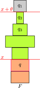
(c)

Figure 6: Visualization of Proposition B.8

This figure visualizes Proposition B.8, where LABEL:subfig:UW_Relevant1, LABEL:subfig:UW_Relevant2 and LABEL:subfig:UW_Relevant3 show the state of the algorithm at times $t^{-},t_{0}$ and $t$, correspondingly (since no changes occur in bin $P$, it is omitted from the figure). Observe that the volume covered by $x$ decreased by $p_{q_{3}}$ but increased by $p_{q}$ from $t_{0}$ to $t$. The claim in the proof of Proposition B.8 is that the volume gained by raising the bar by $\theta$ (the green volume in the figure) is at least $p_{q_{3}}$.

Proposition B.8.

Consider a call to UponJobRelease(q) at time $t$. For every $x\in\mathbb{R}^{+}\cup\left\{0\right\}$, it holds that

$$B\left(x+\theta,t\right)\geq B\left(x,t^{-}\right)+p_{q}$$

Proof.

As in the proofs of Propositions B.6 and B.7 Propositions B.6 and B.8, we denote by $t_{0}$ the time immediately after $q$’s insertion into $F$, and before the possible rotation. Consider that for every $q^{\prime}\in Q(t)\backslash\{q\}$ it holds that $\beta(q^{\prime},t_{0})=\beta(q^{\prime},t^{-})$, and thus $\gamma_{q^{\prime}}(x,t_{0})=\gamma_{q^{\prime}}(x,t^{-})$, which implies that $B\left(x,t_{0}\right)\geq B\left(x,t^{-}\right)$.

If, in addition to the previous observation, it holds that $x\geq\pi_{F}^{t_{0}}(q)$, then we have that $\gamma_{q}(x,t_{0})=p_{q}$, and thus $B\left(x,t_{0}\right)\geq B\left(x,t^{-}\right)+p_{q}$. We thus have that

$$B\left(x+\theta,t\right)\geq B\left(x,t\right)\geq B\left(x,t_{0}\right)\geq B\left(x,t^{-}\right)+p_{q}$$

where the second inequality uses Claim 2 of the proof of Proposition B.6. This completes the proof for the case that $x\geq\pi_{F}^{t_{0}}(q)$, and we thus assume for the remainder of the proof that $x<\pi_{F}^{t_{0}}(q)$.

Denote $q_{0}=q$, and let $q_{1},\cdots,q_{m}$ be the jobs involved in violations with $q$ at $t_{0}$ (it is possible that $m=0$ if there are no violations). The algorithm performs applies the cyclic permutation $\left(\pi_{F}^{t_{0}}(q_{m}),\cdots,\pi_{F}^{t_{0}}(q_{1}),\pi_{F}^{t_{0}}(q_{0})\right)$ to $\pi_{F}^{t_{0}}$ to obtain $\pi_{F}^{t}$.

As in the proof of Proposition B.6, let $i$ be the minimal index such that $\pi_{F}^{t_{0}}(q_{i})\leq x$ (due to the assumption that $\pi_{F}^{t_{0}}(q)>x$, we have that $i>0$). Due to the rotation, the volume covered by $x$ has decreased by $p_{q_{i}}$ but increased by $p_{q_{0}}$. That is, we have that

$$B\left(x,t\right)\geq B\left(x,t_{0}\right)-p_{q_{i}}+p_{q_{0}}$$

Now, it remains to show that

$$B\left(x+\theta,t\right)\geq B\left(x,t\right)+p_{q_{i}}$$ (2)

which completes the proof.

We henceforth write $q^{\star}$ instead of $q_{i}$. It holds that $x<\beta(q^{\star},t)$, and thus $\gamma_{q^{\star}}(x,t)=0$. If, in addition, we have that $\beta(q^{\star},t)\leq x+\theta$, then $\gamma_{q^{\star}}(x+\theta,t)=p_{q^{\star}}$, which implies Equation 2 and completes the proof.

Otherwise, we have that $x+\theta<\beta(q^{\star},t)$. This implies that there exist $\theta$ jobs $q^{\prime}_{1},\cdots,q^{\prime}_{\theta}\in Q_{F}(t)$, such that $\beta(q^{\prime}_{j},t)=\lfloor x+j\rfloor$ for every index $1\leq j\leq\theta$. Observe that for each index $j$ it holds that $\gamma_{q^{\prime}_{j}}(x,t)=0$ and $\gamma_{q^{\prime}_{j}}(x+\theta,t)=p_{q^{\prime}_{j}}$. Thus, it holds that

$$B\left(x+\theta,t\right)\geq B\left(x,t\right)+\sum_{j=1}^{\theta}p_{q^{\prime}_{j}}$$ (3)

It holds that $\pi_{F}^{t}(q^{\prime}_{j})\leq\pi_{F}^{t}(q^{\star})$ for each index $j$. Using Proposition B.7, we have

$$p_{q^{\prime}_{j}}\geq\tilde{p}_{q^{\prime}_{j}}\geq\frac{\tilde{p}_{q^{\star}}}{\mu}>\frac{p_{q^{\star}}}{\mu^{2}}\geq\frac{p_{q^{\star}}}{\theta}$$

Plugging into Equation 3 yields Equation 2, completing the proof. ∎

Proposition B.9.

For any $x$ and time $t$, if $B\left(x,t\right)$ is decreasing due to the algorithm’s processing of a job, then $B\left(x,t\right)=V(t)$.

Proof.

Suppose that $B\left(x,t\right)$ decreased due to the processing of a job $q\in Q_{P}(t)$ by the algorithm. This implies that $\gamma_{q}(x,t)>0$, and thus $x\geq\beta(q,t)$. But from the choice of job in Process, it holds that $\pi_{P}^{t}(q)=\delta_{P}(t)$, and thus $\beta(q,t)=\delta_{P}(t)$. Therefore, for every $q^{\prime}\in Q_{P}(t)$ it holds that $\gamma_{q^{\prime}}(x,t)=y_{q^{\prime}}(t)$.

Moreover, since the algorithm maintains that $\delta_{F}(t)\leq\delta_{P}(t)$, for every $q^{\prime}\in Q_{F}(t)$ we also have that $\gamma_{q^{\prime}}(x,t)=y_{q^{\prime}}(t)$.

Overall, we have that $B\left(x,t\right)=V(t)$, as required. ∎

This figure visualizes the inductive claim in the proof of Lemma B.10, for some time $\tau\in[0,t]$. It shows the state of the algorithm at $\tau$, placed next to the state of $Q^{*}(t,\tau)$ in the optimal solution at $\tau$. The claim is that the total volume covered by $\theta w(Q^{*}(t,\tau))$ (the orange volume) is at least the volume of $Q^{*}(t,\tau)$ in $\operatorname{OPT}$ at $\tau$ (the cyan volume).

Figure 7: Lemma B.10

Lemma B.10.

At any time $t$ it holds that $B\left(\theta\delta^{*}(t),t\right)=V(t)$.

Proof.

For any time $\tau$, let $Q^{*}(\tau)$ be the set of jobs pending in the optimal solution at time $\tau$.

We now fix a time $t$. Let $\tau$ be any time in the range $[0,t]$. We also define $Q^{*}(t,\tau)=Q^{*}(t)\cap Q^{*}(\tau)$ – i.e. the jobs alive at $t$ which were already released by $\tau$. For ease of notation we write $Y^{*}(\tau)=\sum_{q\in Q^{*}(t,\tau)}y^{*}_{q}(\tau)$.

We prove, by induction on $\tau$, that for every $\tau\in[0,t]$ it holds that

$$B\left(\theta\cdot\left|Q^{*}(t,\tau)\right|,\tau\right)\geq Y^{*}(\tau)$$ (4)

A visualization of the claim in Equation 4 appears in Figure 7.

Clearly, Equation 4 holds for $\tau=0$, as $Y^{*}(\tau)=0$. Now, we show that no possible event can break the inequality of Equation 4 as time $\tau$ progresses. When considering an event at $\tau$, we denote by $\tau^{-}$ the time immediately before the event. Consider the possible events:

1. A job moves from $F$ to $P$ in the algorithm. Proposition B.5 implies that the left-hand side of Equation 4 does not decrease upon this event. Since the right-hand side does not change, the inequality continues to hold.

2. A job $q\notin Q^{*}(t)$ is released. In this case, the right-hand side of Equation 4 remains the same. Proposition B.6 implies that the left-hand side does not decrease.

3. A job $q\in Q^{*}(t)$ is released. In this case, the right-hand side of Equation 4 increases by $p_{q}$, as $Q^{*}(t,\tau^{-})=Q^{*}(t,\tau)\cup\{q\}$. Proposition B.8 implies that

   $$B\left(\theta\cdot\left|Q^{*}(t,\tau)\right|,\tau\right)=B\left(\theta\cdot\left|Q^{*}(t,\tau^{-})\right|+\theta,\tau\right)\geq B\left(\theta\cdot\left|Q^{*}(t,\tau^{-})\right|,\tau^{-}\right)+p_{q}$$

   and thus the inequality of Equation 4 continues to hold.

4. A job $q\in Q(\tau)$ is processed. Proposition B.9 implies that if the left-hand side decreases as a result of processing, then $B\left(\theta\cdot\left|Q^{*}(t,\tau)\right|,\tau\right)=V(\tau)$. Since the algorithm is not lazy (i.e. always processes a pending job if there exists one), it holds that $V(\tau)=V^{*}(\tau)\geq Y^{*}(\tau)$, and thus the inequality holds.

The proof of the induction claim is complete. Now observe that choosing $\tau=t$, we have that $\left|Q^{*}(t,\tau)\right|=\delta^{*}(t)$ and that $Y^{*}(t)=V^{*}(t)=V(t)$. Thus, Equation 4 yields that

$$B\left(\theta\delta^{*}(t),t\right)=V(t)$$

completing the proof. ∎

Proof of Theorem 4.2.

Lemma B.10 implies that at any time $t$ we have $B\left(\theta\delta^{*}(t),t\right)=V(t)$. This implies that $\delta_{F}(t)\leq\theta\delta^{*}(t)$; otherwise, there would exist a pending job $q\in Q_{F}(t)$ such that $\beta(q,t)>\theta\delta^{*}(t)$, the volume of which would not be counted in $B\left(\theta\delta^{*}(t),t\right)$. The same argument applies to $P$ as well, yielding that $\delta_{P}(t)\leq\theta\delta^{*}(t)$.

Overall, we get that $\delta(t)\leq 2\theta\delta^{*}(t)$. Integrating over $t$ completes the proof of the theorem.

∎

B.2 Proof of Theorem 4.3

In the following analysis, we prove Theorem 4.3.

Definition B.11 (time-dependent variable values).

For any time $t$, we define $Q_{F^{i}}(t)$ and $Q_{P^{i}}(t)$ to be the values of the variables $Q_{F^{i}}$ and $Q_{P^{i}}$ at time $t$, respectively. We define $Q_{A^{i}}(t)=Q_{F^{i}}(t)\cup Q_{P^{i}}(t)$, which is the set of pending jobs in superbin $A^{i}$ at time $t$.

We also define $\pi_{F^{i}}^{t}$ and $\pi_{P^{i}}^{t}$ to be the values of the priority-mapping variables $\pi_{F^{i}}$ and $\pi_{P^{i}}$ at time $t$.

Definition B.12 (base of a job).

For every time $t$ and every job $q\in Q_{F^{i}}(t)$, we define the base of $q$ at time $t$ as follows:

$$X(q,t)=\left\{q^{\prime}\in Q_{F^{i}}(t)\middle|\pi_{F^{i}}^{t}(q^{\prime})\leq\pi_{F^{i}}^{t}(q)\right\}$$

For ease of notation, we denote $w(X(q,t))$ by $\beta(q,t)$. For every job $q\in Q_{P^{i}}(t)$, we similarly define $X(q,t)$ and $\beta(q,t)$ according to $\pi_{P^{i}}^{t}$.

We now redefine the volume covered by a bar $x$.

Definition B.13 (Volume covered by bar).

For any $x\in\mathbb{R}^{+}\cup\left\{0\right\}$ and time $t$, and for any job $q\in Q(t)$, we define

$$\gamma_{q}(x,t)=\begin{cases}y_{q}(t)&x\geq\beta(q,t)\\ 0&\text{otherwise}\par\end{cases}$$

called the volume of $q$ covered by $x$ at $t$.

For every superbin index $i$, we define the total volume covered by $x$ in various bins:

• $B_{F^{i}}\left(x,t\right)=\sum_{q\in Q_{F^{i}}(t)}\gamma_{q}(x,t)$

• $B_{P^{i}}\left(x,t\right)=\sum_{q\in Q_{P^{i}}(t)}\gamma_{q}(x,t)$

• $B_{A^{i}}\left(x,t\right)=B_{F^{i}}\left(x,t\right)+B_{P^{i}}\left(x,t\right)$

• $B\left(x,t\right)=\sum_{i}B_{A^{i}}\left(x,t\right)$

Figure 8 visualizes Definition B.13, where $B\left(x,t\right)$ is the total orange area in the figure.

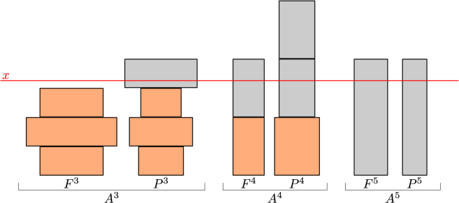
Figure 8: Visualization of Covered Volume

For ease of notation, we again define $\theta=\left\lceil(1+\epsilon)^{2}\right\rceil$.

Proposition B.14.

Upon the release of a job $q$ at time $t$, and for every $x\in\mathbb{R}^{+}\cup\left\{0\right\}$, it holds that

• $B\left(x,t\right)\geq B\left(x,t^{-}\right)$

• $B\left(x+\theta w_{q},t\right)\geq B\left(x,t^{-}\right)+p_{q}$

Proof.

Let $i$ be such that $w_{q}=2^{i}$. The job $q$ is thus sent to the superbin $A^{i}$.

To prove the first claim, first note that the structure of every superbin $A^{i^{\prime}}$ for $i^{\prime}\neq i$ remains the same after $q$’s release. Thus, we have that $B_{A^{i^{\prime}}}\left(x,t\right)=B_{A^{i^{\prime}}}\left(x,t^{-}\right)$. As for the volume covered in $A^{i}$, we know that it does not decrease due to Proposition B.6 (it is easy to verify that this proposition holds when all weights are scaled up by $2^{i}$).

To prove the second item, again note that for every $i^{\prime}\neq i$ it holds that $B_{A^{i^{\prime}}}\left(x+\theta w_{q},t\right)\geq B_{A^{i^{\prime}}}\left(x,t\right)=B_{A^{i^{\prime}}}\left(x,t^{-}\right)$. As for the volume covered in $A^{i}$, using Proposition B.8 (scaled up by $2^{i}$) yields that $B_{A^{i}}\left(x+\theta w_{q},t\right)\geq B_{A^{i}}\left(x,t^{-}\right)+p_{q}$. This completes the proof. ∎

Proposition B.15.

For any $x$ and time $t$, if $B\left(x,t\right)$ is decreasing due to the algorithm’s processing of a job, then $B\left(x,t\right)=V(t)$.

Proof.

Consider the job $q$ being processed, where $q\in P^{i}$ for some $i$. Since $\gamma_{q}(x,t)>0$, we have that $x\geq\beta(q,t)$. Since the algorithm processes the job $q\in Q_{P^{i}}(t)$ such that $\pi_{P^{i}}^{t}(q)=\delta_{P^{i}}(t)$, we have that $\beta(q,t)=\delta_{P^{i}}(t)\cdot 2^{i}=w(Q_{P^{i}}(t))$.

Now, observe that since the algorithm chose superbin $A^{i}$ for processing, it must be that for every $i^{\prime}$ we have $w(Q^{i}_{P}(t))\geq w(Q^{i^{\prime}}_{P}(t))\geq w(Q^{i^{\prime}}_{F}(t))$, where the second inequality is since the algorithm moves jobs from the full bins to the partial bins.

Since $x$ is at least the weight of every bin in the system, it is at least $\beta(q^{\prime},t)$ for every $q^{\prime}\in Q(t)$, and thus $B\left(x,t\right)=V(t)$. ∎

Lemma B.16.

At any time $t$ it holds that $B\left(\theta\cdot w(Q^{*}(t)),t\right)=V(t)$.

Proof.

The proof of this lemma is nearly identical to that of Lemma B.10 of Subsection 4.1, but uses the propositions of this subsection instead.

We now fix a time $t$. Let $\tau$ be any time in the range $[0,t]$. We again define $Q^{*}(t,\tau)$ and $Y^{*}(\tau)$ as in the proof of Lemma B.10.

We prove, by induction on $\tau$, an identical claim to that in the proof of Lemma B.10, which is that for every $\tau\in[0,t]$ it holds that

$$B\left(\theta\cdot\left|Q^{*}(t,\tau)\right|,\tau\right)\geq Y^{*}(\tau)$$ (5)

The claim trivially holds for time $\tau=0$, before any requests were released. We now consider the possible events which could possibly break the claim as $\tau$ progresses, in a similar way to Lemma B.10.

1. A job moves from $F$ to $P$ in the algorithm. Proposition B.5 implies that the left-hand side of Equation 5 does not decrease upon this event. Since the right-hand side does not change, the inequality continues to hold.

2. A job $q\notin Q^{*}(t)$ is released. In this case, the right-hand side of Equation 5 remains the same. The first claim in Proposition B.14 implies that the left-hand side does not decrease.

3. A job $q\in Q^{*}(t)$ is released. In this case, the right-hand side of Equation 5 increases by $p_{q}$, as $Q^{*}(t,\tau^{-})=Q^{*}(t,\tau)\cup\{q\}$. The second claim in Proposition B.14 implies that

   $$B\left(\theta\cdot w(Q^{*}(t,\tau)),\tau\right)=B\left(\theta\cdot w(Q^{*}(t,\tau^{-}))+\theta w_{q},\tau\right)\geq B\left(\theta\cdot w(Q^{*}(t,\tau^{-})),\tau^{-}\right)+p_{q}$$

   and thus the inequality of Equation 5 continues to hold.

4. A job $q\in Q(\tau)$ is processed. Proposition B.15 implies that if the left-hand side decreases as a result of processing, then $B\left(\theta\cdot\left|Q^{*}(t,\tau)\right|,\tau\right)=V(\tau)$. Since the algorithm is not lazy (i.e. always processes a pending job if there exists one), it holds that $V(\tau)=V^{*}(\tau)\geq Y^{*}(\tau)$, and thus the inequality holds.

The proof of the induction claim is now complete, and choosing $\tau=t$ in Equation 5 yields

$$B\left(\theta\delta^{*}(t),t\right)=V(t)$$

as required. ∎

Proof of Theorem 4.3.

At any time $t$, the algorithms contains at most $\left\lceil\log W\right\rceil+1$ nonempty superbins, each of which contains two bins (full and partial). From Lemma B.16, at any time $t$, there does not exist a pending job $q$ in the algorithm such that $\beta(q,t)>\theta\cdot w(Q^{*}(t))$. Thus, the total weight in each bin is at most $\theta\cdot w(Q^{*}(t))$, and thus $2\theta\cdot w(Q^{*}(t))$ for each superbin (which contains two bins). Overall, the total weight in the system is at most $2\theta(\left\lceil\log W\right\rceil+1)w(Q^{*}(t))$.

Integrating over $t$ thus yields the desired result, which is that the algorithm is $O(\theta\log W)$ competitive. ∎

Appendix C Lower Bound for Unweighted sppt

In this section, we show a lower bound of $2$ on the competitive ratio of any algorithm for sppt, even when the distortion parameter is arbitrarily close to $1$. This lower bound is perhaps somewhat surprising, as one would hope that as $\mu$ approaches $1$, one would be able to approximate the optimal SRPT schedule, and thus approach $1$-competitiveness.

Theorem C.1.

For any $\mu>1$, there is no deterministic $\mu$-robust algorithm with competitive ratio less than $2$.

Proof.

Fix some $\mu>1$. We assume that $\mu\leq 2$, as we are interested in the case of $\mu$ approaching $1$ (clearly if the lower bound holds for small $\mu$, it holds for large $\mu$).

Let $\lambda=\frac{\mu+1}{\mu-1}$, and let $M$ be an arbitrarily large integer. The adversary we describe operates in $M$ phases, numbered from $M-1$ down to $0$. Phase $i$ takes $\lambda^{i}$ time units. Observe the following adversary:

1. for $i$ from $M-1$ to $0$:

   1. release two jobs of predicted processing time $\lambda^{i}$.

   2. wait $\lambda^{i}$ time units.

   3. of the two jobs released in this phase, let $q_{1}^{i}$ be the job processed more by the algorithm during these $\lambda^{i}$ time units, and let $q_{2}^{i}$ be the other job. The adversary sets $p_{q_{1}^{i}}=\mu\lambda^{i}$ and $p_{q_{2}^{i}}=\lambda^{i}$.

During phase $i$, the algorithm has processed job $q_{1}^{i}$ for at most $\frac{\lambda^{i}}{2}$ time, and has processed job $q_{2}^{i}$ for at most $\lambda^{i}$ time. Thus, both $q_{1}^{i}$ and $q_{2}^{i}$ have remaining volume of $(\mu-1)\lambda^{i}=(\mu+1)\lambda^{i-1}$ at the end of the phase. Also observe that the total time of phases $i-1$ through $0$ is at most

$$\sum_{i^{\prime}=0}^{\infty}\lambda^{i-1-i^{\prime}}=\lambda^{i-1}\cdot\frac{1}{1-\lambda^{-1}}=\lambda^{i-1}\cdot\frac{1-\mu}{2}$$

And thus, at the end of the last phase, it must be that the remaining processing time for both $q_{1}^{i}$ and $q_{2}^{i}$ in the algorithm is at least $\frac{1-\mu}{2}\lambda^{i-1}$.

Overall, we have that the algorithm has $2M$ living jobs at the end of the $M$ phases, each with at least $\frac{1-\mu}{2}\lambda^{0}=\frac{1-\mu}{2}$ remaining volume. The optimal solution, on the other hand, has $M$ living jobs, as it would complete $q_{2}^{i}$ in each phase $i$.

Now, after the $M$ phases, the adversary would begin the “bombardment”, releasing a job of processing time $x=\frac{1-\mu}{2}$ every $x$ time units. The algorithm would have no option which is better than serving the “bombardment” requests, and the optimal solution would do the same. During the bombardment, the algorithm has $2M+1$ living jobs at any time, and the optimal solution has $M+1$. Thus, the competitive ratio tends to $\frac{2M+1}{M+1}$ as the bombardment continues. Since $M$ was chosen arbitrarily, we can let $M$ tend to $\infty$, and thus the competitive ratio tends to $2$. ∎

Appendix D Semiclairvoyant Scheduling

In the semiclairvoyant model, we are given the logarithmic class of a job rather than an estimate for its processing time. That is, for a job $q$ the algorithm is given $\ell_{q}=\left\lfloor\log_{\rho}p_{q}\right\rfloor$ and not $p_{q}$ (for a constant $\rho>1$).

Clearly, this model can be reduced to the prediction model as follows. Upon the arrival of $q$, define $\tilde{p}_{q}=\rho^{\ell_{q}}$ and $\mu=\rho$. From the definition of class, it is clear that indeed $p_{q}\in\left[\tilde{p}_{q},\mu\tilde{p}_{q}\right)$.

Denote the semiclairvoyant model with the parameter $\rho$ by ${\mathrm{SC}}_{\rho}$. Applying the theorems of this paper for sppt, we immediately obtain the first results for weighted flow time in the semiclairvoyant setting.

Corollary D.1 (of Theorems 4.3, 3.1 and 3.11).

In the ${\mathrm{SC}}_{\rho}$ model, there exist:

1. An $O(\log P)$-competitive algorithm (using Theorem 3.1)

2. An $O(\log D)$-competitive algorithm (using Theorem 3.11)

3. An $O(\log W)$-competitive algorithm (using Theorem 4.3)

Note that these results for the semiclairvoyant setting match the best known results for the clairvoyant setting, in terms of all three parameters $P,D,W$.

In addition, we consider the algorithm in Subsection 4.1 for unweighted sppt, and show that for the ${\mathrm{SC}}_{\rho}$ model it obtains an improved competitive ratio, which is $2\left\lceil\rho\right\rceil$. In particular, when $\rho=2$ this algorithm is $4$ competitive, improving upon the $13$-competitive algorithm of [6].

D.1 Unweighted Semiclairvoyant Scheduling

We now show the following theorem for the competitiveness of the algorithm of Subsection 4.1 for the unweighted semiclairvoyant setting.

Theorem D.2.

In the ${\mathrm{SC}}_{\rho}$ model, the competitive ratio of the algorithm of Subsection 4.1 is $2\left\lceil\rho\right\rceil$.

Corollary D.3.

In the ${\mathrm{SC}}_{2}$ model (i.e. base-2 classes) the algorithm of Subsection 4.1 is $4$-competitive.

As observed before, we have that $\mu=\rho$.

For ease of notation, we define $\theta^{\prime}=\left\lceil\mu\right\rceil=\left\lceil\rho\right\rceil$. The proof of Theorem D.2 is identical to that of Theorem 4.2, except for replacing Proposition B.8 with the following proposition.

Proposition D.4 (stronger version of Proposition B.8).

Consider a call to UponJobRelease(q) at time $t$. For every $x\in\mathbb{R}^{+}\cup\left\{0\right\}$, it holds that

$$B\left(x+\theta^{\prime},t\right)\geq B\left(x,t^{-}\right)+p_{q}$$

Proof.

The proof is identical to the proof of Proposition B.8, except for replacing the claim that

$$B\left(x+\theta,t\right)\geq B\left(x,t\right)+p_{q^{\prime}}$$

with the stronger claim that

$$B\left(x+\theta^{\prime},t\right)\geq B\left(x,t\right)+p_{q^{\prime}}$$

with $q^{\prime}$ defined as in the proof of Proposition B.8.

From the definition of $q^{\prime}$ in the original proof, it holds that $\beta(q^{\prime},t)>x$, and thus $\gamma_{q^{\prime}}(x,t)=0$. If $\beta(q^{\prime},t)\leq x+\theta^{\prime}$, then $\gamma_{q^{\prime}}(x+\theta^{\prime},t)=p_{q^{\prime}}$, and the proof is complete.

Otherwise, it holds that $\beta(q^{\prime},t)>x+\theta^{\prime}$. Consider the $\theta^{\prime}$ distinct jobs $q_{1},\cdots,q_{\theta^{\prime}}\in Q_{F}(t)$ such that $\beta(q_{j},t)=x+j$ for each index $j$. Observe that for each index $j$ it holds that $\gamma_{q_{j}}(x,t)=0$ and $\gamma_{q_{j}}(x+\theta^{\prime},t)=p_{q_{j}}$. Thus, it holds that

$$B\left(x+\theta^{\prime},t\right)\geq B\left(x,t\right)+\sum_{j=1}^{\theta^{\prime}}p_{q_{j}}$$ (6)

It holds that $\pi_{F}^{t}(q^{\prime})>\pi_{F}^{t}(q_{j})$ for each $j$. Using Proposition B.7, we have that the state of the algorithm at time $t$ contains no violations. However, observe that if $\ell_{q_{j}}<\ell_{q^{\prime}}$, then we have that

$$\rho\tilde{p}_{q_{j}}=\rho\cdot\rho^{\ell_{q_{j}}}=\rho^{\ell_{q_{j}}+1}\leq\rho^{\ell_{q^{\prime}}}=\tilde{p}_{q^{\prime}}$$

which is a violation, in contradiction to Proposition B.7. Thus, for every $j$ it holds that $\ell_{q_{j}}\geq\ell_{q}$, and thus $p_{q_{j}}\geq\tilde{p}_{q_{j}}\geq\rho^{\ell_{q_{j}}}\geq\rho^{\ell_{q^{\prime}}}\geq\frac{p_{q^{\prime}}}{\rho}\geq\frac{p_{q^{\prime}}}{\theta^{\prime}}$.

Plugging into Equation 6, we get

$$B\left(x+\theta^{\prime},t\right)\geq B\left(x,t\right)+p_{q^{\prime}}$$

completing the proof. ∎

This completes the proof of Theorem D.2.

Appendix E Proof of Theorem 3.11

This section proves Theorem 3.11.

Observe that the maximum ratio of estimated densities (i.e. $\frac{w_{q}}{\tilde{p}_{q}}$) with respect to the original weight (before rounding) is at most $\mu D$. After rounding up to powers of $\lambda$, which is $\Theta(\mu)$, we have that the maximum ratio of densities becomes $O(\mu^{2}D)$. Hence, the maximum ratio of estimated ei-density values is also $O(\mu^{2}D)$. We thus define the number of ei-density classes to be $\Lambda^{\prime}$, and observe that $\Lambda^{\prime}=O(\log(\mu^{2}D)=O(\log(\mu D))$.

The following lemma immediately implies Theorem 3.11, in the same manner in which Lemma 3.4 implied Theorem 3.1.

Lemma E.1 (analogue of Lemma 3.4).

At any point in time $t$, it holds that $W\left(t\right)\leq O(\Lambda^{\prime}\mu^{2})\cdot W^{*}\left(t\right)$.

Proof of Lemma E.1.

As noted in the proof of Lemma 3.4, we have $\operatorname{clw}\left(t\right)\leq i^{*}$. Define $j_{\min}$ and $j_{\max}$ to be the minimum and maximum ei-density classes, respectively. We have

$$W\left(t\right) =\sum_{j=j_{\min}}^{j_{\max}}W_{\leq i^{*},=j}\left(t\right)$$

$$\leq 2(j_{\max}-j_{\min}+1)u_{i^{*}}+2\mu W^{*}\left(t\right)+\sum_{j=j_{\min}}^{j_{\max}}2\max\left\{0,\frac{\Delta V_{\leq i^{*},\leq j}\left(t\right)missing}{2^{j}}\right\}$$

$$\leq 2\Lambda^{\prime}u_{i^{*}}+2\mu W^{*}\left(t\right)+\sum_{j=j_{\min}}^{j_{\max}}8\mu\cdot u_{\operatorname{clw}\left(t_{j}\right)}$$

using the same arguments as in the proof of Lemma 3.4. Now, observe that for every ei-density class $j$ we have $\operatorname{clw}\left(t_{j}\right)\leq i^{*}$ from Proposition 3.10. Thus

$$W\left(t\right) \leq(8\mu+2)\Lambda^{\prime}u_{i^{*}}+2\mu W^{*}\left(t\right)\leq O(\Lambda^{\prime}\mu^{2})W^{*}\left(t\right)\qed$$

References

- [1] Yossi Azar and Noam Touitou. Improved online algorithm for weighted flow time. In Mikkel Thorup, editor, 59th IEEE Annual Symposium on Foundations of Computer Science, FOCS 2018, Paris, France, October 7-9, 2018, pages 427–437. IEEE Computer Society, 2018.
- [2] Nikhil Bansal and Ho-Leung Chan. Weighted flow time does not admit o(1)-competitive algorithms. In Proceedings of the Twentieth Annual ACM-SIAM Symposium on Discrete Algorithms, SODA 2009, New York, NY, USA, January 4-6, 2009, pages 1238–1244, 2009.
- [3] Nikhil Bansal and Kedar Dhamdhere. Minimizing weighted flow time. ACM Trans. Algorithms, 3(4):39, 2007. also in SODA 2003: 508-516.
- [4] Nikhil Bansal, Kedar Dhamdhere, Jochen Könemann, and Amitabh Sinha. Non-clairvoyant scheduling for minimizing mean slowdown. Algorithmica, 40(4):305–318, 2004.
- [5] Luca Becchetti and Stefano Leonardi. Non-clairvoyant scheduling to minimize the average flow time on single and parallel machines. In Proceedings of the thirty-third annual ACM symposium on Theory of computing, pages 94–103, 2001.
- [6] Luca Becchetti, Stefano Leonardi, Alberto Marchetti-Spaccamela, and Kirk Pruhs. Semi-clairvoyant scheduling. Theor. Comput. Sci., 324(2-3):325–335, 2004.
- [7] Michael A. Bender, S. Muthukrishnan, and Rajmohan Rajaraman. Improved algorithms for stretch scheduling. In David Eppstein, editor, Proceedings of the Thirteenth Annual ACM-SIAM Symposium on Discrete Algorithms, January 6-8, 2002, San Francisco, CA, USA, pages 762–771. ACM/SIAM, 2002.
- [8] Chandra Chekuri, Sanjeev Khanna, and An Zhu. Algorithms for minimizing weighted flow time. In Proceedings on 33rd Annual ACM Symposium on Theory of Computing, July 6-8, 2001, Heraklion, Crete, Greece, pages 84–93, 2001.
- [9] Sungjin Im, Janardhan Kulkarni, and Kamesh Munagala. Competitive algorithms from competitive equilibria: Non-clairvoyant scheduling under polyhedral constraints. Journal of the ACM (JACM), 65(1):1–33, 2017.
- [10] Sungjin Im, Janardhan Kulkarni, Kamesh Munagala, and Kirk Pruhs. Selfishmigrate: A scalable algorithm for non-clairvoyantly scheduling heterogeneous processors. In 2014 IEEE 55th Annual Symposium on Foundations of Computer Science, pages 531–540. IEEE, 2014.
- [11] Jae-Hoon Kim and Kyung-Yong Chwa. Non-clairvoyant scheduling for weighted flow time. Inf. Process. Lett., 87(1):31–37, 2003.
- [12] Silvio Lattanzi, Thomas Lavastida, Benjamin Moseley, and Sergei Vassilvitskii. Online scheduling via learned weights. In Proceedings of the Thirty-First Annual ACM-SIAM Symposium on Discrete Algorithms, SODA 2020, New Orleans, LA, USA, January 5 - 8, 2020., 2020.
- [13] Thodoris Lykouris and Sergei Vassilvitskii. Competitive caching with machine learned advice. In Proceedings of the 35th International Conference on Machine Learning, ICML 2018, Stockholmsmässan, Stockholm, Sweden, July 10-15, 2018, pages 3302–3311, 2018.
- [14] Andres Muñoz Medina and Sergei Vassilvitskii. Revenue optimization with approximate bid predictions. In Advances in Neural Information Processing Systems 30: Annual Conference on Neural Information Processing Systems 2017, 4-9 December 2017, Long Beach, CA, USA, pages 1858–1866, 2017.
- [15] Michael Mitzenmacher. Queues with small advice. CoRR, abs/2006.15463, 2020.
- [16] Michael Mitzenmacher. Scheduling with Predictions and the Price of Misprediction. In Thomas Vidick, editor, 11th Innovations in Theoretical Computer Science Conference (ITCS 2020), volume 151 of Leibniz International Proceedings in Informatics (LIPIcs), pages 14:1–14:18, Dagstuhl, Germany, 2020. Schloss Dagstuhl–Leibniz-Zentrum fuer Informatik.
- [17] Michael Mitzenmacher and Sergei Vassilvitskii. Algorithms with predictions. arXiv preprint arXiv:2006.09123, 2020.
- [18] Rajeev Motwani, Steven Phillips, and Eric Torng. Nonclairvoyant scheduling. Theoretical computer science, 130(1):17–47, 1994.
- [19] Manish Purohit, Zoya Svitkina, and Ravi Kumar. Improving online algorithms via ml predictions. In Advances in Neural Information Processing Systems, pages 9661–9670, 2018.
- [20] Wayne E. Smith. Various optimizers for single-stage production. Naval Research Logistics Quarterly, 3(1-2):59–66, 1956.
- [21] Jianqiao Zhu, Ho-Leung Chan, and Tak Wah Lam. Non-clairvoyant weighted flow time scheduling on different multi-processor models. Theory Comput. Syst., 56(1):82–95, 2015.