Precision Nucleon Charges and Form Factors Using 2+1-flavor Lattice QCD

Abstract

We present a high statistics study of the isovector nucleon charges and form factors using seven ensembles of 2+1-flavor Wilson-clover fermions. The axial vector and pseudoscalar form factors obtained on each of these ensembles satisfy the partially conserved axial current relation between them once the lowest energy $N\pi$ excited state is included in the spectral decomposition of the correlation functions used for extracting the ground state matrix elements. Similarly, we find evidence that the $N\pi\pi$ excited state contributes to the correlation functions with the insertion of the vector current, consistent with the vector meson dominance model. The resulting form factors are consistent with the Kelly parameterization of the experimental electric and magnetic data. Our final estimates for the isovector charges are $g_{A}^{u-d}=1.32(6)(5)_{\rm sys}$, $g_{S}^{u-d}=1.06(9)(6)_{\rm sys}$, and $g_{T}^{u-d}=0.97(3)(2)_{\rm sys}$, where the first error is the overall analysis uncertainty and the second is an additional combined systematic uncertainty. The form factors yield: (i) the axial charge radius squared, ${\langle r_{A}^{2}\rangle}^{u-d}=0.428(53)(30)_{\rm sys}\ {\rm fm}^{2}$, (ii) the induced pseudoscalar charge, $g_{P}^{\ast}=7.9(7)(9)_{\rm sys}$, (iii) the pion-nucleon coupling $g_{\pi{\rm NN}}=12.4(1.2)$, (iv) the electric charge radius squared, ${\langle r_{E}^{2}\rangle}^{u-d}=0.85(12)(19)_{\rm sys}\ {\rm fm}^{2}$, (v) the magnetic charge radius squared, ${\langle r_{M}^{2}\rangle}^{u-d}=0.71(19)(23)_{\rm sys}\ {\rm fm}^{2}$, and (vi) the magnetic moment $\mu^{u-d}=4.15(22)(10)_{\rm sys}$. All our results are consistent with phenomenological/experimental values but with larger errors. Last, we present a Padé parameterization of the axial, electric and magnetic form factors over the range $0.04<Q^{2}<1$ GeV² for phenomenological studies.

I Introduction

The success of high precision experiments such as DUNE at Fermilab Abi et al. (2018); Acciarri et al. (2015) and the T2T-HyperK in Japan Abe et al. (2018); hyp (2020) is predicated on precise determination of the flux of the neutrino beam, incident neutrino energy and their cross sections off nuclear targets. A major source of uncertainty in the analysis of neutrino-nucleus interactions is the axial vector form factors of the nucleon and appropriate nuclear corrections. Steady improvements in lattice quantum chromodynamics (QCD) calculations are expected to provide first principle results with control over all systematics Kronfeld et al. (2019). In this paper, we present high statistics results for the matrix elements of the isovector axial and vector current between ground state nucleons. From these we extract the axial, electric, and magnetic form factors and charges that are inputs in the analysis of the charged current lepton-nucleus scattering utilizing electron, muon and neutrino beams. A heuristic parameterization of the form factors for phenomelogical analyses is summarized in Eqs. (55), (56) and (58).

In previous publications, we have presented results for the isovector charges, $g_{A}^{u-d}$, $g_{S}^{u-d}$ and $g_{T}^{u-d}$ Gupta et al. (2018); axial, $G_{A}(Q^{2})$, induced pseudoscalar, $\widetilde{G}_{P}(Q^{2})$ and pseudoscalar, $G_{P}(Q^{2})$, form factors Gupta et al. (2017); Jang et al. (2020a); and the electric and magnetic form factors, $G_{E}(Q^{2})$ and $G_{M}(Q^{2})$ Jang et al. (2020b). Those calculations were done using the clover-on-HISQ formulation, i.e., the Wilson-clover fermion action was used to construct correlation functions on background gauge configurations generated with 2+1+1 flavors of the highly improved staggered quark (HISQ) action by the MILC Collaboration Bazavov et al. (2013). They exposed a number of issues that require attention: The central value for the isovector axial charge $g_{A}^{u-d}=1.218(25)(30)$ Gupta et al. (2018), a key parameter that encapsulates the strength of weak interactions of nucleons, is about 5% below the accurately measured value $\lambda=g_{A}/g_{V}=1.27641(45)_{\rm stat}(33)_{\rm sys}$ Märkisch et al. (2019); Brown et al. (2018); Mendenhall et al. (2013); Mund et al. (2013). Second, the axial and pesudoscalar form factors, $G_{A}$, $\widetilde{G}_{P}$ and $G_{P}$, did not satisfy the relation imposed on them by the partially conserved axial current (PCAC) relation Gupta et al. (2017), whereas the original three-point correlation functions did. Third, the electric and magnetic form factors, $G_{E}$ and $G_{M}$, showed significant deviations from the Kelly parameterization, which accurately describes the experimental data Jang et al. (2020b). Last, while the uncertainty in the scalar and tensor charges, $g_{S}^{u-d}=1.022(80)(60)$ and $g_{T}^{u-d}=0.989(30)(10)$, was reduced to $O(10\%)$ as required to put constraints on novel scalar and tensor interactions at the $O(10^{-3})$ level Bhattacharya et al. (2012) that can arise at the TeV scale, future experiments targeting $O(10^{-4})$ sensitivity require the reduction of errors to a few percent level.

In this paper, we revisit these issues with high-statistics calculations on seven ensembles with similar lattice parameters but generated using 2+1 flavor Wilson-Clover fermions by the JLab/W&M/LANL/MIT Collaborations Edwards et al. (2016). Three important improvements are made over those presented in our previous papers Gupta et al. (2018, 2017); Jang et al. (2020a, b). First, these calculations have been done using a unitary, clover-on-clover, lattice formulation, whereas possible systematics in the clover-on-HISQ mixed action calculations due to the nonunitarity formulation were not explored. Second, the results are based on much higher statistics, $O(2\hbox{--}6\times 10^{5})$ measurements on $O(2\hbox{--}5\times 10^{3})$ configurations. The resulting smaller errors in the raw data provide more reliable control over the systematics. Last, we compare several analysis strategies to control excited-state contamination (ESC) and quantify the sensitivity of the results to different theoretically motivated values of the mass gaps, and investigate the possible excited states that may be contributing.

Results for the nucleon charges from a subset of the ensembles analyzed here have been presented in Refs. Yoon et al. (2016, 2017). In parts of the paper, we will drop, for brevity, the superscripts $(u-d)$ to denote isovector quantities since all the analyses presented here are restricted to this case. We will, however, include this superscript in the final results and at appropriate places to avoid confusion for the general reader. For the overall methodology used to calculate the two- and three-point correlation functions, we refer the reader to our previous work Gupta et al. (2018, 2017); Jang et al. (2020b).

This paper is organized as follows. After a review of the phenomenology and known results in Sec. II and the lattice setup and error analysis strategy in Sec. III, we briefly summarize the main systematics that need to be resolved in Sec. IV. The analysis of excited states in the two-point functions is discussed in Sec. V, and in three-point functions in Sec. VI. The relations for the extraction of form factors from ground state matrix elements are given in Sec. VII and the results for the isovector charges $g_{A,S,T}^{u-d}$ in Sec. VIII. The analysis of the $A_{4}$ correlator, $\langle\Omega|{\mathcal{N}}(\tau)A_{4}(t){\mathcal{N}}(0)|\Omega\rangle$, and the consequent description of the strategies used for controlling ESC in the axial channel are discussed in Sec. IX. The extraction of the axial form factors is then presented in Sec. X followed by the parameterization of the $Q^{2}$ dependence of $G_{A}(Q^{2})$ and the extraction of $g_{A}$ and $\langle r_{A}^{2}\rangle$ in Sec. X.1, and of the induced pseudoscalar form factor ${\widetilde{G}}_{P}(Q^{2})$ and the couplings $g_{P}^{\ast}$ and $g_{\pi NN}$ in Sec. XI. Sec. XII is devoted to the electromagnetic form factors. Final estimates at the physical point defined by $a=0$, $M_{\pi}=135$ MeV and $M_{\pi}L=\infty$ are obtained using simultaneous chiral-continuum-finite-volume (CCFV) fits in Sec. XIII. An alternate heuristic parameterization of the form factors is given in Sec. XIV, and the comparison with previous work and phenomenology in Sec. XV. Our conclusions are presented in Sec. XVI. Further details of the data, analyses, and figures are presented in eight appendixes.

II Phenomenology

One of the main uncertainties in the phenomenological analyses of neutrino-nucleon scattering is the knowledge of the axial form factors. Direct experiments using liquid hydrogen (proton) targets are not being carried out due to safety concerns. Thus, phenomenologists are looking to lattice QCD to provide first principle estimates. A good validation of the lattice methodology for the calculation of form factors is to demonstrate agreement between the simultaneously calculated isovector electric and magnetic form factors with the Kelly (or other good) parameterization of the accurate experimental data (see Sec. XII). Furthermore, calculating the full set of axial and electromagnetic form factors is the first step in the analysis of the charged current neutrino-nucleon cross section with all required input taken from lattice QCD. Our results in Eqs. (55) (56) and (58) represent significant progress toward this goal.

The matrix element of the isovector axial vector current $A_{\mu}=\overline{u}\gamma_{\mu}\gamma_{5}d$ between ground state nucleons, which describes neutron $\beta$-decay and the weak charged current of the interaction of the neutrino with the nucleon, has the following relativistically covariant decomposition in terms of two form factors:

$$\left\langle N({\bm{p}}_{f},s_{f})|A_{\mu}(\bm{q})|N({\bm{p}}_{i},s_{i})\right\rangle=\\ {\overline{u}}_{N}({\bm{p}}_{f},s_{f})\left(G_{A}(q^{2})\gamma_{\mu}+q_{\mu}\frac{\widetilde{G}_{P}(q^{2})}{2M_{N}}\right)\gamma_{5}u_{N}({\bm{p}}_{i},s_{i}),$$ (1)

where $G_{A}(q^{2})$ is the axial vector form factor, $\widetilde{G}_{P}(q^{2})$ the induced pseudoscalar form factor, $|N({\bm{p}}_{f},s_{f})\rangle$ the nucleon state with momentum ${\bm{p}}_{f}$ and spin $s_{f}$, and the momentum transfer is $\bm{q}={\bm{p}}_{f}-{\bm{p}}_{i}$. Throughout this paper, all data for the form factors are presented in terms of $Q^{2}\equiv{\bf p}^{2}-(E-m)^{2}=-q^{2}$, i.e., the spacelike four-momentum squared. We use the DeGrand-Rossi basis for the gamma matrices DeGrand and Rossi (1990), and assume isospin symmetry, $m_{u}=m_{d}$. Thus, we neglect the induced tensor form factor $\widetilde{G}_{T}$ that vanishes in the isospin limit Bhattacharya et al. (2012). The axial charge $g_{A}\equiv G_{A}(q^{2}=0)$ is obtained from both the forward matrix element and by extrapolating $G_{A}(Q^{2})$ to $Q^{2}=0$ as discussed in Secs. VIII, and XIII.1, respectively.

The pseudoscalar form factor, $G_{P}$, is defined by

$$\left\langle N({\bm{p}}_{f})|P(\bm{q})|N({\bm{p}}_{i})\right\rangle={\overline{u}}_{N}({\bm{p}}_{f})G_{P}(q^{2})\gamma_{5}u_{N}({\bm{p}}_{i})\,,$$ (2)

where $P=\overline{u}\gamma_{5}d$ is the pseudoscalar density.

The discrete lattice momenta are given by $2\pi{\bf n}/La$ with the components of the vector ${\bf n}\equiv(n_{1},n_{2},n_{3})$ taking on integer values, $|n_{i}|\in\{0,L\}$. The normalization of the nucleon spinors $u_{N}(\bm{p},s)$ in Euclidean space is

$$\sum_{s}u_{N}(\bm{p},s)\bar{u}_{N}({\bm{p}},s)=\frac{E({\bm{p}})\gamma_{4}-i\bm{\gamma}\cdot{\bm{p}}+M}{2E({\bm{p}})}\,.$$ (3)

The three form factors, $G_{A}(Q^{2})$, $\widetilde{G}_{P}(Q^{2})$ and ${G}_{P}(Q^{2})$, are not independent because of the PCAC operator identity, $\partial_{\mu}A_{\mu}-2{\widehat{m}}P=0$. By contracting Eq. (1) with $q^{\mu}$ and using Eq. (2), this identity gives the following relation between them:

$$2{\widehat{m}}G_{P}(Q^{2})=2M_{N}G_{A}(Q^{2})-\frac{Q^{2}}{2M_{N}}{\widetilde{G}}_{P}(Q^{2})\,,$$ (4)

where ${\widehat{m}}\equiv Z_{m}Z_{P}(m_{u}+m_{d})/(2Z_{A})$ is the average bare PCAC mass of the $u$ and $d$ quarks, $Z_{m}$, $Z_{P}$ and $Z_{A}$ are the renormalization constants for the quark mass, the pseudoscalar and the axial currents, respectively. Table 1 gives the results for ${\widehat{m}}$ calculated using the PCAC relation within the pseudoscalar two-point correlation function, i.e., by requiring that, up to lattice artifacts, the relation $\Gamma(\tau)=\langle\Omega|(\partial_{\mu}A_{\mu}-2{\widehat{m}}P)_{\tau}P_{0}|\Omega\rangle=0$ holds for all Euclidean times $\tau\neq 0$. It can also be measured using the three point functions by inserting the operator $\partial_{\mu}A_{\mu}=2{\widehat{m}}P$ between any state including the nucleon. Estimates of ${\widehat{m}}$ from two- and three-point correlation functions with the same bare lattice operators should agree up to discretization artifacts.

The pseudoscalar two-point function also gives the pion decay constant $F_{\pi}$ through the matrix element $\langle\Omega|A_{4}^{\rm point}|\pi\rangle\allowbreak={\sqrt{2}}M_{\pi}F_{\pi}$, which is obtained from a simultaneous fit to data in the plateau region of $\langle\Omega|A_{4}^{\rm point}(\tau)\allowbreak P^{\rm smeared}(0)|\Omega\rangle$ and $\langle\Omega|P^{\rm smeared}(\tau)\allowbreak P^{\rm smeared}(0)|\Omega\rangle$. These values for $F_{\pi}$ are given in Table 1, and their CCFV extrapolation is shown in the bottom row of Fig. 36. The result is consistent with the experimental value. The largest contributor to the error, $1\sigma\approx 4\%$, is the CCFV extrapolation. Since the calculations of $F_{\pi}$ on the lattice are among the most reliable Aoki et al. (2020), it is reasonable to expect a 4% uncertainty in results from CCFV fits to seven points for all other quantities analyzed in this work.

Last, Table 1 also gives the product $M_{N}g_{A}/F_{\pi}$, which is equal to the pion-nucleon coupling $g_{\pi NN}$ by the Goldberger-Treiman relation, for three estimates of $g_{A}$ given in Table 4, i.e., from $\{4,3^{*}\}$, $\{4^{N\pi},2^{\text{sim}},P_{2}\}$ and $\{4^{N\pi},2^{\text{sim}},z^{2}\}$ strategies used to control ESC that are defined in Sec. XIII.1 (also see Appendix A for their definitions). The nucleon mass, $M_{N}$, is given in Table 15.

			$F_{\pi}^{\text{bare}}$	$F_{\pi}|_{R1}$	$F_{\pi}|_{R2}$	$g_{\pi NN}=M_{N}g_{A}/F_{\pi}$
ID	$a{\widehat{m}}_{\text{PCAC}}$	$aF_{\pi}^{\text{bare}}$	[MeV]	[MeV]	[MeV]	$\{4,3^{*}\}$	$\{4^{N\pi},2^{\text{sim}},P_{2}\}$	$\{4^{N\pi},2^{\text{sim}},z^{2}\}$
$a127m285$	0.009304(34)	0.07115(15)	110.5(1.8)	97.5(2.1)	95.5(2.0)	12.46(12)	12.42(28)	12.32(19)
$a094m270$	0.005726(29)	0.05182(12)	108.8(1.2)	96.0(1.7)	95.1(1.4)	12.92(48)	12.49(45)	12.46(30)
$a094m270L$	0.005724(05)	0.05204(05)	109.2(1.2)	96.8(1.9)	97.2(1.4)	12.45(09)	12.63(16)	12.55(13)
$a091m170$	0.002104(09)	0.04743(06)	102.8(1.1)	90.7(1.7)	90.2(1.4)	12.45(19)	12.55(37)	12.63(33)
$a091m170L$	0.002123(10)	0.04754(05)	103.1(1.1)	90.2(1.7)	89.8(1.3)	12.55(16)	13.19(33)	13.17(31)
$a073m270$	0.004328(04)	0.04016(04)	108.9(1.2)	97.9(1.6)	97.8(1.4)	12.70(14)	12.63(18)	12.58(14)
$a071m170$	0.001522(04)	0.03661(04)	102.2(1.2)	91.6(1.3)	91.8(1.3)	12.60(32)	13.08(39)	13.10(36)
CCFV				93.0(3.8)	95.9(3.5)	12.65(38)	13.60(65)	13.58(49)

Table 1: Results for the PCAC quark mass ${\widehat{m}}$ defined in the text and the pion decay constant $F_{\pi}$ with the two renormalization methods defined in Sec. VIII.1. The $\sim 1\%$ uncertainty in $F_{\pi}$ comes mainly from that in the scale $a$ given in Table 15. The combination $M_{N}g_{A}/F_{\pi}$, which is independent of $Z_{A}$ and dimensionless, is equal to $g_{\pi NN}$ by the Goldberger-Treiman relation. It is evaluated using three ways of calculating $g_{A}$ discussed in Secs. VIII and XIII.1: $\{4,3^{*}\}$ in which $g_{A}$ is taken from the forward matrix element, $\{4^{N\pi},2^{\text{sim}},{P_{2}}\}$ and $\{4^{N\pi},2^{\text{sim}},{z^{2}}\}$ that uses $P_{2}$ Padé and $z^{2}$ fits to $G_{A}(Q^{2})$ given in Table 4. The last row gives the continuum result from CCFV fits to these data as discussed in Sec. XIII.1.

A large part of the analysis presented in this work is influenced by the recent understanding and resolution Jang et al. (2020a) of why the axial form factors calculated in the “standard” way do not satisfy the PCAC relation given in Eq. (4), a problem that afflicts previous lattice calculations Gupta et al. (2017). We show that a much lower energy excited state, with a mass gap much smaller than obtained from $n$-state fits to the two-point nucleon correlator and used in the standard analysis of three-point functions, contributes in the axial channel. Including these states in the fits, with masses consistent with the noninteracting $N(\bm{p}=0)\pi(\bm{p})$ and $N(-\bm{p})\pi(\bm{p})$ states on the lattice, gives form factors that show much better agreement with the PCAC relation, Eq. (4), and satisfy other consistency checks discussed in Sec. IX.1. While the need for including such low-energy multihadron states has, so far, been demonstrated only in the axial and pseudoscalar channels, it behooves us to determine whether such multihadron states also contribute in other channels. In this paper, we build on the discussion in Ref. Jang et al. (2020a), and investigate the dependence of various matrix elements on the spectrum of excited states obtained from different fits.

The decomposition in Minkowski space of the matrix element of the electromagnetic current $V_{\mu}^{\rm em}=\frac{2}{3}{\overline{u}}\gamma_{\mu}u-\frac{1}{3}{\overline{d}}\gamma_{\mu}d$ within the nucleon ground state into the Dirac, $F_{1}$, and Pauli, $F_{2}$, form factors is:

$$\left\langle N({\bm{p}}_{f},s_{f})|V_{\mu}^{\rm em}({\bm{q}})|N({\bm{p}}_{i},s_{i})\right\rangle=\\ {\overline{u}}_{N}({\bm{p}}_{f},s_{f})\left(F_{1}(q^{2})\gamma_{\mu}+i\sigma_{\mu\nu}q_{\nu}\frac{F_{2}(q^{2})}{2M_{N}}\right)u_{N}({\bm{p}}_{i},s_{i}),$$ (5)

where $\sigma_{\mu\nu}=i/(\gamma_{\mu}\gamma_{\nu}-\gamma_{\nu}\gamma_{\mu})/2$ and the induced scalar form factor is neglected since we work in the isospin limit. Throughout this paper, we will present results in terms of the isovector Sachs electric, $G_{E}$, and magnetic, $G_{M}$, form factors that are related to the Dirac and Pauli form factors in Euclidean space as

$$G_{E}(Q^{2}) =F_{1}(Q^{2})-\frac{Q^{2}}{4M_{N}^{2}}F_{2}(Q^{2})\,,$$ (6)

$$G_{M}(Q^{2}) =F_{1}(Q^{2})+F_{2}(Q^{2}).$$ (7)

These are very well measured experimentally, and from them one gets the vector charge

$$g_{V}=G_{E}|_{Q^{2}=0}=F_{1}|_{Q^{2}=0}$$ (8)

which satisfies the conserved vector current relation $g_{V}Z_{V}=1$, where $Z_{V}$ is the renormalization constant for the local vector current used on the lattice. The isovector form factor $G_{M}$ gives the difference between the magnetic moments of the proton and the neutron:

$$\mu^{p}-\mu^{n}=G_{M}|_{Q^{2}=0}=(F_{1}+F_{2})|_{Q^{2}=0}=1+\kappa_{p}-\kappa_{n}\,.$$ (9)

The anomalous magnetic moments of the proton and the neutron, $\kappa_{p}$ and $\kappa_{n}$, in units of the Bohr magneton, are known very precisely Tanabashi et al. (2018):

$$\kappa_{p} = \phantom{-}1.79284735(1)\,\qquad\ ({\rm proton})\,,$$

$$\kappa_{n} = -1.91304273(45)\qquad({\rm neutron})\,.$$ (10)

In phenomenological studies, it is customary to parameterize the form factors to obtain their value and slope at $Q^{2}=0$. These give the charges, $g_{A}$, $g_{V}$ and $\mu$, and the charge radii squared, $\langle r_{A,E,M}^{2}\rangle$, defined as

$$\langle r^{2}\rangle=-6\frac{d}{dQ^{2}}\left.\left(\frac{G(Q^{2})}{G(0)}\right)\right|_{Q^{2}=0}\,.$$ (11)

For the electromagnetic form factors, the Kelly parameterization provides a good fit to the experimental data Kelly (2004) and gives

$$r_{E}^{p-n}|_{\rm exp} =0.926(4)\,,$$

$$r_{M}^{p-n}|_{\rm exp} =0.872(7)\,.$$ (12)

In this study, we analyze various systematics and provide results for both axial and electromagnetic form factors over a range of $Q^{2}$, especially the region $\lesssim 1$ GeV² where nonperturbative effects are large. These data are analyzed using the dipole, Padé and model-independent $z$-expansion parameterizations. Control over various systematics in the extraction of the form factors is illustrated by comparing the lattice data for $G_{E,M}$ with the Kelly parameterization in Secs. XII and XIV. For the purpose of comparison, and given the much larger errors in the lattice data, one can equally well use other parameterizations, for example, the recent rational fraction discussed in Ref. Xiong et al. (2019), without a change in our conclusions.

III Lattice and Error Analysis Methodology

The parameters of the seven ensembles with 2+1-flavors of $O(a)$ improved Wilson-clover fermions generated by the JLab/W&M/LANL/MIT Collaboration are given in Table 15 in Appendix B. The parameters used to calculate the quark propagators are given in Table 16. We have made $O(2\hbox{--}6\times 10^{5})$ measurements of each observable on these ensembles using the truncated solver with bias correction Bali, Gunnar S. and Collins, Sara and Schäfer, Andreas (2010); Blum et al. (2013) and the coherent sequential propagator Bratt et al. (2010); Yoon et al. (2016) methods. Even with these statistics, because of the $e^{-(M_{N}-3M_{\pi}/2)\tau}$ decay of the signal-to-noise ratio, the three-point correlation functions are well-measured only up to source-sink separation $\tau\sim 1.5$ fm. At these separations, excited state contamination is significant and we fit the data using the spectral decomposition of the correlation functions to isolate the ground state value as discussed in Sec. VI. In the calculation of form factors, the signal also degrades with momentum transfer $Q^{2}$, and the errors at the larger momentum transfers are sizable in some cases.

The central values and errors are calculated using a single-elimination jackknife method. We make $O(100)$ measurements on each configuration with randomly selected but widely separated source points to maximize decorrelations. From these, bias corrected averages are constructed for each configuration, which are then binned over 5–11 configurations to further reduce correlations. These $O(500)$ binned values are then analyzed using the jackknife procedure. All fits using minimization of $\chi^{2}$ are made using the full covariance matrix calculated using the binned values. This procedure is followed for all observables, values of momentum insertion, and ensembles. Note that even when using a Bayesian procedure including priors to stabilize the fits, the errors are calculated using the jackknife method and are thus the usual frequentist standard errors.

We use two criteria to determine whether the fits, for example, those used to remove ESC or the CCFV fits, are overparameterized: (i) the Akaike Information Criteria (AIC) Akaike (1974) which requires that the total $\chi^{2}$ decreases by two units for every extra free parameter in the fit ansatz, and (ii) whether the errors in the additional parameters introduced to include, for example, the third state have more than 100% uncertainty. The AIC weights are calculated to assess whether the fits are overparameterized. The actual choice of the averaging performed to get final results is discussed in the individual sections.

Overall, the errors in data from three ensembles need to be reduced to improve precision: on $a094m270$ due to the small volume and on $a091m170L$ and $a071m170$ due to the lighter pion mass. Of these, the latter two ensembles are important for the chiral extrapolation, and we plan to double their statistics in the future.

In our previous work using the clover-on-HISQ formulation, we observed that some observables that should vanish by the parity symmetry show a nonzero signal at the 2.5–3$\sigma$ level. Even though such deviations are most likely statistical fluctuations, we improved the realization of parity symmetry in our clover-on-clover work by applying a random parity transformation on each gauge configuration as follows: For a randomly chosen direction $\mu\in 1\hbox{--}4$, each gauge configuration is parity transformed by implementing

$$U_{\nu}(x) \longrightarrow U_{\nu}(P_{\mu}(x)-\hat{\nu})^{\dagger}\textrm{ for }\nu\neq\mu,$$ (13)

$$U_{\mu}(x) \longrightarrow U_{\mu}(P_{\mu}(x))$$ (14)

where $P_{\mu}(x)$, the parity transformation acting on the vector $x$ labeling the sites, flips the sign of all components, except for $x_{\mu}$ Yoon et al. (2016, 2017).

IV Systematics in the extraction of nucleon matrix elements

There are four challenges to high precision calculations of nucleon charges and form factors (or their primitives, the ground state matrix elements) at a given value of $\{a,M_{\pi},M_{\pi}L\}$. The first and key challenge is the exponentially decreasing signal-to-noise in all nucleon correlation functions—the signal falls off as $e^{-(M_{N}-1.5M_{\pi})\tau}$ with increase in the source-sink separation $\tau$. As shown in Fig. 1, with $O(2\hbox{--}6\times 10^{5})$ measurements, a good signal in the two-point functions extends to $\sim 2$ fm. Similarly, in the three-point functions, it extends to $\sim 1.5$ fm as illustrated in Figs. 17, 18 and 19. At $\sim 1.5$ fm, ESC is still significant in all three-point functions as shown in Appendixes C, E, F, and G. As a result, for given fixed statistics, one has to balance statistical uncertainty against a systematic bias due to the values of $\tau$ picked to control ESC.

The second challenge is determining all the excited states that contribute significantly to a given three-point function and isolating their contribution by making fits to a truncated spectral decomposition—a sum of exponentials as shown in Eqs. (15) and (18). While the contribution of a given excited state is exponentially suppressed by its mass gap, we are, however, confronted by a tower of low-lying multihadron excited states starting with $N(\bm{p}=0)\pi(-\bm{p})$, $N(\bm{p})\pi(-\bm{p})$, $N({\bm{0}})\pi({\bm{0}})\pi({\bm{0}})$. On $M_{\pi}=135$ MeV ensembles, the tower, as a function of $\bm{p}$, starts at $\approx 1200$ MeV, and gets arbitrarily dense as $\bm{p}\to 0$. Thus, the suppression of excited-state contributions due to the mass gap is smaller than in mesons and decreases as $M_{\pi}\to 0$ and $\bm{p}\to 0$. In short, possible contributions of the many multihadron states that lie below the first two radial excitations, N(1440) and N(1710), need to be evaluated.

It is typical to reduce the contributions of excited states by smearing the delta-function source used to generate the quark propagators. We use the gauge-invariant Wuppertal method Güsken, S. and Löw, U. and Mütter, K.H. and Sommer, R. and Patel, A. and Schilling, K. (1989) with parameters given in Table 16 in Appendix B. However, in this approach, one does not have detailed control over the size of the coupling to a given excitation since there is only one tunable parameter, the smearing size given by $\sigma$ in Table 16. Second, for a given three-point function, couplings to certain states can get enhanced. A case in point is the contribution of the $N(\bm{p}=0)\pi(-\bm{p})$ and $N(\bm{p})\pi(-\bm{p})$ states in the axial channel as discussed in Sec. X.

The third issue is calculating the renormalization factor, including operator mixing, to connect to a continuum scheme such as $\overline{\rm MS}$. This systematic, for the calculations presented in this work, is considered to be under control to within about 2% as discussed in Ref. Aoki et al. (2020) and in Sec. VIII.1.

Once data with control over the statistical and the above systematic uncertainties are obtained at multiple values of $\{a,M_{\pi},M_{\pi}L\}$, simultaneous chiral-continuum-finite-volume (CCFV) fits, which include corrections with respect to $M_{\pi}$, $a$ and $M_{\pi}L$, are used to extract the physical result in the limits $M_{\pi}\to 135$ MeV, $a\to 0$, and $M_{\pi}L\to\infty$. Having only seven ensembles introduces the fourth challenge: only leading order corrections in each variable can be included without overparameterization, hence residual corrections may be underestimated. The analyses performed, using appropriate CCFV fit ansatz, are described in Sec. XIII.

Of these four issues, the most serious is excited state contributions, which is exacerbated by the exponentially falling signal-to-noise ratio with $\tau$. To summarize, while the overall methodology for all the lattice calculations presented here is well-established, a clear strategy for controlling excited state contamination that can be applied to all nucleon matrix elements remains elusive as discussed below. We, therefore, analyze the data using multiple strategies, each of which should converge and give the correct result with perfect data. At appropriate places, we give reasons for picking the strategy used to quote the final results and estimates of possible remaining systematic uncertainties.

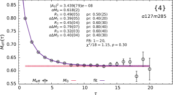
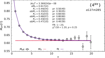
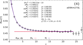
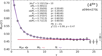
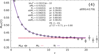
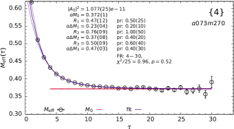
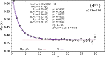
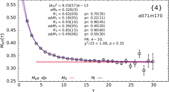
Figure 1: The effective mass $M_{\rm eff}$ plotted versus the source-sink separation $\tau/a$ for 5 ensembles. The left panels show the standard four-state fits, $\{4\}$, while the right panels show $\{4^{N\pi}\}$, in which the noninteracting energy of $N\pi$ state is input as the central value of the prior for $\Delta M_{1}$. The legends give the ground state amplitude ${\mathcal{A}}_{0}$ and mass $aM_{0}$, the excited-state amplitude ratios $R_{i}=|{\mathcal{A}}_{i}|^{2}/|{\mathcal{A}}_{0}|^{2}$ and mass gaps $a\Delta M_{i}=a(M_{i}-M_{i-1})$, the prior value and width (pr) used, the fit range FR, the $\chi^{2}/$dof and the ensemble ID. The signal-to-noise grows rapidly after $\tau=1.8\hbox{--}2.2$ fm depending on the statistics and the ensemble. Note that for the $170$ MeV ensembles, even the ground state mass and amplitude differ by about 2–3$\sigma$ between the two fit strategies, and the relative contribution, $R_{1}e^{-{\Delta M_{1}\tau}}$, of the low mass $N(\bm{1})\pi(-\bm{1})$ state in the $\{4^{N\pi}\}$ fit is still about $3\%$ at $\tau\approx 1.8$ fm.

V The nucleon spectrum from fits to the two-point function

To determine the nucleon spectrum, we keep four states in the spectral decomposition of the two-point functions $C^{2\text{pt}}$ with momentum $\bm{p}$:

$$C^{2\text{pt}}(\tau;\bm{p})=\sum_{i=0}^{3}\lvert\mathcal{A}_{i}(\bm{p})\rvert^{2}e^{-E_{i}(\bm{p})\tau}\,.$$ (15)

Here $E_{i}$ are the energies and ${\mathcal{A}}_{i}$ are the corresponding amplitudes for the creation/annihilation of a given state $|i\rangle$ by the interpolating operator $\cal N$ chosen to be

$$\mathcal{N}(x)=\epsilon^{abc}\left[{q_{1}^{a}}^{T}(x)C\gamma_{5}\frac{(1\pm\gamma_{4})}{2}q_{2}^{b}(x)\right]q_{1}^{c}(x)\,,$$ (16)

with color indices $\{a,b,c\}$, charge conjugation matrix $C=\gamma_{4}\gamma_{2}$ in the DeGrand-Rossi basis DeGrand and Rossi (1990), and $q_{1}$ and $q_{2}$ denoting the two different flavors of light Dirac quarks. The $E_{i}$ and the ${\mathcal{A}}_{i}$ are extracted from a fit to a large range, $[\tau_{\rm min},\tau_{\rm max}]$. The starting time, $\tau_{\rm min}/a$ is taken to be small, between 1 and 4, and $\tau_{\rm max}$ is $\sim 2$ fm with the current statistics as shown in Fig. 1. For brevity, throughout this paper, it should be assumed that the values of $t$ and $\tau$ are in lattice units.

There are two nagging issues with this “standard” analysis. First the mass gaps, $\Delta E_{1}\equiv(E_{1}-E_{0})$, shown in Table 2 are slightly larger than even of N(1440). This could be explained away by assuming that the lower-energy states, such as $N\pi$ or even N(1440), do not couple significantly. Second, the axial vector and pseudoscalar form factors obtained using this spectrum to remove the ESC do not satisfy the PCAC relation, Eq. (4), to a much larger extent than observed in the original three-point correlation functions in which the size of deviation is consistent with that expected due to discretization errors Gupta et al. (2017).

The likely reason for both issues is that standard fits to the two-point function do not expose the lighter multihadron, $N\pi$, $N\pi\pi,\ldots$, states that are needed in the analysis of three-point functions Jang et al. (2020a). In Fig. 1, we show results of four-state fits to $C^{2\text{pt}}(\tau;\bm{p}=0)$ along with the data for the effective energy defined as

$$E_{\rm eff}(\tau)=\log\frac{C^{\rm 2pt}(\tau)}{C^{\rm 2pt}(\tau+1)}\,.$$ (17)

It converges to the ground state energy for $\tau\to\infty$ and for $\bm{p}=0$ reduces to $M_{\rm eff}(\tau)$. The criteria used for judging the quality of the fits is $\chi^{2}$/dof. The panels on the left show fits with the standard strategy labeled $\{4\}$, in which empirical Bayesian priors with wide widths are used only to stabilize the fits. The initial central values for the priors for $\Delta M_{1}\equiv M_{1}-M_{0}$, $\Delta M_{2}\equiv M_{2}-M_{1}$, and for the corresponding amplitude ratios, $R_{i}\equiv|{\mathcal{A}}_{i}|^{2}/|{\mathcal{A}}_{0}|^{2}$, are taken from an unconstrained three-state fit. Prior widths are set at $\sim 50\%$ of the value. The fit is repeated and resulting values are used as central values for the priors in a four-state fit. This process is iterated one more time to adjust the priors for the three excited states. The final fit parameters for the $\bm{p}=0$ case, the prior value and width, the fit range (FR) and the augmented $\chi^{2}$/dof of the fit are given in the labels.

The second strategy, labeled $\{4^{\rm N\pi}\}$, uses a prior for the mass gap, $\Delta E_{1}$, with value given by the lowest relevant state, $N({\bm{1}})\pi(-\bm{1})$ or $N({\bm{0}})\pi({\bm{0}})\pi({\bm{0}})$, with a narrow width. (The priors and their widths for the five larger volume ensembles are given in the labels in Fig. 1.) No narrow prior is put on the amplitude $R_{1}$. The rest of the procedure is the same as for $\{4\}$.

We stress an important clarification regarding the notation $\Delta E_{1}$ and it “representing” the first excited state that is implicit throughout this paper. The value of $\Delta E_{1}$ given by a four-state fit is a number that minimizes $\chi^{2}$/dof and, most likely, represents an “effective” combination of a set of the lowest contributing states. Fits to different correlation functions can, therefore, give different “effective” $\Delta E_{1}$ (in fact $\Delta E_{i}$) depending on the couplings of and spacings between the contributing states.

There are two reasons for stopping at four-state fits. First, in the three-state fits to the three-point functions we use $E_{0}$, $E_{1}$ and $E_{2}$. The ignored $E_{3}$, which is most contaminated by all the higher neglected states, acts as a buffer. Second, including more than four states overparameterizes the fits. A summary of the ground-state mass and the mass gap of the first excited state obtained from different fits is given in Table 2. Note that in most cases, the $a\Delta M_{1}^{\{4\}}$ is a little larger but close to that expected for the N(1440). The one exception is the low value on the $a094m270$ ensemble that should be the same, modulo finite volume corrections, as from $a094m270L$.

ID	$aM_{N}^{\{4\}}$	$aM_{N}^{\{4^{N\pi}\}}$	$a\Delta M_{1}^{\{2\}}$	$a\Delta M_{1}^{\{4\}}$	$a\Delta M_{1}^{\{4^{N\pi}\}}$	$a\Delta{\widetilde{M}}_{1}^{\{2^{\text{free}}\}}|_{g_{A}}$	$a\Delta{\widetilde{M}}_{1}^{\{2^{\text{free}}\}}|_{g_{S}}$	$a\Delta{\widetilde{M}}_{1}^{\{2^{\text{free}}\}}|_{g_{T}}$
$a127m285$	0.618(2)	0.617(2)	0.43(5)	0.39(5)	0.33(2)	0.15(7)	0.71(11)	0.60(10)
$a094m270$	0.468(5)	0.470(2)	0.31(6)	0.22(8)	0.25(1)	0.09(13)	0.51(6)	0.54(3)
$a094m270L$	0.466(1)	0.465(1)	0.35(2)	0.28(5)	0.20(2)	0.13(3)	0.52(2)	0.50(1)
$a091m170$	0.416(2)	0.413(3)	0.34(2)	0.29(5)	0.16(1)	0.08(13)	0.39(8)	0.46(6)
$a091m170L$	0.415(2)	0.408(4)	0.31(3)	0.24(3)	0.14(2)	0.14(9)	0.54(9)	0.44(4)
$a073m270$	0.372(1)	0.372(1)	0.32(2)	0.23(4)	0.20(2)	0.06(3)	0.40(2)	0.40(2)
$a071m170$	0.326(3)	0.323(2)	0.25(3)	0.18(5)	0.12(1)	0.08(4)	0.41(7)	0.38(2)

Table 2: Results for the nucleon mass in lattice units, $aM_{N}^{\{4\}}$ and $aM_{N}^{\{4^{N\pi}\}}$, obtained from the two four-state fits to the two-point functions. The next six columns give the values of the mass gap, $a\Delta M_{1}\equiv a(M_{1}-M_{0})$, of the first excited state obtained from different fits studied in this work. The notation {2} ({4}) denotes a two-state (four-state) fit to the two-point functions, ($\{4^{N\pi}\}$) is a four-state fit to the two-point functions with a prior for $a\Delta M_{1}$ with a narrow width corresponding to the noninteracting $N(\bm{q})\pi(-\bm{q})$ (or the $N(\bm{0})\pi(\bm{0})\pi(\bm{0})$) state (see also Appendix A). In the three $\{2^{\text{free}}\}$ cases, the mass gaps $a\Delta{\widetilde{M}}_{1}$ are determined from fits to the three-point functions used to extract the three charges $g_{A,S,T}$ as explained in Sec. VIII.

We find, illustrated by the zero-momentum case in Fig. 1, that (i) the final value of $\Delta M_{1}^{\rm N\pi}$ tracks the prior in $\{4^{\rm N\pi}\}$ and (ii) the two fits, $\{4\}$ and $\{4^{\rm N\pi}\}$, are not distinguished on the basis of the augmented $\chi^{2}/$dof, which are similar. In fact, for each $\bm{p}$ there is a flat direction in $E_{1}$, i.e., a whole region of parameter values between $\{4\}$ and $\{4^{\rm N\pi}\}$ gives similar augmented $\chi^{2}/$dof. Since the $E_{1}^{\rm N\pi}$ corresponds to roughly the value for the lowest theoretically allowed state and is much smaller than the radial excitation N(1440) or $E_{1}^{\rm 2pt}$, we will assume it is a good estimate of the lower end of possible values. Similarly, the data derived $E_{1}^{\rm 2pt}$ is taken to be an estimate of the upper end when probing the sensitivity of results for the ground state matrix elements to $E_{1}$. Later we will discuss other estimates of $E_{1}$ obtained from fits to the three-point functions.

The values of $Q^{2}={\bm{p}}^{2}-(E-M_{N})^{2}$ for the two strategies are given in Table 17, and are essentially the same. Nevertheless, all the analyses and plots presented use the values of $Q^{2}$ appropriate to the fits, $\{4\}$ or $\{4^{\rm N\pi}\}$.

An important point to note from Fig. 1 is that the $M_{\rm eff}$ data from the $M_{\pi}\approx 170$ MeV ensembles do not show a plateau over the range $1\lesssim\tau\lesssim 2$ fm, in contrast to what is commonly assumed. Concomitantly, we find a systematic difference in $M_{0}$ and ${\mathcal{A}}_{0}$ between the two strategies, $\{4\}$ and $\{4^{\rm N\pi}\}$, with $\{4^{\rm N\pi}\}$ giving a 1–2$\sigma$ smaller value for both $M_{0}$ and $|{\mathcal{A}}_{0}|^{2}$, and the relative difference growing as $M_{\pi}$ is reduced. Note that the correlated decrease in $M_{0}$ and $|{\mathcal{A}}_{0}|^{2}$ under $\{4\}\to\{4^{\rm N\pi}\}$ is consistent with both fits preserving the asymptotic, $\tau\to\infty$, value of $C^{2\text{pt}}(\tau)$. Such a variation implies that one has to re-examine the strategy for even extracting $M_{0}$ in calculations where percent precision is needed, such as in the calculation of the pion-nucleon sigma term, $\sigma_{\pi N}$, using the Hellmann-Feynman theorem Aoki et al. (2020); Gupta et al. (2021) and in the extraction of matrix elements discussed here. Consequently, we consider a number of strategies for the analysis of charges and axial and vector form factors in Sec.s VI, VIII, X and XII.

VI Controlling excited-state contamination in three-point functions

The spectral decomposition of the three-point functions, $C_{\mathcal{O}}^{3\text{pt}}$, truncated at 3 states is:

$$C_{\mathcal{O}}^{3\text{pt}}(\tau;t)=\sum_{i,j=0}^{2}{\mathcal{A}_{i}^{\bm{p}}}{\mathcal{A}_{j}}\langle i^{\bm{p}}\lvert\mathcal{O}\rvert j\rangle e^{-E_{i}t-E_{j}(\tau-t)}\,,$$ (18)

where $O$ is the operator, $\mathcal{A}_{i}$ are the amplitudes with which the states $|i\rangle$ are created by the interpolating operator ${\mathcal{N}}$ with energies $E_{i}$ as defined in Eq. (15). The source point has been translated to $t=0$, the operator is inserted at time $t$, and the nucleon is annihilated at the sink time slice $\tau$. In Eq. (18), $\mathcal{A}_{i}^{\bm{p}}$ and $|i^{\bm{p}}\rangle$ denote that these states could have nonzero momentum $\bm{p}$, whereas the momentum at the sink is fixed to zero in all three-point functions. Thus, for momentum transfer $\bm{q}=\bm{p}$, the initial nucleon’s momentum is $-\bm{p}$.

In principle, the spectrum of the transfer matrix that contributes to the three-point functions, Eq. (18), should be obtainable from the two-point function, Eq. (15), however, the relative contributions can vary significantly as mentioned above, particularly in different 3-point functions. As a result, their contribution may be manifest in some correlators but not in all. This is demonstrated for the axial channel in Sec. IX and for the vector current in Sec. XII.

It is important for the reader to note that individual excited state amplitudes ${\mathcal{A}_{i}^{\bm{p}}}$ and ${\mathcal{A}_{j}}$ with $i,j>0$, and their values determined from fits to two-point functions, $C^{2\text{pt}}(\tau)$, are never used in fits to $C_{\mathcal{O}}^{3\text{pt}}(\tau;t)$. The reason is that in fits to $C_{\mathcal{O}}^{3\text{pt}}(\tau;t)$, only the combinations ${\mathcal{A}_{i}^{\bm{p}}}{\mathcal{A}_{j}}\langle i^{\bm{p}}\lvert\mathcal{O}\rvert j\rangle$ enter. Furthermore, while these combinations are unknown parameters in fits to $C_{\mathcal{O}}^{3\text{pt}}(\tau;t)$ to remove ESC, they are not used any further in the analysis.

Data for the three-point functions have been accumulated for the 4–6 values of $\tau$ specified in Table 15, and for each $\tau$ for all values $0<t<\tau$. In much of the subsequent analyses, we make $3^{\ast}$-state fits. These are three-state fits with the term proportional to $\langle 2^{\bm{p}}\lvert\mathcal{O}\rvert 2\rangle$ set to zero as it is not resolved with the current data and including it overparameterizes the fit.

The spectral decomposition, given in Eqs. (15) and (18), forms the basis of all analyses of excited-state contamination in two- or three-point functions. In order to extract the ground state matrix element $\langle 0^{\bm{p}}\lvert\mathcal{O}_{\Gamma}\rvert 0\rangle$ for a given $\bm{p}$ using the three-state ansatz given in Eq. (18), one has to, a priori, resolve 16 parameters from fits to $C_{\mathcal{O}}^{3\text{pt}}$ calculated as a function of $t$ and $\tau$. These are $\mathcal{A}_{0},\mathcal{A}_{0}^{\bm{p}}$, the three each $M_{i}$ and $E_{i}$, and the eight products of the type $\lvert\mathcal{A}_{0}^{\bm{p}}\rvert\lvert\mathcal{A}_{1}\rvert\langle 0^{\bm{p}}\lvert\mathcal{O}_{\Gamma}\rvert 1\rangle$ involving excited state transition matrix elements. The ideal situation occurs when $\mathcal{A}_{0},\mathcal{A}_{0}^{\bm{p}}$ and the three $M_{i}$ and $E_{i}$ can be obtained from, say, fits to the two-point functions for then the fit ansatz reduces to a sum of terms with a linear dependence on the unknowns. This, however, requires the states that provide significant contributions to two- and three-point functions at the simulated values of $t$ and $\tau$ are the same—naively a reasonable expectation since the same interpolating operator $\cal N$ is used in both.

In Ref. Jang et al. (2020a), we showed that, operationally, this expectation fails for the form factors in the axial vector and pseudoscalar channels. In fact, taking the three $M_{i}$ and $E_{i}$ from $\{4\}$-fits to $C^{2\text{pt}}(\tau;\bm{p})$ to extract the axial vector form factors from $C_{A_{\mu}}^{3\text{pt}}$ and $C_{P}^{3\text{pt}}$ gave results that do not satisfy the PCAC relation between them. Since the original correlation functions, $C_{A_{\mu}}^{3\text{pt}}$ and $C_{P}^{3\text{pt}}$, do satisfy PCAC up to discretization errors, the problem was shown to be introduced while extracting the ground state matrix elements from the correlation functions. We showed that the lower-energy excited states $N(\bm{q})\pi(-\bm{q})$ and $N(\bm{0})\pi(-\bm{q})$ contribute to the two sides of the operator insertion in the three-point functions even though they are not manifest in straightforward fits to the two-point function. The lesson was, one cannot just take the spectrum obtained from the two-point function with current statistics and apply it to all the three-point functions. One has to explore and validate, both numerically and theoretically, the relevant values of $M_{i}$ and $E_{i}$ to use in the extraction of the various ground state matrix elements.

Theoretically, $N(\bm{q})\pi(-\bm{q})$ and $N(\bm{0})\pi(-\bm{q})$ states have much smaller energy, $E_{1}$, compared to that obtained from standard fits to the two-point function. (The noninteracting energies of multiparticle states in a finite box are taken to be the sum of lattice single particle energies assuming a relativistic dispersion relation.) The clue to their relevance came from fits to the three-point function with the insertion of the time component of the axial current, $\langle\Omega|{\mathcal{N}}(\tau)A_{4}(t){\mathcal{N}}(0)|\Omega\rangle$ Jang et al. (2020a). Fits to it using Eq. (18) with the $E_{i}$ from standard fits to $C^{2\text{pt}}(\tau;\bm{p})$ gave large $\chi^{2}/$dof. Consequently these data were ignored in previous works (see Ref. Gupta et al. (2017)) because $G_{A}$ and ${\widetilde{G}}_{P}$ can be determined from the $A_{i}$ correlators as defined in Eqs. (20)–(22), i.e., the $A_{4}$ data were superfluous because the system of equations, Eqs. (20)–(23), is overdetermined. The reason for the poor signal was that the ESC in this channel is very large, in fact it dominates the signal. Exploiting this last fact led us to determine the relevant mass gap[s], which are much smaller than the standard $\Delta E_{1}$, i.e., from $\{4\}$.

To analyze $\langle\Omega|{\mathcal{N}}(\tau)A_{4}(t){\mathcal{N}}(0)|\Omega\rangle$ we, instead, used the two-state version of Eq. (18) with the excited state energy $E_{1}$ left as a free parameter Jang et al. (2020a). The resulting value, labeled $E_{1}^{\rm A4}$, was close to the noninteracting $N\pi$ state, and much smaller than what the fits to the two-point function gave (labeled $E_{1}^{\rm 2pt}$). The three form factors $G_{A}$, ${G}_{P}$ and ${\widetilde{G}}_{P}$, extracted using $E_{1}^{\rm A4}$, satisfied PCAC to within expected lattice systematics. This resolution has, however, created a conundrum for the analysis of all nucleon matrix elements—what are the relevant excited-state energies, $E_{i}$, that contribute to a given matrix element, how to determine them, and how to deal with the towers of multiparticle states such as $N\pi$, $N\pi\pi$, $\cdots$ that have the same quantum numbers as the nucleon and become increasingly dense as the lattice size $L\to\infty$. Addressing these questions is particularly hard for channels that do not have an independent check such as PCAC.

The tools available include extracting the $E_{i}$ from fits to the three-point functions themselves, getting guidance from heavy baryon chiral perturbation theory, evaluating the full tower of excited states that could contribute, and satisfying relations such as PCAC. In this paper, we attempt to develop a framework to determine the relevant $E_{i}$ for each matrix element considered and, if possible, associate them with [multi]hadron states for a deeper understanding of the excited states that contribute. For the axial channel, this is done in Appendix E, and for the vector channel in Sec. XII

Throughout the paper, we will use $M_{i}$ and $E_{i}$ for first excited-state energies determined from four-state fits to the two-point functions, and ${\widetilde{M}}_{1}$ and ${\widetilde{E}}_{1}$ for the values obtained from two-state fits to the three-point functions.

VII Extracting form factors from ground state matrix elements

All matrix elements are obtained from fits to the three-point correlators with the insertion of the various components of the axial, pseudoscalar, scalar, tensor and vector currents. To display these three-point correlator data we construct the ratio, ${\cal R}_{\mathcal{O}}$, of the three-point to the two-point correlation functions,

$${\cal R}_{\mathcal{O}} (t,\tau,\bm{p},\bm{0})=\frac{C^{3\text{pt}}_{\mathcal{O}}(t,\tau;\bm{p},\bm{0})}{C^{2\text{pt}}(\tau,\bm{p})}\,\times\,$$

$$\left[\frac{C^{2\text{pt}}(t,\bm{p})C^{2\text{pt}}(\tau,\bm{p})C^{2\text{pt}}(\tau-t,\bm{0})}{C^{2\text{pt}}(t,\bm{0})C^{2\text{pt}}(\tau,\bm{0})C^{2\text{pt}}(\tau-t,\bm{p})}\right]^{1/2}\,,$$ (19)

where $C^{2\text{pt}}$ and $C_{\mathcal{O}}^{3\text{pt}}$ are defined in Eqs. (15) and (18). This ratio gives the desired ground state matrix element in the limits $t\to\infty$ and $(\tau-t)\to\infty$. For all the two-point correlation functions in Eq. (19), we use the results of the appropriate four-state fit instead of the measured values. When calculating the three-point correlation functions, we use the spin projection ${\cal P}=(1+\gamma_{4})(1+i\gamma_{5}\gamma_{3})/2$. As a result, the “3” direction is special while “1” and “2” are equivalent under the rotational cubic symmetry. For the axial vector current, $\overline{q}\gamma_{5}\gamma_{\mu}q$, the imaginary part of the $A_{i}$ and real part of $A_{4}$ have a signal in the following four ratios and give the desired form factors in the limit $t$ and $(\tau-t)\to\infty$:

$${\cal R}_{51}\rightarrow \;\frac{1}{\sqrt{(2E_{p}(E_{p}+M))}}\left[-\frac{q_{1}q_{3}}{2M}{\widetilde{G}}_{P}\right]\,,$$ (20)

$${\cal R}_{52}\rightarrow \;\frac{1}{\sqrt{(2E_{p}(E_{p}+M))}}\left[-\frac{q_{2}q_{3}}{2M}{\widetilde{G}}_{P}\right]\,,$$ (21)

$${\cal R}_{53}\rightarrow \;\frac{1}{\sqrt{(2E_{p}(E_{p}+M))}}\left[-\frac{q_{3}^{2}}{2M}{\widetilde{G}}_{P}+(M+E)G_{A}\right]\,,$$ (22)

$${\cal R}_{54}\rightarrow \;\frac{q_{3}}{\sqrt{(2E_{p}(E_{p}+M))}}\left[\frac{M-E}{2M}{\widetilde{G}}_{P}+G_{A}\right]\,.$$ (23)

The ${\widetilde{G}}_{P}$ can be determined from ${\cal R}_{51}$ with momenta $\bm{q}=(i,0,j)\times(2\pi/La)$ and from ${\cal R}_{52}$ with $\bm{q}=(0,i,j)\times(2\pi/La)$. In practice, cases equivalent under the cubic symmetry are averaged before we make the ESC fits. The $G_{A}$ can be determined uniquely from ${\cal R}_{53}$ with $q_{3}=0$. In the other momentum channels, the coupled set of equations, Eqs. (20)–(22), are solved for $G_{A}$ and ${\widetilde{G}}_{P}$ using the full covariance matrix. The $A_{4}$ correlator gives a second, and so far considered redundant because of the much larger errors, linear combination of $G_{A}$ and ${\widetilde{G}}_{P}$. As discussed below, it will play an important role in determining the first excited state parameters, and thus in the overall analysis.

The pseudoscalar form factor $G_{P}(Q^{2})$ is given by the real part of ${\cal R}_{5}$, i.e., with $\mathcal{O}=\overline{q}{\gamma_{5}}q$ in Eq. (19):

$${\cal R}_{5}\rightarrow \;\frac{1}{\sqrt{(2E_{p}(E_{p}+M))}}\left[q_{3}{G}_{P}\right]\,.$$ (24)

For the electric and magnetic form factors, the following quantities, with $\mathcal{O}=(2\overline{u}\gamma_{\mu}u-\overline{d}\gamma_{\mu}d)/3$, have a signal:

$$\sqrt{2E_{p}(M_{N}+E_{p})}\,\Re({\cal R}_{i})= \;-\epsilon_{ij3}q_{j}{G}_{M}\,,$$ (25)

$$\sqrt{2E_{p}(M_{N}+E_{p})}\,\Im({\cal R}_{i})= \;q_{i}{G}_{E}\,,$$ (26)

$$\sqrt{2E_{p}(M_{N}+E_{p})}\,\Re({\cal R}_{4})= \;(M_{N}+E_{p}){G}_{E}\,.$$ (27)

Exploiting the cubic symmetry under spatial rotations, we construct two averages over equivalent three-point correlators before doing fits to get the ground-state matrix elements: over $\Re({C}_{1}^{\rm 3pt})$ and $\Re({C}_{2}^{\rm 3pt})$ for $G_{M}(Q^{2})$ and over $\Im({C}_{1}^{\rm 3pt})$, $\Im({C}_{2}^{\rm 3pt})$ and $\Im({C}_{3}^{\rm 3pt})$ for $G_{E}(Q^{2})$. We label these form factors as $G_{M}^{V_{i}}$ and $G_{E}^{V_{i}}$. Together with $G_{E}^{V_{4}}$ extracted from Eq. (27), they constitute the three form factors analyzed. Each is obtained from a distinct correlation function, and it is important to note that the discretization artifacts and the excited-state contaminations in these can be very different.

We remind the reader that these ratios are used only to plot the data. Our results are obtained by making $n$-state fits to the correlation functions themselves. In making these fits we attempt to balance statistical and systematic uncertainties. Data at smaller $\tau$ have smaller statistical errors but larger ESC because a larger number of states contribute. Similarly, data close to the source and the sink have larger ESC. Therefore, for each $\tau$ we neglect data on $t_{\rm skip}$ time slices at either end, and we make fits to data with the largest $\tau$ values that have statistically precise data. By skipping the same number of points, $t_{\rm skip}$, at all $\tau$ fit, we increase the weight of the larger $\tau$ data to partially compensate for the larger statistical weight given to the lower error points at smaller $\tau$.

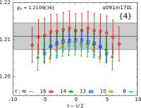
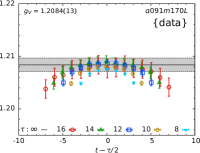
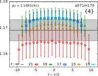
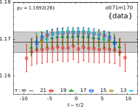
Figure 2: Data for the ratio $R_{V_{4}}$, which give $g_{V}$ in the limit $\tau\to\infty$, are plotted versus $t-\tau/2$ for the $a091m170L$ (left two) and $a071m170$ (right two) ensembles. Panels 1 and 3 show results using the $\{4\}$-state fit for $C^{\rm 2pt}$ in $R_{V_{4}}$, while in panels 2 and 4 the data for $C^{\rm 2pt}$ are used. The final estimate shown by the gray band is the average of the five (six) central points for $\tau=14,16$ ($\tau=19,21$) for the $a091m170L$ ($a071m170$) ensemble.

VIII Extracting nucleon charges

This section covers the calculations of the isovector nucleon charges, $g_{\Gamma}^{u-d}$, from the forward matrix elements:

$$\langle N(p,s)|\mathcal{O}_{\Gamma}|N(p,s)\rangle=g_{\Gamma}\bar{u}_{s}(p)\Gamma u_{s}(p)\,.$$ (28)

For $\bm{q}=0$ in the three-point functions, Eq. (19) simplifies to ${\cal R}_{\mathcal{O}_{\Gamma}}(t,\tau,\bm{0},\bm{0})=C^{3\text{pt}}_{\mathcal{O}_{\Gamma}}(t,\tau;\bm{0},\bm{0})/C^{2\text{pt}}(\tau,\bm{0})$. With the spin projection in the “3” direction, the Dirac matrix structure of operators used to calculate the scalar, vector, axial and tensor charges are $\Gamma=1,\gamma_{4},\gamma_{3}\gamma_{5}$ and $\sigma_{12}$, respectively. Since the nucleon states and all four operators, which commute with $\gamma_{4}$, have positive parity, therefore all possible excited states with positive parity are theoretically allowed in all four channels: axial, scalar, tensor and vector. Based on conserved symmetries alone, the ones with the smallest mass gap are $N(0)\pi(0)\pi(0)$ or $N({\bm{1}})\pi(-{\bm{1}})$. As mentioned above, their noninteracting energies are roughly the same on each of the seven ensembles. The unknown is their coupling in the various channels. Furthermore, the analysis of the two-point function in Sec. V showed that there is a large range of $M_{1}$ values with similar $\chi^{2}$/dof in four-state fits. This range includes the $N\pi$ and $N\pi\pi$ states. We will, therefore, investigate the impact on ground state matrix elements of choosing values of $M_{1}$ over this interval, the lower end of which is taken to be the approximately degenerate energy of these two states ignoring interactions.

The question is how to determine, nonperturbatively, which of the possible states contribute significantly? In chiral perturbation theory, $N({\bm{1}})\pi(-{\bm{1}})$ arises at one-loop Bär, Oliver (2016) and $N(0)\pi(0)\pi(0)$ at two loops Bär, O. (2018) in the axial channel. Similarly, the vector current couples to the $\rho$ meson (vector meson dominance), or equivalently the two-pion state it decays into for sufficiently small pion mass (see also the discussion in Ref. Hoferichter et al. (2016)). As will be shown later, the contribution of these multihadron states increases with decreasing $M_{\pi}$ (and $\bm{q}$ in the case of form factors) in both the axial and the vector channels. More generally, it is, a priori, not straightforward to narrow down the states that give significant contributions to a particular correlation function. Again, the criterion we will use is the $\chi^{2}/$dof of the fits, input from $\chi$PT, and the sensitivity of the observables to the value of the mass gaps used in the fit to judge the best strategy.

To include the effect of either of the two kinds of states, $N(0)\pi(0)\pi(0)$ or $N({\bm{1}})\pi(-{\bm{1}})$, we use the spectrum from the $\{4^{N\pi}\}$ fit noting that the fit to the three-point function only cares about $\Delta M_{1}$ and not the identity of the state[s]. So, in the current analysis, the contributions from all three possibilities, $N(0)\pi(0)\pi(0)$ or $N({\bm{1}})\pi(-{\bm{1}})$ or both, are included under the same label $\{4^{N\pi}\}$.

We examine two more strategies, which we call $\{4,2^{\rm free}\}$ and $\{4^{N\pi},2^{\rm free}\}$, in which $E_{1}$ is left a free parameter to be fixed by a two-state fit to the three-point functions. Note that these two strategies differ only in the ground state parameters ${\mathcal{A}}_{0}$ and $M_{0}$ (or $E_{0}$), which are slightly different between the $\{4^{N\pi}\}$ and $\{4\}$ fits as shown in Fig. 1.

Furthermore, in Appendix D, we examine the ESC in each charge from operator insertion on the $u$ and $d$ quarks separately. These data provide additional understanding of the statistical precision of the data, and how the errors and ESC in the isovector ($u-d$) and in the connected part of the isoscalar ($u+d$) combinations, arise.

Ensemble ID	$g_{V}$	$Z_{V}$	$Z_{V}g_{V}$	$Z_{A}$	$Z_{S}$	$Z_{T}$	$Z_{A}/Z_{V}$	$Z_{S}/Z_{V}$	$Z_{T}/Z_{V}$
$a127m285$	1.260(04)	0.806(23)	1.016(30)	0.882(13)	0.829(15)	0.892(16)	1.089(14)	1.017(40)	1.106(11)
$a094m270$	1.213(05)	0.828(17)	1.005(21)	0.883(12)	0.789(11)	0.928(17)	1.065(09)	0.946(25)	1.121(08)
$a094m270L$	1.203(02)	0.829(19)	0.997(23)	0.886(14)	0.796(14)	0.929(19)	1.070(10)	0.958(29)	1.122(09)
$a091m170$	1.210(03)	0.832(20)	1.006(24)	0.882(13)	0.790(15)	0.931(20)	1.061(11)	0.947(27)	1.122(08)
$a091m170L$	1.211(04)	0.827(18)	1.001(22)	0.875(14)	0.783(11)	0.926(15)	1.056(09)	0.943(24)	1.120(08)
$a073m270$	1.171(02)	0.857(15)	1.003(17)	0.899(11)	0.779(10)	0.961(18)	1.052(09)	0.911(30)	1.124(07)
$a071m170$	1.169(04)	0.853(13)	0.998(16)	0.896(07)	0.767(13)	0.965(15)	1.051(09)	0.897(28)	1.132(07)

Table 3: Results for the bare vector charge $g_{V}$ and the renormalization constants $Z_{A,S,T,V}$ calculated nonperturbatively on the lattice using the RI-sMOM scheme. The value of the product $Z_{V}g_{V}$ is consistent with unity and the errors in it are dominated by those in $Z_{V}$. Note that the errors in the ratios $Z_{A}/Z_{V}$ and $Z_{T}/Z_{V}$ are smaller than those in $Z_{A}$ and $Z_{T}$, respectively, while those in $Z_{S}/Z_{V}$ are larger than in $Z_{S}$.

A comparison between fits with these four strategies is shown in Figs. 17, 18 and 19 for the three charges $g_{A,S,T}$. The data show the following common features:

• The symmetry of $R_{\mathcal{O}}^{\rm 3pt}$ (and $C_{\mathcal{O}}^{\rm 3pt}$) about the midpoint of the interval, $t=\tau/2$, improves with statistics as expected. The observed deviations, mostly in the largest $\tau$ data for $g_{S}$, are statistical fluctuations (see also the discussion in Appendix D).

• The value of $R_{\mathcal{O}}^{\rm 3pt}$ at each $t$ (especially at the midpoint, $t=\tau/2$) converges monotonically toward the $\tau=\infty$ value. Having a clear monotonic behavior, i.e., not obscured by the errors, is important for choosing the values of $\tau$ to keep in the $n$-state fits to remove ESC, and it improves the stability of the fits with respect to variations in $\tau$ and $t_{\rm skip}$. .

Having data with these features, hallmarks of high statistics calculations, improves the reliability of three-state fits that we make to the largest three (four) values of $\tau$ listed in Table 15 to obtain results in the limit $\tau\to\infty$ for $g_{A}$ and $g_{T}$ ($g_{S}$). To evaluate the convergence of estimates for $g_{A,S,T}$ on each ensemble, we compared results from the two- and $3^{\ast}$-state fits. Using this framework, and the methodology for statistical analysis given in Sec. III, the four charges, $g_{A,S,T,V}$, are analyzed next.

VIII.1 $g_{V}$ and Operator Renormalization

The data for the vector charge obtained from the correlator $\langle N(\tau,{\bm{0}})V_{4}(t,{\bm{0}})N(0,{\bm{0}})\rangle$ show a small (about 1%) variation over the range of $\tau$ values investigated as illustrated in Fig. 2 for the $a091m170L$ and $a071m170$ ensembles. We show two versions of the ratio ${\cal R}_{V}(t,\tau,0,0)$: $C^{3\text{pt}}_{V}(t,\tau;\bm{0},\bm{0})/C^{2\text{pt}}(\tau,\bm{0})|_{\rm fit}$ and $C^{3\text{pt}}_{V}(t,\tau;\bm{0},\bm{0})/C^{2\text{pt}}(\tau,\bm{0})$, where in the first case we use the result of the $\{4\}$ fit, $C^{2\text{pt}}(\tau,\bm{0})|_{\rm fit}$, while in the second case we use the two-point function itself. In both cases, the data are essentially flat about $\tau/2$, so for the final value of $g_{V}$, we take the average of 5–6 central points at the largest two values of $\tau$ using the first version. The errors in these estimates cover the spread in the values at $\tau/2$ for the various $\tau$.

A check on these estimates of $g_{V}$ is that the product $Z_{V}g_{V}=1$ within $O(a)$ discretization errors, where $Z_{V}$ is the renormalization constant for the local vector current used in this study. Values of $Z_{V}g_{V}$ are shown in Table 3 and deviate from unity by $\lesssim 1\%$, i.e., by an amount smaller than the errors in the product that come mainly from $Z_{V}$.

The calculation of the renormalization constants $Z_{A,S,T,V}$ for the local axial, scalar, tensor and vector quark bilinear operators on the lattice is done using the regularization independent symmetric momentum (RI-sMOM) scheme Martinelli et al. (1995); Sturm et al. (2009). Results are then converted to the $\overline{MS}$ scheme at scale 2 GeV using two-loop matching and three-loop running as described in Ref. Yoon et al. (2017). The calculation is done on all seven ensembles. Using these estimates, together with the conserved vector charge relation $Z_{V}g_{V}=1$, we present renormalized quantities calculated in two ways. In the first method, labeled ${\rm Z}_{1}$, the renormalized results for operator $O$ are given by $Z_{O}O$. In the second method, labeled ${\rm Z}_{2}$, we construct the two ratios: $Z_{O}/Z_{V}$ and $g_{O}/g_{V}$ for the charges. For constructing $Z_{O}/Z_{V}$, we start with the ratio of the two amputated three-point functions in the RI-sMOM scheme, and for $g_{O}/g_{V}$, the ratio of the matrix element after making the excited-state fits for each. In both cases, these ratios are taken within the jackknife process. For $Z_{2}$, the expectation is a cancellation of correlated fluctuations in each of the two ratios leading to smaller overall errors. The data summarized in Table 3 show that the errors in $Z_{A}/Z_{V}$ and $Z_{T}/Z_{V}$ are smaller than in $Z_{A,T}$ but not in $Z_{S}/Z_{V}$ versus $Z_{S}$. Furthermore, data in Tables 4 and 5 show smaller errors from ${\rm Z}_{2}$ for $g_{A,T}$ and from ${\rm Z}_{1}$ for $g_{S}$. Results from the two methods, after the CCFV fits carried out in Sec. XIII.1, differ by $\sim 0.03$. When quoting the central values, we will choose to renormalize $g_{A,T}$ using ${\rm Z}_{2}$ and $g_{S}$ using ${\rm Z}_{1}$. The difference between the two estimates will be used to assign an appropriate systematic uncertainty in the three charges.

VIII.2 $g_{A}$

The findings from the four fit strategies, $\{4,3^{\ast}\}$, $\{4^{N\pi},3^{\ast}\}$ (and their two-state versions $\{4,2\}$, $\{4^{N\pi},2\}$ to check for overparameterization), $\{4,2^{\rm free}\}$ and $\{4^{N\pi},2^{\rm free}\}$ are the following:

• The results from the $\{4,2^{\rm free}\}$ or $\{4^{N\pi},2^{\rm free}\}$ fits are shown in Fig. 17 by the broad gray bands and given in the labels. The output values of $\Delta{\widetilde{M}}_{1}$ on all but the $a091m170L$ ensemble have large errors and are much smaller than even those for the $N\pi$ state as shown in Table 2. The reason is that the fluctuations between the jackknife samples are unreasonably large. Lacking statistical control, we do not consider these two strategies any further for $g_{A}$. In future higher precision calculations, especially on $M_{\pi}\lesssim 200$ MeV ensembles, we will continue to check whether estimates from the $\{4,2^{\rm free}\}$ and $\{4^{N\pi},2^{\rm free}\}$ strategies become more robust.

• Overall, two- and $3^{\ast}$-state fits, irrespective of whether inputs of ground state parameters are from either the $\{4\}$ or the $\{4^{N\pi}\}$ fits to two-point functions, overlap on every ensemble. The 3*-state fits are overparameterized with respect to the two-state fits based on both the Akaike criteria and because the uncertainty in the two additional fit parameters is $>100\%$ for the following ensembles and strategies:

  • $a094m270$: $\{4,3^{\ast}\}$, $\{4^{N\pi},3^{\ast}\}$

  • $a091m170$: $\{4^{N\pi},3^{\ast}\}$

  • $a091m170L$: $\{4,3^{\ast}\}$, $\{4^{N\pi},3^{\ast}\}$

  The values from $\{4^{N\pi},3^{\ast}\}$ agree with those from $\{4^{N\pi},2\}$ but have larger errors. To be conservative, we choose the $\{4^{N\pi},3^{\ast}\}$ results for all ensembles.

• There is a roughly $2\sigma$ difference between $\{4,3^{\ast}\}$ and $\{4^{N\pi},3^{\ast}\}$ results on the $M_{\pi}\approx 170$ MeV ensembles, $a091m170$, $a091m170L$ and $a071m170$, as shown in Fig. 3. The $\{4^{N\pi},3^{\ast}\}$ values are larger—a smaller mass gap implies a larger ESC and leads to a larger $\tau\to\infty$ value since the convergence is from below as shown in Fig. 17. The difference is approximately $6\%$ at $M_{\pi}=170$ MeV, and becomes $\approx 8\%$ after the CCFV fits as shown in Table 10 in Sec. XIII.

• A similar difference of approximately $5\%$ is also present in the axial form factor $G_{A}$ for the lowest nonzero momentum transfer, ${\vec{q}}=(1,0,0)2\pi/La$, data on the $M_{\pi}\approx 170$ MeV ensembles between the $\{4,3^{\ast}\}$ and $\{4^{N\pi},3^{\ast}\}$ strategies as shown in Table 18.

The key issue to settle is whether the $N(1)\pi(-1)$ state, which is seen to contribute to the axial form factors at the lowest $Q^{2}$ and whose effect grows as $Q^{2}\to 0$, also contributes at the approximately $5\%$ level to the forward matrix element as indicated by the data. We discuss this issue further in Sec. X, and in Sec. XIII.1 where we compare these estimates of $g_{A}$ to the second set of values obtained by extrapolating $G_{A}(Q^{2})$ to $Q^{2}=0$ using the dipole, Padé and $z$-expansion fits defined in Sec. X.1.

Figure 3: The difference in the renormalized (${\rm Z}_{1}$ method) axial (top), scalar (middle) and the tensor (bottom) charges between the two strategies, $\{4^{N\pi},3^{\ast}\}-\{4,3^{\ast}\}$. The data are shown for all the seven ensembles.

fit	$g_{A}^{\text{bare}}|_{{\bm{q}}=0}$	$g_{A}|_{{\bm{q}}=0}^{{\rm Z}_{1}}$	$g_{A}|_{{\bm{q}}=0}^{{\rm Z}_{2}}$	$g_{A}^{\text{bare}}|_{\text{dipole}}$	$g_{A}^{\text{bare}}|_{P_{2}}$	$g_{A}^{\text{bare}}|_{z^{2}}$	$g_{A}|_{z^{2}}^{{\rm Z}_{1}}$	$g_{A}|_{z^{2}}^{{\rm Z}_{2}}$
$a127m285$
$\{4,3^{\ast}\}$	1.433(13)	1.264(22)	1.238(19)	1.424(13)	1.423(14)	1.424(13)	1.255(21)	1.230(19)
$\{4^{N\pi},3^{\ast}\}$	1.445(13)	1.274(22)	1.248(19)	1.449(16)	1.459(19)	1.453(16)	1.281(23)	1.255(21)
$\{4^{N\pi},2^{A_{4}}\}$	-	-	-	1.458(18)	1.488(26)	1.465(20)	1.291(25)	1.266(23)
$\{4^{N\pi},2^{\text{sim}}\}$	-	-	-	1.429(20)	1.432(32)	1.421(22)	1.252(26)	1.227(24)
$a094m270$
$\{4,3^{\ast}\}$	1.431(51)	1.263(48)	1.256(45)	1.360(27)	1.390(52)	1.386(33)	1.224(34)	1.216(30)
$\{4^{N\pi},3^{\ast}\}$	1.416(21)	1.250(25)	1.242(20)	1.365(25)	1.426(42)	1.409(28)	1.244(30)	1.237(27)
$\{4^{N\pi},2^{A_{4}}\}$	-	-	-
$\{4^{N\pi},2^{\text{sim}}\}$	-	-	-	1.350(25)	1.379(49)	1.375(33)	1.213(33)	1.206(31)
$a094m270L$
$\{4,3^{\ast}\}$	1.3892(96)	1.231(21)	1.236(14)	1.387(9)	1.393(10)	1.392(9)	1.234(21)	1.239(14)
$\{4^{N\pi},3^{\ast}\}$	1.413(11)	1.252(22)	1.258(15)	1.410(13)	1.424(15)	1.418(14)	1.256(23)	1.262(16)
$\{4^{N\pi},2^{A_{4}}\}$	-	-	-	1.412(10)	1.434(13)	1.426(11)	1.264(22)	1.269(15)
$\{4^{N\pi},2^{\text{sim}}\}$	-	-	-	1.397(12)	1.414(17)	1.406(14)	1.246(23)	1.251(17)
$a091m170$
$\{4,3^{\ast}\}$	1.419(20)	1.251(25)	1.244(21)	1.399(15)	1.402(19)	1.413(19)	1.247(25)	1.240(21)
$\{4^{N\pi},3^{\ast}\}$	1.495(41)	1.319(41)	1.311(38)	1.480(40)	1.469(58)	1.488(51)	1.313(49)	1.305(47)
$\{4^{N\pi},2^{A_{4}}\}$	-	-	-	1.412(21)	1.504(36)	1.504(31)	1.327(34)	1.319(31)
$\{4^{N\pi},2^{\text{sim}}\}$	-	-	-	1.421(25)	1.442(41)	1.451(37)	1.280(38)	1.273(35)
$a091m170L$
$\{4,3^{\ast}\}$	1.436(17)	1.257(25)	1.252(19)	1.426(17)	1.419(18)	1.423(19)	1.245(25)	1.241(20)
$\{4^{N\pi},3^{\ast}\}$	1.521(41)	1.331(42)	1.327(39)	1.502(44)	1.487(51)	1.496(49)	1.309(47)	1.305(45)
$\{4^{N\pi},2^{A_{4}}\}$	-	-	-	1.441(25)	1.507(32)	1.504(30)	1.316(33)	1.312(29)
$\{4^{N\pi},2^{\text{sim}}\}$	-	-	-	1.499(27)	1.538(36)	1.536(33)	1.344(36)	1.339(32)
$a073m270$
$\{4,3^{\ast}\}$	1.371(15)	1.233(20)	1.232(17)	1.358(11)	1.359(17)	1.363(14)	1.226(19)	1.226(16)
$\{4^{N\pi},3^{\ast}\}$	1.384(12)	1.245(18)	1.244(15)	1.361(11)	1.402(18)	1.392(13)	1.251(19)	1.251(16)
$\{4^{N\pi},2^{A_{4}}\}$	-	-	-	1.329(12)	1.359(18)	1.348(14)	1.212(20)	1.212(16)
$\{4^{N\pi},2^{\text{sim}}\}$	-	-	-	1.342(12)	1.365(19)	1.360(15)	1.222(20)	1.222(17)
$a071m170$
$\{4,3^{\ast}\}$	1.414(34)	1.267(32)	1.271(33)	1.371(21)	1.372(23)	1.377(24)	1.234(24)	1.237(24)
$\{4^{N\pi},3^{\ast}\}$	1.479(38)	1.325(36)	1.329(36)	1.448(37)	1.476(49)	1.484(46)	1.329(42)	1.333(43)
$\{4^{N\pi},2^{A_{4}}\}$	-	-	-	1.359(21)	1.469(32)	1.472(30)	1.319(29)	1.323(29)
$\{4^{N\pi},2^{\text{sim}}\}$	-	-	-	1.432(29)	1.483(44)	1.485(40)	1.330(37)	1.334(38)

Table 4: Results for $g_{A}$ from the seven ensembles and with the four strategies, specified in column one and defined in Appendix A, used to control the excited state contamination. The second column gives estimates from the forward matrix element ($q=0)$ for the two strategies $\{4,3^{\ast}\}$ and $\{4^{N\pi},3^{\ast}\}$ in which the excited state spectrum is taken from $\{4\}$ and $\{4^{N\pi}\}$ fits to ${\cal C}^{\rm 2pt}$. Columns 5–7 give $g_{A}$ obtained by extrapolating $G_{A}(Q^{2}\neq 0)$ data using a dipole, $P_{2}$ Padé and $z^{2}$ fits to all ten $Q^{2}\neq 0$ points. The fits to $\{4^{N\pi},2^{A_{4}}\}$ data on the $a094m270$ ensemble are not stable, so no results are presented. The corresponding renormalized values using the two methods, ${\rm Z}_{1}\equiv Z_{A}g_{A}^{\rm bare}$ and ${\rm Z}_{2}\equiv(Z_{A}/Z_{V})\times(g_{A}^{\rm bare}/g_{V}^{\rm bare})$, are given in columns 3-4 and 8-9.

fit	$g_{S}^{\text{bare}}$	$g_{S}|^{{\rm Z}_{1}}$	$g_{S}|^{{\rm Z}_{2}}$	$g_{T}^{\text{bare}}$	$g_{T}|^{{\rm Z}_{1}}$	$g_{T}|^{{\rm Z}_{2}}$
$a127m285$
{4,3*}	1.083(27)[0.94]	0.897(28)	0.874(41)	1.173(10)[1.16]	1.046(21)	1.029(14)
{$4^{N\pi}$,3*}	1.091(31)[0.96]	0.904(30)	0.880(43)	1.169(12)[1.18]	1.043(22)	1.026(15)
{$4,2^{\text{free}}$}	1.036(22)[1.16]	0.858(24)	0.836(37)	1.1825(83)[1.10]	1.055(20)	1.038(13)
{$4^{N\pi},2^{\text{free}}$}	1.041(21)[1.15]	0.863(23)	0.840(37)	1.1839(92)[1.16]	1.056(21)	1.039(13)
$a094m270$
{4,3*}	1.22(10)[1.21]	0.965(83)	0.953(84)	1.102(24)[1.12]	1.022(30)	1.019(24)
{$4^{N\pi}$,3*}	1.193(58)[1.22]	0.942(48)	0.930(51)	1.108(19)[1.12]	1.028(26)	1.024(19)
{$4,2^{\text{free}}$}	1.113(48)[1.19]	0.878(40)	0.867(44)	1.140(25)[1.02]	1.058(31)	1.054(24)
{$4^{N\pi},2^{\text{free}}$}	1.101(36)[1.21]	0.869(31)	0.858(36)	1.133(10)[1.01]	1.051(22)	1.047(12)
$a094m270L$
{4,3*}	1.195(24)[1.35]	0.951(25)	0.952(35)	1.0923(86)[0.96]	1.015(22)	1.019(11)
{$4^{N\pi}$,3*}	1.176(43)[1.33]	0.936(38)	0.937(44)	1.095(13)[0.94]	1.017(24)	1.021(15)
{$4,2^{\text{free}}$}	1.165(15)[1.44]	0.927(20)	0.928(30)	1.1110(41)[1.03]	1.032(22)	1.0364(92)
{$4^{N\pi},2^{\text{free}}$}	1.178(15)[1.44]	0.938(20)	0.939(31)	1.1184(47)[1.11]	1.039(22)	1.0433(96)
$a091m170$
{4,3*}	1.172(60)[0.96]	0.926(51)	0.918(54)	1.054(14)[0.84]	0.981(25)	0.977(15)
{$4^{N\pi}$,3*}	1.18(14)[0.95]	0.93(11)	0.92(11)	1.063(39)[0.89]	0.990(42)	0.985(37)
{$4,2^{\text{free}}$}	1.152(53)[0.98]	0.910(45)	0.902(48)	1.083(12)[0.88]	1.009(24)	1.004(13)
{$4^{N\pi},2^{\text{free}}$}	1.188(53)[1.00]	0.938(45)	0.930(49)	1.107(16)[0.88]	1.031(27)	1.027(17)
$a091m170L$
{4,3*}	1.145(73)[0.84]	0.897(58)	0.892(60)	1.061(14)[0.96]	0.983(20)	0.982(15)
{$4^{N\pi}$,3*}	1.17(14)[0.85]	0.92(11)	0.91(11)	1.031(32)[1.01]	0.955(34)	0.954(31)
{$4,2^{\text{free}}$}	1.132(43)[0.91]	0.887(36)	0.882(40)	1.0977(91)[1.04]	1.017(18)	1.016(11)
{$4^{N\pi},2^{\text{free}}$}	1.223(57)[0.95]	0.958(47)	0.952(50)	1.149(26)[1.75]	1.064(29)	1.063(25)
$a073m270$
{4,3*}	1.271(25)[1.13]	0.989(23)	0.989(37)	1.0627(73)[0.87]	1.021(21)	1.0201(91)
{$4^{N\pi}$,3*}	1.272(30)[1.09]	0.990(26)	0.989(40)	1.0623(86)[0.88]	1.020(21)	1.020(10)
{$4,2^{\text{free}}$}	1.230(14)[1.00]	0.958(16)	0.957(33)	1.0823(51)[1.00]	1.040(21)	1.0389(78)
{$4^{N\pi},2^{\text{free}}$}	1.235(14)[1.00]	0.962(16)	0.961(33)	1.0853(46)[1.01]	1.042(20)	1.0418(76)
$a071m170$
{4,3*}	1.22(13)[0.84]	0.94(10)	0.94(10)	1.016(22)[0.92]	0.980(26)	0.983(22)
{$4^{N\pi}$,3*}	1.24(21)[0.84]	0.95(16)	0.95(16)	1.006(34)[0.89]	0.971(36)	0.974(33)
{$4,2^{\text{free}}$}	1.182(72)[0.83]	0.907(57)	0.907(62)	1.052(15)[0.89]	1.016(21)	1.019(16)
{$4^{N\pi},2^{\text{free}}$}	1.230(72)[0.83]	0.943(57)	0.944(62)	1.083(17)[0.96]	1.045(23)	1.049(18)

Table 5: Results for $g_{S}$ and $g_{T}$ on the seven ensembles and for the four strategies specified in column 1 and defined in Appendix A that are used to control the excited state contamination. The second and fifth columns give the bare values. The renormalized values using the two different methods, ${\rm Z}_{1}\equiv Z_{S,T}g_{S,T}^{\rm bare}$ and ${\rm Z}_{2}\equiv(Z_{S,T}/Z_{V})\times(g_{S,T}^{\rm bare}/g_{V}^{\rm bare})$, are given in columns 3–4 and 6–7. The numbers within square brackets give the $\chi^{2}/$dof of the ESC fits.

VIII.3 $g_{S}$

The data and fits to the largest four values of $\tau$ used to remove ESC in $g_{S}$ are shown in Fig. 18. The statistical errors in individual points are much larger compared to $g_{A}$ or $g_{T}$, and are sizable for the $M_{\pi}\approx 170$ MeV ensembles. The results after the ESC fits are collected together in Table 5. The notable features in the data, fits, and results are the following:

• The $\{4,2^{\rm free}\}$ and $\{4^{N\pi},2^{\rm free}\}$ fits give results with smaller errors compared to the $\{4^{N\pi},3^{\ast}\}$ and $\{4,3^{\ast}\}$ fits. As shown in Table 2, the $\Delta{\widetilde{M}}_{1}\approx 1$ GeV is, however, much larger than even $\Delta{M}_{1}$, i.e., the result of the $\{4\}$-fits. Even accounting for the fact that a two-state fit typically gives a larger $\Delta{M}_{1}$ (this can be seen by comparing $a\Delta M_{1}^{\{2\}}$ with $a\Delta M_{1}^{\{4\}}$ in Table 2), the values from the $\{2^{\rm free}\}$ fits are unexpectedly large.

• Estimates from the four fit strategies are consistent on all ensembles as shown in Fig. 18 and in Table 5. No significant difference is observed between the $\{4^{N\pi},3^{\ast}\}$ and $\{4,3^{\ast}\}$ values as shown in Fig. 3.

• The $\chi^{2}/$dof for the four fits are similar, so it cannot be used to distinguish between them.

• The $3^{\ast}$-state fits are not overparameterized by the Akaike criteria.

• On the $M_{\pi}\approx 170$ MeV ensembles, the $0\leftrightarrow 2$ transition term is not well-determined in the $3^{\ast}$ fits.

• The expected monotonic convergence in not yet realized for the $\tau=19$ or 21 data on the $a071m170$ ensemble as shown in Fig. 18. However, as shown in Fig. 20 in Appendix D, the data for the connected insertions on $u$ and $d$ quarks do show it. On making the same ESC fits to each of these to get the $\tau\to\infty$ values, and then constructing the isovector combination $g_{S}^{u-d}$ gave overlapping values. The errors, however, are larger, presumably because there is a cancellation of fluctuations when fitting to the $u-d$ data. The largest difference, about $0.5\sigma$, is in the $a091m170L$ and $a071m170$ ensembles. Based on an analysis of subsets of data, error reduction comes mainly from the average over gauge configurations, i.e., the average over multiple measurements on each configuration is less effective as compared to that for $g_{A}$ and $g_{T}$.

Overall, we do not have an airtight criterion for picking one strategy over the other. In Sec. XIII.1, we perform the CCFV extrapolation for all four cases, and the results, summarized in Table 10, show consistency within $1\,\sigma$. Eventually in Sec. XIII.1, we will invoke the fact that the two $\{2^{\rm free}\}$ fits give an unexpectedly large $\Delta{\widetilde{M}}_{1}$ to focus on the $\{4,3^{\ast}\}$ and $\{4^{N\pi},3^{\ast}\}$ values, which give consistent results as shown in Fig. 3.

VIII.4 $g_{T}$

The magnitude of the ESC and the errors in the data for $g_{T}$ are smaller than those in $g_{A}$ or $g_{S}$. Nevertheless, we find that using a larger $t_{\rm skip}$ improves the fits in many cases. Other features in the data are the following

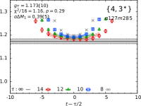
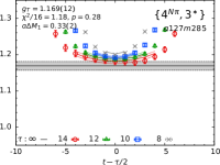
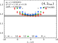
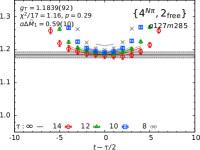
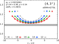
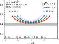
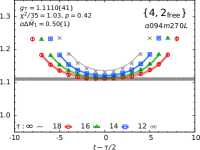
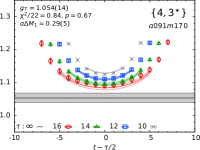
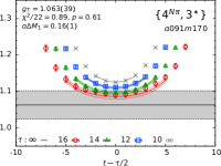
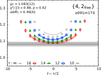
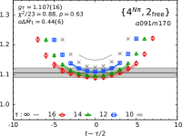
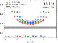
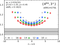
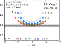
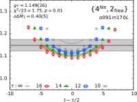
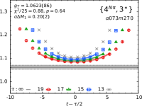
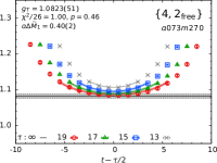
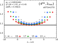
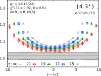
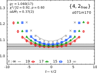
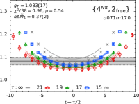
Figure 19: Each panel shows the data for the ratio defined in Eq. (19) that gives the unrenormalized tensor charge $g_{T}^{u-d}$ in the limit $\tau\to\infty$, and plotted as a function of $t-\tau/2$ for the four largest values of $\tau$. The rest is the same as in Fig. 17.

• The $\chi^{2}/$dof of fits with all four strategies are, again, reasonable and consistent as shown in Fig. 19.

• The $\Delta{\widetilde{M}}_{1}$ from $\{4,2^{\rm free}\}$ and $\{4^{N\pi},2^{\rm free}\}$ strategies is determined with similar precision (5–15% error) as from the $\{4^{N\pi}\}$ and $\{4\}$ fits to the two-point function. It is, however, much larger and comparable to the values found in the $g_{S}$ analysis as shown in Table 2. Thus, the same argument made in the case of $g_{S}$ for choosing results from $\{4,3^{\ast}\}$ or $\{4^{N\pi},3^{\ast}\}$ applies.

• The $\{4,2^{\rm free}\}$ and $\{4^{N\pi},2^{\rm free}\}$ estimates are systematically larger by 1–2$\sigma$ as can be seen in Fig. 19 and from Table 5. This is because a larger $\Delta{\widetilde{M}}_{1}$ leads to a smaller $\tau\to\infty$ extrapolation and thus a larger $g_{T}$ because convergence is from above.

• We note a roughly $1\sigma$ difference between $\{4,3^{\ast}\}$ and $\{4^{N\pi},3^{\ast}\}$ results on the $a091m170L$ and $a071m170$ ensembles, as shown in Fig. 3. While this $\approx 2\%$ difference is well within our error estimates, future calculations, especially at $M_{\pi}\approx 135$ MeV, are needed to confirm whether the low-lying multihadron states make a contribution at the few percent level as $M_{\pi}\to 135$ MeV.

• For the $\{4^{N\pi},2^{\rm free}\}$ strategy, the gray band in Fig. 19 showing the $\tau=\infty$ value lies above the largest $\tau$ data. This happens because the ratio data need not converge monotonically for specific combinations of $\Delta{\widetilde{M}}_{1}$ (or $\Delta{M}_{1}^{4^{\rm N\pi}}$) and the size of the ESC in the three-point function. An example is when the contribution of the excited states in the three-point function comes with a positive sign (as for $g_{T}$ that converges from above) while that from the two-point correlator always comes with a negative sign. (The spectral decomposition of the two-point function in the denominator is a sum of positive terms because our source and sink interpolating operators are the same.) We have checked that this behavior describes our data, and leads to a nonmonotonic convergence in the ratio for $g_{T}$, i.e., the ratio data go below the gray band as $\tau$ is increased and then turn back up at values of $\tau$ larger than accessible in current calculations. Our fits to the three-point correlators, which show monotonic convergence in $\tau$, are, on the other hand, robust.

Overall, as for $g_{S}$, the $\chi^{2}$/dof of the various fits to the data do not help us select among the strategies. We, therefore, perform the CCFV extrapolation for all four strategies in Sec. XIII.1 and then discuss our choice of the best estimate.

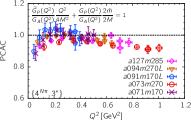
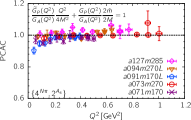
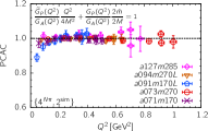
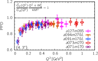
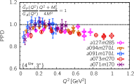
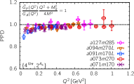
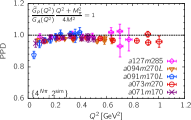
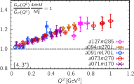
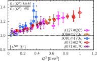
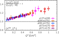
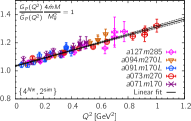
Figure 4: The top four panels show tests of the PCAC relation between the axial form factors for four analysis strategies specified at the bottom left corner. The middle panels show tests of the pion-pole dominance (PPD) hypothesis and the bottom panels show the quantity $4M_{N}{\widehat{m}}G_{P}(Q^{2})/M_{\pi}^{2}{\widetilde{G}}_{P}(Q^{2})$ that should equal unity for the PPD and the PCAC relation to be simultaneously satisfied. A fit linear in $Q^{2}$ is shown in the bottom right panel. The symbols and color code used to show the data from the five larger volume ensembles are specified in the legends. Only data with $Q^{2}\leq 1$ GeV² are shown as the errors above it are large in some cases.

IX The $A_{4}$ three-point function at $Q^{2}\neq 0$ and Understanding ESC in $G_{A}(Q^{2})$

In Ref. Jang et al. (2020a), we showed that the first excited state energies $M_{1}$ and $E_{1}$, obtained from the four-state fit $\{4\}$, are much larger than those of the noninteracting multihadron states relevant for extracting axial form factors: $N({\bm{q}})\pi({-\bm{q}})$ or $N({\bm{0}})\pi({-\bm{q}})$, or $N\pi\pi$ or even the $N(1440)$. The differences are striking at small momentum transfers. In fact, as illustrated in Fig. 1, estimates of $E_{1}$ have large uncertainty, and only the ground state parameters are determined with few percent accuracy from fits to the two-point functions. Even for $M_{0}$, in spite of the seemingly long plateau in the effective-mass plots starting at $\tau\sim 1$ fm, estimates from $\{4\}$- and $\{4^{N\pi}\}$-state fits differ by 1–2%. In Ref. Jang et al. (2020a), we also showed that when ${\widetilde{E}}_{1}$ extracted from two-state fits to the $A_{4}$ three-point function $\langle{\cal N}(\tau,-\bm{q})A_{4}(t,\bm{q})\overline{\cal N}(0,\bm{0})\rangle$ is used to obtain $G_{A}$, $\widetilde{G}_{P}$ and $G_{P}$, the PCAC relation between the three form factors is much better satisfied. That strategy, labeled $S_{\rm A4}$ in Jang et al. (2020a), is called $\{4,2^{\rm A_{4}}\}$ or $\{4^{N\pi},2^{\rm A_{4}}\}$ in this paper.

With high statistics data, we further explore the two- and three-state fits to the $A_{4}$ correlator at nonzero momentum transfer. We can now make fits with the full covariance matrix and can take the first excited state parameters from two-point correlators or leave $M_{1}$ and $E_{1}$ free along with the matrix elements, i.e., take only $M_{0}$, $E_{0}$, ${\cal A}_{0}$ and ${\cal A}_{0}^{\bm{p}}$ from one of the two four-state fits to the two-point function. To quantify the sensitivity of the form factors to different choices for the mass gaps, we investigate six strategies: $\{4,3^{\ast}\}$, $\{4^{N\pi},3^{\ast}\}$, $\{4,2^{\rm A_{4}}\}$, $\{4^{N\pi},2^{\rm A_{4}}\}$, $\{4,2^{\rm sim}\}$ and $\{4^{N\pi},2^{\rm sim}\}$. The last two involve a simultaneous fit, with common ${\widetilde{M}}_{1}$ and ${\widetilde{E}}_{1}$, to all four $A_{\mu}$ and the $P$ three-point functions as discussed below. A more detailed discussion of the possible excited states and the limitations of analyses is given in Appendix E.

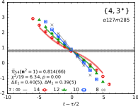
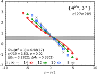
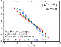
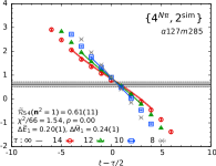
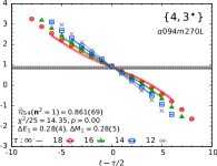
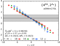
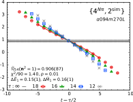
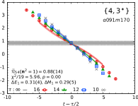
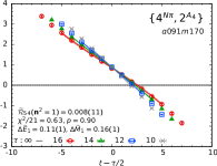
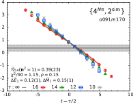
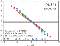
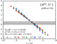
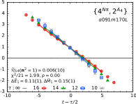
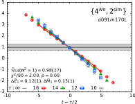
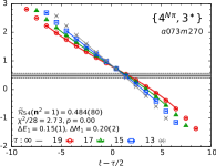
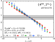
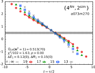
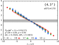
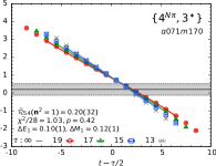
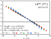
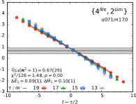
Figure 23: The ratio $R_{54}$, defined in Eq. (23), is plotted versus the shifted operator insertion time $t-\tau/2$ for ${\bm{n}}=(0,0,1)$. Results of the fits with $\{4,3^{\ast}\}$ (left column), $\{4^{N\pi},3^{\ast}\}$ ( second column), $\{4^{N\pi},2^{A_{4}}\}$ (third), and $\{4^{N\pi},2^{\rm sim}\}$ (right) strategies are shown by lines connecting the data points. The $\tau\to\infty$ value is shown by the gray band. The $y$-axis interval is the same for a given row to facilitate comparison of the result and the error. The legends give the analysis strategy, the ensemble ID, the ground state value (the gray band), the $\chi^{2}/$dof and the $p$-value of the fit, and the mass gaps, $\Delta M_{1}$ and $\Delta E_{1}$ (or $\Delta{\widetilde{M}}_{1}$ and $\Delta{\widetilde{E}}_{1}$ for $\{2^{A_{4}}\}$ or $\{2^{\rm sim}\}$ fits), of the first excited state on the two sides of the operator. For each $\tau$, only the data points connected by lines with the same color as the symbols are included in the simultaneous fits.

The first comparison of such fits to the three-point function $\langle{\cal N}(\tau)A_{4}(t)\overline{\cal N}(0)\rangle$ is shown in Fig. 23 for the four strategies $\{4,3^{\ast}\}$, $\{4^{N\pi},3^{\ast}\}$, $\{4^{N\pi},2^{\rm A_{4}}\}$ and $\{4^{N\pi},2^{\rm sim}\}$. Data from six ensembles are shown for momentum transfer ${\bm{n}}=(0,0,1)$ as these have large ESC. For the $\{4,3^{\ast}\}$ strategy, the $\chi^{2}/$dof of the fits, given in the labels in Fig. 23, are uniformly bad as was pointed out in Ref. Jang et al. (2020a). Also, as shown in Fig. 4, the form factors obtained with this strategy do not satisfy the PCAC relation rewritten as

$$\frac{Q^{2}}{4M_{N}^{2}}\frac{{\widetilde{G}}_{P}(Q^{2})}{G_{A}(Q^{2})}+\frac{2{\widehat{m}}}{2M_{N}}\frac{G_{P}(Q^{2})}{G_{A}(Q^{2})}=1\,,$$ (29)

with $\widehat{m}$ given in Table 1. Even though $\{4,3^{\ast}\}$ data fail the PCAC test, we will continue to perform a full analyses with it for the purpose of comparison.

The $\chi^{2}/$dof improves significantly with $\{4^{N\pi},3^{\ast}\}$ and is the best with $\{4^{N\pi},2^{\rm A_{4}}\}$ as shown in Fig. 23. The $\chi^{2}/$dof of the $\{4^{N\pi},2^{\rm sim}\}$ fit is similar, however, recall it involves a simultaneous fit to all five correlators. Also, estimates of ${\widetilde{M}}_{1}$ and ${\widetilde{E}}_{1}$ are similar in the two cases. The same is true with respect to satisfying PCAC as shown in Fig. 4.

Next, note that $\Delta M_{1}$ and $\Delta E_{1}$ decrease on going from $\{4,3^{\ast}\}$ to $\{4^{N\pi},3^{\ast}\}$ to $\{4^{N\pi},2^{\rm A_{4}}\}$; and the difference between $\Delta M_{1}$ and $\Delta E_{1}$ also changes. Overall, the behavior using strategy $\{4^{N\pi},2^{\rm A_{4}}\}$ is consistent with the results in Ref. Jang et al. (2020a), i.e., (i) the $\chi^{2}/{\rm dof}$ of the fits are much reduced; (ii) the ${\widetilde{M}}_{1}$ and ${\widetilde{E}}_{1}$, which we label as ${\widetilde{M}}_{1}^{A_{4}}$ and ${\widetilde{E}}_{1}^{A_{4}}$, are much smaller than those obtained from the $\{4\}$-fits to the two-point correlation function; and (iii) ${\widetilde{M}}_{1}^{A_{4}}$ and ${\widetilde{E}}_{1}^{A_{4}}$ are roughly consistent with the noninteracting energies of $N({\bm{q}})\pi({-\bm{q}})$ and $N({\bm{0}})\pi({-\bm{q}})$ states, respectively, as shown in Fig. 22. These features are also consistent with the effective field theory ($\chi$PT) result that, at leading (tree) order, the axial current inserts a pion with momentum $\bm{q}$, i.e., the pion-pole dominance (PPD) hypothesis Bär, Oliver (2019a, b).

In contrast, fits to the $A_{i}$ correlators with ${\widetilde{M}}_{1}$ and ${\widetilde{E}}_{1}$ left as free parameters do not have good $\chi^{2}/{\rm dof}$, i.e., these correlators do not constrain the excited-state parameters. The reason is that the ground state dominates in the $A_{i}$ correlators, whereas the excited state is dominant in $A_{4}$.

Using the ${\widetilde{M}}_{1}$ and ${\widetilde{E}}_{1}$ obtained from fits to $A_{4}$ to also analyze $A_{i}$ and $P$ leads to form factors that are in much better agreement with PCAC relation as shown in Fig. 4. This step, however, assumes that the same combination of excited states provides the dominant contribution to all five ($O=A_{\mu}$ and $P$) correlation functions. If this is the case then, statistically, the more sound method is to fit these five correlators simultaneously with common ${\widetilde{M}}_{1}$ and ${\widetilde{E}}_{1}$. These strategies are labeled $\{4,2^{\rm sim}\}$ and $\{4^{N\pi},2^{\rm sim}\}$. As expected, the resulting ${\widetilde{M}}_{1}$ and ${\widetilde{E}}_{1}$ from these simultaneous fits are similar to $M_{1}^{A_{4}}$ and $E_{1}^{A_{4}}$ because these are mainly controlled by the $A_{4}$ correlator.

Figure 4 also shows tests of the pion-pole dominance hypothesis, which, with the Goldberger-Treiman relation Goldberger and Treiman (1958), relates ${\widetilde{G}}_{P}(Q^{2})$ to $G_{A}(Q^{2})$ as

$$\frac{Q^{2}+M_{\pi}^{2}}{4M_{N}^{2}}\frac{{\widetilde{G}}_{P}(Q^{2})}{G_{A}(Q^{2})}=1\,.\\$$ (30)

The behavior of the data for the combination in Eq. (29) (PCAC) and Eq. (31) (PPD) is very similar and correlated, and $\{4^{N\pi},2^{\rm sim}\}$ gives the most consistent outcome. Noting this strong correlation, we examine the relation

$$2{\widehat{m}}\frac{2M_{N}}{M_{\pi}^{2}}\frac{G_{P}(Q^{2})}{{\widetilde{G}}_{P}(Q^{2})}=1\,,$$ (31)

which should hold for the PCAC relation, Eq. (29), and PPD, Eq. (30), to be simultaneously satisfied. Following Ref. Bernard, Veronique and Elouadrhiri, Latifa and Meißner, Ulf-G. (2002), and working to first order in $\chi$PT in $M_{\pi}^{2}$ and $Q^{2}$, the left hand side of Eq. (31) can be expanded as

$$1+\Delta+\frac{1}{6}\langle r^{2}_{A}\rangle M^{2}_{\pi}+\frac{Q^{2}}{M^{2}_{\pi}}\left(\Delta+\frac{1}{6}\langle r^{2}_{A}\rangle M^{2}_{\pi}\right)\,,$$ (32)

where $\Delta\equiv 2{\overline{d}}_{18}M_{\pi}^{2}/g_{A}$ is the Goldberger-Treiman discrepancy, and ${\overline{d}}_{18}$ is an unknown low-energy constant. The data for the left hand side of Eq. (31), also presented in Fig. 4, show that the ratio is close to unity at $Q^{2}=0$ and has a significant, essentially linear, increase with $Q^{2}$ on all seven ensembles. A linear fit to the five larger volume ensembles, shown in the bottom right panel in Fig. 4, gives $1.033(5)+0.272(16)Q^{2}$, with $Q^{2}$ in GeV². From Eq. (32), the quantity $(\Delta+\frac{1}{6}\langle r^{2}_{A}\rangle M^{2}_{\pi})$ should equal the intercept minus one, and also the slope times $M_{\pi}^{2}$. Using our result $\langle r^{2}_{A}\rangle=0.43$ fm² presented in Sec. XIII.2, we get $\Delta\sim 0$ from the intercept and $\sim-0.02$ from the slope. For comparison, using the Goldberger-Treiman relation $g_{A}M_{N}=g_{\pi NN}F_{\pi}(1+\Delta)$ and the experimental values $g_{A}=1.27641$, $M_{N}=939$ MeV, $F_{\pi}=92.2$ MeV and $g_{\pi NN}=13.25$ Navarro Pérez et al. (2017); Reinert et al. (2021); Baru et al. (2011) gives $\Delta\sim-0.02$. In short, we show that the ratio defined in Eq. (31) is not unity, and exhibits a linear dependence on $Q^{2}$ that is consistent with the prediction of $\chi$PT.

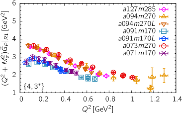
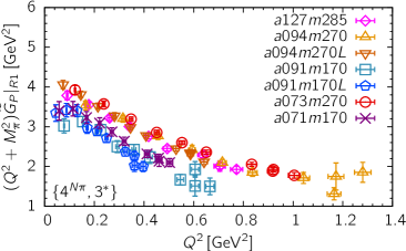
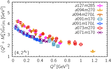
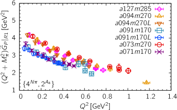
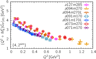
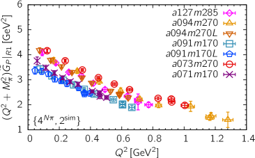
Figure 26: The data for $(Q^{2}+M_{N}^{2}){\widetilde{G}}_{P}(Q^{2})$ from the seven ensembles are plotted versus $Q^{2}$. According to the pion-pole dominance hypothesis, Eq. (30), the result should be a smooth monotonic function that is proportional to $G_{A}(Q^{2})$. The data from the $\{4,3^{\ast}\}$ and $\{4^{N\pi},3^{\ast}\}$ strategies on the $M_{\pi}=170$ MeV ensembles (top two panels) show deviations from this expectation at small $Q^{2}$. Also, the “lines” of data from a given ensemble move up slightly as $a\to 0$ and down as $M_{\pi}\to 135$ MeV. The labels specify the analysis strategy and the ensemble ID.

The data in Fig. 4 also show that with the $\{4^{N\pi},2^{\rm sim}\}$ strategy, the smallest $Q^{2}$ points on the $a091m170L$ ensemble start to deviate away from unity for both the PCAC and PPD relations but not those from the $a071m170$ ensemble. In contrast, for the $\{4,3^{\ast}\}$ strategy, the data from both ensembles bend down at small $Q^{2}$, which we have shown is due to the missed $N\pi$ states. To investigate this difference between the $a091m170L$ and $a071m170$ data with the $\{4^{N\pi},2^{\rm sim}\}$ strategy, we show $(Q^{2}+M_{\pi}^{2}){\widetilde{G}}_{P}(Q^{2})$ versus $Q^{2}$ in Fig. 26 in Appendix F, and note that the data move up as $a\to 0$ for all but the $\{4,3^{\ast}\}$ strategy, i.e., they indicate a dependence on $a$ when the $N\pi$ state is included. Nevertheless, we cannot pinpoint whether the difference in behavior is a discretization effect or a combination of statistical and/or larger discretization effects in the $a091m170L$ data, or indicates the need to include additional [multihadron] low energy excited states in the fits. In the near future, we plan to double the statistics on these two ensembles to better quantify the difference and explore adding a third state, i.e., a $\{4^{N\pi},3^{\rm sim}\}$ fit.

IX.1 $\{4^{N\pi},2^{\rm sim}\}$ is our preferred strategy for analyzing the axial form factors

Data from the two strategies $\{4^{N\pi},2^{A_{4}}\}$ and $\{4^{N\pi},2^{\rm sim}\}$ show much better agreement with the PCAC and PPD relations as shown in Fig. 4. To choose between them, we consider two additional checks: First, the ground state matrix elements extracted from the $A_{4}$ correlator with ${\bm{q}}\neq 0$ should satisfy the relation $\partial_{4}A_{4}=(E_{0}-M_{0})A_{4}$ for all $\bm{q}$. Second, the value of the ground state matrix element $\langle{N}|A_{4}|N\rangle$ extracted from fits to $\langle{\cal N}A_{4}{\cal N}\rangle$ should agree with that reconstructed by inserting $G_{A}$ and $\widetilde{G}_{P}$ calculated from the $A_{i}$ correlators into the right hand side of Eq. (23). The first condition is satisfied by both strategies even though $\langle{N}|A_{4}|N\rangle$ is very poorly determined with $\{4^{N\pi},2^{A_{4}}\}$. The second check is satisfied within errors only by data from $\{4^{N\pi},2^{\rm sim}\}$. Based on these two consistency checks and the PCAC relation, we select $\{4^{N\pi},2^{\rm sim}\}$ as our preferred strategy for analyzing the axial form factors, however, we will continue to examine all six strategies discussed above to exhibit the spread.

The obvious next step is $\{4^{N\pi},3^{\rm sim}\}$ fits, i.e., leaving the first and second excited-state energy gaps as free parameters (or using priors for them) in fits to the three-point functions. With current data, we do not get meaningful results. Much higher statistics are required.

X Axial vector form factors

As discussed in Sec. IX, we compare six strategies to extract the axial vector form factors, with our preferred one being $\{4^{N\pi},2^{\rm sim}\}$. It makes the following assumption: the excited-state contamination in all five channels, $A_{\mu}$ and $P$, can, to a good approximation, be accounted for by a “single low mass effective excited state” whose parameters can be determined from a simultaneous two-state fit to the five three-point functions. Only the ground state parameters are taken from fits to the two-point functions.

We find that the two sets of estimates using $\{4^{N\pi},2^{A_{4}}\}$ and $\{4^{N\pi},2^{\rm sim}\}$, versus $\{4,2^{A_{4}}\}$ and $\{4,2^{\rm sim}\}$ fits give overlapping results for the form factors, which satisfy PCAC equally well. These two sets differ only in the $M_{0}$ and ${\cal A}_{0}$ obtained from the $\{4^{N\pi}\}$- and $\{4\}$-state fits to the two-point functions, and these differences do not significantly impact the results for the form factors. It is the mass gap of the first excited state used in the fits to the three-point function that is important. In both the $\{2^{A_{4}}\}$ and $\{2^{\rm sim}\}$ fits, the output $\Delta{\widetilde{E}}_{1}$ is controlled by the $A_{4}$ correlator and corresponds to the $N\pi$ state as discussed in Sec. IX. Thus, the impact of including the $N\pi$ state is far more significant in the 3-point functions, however, our approach is to consistently choose strategies in which the mass gap in both the two- and three-point functions does or does not include the low-lying ($N\pi$) state. This is achieved with the $\{4,3^{\ast}\}$, $\{4^{N\pi},3^{\ast}\}$, $\{4^{N\pi},2^{A_{4}}\}$ and $\{4^{N\pi},2^{\rm sim}\}$ strategies (see Appendix A for their definition), which are, therefore, used to present the final results. We do not discuss estimates from the $\{4,2^{A_{4}}\}$ and $\{4,2^{\rm sim}\}$ strategies any further since all we can add from their analysis is they give results consistent with $\{4^{N\pi},2^{A_{4}}\}$ and $\{4^{N\pi},2^{\rm sim}\}$.

The data for $Z_{A}{G}_{A}(Q^{2})$ and $Z_{A}{\widetilde{G}}_{P}(Q^{2})$ for the four remaining strategies are given in Tables 18 and 19 and plotted in Figs. 5 and 6, where we divide them by $g_{A}^{\rm exp}=1.277$ so that the value should equal unity at $Q^{2}=0$ in the CCFV limit. Similarly, the unrenormalized ${G}_{P}(Q^{2})$ is given in Table 20 and plotted in Fig. 7. The latter is used primarily to check the PCAC and PPD relations as shown in Fig. 4.

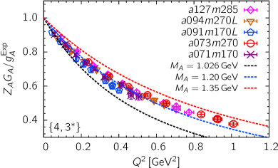
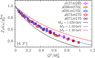
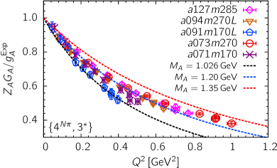
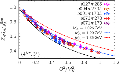
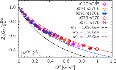
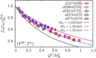
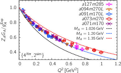
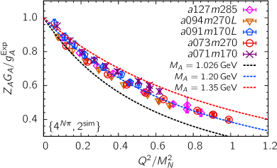
Figure 5: The data for the renormalized axial form factor $Z_{A}G_{A}(Q^{2})/g_{A}^{\rm exp}$, with $g_{A}^{\rm exp}=1.277$, are plotted versus $Q^{2}$ in GeV² (left) and $Q^{2}/M_{N}^{2}$ (right). Each panel shows the data from the five larger volume ensembles. The four rows show the results from four strategies, specified at the lower left corner of each panel that are used to control ESC. The three curves show the dipole ansatz with $M_{A}=1.026$, 1.2 and 1.35 GeV, and have been drawn only to guide the eye. The agreement of the three $\sim 270$ and the two 170 MeV data indicates that discretization errors are small.

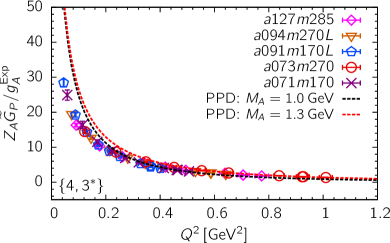
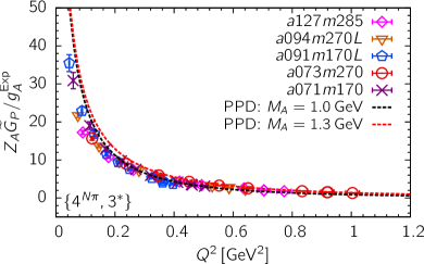
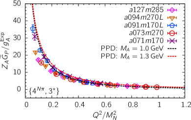
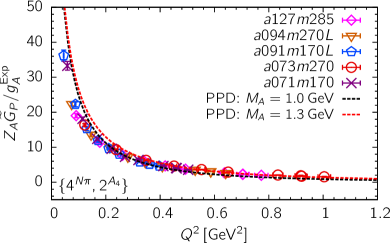
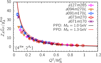
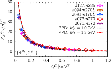
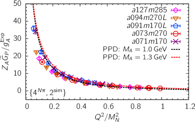
Figure 6: The data for the renormalized induced pseudoscalar form factor $Z_{A}{\widetilde{G}}_{P}(Q^{2})/g_{A}^{\rm exp}$, with $g_{A}^{\rm exp}=1.277$, are plotted versus $Q^{2}$ in GeV² (left) and $Q^{2}/M_{N}^{2}$ (right). Each panel shows the data from the five larger volume ensembles. The four rows show the results from four strategies for controlling ESC that are specified in the label at the bottom left corner. The difference among the three $\sim 270$ and the two 170 MeV data is more noticeable when plotted versus $Q^{2}/M_{N}^{2}$.

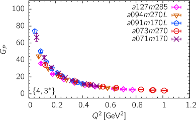
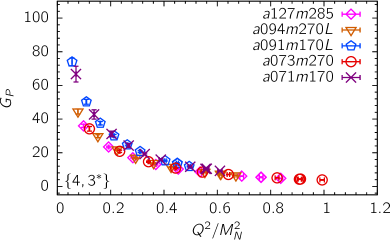
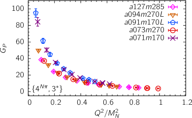
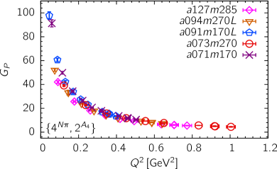
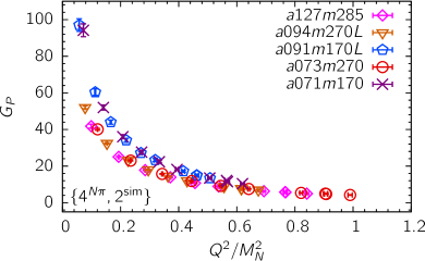
Figure 7: The unrenormalized pseudoscalar form factor ${G}_{P}(Q^{2})$ is plotted versus $Q^{2}$ in GeV² (left) and $Q^{2}/M_{N}^{2}$ (right). Each panel shows the data from the five larger volume ensembles. The four rows show the results from four strategies for controlling ESC that are specified in the labels. The difference among the three $\sim 270$ MeV and the two 170 MeV data is more noticeable when plotted versus $Q^{2}/M_{N}^{2}$.

fit	$\langle r_{A}^{2}\rangle|_{\text{dipole}}$	$\langle r_{A}^{2}\rangle|_{P_{2}}$	$\langle r_{A}^{2}\rangle|_{z^{2}}$
$a127m285$
$\{4,3^{\ast}\}$	0.293(13)	0.293(20)	0.297(15)
$\{4^{N\pi},3^{\ast}\}$	0.315(13)	0.333(22)	0.323(15)
$\{4^{N\pi},2^{A_{4}}\}$	0.302(15)	0.349(32)	0.315(18)
$\{4^{N\pi},2^{\text{sim}}\}$	0.304(15)	0.310(42)	0.297(21)
$a094m270$
$\{4,3^{\ast}\}$	0.255(18)	0.293(65)	0.291(29)
$\{4^{N\pi},3^{\ast}\}$	0.265(14)	0.340(43)	0.314(18)
$\{4^{N\pi},2^{A_{4}}\}$
$\{4^{N\pi},2^{\text{sim}}\}$	0.247(11)	0.280(48)	0.278(23)
$a094m270L$
$\{4,3^{\ast}\}$	0.290(11)	0.305(18)	0.305(13)
$\{4^{N\pi},3^{\ast}\}$	0.317(11)	0.348(20)	0.336(13)
$\{4^{N\pi},2^{A_{4}}\}$	0.312(9)	0.358(19)	0.339(12)
$\{4^{N\pi},2^{\text{sim}}\}$	0.298(10)	0.333(26)	0.317(16)
$a091m170$
$\{4,3^{\ast}\}$	0.301(15)	0.307(30)	0.340(29)
$\{4^{N\pi},3^{\ast}\}$	0.376(33)	0.355(92)	0.411(69)
$\{4^{N\pi},2^{A_{4}}\}$	0.292(16)	0.459(52)	0.466(41)
$\{4^{N\pi},2^{\text{sim}}\}$	0.306(16)	0.350(59)	0.378(53)
$a091m170L$
$\{4,3^{\ast}\}$	0.341(19)	0.323(30)	0.342(30)
$\{4^{N\pi},3^{\ast}\}$	0.449(45)	0.426(74)	0.462(63)
$\{4^{N\pi},2^{A_{4}}\}$	0.311(20)	0.486(48)	0.484(40)
$\{4^{N\pi},2^{\text{sim}}\}$	0.369(19)	0.478(61)	0.479(51)
$a073m270$
$\{4,3^{\ast}\}$	0.269(12)	0.270(24)	0.280(17)
$\{4^{N\pi},3^{\ast}\}$	0.271(9)	0.330(22)	0.312(12)
$\{4^{N\pi},2^{A_{4}}\}$	0.242(9)	0.287(21)	0.271(14)
$\{4^{N\pi},2^{\text{sim}}\}$	0.253(8)	0.285(22)	0.278(13)
$a071m170$
$\{4,3^{\ast}\}$	0.284(22)	0.288(36)	0.306(38)
$\{4^{N\pi},3^{\ast}\}$	0.368(29)	0.428(66)	0.455(56)
$\{4^{N\pi},2^{A_{4}}\}$	0.271(15)	0.494(47)	0.507(39)
$\{4^{N\pi},2^{\text{sim}}\}$	0.308(18)	0.424(67)	0.438(59)

Table 6: Results for $\langle r_{A}^{2}\rangle$ from a dipole, $P_{2}$ Padé and $z^{2}$ fits to all ten $Q^{2}\neq 0$ points for the seven ensembles and the four strategies in column 1 (see Appendix A), used to control excited state contamination. The fits to $\{4^{N\pi},2^{A_{4}}\}$ data on the $a094m270$ ensemble are not stable so no results are given.

X.1 Parameterizing the $Q^{2}$ behavior of $G_{A}(Q^{2})$ and the extraction of $g_{A}$ and $\langle r_{A}^{2}\rangle$

Our primary goal is to calculate the axial form factors, $G_{A}$ and ${\widetilde{G}}_{P}$, as a function of $Q^{2}$ as these are needed in the calculation of the neutrino-nucleus cross-sections. These results are shown in Figs. 5 and 6.

In most current lattice QCD calculations, the smallest nonzero lattice momentum, which is also the gap between the discrete momenta, is large, $|\bm{q}_{\rm min}|\geq 200$ MeV. Consequently, it is important to keep in mind that obtaining the slope and the value at $Q^{2}=0$ from fits to lattice data with $Q^{2}\gtrsim 0.04$ GeV² have an associated systematic uncertainty. This can be estimated by comparing $g_{A}$ obtained directly at $Q^{2}=0$ from the forward matrix element with the extrapolated value $G_{A}(Q^{2}\to 0)$. In this work, we perform this extrapolation using three parameterizations, dipole, Padé and $z$-expansion, as discussed below and in Sec. XIII.1.

Historically, the dipole ($D$) ansatz has been used to parameterize the $Q^{2}$ behavior of $G_{A}(Q^{2})$:

$$G_{A}(Q^{2})|_{D}=\frac{G_{A}(0)}{(1+Q^{2}/{\cal M}_{A}^{2})^{2}}\ \Longrightarrow\ \langle r_{A}^{2}\rangle=\frac{12}{{\cal M}_{A}^{2}}\,.$$ (33)

It is the Fourier transform of a distribution exponentially falling in space, and appealing for phenomenological analyses because it has only one unknown parameter, the axial mass ${\cal M}_{A}$ since $g_{A}$ is known accurately from experiments. Also, it goes to zero as $Q^{4}$ for large $Q^{2}$ as predicted by QCD perturbation theory Smith and Moniz (1972); Lepage and Brodsky (1980).

The second parameterization used is the model-independent $z$-expansion Hill and Paz (2010); Bhattacharya et al. (2011):

$$\frac{G_{A}(Q^{2})}{G_{A}(0)}=\sum_{k=0}^{\infty}a_{k}z(Q^{2})^{k}\,,$$ (34)

where the $a_{k}$ are fit parameters and $z$ is defined to be

$$z=\frac{\sqrt{t_{\text{cut}}+Q^{2}}-\sqrt{t_{\text{cut}}+{\overline{t}}_{0}}}{\sqrt{t_{\text{cut}}+Q^{2}}+\sqrt{t_{\text{cut}}+{\overline{t}}_{0}}}\,.$$ (35)

In terms of $z$, the form factors are analytical within the unit circle with the nearest singularity, a branch cut, at $Q^{2}=-t_{\text{cut}}=-9M_{\pi}^{2}$ (or $-4M_{\pi}^{2}$ in the vector channel). We choose the parameter ${\overline{t}}_{0}$, which is the value of $-Q^{2}$ that is mapped to $z=0$, to be the midpoint of the range of $Q^{2}$ values on each ensemble to minimize the maximum value of $|z|$ as discussed in Ref. Jang et al. (2020a). For the seven ensembles listed in Table 15, this corresponds to ${\overline{t}}_{0}=\{0.4,\ 0.6,\ 0.3,\ 0.3,\ 0.2,\ 0.5,\ 0.25\}$ GeV², respectively. We find no significant difference in the results on using ${\overline{t}}_{0}=0$.

The data for $Z_{A}G_{A}(Q^{2})/1.277$ are plotted versus $z$ in Fig. 8 for the $\{4^{N\pi},2^{\rm sim}\}$ strategy and show only small deviations from linearity. As a result, $z$-expansion fits with $z^{\{2,3,4\}}$ truncations give essentially identical results for both $g_{A}$ and $\langle r_{A}^{2}\rangle$. As shown in Fig. 9, the augmented $\chi^{2}$ does not decrease by two units on increasing the order of truncation from $z^{2}\to z^{3}\to z^{4}$. Therefore the $z^{\{3,4\}}$ fits are considered overparameterized by the Akaike information criteria Akaike (1974). In Ref. Jang et al. (2020b), we had observed that fitting the precise experimental data for the electric and magnetic form factors stabilizes for $z^{k}$ truncated at $k\geq 4$. Our current lattice data with ten points are well fit by the $z^{2}$ ($z^{3}$) truncation for the axial (vector) form factors as discussed further in Sec. XII.

Figure 8: The renormalized $G_{A}$ plotted versus $z$ for the seven ensembles. The data are from the $\{4^{N\pi},2^{\rm sim}\}$ strategy.

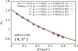
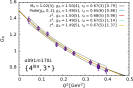
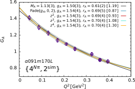
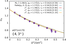
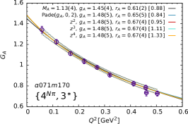
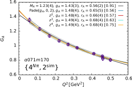
Figure 9: Plot of $G_{A}$ versus $Q^{2}$ for the $a091m170L$ (top row) and $a071m170$ (bottom row) ensembles. Also shown are the dipole, Padé ($g_{A}$,0,2) and $z^{\{2,3,4\}}$ fits to the ten $Q^{2}$ points. The results for unrenormalized $g_{A}$ and $r_{A}$ (in fm) are given in the legends: dipole (top line), Padé (second line) and $z^{2,3,4}$ (lines 3-5). The $\chi^{2}$/dof of the fits are given within square brackets. The error bands of the fits are shown by dotted lines of the same color only over the range of the data for clarity.

ESC strategy	$c_{0}$	$c_{1}$	$c_{2}$	$c_{3}$	[$\chi^{2}/dof$]	$g_{P}^{\ast}|_{{\rm Z}_{1}}$	$g_{\pi NN}|_{{\rm Z}_{1}}$	$g_{P}^{\ast}|_{{\rm Z}_{2}}$	$g_{\pi NN}|_{{\rm Z}_{2}}$
$Q^{2}$ fits to the $a091m170L$ data
$\{4,3^{\ast}\}$	0.0356(16)	0.136(37)	-2.13(30)	-	[29.38/7]	3.89(15)	7.52(39)	3.87(15)	7.50(38)
$\{4,3^{\ast}\}$	0.0312(18)	0.545(93)	-11.8(2.0)	65(13)	[6.22/6]	3.76(16)	6.59(42)	3.75(15)	6.57(41)
$\{4^{N\pi},3^{\ast}\}$	0.0501(41)	-0.13(10)	-0.99(74)	-	[15.91/7]	5.19(36)	10.59(90)	5.17(36)	10.55(90)
$\{4^{N\pi},3^{\ast}\}$	0.0425(49)	0.43(23)	-14.0(4.7)	87(31)	[8.04/6]	4.86(38)	9.0(1.1)	4.84(38)	8.9(1.1)
$\{4^{N\pi},2^{A_{4}}\}$	0.0548(23)	-0.287(64)	0.86(48)	-	[3.59/7]	5.55(21)	11.56(57)	5.53(19)	11.53(54)
$\{4^{N\pi},2^{A_{4}}\}$	0.0530(33)	-0.18(15)	-1.2(2.9)	13(18)	[3.06/6]	5.45(25)	11.20(75)	5.43(23)	11.17(73)
$\{4^{N\pi},2^{\text{sim}}\}$	0.0529(25)	-0.196(83)	-0.05(71)	-	[4.02/7]	5.43(21)	11.17(60)	5.41(20)	11.13(58)
$\{4^{N\pi},2^{\text{sim}}\}$	0.0516(40)	-0.11(21)	-1.8(4.3)	12(28)	[3.85/6]	5.36(27)	10.90(89)	5.34(26)	10.86(88)
$Q^{2}$ fits to the $a071m170$ data
$\{4,3^{\ast}\}$	0.0192(17)	0.116(67)	-2.04(70)	-	[10.98/7]	3.69(27)	6.89(63)	3.71(27)	6.91(63)
$\{4,3^{\ast}\}$	0.0174(18)	0.47(14)	-13.7(4.1)	102(36)	[2.81/6]	3.66(27)	6.22(67)	3.67(27)	6.24(67)
$\{4^{N\pi},3^{\ast}\}$	0.0318(27)	-0.231(94)	0.32(92)	-	[7.43/7]	5.73(42)	11.38(99)	5.75(43)	11.4(1.0)
$\{4^{N\pi},3^{\ast}\}$	0.0271(34)	0.21(23)	-12.0(5.8)	104(48)	[2.82/6]	5.24(48)	9.7(1.3)	5.25(49)	9.7(1.3)
$\{4^{N\pi},2^{A_{4}}\}$	0.0325(11)	-0.295(49)	1.83(59)	-	[7.24/7]	5.81(17)	11.64(48)	5.83(17)	11.68(48)
$\{4^{N\pi},2^{A_{4}}\}$	0.0359(20)	-0.60(16)	10.0(4.2)	-67(34)	[3.34/6]	6.19(26)	12.87(80)	6.21(26)	12.91(80)
$\{4^{N\pi},2^{\text{sim}}\}$	0.0342(15)	-0.295(66)	1.22(76)	-	[2.54/7]	6.13(23)	12.24(61)	6.15(24)	12.28(62)
$\{4^{N\pi},2^{\text{sim}}\}$	0.0354(26)	-0.40(19)	4.1(5.0)	-24(41)	[2.20/6]	6.27(34)	12.69(98)	6.29(34)	12.73(98)

Table 7: Results of fits to $\frac{m_{\mu}}{2M_{N}}\widetilde{G}_{P}(Q^{2})$ versus $Q^{2}$ using the ansatz and the parameters $c_{i}$ defined in Eq. (38). The strategies used to remove ESC in column 1 are defined in Appendix A. Fits to $a091m170L$ data (top) and $a071m170$ (bottom), with and without the finite volume ($c_{3}$) term, are compared for the four strategies listed in column one. All ten values of $Q^{2}$ are used in the fits and results are given for both renormalization methods.

Ensemble	$\{4,3^{\ast}\}$		$\{4^{N\pi},2^{\rm sim}\}$		$\{4,3^{\ast}\}$		$\{4^{N\pi},2^{\rm sim}\}$
	$g_{P}^{\ast}|_{{\rm Z}_{1}}$	$g_{P}^{\ast}|_{{\rm Z}_{2}}$	$g_{P}^{\ast}|_{{\rm Z}_{1}}$	$g_{P}^{\ast}|_{{\rm Z}_{2}}$	$g_{\pi NN}|_{{\rm Z}_{1}}$	$g_{\pi NN}|_{{\rm Z}_{2}}$	$g_{\pi NN}|_{{\rm Z}_{1}}$	$g_{\pi NN}|_{{\rm Z}_{2}}$
$a127m285$	2.266(66)	2.221(61)	2.655(81)	2.602(78)	11.30(53)	11.08(51)	13.64(67)	13.37(65)
$a094m270$	2.52(16)	2.50(16)	2.87(10)	2.851(96)	11.27(89)	11.20(87)	12.97(59)	12.90(57)
$a094m270L$	2.455(94)	2.465(89)	2.919(68)	2.931(55)	10.89(56)	10.94(54)	13.46(46)	13.51(43)
$a091m170$	3.93(14)	3.91(14)	5.53(22)	5.50(21)	7.77(37)	7.73(36)	11.30(56)	11.24(55)
$a091m170L$	3.89(15)	3.87(15)	5.43(21)	5.41(20)	7.52(39)	7.50(38)	11.17(60)	11.13(58)
$a073m270$	2.45(11)	2.45(10)	2.883(54)	2.883(48)	11.11(62)	11.11(62)	13.30(40)	13.30(39)
$a071m170$	3.69(27)	3.71(27)	6.13(23)	6.15(24)	6.89(63)	6.91(63)	12.24(61)	12.28(62)

Table 8: Results for $g_{P}^{\ast}\equiv\frac{m_{\mu}}{2M_{N}}\widetilde{G}_{P}(0.88m_{\mu}^{2})$ and $g_{\pi NN}\equiv\frac{c_{0}}{2a^{2}m_{\mu}F_{\pi}}$ from fits to $\frac{m_{\mu}}{2M_{N}}\widetilde{G}_{P}(Q^{2})$ using Eq. (38) with the term proportional to $c_{3}$ set to zero. Estimates from the two renormalization methods and the two strategies $\{4,3^{\ast}\}$ and $\{4^{N\pi},2^{\rm sim}\}$ are compared.

We also examine $z$-expansion fits with sum rules that ensure that $G_{A}(Q^{2})$ falls as $Q^{-4}$ with $Q^{2}\to\infty$ as predicted by perturbation theory Lepage and Brodsky (1980) following the procedure described in Ref. Jang et al. (2020b). Results of analyses with and without sum rules overlap. Our final results for $g_{A}$ (Table 4) and $\langle r_{A}^{2}\rangle$ (Table 6) are taken from fits without sum rules as these quantities characterize the behavior at $Q^{2}=0$. To stabilize all these $z$-expansion fits, we use Gaussian priors for all the $a_{k}$ with central value zero and width five.

Last, we make two Padé fits, $P_{2}\equiv P(g,0,2)$ and $P_{3}\equiv P(g,1,3)$, defined as

$$P(g,0,2) =\frac{g}{1+b_{1}Q^{2}+b_{2}Q^{4}}\,,$$ (36)

$$P(g,1,3) =\frac{g(1+a_{1}Q^{2})}{1+b_{1}Q^{2}+b_{2}Q^{4}+b_{3}Q^{6}}\,.$$ (37)

These also incorporate the $1/Q^{4}$ behavior expected at large $Q^{2}$. Since the calculation is done for spacelike $Q^{2}$ and at values sufficiently far from the physical poles and cuts, their influence is expected to be small. Therefore, these Padé fits should provide an equally good parameterization as the $z$-expansion.

We find that $P_{2}$ gives results consistent with the $z^{2,3,4}$ fits, and has the virtue of being easier to visualize in terms of powers of $Q^{2}$. In Sec. XIV we will also present a $P(g,0,2)$ and $z^{2}$ (or $z^{3}$) parameterization of the axial, electric and magnetic form factors ignoring lattice artifacts, with results given in Eqs. (55), (56) and (58).

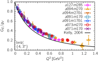
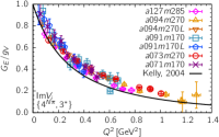
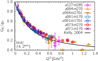
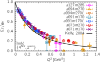
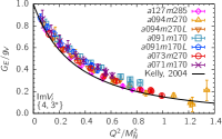
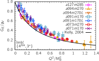
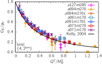
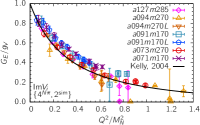
Figure 13: $G_{E}(Q^{2})$ from $\Im V_{i}$ plotted versus $Q^{2}$ in GeV² (top panels) and versus $Q^{2}/M_{N}^{2}$ (bottom panels). Each panel shows the data for the seven ensembles, and each row compares the four strategies used to remove ESC.

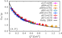
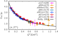
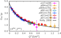
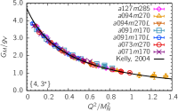
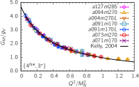
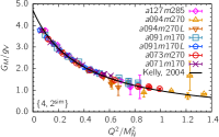
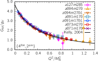
Figure 14: $G_{M}(Q^{2})$ from $\Re V_{i}$ plotted versus $Q^{2}$ in GeV² (top panels) and versus $Q^{2}/M_{N}^{2}$ (bottom panels). Each panel shows the data for the seven ensembles, and each row compares the four strategies used to remove ESC.

To explore systematic errors due to the limited range of $Q^{2}$ points fit, we compare results obtained by fitting all ten $Q^{2}\neq 0$ points versus the six with the smallest $Q^{2}$ values. This cut, based on the number of points rather than a value of $Q^{2}$ in physical units, is chosen because, in the problematic cases in the vector channel, the errors are large in the four largest $Q^{2}$ points as can be seen in Figs. 12–14. Based on this comparison, we selected ten-point fits for the axial form factors and six-point for the vector.

Results for $g_{A}$ and $\langle r_{A}^{2}\rangle$ depend on both the strategy used to obtain the ground state matrix element and on the fits (dipole, or the $z$-expansion or the Padé) used to parameterize the $Q^{2}$ behavior of $G_{A}(Q^{2})$. In particular, the value of the low $Q^{2}$ points in $G_{A}(Q^{2})$ vary between the strategies as shown in Fig. 21, which in turn leads to differences in the $Q^{2}$ parameterization, i.e., in $g_{A}$ and $\langle r_{A}^{2}\rangle$. These differences can be inferred from the labels in Fig. 9, where the three panels give $Q^{2}$ fits to $G_{A}(Q^{2}\neq 0)$ data for the $\{4,3^{\ast}\}$, $\{4^{N\pi},3^{\ast}\}$ and $\{4^{N\pi},2^{\rm sim}\}$ strategies for the $a091m170L$ and $a071m170$ ensembles. Recall that the difference in $g_{A}$, obtained from the forward matrix element, between the $\{4,3^{\ast}\}$ and $\{4^{N\pi},3^{\ast}\}$ strategies was shown in Fig. 3.

Comparing results for $g_{A}$ and $\langle r_{A}^{2}\rangle$ from the seven ensembles, summarized in Tables 4 and 6, we note the following points:

• With the $\{4,3^{\ast}\}$ strategy, results for $g_{A}$ from dipole, $z^{\{2,3,4\}}$ and Padé fits agree with those measured directly from the forward matrix element on all ensembles. The fits have reasonable $\chi^{2}$/dof.

• For the $\{4^{N\pi},3^{\ast}\}$ strategy, similar agreement is seen between results from the dipole, $z^{\{2,3,4\}}$ and Padé fits, and from the forward matrix element. However, these estimates are larger than those with the $\{4,3^{\ast}\}$ strategy, especially for the $M_{\pi}\approx 170$ MeV ensembles (see Fig. 3).

• With the $\{4^{N\pi},2^{A_{4}}\}$ and the preferred $\{4^{N\pi},2^{\rm sim}\}$ strategies, (i) the dipole estimates are smaller than the $z^{\{2,3,4\}}$ or the Padé values on all three $M_{\pi}=170$ MeV ensembles, and (ii) the $\chi^{2}$/dof becomes larger for the dipole fit to the data from all three $\{4^{N\pi}\}$ strategies, mainly because it misses the low $Q^{2}$ points.

A key point is that the differences observed on the $M_{\pi}\approx 170$ MeV ensembles are not evident at $M_{\pi}\sim 270$ MeV. This is consistent with the earlier discussion that the difference in the mass gaps between the $\{4\}$ and $\{4^{N\pi}\}$ fits become larger as $M_{\pi}$ decreases, i.e., the mass gap of the $N\pi$ state decreases. In short, the data shown in Tables 4 and 6 indicate that estimates of $g_{A}$ and $\langle r_{A}^{2}\rangle$ become increasingly sensitive to the ESC strategy as $M_{\pi}\to 135$ MeV. Also, the dipole fit starts to fail. This $M_{\pi}$ dependent behavior has a significant impact on the final estimates obtained from the CCFV fits as discussed in Sec. XIII and shown in Fig. 32.

XI The induced pseudoscalar form factor ${\widetilde{G}}_{P}(Q^{2})$ and the extraction of $g_{P}^{\ast}$ and $g_{\pi NN}$

The data for the renormalized induced pseudoscalar form factor $Z_{A}{\widetilde{G}}_{P}(Q^{2})/(g_{A}^{\rm exp})$ from the five larger volume ensembles are plotted versus $Q^{2}$ and $Q^{2}/M_{N}^{2}$ in Fig. 6. Overall, the data show dependence on the pion mass, i.e., data fall into two bands for ensembles with $M_{\pi}\approx 270$ and 170 MeV. This dependence is more evident when plotted versus $Q^{2}/M_{N}^{2}$. On the other hand, we do not observe a significant $a$ dependence.

The $Q^{2}$ dependence of ${\widetilde{G}}_{P}(Q^{2})$, given in Table 19, is analyzed using the small $Q^{2}$ expansion of the pion-pole dominance ansatz given in Eq. (30):

$$\frac{m_{\mu}}{2M_{N}}{\widetilde{G}}_{P}(Q^{2})=\frac{c_{0}}{a^{2}(M_{\pi}^{2}+Q^{2})}+c_{1}+c_{2}a^{2}Q^{2}+c_{3}a^{4}Q^{4}\,,$$ (38)

where the leading term is the pion-pole term and the polynomial approximates the dependence coming from the small $Q^{2}$ behavior of $G_{A}(Q^{2})$. It is also the behavior predicted for small $Q^{2}$ and $M_{\pi}^{2}$ by the leading order chiral perturbation theory Bernard, Veronique and Elouadrhiri, Latifa and Meißner, Ulf-G. (2002). In practice, this ansatz fits the data over a large range of $Q^{2}$, 2.5$M_{\pi}^{2}$ – 50$M_{\pi}^{2}$ in units of $M_{\pi}=135$ MeV, as given in Table 17.

From these fits, we extract $g_{P}^{\ast}$ and the pion-nucleon coupling, $\mathop{g_{\pi{NN}}}\nolimits$, using the following expressions:

$$g_{P}^{\ast}\equiv \;\frac{m_{\mu}}{2M_{N}}\widetilde{G}_{P}(0.88m_{\mu}^{2})\,,$$ (39)

$$g_{\pi NN}\equiv \;\lim_{Q^{2}\to-M_{\pi}^{2}}\frac{M_{\pi}^{2}+Q^{2}}{4M_{N}F_{\pi}}{\widetilde{G}}_{P}(Q^{2})=\frac{c_{0}}{2a^{2}m_{\mu}F_{\pi}}\,,$$ (40)

where $\mathop{g_{\pi{NN}}}\nolimits$ is defined as the residue of ${\widetilde{G}}_{P}(Q^{2})$ at the pion pole at $Q^{2}=-M_{\pi}^{2}$, and $m_{\mu}=105.7$ MeV is the muon mass and $F_{\pi}=92.2$ MeV is the pion decay constant.

We carried out fits to ${\widetilde{G}}_{P}(Q^{2})$ versus $Q^{2}$ to get $g_{P}^{\ast}$ and $\mathop{g_{\pi{NN}}}\nolimits$ using (i) just the sma llest six $Q^{2}$ points and (ii) to all ten. On all seven ensembles and for all four strategies (except for the four highest momenta points with the $\{4^{N\pi},2^{A_{4}}\}$ strategy on the $a094m270$ ensemble that could not be fit reliably) the estimates from these two fits are consistent at $<1\sigma$ level. For our final results, we choose the ten-point fits.

A second issue is whether the $Q^{4}$ term in Eq. (38) is needed or is an overparameterization. Results of the fits with and without the $Q^{4}$ term are given in Table 7 for the $a091m170L$ and $a071m170$ ensembles. We note a significant difference between the $\{4,3^{\ast}\}$ and $\{4^{N\pi},3^{\ast}\}$ strategies and in both cases there is a large reduction in the total $\chi^{2}$, which justifies including the $Q^{4}$ term by the Akaike information criteria Akaike (1974). The errors on $c_{0}$ are, however, about a factor of 2 larger with the $\{4^{N\pi},3^{\ast}\}$ strategy. Estimates from the $\{4^{N\pi},2^{A_{4}}\}$ and the $\{4^{N\pi},2^{\rm sim}\}$ strategies are consistent and larger than those from even $\{4^{N\pi},3^{\ast}\}$. In these two cases, the $Q^{4}$ term is an overparameterization by AIC and in fits including it, even the $c_{1}$ are poorly determined.

Data from all seven ensembles obtained using strategies $\{4,3^{\ast}\}$ and $\{4^{N\pi},2^{\rm sim}\}$ are given for the two ways of renormalizing the axial current in Table 8. It shows clearly that the main difference in the estimates comes from whether the $N\pi$ state is included in the analysis.

Our final results are presented with the $\{4^{N\pi},2^{\rm sim}\}$ strategy based on the discussion in Sec. IX.1 and with the term proportional to $c_{3}$ set to zero. The CCFV fits to the data in Table 8 are discussed in Sec. XIII.3 where we also compare our final results for $\mathop{g_{\pi{NN}}}\nolimits$ with the phenomenological Goldberger-Treiman relation and the experimental value from the $\pi N$ scattering length.

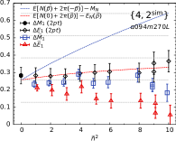
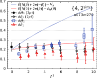
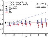
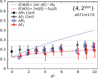
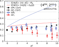
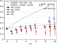
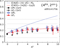
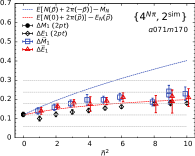
Figure 10: Estimates, in lattice units, of $\Delta M_{1}$ (black filled circles) and $\Delta E_{1}$ (open black diamonds) from fits to the two-point function for four ensembles in the order $a094m270L$, $a073m270$ , $a091m170L$ and $a071m170$ in each row. Each panel also shows the values of $\Delta{\widetilde{M}}_{1}$ (open blue squares) and $\Delta{\widetilde{E}}_{1}$ (open red triangles) from the $\{4,2^{\rm sim}\}$ (top row) and the $\{4^{N\pi},2^{\rm sim}\}$ (bottom row) fits to the vector three-point functions. The mass gaps of the noninteracting $N(\bm{q})2\pi(-\bm{q})$ and $N(\bm{0})2\pi(-\bm{q})$ states are shown by the dotted blue and red lines. The horizontal dotted black lines show the masses of $1,2,\ldots$ pions.

XII Electric and Magnetic Form Factors

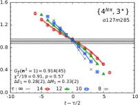
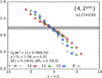
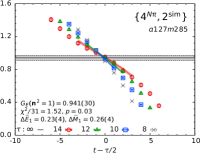
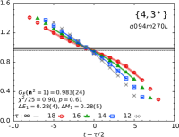
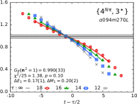
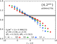
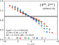
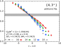
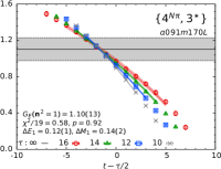
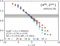
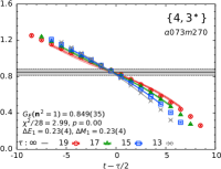
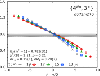
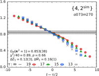
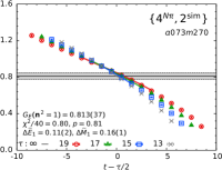
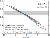
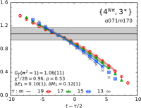
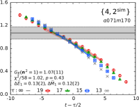
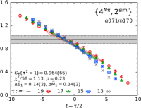
Figure 28: $G_{E}({\bm{n}}=(1,0,0))$, obtained from $\Im V_{i}$ (see Eq. (26)) plotted versus the shifted operator insertion point $t-\tau/2$. The rest is the same as in Fig. 23.

To obtain the electric and magnetic form factors, we analyze the three sets of correlators, $\Re V_{4}$, $\Im V_{i}$ and $\Re V_{i}$ defined in Eqs. (25)–(27) using four strategies $\{4,3^{\ast}\}$, $\{4^{N\pi},3^{\ast}\}$, $\{4,2^{\rm sim}\}$ and $\{4^{N\pi},2^{\rm sim}\}$ to remove ESC. In the $\{2^{\rm sim}\}$ fits to the three-point functions, all three correlators are fit simultaneously with common $\Delta{\widetilde{M}}_{1}$ and $\Delta{\widetilde{E}}_{1}$. Only the ground state parameters are taken from the two-point function. Fits with different strategies are illustrated in Figs. 27, 28 and 29 using the lowest momentum transfer (${\bm{n}}^{2}=1$) data that have significant ESC and a good statistical signal, and the fits are stable with respect to variations in $\tau$ and $t_{\rm skip}$. The $\chi^{2}/$dof of the fits and the values of $\Delta M_{1}$ and $\Delta E_{1}$ entering in the fits to the three-point functions (or $\Delta{\widetilde{M}}_{1}$ and $\Delta{\widetilde{E}}_{1}$ that are outcomes in the $\{2^{\rm sim}\}$ fits) are given in the legends. Note that for each strategy, the mass gaps in fits to the three correlation functions are the same since they either are taken from fits to two-point functions for the first two strategies or are outputs of simultaneous fits in the two $\{2^{\rm sim}\}$ cases.

The first issue we investigate is whether the excited states that contribute to these three correlators can be identified. The analog of the pion-pole dominance in the axial channel is vector-meson dominance, i.e., the vector current, $V_{\mu}(\bm{q})$, couples to the $\rho$-meson, the lowest excitation in the vector channel, and thus to the $2\pi(\bm{q})$ state. In this case, the dominant excited state contributing to $\Delta{\widetilde{M}}_{1}$ and $\Delta{\widetilde{E}}_{1}$ should be $N(\bm{q})2\pi(-\bm{q})$ (and/or $N(\bm{0})2\pi(\bm{0}))$ and $N(\bm{0})2\pi(\bm{q})$, respectively, where $2\pi(\bm{q})$ is a two pion state with total momentum $\bm{q}$.

In Fig. 10, the $\Delta{\widetilde{M}}_{1}$ and $\Delta{\widetilde{E}}_{1}$ from simultaneous $\{2^{\rm sim}\}$ fits are compared to the $\Delta M_{1}$ and $\Delta E_{1}$ from the $\{4\}$- and $\{4^{N\pi}\}$-state fits to the two-point functions and to the mass gaps expected for a specified state (dotted lines). Our criteria for identification of a state is when the $\Delta{\widetilde{M}}_{1}$ or $\Delta{\widetilde{E}}_{1}$ agree with the corresponding dotted line. We remind the readers that $\{4^{N\pi}\}$-state fits are also relevant for the vector channel because the mass gap of the $N(\bm{0})\pi(\bm{0})\pi(\bm{0})$ state is close to that for the $N(\bm{1})\pi(-\bm{1})$ state for our ensembles. The data exhibit the following features:

• The $\Delta{\widetilde{E}}_{1}$ (open red triangles) for the $170$ MeV ensembles are consistent with the energy of a noninteracting $N(\bm{0})2\pi(\bm{q})$ state shown by the red dotted line. This agreement is seen for both the $\{4,2^{\rm sim}\}$ and $\{4^{N\pi},2^{\rm sim}\}$ strategies.

• The $\Delta{\widetilde{E}}_{1}$ for the $270$ MeV ensembles lie between 1 and 2 times $M_{\pi}$. The closest association would be $N(\bm{q})\pi(\bm{0})$ or $N(\bm{0})\pi(\bm{q})$ or $N(\bm{q})2\pi(\bm{0})$ states but not the $N(\bm{0})2\pi(\bm{q})$ state shown by the red dotted line.

• The values of $\Delta{\widetilde{M}}_{1}$ (blue squares) lie much below the $N(\bm{q})2\pi(-\bm{q})$ state shown by the blue dotted line for the $270$ MeV ensembles, however, the difference decreases significantly in the data from the $170$ MeV ensembles. The increase with $\bm{q}$ also becomes similar in shape to that for $N(\bm{q})2\pi(-\bm{q})$.

• The $\Delta{\widetilde{M}}_{1}$ are similar to $\Delta{\widetilde{E}}_{1}$ for the $170$ MeV ensembles while they lie about $M_{\pi}/2$ above for the $270$ MeV ensembles. This behavior is very different from the axial case shown in Fig. 22.

• With $\{4^{N\pi},2^{\rm sim}\}$, the mass gap $\Delta{\widetilde{M}}_{1}\approx\Delta{\widetilde{E}}_{1}$ and comes close to $\Delta{E}_{1}$ used in $\{4^{N\pi},3^{\ast}\}$ for both $170$ MeV ensembles. Such an agreement in the mass gaps in the $\{4^{N\pi},2^{\rm sim}\}$ and $\{4^{N\pi},3^{\ast}\}$ strategies implies that they should give similar results.

These trends in $\Delta{\widetilde{M}}_{1}$ and $\Delta{\widetilde{E}}_{1}$ support vector meson dominance, i.e., the insertion of $2\pi(\bm{q})$ by the current, which we anticipate will become even more apparent on physical $M_{\pi}=135$ MeV ensembles. This is in analogy with pion-pole dominance with the axial current inserting $\pi(\bm{q})$ as inferred from Fig. 22. The values of $\Delta{\widetilde{M}}_{1}$ from the $M_{\pi}\approx 270$ MeV ensembles lying close to $2M_{\pi}$ suggest that the $N(\bm{0})2\pi(\bm{0})$ state and its tower also contribute on the ${\bm{p}}=0$ side of the operator.

Next, we investigated whether the data for $G_{E}$ from $\Im V_{i}$, which show large ESC as illustrated in Fig. 28 and similar to that seen in $\langle{\cal N}^{\dagger}A_{4}{\cal N}\rangle$, provide further insight on the identity of the excited states. We find that the $\chi^{2}/$dof of even the $\{4,3^{\ast}\}$ fits is not unreasonably large compared to the other strategies even though the values of $\Delta M_{1}$ and $\Delta E_{1}$ are significantly different. Overall, current data for $G_{E}^{V_{i}}$ do not help us decide which excited states give the dominant contribution.

An important feature in the ESC fits shown in Figs. 27 and 29 in Appendix G is that while the differences in the mass gaps between the four strategies are large, the variation in results for $G_{E}^{V_{4}}$ and $G_{M}^{V_{i}}$ is $\lesssim 5\%$. The smallness of the variation is further highlighted in Figs. 12 and 14—all four estimates of the form factors are consistent within errors with the Kelly parameterization of the experimental data.

We base our choice of which strategy to choose for presenting the final results on the trends in the mass gaps illustrated in Fig. 10. The first is the growing agreement between $\Delta{\widetilde{M}}_{1}$ and $\Delta{\widetilde{E}}_{1}$ in the $\{4^{N\pi},2^{\rm sim}\}$ data. Next, their agreement with the $\Delta{M}_{1}$ and $\Delta{E}_{1}$ from the $\{4^{N\pi}\}$ fits. Last, $\Delta{\widetilde{M}}_{1}\approx 2M_{\pi}$ suggests that the lowest excited state $N(0)\pi(0)\pi(0)$ also contributes. These trends suggest that the $\{4^{N\pi},2^{\rm sim}\}$ and $\{4^{N\pi},3^{\ast}\}$ strategies should give similar results for the form factors. Thus we will choose between these when presenting the final results.

Results for the renormalized form factors from the four strategies are given in Tables 22, 23, and 24. The $\chi^{2}/$dof of the fits used to remove the ESC are reasonable in most cases. The errors are the smallest in the $\{4,3^{\ast}\}$ data, and are large for many of the large $Q^{2}$ points from the $\{4,2^{\rm sim}\}$ and the $\{4^{N\pi},2^{\rm sim}\}$ fits. For this reason, we choose fits to the smallest six $Q^{2}$ points for calculating the charge radii.

A comparison of the form factors, and the errors in them, among the four strategies is shown in Fig. 11 for the five large volume ensembles. For each strategy, the full data from the seven ensembles are shown in Figs. 12, 13 and 14. The $G_{E}^{V_{i}}$ show significant variation between the strategies, with the $\{4,2^{\rm sim}\}$ data being closest to the Kelly curve. Part of this observed variation is a result of a poorer statistical signal and part due to less control over ESC. For these reasons, we do not include $G_{E}^{V_{i}}$ in our final analysis; however, this channel influences the extraction of $\Delta{\widetilde{M}}_{1}$ and $\Delta{\widetilde{E}}_{1}$ from the simultaneous $\{2^{\rm sim}\}$ fits.

For the two cases with the best signal, $G_{E}$ from $\Re V_{4}$ and $G_{M}$ from $\Re V_{i}$, we make the following observations from Fig. 11 using the Kelly curve as a benchmark and to guide the eye:

• No significant difference is observed between the data from the two simultaneous fits, $\{4,2^{\rm sim}\}$ versus $\{4^{N\pi},2^{\rm sim}\}$, i.e., the differences in the ground state parameters used do not significantly affect the results. On the four largest $Q^{2}$ points, the errors are large in many cases, but the overall shape of the data is similar for all four strategies.

• Results for $G_{E}^{V_{4}}$ and $G_{M}^{V_{i}}$ lie close to the Kelly parameterization for all four strategies, with the $\{4^{N\pi},3^{\ast}\}$ data plotted versus $Q^{2}/M_{N}^{2}$ showing the best agreement.

• All four strategies give consistent results on the $M_{\pi}\approx 270$ MeV ensembles.

• In Fig. 11, one can notice (i) a small spread among the four strategies in $G_{E}^{V_{4}}$ on the $M_{\pi}\approx 170$ MeV ensembles, (ii) a small upward movement of data from $a091m170L$ to $a071m170$, and (iii) the $\{4,3^{\ast}\}$ and both $\{2^{\rm sim}\}$ data on $a\approx 0.07$ fm ensembles lie above the Kelly curve.

• The $G_{M}^{V_{i}}$ data also move upwards from $a091m170L$ to $a071m170$. The $\{4,3^{\ast}\}$ strategy data lie below others on the two smallest $Q^{2}$ points.

• The data plotted versus $Q^{2}$ show some dependence on $a$ and/or $M_{\pi}^{2}$, whereas when plotted versus $Q^{2}/M_{N}^{2}$, no significant dependence on either $a$ or $M_{\pi}^{2}$ is observed, and the agreement with the Kelly curve is better. The size of the observed difference among the data plotted versus $Q^{2}$ or $Q^{2}/M_{N}^{2}$ can be accounted for by discretization errors. Assuming that there is a cancellation of these in the analysis versus the dimensionless quantity $Q^{2}/M_{N}^{2}$, we choose it for presenting our final results.

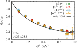
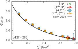
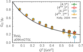
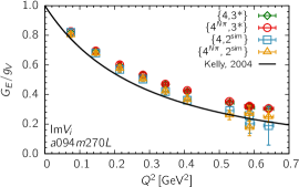
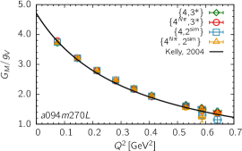
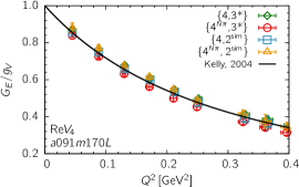
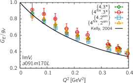
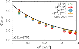
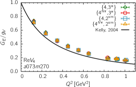
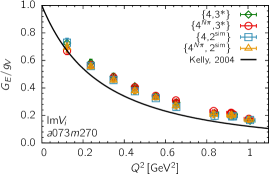
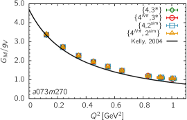
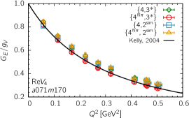
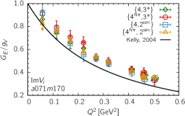
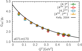
Figure 11: Each panel shows a comparison between the renormalized form factors $G_{E}^{\Re V_{4}}$ (left), $G_{E}^{\Im V_{i}}$ (middle), and $G_{M}^{\Re V_{i}}$ (right) obtained using four strategies and plotted versus $Q^{2}$ in GeV². The labels specify the strategy used to remove the ESC, and the ensemble ID. The solid black line shows the Kelly fit to the experimental data.

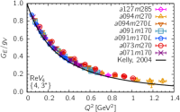
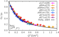
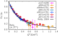
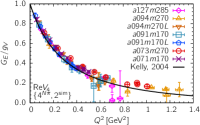
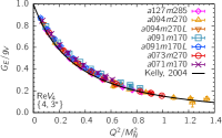
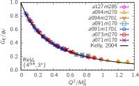
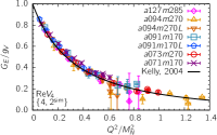
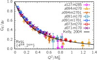
Figure 12: $G_{E}(Q^{2})$ from $\Re V_{4}$ plotted versus $Q^{2}$ in GeV² (top panels) and versus $Q^{2}/M_{N}^{2}$ (bottom panels). Each panel shows the data for the seven ensembles, and each row compares the four strategies used to remove ESC.

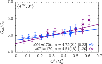
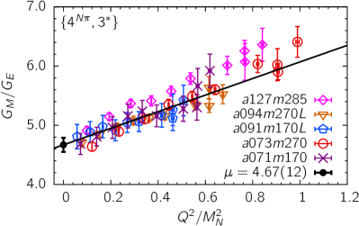
Figure 15: A linear fit to the smallest six $Q^{2}$ points for $G_{M}/G_{E}$ from the $a091m170L$ and $a071m170$ ensembles obtained with the $\{4^{N\pi},3^{\ast}\}$ strategy. The intercept at $Q^{2}=0$ gives $\mu^{u-d}$. The left panel shows separate fits to the two ensembles and the right to the combined data. Also shown, for comparison, in the right panel are the data from the other three larger volume $M_{\pi}\sim 270$ MeV ensembles.

	$\langle r_{E}^{2}\rangle|_{\rm dipole}$				$\langle r_{E}^{2}\rangle|_{z^{3}}$
Ensemble	$\{4,3^{\ast}\}$	$\{4^{N\pi},3^{\ast}\}$	$\{4,2^{\text{sim}}\}$	$\{4^{N\pi},2^{\text{sim}}\}$	$\{4,3^{\ast}\}$	$\{4^{N\pi},3^{\ast}\}$	$\{4,2^{\text{sim}}\}$	$\{4^{N\pi},2^{\text{sim}}\}$
$a127m285$	0.738(28)	0.773(27)	0.778(36)	0.777(38)	0.734(30)	0.768(30)	0.782(39)	0.778(43)
$a094m270$	0.698(37)	0.704(20)	0.705(49)	0.706(48)	0.656(52)	0.699(32)	0.692(62)	0.711(63)
$a094m270L$	0.682(22)	0.734(19)	0.698(22)	0.684(23)	0.669(24)	0.737(25)	0.701(25)	0.674(26)
$a091m170$	0.740(27)	0.891(32)	0.767(36)	0.728(32)	0.726(41)	0.969(77)	0.847(86)	0.772(98)
$a091m170L$	0.768(28)	0.902(54)	0.809(40)	0.784(38)	0.737(43)	0.893(79)	0.880(83)	0.76(10)
$a073m270$	0.643(23)	0.681(19)	0.667(25)	0.664(24)	0.625(26)	0.662(25)	0.712(33)	0.710(33)
$a071m170$	0.747(42)	0.854(43)	0.737(29)	0.712(25)	0.666(76)	0.834(96)	0.883(96)	0.72(11)
	$\langle r_{M}^{2}\rangle|_{\rm dipole}$				$\langle r_{M}^{2}\rangle|_{z^{3}}$
Ensemble	$\{4,3^{\ast}\}$	$\{4^{N\pi},3^{\ast}\}$	$\{4,2^{\text{sim}}\}$	$\{4^{N\pi},2^{\text{sim}}\}$	$\{4,3^{\ast}\}$	$\{4^{N\pi},3^{\ast}\}$	$\{4,2^{\text{sim}}\}$	$\{4^{N\pi},2^{\text{sim}}\}$
$a127m285$	0.582(22)	0.613(23)	0.627(29)	0.624(29)	0.569(33)	0.627(34)	0.672(34)	0.654(35)
$a094m270$	0.507(25)	0.505(19)	0.544(29)	0.536(26)	0.565(36)	0.623(36)	0.634(31)	0.657(37)
$a094m270L$	0.544(19)	0.613(19)	0.564(18)	0.558(17)	0.592(34)	0.642(34)	0.576(35)	0.568(34)
$a091m170$	0.562(23)	0.691(39)	0.592(26)	0.615(29)	0.77(11)	1.00(11)	0.765(86)	0.743(95)
$a091m170L$	0.630(29)	0.817(52)	0.610(27)	0.678(30)	0.61(11)	0.88(11)	0.55(10)	0.66(11)
$a073m270$	0.495(18)	0.514(16)	0.509(20)	0.522(18)	0.527(40)	0.545(40)	0.613(26)	0.636(36)
$a071m170$	0.562(31)	0.679(37)	0.581(25)	0.582(23)	0.71(12)	0.85(11)	0.89(10)	0.83(11)
	$\langle\mu\rangle|_{\rm dipole}$				$\langle\mu\rangle|_{z^{3}}$
Ensemble	$\{4,3^{\ast}\}$	$\{4^{N\pi},3^{\ast}\}$	$\{4,2^{\text{sim}}\}$	$\{4^{N\pi},2^{\text{sim}}\}$	$\{4,3^{\ast}\}$	$\{4^{N\pi},3^{\ast}\}$	$\{4,2^{\text{sim}}\}$	$\{4^{N\pi},2^{\text{sim}}\}$
$a127m285$	4.558(51)	4.696(64)	4.753(84)	4.730(82)	4.538(56)	4.712(71)	4.823(89)	4.771(86)
$a094m270$	4.252(84)	4.249(76)	4.421(94)	4.421(93)	4.343(67)	4.452(72)	4.542(73)	4.558(75)
$a094m270L$	4.369(41)	4.571(57)	4.444(44)	4.422(41)	4.419(47)	4.578(61)	4.441(53)	4.426(47)
$a091m170$	4.177(55)	4.598(95)	4.303(71)	4.359(72)	4.321(83)	4.749(54)	4.445(64)	4.474(77)
$a091m170L$	4.323(64)	4.717(99)	4.275(57)	4.494(83)	4.311(78)	4.735(85)	4.224(72)	4.484(84)
$a073m270$	4.273(52)	4.332(52)	4.307(65)	4.371(58)	4.301(71)	4.374(75)	4.487(70)	4.550(72)
$a071m170$	4.200(78)	4.526(96)	4.230(70)	4.286(74)	4.281(82)	4.560(75)	4.455(79)	4.469(80)

Table 9: Results for the isovector electric charge radius squared $\langle r_{E}^{2}\rangle$ (top); magnetic charge radius squared, $\langle r_{M}^{2}\rangle$ (middle); and magnetic moment, $\mu^{p}-\mu^{n}$ (bottom), for the seven ensembles obtained using the dipole and the $z^{3}$ parameterization of the $Q^{2}$ behavior. These fits were made keeping the smallest six $Q^{2}\neq 0$ points. In fits to $G_{M}$, we included the point $G_{M}(0)/g_{V}$, obtained by linearly extrapolating $G_{E}/G_{M}$ to $Q^{2}=0$, as a prior with width $0.2$. Data are compared for the four strategies ($\{4,3^{*}\}$, $\{4^{N\pi},3^{\ast}\}$, $\{4,2^{\text{sim}}\}$ and $\{4^{N\pi},2^{\text{sim}}\}$) for controlling ESC (see Appendix A). Dipole estimates are not included in the final results as explained in the text.

As mentioned above, the analog of the PCAC relation for the electromagnetic form factors is the conserved vector charge, i.e., $\lim_{Q^{2}\to 0}G_{E}(Q^{2})\equiv g_{V}=1/Z_{V}$. Since $g_{V}$ from the forward matrix element has $O(1\%)$ excited-state effect as shown in Fig. 2, one could use it to pick the best strategy, i.e., the one for which the extrapolation of $G_{E}(Q^{2})$ to $Q^{2}=0$ using the $z^{2}$ or Padé fit is most consistent with $g_{V}$. However, data from all four strategies shown in Figs. 12 and 14, are consistent within expected lattice artifacts with the Kelly parameterization, so this check does not help in picking among the strategies.

The reduction in scatter in the form factors under variation in $a$ and $M_{\pi}$ when plotted versus $Q^{2}/M_{N}^{2}$ is consistent with the analysis of clover-on-HISQ data presented in Ref. Jang et al. (2020b), where results by other collaborations carried out at or near the physical pion mass were also reviewed. On the other hand, the improvement in agreement with the Kelly curve of the clover-on-clover data presented here is striking. (See in particular the $\{4^{N\pi},3^{\ast}\}$ strategy data plotted versus $Q^{2}/M_{N}^{2}$ in Figs. 12 and 14.) Beyond the fact that the clover-on-clover formulation is unitary, the only substantial change in the lattice methodology we have made over the clover-on-HISQ calculations is the random parity transformation (see Eq. (14) in Sec. III) on all the lattices Yoon et al. (2016, 2017). Symmetry under parity plays an important role in constraining the excited states that should contribute; for example it disallows the $N(0)\pi(0)$ state. So, while we expect improvement in the precision with which correlation functions or contributions that should be zero under parity transformation are indeed zero, the level of improvement in agreement with the Kelly parameterization calls for further study.

For the $\{4,3^{\ast}\}$ strategy, the data in Fig. 11 for $G_{E}(Q^{2})$ lie above the Kelly curve and the low $Q^{2}$ points of $G_{M}(Q^{2})$ lie below. This behavior is in accord with the deviations pointed out in Ref. Jang et al. (2020b). The data with the $\{4^{N\pi},3^{\ast}\}$ strategy are more consistent with the Kelly result. We hypothesize on the basis of the observed improvement with the Kelly curve, the behavior of the mass gaps shown in Fig. 10, and the vector meson dominance model that the low lying multihadron excitations contribute. While significantly more data, especially on $M_{\pi}\approx 135$ MeV ensembles, are needed to validate this conjecture, we will select between $\{4^{N\pi},3^{\ast}\}$ and $\{4^{N\pi},2^{\rm sim}\}$ strategies for presenting results in this paper. Of these two strategies, the statistical precision of the current data is better for $\{4^{N\pi},3^{\ast}\}$ and it has the advantage of including three states in the fit. On the other hand $\{2^{\rm sim}\}$ is, statistically, better motivated if the same set of states contribute to the three correlation functions. For the time being, we will continue to analyze all four strategies since it is instructive to explore the differences.

The errors in the current lattice data are much larger than in the Kelly parameterization of the experimental data and cover a smaller range in $Q^{2}$. It will be some time before lattice data reach the precision of experiments even in the range $0.04<Q^{2}<1$ GeV². Nevertheless, we regard the consistency of our results with the Kelly curve an important and necessary step in demonstrating control over all systematic uncertainties in the calculations of form factors. The main thrust of future improvements will be on increasing the statistics, designing better nucleon interpolating operators to further control ESC, extending the calculation to more values of $a$ and $M_{\pi}$ to confirm the observed lack of dependence on them, and obtaining data at smaller values of $Q^{2}$.

Having obtained $G_{E}(Q^{2})$ and $G_{M}(Q^{2})$ from the four strategies to control ESC, we again parameterize the $Q^{2}$ dependence using the dipole, $z$-expansion and Padé fits. From these fits, we extract the electric and magnetic isovector charge radii squared, $\langle r_{E}^{2}\rangle$ and $\langle r_{M}^{2}\rangle$, and the magnetic moment $\mu$. These data are given in Table 9 and exhibit two noteworthy features: (i) the estimates with $\{4^{N\pi},3^{\ast}\}$ are larger, and (ii) the intercept at $Q^{2}=0$ of fits to $G_{M}/g_{V}$ shows the beginning of a flare-out, especially for $z$-expansion fits with sum rules. This second feature suggests that $Q^{2}=0$ is already at the edge of reliability of extrapolation of the fits to our data, which have $Q^{2}_{\rm min}\gtrsim 0.04$ GeV².

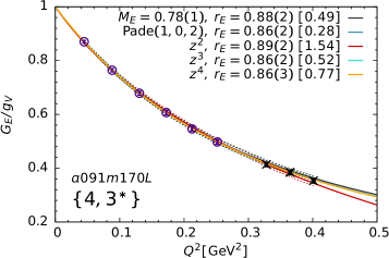
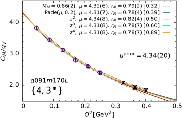
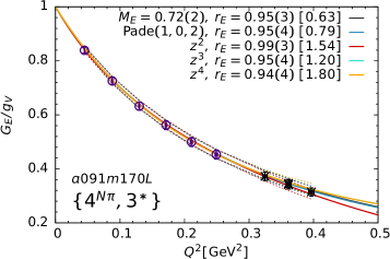
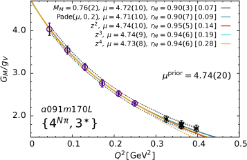
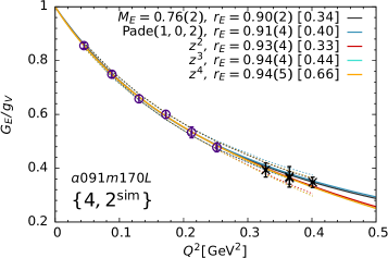
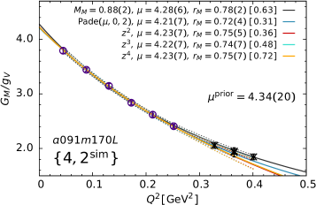
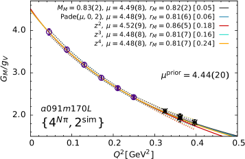
Figure 30: Data for the renormalized electric (left) and magnetic (right) form factors from the $a091m170L$ ensemble. All fits are made to the lowest six $Q^{2}$ points (open circles) and the remaining four points not fit are shown by the symbol cross. Error bands are shown only over the range of the data for clarity. The prior and its width, $\mu^{\rm prior}$, used in the fits to $G_{M}$ is given in each panel and explained in the text. The top line of the labels gives the results of the dipole fit ($M_{E}$, $\langle r_{E}\rangle$) or ($M_{M}$, $\mu$ and $\langle r_{M}\rangle$). Lines 2–5 give $\langle r_{E}\rangle$ or ($\mu$ and $\langle r_{M}\rangle$) from the $P_{2}$ Padé and the $z^{\{2,3,4\}}$ fits. In each case, the $\chi^{2}$/dof of the fits are given within the square brackets. The four rows show data from the four strategies $\{4,3^{\ast}\}$, $\{4^{N\pi},3^{\ast}\}$, $\{4,2^{\rm sim}\}$ and $\{4^{N\pi},2^{\rm sim}\}$ defined in the text.

In Ref. Jang et al. (2020b), we had shown that the ratio $G_{E}/G_{M}$ exhibits a linear behavior versus $Q^{2}$ and had used it to get an estimate of $G_{M}(Q^{2}=0)=\mu$. The clover-on-clover data presented in this study confirms this behavior as illustrated in Fig. 15 for the $a091m170L$ and $a071m170$ ensembles. So we use this value of $G_{M}(Q^{2}=0)/g_{V}$ as a prior in the fits to $G_{M}(Q^{2})/g_{V}$. The error in it is $\lesssim 0.2$ for all ensembles, so we select 0.2 for the width. Setting the width to 0.3 changes the estimates by $\lesssim\sigma/3$ for both $\mathop{\langle r_{M}^{2}\rangle}\nolimits$ and $\mu$. Overall, the use of the prior stabilizes the fits near $Q^{2}=0$, but does not change the results for $\mathop{\langle r_{M}^{2}\rangle}\nolimits$ or $\mu$ significantly. The dipole, Padé and $z$-expansion fits for the four strategies are illustrated in Figs. 30 and 31) in Appendix G for the $a091m170L$ and $a071m170$ ensembles, respectively. The values of $\mathop{\langle r_{E}^{2}\rangle}\nolimits,\ \mathop{\langle r_{M}^{2}\rangle}\nolimits,\ \mu$ obtained, and the prior used, are given in the labels. These fits are made to the six smallest $Q^{2}$ points since the errors are large in some of the higher $Q^{2}$ data. For completeness, we state that the results of fits to all ten points are essentially the same.

Two important points: first, the current data (six or ten values of $Q^{2}$) can be fit by the $z^{2}$ and $z^{3}$ truncations and $z^{4}$ is an overparameterization. We note a change between $z^{2}$ and $z^{3}$ and reasonable stability between $z^{3}$ and $z^{4}$. Thus all subsequent results are with fits using the $z^{3}$ truncation. Second, the two Padé fits give overlapping results, and the $P(g,1,3)$ is again an overparameterization.

To obtain the continuum limit values for $\mathop{\langle r_{E}^{2}\rangle}\nolimits$, $\mathop{\langle r_{M}^{2}\rangle}\nolimits$ and $\mu$, the CCFV fits to the data given in Table 9 are discussed in Sec. XIII.5.

XIII Final results from the chiral-continuum-finite-volume fits

In this section, we examine the dependence of the isovector charges, $g_{A,S,T}^{u-d}$, the axial charge radius $\langle r_{A}^{2}\rangle$, the induced pseudoscalar charge $g_{P}^{\ast}$, the pion-nucleon coupling $g_{\pi NN}$, the electric and magnetic charge radii, $\langle r_{E}^{2}\rangle$ and $\langle r_{M}^{2}\rangle$, and the magnetic moment $\mu^{u-d}$ on the lattice spacing $a$, pion mass $M_{\pi}$, and the lattice size parameter $M_{\pi}L$. The data are shown in Figs. 32–39 in Appendix H along with the CCFV fit results as pink bands. In cases for which the largest variation is versus $M_{\pi}^{2}$, we also show, for comparison, the result of just a chiral fit by a gray band. The more these two bands overlap, the more dominant is the chiral correction.

The overall framework of the CCFV analysis is as follows. A simultaneous CCFV fit in the three variables is made to get the results at the physical point defined as $M_{\pi}=135$ MeV, $a=0$ and $M_{\pi}L=\infty$. With seven data points, we can only include leading order corrections in each variable to avoid overparameterization. Keeping just the leading terms, we cannot directly assess a systematic error associated with possible higher-order corrections to the CCFV ansatz. What we do evaluate is whether the final error estimate from the simultaneous CCFV fit is conservative in comparison to the observed change under extrapolation in each parameter. In particular, for each quantity, we compare the change between the data from the ensemble closest to the physical point and the extrapolated value. For example, when discretization errors are dominant, we compare the difference between data at $a071m170$ and the extrapolated value with the error estimate from the CCFV fit to determine if the latter is conservative enough.

In all cases, the discretization corrections are taken to be linear in $a$ as our calculation (lattice action and operators) is not fully $O(a)$ improved.

To evaluate possible finite volume corrections in a given observable, we compare the data on the two pairs of ensembles $\{a094m270,a094m270L\}$ and $\{a091m170,a091m170L\}$. Second, we also compare outputs of chiral-continuum (CC) fits to the five larger volume data with CCFV fits to the seven points, and check for overparameterization. Differences between the two fits, if significant in comparison to the quoted error, are evaluated for whether an additional systematic uncertainty should be assigned. Overall, finite-volume corrections are observed to be small for $M_{\pi}L>4$.

The analysis so far has been carried out with a number of strategies for removing ESC in the various quantities. As already discussed, the overriding uncertainty in the final analysis comes from whether the low-lying $N\pi$ or $N\pi\pi$ states are relevant and included. Including them significantly impacts the estimates from the $M_{\pi}\approx 170$ MeV ensembles and thus the chiral extrapolation. In many cases the errors in the $\approx 170$ MeV data are much larger than in the $M_{\pi}\approx 270$ MeV points. Thus, their weight in the CCFV fits is small. This is a serious limitation. In subsequent sections, we will discuss this and other issues on a case-by-case basis, and provide our reasons for picking the strategy used to present the final results and the assessment of the need for an additional systematic uncertainty.

XIII.1 The CCFV extrapolation for $g_{A,S,T}^{u-d}$

The leading order CCFV fit ansatz used for all three isovector charges is

$$g(a,M_{\pi},M_{\pi}L)=c_{1}+c_{2}a+c_{3}M_{\pi}^{2}+c_{4}\frac{M_{\pi}^{2}e^{-M_{\pi}L}}{\sqrt{M_{\pi}L}}\,.$$ (41)

Results from these CCFV and CC ($c_{4}$ set to zero) fits to $g_{A,S,T}^{u-d}$ are summarized in Table 10 and the CCFV fits are shown in Figs. 32, 33 and 34 in Appendix H. Overall, these data indicate possible finite-volume corrections in $g_{A}^{u-d}$, but no significant effect is observed in $g_{S}^{u-d}$ or $g_{T}^{u-d}$. Below, just before Eq. (42), we also discuss the change in results (i) on assuming that the discretization errors begin at $O(a^{2})$, i.e., replacing the term $c_{2}a$ by $c_{2}a^{2}$, and (ii) without any discretization error term.

All averages presented in this section are averages weighted by the inverse square of the errors. In most cases the $\chi^{2}$ of the different fits whose results we average are very similar, so the averages constructed using AIC weights are also the same. Furthermore, both of these are also consistent with unweighted averages. We caution the reader that, for brevity, we use the term average to denote averages weighted by the inverse square of the errors.

We note a number of systematic shifts of $O(0.03)$ in results summarized in Table 10, which, while smaller than the individual total analysis errors in most cases, need to be addressed. These are (i) between the two renormalization methods ${\rm Z}_{1}$ and ${\rm Z}_{2}$, (ii) between the CC and CCFV fits and (iii) the variation between the various strategies.

The two methods of renormalization, ${\rm Z}_{1}$ and ${\rm Z}_{2}$, are equally well motivated, however, as discussed in Sec. VIII.1, and the errors in the renormalization constants are better controlled with ${\rm Z}_{1}$ for $g_{S}$ and with ${\rm Z}_{2}$ for $g_{A}$ and $g_{T}$. We, therefore average the $g_{S}$ values obtained with ${\rm Z}_{1}$, given in Table 10 and specified below, and $g_{A}$ and $g_{T}$ with ${\rm Z}_{2}$. To account for the difference in results obtained using ${\rm Z}_{1}$ versus ${\rm Z}_{2}$, we assign an additional systematic uncertainty for all three charges.

Second, comparing the CCFV and CC estimates, there is a notable difference only in $g_{A}^{u-d}$, which we discuss below. For $g_{S}^{u-d}$ and $g_{T}^{u-d}$, the CCFV fits have slightly larger errors but in most cases the reduction in $\chi^{2}$ is not sufficient to warrant including the finite volume correction term by the Akaike criteria. As they are consistent, we present the average of the CC and CCFV results.

On the third issue, for $g_{S}^{u-d}$ and $g_{T}^{u-d}$, the two $\{2^{\rm free}\}$ strategies yield an unexpectedly large $\Delta{\widetilde{M}}_{1}$. A larger value is expected in a two-state fit, i.e., it constitutes an effective mass gap representing the contribution of all excited states. Including a third state improves the estimate for $\Delta M_{1}$. Therefore, as discussed in Sec. VIII, we will choose the final results from the strategies that use a three-state fit, $\{4,3^{\ast}\}$ and $\{4^{N\pi},3^{\ast}\}$. The axial charge $g_{A}^{u-d}$ requires a more extensive analysis with respect to ESC that is presented below.

$\bm{g_{A}^{u-d}}$: The axial charges, summarized in Table 10 for the various strategies considered, are obtained in two different ways: (i) from the forward matrix element, which for the $\{4,3^{\ast}\}$ and $\{4^{N\pi},3^{\ast}\}$ strategies are given in rows one and eight, and (ii) by extrapolating the form factor $G_{A}(Q^{2})$ to $Q^{2}=0$. To specify the parameterization used in the second case, we introduce a third symbol, $\{D\}$/$\{z^{2}\}$/$\{P_{2}\}$, to represent a dipole/$z^{2}$/$P(g,0,2)$ fit. For example $\{4^{N\pi},3^{\ast},{z}^{2}\}$ means form factors obtained using the $\{4^{N\pi},3^{\ast}\}$ strategy and extrapolated using the $z^{2}$ fit (the glossary in Appendix A describes the various fits). In many of the CCFV fits, the data show no significant finite volume correction, especially above $M_{\pi}L>4.0$. The effect is much smaller than the overall analysis error from the CCFV fit shown in Fig. 32 in Appendix H. So we also performed CC fits to data neglecting the two small volume ensembles, $a094m270$ and $a091m170$. These are labeled as $\{{\widehat{D}}\}$ or $\{{\widehat{z}}^{2}\}$ or $\{{\widehat{P}}_{2}\}$. Overall, the main issue that needs to be resolved in both ways is whether the $N({\bm{1}})\pi({-\bm{1}})$ state should be included in the analysis.

With the $\{4,3^{\ast}\}$ strategy (first seven rows in Table 10), the $\Delta M_{1}$ from a four-state fit is large, about $600$ MeV, and the $\tau\to\infty$ value for $g_{A}^{u-d}$ is smaller, about 5% below the experimental value. In this case, estimates from the forward matrix element (first row) and those using the dipole or $z^{2}$ or Padé parameterization of the form factors give consistent results. Comparison of these estimates from the $Q^{2}$ fits is shown in the two left panels in Fig. 9 for the two $M_{\pi}\sim 170$ MeV ensembles.

With the $\{4^{N\pi},3^{\ast}\}$ strategy [uses the $N({\bm{1}})\pi({-\bm{1}})$ as the lowest excited state as discussed in Sec. V], we find that the finite-volume correction term is negligible as shown by the CCFV fit to the $\{4^{N\pi},3^{\ast}\}$ data in Fig. 32. Comparing the results in rows 9-14, we note that the estimates with the dipole fit, $\{4^{N\pi},3^{\ast},D\}$, are smaller. The reason is that the dipole fit misses the lowest $Q^{2}$ point on the $M_{\pi}\approx 170$ MeV ensembles as illustrated in the middle panels in Fig. 9.

With the preferred $\{4^{N\pi},2^{\text{sim}}\}$ strategy, selected on the basis of satisfying the PCAC relation, only results from the extrapolation of the form factor are possible. Within errors, the estimates in each of the four columns in Table 10 are consistent, but two of the three $O(0.03)$ shifts discussed above (renormalization, and finite volume indicated by CCFV versus CC estimates) are manifest. We derive our best estimate as follows. The finite volume systematic is not well controlled, so we average the larger volume, $M_{\pi}L>4$, CC-fit values $\{4^{N\pi},2^{\text{sim}},{\widehat{z}}^{2}\}$ and the $\{4^{N\pi},2^{\text{sim}},{\widehat{P}}_{2}\}$. For renormalization, we choose the ${\rm Z}_{2}$ estimates as discussed in Sec. VIII.1. With these choices, our result is $g_{A}^{u-d}=1.32(5)$. The same selection procedure applied to the $\{4,3^{\ast}\}$ strategy gives $g_{A}^{u-d}=1.23(4)$. The large difference, $\sim 0.09$, makes it clear that establishing whether the low-mass $N\pi$ state(s) contribute is essential to the extraction of $g_{A}^{u-d}$.

Three systematic uncertainties, summarized in Eq. (42), are added to the above estimate. These are taken to be half the spread in the data in Table 10 as follows: For renormalization it is half the difference between the ${\rm Z}_{1}$ and ${\rm Z}_{2}$ values, i.e., 0.02. Half the spread in results between the strategies that include the $N\pi$ state when removing ESC gives 0.04. For finite volume corrections, half the difference between the CC and CCFV fit values gives 0.02. In all these averages and error estimates, we do not consider the dipole fit values since these fits miss the lowest $Q^{2}$ point on the $M_{\pi}\approx 170$ MeV ensembles. This is illustrated in the right panels in Fig. 9.

Overall, in the CCFV fits we note (i) there is tiny if any $a$ dependence in data from any of the strategies investigated; (ii) there is almost no dependence on $M_{\pi}^{2}$ for $\{4,3^{\ast}\}$ but a significant one in the strategies that include the $N\pi$ state; and (iii) there is an indication of a finite volume correction with the $\{4^{N\pi},2^{\text{sim}},z^{2}\}$ and $\{4^{N\pi},2^{\text{sim}},P_{2}\}$ strategies. Of these three changes, the largest effect is in the slope versus $M_{\pi}^{2}$ on including the $N\pi$ state. The contribution of the $N\pi$ state grows as $Q^{2}\to 0$ and $M_{\pi}\to 135$ MeV. Since $G_{A}(Q^{2})$ is analytical and monotonic in $Q^{2}$, we expect the influence of the $N\pi$ state to persist at $Q^{2}=0$ in the sense that the value of $g_{A}$ obtained directly at $Q^{2}=0$ from the forward matrix element calculated using the $A_{3}$ correlator must agree in the continuum limit with that extracted from a $z$-expansion (or Padé) fit to the form factor. Even though our data satisfy this check individually for both $\{4,3^{\ast}\}$ and $\{4^{N\pi},3^{\ast}\}$ strategies as shown in Table 10, the value of $g_{A}$, however, is different. The estimate from $\{4^{N\pi},3^{\ast}\}$ varies between $1.28(5)$ and $1.33(5)$. This is consistent with our final result, $g_{A}^{u-d}=1.32(6)$, and the error covers the $\{4^{N\pi},2^{\text{sim}},{\widehat{z}}^{2}\}$ and the $\{4^{N\pi},2^{\text{sim}},{\widehat{P}}_{2}\}$ estimates.

We consider $\{4^{N\pi},2^{\text{sim}},{\widehat{z}}^{2}\}$ and $\{4^{N\pi},2^{\text{sim}},{\widehat{P}}_{2}\}$ as two models because, up to some reasonably small $Q^{2}$, both the fixed order $z$-expansion and the Padé should give the same intercept in the limit of perfect data. The reason we take the weighted average and do not include the AIC weight is because the $\chi^{2}$ of both is abnormally small as discussed below.

$\bm{g_{S}^{u-d}}$: We neglect the results from the two $\{2^{\rm free}\}$ strategies, which are somewhat larger, because the associated $\Delta{\widetilde{M}}_{1}$ is larger than even that from the $\{4\}$ fit as discussed in Sec. VIII. Results from $\{4,3^{\ast}\}$ and $\{4^{N\pi},3^{\ast}\}$ overlap (see Fig. 3) and no significant finite-volume correction is observed. Thus we average estimates from the latter two strategies and the two fits, CCFV and CC, all with the ${\rm Z}_{1}$ renormalization method (see Sec. VIII.1). The result is q$g_{S}^{u-d}=1.06(9)$. Note that the error estimate covers the larger but neglected $\{2^{\rm free}\}$ values.

The most significant variation in the CCFV fits shown in Fig. 33 in Appendix H is versus $a$. The difference between the $a=0.071$ fm and the $a=0$ value is $\sim 0.12$, so we assign, in Eq. (42), an additional systematic uncertainty of 0.06 for possible incomplete accounting of the discretization error in the CCFV or CC fits. Estimates from the two renormalization methods show a difference of $\sim 0.04$, so we assign an additional systematic uncertainty of $0.02$.

$\bm{g_{T}^{u-d}}$: We again neglect the results from the two $\{2^{\rm free}\}$ fits for the same reason as for $g_{S}^{u-d}$. Similarly, we take the weighted average of the remaining four estimates in Table 10 with ${\rm Z}_{2}$ renormalization and get $g_{T}^{u-d}=0.97(3)$. The largest variation in the CCFV fits shown in Fig. 34 in Appendix H is versus $M_{\pi}^{2}$, with a possible $\sim 0.02$ difference between $M_{\pi}=170$ and the extrapolated 135 MeV value. This difference is covered by the overall analysis (CC or CCFV) error. There is also a $\approx 0.02$ difference between the two ES strategies (see Fig. 3), so we assign a $0.01$ uncertainty for possible additional ES effects. Last, the two renormalization methods give estimates that differ by $\sim 0.02$, so we assign an additional $0.01$ uncertainty due to it.

Remarks on discretization errors: The discretization correction in the CC and CCFV fit ansatz, Eq. (41), is taken to be linear in $a$ since our action and the axial operator are not fully $O(a)$ improved. We have also carried out the analysis with the errors starting at $O(a^{2})$, i.e., using $c_{2}a^{2}$ instead of $c_{2}a$ in Eq. (41) and assuming the linear in $a$ correction is negligible. The $\chi^{2}$ of the two sets of CCFV fits are essentially the same for all three charges. The corresponding estimates for the charges change to $g_{A}^{u-d}=1.34(4)$, $g_{S}^{u-d}=0.97(6)$ and $g_{T}^{u-d}=0.97(2)$. The reason for the smaller CCFV fit errors is that the range of extrapolation to the continuum limit is smaller in $a^{2}$. We keep the larger error estimates from fits with $c_{2}a$ but assign an additional discretization uncertainty of $0.02$ and $0.01$ for $g_{A}^{u-d}$ and $g_{T}^{u-d}$, respectively. The largest change in $g_{S}^{u-d}$ is with respect to $a$ and the error already assigned covers the variation between $c_{2}a$ and $c_{2}a^{2}$ fits.

We also show chiral fits (gray bands) for $g_{A}$ and $g_{T}$ in the middle panels of Figs 32 and 34. The reason for neglecting discretization and finite volume corrections is the observation that the data on the five large volume lattices do not show a significant dependence on $a$ or $M_{\pi}L$. In all cases, these results overlap with the CCFV values but have smaller errors. The similar $\chi^{2}$ suggests that the CCFV fits are overparameterized. Nevertheless, as discussed above, for the final results we quote the CC values and errors for $g_{A}$ and CCFV for $g_{S}$ and $g_{T}$.

Remarks on low $\chi^{2}$ values in CCFV fits: The $\chi^{2}$ of the two fits $\{4^{N\pi},2^{\text{sim}},{\widehat{z}^{2}}\}$ and $\{4^{N\pi},2^{\text{sim}},{\widehat{P}}_{2}\}$ used to get $g_{A}^{u-d}$ are essentially zero as given in Table 10. The following two factors could explain such $\chi^{2}\ll 1$: (i) the errors assigned to the data points are overestimated, and (ii) the fits are overparameterized. The first because the error in the multiplicative renormalization factor $Z_{A}$ is of the same size as the statistical error in $g_{A}^{\rm bare}$ (see Tables 3 and 4) and is neither normally distributed nor independent. The second because the discretization errors are small and including the $c_{2}$ term is an overparameterization. We have chosen to include it (CC fit) but do not construct an AIC weighted average due to the small $\chi^{2}$.

Within this framework, our final results are

Charge Value $$\delta$$ES Z FV

1.32(6) (4) (2) (2) (2)

1.06(9) (2) (6)

0.97(3) (1) (1) (1)

(42)

where the first error is the overall analysis uncertainty and $\delta$ES, $\delta$Z, $\delta a$, and $\delta$FV are the additional systematic uncertainties due to excited states, renormalization, discretization and finite volume artifacts. Combining these systematic errors in quadrature, our results are:

$$g_{A}^{u-d} = 1.32(6)(5)_{\rm sys}\,,$$

$$g_{S}^{u-d} = 1.06(9)(6)_{\rm sys}\,,$$

$$g_{T}^{u-d} = 0.97(3)(2)_{\rm sys}\,.$$ (43)

Even with our high statistics data, the errors in $g_{A}^{u-d}$ are much larger than in the experimental value $g_{A}^{u-d}=1.2764(1)$ Mendenhall et al. (2013); Brown et al. (2018); Mund et al. (2013). Estimates for $g_{S}^{u-d}$ and $g_{T}^{u-d}$ are consistent with results in Ref.  Gupta et al. (2018) obtained using the clover-on-HISQ formulation.

Strategy	$g_{A}^{u-d}|_{{\rm Z}_{1}}$ ($c_{4}=0$)	$g_{A}^{u-d}|_{{\rm Z}_{1}}$	$g_{A}^{u-d}|_{{\rm Z}_{2}}$ ($c_{4}=0$)	$g_{A}^{u-d}|_{{\rm Z}_{2}}$
{4,3*}	1.215(48) [0.26]	1.203(59) [0.31]	1.250(42) [0.18]	1.250(51) [0.24]
$\{4,3^{*},z^{2}\}$	1.194(44) [0.04]	1.200(52) [0.05]	1.230(39) [0.12]	1.242(46) [0.05]
$\{4,3^{*},{\widehat{z}^{2}}\}$	1.194(44) [0.02]		1.230(40) [0.14]
$\{4,3^{*},P_{2}\}$	1.184(46) [0.02]	1.191(56) [0.01]	1.221(41) [0.16]	1.239(49) [0.06]
$\{4,3^{*},{\widehat{P}_{2}}\}$	1.185(46) [0.00]		1.222(41) [0.23]
$\{4,3^{*},D\}$	1.183(42) [0.35]	1.206(48) [0.15]	1.217(36) [0.59]	1.248(42) [0.03]
$\{4,3^{*},{\widehat{D}}\}$	1.184(42) [0.05]		1.219(37) [0.13]
{$4^{N\pi}$,3*}	1.280(48) [0.11]	1.288(55) [0.12]	1.317(42) [0.14]	1.331(47) [0.03]
$\{4^{N\pi},3^{*},z^{2}\}$	1.274(52) [0.24]	1.289(61) [0.24]	1.307(48) [0.24]	1.328(55) [0.13]
$\{4^{N\pi},3^{*},{\widehat{z}^{2}}\}$	1.277(54) [0.24]		1.312(49) [0.15]
$\{4^{N\pi},3^{*},P_{2}\}$	1.272(57) [0.14]	1.273(69) [0.18]	1.308(53) [0.10]	1.316(62) [0.12]
$\{4^{N\pi},3^{*},{\widehat{P}_{2}}\}$	1.277(58) [0.20]		1.313(54) [0.10]
$\{4^{N\pi},3^{*},D\}$	1.222(49) [0.61]	1.262(56) [0.14]	1.256(43) [0.98]	1.303(50) [0.03]
$\{4^{N\pi},3^{*},{\widehat{D}}\}$	1.225(50) [0.01]		1.260(45) [0.18]
$\{4,2^{\text{sim}},z^{2}\}$	1.248(55) [0.84]	1.295(66) [0.56]	1.276(51) [1.07]	1.332(61) [0.52]
$\{4,2^{\text{sim}},{\widehat{z}^{2}}\}$	1.263(56) [0.05]		1.296(52) [0.04]
$\{4,2^{\text{sim}},P_{2}\}$	1.239(64) [0.91]	1.290(78) [0.78]	1.269(59) [1.12]	1.332(73) [0.75]
$\{4,2^{\text{sim}},{\widehat{P}_{2}}\}$	1.257(65) [0.07]		1.293(60) [0.05]
$\{4,2^{\text{sim}},D\}$	1.160(47) [1.50]	1.219(54) [0.35]	1.193(43) [2.33]	1.261(49) [0.27]
$\{4,2^{\text{sim}},{\widehat{D}}\}$	1.159(47) [0.06]		1.192(43) [0.49]
$\{4^{N\pi},2^{\text{sim}},z^{2}\}$	1.279(54) [0.68]	1.320(62) [0.34]	1.308(50) [1.04]	1.357(57) [0.37]
$\{4^{N\pi},2^{\text{sim}},{\widehat{z}^{2}}\}$	1.290(54) [0.00]		1.322(50) [0.26]
$\{4^{N\pi},2^{\text{sim}},P_{2}\}$	1.273(63) [0.73]	1.326(75) [0.38]	1.303(59) [1.07]	1.368(69) [0.38]
$\{4^{N\pi},2^{\text{sim}},{\widehat{P}_{2}}\}$	1.283(64) [0.00]		1.316(59) [0.23]
$\{4^{N\pi},2^{\text{sim}},D\}$	1.210(48) [1.14]	1.259(55) [0.27]	1.242(44) [1.90]	1.299(49) [0.27]
$\{4^{N\pi},2^{\text{sim}},{\widehat{D}}\}$	1.215(49) [0.02]		1.250(44) [0.43]
Strategy	$g_{S}^{u-d}|_{{\rm Z}_{1}}$ ($c_{4}=0$)	$g_{S}^{u-d}|_{{\rm Z}_{1}}$	$g_{S}^{u-d}|_{{\rm Z}_{2}}$ ($c_{4}=0$)	$g_{S}^{u-d}|_{{\rm Z}_{2}}$
$\{4,3^{\ast}\}$	1.068(68) [0.05]	1.052(92) [0.04]	1.101(96) [0.05]	1.09(12) [0.07]
$\{4^{N\pi},3^{\ast}\}$	1.062(93) [0.05]	1.06(11) [0.06]	1.10(11) [0.02]	1.10(13) [0.02]
{$4,2^{\text{free}}$}	1.056(52) [0.39]	1.086(63) [0.28]	1.081(82) [0.40]	1.118(92) [0.27]
{$4^{N\pi},2^{\text{free}}$}	1.100(52) [1.01]	1.157(61) [0.25]	1.120(82) [0.85]	1.186(91) [0.21]
Strategy	$g_{T}^{u-d}|_{{\rm Z}_{1}}$ ($c_{4}=0$)	$g_{T}^{u-d}|_{{\rm Z}_{1}}$	$g_{T}^{u-d}|_{{\rm Z}_{2}}$ ($c_{4}=0$)	$g_{T}^{u-d}|_{{\rm Z}_{2}}$
$\{4,3^{\ast}\}$	0.944(46) [0.06]	0.942(53) [0.08]	0.968(27) [0.03]	0.971(34) [0.03]
$\{4^{N\pi},3^{\ast}\}$	0.938(50) [0.14]	0.926(57) [0.13]	0.962(33) [0.15]	0.955(38) [0.17]
{$4,2^{\text{free}}$}	0.995(43) [0.15]	0.985(50) [0.15]	1.017(24) [0.26]	1.017(29) [0.35]
{$4^{N\pi},2^{\text{free}}$}	1.027(44) [0.22]	1.027(50) [0.29]	1.047(25) [0.46]	1.047(28) [0.61]

Table 10: Results for the renormalized $g_{A,S,T}^{u-d}$ after CC ($c_{4}=0$) and CCFV extrapolations using Eq. (41) for the various strategies used to remove the ESC listed in column one that are discussed in Secs. VIII and X, as well as in Appendix A. The results for $g_{A}^{u-d}$ labeled with additional $z^{2}$/$P_{2}$/$D$ use $g_{A}=G_{A}(Q^{2}=0)$ obtained by extrapolating $G_{A}(Q^{2})$ to $Q^{2}=0$ using these fits to all ten $Q^{2}\neq 0$ points (see glossary in Appendix A). The results in rows with ${\widehat{D}}$/${\widehat{z}}^{2}$/${\widehat{P}}_{2}$ are from CC fits to data excluding the small volume $a094m270$ and $a091m170$ ensembles. The $\chi^{2}$/dof of the CC and CCFV fits are given within the square brackets.

XIII.2 The CCFV extrapolation for the axial charge radius squared $\langle r_{A}^{2}\rangle$

The data given in Table 6 show no significant difference between the $\{4,3^{\ast}\}$ and $\{4^{N\pi},2^{\rm sim}\}$ strategies on the $M_{\pi}\approx 270$ MeV ensembles. However, there is a difference on the $M_{\pi}\approx 170$ MeV ensembles due to the inclusion of the $N\pi$ state. We have summarized our reasons for choosing the $\{4^{N\pi},2^{\rm sim}\}$ strategy for the analysis of the axial form factors $G_{A}$ and ${\widetilde{G}}_{P}$ in Sec. IX.1, and we will use it to obtain the quantities derived from them, $\langle r_{A}^{2}\rangle$, $g_{P}^{\ast}$, and $g_{\pi NN}$.

The CCFV ansatz used to fit $\langle r_{A}^{2}\rangle$,

$$r_{A}^{2}(a,M_{\pi},L) = c_{1}+c_{2}a+c_{3}M_{\pi}^{2}+c_{4}M_{\pi}^{2}\frac{e^{-M_{\pi}L}}{\sqrt{M_{\pi}L}}\,,$$ (44)

is the same as for the isovector charges given in Eq (41). Fits with the $\{4^{N\pi},2^{\rm sim},z^{2}\}$ strategy are shown in Fig. 35 and the results summarized in Table 11. We note a strong dependence on $M_{\pi}^{2}$ and a slight increase with both $M_{\pi}L$ and $a$. Most of the increase with $M_{\pi}L$ takes place for $M_{\pi}L<4$; therefore, we take the final result from the $\{4^{N\pi},2^{\rm sim},{\widehat{z}}^{2}\}$ analysis:

$$r^{2}_{A}|_{z^{2}}=0.428(53)(30)\ {\rm fm}^{2}\ \Rightarrow r_{A}|_{z^{2}}=0.65(4)(2)\ {\rm fm}\,,$$ (45)

where the second, systematic, uncertainty is the difference from the $\{4^{N\pi},2^{\rm sim},{\widehat{P}}_{2}\}$ value. This result is consistent with the $\{4^{N\pi},2^{\rm sim},z^{2}\}$ and $\{4^{N\pi},2^{\rm sim},P_{2}\}$ values, and the quoted error also covers the spread in the CCFV estimates from the $\{4^{N\pi},3^{\ast}\}$, $\{4,2^{\rm sim}\}$, $\{4^{N\pi},2^{\rm sim}\}$ strategies and both $z^{2}$ and $P_{2}$ fits.

Results for $\langle r_{A}^{2}\rangle$ using the dipole parameterization of the $Q^{2}$ behavior are significantly smaller than those from the $z^{2}$ or $P_{2}$ fits, and the $\chi^{2}$/dof is large in many cases. More important, these fits miss the low $Q^{2}$ points as illustrated in Fig. 9. So we do not include the dipole estimates in deriving the final results.

Our result, $r_{A}=0.65(4)(2)$ fm, is consistent with the three phenomenological/experimental values: (i) a weighted world average of (quasi)elastic neutrino and antineutrino scattering data Bernard, Veronique and Elouadrhiri, Latifa and Meißner, Ulf-G. (2002), (ii) charged pion electroproduction experiments Bernard, Veronique and Elouadrhiri, Latifa and Meißner, Ulf-G. (2002), and (iii) a reanalysis of the deuterium target data Meyer et al. (2016):

$$r_{A} =0.666(17){\rm fm}\ ({\cal M}_{A}=1.03(2){\rm GeV})\ [\nu,{\overline{\nu}}\ {\rm scattering}]\,,$$

$$r_{A} =0.639(10){\rm fm}\ ({\cal M}_{A}=1.07(2){\rm GeV})\ [{\rm Electroprod.}]\,,$$

$$r_{A} =0.68(16){\rm fm}\ \ ({\cal M}_{A}=1.00(24){\rm GeV})\ [{\rm Deuterium}]\,.$$ (46)

In this list, we do not quote the MiniBooNE value ${\cal M}_{A}=1.35(17)$ GeV ($r_{A}=0.506$ fm) Aguilar-Arevalo et al. (2010) as it is not the outcome of an analysis, but the best value that reproduces the double differential cross section for charged current quasielastic neutrino and antineutrino scattering data off carbon analyzed with a dipole ansatz and a relativistic Fermi gas model of nuclear interactions Smith and Moniz (1972). It will be interesting to see an update of the MiniBooNE analysis with our parameterization of $G_{A}(Q^{2})$ given in Eq. (55) and a more realistic model of nuclear interactions Lynn et al. (2019); Carlson et al. (2015).

ESC Strategy	$z^{2}$ ($c_{4}=0$)	$z^{2}$	$P_{2}$ ($c_{4}=0$)	$P_{2}$	dipole ($c_{4}=0$)	dipole
$\{4,3^{\ast}\}$	0.307(38) [0.27]	0.319(45) [0.29]	0.276(48) [0.36]	0.298(58) [0.33]	0.262(29) [1.58]	0.297(34) [0.78]
$\{4,3^{\ast}\}{\dagger}$	0.306(40) [0.51]		0.277(48) [0.70]		0.270(29) [1.41]
$\{4^{N\pi},3^{\ast}\}$	0.424(45) [0.34]	0.446(49) [0.10]	0.408(62) [0.17]	0.412(72) [0.23]	0.315(30) [2.75]	0.362(34) [0.46]
$\{4^{N\pi},3^{\ast}\}{\dagger}$	0.441(49) [0.07]		0.421(65) [0.06]		0.327(33) [1.53]
$\{4,2^{\text{sim}}\}$	0.413(47) [1.95]	0.450(53) [1.89]	0.375(75) [1.99]	0.434(90) [2.20]	0.228(25) [6.06]	0.281(28) [0.31]
$\{4,2^{\text{sim}}\}{\dagger}$	0.465(51) [0.42]		0.445(80) [0.57]		0.224(26) [2.01]
$\{4^{N\pi},2^{\text{sim}}\}$	0.399(49) [1.01]	0.439(55) [0.47]	0.366(80) [0.90]	0.437(93) [0.48]	0.244(27) [4.71]	0.283(29) [0.98]
$\{4^{N\pi},2^{\text{sim}}\}{\dagger}$	0.428(53) [0.33]		0.398(83) [0.31]		0.243(28) [2.04]

Table 11: Results for the axial charge radius $\langle r_{A}^{2}\rangle$ from (i) different strategies for removing ESC listed in column one (see Appendix A) and (ii) fits to the ten $Q^{2}\neq 0$ points for the axial form factor $G_{A}(Q^{2})$ using the $z^{2}$, $P_{2}$ Padé and the dipole parameterizations. The additional ${\dagger}$ in column one denotes results from CC fits with $c_{4}=0$, i.e., neglecting the small volume ($a094m270$ and $a091m170$) points. The $\chi^{2}$/dof of the $Q^{2}$ fits are given within the square brackets.

XIII.3 The CCFV extrapolation for $g_{P}^{\ast}$ and $g_{\pi NN}$

To perform the CCFV fit for $g_{P}^{\ast}$ given in Table 8, we use the ansatz

$$g_{P}^{\ast}(a,M_{\pi},M_{\pi}L)/g_{A}= d_{1}+d_{2}a+\frac{d_{4}}{M_{\pi}^{2}+0.88m_{\mu}^{2}}$$

$$+ d_{3}M_{\pi}^{2}+\frac{d_{5}M_{\pi}^{2}}{\sqrt{M_{\pi}L}}e^{-M_{\pi}L}\,,$$ (47)

where the leading behavior in $M_{\pi}^{2}$ is taken to be the pion-pole term evaluated at the momentum scale of the muon capture experiment Andreev et al. (2013, 2015). The data and fit in Fig. 35 in Appendix H show no significant dependence on either $a$ or $M_{\pi}L$ but a strong dependence on $M_{\pi}^{2}$. The result of the CCFV fit to the $\{4^{N\pi},2^{\rm sim}\}$ data is

$$g_{P}^{\ast} = 7.9(7)(9)_{\rm sys}\,,$$ (48)

where the second systematic uncertainty is half the change from the $a071m170$ point in the chiral extrapolation. The two methods for renormalization give overlapping results, so we do not assess an additional systematic uncertainty due to it. To underscore the importance of including the $N\pi$ state in the analysis of ESC, note that the analogous result with the $\{4,3^{\ast}\}$ strategy is $3.9(1.1)$.

Experimentally, ${\widetilde{G}}_{P}(Q^{2}=0.88m_{\mu}^{2})$ is determined from muon capture by a proton, $\mu^{-}+p\to\nu_{\mu}+n$ Andreev et al. (2013, 2015). Current estimates from the MuCap experiment Andreev et al. (2013, 2015), and from chiral perturbation theory Schindler et al. (2007); Bernard, Veronique and Elouadrhiri, Latifa and Meißner, Ulf-G. (2002) are

$$g_{P}^{\ast}|_{\rm MuCap} = 8.06(55)\,,$$

$$g_{P}^{\ast}|_{\chi{\rm PT}} = 8.29^{+0.24}_{-0.13}\pm 0.52\,,$$ (49)

respectively.

The CCFV fit to the pion-nucleon coupling $g_{\pi NN}$ data, also given in Table 8, was carried out using the ansatz given in the right-hand side of Eq. (44). The result of the fit, shown in Fig. 35 in Appendix H, is

$$g_{\pi NN} = 12.4(1.2)\,.$$ (50)

Again, the dominant dependence of the data is on $M_{\pi}^{2}$ but there is no significant change from the $a071m170$ value. The variation with the renormalization method is $\sim 0.3\sigma$. These are much smaller than the quoted $1\sigma$ error, so we do not assign an additional systematic uncertainty. For comparison, the result with the $\{4,3^{\ast}\}$ strategy that does not include the $N\pi$ state is $6.8(1.3)$.

To summarize, results for all three quantities, $\langle r_{A}^{2}\rangle$, $g_{P}^{\ast}$ and $g_{\pi NN}$ given in Eqs. (44), (48) and (50) come in reasonable agreement with phenomenological values with the $\{4^{N\pi},2^{\rm sim}\}$ strategy that is singled out on the basis of the axial form factors satisfying the PCAC relation.

XIII.4 Goldberger-Treiman relation and $F_{\pi}$

The Goldberger-Treiman (GT) relation predicts $g_{\pi NN}(1+\Delta)=M_{N}g_{A}/F_{\pi}$ as discussed in Sec. IX.1. Three of these quantities, $M_{N}$ (Table 15), $g_{A}$ (Table 4) and $F_{\pi}$ (Table 1), are calculated in this work. Data for the product $M_{N}g_{A}/F_{\pi}$, which is independent of the renormalization constant $Z_{A}$ and the lattice scale, are also given in Table 1 for each ensemble. The CCFV fits to these data for $M_{N}g_{A}/F_{\pi}$ and $F_{\pi}$ using the ansatz given in Eq. (44) are shown in Fig. 36 in Appendix H. The result for $M_{N}g_{A}/F_{\pi}$ depends, as expected, on the strategy used to determine $g_{A}$, and for the two extreme values for $g_{A}$ obtained from $\{4,3^{\ast}\}$ and $\{4^{N\pi},2^{\rm sim},z^{2}\}$ fits discussed in Sec. XIII.1, it is $=12.65(38)$ and $13.58(49)$, respectively. We also show the CCFV fit for $F_{\pi}$ in the bottom row of Fig. 36 and find $F_{\pi}=93.0(3.9)$ (96.1(3.6)) MeV with ${\rm Z}_{1}$ (${\rm Z}_{2}$) renormalization. These CCFV fits to the $F_{\pi}$ and $M_{N}g_{A}/F_{\pi}$ data show significant variation with $a$ and $M_{\pi}$. Thus, to improve precision more $\{a,M_{\pi},M_{\pi}L\}$ points are needed.

For comparison, using the experimental values, $g_{A}=1.2764$, $M_{N}=939$ MeV and $F_{\pi}=92.2$ MeV and ignoring the Goldberger-Treiman discrepancy $\Delta$ (see discussion in Sec. IX) give $\mathop{g_{\pi{NN}}}\nolimits=M_{N}g_{A}/F_{\pi}=13$. The phenomenological estimate obtained from the $\pi N$ scattering length analysis is $13.25(5)$ Navarro Pérez et al. (2017); Reinert et al. (2021); Baru et al. (2011).

		$\langle r_{E}^{2}\rangle$		$\langle r_{M}^{2}\rangle$		$\mu$
ESCfit	$Q^{2}$fit	CC	CCFV	CC	CCFV	CC	CCFV
$\{4,3^{*}\}$	$D$	0.633(60)[0.26]	0.658(75)[0.25]	0.479(48)[1.24]	0.579(67)[0.04]	3.78(12)[1.36]	3.95(15)[0.54]
	$P_{2}$	0.589(74)[0.07]	0.613(98)[0.04]	0.491(93)[0.26]	0.49(14)[0.34]	3.81(14)[0.30]	3.86(17)[0.30]
	$z^{3}$	0.562(71)[0.05]	0.577(98)[0.05]	0.73(12)[0.50]	0.71(17)[0.66]	3.95(13)[0.28]	4.03(16)[0.13]
$\{4^{N\pi},3^{*}\}$	$D$	0.792(58)[0.36]	0.843(77)[0.16]	0.651(54)[5.28]	0.879(77)[1.19]	4.07(14)[3.17]	4.43(17)[0.20]
	$P_{2}$	0.792(81)[0.69]	0.85(12)[0.76]	0.64(13)[0.85]	0.48(19)[0.70]	4.03(18)[0.25]	4.06(22)[0.32]
	$z^{3}$	0.803(87)[0.43]	0.84(12)[0.52]	0.97(12)[0.56]	0.94(16)[0.72]	4.15(15)[0.54]	4.24(18)[0.44]
$\{4,2^{\text{sim}}\}$	$D$	0.621(64)[0.26]	0.646(85)[0.28]	0.457(52)[0.27]	0.494(68)[0.12]	3.64(15)[0.45]	3.64(18)[0.59]
	$P_{2}$	0.65(11)[0.53]	0.65(16)[0.71]	0.52(13)[2.03]	0.31(17)[1.47]	3.80(20)[2.89]	3.62(23)[2.68]
	$z^{3}$	0.80(10)[0.57]	0.80(14)[0.76]	0.73(11)[2.17]	0.60(15)[2.37]	4.00(17)[3.85]	3.85(19)[4.15]
$\{4^{N\pi},2^{\text{sim}}\}$	$D$	0.590(63)[0.52]	0.623(81)[0.54]	0.497(51)[1.04]	0.564(67)[0.62]	3.83(15)[0.89]	3.86(18)[1.17]
	$P_{2}$	0.59(12)[0.97]	0.49(18)[1.10]	0.67(12)[1.39]	0.49(18)[1.25]	4.04(20)[2.51]	3.86(22)[2.10]
	$z^{3}$	0.66(11)[0.79]	0.55(16)[0.79]	0.77(12)[1.41]	0.60(17)[1.18]	4.17(17)[2.28]	4.05(19)[2.45]

Table 12: Results for $\langle r_{E}^{2}\rangle$, $\langle r_{M}^{2}\rangle$ and $\mu$ from CC and CCFV fits to data from the four strategies, $\{4,3^{*}\}$, $\{4^{N\pi},3^{\ast}\}$, $\{4,2^{\text{sim}}\}$ and $\{4^{N\pi},2^{\text{sim}}\}$, used to control ESC (see Appendix A). The $Q^{2}$ behavior of the data from each strategy is parameterized using the dipole ($D$), Padé ($P_{2}$) and the $z^{3}$ fits. The $\chi^{2}$/dof of the CC/CCFV fits are given within the square brackets.

XIII.5 CCFV fits to the electric and magnetic radii, $\langle r_{E}^{2}\rangle$ and $\langle r_{M}^{2}\rangle$, and the magnetic moment $\mu$

The CCFV fits to each of these three quantities have four free parameters denoted by $c_{i}^{\{E,M,\mu\}}$. The fit ansatz for the electric mean-square charge radius used is

$$\langle r_{E}^{2}\rangle(a,M_{\pi},L)=c_{1}^{E}+c_{2}^{E}a+c_{3}^{E}\ln\frac{M_{\pi}^{2}}{\lambda^{2}}+c_{4}^{E}\ln\frac{M_{\pi}^{2}}{\lambda^{2}}e^{-M_{\pi}L}\,,$$ (51)

where the mass scale $\lambda$ is chosen to be $M_{\rho}=775\,\mathop{\rm MeV}\nolimits$ and the form of the chiral and FV corrections are taken from Refs. Bernard, Veronique and Fearing, Harold W. and Hemmert, Thomas R. and Meißner, Ulf G. (1998); Kubis, Bastian and Meißner, Ulf-G. (2001); Gockeler, M. and Hemmert, T. R. and Horsley, R. and Pleiter, D. and Rakow, Paul E. L. and Schafer, A. and Schierholz, G. (2005). For the magnetic mean charge radius squared, we use

$$\langle r_{M}^{2}\rangle(a,M_{\pi},L)=c_{1}^{M}+c_{2}^{M}a+\frac{c_{3}^{M}}{M_{\pi}}+\frac{c_{4}^{M}}{M_{\pi}}e^{-M_{\pi}L}\,,$$ (52)

where the leading dependence on $M_{\pi}$ is taken from Refs. Bernard, Veronique and Fearing, Harold W. and Hemmert, Thomas R. and Meißner, Ulf G. (1998); Kubis, Bastian and Meißner, Ulf-G. (2001). Last, the CCFV ansatz used for the magnetic moment is

$$\mu(a,M_{\pi},L)= c_{1}^{\mu}+c_{2}^{\mu}a+c_{3}^{\mu}M_{\pi}+$$

$$c_{4}^{\mu}M_{\pi}\left(1-\frac{2}{M_{\pi}L}\right)e^{-M_{\pi}L}\,.$$ (53)

where the forms of the chiral and finite-volume correction terms are taken from Refs. Kubis, Bastian and Meißner, Ulf-G. (2001); Beane (2004). All masses are expressed in units of GeV and the lattice spacing in fm.

In all three CCFV fit ansatz, Eqs. (51)–(53), results from the heavy baryon chiral perturbation theory ($\chi$PT) have been used only to determine the form of the leading order chiral correction. For example, for $\mu$, $\chi$PT predicts the slope, $c_{3}^{\mu}$, of the linear dependence on $M_{\pi}$ as $M_{N}g_{A}^{2}/(4\pi F_{\pi}^{2})$ Beane and Savage (2003) with $F_{\pi}=92.2$ MeV Tanabashi et al. (2018); however, we leave $c_{3}^{\mu}$ a free parameter. Also, we include only the leading nonanalytical term in Eqs. (51) and (52).

Data for $\langle r_{E}^{2}\rangle$, $\langle r_{M}^{2}\rangle$ and $\mu$ from the four strategies and the CCFV fits to them are shown in Figs. 37,  38, and 39. The results are collected together in Table 12. We remind the reader that a prior for $G_{M}(0)/g_{V}\equiv\mu$, obtained from the linear extrapolation of $G_{E}/G_{M}$, is included in the $Q^{2}$ fits to $G_{M}$ to get $\langle r_{M}^{2}\rangle$ and $\mu$ on each ensemble.

In Sec. XII, we had presented evidence that the low-lying multihadron $N\pi\pi$ state is relevant, and as $M_{\pi}\to 135$ MeV, estimates from the $\{4^{N\pi},3^{\ast}\}$ and $\{4^{N\pi},2^{\rm sim}\}$ strategies should agree. This is not manifest in Table 12 for $\langle r_{E}^{2}\rangle$ or $\langle r_{M}^{2}\rangle$ and estimates from $\{4^{N\pi},2^{\rm sim}\}$ are smaller. Furthermore, the data, and therefore the CCFV fits, have three additional weaknesses:

• The errors in $\langle r_{E}^{2}\rangle$ and $\langle r_{M}^{2}\rangle$ at $M_{\pi}\approx 170$ MeV and with the $z^{3}$ and Padé fits are larger by a factor of 2–3 compared to $M_{\pi}\approx 270$ MeV points as can be seen from the data in Table 9 for all four strategies, and from Figs. 37 and 38. The CCFV fits are therefore dominated by the smaller error $M_{\pi}\approx 270$ MeV points.

• To a lesser extent, the same is true for the data with the dipole fit and the $\{4^{N\pi},3^{\ast}\}$ strategy.

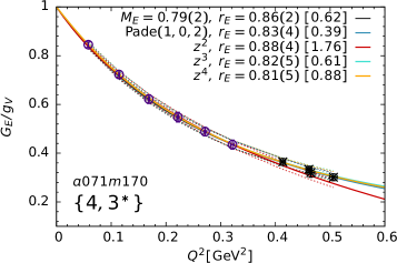
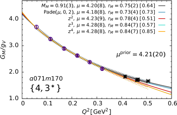
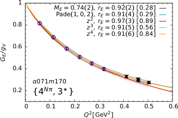
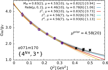
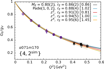
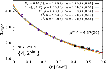
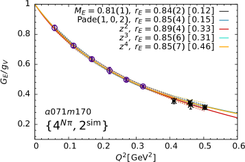
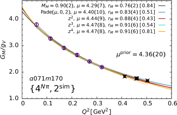
Figure 31: The data for the renormalized electric (left) and magnetic (right) form factors from the $a071m170$ ensemble fit using the dipole, $P_{2}$ Padé and $z^{2,3,4}$ ansatz. The rest is the same as in Fig. 30.

• The dipole fits to the $a071m170$ data with the $\{4^{N\pi},2^{\rm sim}\}$ strategy shown in Fig. 31 miss the low $Q^{2}$ points, and the results differ from those from the $z^{3}$ or the $P_{2}$ analyses.

In short, these CCFV fits are not yet robust. For our best estimate, we take the average of the $z^{3}$ and $P_{2}$ fits to the $\{4^{N\pi},3^{\ast}\}$ strategy data and the larger of the two analyses error. The same is done for $\mu^{u-d}\equiv\mu^{p-n}$ even though errors in it at the two values of $M_{\pi}$ are comparable and the CCFV fits are reasonable. In both cases we use half the spread between the $\{4^{N\pi},3^{\ast}\}$ and the $\{4^{N\pi},2^{\text{sim}}\}$ values as an additional systematic uncertainty for possible residual ESC and $Q^{2}$ fit ansatz dependence.

With the above selections, our final results are

$$\langle r_{E}^{2}\rangle^{u-d} = 0.85(12)(19)_{\rm sys}\ {\rm fm}^{2}\ \Rightarrow r_{E}=0.92(12)\ {\rm fm}\,\,,$$

$$\langle r_{M}^{2}\rangle^{u-d} = 0.71(19)(23)_{\rm sys}\ {\rm fm}^{2}\ \Rightarrow r_{M}=0.84(18)\ {\rm fm}\,\,,$$

$$\mu^{u-d} = 4.15(22)(10)_{\rm sys}\,.$$ (54)

These radii are consistent with values obtained from the Kelly parameterization Kelly (2004) of the experimental data given in Eq. (12) (see our review in appendix D in Ref. Jang et al. (2020b)), and the more precise value of the proton charge radius $r_{p}=0.831\pm 0.007_{\rm stat}\pm 0.012_{\rm sys}$ from the PRad experiment at Jefferson Lab Xiong et al. (2019) that claims to resolve the “proton radius puzzle” by reconciling the values from $e-p$ scattering with those from muonic hydrogen. The errors in the lattice results are, of course, much larger and do not provide independent input on the “proton radius puzzle”. The $\mu^{p-n}$ is about $2\sigma$ smaller than the precisely measured value $\mu^{p-n}|_{\rm exp}=4.7059$.

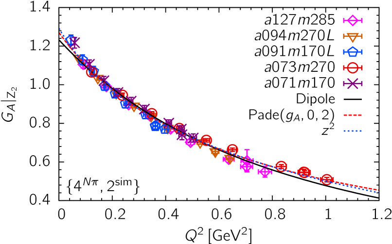
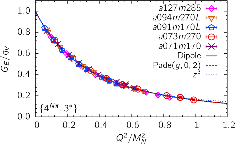
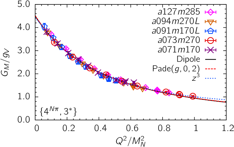
Figure 16: Comparison of the dipole, $P_{2}$ Padé, and $z$-expansion fits to the combined data from the five larger volume ensembles. We selected $\{4^{N\pi},2^{\rm sim}\}$ data for $G_{A}$ and $\{4^{N\pi},3^{\ast}\}$ for $G_{E}$ and $G_{M}$ as they show the least dependence on $a$ and $M_{\pi}$, which is neglected in these fits. Result of the $P_{2}$ fit to $G_{A}$ is given in Eq. (55), and to $G_{E}$ and $G_{M}$ in Eq. (58).

XIV Parameterizing the form factors $G_{A}$, $G_{E}$ and $G_{M}$ using Padé and $z$-expansion fits

The Padé and $z$-expansion fits to form factors presented in this section should be considered a good heuristic, i.e., they serve our primary goal to provide a good but simple parameterization of the lattice data. This is in the same spirit as the phenomenologically useful Kelly parameterization Kelly (2004) of $G_{E}$ and $G_{M}$ that are well measured in electron scattering experiments, or the rational function fit used in a recent analysis of the PRad experiment at Jefferson Lab Xiong et al. (2019). Note that the improvement in the precision with which the proton radius is extracted and the likely resolution of the “proton radius puzzle” in Ref. Xiong et al. (2019) has come from increasing the range of $Q^{2}$ and the accuracy of the data and not from the parameterization.

On the other hand, the axial form factors of the nucleon, $G_{A}$ and ${\widetilde{G}}_{P}$, that are important inputs in the analysis of neutrino-nucleus scattering are not well measured due to safety concerns with liquid hydrogen targets. Traditionally, $G_{A}$ has been parameterized using the dipole ansatz, Eq. (33), with estimates of the axial mass, $M_{A}$, ranging from 1 to 1.35 GeV, and ${\widetilde{G}}_{P}$ obtained from $G_{A}$ using the PPD hypothesis Kronfeld et al. (2019). Our analysis shows that a dipole ansatz does not have enough free parameters to fit the data over the range $0.04<Q^{2}<1$ GeV², nevertheless, we include it in this section for comparison. Furthermore, as discussed in Secs. XIII.1, XIII.2 and XIII.5, while the data for the form factors have small errors, the CCFV fits to charges and charge radii derived from them are not yet robust, a consequence of having only seven ensembles and the relatively larger errors in the $M_{\pi}\approx 170$ MeV data. Thus, we did not present a $\{a\to 0,M_{\pi}=135{\rm MeV},M_{\pi}L\to\infty\}$ limit parameterization of the form factors in those sections. On a positive note, the small dependence of $G_{A}$, $G_{E}$ and $G_{M}$ on $\{a,M_{\pi},M_{\pi}L\}$ observed in Figs. 5, 12 and 14 motivated the following heuristic analysis.

This simple parameterization assumes that the dependence on $a$, $M_{\pi}$ and $M_{\pi}L$ can be neglected, with the intent to subsequently include $a$ and $M_{\pi}$ dependent corrections as data get better. (This assumption is the least-well motivated for $G_{A}$.) To reduce the impact of the neglected finite volume corrections, we do not include data from the two small volume ensembles, $a094m270$ and $a091m170$ with $M_{\pi}L\lesssim 4$, which show some evidence of finite volume corrections. With the remaining data from five ensembles (a total of fifty $Q^{2}\neq 0$ points for $G_{A}$ and thirty for $G_{E,M}$), we compare six parameterizations for each of the three form factors: the dipole, two Padé, $P(g,0,2)$ and $P(g,1,3)$, and three $z$-expansion fits, $z^{2,3,4}$. For $G_{A}$, we use the preferred $\{4^{N\pi},2^{\rm sim}\}$ data with ${\rm Z}_{2}$ renormalization and remark that ${\rm Z}_{1}$ gives overlapping results. For $G_{E}$ and $G_{M}$, we use the $\{4^{N\pi},3^{\ast}\}$ data.

The data and three of the six fits are compared in Fig. 16. The results are summarized in Table 13. We observe the following:

• The two $P(g,0,2)$ and $P(g,1,3)$ Padé results are essentially identical and stable for all three form factors. On the basis of the Akaike criteria, $P(g,1,3)$ is an overparameterization.

• The dipole fit to $G_{A}$ is poor and shows deviations near $Q^{2}=0$ and at large $Q^{2}$. Similar, but smaller, deviations are seen for $G_{M}$. The dipole is a reasonable fit only for $G_{E}$.

• The $z^{n}$-expansion fits do not show convergence: Table 10 shows variation between the $z^{2,3,4}$ estimates, and an increase in errors. Furthermore, these estimates now depend on the choice of $t_{0}$ [see Eq. (35)] with the overall midpoint value $t_{0}=0.5~{}\text{GeV}^{2}$ giving the smallest $\chi^{2}$. As in Sec. XIII, our best choice based on the Akaike criteria is again $z^{2}$ for $G_{A}$ and $z^{3}$ for $G_{E}$ and $G_{M}$.

fit	$\langle r_{A}^{2}\rangle~{}[\text{fm}^{2}]$	$g_{A}$	$\chi^{2}/dof$	$\mathop{\langle r_{E}^{2}\rangle}\nolimits~{}[\text{fm}^{2}]$	$g_{V}$	$\chi^{2}/dof$	$\mathop{\langle r_{M}^{2}\rangle}\nolimits~{}[\text{fm}^{2}]$	$\mu$	$\chi^{2}/dof$
dipole	0.283(04)	1.232(09)	1.98 [95/48]	0.799(08)	1.003(04)	0.46 [13/28]	0.628(08)	4.499(35)	1.60 [45/28]
Padé$(g,0,2)$	0.356(13)	1.270(11)	1.27 [60/47]	0.778(19)	0.999(05)	0.42 [11/27]	0.642(23)	4.520(48)	1.64 [44/27]
Padé$(g,1,3)$	0.356(13)	1.271(11)	1.17 [53/45]	0.778(19)	0.999(05)	0.45 [11/25]	0.652(24)	4.532(48)	1.54 [38/25]
${\widehat{z}}^{2}$	0.426(15)	1.292(11)	1.15 [54/47]	1.081(16)	1.048(05)	2.25 [61/27]	0.919(24)	4.750(49)	2.42 [65/27]
${\widehat{z}}^{3}$	0.454(43)	1.301(17)	1.17 [54/46]	0.743(54)	0.996(9)	0.43 [11/26]	0.48(10)	4.424(85)	1.66 [43/26]
${\widehat{z}}^{4}$	0.67(11)	1.349(29)	1.11 [50/45]	0.66(18)	0.987(20)	0.44 [11/25]	1.04(33)	4.72(20)	1.61 [40/25]

Table 13: Results for the charge radii and charges obtained using the dipole, Padé, and $z$-expansion fits to the renormalized form factors $G_{A}(Q^{2})|_{{\rm Z}_{2}}$, $G_{E}(\frac{Q^{2}}{M_{N}^{2}})/g_{V}$ and $G_{M}(\frac{Q^{2}}{M_{N}^{2}})/g_{V}$. The fits are made to the combined data from the five larger volume ensembles. The value $t_{0}=0.5~{}\text{GeV}^{2}$ (midpoint of the $Q^{2}$ range) is used in the $z$-expansion fits for all data. The $\{4^{N\pi},2^{\text{sim}}\}$ data for $G_{A}$ and the $\{4^{N\pi},3^{*}\}$ data for $G_{E}$ and $G_{M}$ have been selected for this analysis as they exhibit the least dependence on $a$, $M_{\pi}$, and $M_{\pi}L$ as shown in Figs. 5, 12 and 14.

Incorporating these observations and bearing in mind the caveats, our best parameterizations of $G_{A}$, neglecting $\{a,M_{\pi},M_{\pi}L\}$ dependent lattice artifacts, are (i) the $\{4^{N\pi},2^{\rm sim},{\widehat{P}}_{2}\}$ fit:

$$G_{A}(Q^{2}) \equiv\frac{g_{A}}{1+b_{0}\frac{Q^{2}}{4M_{N}^{2}}+b_{1}(\frac{Q^{2}}{4M_{N}^{2}})^{2}}$$

$$=\frac{1.270(11)}{1+5.36(20)\frac{Q^{2}}{4M_{N}^{2}}-0.22(81)(\frac{Q^{2}}{4M_{N}^{2}})^{2}}\,,$$ (55)

with $\chi^{2}$/dof=1.27 and $M_{N}=939$ MeV, and (ii) the $\{4^{N\pi},2^{\rm sim},{\widehat{z}}^{2}\}$ fit that gives

$$G_{A}(Q^{2})=0.725(5)-1.63(3)z+0.17(13)z^{2}\,,$$ (56)

with $\chi^{2}$/dof=1.15, and $z$ defined in Eq. (35) with $t_{0}=0.5$ GeV². For our best results, we take the average of these $\{4^{N\pi},2^{\rm sim},{\widehat{P}}_{2}\}$ and $\{4^{N\pi},2^{\rm sim},{\widehat{z}}^{2}\}$ values given in Table 13 to get

$$g_{A}^{u-d} = 1.281(11)(22)_{\rm sys}\,,$$

$$\langle r_{A}^{2}\rangle^{u-d} = 0.391(15)(70)_{\rm sys}\ {\rm fm}^{2}\ \,,$$ (57)

which are slightly smaller than the values in Eqs. (42) and (45). The second, systematic, error is taken to be the difference between the two estimates averaged.

Similarly, the results of the $\{4^{N\pi},3^{\ast},{\widehat{P}}_{2}\}$ and $\{4^{N\pi},3^{\ast},{\widehat{z}}^{3}\}$ fits to $G_{E}$ and $G_{M}$ are

$$G_{E}(Q^{2}) =\frac{0.999(5)}{1+11.72(29)\frac{Q^{2}}{4M_{N}^{2}}+38.5(1.9)(\frac{Q^{2}}{4M_{N}^{2}})^{2}}\,,{\rm or}$$

$$=0.290(3)-1.23(3)z+1.72(19)z^{2}$$

$$\qquad\qquad\qquad\qquad\qquad\qquad{}+2.48(35)z^{3}\,,$$

$$G_{M}(Q^{2}) =\frac{4.52(5)}{1+9.68(35)\frac{Q^{2}}{4M_{N}^{2}}+21.3(1.8)(\frac{Q^{2}}{4M_{N}^{2}})^{2}}\,,{\rm or}$$

$$=1.613(11)-5.74(14)z+6.1(1.2)z^{2}$$

$$\qquad\qquad\qquad\qquad\qquad\qquad{}+11.9(2.5)z^{3}\,.$$ (58)

Both sets of fits have very similar $\chi^{2}$/dof: $\approx 0.43$ and $\approx 1.65$ for $G_{E}$ and $G_{M}$, respectively. The variance-covariance matrices of the above six fits are given in Appendix I. The results are:

$$\{4^{N\pi},3^{\ast},{\widehat{P}}_{2}\}$$

fm²

fm²

 .

(59)

The second, systematic, error in both cases is taken to be half the spread between the $\{4^{N\pi},3^{\ast},{\widehat{P}}_{2}\}$, $\{4^{N\pi},3^{\ast},{\widehat{z}}^{3}\}$, $\{4^{N\pi},2^{\rm sim},{\widehat{P}}_{2}\}$ and $\{4^{N\pi},2^{\rm sim},{\widehat{z}}^{3}\}$ estimates.

Next, we explored adding corrections due to $\{a,M_{\pi}\}$ in these combined fits by expanding all parameters in them, for example $b_{0}\to(b_{0}^{0}+b_{0}^{a}a+b_{0}^{m}{\cal O}(M_{\pi}^{2}))$, where ${\cal O}(M_{\pi}^{2}))$ is $\log(M_{\pi}^{2})$ for $\mathop{\langle r_{E}^{2}\rangle}\nolimits$ and $1/M_{\pi}$ for $\mathop{\langle r_{M}^{2}\rangle}\nolimits$. The result is that the $\chi^{2}$ is reduced only marginally but the errors in the observables jump by a factor of 6 or more with any (even one) additional parameter. Also, in most cases the extra parameter(s) are essentially undetermined indicating overparameterization. Our conclusion again is that much higher precision data on more ensembles are needed to include $\{a,M_{\pi}\}$ dependent corrections in this approach.

Another estimate of $\mu^{u-d}$ is obtained from a linear fit to the $G_{M}/G_{E}$ data as shown in Fig. 15. The left panel shows separate fits to the $a091m170L$ and $a071m170$ data with the $\{4^{N\pi},3^{\ast}\}$ strategy. The right panel shows the fit to the combined data from these two ensembles. (Data from the other three larger volume $M_{\pi}\sim 270$ MeV ensembles are included only for comparison.) The result from the fit to the two $M_{\pi}\approx 170$ MeV ensembles, $\mu^{u-d}=4.67(12)$, is consistent with that in Eq. (59).

This heuristic analysis has the advantage of evading the two-step process used to get results given in Sec. XIII: first a parameterization of the $Q^{2}$ behavior and then CCFV fits to the observables with just leading order corrections in $\{a,M_{\pi},M_{\pi}L\}$. The disadvantage is assuming that the $\{a,M_{\pi},M_{\pi}L\}$ corrections can be neglected, even though the data in Figs. 5, 12 and 14 suggest it. The remarkable outcome is that the estimates from the heuristic analysis are consistent with those given in Eqs. (42), (45), and (54) but with much smaller errors in all cases. Also note that these fits give $G_{E}(Q^{2}=0)=0.999(5)$ and $G_{M}(Q^{2}=0)=4.52(5)$, i.e., a necessary consistency check against the precisely known values for the electric charge and the magnetic moment.

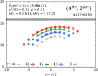
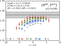
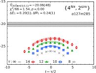
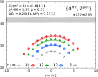
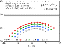
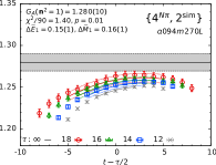
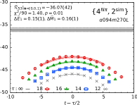
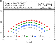
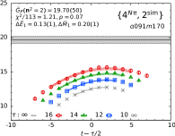
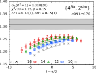
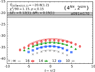
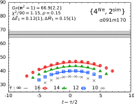
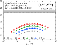
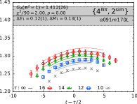
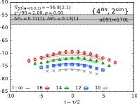
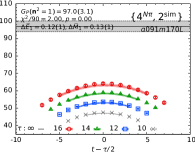
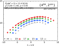
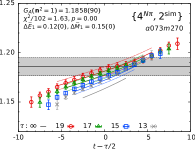
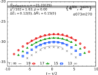
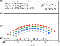
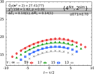
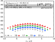
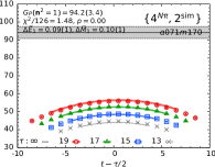
Figure 24: Matrix elements of the axial and pseudoscalar currents that give (i) ${\widetilde{G}}_{P}$ (from $R_{51}$ with ${\bm{n}}^{2}=2$ defined in Eq. (20)] in column one, (ii) $G_{A}$ (from $R_{53}$ with ${\bm{n}}^{2}=1$ and $q_{z}=0$ defined in Eq. (22)] in the second column, (iii) the combination $\frac{{\widetilde{G}}_{P}}{2M_{N}}-\frac{(M+E)}{q_{3}^{2}}G_{A}$ [from $R_{53}$ with $q_{3}=(0,0,1)2\pi/La$] in the third column, and (iv) $G_{P}$ (from $R_{5}$ defined in Eq. (24)) in the right column. All data are with the $\{4^{N\pi},2^{\rm sim}\}$ strategy and plotted versus the shifted operator insertion time $t-\tau/2$. The rest is the same as in Fig. 23.

To understand why the dipole fit does not work for $G_{A}$ in this case also, we note that the errors on points at small $Q^{2}$ grow as $Q^{2}\to 0$ because the extrapolation in $\tau$ to remove ESC in the $\{4^{N\pi},2^{\rm sim}\}$ fits is large on the $170$ MeV ensembles as can be seen from Fig. 24. Similarly, the errors grow as $Q^{2}$ increases because the statistical signal-to-noise degrades. Thus, the dipole fit in Fig. 16 with $g_{A}$ and $M_{A}$ left as free parameters is anchored by the smaller error points in the middle and fails at both ends as it does not have enough degrees of freedom to fully capture the curvature. The Padé $\{g_{A},0,2\}$, with one additional degree of freedom, is sufficient.

Collab. Ref. $g_{A}^{u-d}$ $g_{S}^{u-d}$ $g_{T}^{u-d}$ $\langle r_{A}^{2}\rangle^{u-d}$ $g_{P}^{\ast}$ $g_{\pi NN}$ $\mathop{\langle r_{E}^{2}\rangle}\nolimits^{u-d}$ $\mathop{\langle r_{M}^{2}\rangle}\nolimits^{u-d}$ $\mu^{p-n}$ Action [fm²] [fm²] [fm²] NME This $1.32(6)$ $1.06(9)$ $0.97(3)$ 0.428(53) 7.9(7) 12.4(1.2) 0.85(12) 0.71(19) 4.15(22) $N_{f}=2+1$ Work A $(4)_{\rm ES}(2)_{Z}(2)_{a}(2)_{\rm FV}$ $(2)_{Z}(6)_{a}$ $(1)_{\rm ES}(1)_{Z}(1)_{a}$ $(30)_{\rm ES}$ $(9)_{\chi}$ $(19)_{\rm ES}$ $(23)_{\rm ES}$ $(10)_{\rm ES}$ clover-on-clover NME This $1.270(11)$ 0.356(13) 0.778(19) 0.642(23) 4.52(5) $N_{f}=2+1$ Work B $(22)_{\rm sys}$ $(70)_{\rm sys}$ $(50)_{\rm sys}$ $(80)_{\rm sys}$ $(10)_{\rm sys}$ clover-on-clover PNDME Gupta et al. (2018, 2017); Jang et al. (2020b, a) $1.218(25)(30)$ $1.022(80)(60)$ $0.989(32)(10)$ 0.24(7) 0.591(62) 0.45(12) 3.94(16) $N_{f}=2+1+1$ 0.24(3) 0.586(21) 0.495(50) 3.98(15) Clover-on-HISQ ETMC Alexandrou et al. (2021, 2020, 2019) $1.286(23)$ $1.35(17)$ $0.936(25)(16)$ 0.343(42) 0.634(26) 0.51(13) 3.97(16) $N_{f}=2+1+1$ Twisted Mass RBC- Abramczyk et al. (2020) $1.15(5)$ $0.9(3)$ $1.04(5)$ $N_{f}=2+1$ UKQCD Domain Wall CalLat Walker-Loud et al. (2020); Chang et al. (2018) $1.2642(93)$ $N_{f}=2+1+1$ DW-on-HISQ PACS Ishikawa et al. (2018); Shintani et al. (2019); Tsukamoto et al. (2020) $1.273(24)$ 0.419(28) 0.766(26) 0.648(58) 4.42(14) $N_{f}=2+1$ $(9)_{Z}(5)_{\rm ES}$ $(49)_{\rm sys}$ $(49)_{\rm ES}$ $(441)_{\rm ES}$ $(32)_{\rm ES}$ clover-on-clover JLQCD Ishikawa et al. (2018) 1.123(28) 0.88(8) 1.08(3) Overlap $(29)_{\chi}(90)_{a}$ $(3)_{\chi}(7)_{a}$ $(3)_{\chi}(9)_{a}$ RQCD Bali et al. (2020) $1.302(45)$ 0.449(88) 8.68(45) 14.78(1.81) $N_{f}=2+1$ ($!z^{4+3}$) $(42)_{\rm ES}(38)_{m}(46)_{a}$ $(42)_{\rm ES}(42)_{m}(49)_{a}$ $(18)_{\rm ES}(23)_{m}(16)_{a}$ $(72)_{\rm ES}(98)_{m}(67)_{a}$ 1.229(24) 0.272(33) 8.30(24) 12.93(80) clover-on-clover (dipole) $(6)_{\rm ES}(3)_{m}(17)_{a}$ $(6)_{\rm ES}(7)_{m}(24)_{a}$ $(14)_{\rm ES}(6)_{m}(8)_{a}$ $(44)_{\rm ES}(20)_{m}(44)_{a}$ Mainz Harris et al. (2019); Djukanovic et al. (2021) $1.242(25)_{\rm stat}$ $1.13(11)_{\rm stat}$ $0.965(38)_{\rm stat}$ 0.800(25) 0.661(30) 4.71(11) $N_{f}=2+1$ $(+00,-31)_{\rm sys}$ $(+07,-06)_{\rm sys}$ $(+13,-41)_{\rm sys}$ $(22)_{\rm sys}$ $(11)_{\rm sys}$ $(13)_{\rm sys}$ clover-on-clover LHPC Hasan et al. (2019, 2018) $1.265(49)$ 0.927(303) 0.972(41) 0.249(12) 0.608(15) 3.899(38) $N_{f}=2+1$ 0.295(68) 0.787(87) 4.75(15) clover-on-clover $\chi$QCD Liang et al. (2018) $1.254(16)(30)$ $N_{f}=2+1$ Overlap-on-DW

Table 14: Comparison of lattice QCD results from simulations with $N_{f}=2+1+1$ and $2+1$ flavors that satisfy the criteria on chiral and continuum extrapolation defined in the text. Only the latest (best) results for each quantity from a given collaboration/calculation are quoted. We present our (NME) results from two sets of analyses: (A) the analysis presented in Sec. XIII, and (B) in Sec. XIV. The PNDME estimates on the top are from a $z^{3,4}$ analysis and at the bottom from a dipole fit. The two RQCD Bali et al. (2020) results are from the $z$-expansion (top) and the dipole (below) fits to the $Q^{2}$ behavior of $G_{A}$. The notation for systematic errors is: FV=finite volume, Z=renormalization, ES=excited states, $a$=discretization, $\chi$=$m$=chiral, and sys=systematic (or when the second error has no label)

XV Comparison with Previous Lattice QCD Calculations

In this section, we compare with results from other recent lattice calculations done with either 2+1+1 or 2+1 dynamical flavors. We assume that a dynamical charm in the lattice generation does not significantly impact the quantities composed of light quarks that are investigated here; i.e., the two formulations give the same results. For a more extensive review of the calculation of the charges, we direct the reader to the Flavor Lattice Averaging Group (FLAG) Reviews 2019 Aoki et al. (2020) and 2021 Aoki et al. (2021).

It is important to note that all of these isovector quantities from different calculations are expected to only agree at the physical point, and thus a CCFV extrapolation is necessary. We have therefore applied the following criteria in selecting the calculations to compare. We require that (i) the results are either obtained at $M_{\pi}\approx 135$ MeV or have been extrapolated to it, and similarly (ii) they include ensembles with $a<0.1$ fm or a continuum extrapolation has been performed. (iii) We find that so far no other calculation has carried out the extensive high statistics analysis of excited states presented in this work, so we do not apply an excited-state criterion for inclusion, but will comment on the method used to control ESC and the outcome.

The results compared are summarized in Table 14. For each collaboration, we quote the latest (or best in the words of the authors) value for each observable, which is often given in different publications. Overall, it is evident that a complete control over systematic uncertainties, especially excited-state effects, is still work under progress.

The PNDME results Gupta et al. (2018, 2017); Jang et al. (2020b) are from a clover-on-HISQ formulation using eleven 2+1+1-flavor HISQ ensembles, including two at the physical pion mass. All the quoted results are from CCFV fits to data with the $\{4,3^{\ast}\}$ strategy, i.e., they represent the status Aoki et al. (2020) before $N\pi$ (or $N\pi\pi$) states were included in fits to remove the ESC.

The ETM Collaboration Alexandrou et al. (2021, 2020, 2019) has presented results for most of the quantities analyzed in this work. Their latest results are from one 2+1+1-flavor twisted mass clover-improved ensemble with $a=0.0801(4)$ fm, $M_{\pi}=139(1)$ MeV, $M_{\pi}L=3.62$, so issues of continuum extrapolation, finite volume corrections and chiral behavior are not addressed. (Our $a071m170$ ensemble provides data at similar values of $Q^{2}$.) Their statistical sample is 750 lattices separated by 4 trajectories each, and results for the isovector charges Alexandrou et al. (2020) are taken from a two-state fit, $\{2,2\}$ in our notation. Their axial form factors Alexandrou et al. (2021) do not satisfy the PCAC relation, and their estimates presented for ${\widetilde{G}}_{P}$ and $G_{P}$ are not the calculated values but those obtained from $G_{A}$ using the pion-pole dominance relation. Consequently, we do not quote their estimates for $g_{P}^{\ast}$ and $g_{\pi NN}$. Both the dipole and $z$-expansion fits to $G_{A}(Q^{2})$ obtained from $\{2,2\}$ strategy work well and give $\langle r_{A}^{2}\rangle=0.343(42)(16)$ fm², which is consistent with our $\{4,3^{\ast}\}$ value. The electric and magnetic form factors, presented in Ref. Alexandrou et al. (2019), are well fit by a dipole ansatz, however, they differ from the Kelly parameterization at small $Q^{2}$, as also seen in the PNDME results in Ref. Jang et al. (2020b).

The RBC-UKQCD Collaboration has analyzed two ensembles of 2+1-flavor domain wall (DW) fermions with Iwasaki plus dislocation-suppressing-determinant-ratio (DSDR) gauge action at $a=1.378(7)$ fm and with $M_{\pi}=249.4(3)$ and $172.3(3)$ MeV. They report issues of long autocorrelations in a statistical sample of only 700 trajectories, which may explain an underestimate of $g_{A}$ and a large uncertainty in $g_{S}$.

The CalLat Collaboration Walker-Loud et al. (2020); Chang et al. (2018) report $g_{A}^{u-d}$ with percent level accuracy using the domain-wall-on-HISQ formulation. In their calculation, the operator is already summed over all insertion times $t$ during generation; therefore, they can only analyze their data versus $\tau$. They use two-state fits to data starting at much smaller source-sink separations, $0.2\lesssim\tau\lesssim 0.8$ fm, where many higher excited states contribute and sensitivity to contributions from $N\pi$ states would be small. They do not explicitly include an $N\pi$ state in their analysis. Thus, the balance between control over statistical versus systematic errors, especially the impact of the inclusion of the $N\pi$ state(s), remains to be addressed. The CCFV fits are made to data from 16 ensembles at three values of $a\approx 0.09,\ 0.12,0.15$ fm and five values of $M_{\pi}\approx 400,350,310,220,130$ MeV.

The PACS Collaboration Ishikawa et al. (2018); Shintani et al. (2019); Tsukamoto et al. (2020) uses a single $128^{4}$ ensemble generated with 2+1-flavor stout-smeared $O(a)$ improved Wilson-clover fermions and Iwasaki gauge action at $a=0.0846(7)$ fm and $M_{\pi}=135(9)$ MeV. While the lattice volume is large, $M_{\pi}L=7.4$, results have been presented from only 20 lattices, each separated by 10 trajectories. The JLQCD Yamanaka et al. (2018) use 2+1-flavor overlap formulations with a single value of $a=0.11$ fm, 4 values of $M_{\pi}=293,379,453,540$ MeV and 50 gauge configurations. In both calculations, even though some of their estimates are reasonable, the control over the statistical and various systematic uncertainties we have discussed is limited. For example, on the key issue of excited states, in Ref. Shintani et al. (2019) they find no significant excited-state effects over the range $0.84<\tau<1.35$ fm, in contradiction to all other calculations. Also, estimates from $96^{4}$ Ishikawa et al. (2018) and $128^{4}$ Shintani et al. (2019) lattices with the same lattice spacing but with $M_{\pi}=146$ versus $135$ MeV show much larger differences than expected, presumably due to low statistics in both calculations.

The RQCD Collaboration Bali et al. (2020) has presented results for the axial form factors on 37 ensembles with 2+1 flavors of nonperturbatively $O(a)$ improved Wilson-clover fermions with a tree- level Symanzik improved gauge action generated by the CLS Collaboration Bruno et al. (2015). These ensembles cover five values of the lattice spacing and include two physical pion mass ensembles. To remove excited states they use a strategy similar to $\{3,2\}$ for the axial charge and $G_{A}$, and to $\{4^{N\pi},3^{\ast}\}$ for ${\widetilde{G}}_{P}$ and $G_{P}$ form factors. The resulting form factors satisfy the PCAC relation at a level similar to that presented in this work. They find that both the dipole and the $z$-expansion ansatz fit the $Q^{2}$ behavior of $G_{A}(Q^{2})$; however, results for $g_{A}^{u-d}$, $\langle r_{A}^{2}\rangle^{u-d}$, and $g_{P}^{\ast}$ are different as can be seen from the summary in Table 14.

The Mainz Collaboration Harris et al. (2019) analyzed 11 CLS ensembles Bruno et al. (2015) that are common with the RQCD work described above. On these ensembles, the pion mass ranges between $203$ and $353$ MeV. To control ESC they explore the summation method and two-state fits with a common value for $\Delta M_{1}$ for six quantities, the three charges and three Mellin moments that give the momentum fraction, helicity, and transversity. Note that our data for $\Delta M_{1}$ (or $\Delta{\widetilde{M}}_{1}$) for the three charges given in Table 2 and for the three moments given in Ref. Mondal et al. (2020) do not support using a common value for $\Delta M_{1}$ in the analysis of all six quantities. Their final results are also obtained with the CCFV ansatz given in Eq. (41), which they call ABDE. For the vector form factors Djukanovic et al. (2021), they analyze 10 CLS ensembles including one with the physical pion mass; however, errors in data from it are large. The ESC is controlled using the summation and two-state fit methods ($\{2,2\}$ in our notation), which give consistent values. The errors in the data with the summation method, especially at the larger $Q^{2}$, are much larger. They employ dipole and $z$-expansion parameterization of the $Q^{2}$ behavior, and the chiral-continuum extrapolation using heavy baryon chiral perturbation theory (HBChPT) supplemented with leading order corrections for lattice discretization and finite volume. Their final estimates are obtained from a model-agnostic average (summation, two-state fits, dipole, $z$-expansion, HBChPT, and cuts on $Q^{2}$ and $M_{\pi}^{2}$ values) with weights given by the Akaike information criteria.

The LHPC Collaboration Hasan et al. (2019, 2018) analyzed two physical pion mass 2+1-flavor ensembles generated with 2-HEX-smeared Wilson-clover action (the Budapest-Marseille-Wuppertal ensembles). One of their main observations from the study of charges Hasan et al. (2019) is a significant variation in $Z_{S}$ between the RI^′-MOM and RI-sMOM renormalization schemes which, along with the statistical errors and extrapolation in $a$ uncertainty, accounts for the large error in $g_{S}$. In Ref. Hasan et al. (2018), they present results for $\mu^{p-n}$ and charge radii from two methods: traditional ($z$-expansion) and derivative. In Table 14, we quote their results from the traditional method as recommended by them, and from the two analyses for handling ESC: $\tau/a=10$ ratio data (top) and summation (bottom), which differ. Systematic uncertainties were not evaluated in either set of estimates.

The $\chi$QCD Collaboration Liang et al. (2018) used the overlap-on-domain-wall formulation on three 2+1-flavor domain-wall ensembles generated by the RBC/UKQCD Collaboration. On each of these ensembles, data with 5–6 values of the valence pion mass are generated. They obtain $g_{A}^{u-d}$ using a CC fit to these partially quenched data.

From the summary of results in Table 14, we conclude that, overall, results for $g_{T}^{u-d}$ are consistent within $5\%$, and for $g_{S}^{u-d}$ within $10\%$, and sensitivity to excited states in their extraction is small. For all other quantities such as $g_{A}^{u-d}$, the charge radii, $g_{P}^{\ast}$ and $g_{\pi NN}$, results from analyses that do not include the $N\pi$ states give smaller values compared to phenomenology.

XVI Conclusions

We have presented an analysis of isovector charges and axial and electromagnetic form factors on seven 2+1-flavor Wilson-clover ensembles generated by the JLab/W&M/LANL/MIT Collaborations Edwards et al. (2016) and described in Table 15. This unitary clover-on-clover calculation is an improvement over our previous work using the nonunitary clover-on-HISQ formulation Gupta et al. (2018, 2017); Jang et al. (2020a, b). In addition, high-statistics data have allowed us to make significant progress in understanding key issues in controlling other systematic uncertainties including excited state contamination in various nucleon matrix elements.

The excited-state contributions to each observable are analyzed using a number of possible values of the energy of the first excited state, which is assumed to provide the dominant contamination. The axial form factors extracted including the low-lying multihadron $N\pi$ state satisfy the PCAC relation between them and are consistent with the pion-pole dominance hypothesis. We also find evidence that the $N\pi\pi$ state, theoretically supported by the vector-meson dominance hypothesis, contributes to the electric and magnetic form factors. They show much less sensitivity to the excited state mass gap, and the results agree with the experimental data parameterized using the Kelly result Kelly (2004).

Results of the pseudoscalar decay constant, $F_{\pi}$, after CCFV fits to data with two methods for renormalization are $F_{\pi}|_{{\rm Z}_{1}}=93.0(3.9)$ (this CCFV fit is shown in Fig. 36) and $F_{\pi}|_{{\rm Z}_{2}}=95.9(3.5)$. These estimates agree with the experimental value to within a few percent. Noting that $F_{\pi}$ data points have small statistical errors, the difference and the size of the errors after CCFV fits, $\approx 4\%$, should be regarded as a measure of the overall accuracy of the CCFV fits with seven data points, especially in observables that show significant variations with respect to $\{a,M_{\pi},M_{\pi}L\}$.

The results for the three isovector charges obtained from the forward matrix elements [see Eq. (43)] are $g_{A}^{u-d}=1.32(6)(5)_{\rm sys}$ (this estimate includes input from the extrapolation of the $Q^{2}\neq 0$ data), $g_{S}^{u-d}=1.06(9)(6)_{\rm sys}$, and $g_{T}^{u-d}=0.97(3)(2)_{\rm sys}$. The first overall analysis error is conservative with respect to the variation observed under CCFV extrapolations. Estimation of systematic uncertainties are discussed in Sec. XIII.1. The scalar and tensor charges $g_{S,T}^{u-d}$ do not show a significant dependence on the value of the first excited state mass, so we consider their estimate robust.

The value of $g_{A}^{u-d}$ has been extracted in two ways, one from the forward matrix element and the second from an extrapolation of the axial form factor to $Q^{2}=0$. These two ways must give the same result in the continuum limit that should agree with the experimental value. We find that $g_{A}^{u-d}$ is sensitive to the inclusion of the $N\pi$ state. Our results have a $\sim 10\%$ spread depending on the ESC strategy and the $Q^{2}$ fits used as discussed in Sec. XIII.1. A snapshot of the spread is given in Table 10. The change in $G_{A}(Q^{2})$ on including the $N\pi$ state is, in most cases, a few percent (see Table 18): the largest change ($3$–$5$%) is in the smallest $Q^{2}$ point (${\bm{n}}^{2}=1$) on the $M_{\pi}\approx 170$ MeV ensembles, however, it is precisely the change in the low $Q^{2}$ points that has the largest impact on the extraction of $g_{A}^{u-d}$ from fits to $G_{A}$. Similarly, the change in the forward matrix element is about $6\%$ (see Fig. 3). These changes are of the same size as our overall analysis error estimate, $\sim 5\%$, and the additional systematic uncertainty included in the final result $g_{A}^{u-d}=1.32(06)(05)_{\rm sys}$. Thus, this level of the possible contribution of the $N\pi$ state in extracting $G_{A}$, and its impact on the improvement of the PCAC relation, is just at the level of our current resolution. Our conclusion, therefore, is as follows: to fully resolve the issue of the size of the contributions of the $N\pi$ states in the extraction of $G_{A}$ and to improve the precision of lattice estimates of $g_{A}^{u-d}$ requires more extensive data.

To fit the $Q^{2}$ dependence of the form factors, we explore the $z$-expansion, the dipole ansatz, and Padé fits. Estimates from the $z^{2,3,4}$ truncation of the $z$-expansion give consistent results for the axial form factors and we take final values from the $z^{2}$ fits to avoid overparameterization. For the vector form factors we use the $z^{3}$ truncation. The second order Padé, $P(g,0,2)$, with three free parameters, is found to provide an equally good parameterization. The dipole ansatz does not provide a good fit to $G_{A}(Q^{2})$ obtained including the $N\pi$ state when removing the ESC. It provides a reasonable fit to the electric form factor, and less so to the magnetic.

We have carried out two analyses to get charge radii from the form factors, and both sets of results are summarized in Table 14. In the first, the $Q^{2}$ dependence of data from each ensemble is parameterized using the dipole, Padé and $z$-expansion, and the lattice artifacts in the resulting values of the charges and the charge radii due to discretization, finite volume effects, and heavier than physical values of quark masses are then removed by simultaneous CCFV fits keeping leading order corrections in the three variables $\{a,M_{\pi},M_{\pi}L\}$. The results are the following: (i) the axial charge radius squared, $\langle r_{A}^{2}\rangle=0.428(53)(30)_{\rm sys}$ fm², (ii) the induced pseudoscalar charge, $g_{P}^{\ast}=7.9(7)(9)_{\rm sys}$, (iii) the pion-nucleon coupling $\mathop{g_{\pi{NN}}}\nolimits=12.4(1.2)$, (iv) the electric charge radius squared, $\langle r_{E}^{2}\rangle^{u-d}=0.85(12)(19)_{\rm sys}\ {\rm fm}^{2}$, (v) the magnetic charge radius squared, $\langle r_{M}^{2}\rangle^{u-d}=0.71(19)(23)_{\rm sys}\ {\rm fm}^{2}$, and (vi) the magnetic moment $\mu^{u-d}=4.15(22)(10)_{\rm sys}$. At this point, we do not consider deviations from phenomenological/experimental results significant. In the axial channel, to obtain this improved consistency of results and for the form factors to satisfy the PCAC relation between them, it was crucial to include the $N\pi$ state in the removal of ESC.

The electric and magnetic form factors $G_{E}$ and $G_{M}$, shown in Figs. 12 and 14, exhibit much less sensitivity to the value of the mass gap of the excited state. Our results agree with the Kelly parameterization of the experimental data over the range $0.04\lesssim Q^{2}\lesssim 1.2$ GeV² when plotted as a function of $Q^{2}/M_{N}^{2}$, and show no significant variation with respect to either $a$ or $M_{\pi}^{2}$. This agreement is a major improvement over our previous work using the clover-on-HISQ formulation presented in Ref. Jang et al. (2020b).

A second, heuristic, analysis of form factors, presented in Sec. XIV, explores the same set of parameterizations (see Table 13) but makes a single fit to data from all five larger volume ensembles as shown in Figs. 5, 12 and 14, i.e., ignoring $\{a,M_{\pi},M_{\pi}L\}$ dependent artifacts. The $P(g,0,2)$ Padé does a good job of parameterizing the $Q^{2}$ behavior and the results are given in Eqs. (55) and (58).

The results for $g_{A}^{u-d}$, $\langle r_{A}^{2}\rangle^{u-d}$, $\mathop{\langle r_{E}^{2}\rangle}\nolimits^{u-d}$, $\mathop{\langle r_{M}^{2}\rangle}\nolimits^{u-d}$, and $\mu^{u-d}$ from these two sets of analyses, summarized in Table 14, are consistent but the errors from the second set are smaller; a consequence of the analysis becoming simpler on ignoring $\{a,M_{\pi},M_{\pi}L\}$ dependent artifacts.

Our goal is to provide a parameterization of the form factors themselves versus $Q^{2}$ for input into phenomenological analyses. In the analysis method “A,” we do not have a robust theoretical guide or adequate data for performing CCFV extrapolations of each of the coefficients of the $z$-expansion or Padé fits (the $a_{k}$ in Eq. (34) or the $b_{i}$ in Eq. (36)) determined from fits to individual ensembles. In method “B,” we make the assumption that the $\{a,M_{\pi},M_{\pi}L\}$ dependent artifacts can be ignored (see the data in Fig. 16). Under this assumption, Eqs. (55), (56), and (58) give our continuum limit parameterization of the form factors.

Overall, our results for the form factors are consistent with phenomenological/experimental values. For this agreement, it was essential to include the low-energy $N\pi$ ($N\pi\pi$) excited state in the analysis of the axial form factors, and to a smaller extent in the vector channel. Motivation for including these states comes from $\chi$PT, pion-pole dominance for axial, and vector meson dominance for vector channels. Our data support these hypotheses, and the estimates of $\Delta M_{1}$ are in rough agreement with those expected with $N\pi$ (or $N\pi\pi$ for vector) states (see Figs. 22 and 10 for the axial and vector cases, respectively). The change in the axial form factors is only a few percent; however, it is large, $\sim 35\%$, in both the induced pseudoscalar, ${\widetilde{G}}_{P}$, and the pseudoscalar, $G_{P}$, form factors. With these changes, the resulting form factors satisfy the PCAC relation between them. Furthermore, the estimates of the induced pseudoscalar charge, $g_{P}^{\ast}=7.9(7)(9)$, and of the pion-nucleon coupling $\mathop{g_{\pi{NN}}}\nolimits=12.4(1.2)$ become consistent with phenomenology.

The change in the electric and magnetic form factors between the four ESC strategies is small as shown in Figs. 12 and 14. A significant reduction in the dependence on $\{a,M_{\pi}\}$ of both form factors is observed when plotted versus $Q^{2}/M_{N}^{2}$. This provided motivation for the Padé and $z$-expansion parameterization presented in Sec. XIV and the results in Eqs. (55)–(59).

To increase precision, address the issue of the spread in results due to different estimates of the relevant mass gap, and to resolve whether additional $N\pi$ state[s] should be included in the analysis, higher statistics data at more values of $\{a,M_{\pi},M_{\pi}L\}$ are needed. The benchmarks for improvement will continue to be satisfying the PCAC relation between the axial form factors, the agreement with the experimental value $g_{A}^{u-d}=1.2764(1)$, and the well measured vector form factors $G_{E}$ and $G_{M}$.

Appendix A Glossary of labels used to describe the various fits made

A summary of the abbreviations used to describe the various analysis strategies and fits is given below in order of the three entries such as in $\{4^{N\pi},3^{\ast},{\widehat{P}}_{2}\}$.

The first entry specifies the fits to the two-point function used to extract the spectrum. It has two possibilities:

• $\{4\}$ denotes that four-state fits are made to the two-point function. Empirical Bayesian priors with wide widths for excited state energies and amplitudes are used only to stabilize the fits. These fits are illustrated in the left-hand column in Fig. 1.

• $\{4^{N\pi}\}$ denotes that a prior for $\Delta E_{1}$ with a narrow width centered about the energy of the noninteracting $N\pi$ (or of $N\pi\pi$ that is essentially degenerate) state is used in four-state fits to the two-point function. Priors on higher states are similar to those in $\{4\}$ fits. These fits are illustrated in the right-hand column in Fig. 1.

The second entry specifies the four different fits made to the three-point functions:

• $\{3^{\ast}\}$ specifies that three-state fits are made to the three-point functions with the spectrum taken from either $\{4\}$ or $\{4^{N\pi}\}$ fits to two-point functions, and the $\langle 2|O|2\rangle$ term in Eq. (18) is set to zero.

• $\{2^{A_{4}}\}$: This is a two-state fit to the three spatial axial vector and the pseudoscalar three-point functions with a common $\Delta E_{1}$ determined from fits to the $A_{4}$ correlator. The ground state parameters are taken from either $\{4\}$ or $\{4^{N\pi}\}$ fits.

• $\{2^{\rm sim}\}$: This is a two-state fit to a set of three-point functions. In the axial channel it denotes that a simultaneous fit to the four axial vector and the pseudoscalar channels is made with a common $\Delta E_{1}$. In the vector channel it denotes a simultaneous fit to the three distinct correlation functions described in Sec. XII. The ground state parameters are taken from either $\{4\}$ or $\{4^{N\pi}\}$ fits. In both cases, the output mass gap is called $\Delta{\widetilde{E}}_{1}$.

• $\{2^{\rm free}\}$: This is a two-state fit to an individual three-point function with $\Delta E_{1}$ left as a free parameter. The output mass gap is called $\Delta{\widetilde{E}}_{1}$. The ground state parameters are taken from either $\{4\}$ or $\{4^{N\pi}\}$ fits.

The third entry specifies the six different fits made to the form factors to parameterize the $Q^{2}$ behavior:

• $\{D\}$ and $\{\widehat{D}\}$: “D” stands for a dipole fit. The hat in $\{\widehat{D}\}$ specifies that subsequent CCFV fits to quantities such as $g_{A}$, $\mathop{\langle r_{E}^{2}\rangle}\nolimits$, $\mathop{\langle r_{M}^{2}\rangle}\nolimits$ and $\mu$ have been carried out neglecting the two small volume points, $a094m270$ and $a091m170$, and the finite-volume correction term have been neglected, i.e., only a CC fit is performed.

• $\{z^{k}\}$ and $\{{\widehat{z}}^{k}\}$: These are z-expansion fits truncated at power $k$. The hat in the label $\{\widehat{z}\}$ again specifies that subsequent CC fits have been done neglecting the two small volume points, $a094m270$ and $a091m170$, and the finite-volume correction term have been neglected, i.e., only a CC fit is performed.

• $\{P_{n}\}$ and $\{{\widehat{P}}_{n}\}$: “P” stands for a Padé fit. The subscript $n$ specifies the order of the Padé as discussed in Sec. X. The hat in $\{\widehat{P}\}$ again specifies that the two small volume points, $a094m270$ and $a091m170$, and the finite-volume correction term have been neglected, i.e., only a CC fit is performed.

Appendix B Lattice parameters and the values of $Q^{2}$ from the two four-state fits, $\{4\}$ and $\{4^{N\pi}\}$

In this appendix, we give the parameters of the seven ensembles in Table 15 and the corresponding parameters used in the calculation of the clover propagators in Table 16. The values of momentum transfer squared, $Q^{2}$, obtained from the two four-state fits, $\{4\}$ and $\{4^{N\pi}\}$, to the two-point correlation function are given in Table 17.

ID	$\beta$	$a$	$M_{\pi}$	$M_{N}^{\{4\}}$	$M_{N}^{\{4^{N\pi}\}}$	Size		$M_{\pi}L$	Lattices	$N_{\rm HP}$	$N_{\rm LP}$	$\tau$
		[fm]	[MeV]	[MeV]	[MeV]	$L/a$	$T/a$
$a127m285$	6.1	0.127(2)	285(5)	961(15)	958(15)	32	96	5.87	2,002	8,008	256,256	{8,10,12,14}
$a094m270$	6.3	0.094(1)	269(3)	982(15)	986(11)	32	64	4.09	2,469	7,407	237,024	{8,10,12,14,16}
$a094m270L$	6.3	0.094(1)	269(3)	979(11)	976(11)	48	128	6.15	4,510	18,040	577,280	{8,10,12,14,16,18}
$a091m170$	6.3	0.091(1)	169(2)	903(11)	895(12)	48	96	3.75	4,012	16,048	513,536	{8,10,12,14,16}
$a091m170L$	6.3	0.091(1)	170(2)	901(11)	884(13)	64	128	5.03	2,002	10,010	320,320	{8,10,12,14,16}
$a073m270$	6.5	0.0728(8)	272(3)	1008(11)	1007(11)	48	128	4.81	4,720	18,880	604,160	{11,13,15,17,19}
$a071m170$	6.5	0.0707(8)	166(2)	911(13)	901(12)	72	192	4.28	2,500	15,000	240,000	{13,15,17,19,21}

Table 15: Parameters of the seven isotropic clover ensembles being generated by the JLab/W&M/LANL/MIT Collaboration using the highly tuned CHROMA code. Each row gives the ensemble ID and parameters, the number of lattices analyzed, the number of high precision, $N_{\rm HP}$, and low precision, $N_{\rm LP}$, measurements of isovector quantities made and the values of source-sink separation $\tau$ simulated. Each lattice is separated by 4–6 trajectories with $\approx 92\%$ acceptance rate in the Hybrid Monte Carlo (HMC) algorithm. The nucleon mass, $M_{N}$, is given for the two fit strategies $\{4\}$ and $\{4^{N\pi}\}$ defined in the text. The lattice spacing $a$ is determined from the Wilson flow parameter $w_{0}$ using the method proposed in Ref. Borsanyi et al. (2012).

ID	$m_{l}$	$m_{s}$	$c_{\text{SW}}$	Smearing parameters	RMS smearing radius
$a127m285$	$-0.2850$	$-0.2450$	1.24931	{5, 50}	5.79(1)
$a094m270$	$-0.2390$	$-0.2050$	1.20537	{7, 91}	7.72(3)
$a094m270L$	$-0.2390$	$-0.2050$	1.20537	{7, 91}	7.76(4)
$a091m170$	$-0.2416$	$-0.2050$	1.20537	{7, 91}	7.64(3)
$a091m170L$	$-0.2416$	$-0.2050$	1.20537	{7, 91}	7.76(4)
$a073m270$	$-0.2070$	$-0.1750$	1.17008	{9, 150}	9.84(1)
$a071m170$	$-0.2091$	$-0.1778$	1.17008	{10, 185}	10.71(2)

Table 16: The parameters used in the calculation of the clover propagators. The hopping parameter for the light/strange quarks, $\kappa_{l,s}$, in the clover action is given by $2\kappa_{l,s}=1/(m_{l,s}+4)$. $c_{\rm SW}$ is the Sheikholeslami-Wohlert improvement coefficient in the clover action. The parameters used to construct Gaussian smeared sources Güsken, S. and Löw, U. and Mütter, K.H. and Sommer, R. and Patel, A. and Schilling, K. (1989), $\{\sigma,N_{\text{KG}}\}$, are given in the fifth column where $N_{\text{KG}}$ is the number of applications of the Klein-Gordon operator and the width of the smearing is controlled by the coefficient $\sigma$, both in Chroma convention Edwards and Joo (2005). The resulting root-mean-square radius of the smearing in lattice units, defined as $\sqrt{\int dr\,r^{4}S^{\dagger}S/\int dr\,r^{2}S^{\dagger}S}$ with $S(r)$ the value of the smeared source at radial distance $r$, is given in the last column.

$Q^{2}$ values with strategy $\{4\}$
$\bm{n}$	$a127m285$	$a094m270$	$a094m270L$	$a091m170$	$a091m170L$	$a073m270$	$a071m170$
$(1,0,0)$	0.091(03)	0.164(04)	0.074(02)	0.078(02)	0.045(01)	0.122(03)	0.058(01)
$(1,1,0)$	0.178(06)	0.314(07)	0.146(03)	0.154(03)	0.088(02)	0.238(05)	0.114(03)
$(1,1,1)$	0.262(08)	0.453(11)	0.215(05)	0.226(05)	0.131(03)	0.348(08)	0.169(04)
$(2,0,0)$	0.341(11)	0.598(15)	0.281(06)	0.294(07)	0.172(04)	0.451(10)	0.222(05)
$(2,1,0)$	0.419(13)	0.716(18)	0.346(07)	0.361(08)	0.213(05)	0.553(12)	0.272(07)
$(2,1,1)$	0.495(16)	0.839(21)	0.409(09)	0.426(10)	0.252(06)	0.652(15)	0.322(08)
$(2,2,0)$	0.638(21)	1.046(28)	0.530(12)	0.549(13)	0.328(07)	0.838(20)	0.413(10)
$(2,2,1)$	0.705(23)	1.172(30)	0.588(13)	0.609(15)	0.365(08)	0.927(22)	0.461(12)
$(3,0,0)$	0.706(23)	1.186(32)	0.586(13)	0.611(16)	0.365(08)	0.923(22)	0.465(13)
$(3,1,0)$	0.774(25)	1.293(34)	0.642(14)	0.672(17)	0.401(09)	1.010(24)	0.506(13)
$Q^{2}$ values with strategy $\{4^{N\pi}\}$
$\bm{n}$	$a127m285$	$a094m270$	$a094m270L$	$a091m170$	$a091m170L$	$a073m270$	$a071m170$
$(1,0,0)$	0.091(03)	0.165(04)	0.074(02)	0.078(02)	0.045(01)	0.122(03)	0.058(01)
$(1,1,0)$	0.178(06)	0.315(07)	0.146(03)	0.154(03)	0.088(02)	0.238(05)	0.114(03)
$(1,1,1)$	0.261(08)	0.456(10)	0.215(05)	0.225(05)	0.130(03)	0.348(08)	0.168(04)
$(2,0,0)$	0.341(11)	0.593(13)	0.281(06)	0.293(07)	0.171(04)	0.451(10)	0.221(05)
$(2,1,0)$	0.418(13)	0.715(16)	0.345(07)	0.359(08)	0.211(05)	0.552(12)	0.271(06)
$(2,1,1)$	0.493(16)	0.837(19)	0.408(09)	0.424(10)	0.249(06)	0.650(15)	0.320(08)
$(2,2,0)$	0.636(20)	1.042(25)	0.529(11)	0.546(13)	0.325(08)	0.833(19)	0.412(10)
$(2,2,1)$	0.704(22)	1.165(28)	0.587(13)	0.606(14)	0.361(09)	0.921(21)	0.459(11)
$(3,0,0)$	0.705(23)	1.173(32)	0.586(13)	0.605(15)	0.361(09)	0.918(21)	0.461(11)
$(3,1,0)$	0.772(25)	1.280(33)	0.641(14)	0.665(16)	0.397(10)	1.004(23)	0.503(12)

Table 17: Data for the momentum transfer squared, $Q^{2}={\bm{q}}^{2}-(E-M_{N})^{2}$, in units of $\text{GeV}^{2}$, for the two strategies $\{4\}$ (top) and $\{4^{N\pi}\}$ (bottom) used in the analysis of the form factors.

Appendix C Comparison of charges extracted using 4 strategies

In this Appendix, we show the data and the fits made to control ESC in $g_{A}$, $g_{S}$ and $g_{T}$ in Figs. 17, 18 and 19, respectively, using the four strategies, $\{4,3^{\ast}\}$, $\{4^{N\pi},3^{\ast}\}$, $\{4,2^{\rm free}\}$, and $\{4^{N\pi},2^{\rm free}\}$ discussed in Sec. VIII. The results for the charges are summarized in Tables 4 and 5.

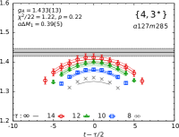
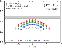
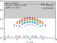
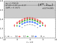
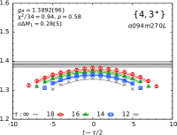
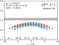
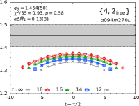
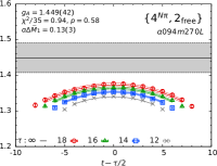
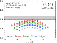
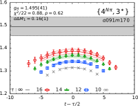
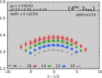
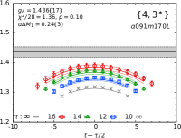
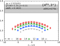
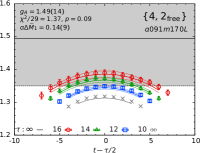
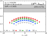
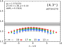
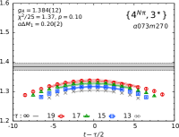
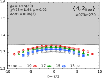
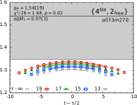
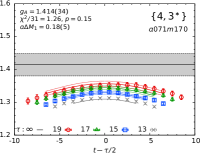
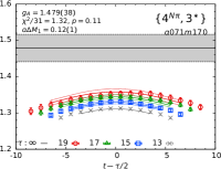
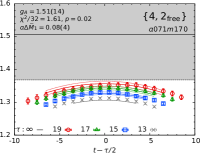
Figure 17: Each panel gives the data for the ratio ${\cal R}_{\mathcal{A}}(t,\tau)=C^{3\text{pt}}_{\mathcal{A}}(t,\tau;\bm{0},\bm{0})/C^{2\text{pt}}(\tau,\bm{0})$ defined in Eq. (19), which gives the unrenormalized axial charge $g_{A}^{u-d}$ in the limit $\tau\to\infty$, plotted as a function of $t-\tau/2$ for the four largest values of $\tau$. The data connected by lines of the same color for the three largest $\tau$ are used in the fit to get the $\tau\to\infty$ value given by the black line with its gray error band. Data at the smallest $\tau$, shown as gray crosses, are not used in the fit. The four panels in each row show the excited-state fits to the same data but with the four strategies, $\{4,3^{\ast}\}$ (left column), $\{4^{N\pi},3^{\ast}\}$ (second column), $\{4,2^{\rm free}\}$ (third column), and $\{4^{N\pi},2^{\rm free}\}$ (right column). The labels give the bare charge $g_{A}$, the $\chi^{2}/$dof of the fit, the mass gap $a\Delta M_{1}$ (or $a\Delta{\widetilde{M}}_{1}$) and the ensemble ID.

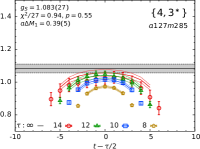
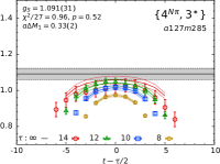
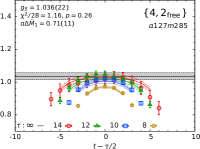
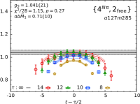
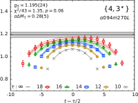
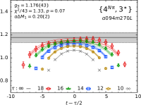
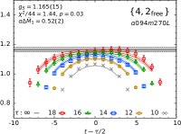
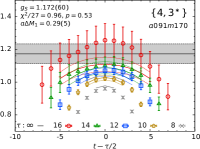
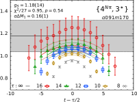
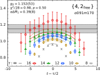
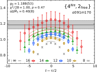
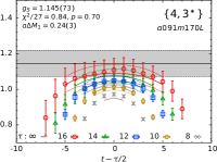
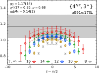
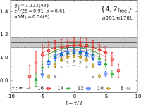
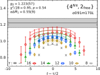
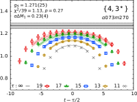
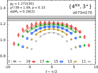
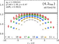
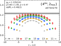
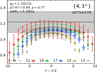
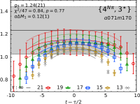
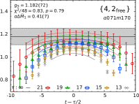
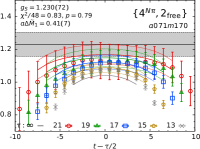
Figure 18: Each panel shows the data for the ratio defined in Eq. (19) that gives the unrenormalized scalar charge $g_{S}^{u-d}$ in the limit $\tau\to\infty$, and plotted as a function of $t-\tau/2$ for the for the five largest values of $\tau$ (four for $a127m285$). In each panel, the data with the four largest $\tau$ and connected by lines of the same color are used in the fit to get the $\tau\to\infty$ value (gray band). The rest is the same as in Fig. 17.

Appendix D Anatomy of the excited-state contamination in the charges

In this Appendix, we compare fits to the data for the three charges, $g_{A,S,T}$, in Fig. 20 to highlight (i) the differences in ESC for the $u$, $d$, $u-d$ and $u+d$ quark bilinear operator insertions and (ii) how these ESC patterns impact the extraction of the isovector and isoscalar (connected only) combinations. Data are presented for the $a071m170$ ensemble, which have the largest statistical errors. The fits are made using the $\{4,3^{\ast}\}$ strategy. We also examine the data for symmetry about $(t-\tau/2)$, monotonic convergence versus $\tau$ and the size of errors, and how these impact our ability to remove ESC.

The ESC in the axial channel is equally large in magnitude for insertion in the $u$ and $d$ quarks. It adds in the $u-d$ combination as the data have opposite signs, but cancel in $u+d$. In the case of the scalar charge, the ESC in both the $u$ and $d$ insertions are a similar fraction of the value. Thus, it adds in $u+d$. In the $u-d$ combination, there is a large cancellation; however, significant ESC remains as shown in Fig. 18. In the case of the tensor charge, the value and the ESC in the insertion in the $u$ quark is much larger, and it dominates in both the $u-d$ and the $u+d$ combinations. Overall, in the $u+d$ axial and $u-d$ scalar cases, where there is a cancellation, much higher statistical precision in the $\tau>1.5$ fm data is needed to demonstrate monotonic convergence and improve the reliability of $n$-state fits.

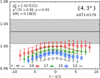
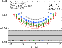
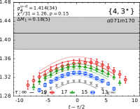
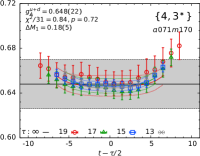
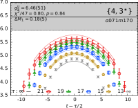
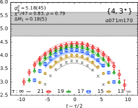
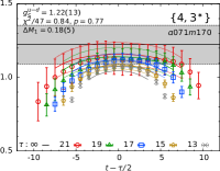
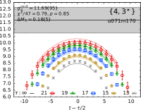
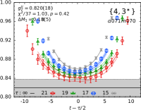
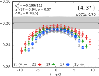
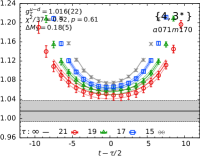
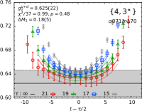
Figure 20: Data for the ratio defined in Eq. (19) for different operator insertions—on the $u$ quark (left column), $d$ quark (second column), $u-d$ combination (third column) and the connected part of the $u+d$ combination (right column)—are shown for the $a071m170$ ensemble. Data for $g_{A}$ (top row), $g_{S}$ (middle row) and $g_{T}$ (bottom row), are plotted as a function of $t-\tau/2$ for the values of $\tau$ specified in the labels. All the fits to get the $\tau\to\infty$ values are with the $\{4,3^{\ast}\}$ strategy.

Given these patterns, we made fits with the same set of ESC strategies to data with separate insertions of $u$ and $d$ quark operators. The goal was to see whether these fits, especially in the scalar channel, are more stable and the $g_{S}^{u-d}$ combination constructed from individual ESC fits has better precision. What we found, on all seven ensembles and for all three charges, is that direct fits to the $u-d$ data gave values and errors consistent with those obtained by combining results from separate fits to data with $u$ and $d$ insertions. The largest differences are in $g_{S}^{u-d}$ for the $a091m170L$ (about $1\sigma$) and $a071m170$ (about $0.5\sigma$) ensembles. This check shows that our error estimates are reasonable even in the worst cases. In short, examining the separate fits did provide a better understanding of the ESC and of the statistical precision of the fits but did not improve the estimates for the isovector charges.

Appendix E Excited states in the axial three-point functions

On a finite lattice, one has towers of eigenstates of the transfer matrix labeled by their quantum numbers. A strict identification with physical states such as $N(\bm{0})\pi({\bm{q}})$ and $N(-\bm{q})\pi({\bm{q}})$ can only be done in infinite volume and in the continuum limit. As mentioned in the text, both $N(\bm{p})\pi(-{\bm{p}})$ and $N(\bm{0})\pi({\bm{0}})\pi({\bm{0}})$ have the right quantum numbers (spin, parity, $G$-parity) to contribute to the axial channel. It is the magnitude of their couplings that decides the size of their contributions. These need to be determined nonperturbatively from fits to the three-point functions for high precision results. In such analyses, for example in the axial channel, $\chi$PT is a good guide.

In a series of papers, Bär has presented the predictions of $\chi$PT Bär, Oliver (2016, 2019a, 2019b) keeping one excited state, $N\pi$, in the analysis. At the tree level, consistent with the pion-pole dominance hypothesis, the axial current $A_{\mu}(\bm{q})$ couples through a pion with momentum $q_{\mu}$. In our setup, for the matrix elements of the three spatial $A_{i}$, the interaction with $\pi({\bm{q}})$ causes the transitions to the excited states $N(0)\to N(0)\pi(\bm{q})$ and $N(-\bm{q})\to N(-\bm{q})\pi(\bm{q})$ in addition to the desired ground state transitions $N(0)\to N(\bm{q})$ and $N(-\bm{q})\to N(\bm{0})$. These ESC arise at tree-level, depend on $\bm{q}$ and are expected to be large in the ${\widetilde{G}}_{P}$ and $G_{P}$ form factors. In addition, at the loop-level, all states with the right quantum numbers such as $N(\bm{q})\pi(\bm{0})$, $N(\bm{0})\pi(\bm{q})$, $N(\bm{0})\pi(\bm{0})\pi(\bm{0})$ and the full tower of $N(-\bm{p})\pi(\bm{p})$ states with all allowed values of $\bm{p}$ on the $\bm{p}=0$ side of the three-point function, can contribute to all three form factors. These loop-level contributions are estimated to be a few percent effect and show only a mild dependence on $\bm{p}$.

The $\{4^{N\pi},2^{\rm sim}\}$ strategy analysis of the axial form factors includes the $N\pi$ state predicted by tree-level $\chi$PT analysis but neglects the contribution of all other states that can contribute at loop-level. Compared to $\{4,3^{\ast}\}$, this changes ${\widetilde{G}}_{P}$ and $G_{P}$ by $\sim 35\%$ and $G_{A}$ by $\sim 5\%$ at the smallest $Q^{2}$ point on the $a071m170$ ensemble as shown in Fig. 21. The difference is much smaller on the $M_{\pi}\approx 270$ MeV ensembles as shown for the $a073m270$ ensemble, i.e., the effect of the $N\pi$ state increases as $Q^{2}\to 0$ and $M_{\pi}\to 0$. For the axial charge $g_{A}$ obtained from $A_{3}$, there is no tree-level contribution due to the kinematic constraint. Our analysis in Sec. VIII, including only the lowest, $N(-1)\pi(1)$ (or the approximately degenerate $N(\bm{0})\pi(\bm{0})\pi(\bm{0})$) state that can contribute at loop-level indicates that the effect could be $\sim 8\%$ for $M_{\pi}=135$ MeV. The impact of the remaining tower of excited states in either case is unknown. In this appendix, we discuss these effects and how best to proceed to remove all ESC.

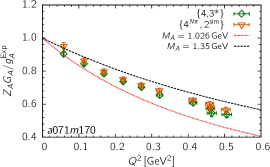
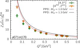
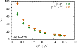
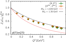
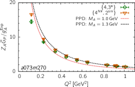
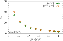
Figure 21: The form factors $Z_{A}G_{A}/g_{A}^{\rm exp}$, $Z_{A}{\widetilde{G}}_{P}/g_{A}^{\rm exp}$ and $G_{P}$ from the two strategies $\{4,3^{\ast}\}$ and $\{4^{N\pi},2^{\rm sim}\}$ are compared in each panel for the ensembles $a071m170$ (top row) and $a073m270$ (bottom row). We also show two dipole fits with $M_{A}=1.026$ and $1.35$ to $G_{A}$, and a pion-pole dominance fit to ${\widetilde{G}}_{P}$ with $G_{A}$ given by the dipole ansatz to guide the eye.

First, we discuss the evidence that multihadron states contribute. Next, we point out why it will be difficult to resolve all relevant states from fits to the two-point function. Last, we provide some thoughts on how the analysis presented in this work can be extended.

The data for the energy gaps, $a\Delta{\widetilde{M}}_{1}$ and $a\Delta{\widetilde{E}}_{1}$, obtained using three strategies $\{4,2^{\rm sim}\}$, $\{4^{N\pi},2^{A_{4}}\}$, and $\{4^{N\pi},2^{\rm sim}\}$ are presented in Fig. 22 and compared against the values obtained assuming that the excited states on the two sides of the operator are $N(\bm{q})\pi(-{\bm{q}})$ (blue dotted lines) and $N(\bm{0})\pi({\bm{q}})$ (red dotted lines), respectively. The data exhibit the following features:

• The energy gaps given by the fits to the three-point functions, $a\Delta{\widetilde{M}}_{1}$ (blue squares) and $a\Delta{\widetilde{E}}_{1}$ (red triangles), differ significantly, depending on the momentum transfer $\bm{q}$, and the difference increases with $\bm{q}$.

• The rough agreement between the blue dotted line and blue squares and the red dotted line and red triangles improves as $M_{\pi}$ decreases and indicates that $a\Delta{\widetilde{M}}_{1}$ and $a\Delta{\widetilde{E}}_{1}$ correspond to $N(\bm{q})\pi(-{\bm{q}})$ and $N(\bm{0})\pi({\bm{q}})$ excited states, respectively. The agreement was found to be even better for the physical mass ensemble investigated in Ref. Jang et al. (2020a) using the clover-on-HISQ formulation.

• The values of $a\Delta{M}_{1}$ (black filled circle) and $a\Delta{E}_{1}$ (black diamonds) obtained from $\{4\}$ and $\{4^{N\pi}\}$ fits (left versus the right two panels) to the two-point function have a smaller difference.

• The agreement between the $a\Delta{E}_{1}$ (black diamonds) from the $\{4^{N\pi}\}$ fits to the two-point function and the dotted red line showing the energy of the noninteracting $N(\bm{0})\pi(\bm{q})$ state is by construction since the latter is used as a prior for $a{E}_{1}$ in the $\{4^{N\pi}\}$ fit.

The identification of $N(\bm{0})\pi({\bm{q}})$ and $N(-\bm{q})\pi({\bm{q}})$ as the leading excited states on the two sides of the operator insertion is consistent with the predictions of chiral perturbation theory Bär, Oliver (2019a, b); Hansen and Meyer (2017).

An important consequence of the energy gaps, $a\Delta{\widetilde{M}}_{1}$ and $a\Delta{\widetilde{E}}_{1}$, being different and corresponding to different momentum dependent excited states, $N(\bm{q})\pi(-{\bm{q}})$ versus $N(\bm{0})\pi({\bm{q}})$, is that their mass gaps cannot be determined straightforwardly from fits to the two-point function. For example, for our calculations, to get the mass gaps for the ten $N(\bm{q})\pi(-{\bm{q}})$ states from the $\bm{p}=0$ correlator is unrealistic, even with a variational ansatz. As shown by the onset of the plateau in the effective mass plots in Fig. 1, the ground state dominates at $\tau\gtrsim 1$ fm, i.e., the plateau starts at $9<\tau_{\rm start}<14$ in the ensembles we have analyzed. Thus, the number of earlier time slices sensitive to, and available for determining excited-state parameters are 6–11, which restricts the analysis to a maximum of four states, including radial excitations. Second, at these short times, the contributions of the full set of excited states are still significant and even the first excited state parameters, $M_{1}$ and $E_{1}$, extracted from the fit are typically larger and $\tau_{\rm min}$ dependent. Third, these four-state fits (as well as the three-state fits) have exposed flat directions in the fit parameters leading to a large space of values with roughly similar $\chi^{2}/$dof as illustrated in Fig. 1. In short, fits to the data show many equally good solutions and the output values are heavily influenced by the priors used to stabilize the fits.

To resolve a light excited state such as $N(\bm{0})\pi(\bm{q})$, which has a mass of about 1200 MeV as $\bm{q}\to 0$, from the ground state from fits to the two-point function requires very high precision data at large enough $\tau$ by which the higher states have died out sufficiently. In our setup, this occurs for $\tau\gtrsim 1$ fm. Isolating two (actually a whole tower as $\bm{q}\to 0$) states from the “plateau” region at $\tau\gtrsim 1$ fm will be challenging. In short, our work suggests that determining the masses and amplitudes of all the needed low-lying excited states from fits to two-point functions constructed using a single nucleon or multihadron interpolating operator is unlikely in the foreseeable future.

One can improve the situation by working on anisotropic lattices (setting the spacing in the time direction much finer than in the three spatial directions to have more points to fit within the same physical time interval) and/or by using a variational approach with many nucleon interpolating operators, including relevant multihadron operators with the same quantum numbers. The two methods have been implemented together successfully in detailed calculations of the meson and baryon excited-state spectra Edwards et al. (2011). For matrix elements, however, only exploratory calculations of nucleon charges using the variational method have been performed Yoon et al. (2016); Dragos et al. (2016). Each of these approaches, unfortunately, requires additional/new simulations that are beyond the scope of the current work.

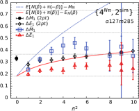
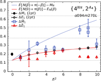
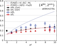
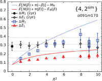
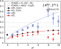
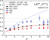
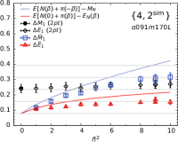
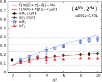
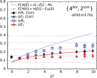
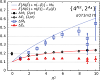
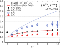
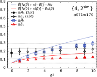
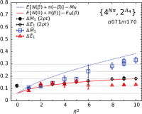
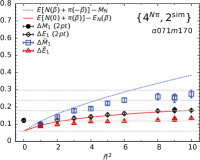
Figure 22: Mass gaps in the axial channel from various fits plotted versus the momentum transfer in units of ${\bm{n}}^{2}$ for six ensembles. The $a\Delta M_{1}$ (black filled circles) and $a\Delta E_{1}$ (black diamonds) are from fits to the two-point function using strategy $\{4\}$ (left panel), and $\{4^{N\pi}\}$ that uses a prior with a narrow width for the energy of a noninteracting $N(\bm{0})\pi({\bm{q}})$ state (middle and right panels). The output of the $\{2^{\rm sim}\}$ (or $\{2^{A_{4}}\}$) fits are $a\Delta{\widetilde{M}}_{1}$ (blue squares) and $a\Delta{\widetilde{E}}_{1}$ (red triangles). The dotted blue line is calculated assuming $a\Delta M_{1}$ is given by a noninteracting $N(\bm{q})\pi(-{\bm{q}})$ state, while the red dotted line shows the $a\Delta E_{1}$ for a noninteracting $N(\bm{0})\pi({\bm{q}})$ state.

We are, therefore, faced with the following possibilities to systematically include all the relevant excited states to get percent level precision:

• [A] Take only the ground state parameters from fits to the two-point function and leave all the excited state parameters, $\Delta{\widetilde{M}}_{i}$ and $\Delta{\widetilde{E}}_{i}$, to be determined from the three-point functions. This is the basis of our strategies $\{4^{N\pi},2^{A_{4}}\}$ and $\{4^{N\pi},2^{\rm sim}\}$, however so far we have been able to include a single excited state. To include the next, second, excited state with the current data, one could hardwire the $\Delta{\widetilde{M}}_{1}$ and $\Delta{\widetilde{E}}_{1}$, determined from a two-state fit, in a three-state fit with only $\Delta{\widetilde{M}}_{2}$ and $\Delta{\widetilde{E}}_{2}$ free. Our attempts at this failed—the $\chi^{2}$ does not decrease by two units for each additional parameter as required to satisfy the Akaike information criteria, and the parameter values have over 100% errors. We are also not able to estimate how precise the data need to be for this approach to work given the large flat regions in the $\chi^{2}$ landscape, evident already by the range of $\Delta{\widetilde{M}}_{1}$ and $\Delta{\widetilde{E}}_{1}$ values, and the large number of possible states that could contribute.

• [B] Assume, based on chiral perturbation theory, that $N(\bm{q})\pi(-{\bm{q}})$ and $N(\bm{0})\pi({\bm{q}})$ are the relevant first excited states and hardwire their noninteracting energies for $\Delta{M}_{1}$ and $\Delta{E}_{1}$ in fits to the three-point function. For the second and higher excited states, one can again resort to $\chi$PT or take the estimate of the next lowest energy level from fits to the two-point function. This approach has recently been used in Ref. Bali et al. (2020). In our case, the $\{4^{N\pi},3^{\ast}\}$ strategy is a step in this direction; however, since $\{4^{N\pi},2^{A_{4}}\}$ and $\{4^{N\pi},2^{\rm sim}\}$ do a better job of satisfying PCAC, one could add a third state with fixed $\Delta{M}_{2}$ and $\Delta{E}_{2}$ to the latter when making the fits. Our attempts at adding a third state to the $\{4^{N\pi},2^{\rm sim}\}$ fit led to both an overparameterization and essentially undetermined values for all the extra parameters.

• [C] Determine the spectrum of [multihadron] excited states in a finite box from a variational calculation of two-point functions with a large enough basis of operators and use them as priors in fits to the three-point functions. Our contention, based on the current analyses, is that, for the first excited state, the energy gaps will be close to those given by $\{4^{N\pi},2^{A_{4}}\}$ or the $\{4^{N\pi},2^{\rm sim}\}$ strategies and the fits to the three-point functions with current statistics will not be sensitive to the higher states.

In short, determining the spectrum of multiparticle excited states that contribute significantly is essential for obtaining ground state matrix elements in the axial channel. The $A_{4}$ correlator allows us to nonperturbatively identify $N\pi$ as giving the leading contribution, consistent with $\chi$PT analysis, however, more work is needed to determine the second relevant [multiparticle] excited state, which may be necessary to reach percent level precision. In Sec. XII, we show that similar issues need to be addressed in the vector channel also, but the electric and magnetic form factors are less sensitive to the values of the excited-state energies.

Appendix F Comparison of the axial form factors extracted using 4 strategies

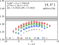
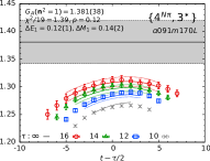
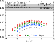
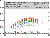
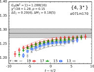
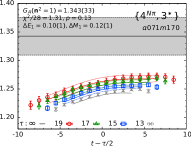
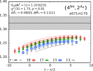
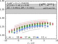
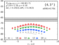
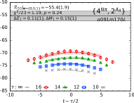
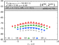
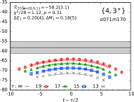
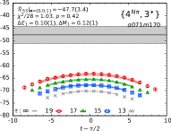
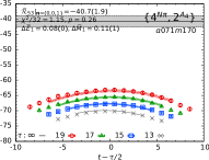
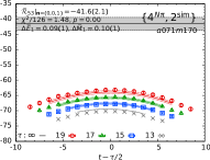
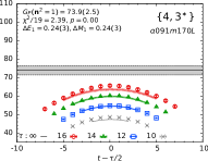
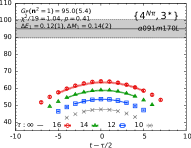
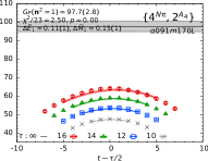
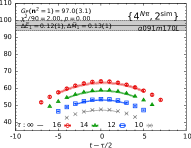
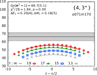
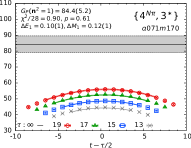
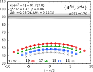
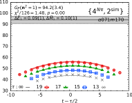
Figure 25: Matrix elements at momentum transfer ${\bm{n}}^{2}=1$ that give $G_{A}$ [from $R_{53}$ with $q_{z}=0$ defined in Eq. (22)] in rows one and two, the combination $\frac{{\widetilde{G}}_{P}}{2M_{N}}-\frac{(M+E)}{q_{3}^{2}}G_{A}$ [from $R_{53}$ with $q_{3}=(0,0,1)2\pi/La$] in rows three and four, and $G_{P}$ [from $R_{5}$ defined in Eq. (24)] in rows five and six. Data from the $a091m170L$ (rows one, three and five) and $a071m170$ (rows two, four and six) ensembles are plotted versus the shifted operator insertion time $t-\tau/2$. The four panels in each row show the data and fits from the four strategies, $\{4,3^{\ast}\}$ (left), $\{4^{N\pi},3^{\ast}\}$ (second), $\{4^{N\pi},2^{A_{4}}\}$ (third), and $\{4^{N\pi},2^{\rm sim}\}$ (right). The $y$-axis interval is chosen to be the same for each row to facilitate comparison of the result and the error. The rest is the same as in Fig. 23.

This appendix contains the data for the axial form factors obtained from four strategies used to remove ESC: $\{4,3^{\ast}\}$, $\{4^{N\pi},3^{\ast}\}$, $\{4^{N\pi},2^{A_{4}}\}$, and $\{4^{N\pi},2^{\rm sim}\}$. The renormalized axial form factors $Z_{A}G_{A}$ and $Z_{A}\widetilde{G}_{P}$ and the unrenormalized $G_{P}$ are given in Tables 18, 19 and 20, respectively. Data for the left-hand side of Eq. (29), which by the PCAC relation should equal unity, are presented in Table 21. Figure 23 shows the data for $R_{54}$, defined in Eq. (23), for six ensembles and compares the fits with the four strategies. A comparison of three matrix elements that give $\widetilde{G}_{P}$, $G_{A}$, and $G_{P}$ obtained using the four strategies is shown in Fig. 24 for the $a091m170L$ and $a071m170$ ensembles. Each row in Fig. 25 compares the results of the fits to data obtained using the four strategies to remove ESC. The six rows show data for the $a091m170L$ (rows one, three, and five) and $a071m170$ (rows two, four and six) ensembles and the three ratios: $R_{53}$ defined in Eqs (22) for two different ${\bm{n}}^{2}=1$ momentum channels, and for $R_{5}$ defined in Eq. (24). Figure 26 shows that the data for $(Q^{2}+M_{N}^{2}){\widetilde{G}}_{P}(Q^{2})$ are almost linear and monotonic versus $Q^{2}$ on all seven ensembles except at small $Q^{2}$ for the $\{4,3^{\ast}\}$, and to a lesser extent for $\{4^{N\pi},3^{\ast}\}$, strategy on the $M_{\pi}=170$ MeV ensembles (data in the upper two panels).

$\bm{n}$	$\{4,3^{*}\}$	$\{4^{N\pi},3^{*}\}$	$\{4^{N\pi},2^{A_{4}}\}$	$\{4^{N\pi},2^{\text{sim}}\}$	$\{4,3^{*}\}$	$\{4^{N\pi},3^{*}\}$	$\{4^{N\pi},2^{A_{4}}\}$	$\{4^{N\pi},2^{\text{sim}}\}$
	$a127m285$				$a094m270$
$(1,0,0)$	1.128(18)	1.136(20)	1.152(20)	1.128(22) [1.54]	1.009(20)	1.008(20)	1.014(20)	1.007(21) [1.33]
$(1,1,0)$	1.021(17)	1.023(18)	1.031(17)	1.011(18) [0.95]	0.864(23)	0.866(16)	0.884(18)	0.878(17) [1.23]
$(1,1,1)$	0.921(15)	0.918(16)	0.923(16)	0.915(17) [0.82]	0.743(24)	0.747(15)	0.763(26)	0.752(21) [1.19]
$(2,0,0)$	0.853(16)	0.848(16)	0.858(18)	0.856(19) [1.59]	0.656(40)	0.674(23)	0.714(20)	0.701(23) [1.31]
$(2,1,0)$	0.785(14)	0.779(14)	0.800(15)	0.786(16) [1.22]	0.589(26)	0.601(14)	0.619(28)	0.615(16) [0.98]
$(2,1,1)$	0.720(15)	0.712(14)	0.747(16)	0.716(16) [1.25]	0.537(26)	0.549(16)	0.588(29)	0.566(15) [1.12]
$(2,2,0)$	0.639(15)	0.635(14)	0.641(18)	0.627(18) [1.15]	0.482(32)	0.490(24)		0.519(27) [1.36]
$(2,2,1)$	0.592(16)	0.585(13)	0.608(23)	0.587(21) [1.18]	0.424(27)	0.436(23)		0.460(13) [1.26]
$(3,0,0)$	0.614(22)	0.608(25)	0.627(31)	0.618(59) [1.38]	0.542(84)	0.521(50)		0.448(19) [1.12]
$(3,1,0)$	0.570(16)	0.563(15)	0.585(17)	0.560(29) [1.39]	0.489(53)	0.485(33)		0.430(36) [1.19]
	$a094m270L$				$a091m170$
$(1,0,0)$	1.124(19)	1.134(21)	1.134(20)	1.134(20) [1.40]	1.122(19)	1.153(30)	1.167(23)	1.156(25) [1.15]
$(1,1,0)$	1.030(17)	1.031(18)	1.027(22)	1.030(18) [1.55]	1.018(17)	1.020(29)	1.028(20)	1.020(21) [1.21]
$(1,1,1)$	0.951(16)	0.945(17)	0.963(17)	0.952(17) [1.57]	0.937(16)	0.932(31)	0.948(20)	0.937(21) [1.14]
$(2,0,0)$	0.889(16)	0.876(17)	0.886(16)	0.887(16) [1.58]	0.873(17)	0.849(32)	0.894(21)	0.893(22) [1.28]
$(2,1,0)$	0.828(16)	0.815(15)	0.827(14)	0.834(15) [1.48]	0.813(16)	0.789(26)	0.828(18)	0.830(19) [1.92]
$(2,1,1)$	0.776(15)	0.761(15)	0.771(14)	0.773(15) [1.50]	0.755(16)	0.728(29)	0.764(22)	0.765(17) [1.63]
$(2,2,0)$	0.695(15)	0.680(15)	0.715(15)	0.699(14) [1.24]	0.660(18)	0.595(34)	0.741(34)	0.707(23) [2.15]
$(2,2,1)$	0.659(14)	0.647(14)	0.675(15)	0.652(14) [1.14]	0.632(17)	0.600(36)	0.678(29)	0.636(18) [1.51]
$(3,0,0)$	0.662(15)	0.637(16)	0.687(20)	0.652(19) [1.10]	0.603(28)	0.513(49)	0.753(78)	0.627(28) [1.13]
$(3,1,0)$	0.627(15)	0.601(15)	0.623(16)	0.618(18) [1.44]	0.607(21)	0.552(37)	0.638(22)	0.616(22) [1.23]
	$a091m170L$				$a073m270$
$(1,0,0)$	1.169(22)	1.208(39)	1.229(29)	1.236(30) [2.00]	1.067(14)	1.072(15)	1.061(15)	1.066(15) [1.63]
$(1,1,0)$	1.101(20)	1.119(29)	1.137(28)	1.132(29) [1.81]	0.945(13)	0.942(13)	0.941(13)	0.946(14) [1.66]
$(1,1,1)$	1.048(19)	1.059(27)	1.054(23)	1.073(29) [2.18]	0.841(13)	0.834(12)	0.847(12)	0.850(12) [1.29]
$(2,0,0)$	0.972(19)	0.945(27)	1.013(31)	0.997(26) [1.40]	0.760(14)	0.750(13)	0.781(12)	0.774(12) [1.18]
$(2,1,0)$	0.930(18)	0.900(25)	0.971(29)	0.956(20) [2.12]	0.699(13)	0.691(11)	0.725(12)	0.712(11) [2.25]
$(2,1,1)$	0.889(18)	0.851(25)	0.933(29)	0.905(25) [2.68]	0.637(15)	0.637(10)	0.674(12)	0.663(10) [1.73]
$(2,2,0)$	0.806(18)	0.755(28)	0.855(29)	0.849(24) [2.42]	0.554(15)	0.559(11)	0.592(12)	0.577(11) [1.62]
$(2,2,1)$	0.772(18)	0.719(29)	0.833(29)	0.787(21) [2.36]	0.518(16)	0.529(10)	0.544(13)	0.546(11) [1.35]
$(3,0,0)$	0.766(20)	0.700(34)	0.842(31)	0.790(21) [1.99]	0.520(17)	0.521(15)	0.540(24)	0.547(16) [1.28]
$(3,1,0)$	0.735(19)	0.666(31)	0.815(29)	0.773(23) [1.98]	0.483(15)	0.487(13)	0.529(24)	0.508(12) [1.57]
	$a071m170$
$(1,0,0)$	1.154(18)	1.203(31)	1.186(23)	1.214(27) [1.48]
$(1,1,0)$	1.078(14)	1.099(22)	1.076(16)	1.103(22) [1.82]
$(1,1,1)$	1.001(14)	0.997(19)	1.002(15)	1.018(21) [1.43]
$(2,0,0)$	0.941(16)	0.930(22)	0.954(19)	0.957(20) [1.47]
$(2,1,0)$	0.897(16)	0.878(18)	0.896(14)	0.912(19) [1.92]
$(2,1,1)$	0.837(19)	0.812(19)	0.876(33)	0.871(18) [1.69]
$(2,2,0)$	0.777(19)	0.737(22)	0.813(18)	0.799(17) [1.73]
$(2,2,1)$	0.731(20)	0.703(21)	0.787(17)	0.768(18) [1.63]
$(3,0,0)$	0.697(28)	0.658(28)	0.784(21)	0.739(26) [1.67]
$(3,1,0)$	0.686(24)	0.651(22)	0.763(18)	0.722(21) [1.97]

Table 18: Data for the renormalized axial form factor $Z_{A}G_{A}(Q^{2})$ obtained using four strategies $\{4,3^{*}\}$, $\{4^{N\pi},3^{*}\}$, $\{4^{N\pi},2^{A_{4}}\}$, $\{4^{N\pi},2^{\text{sim}}\}$ for controlling excited-state contamination. The values of $Q^{2}$, given in Table 17, for a given of value of ${\bm{n}}$ are different for all seven ensembles, so only the data with the four strategies on each ensemble should be compared. No reasonable fits could be made for the four largest $Q^{2}$ points for the $a094m270$ ensemble with the $\{4^{N\pi},2^{A_{4}}\}$ strategy. The $\chi^{2}/$dof is shown only for the $\{2^{\text{sim}}\}$ fit. In other cases, the result is obtained using a two-step process—first fits are made to remove ESC and then the overdetermined set of equations is solved to get the form factors. The data are arranged by ensemble to facilitate comparison between the four strategies for each $Q^{2}$.

$\bm{n}$	$\{4,3^{*}\}$	$\{4^{N\pi},3^{*}\}$	$\{4^{N\pi},2^{A_{4}}\}$	$\{4^{N\pi},2^{\text{sim}}\}$	$\{4,3^{*}\}$	$\{4^{N\pi},3^{*}\}$	$\{4^{N\pi},2^{A_{4}}\}$	$\{4^{N\pi},2^{\text{sim}}\}$
	$a127m285$				$a094m270$
$(1,0,0)$	20.82(58)	21.99(67)	24.29(77)	23.78(76) [1.54]	14.85(88)	14.91(48)	16.46(55)	15.89(54) [1.33]
$(1,1,0)$	13.22(32)	13.73(30)	14.56(38)	14.17(33) [0.95]	8.03(27)	8.26(22)	8.79(29)	8.61(23) [1.23]
$(1,1,1)$	9.29(23)	9.40(20)	9.82(29)	9.64(24) [0.82]	5.03(27)	5.23(17)	5.92(27)	5.55(22) [1.19]
$(2,0,0)$	7.04(21)	7.12(19)	7.65(20)	7.47(24) [1.59]	3.66(29)	3.63(18)	4.03(14)	3.83(19) [1.31]
$(2,1,0)$	5.50(14)	5.52(12)	5.95(12)	5.73(15) [1.22]	2.65(17)	2.66(10)	3.05(12)	2.82(11) [0.98]
$(2,1,1)$	4.35(13)	4.27(11)	4.76(11)	4.54(14) [1.25]	2.02(20)	2.03(11)	2.45(14)	2.18(11) [1.12]
$(2,2,0)$	3.24(13)	3.19(10)	3.43(10)	3.27(13) [1.15]	1.53(19)	1.54(13)		1.74(18) [1.36]
$(2,2,1)$	2.62(10)	2.56(10)	2.86(10)	2.82(13) [1.18]	1.01(13)	1.06(12)		1.20(09) [1.26]
$(3,0,0)$	2.57(13)	2.55(16)	2.91(17)	2.69(40) [1.38]	1.49(41)	1.40(27)		1.25(11) [1.12]
$(3,1,0)$	2.28(09)	2.26(10)	2.53(12)	2.34(13) [1.39]	1.44(29)	1.37(19)		1.03(23) [1.19]
	$a094m270L$				$a091m170$
$(1,0,0)$	24.84(84)	27.72(71)	28.51(68)	28.53(68) [1.40]	24.27(67)	28.2(1.7)	32.6(1.4)	32.0(1.3) [1.15]
$(1,1,0)$	16.23(50)	17.49(37)	17.35(78)	17.39(36) [1.55]	14.79(42)	17.17(69)	17.53(50)	17.31(51) [1.21]
$(1,1,1)$	11.70(31)	12.26(27)	12.73(27)	12.30(26) [1.57]	10.20(27)	11.53(55)	11.65(29)	11.75(31) [1.14]
$(2,0,0)$	8.94(22)	9.26(23)	9.27(25)	9.34(21) [1.58]	7.52(23)	7.78(47)	8.74(23)	8.71(26) [1.28]
$(2,1,0)$	7.04(17)	7.14(15)	7.27(16)	7.38(16) [1.48]	5.94(17)	6.25(33)	6.63(15)	6.75(18) [1.92]
$(2,1,1)$	5.74(15)	5.79(14)	5.82(13)	5.99(15) [1.50]	4.84(16)	4.94(36)	5.12(30)	5.37(20) [1.63]
$(2,2,0)$	4.08(11)	4.07(11)	4.53(09)	4.25(11) [1.24]	3.22(14)	2.90(23)	4.38(30)	3.84(12) [2.15]
$(2,2,1)$	3.55(11)	3.51(11)	3.90(09)	3.70(11) [1.14]	2.95(12)	3.04(31)	3.35(14)	3.16(13) [1.51]
$(3,0,0)$	3.54(12)	3.57(13)	3.99(11)	3.64(12) [1.10]	2.79(16)	2.38(40)	3.97(40)	3.20(15) [1.13]
$(3,1,0)$	3.02(09)	2.97(10)	3.36(09)	3.20(12) [1.44]	2.53(13)	2.16(30)	2.81(12)	2.74(12) [1.23]
	$a091m170L$				$a073m270$
$(1,0,0)$	36.3(1.3)	45.3(2.8)	46.2(2.0)	45.7(2.0) [2.00]	18.48(71)	19.98(56)	20.88(44)	21.18(39) [1.63]
$(1,1,0)$	24.55(77)	29.2(1.4)	28.41(91)	28.5(1.0) [1.81]	10.98(36)	11.46(23)	11.89(22)	12.05(21) [1.66]
$(1,1,1)$	18.27(55)	21.45(96)	19.54(74)	20.40(62) [2.18]	7.41(21)	7.56(14)	7.98(16)	8.04(14) [1.29]
$(2,0,0)$	13.64(42)	14.85(71)	15.20(72)	15.07(52) [1.40]	5.38(12)	5.44(11)	5.89(13)	5.87(11) [1.18]
$(2,1,0)$	11.33(29)	12.04(43)	12.32(32)	12.34(39) [2.12]	4.20(10)	4.15(08)	4.60(08)	4.52(09) [2.25]
$(2,1,1)$	9.41(25)	9.74(38)	10.25(27)	10.23(43) [2.68]	3.35(11)	3.26(07)	3.69(07)	3.59(07) [1.73]
$(2,2,0)$	6.78(19)	6.70(30)	7.41(19)	7.55(23) [2.42]	2.35(08)	2.26(06)	2.60(05)	2.49(06) [1.62]
$(2,2,1)$	5.95(18)	5.80(31)	6.56(18)	6.35(25) [2.36]	1.99(07)	1.93(06)	2.18(05)	2.12(06) [1.35]
$(3,0,0)$	5.58(22)	5.19(38)	6.59(24)	6.22(26) [1.99]	1.96(09)	1.90(08)	2.34(19)	2.25(08) [1.28]
$(3,1,0)$	5.08(17)	4.70(30)	5.89(18)	5.77(27) [1.98]	1.71(07)	1.65(06)	1.97(14)	1.84(08) [1.57]
	$a071m170$
$(1,0,0)$	31.8(1.8)	39.4(2.7)	42.5(1.6)	43.5(1.8) [1.48]
$(1,1,0)$	20.9(1.4)	24.3(1.3)	23.12(57)	24.46(72) [1.82]
$(1,1,1)$	14.73(73)	16.46(77)	15.82(45)	16.66(46) [1.43]
$(2,0,0)$	11.37(55)	12.41(54)	12.16(54)	12.36(31) [1.47]
$(2,1,0)$	8.86(33)	9.61(35)	9.29(27)	9.79(25) [1.92]
$(2,1,1)$	7.26(31)	7.57(29)	8.08(56)	8.10(23) [1.69]
$(2,2,0)$	5.17(21)	5.27(21)	5.88(14)	5.77(14) [1.73]
$(2,2,1)$	4.50(23)	4.55(20)	5.16(12)	5.10(16) [1.63]
$(3,0,0)$	4.44(25)	4.36(27)	5.07(14)	4.79(19) [1.67]
$(3,1,0)$	3.95(23)	3.95(19)	4.53(10)	4.31(14) [1.97]

Table 19: Data for the renormalized induced pseudoscalar form factor, $Z_{A}\widetilde{G}_{P}(Q^{2})$, obtained using the four strategies $\{4,3^{*}\}$, $\{4^{N\pi},3^{*}\}$, $\{4^{N\pi},2^{A_{4}}\}$, $\{4^{N\pi},2^{\text{sim}}\}$ for controlling excited-state contamination. The rest is the same as in Table 18.

$\bm{n}$	$\{4,3^{*}\}$	$\{4^{N\pi},3^{*}\}$	$\{4^{N\pi},2^{A_{4}}\}$	$\{4^{N\pi},2^{\text{sim}}\}$	$\{4,3^{*}\}$	$\{4^{N\pi},3^{*}\}$	$\{4^{N\pi},2^{A_{4}}\}$	$\{4^{N\pi},2^{\text{sim}}\}$
	$a127m285$				$a094m270$
$(1,0,0)$	36.0(9) [3.89]	38.6(8) [1.89]	42.0(1.0) [4.74]	41.8(1.0) [1.54]	28.5(2.1) [1.11]	28.5(7) [1.09]	31.0(9) [2.48]	30.3(8) [1.33]
$(1,1,0)$	23.4(5) [2.23]	24.2(3) [1.07]	25.6(5) [2.06]	25.1(4) [0.95]	15.6(5) [1.07]	16.0(3) [0.80]	17.2(5) [0.95]	16.7(4) [1.23]
$(1,1,1)$	17.1(4) [0.98]	17.3(3) [0.87]	18.1(4) [0.55]	17.8(3) [0.82]	10.3(3) [1.00]	10.6(2) [0.95]	11.6(4) [1.14]	11.1(4) [1.19]
$(2,0,0)$	13.0(3) [1.25]	13.1(2) [0.98]	14.2(3) [0.62]	13.9(4) [1.59]	7.2(4) [1.10]	7.2(3) [1.16]	8.0(2) [1.38]	7.6(3) [1.31]
$(2,1,0)$	10.3(2) [1.35]	10.3(1) [1.22]	11.1(2) [1.19]	10.8(2) [1.22]	6.1(3) [0.99]	6.0(2) [1.03]	7.0(3) [0.91]	6.2(3) [0.98]
$(2,1,1)$	8.6(2) [1.32]	8.5(1) [1.31]	9.3(2) [1.46]	8.9(2) [1.25]	4.6(4) [1.93]	4.6(2) [1.94]	5.2(2) [1.85]	4.8(2) [1.12]
$(2,2,0)$	6.1(1) [1.08]	6.0(1) [1.05]	6.6(2) [1.14]	6.3(2) [1.15]	3.4(5) [1.08]	3.4(3) [1.09]		4.0(4) [1.36]
$(2,2,1)$	5.5(2) [0.98]	5.4(1) [0.96]	5.9(2) [1.05]	5.8(2) [1.18]	2.7(5) [1.03]	2.7(3) [1.02]		2.8(2) [1.26]
$(3,0,0)$	5.4(2) [0.68]	5.3(2) [0.65]	6.1(3) [0.57]	5.7(6) [1.38]	2.0(8) [0.69]	2.3(5) [0.68]		2.6(4) [1.12]
$(3,1,0)$	4.8(2) [1.02]	4.7(2) [1.02]	5.5(2) [1.22]	5.0(3) [1.39]	2.4(3) [1.19]	2.4(5) [1.19]		2.7(7) [1.19]
	$a094m270L$				$a091m170$
$(1,0,0)$	44.5(1.5) [3.97]	49.9(8) [1.62]	52.1(1.1) [1.55]	52.0(8) [1.40]	50.8(1.5) [2.43]	65.7(1.4) [0.92]	67.9(2.6) [1.11]	66.9(2.4) [1.15]
$(1,1,0)$	29.9(8) [2.82]	32.3(4) [1.36]	33.2(2.0) [3.33]	32.5(4) [1.55]	31.4(8) [2.84]	36.5(9) [1.46]	37.7(9) [1.12]	37.1(10) [1.21]
$(1,1,1)$	21.9(5) [2.01]	23.0(3) [1.28]	24.0(3) [2.78]	23.3(3) [1.57]	22.0(5) [2.13]	24.6(7) [0.87]	25.7(5) [0.77]	26.2(7) [1.14]
$(2,0,0)$	17.0(3) [1.32]	17.7(2) [0.99]	17.9(4) [1.05]	18.0(3) [1.58]	16.9(4) [1.05]	18.9(8) [0.61]	19.0(5) [0.72]	19.1(5) [1.28]
$(2,1,0)$	13.9(2) [1.53]	14.1(2) [0.82]	14.4(2) [1.82]	14.6(2) [1.48]	13.3(3) [1.83]	13.6(5) [1.21]	15.3(3) [1.43]	15.5(4) [1.92]
$(2,1,1)$	11.6(2) [1.47]	11.7(2) [0.94]	11.9(1) [2.56]	12.1(2) [1.50]	11.1(3) [1.35]	10.9(8) [1.14]	12.0(6) [2.12]	12.3(4) [1.63]
$(2,2,0)$	8.6(1) [0.59]	8.5(1) [0.44]	9.3(1) [0.84]	8.9(1) [1.24]	8.0(3) [1.94]	7.6(6) [1.78]	10.2(6) [2.00]	9.1(3) [2.15]
$(2,2,1)$	7.5(1) [1.26]	7.5(1) [1.07]	8.1(1) [0.96]	7.9(1) [1.14]	6.7(2) [1.32]	5.7(6) [1.13]	7.8(3) [1.85]	7.4(3) [1.51]
$(3,0,0)$	7.5(2) [0.76]	7.6(2) [0.72]	8.4(2) [0.85]	7.7(2) [1.10]	7.4(3) [1.07]	7.4(8) [1.09]	10.3(1.6) [1.43]	7.8(4) [1.13]
$(3,1,0)$	6.5(1) [1.25]	6.4(3) [0.97]	7.3(2) [1.10]	7.0(2) [1.44]	6.3(3) [1.32]	6.5(7) [1.29]	6.8(3) [1.08]	6.9(3) [1.23]
	$a091m170L$				$a073m270$
$(1,0,0)$	73.9(2.3) [2.39]	95.0(5.1) [1.04]	97.7(3.2) [2.50]	97.0(3.4) [2.00]	34.2(1.4) [3.18]	37.2(9) [1.33]	39.1(6) [2.03]	40.1(5) [1.63]
$(1,1,0)$	50.3(1.5) [2.88]	61.4(3.1) [1.54]	60.6(1.4) [1.95]	60.4(1.8) [1.81]	20.8(7) [3.20]	21.8(3) [1.58]	22.6(3) [1.09]	23.0(2) [1.66]
$(1,1,1)$	37.5(1.0) [3.48]	44.8(1.9) [2.12]	42.1(1.1) [5.28]	44.0(1.1) [2.18]	14.7(4) [2.04]	15.0(2) [1.32]	15.7(2) [0.89]	15.7(2) [1.29]
$(2,0,0)$	30.1(8) [1.52]	34.2(1.4) [1.15]	33.9(1.5) [1.02]	34.1(1.1) [1.40]	10.9(2) [2.27]	11.1(1) [1.72]	11.7(2) [1.22]	11.8(2) [1.18]
$(2,1,0)$	24.7(6) [2.07]	27.5(10) [1.45]	27.5(6) [1.57]	27.2(8) [2.12]	8.5(1) [0.99]	8.5(1) [0.91]	9.3(1) [1.68]	9.2(1) [2.25]
$(2,1,1)$	20.7(5) [1.78]	22.7(7) [1.51]	23.0(6) [1.91]	23.3(9) [2.68]	7.0(1) [1.19]	6.9(1) [1.25]	7.7(1) [1.84]	7.5(1) [1.73]
$(2,2,0)$	15.3(3) [2.41]	16.0(5) [1.99]	17.0(4) [1.98]	17.2(6) [2.42]	5.0(1) [1.03]	5.0(1) [0.94]	5.6(1) [1.97]	5.4(1) [1.62]
$(2,2,1)$	13.6(3) [1.85]	14.3(4) [1.71]	15.0(4) [1.54]	15.0(6) [2.36]	4.4(2) [0.75]	4.2(1) [0.77]	4.9(1) [1.36]	4.7(1) [1.35]
$(3,0,0)$	13.8(3) [2.10]	14.3(6) [1.91]	15.5(5) [2.04]	14.8(5) [1.99]	4.3(2) [0.94]	4.2(2) [0.95]	5.0(3) [1.26]	4.9(2) [1.28]
$(3,1,0)$	11.9(3) [1.74]	12.1(5) [1.58]	13.5(4) [2.00]	13.4(6) [1.98]	3.8(2) [0.78]	3.8(2) [0.79]	4.5(3) [1.14]	4.2(2) [1.57]
	$a071m170$
$(1,0,0)$	66.7(4.7) [1.84]	84.4(5.2) [0.90]	91.2(3.0) [1.43]	94.2(3.5) [1.48]
$(1,1,0)$	42.7(2.8) [1.98]	50.3(2.5) [1.28]	49.7(10) [6.23]	52.0(1.4) [1.82]
$(1,1,1)$	31.1(1.7) [1.68]	35.2(1.5) [1.31]	34.4(7) [3.93]	36.0(10) [1.43]
$(2,0,0)$	24.3(1.2) [1.60]	26.6(10) [1.47]	26.4(10) [1.74]	27.6(7) [1.47]
$(2,1,0)$	19.2(6) [1.97]	20.7(6) [1.64]	20.7(4) [6.03]	22.4(6) [1.92]
$(2,1,1)$	15.9(6) [1.24]	16.7(5) [1.08]	17.9(1.2) [1.58]	18.2(5) [1.69]
$(2,2,0)$	11.7(5) [1.64]	12.2(4) [1.24]	13.6(3) [1.29]	13.5(4) [1.73]
$(2,2,1)$	10.4(4) [0.68]	10.6(4) [0.57]	11.9(3) [0.89]	12.1(3) [1.63]
$(3,0,0)$	10.5(5) [1.24]	10.3(5) [1.17]	11.5(3) [1.11]	11.5(4) [1.67]
$(3,1,0)$	9.2(4) [1.19]	9.3(5) [1.16]	10.5(3) [1.31]	10.4(4) [1.97]

Table 20: Data for the unrenormalized pseudoscalar form factor $G_{P}(Q^{2})$ obtained using four strategies $\{4,3^{*}\}$, $\{4^{N\pi},3^{*}\}$, $\{4^{N\pi},2^{A_{4}}\}$, $\{4^{N\pi},2^{\text{sim}}\}$ for controlling excited-state contamination. The numbers within the square brackets are the $\chi^{2}/$dof of the fit.

$\vec{n}$	$\{4,3^{*}\}$	$\{4^{N\pi},3^{*}\}$	$\{4^{N\pi},2^{A_{4}}\}$	$\{4^{N\pi},2^{\text{sim}}\}$	$\{4,3^{*}\}$	$\{4^{N\pi},3^{*}\}$	$\{4^{N\pi},2^{A_{4}}\}$	$\{4^{N\pi},2^{\text{sim}}\}$
	$a127m285$				$a094m270$
$(1,0,0)$	0.876(21)	0.931(16)	1.007(20)	1.015(20) [1.54]	0.930(68)	0.931(21)	1.016(25)	0.992(21) [1.33]
$(1,1,0)$	0.926(19)	0.965(11)	1.014(17)	1.008(13) [0.95]	0.951(41)	0.972(16)	1.016(24)	1.000(15) [1.23]
$(1,1,1)$	0.959(23)	0.980(13)	1.019(19)	1.009(13) [0.82]	0.946(35)	0.973(19)	1.074(31)	1.025(25) [1.19]
$(2,0,0)$	0.964(28)	0.985(15)	1.049(25)	1.027(21) [1.59]	0.982(39)	0.937(26)	0.982(18)	0.950(22) [1.31]
$(2,1,0)$	0.970(26)	0.984(13)	1.033(14)	1.012(15) [1.22]	0.948(41)	0.923(21)	1.027(53)	0.954(26) [0.98]
$(2,1,1)$	0.966(31)	0.963(15)	1.021(14)	1.017(19) [1.25]	0.909(54)	0.888(30)	0.993(26)	0.921(33) [1.12]
$(2,2,0)$	1.004(45)	0.998(18)	1.063(26)	1.036(28) [1.15]	0.936(76)	0.915(50)		0.981(69) [1.36]
$(2,2,1)$	0.967(42)	0.963(21)	1.029(25)	1.050(45) [1.18]	0.794(80)	0.796(63)		0.846(47) [1.26]
$(3,0,0)$	0.916(30)	0.919(31)	1.020(42)	0.957(64) [1.38]	0.89(17)	0.86(12)		0.905(65) [1.12]
$(3,1,0)$	0.947(33)	0.955(26)	1.034(36)	0.998(73) [1.39]	1.04(12)	0.984(88)		0.86(13) [1.19]
	$a094m270L$				$a091m170$
$(1,0,0)$	0.858(29)	0.957(17)	0.991(13)	0.991(10) [1.40]	0.723(19)	0.856(36)	0.945(28)	0.938(25) [1.15]
$(1,1,0)$	0.914(29)	0.992(14)	0.998(34)	0.989(08) [1.55]	0.824(25)	0.968(29)	0.983(21)	0.978(20) [1.21]
$(1,1,1)$	0.939(26)	0.996(13)	1.017(10)	0.994(08) [1.57]	0.859(22)	0.988(36)	0.986(19)	1.007(19) [1.14]
$(2,0,0)$	0.947(24)	1.001(13)	0.993(15)	0.999(10) [1.58]	0.862(24)	0.937(37)	0.990(18)	0.988(19) [1.28]
$(2,1,0)$	0.949(25)	0.984(11)	0.988(11)	0.994(08) [1.48]	0.881(25)	0.967(39)	0.982(15)	0.996(18) [1.92]
$(2,1,1)$	0.952(25)	0.983(13)	0.977(12)	1.001(10) [1.50]	0.905(27)	0.965(50)	0.959(35)	1.001(26) [1.63]
$(2,2,0)$	0.946(27)	0.969(14)	1.022(09)	0.985(12) [1.24]	0.877(35)	0.888(56)	1.071(51)	0.983(24) [2.15]
$(2,2,1)$	0.951(32)	0.963(17)	1.020(12)	1.006(18) [1.14]	0.921(39)	1.001(74)	0.986(25)	0.992(36) [1.51]
$(3,0,0)$	0.940(32)	0.992(19)	1.025(16)	0.989(23) [1.10]	0.923(51)	0.94(12)	1.058(08)	1.020(41) [1.13]
$(3,1,0)$	0.920(26)	0.948(18)	1.036(22)	0.998(27) [1.44]	0.908(46)	0.867(88)	0.963(27)	0.972(36) [1.23]
	$a091m170L$				$a073m270$
$(1,0,0)$	0.710(22)	0.897(44)	0.903(22)	0.889(22) [2.00]	0.855(33)	0.926(21)	0.980(10)	0.993(06) [1.63]
$(1,1,0)$	0.811(25)	0.986(48)	0.947(18)	0.952(22) [1.81]	0.909(34)	0.955(16)	0.993(09)	1.001(06) [1.66]
$(1,1,1)$	0.861(25)	1.034(42)	0.952(21)	0.977(17) [2.18]	0.936(33)	0.965(14)	1.002(10)	1.004(06) [1.29]
$(2,0,0)$	0.884(27)	1.027(51)	0.975(29)	0.985(20) [1.40]	0.935(19)	0.960(10)	0.997(12)	1.004(08) [1.18]
$(2,1,0)$	0.917(26)	1.041(44)	0.985(15)	0.999(21) [2.12]	0.944(25)	0.946(10)	0.998(08)	0.998(09) [2.25]
$(2,1,1)$	0.926(25)	1.034(40)	0.988(17)	1.019(26) [2.68]	0.959(38)	0.933(14)	0.997(09)	0.987(10) [1.73]
$(2,2,0)$	0.934(25)	1.019(41)	0.991(17)	1.016(18) [2.42]	0.969(41)	0.925(14)	1.004(09)	0.984(15) [1.62]
$(2,2,1)$	0.946(27)	1.022(45)	0.992(18)	1.019(30) [2.36]	0.962(40)	0.912(17)	1.001(12)	0.974(18) [1.35]
$(3,0,0)$	0.900(26)	0.950(45)	0.989(22)	0.994(28) [1.99]	0.939(32)	0.910(25)	1.077(76)	1.025(19) [1.28]
$(3,1,0)$	0.928(25)	0.978(44)	0.994(20)	1.027(31) [1.98]	0.963(34)	0.919(22)	1.010(44)	0.980(36) [1.57]
	$a071m170$
$(1,0,0)$	0.723(46)	0.885(45)	0.968(23)	0.972(25) [1.48]
$(1,1,0)$	0.833(59)	0.971(44)	0.950(14)	0.979(17) [1.82]
$(1,1,1)$	0.878(54)	1.004(43)	0.964(17)	0.998(15) [1.43]
$(2,0,0)$	0.915(57)	1.029(39)	0.985(28)	1.001(14) [1.47]
$(2,1,0)$	0.898(41)	1.012(33)	0.961(16)	0.998(13) [1.92]
$(2,1,1)$	0.920(45)	1.006(33)	0.995(34)	1.004(15) [1.69]
$(2,2,0)$	0.892(30)	0.976(29)	0.987(15)	0.987(13) [1.73]
$(2,2,1)$	0.914(34)	0.976(31)	0.990(15)	1.004(15) [1.63]
$(3,0,0)$	0.956(61)	1.007(47)	0.981(16)	0.984(18) [1.67]
$(3,1,0)$	0.934(48)	1.000(36)	0.978(16)	0.986(19) [1.97]

Table 21: Check of the PCAC relation between the axial and pseudoscalar form factors given in Eq. (29) for four strategies used to remove ESC. Since PCAC is an operator relation, deviations from unity should only be due to discretization errors.

Appendix G Comparison of electric and magnetic form factors extracted using 4 strategies

In this appendix, we show in Figs. 27, 28 and 29 the ratios defined in Eqs. (25)–(27) that give $G_{E}^{V_{4}}$, $G_{E}^{V_{i}}$, and $G_{M}^{V_{i}}$. The four panels in each row show the results for the ground state matrix element obtained using the four ESC strategies, $\{4,3^{*}\}$, $\{4^{N\pi},3^{*}\}$, $\{4,2^{\rm sim}\}$, $\{4^{N\pi},2^{\text{sim}}\}$. The renormalized electric and magnetic form factors are given in Tables 22, 23, and 24. Each panel in Figs. 30 and 31 shows the dipole, Padé and $z$-expansion fits to these data and gives the values of $\mathop{\langle r_{E}^{2}\rangle}\nolimits,\ \mathop{\langle r_{M}^{2}\rangle}\nolimits,\ \mu$ obtained. Data from the four strategies are shown in the four rows in each figure, and for the $a091m170L$ and $a071m170$ ensembles in the two figures.

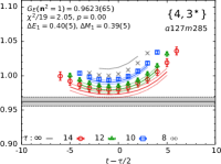
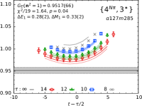
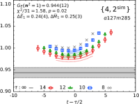
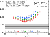
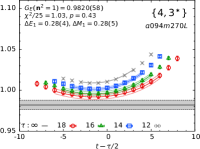
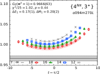
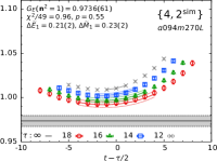
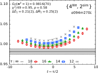
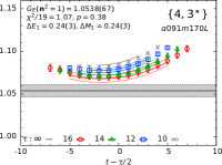
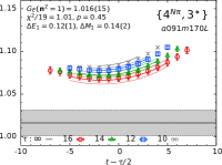
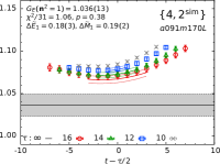
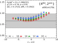
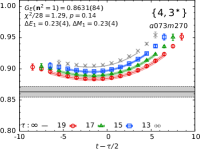
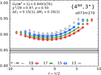
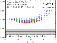
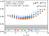
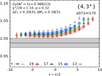
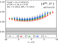
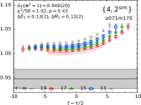
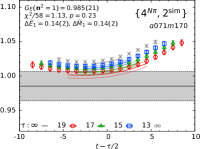
Figure 27: $G_{E}({\bm{n}}=(1,0,0))$ obtained from the ratio $R_{4}$ defined in Eq. (27) for five ensembles plotted versus the shifted operator insertion point $t-\tau/2$. The panels in the left column show the fits with $\{4,3^{\ast}\}$, the second with $\{4^{N\pi},3^{\ast}\}$, the third with $\{4,2^{\rm sim}\}$ and the right column with $\{4^{N\pi},2^{\rm sim}\}$ strategies. The interval along the $y$-axis is the same for a given row to facilitate comparison of the result and the error. The rest is the same as in Fig. 23.

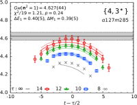
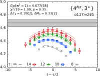
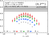
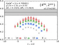
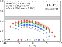
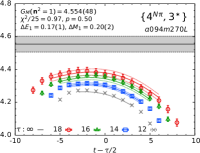
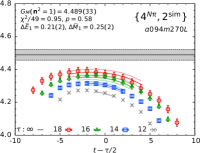
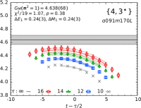
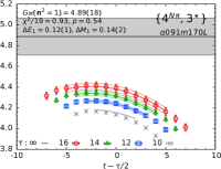
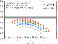
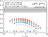
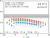
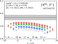
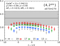
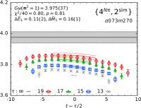
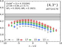
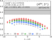
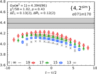
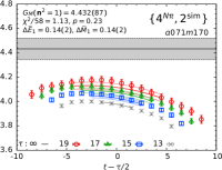
Figure 29: $G_{M}({\bm{n}}=(1,0,0))$, obtained from $\Re V_{i}$ [see Eq. (25)] plotted versus the shifted operator insertion point $t-\tau/2$. The rest is the same as in Fig. 23.

$\bm{n}$	$a127m285$	$a094m270$	$a094m270L$	$a091m170$	$a091m170L$	$a073m270$	$a071m170$
	Strategy $\{4,3^{\ast}\}$
$(1,0,0)$	0.764(05)[2.05]	0.642(20)[1.18]	0.817(04)[1.03]	0.791(06)[1.06]	0.870(05)[1.07]	0.737(07)[1.29]	0.845(11)[1.10]
$(1,1,0)$	0.609(06)[1.21]	0.461(21)[1.56]	0.680(06)[0.90]	0.643(08)[1.04]	0.764(06)[0.90]	0.569(11)[0.99]	0.723(15)[1.17]
$(1,1,1)$	0.495(08)[1.47]	0.356(16)[0.95]	0.576(08)[1.32]	0.541(09)[0.63]	0.679(07)[0.79]	0.454(12)[1.35]	0.622(18)[1.25]
$(2,0,0)$	0.417(08)[1.04]	0.245(21)[0.91]	0.499(08)[1.03]	0.464(10)[0.95]	0.607(08)[1.71]	0.376(09)[1.16]	0.548(20)[0.91]
$(2,1,0)$	0.356(08)[1.01]	0.214(14)[1.02]	0.436(08)[1.44]	0.401(09)[1.44]	0.546(09)[1.24]	0.312(10)[1.42]	0.488(17)[0.88]
$(2,1,1)$	0.303(10)[1.33]	0.184(11)[1.13]	0.385(08)[1.69]	0.355(09)[1.09]	0.498(09)[0.81]	0.262(11)[1.56]	0.435(18)[0.95]
$(2,2,0)$	0.234(09)[0.77]	0.137(16)[1.02]	0.310(08)[1.35]	0.276(11)[1.52]	0.414(09)[1.54]	0.196(11)[1.21]	0.364(14)[0.89]
$(2,2,1)$	0.208(10)[1.04]	0.128(14)[1.12]	0.278(08)[1.62]	0.251(09)[0.47]	0.385(09)[0.91]	0.176(09)[2.24]	0.333(13)[0.62]
$(3,0,0)$	0.212(10)[1.23]	0.094(43)[1.33]	0.284(08)[1.31]	0.236(16)[1.11]	0.384(09)[1.26]	0.180(09)[0.97]	0.319(18)[0.52]
$(3,1,0)$	0.188(09)[0.78]	0.125(24)[1.41]	0.261(07)[1.31]	0.222(11)[1.42]	0.353(09)[1.35]	0.156(08)[1.07]	0.301(14)[0.48]
	Strategy $\{4^{N\pi},3^{\ast}\}$
$(1,0,0)$	0.755(05)[1.64]	0.643(09)[1.15]	0.804(04)[1.02]	0.750(10)[0.94]	0.839(11)[1.01]	0.725(06)[0.97]	0.815(14)[1.16]
$(1,1,0)$	0.599(05)[1.04]	0.465(07)[1.24]	0.664(05)[0.89]	0.593(09)[1.01]	0.726(13)[0.87]	0.557(06)[1.02]	0.688(14)[1.19]
$(1,1,1)$	0.487(05)[1.49]	0.357(07)[0.89]	0.559(05)[1.27]	0.492(11)[0.85]	0.632(15)[0.76]	0.442(07)[1.59]	0.584(15)[1.46]
$(2,0,0)$	0.409(05)[1.01]	0.268(10)[0.96]	0.481(05)[0.98]	0.416(12)[0.88]	0.562(16)[1.92]	0.364(06)[1.11]	0.507(16)[1.05]
$(2,1,0)$	0.350(05)[1.03]	0.224(06)[1.04]	0.422(05)[1.19]	0.353(10)[1.18]	0.499(17)[1.43]	0.306(05)[1.58]	0.448(14)[0.96]
$(2,1,1)$	0.300(05)[1.38]	0.192(07)[1.14]	0.371(05)[1.53]	0.317(12)[0.79]	0.453(17)[0.93]	0.263(05)[2.01]	0.398(14)[1.12]
$(2,2,0)$	0.233(05)[0.76]	0.141(12)[1.01]	0.302(05)[1.14]	0.230(16)[1.09]	0.372(16)[1.73]	0.201(05)[1.47]	0.328(13)[0.88]
$(2,2,1)$	0.207(05)[1.03]	0.131(10)[1.12]	0.271(05)[1.49]	0.228(14)[0.55]	0.346(15)[1.05]	0.184(04)[2.52]	0.305(11)[0.67]
$(3,0,0)$	0.207(08)[1.20]	0.122(22)[1.37]	0.269(07)[1.24]	0.213(24)[1.03]	0.342(16)[1.33]	0.184(07)[0.97]	0.295(14)[0.55]
$(3,1,0)$	0.185(07)[0.76]	0.122(27)[1.42]	0.248(06)[1.09]	0.212(17)[1.75]	0.314(15)[1.48]	0.160(06)[1.18]	0.273(12)[0.48]
	Strategy $\{4,2^{\text{sim}}\}$
$(1,0,0)$	0.749(09)[1.58]	0.603(41)[1.07]	0.810(05)[0.96]	0.778(11)[1.48]	0.856(10)[1.06]	0.713(14)[0.89]	0.811(16)[1.02]
$(1,1,0)$	0.589(14)[1.19]	0.424(52)[0.92]	0.671(07)[0.83]	0.625(19)[0.55]	0.749(12)[0.98]	0.549(11)[1.17]	0.709(10)[1.57]
$(1,1,1)$	0.481(17)[1.44]	0.362(22)[1.02]	0.562(11)[1.08]	0.539(15)[0.85]	0.658(14)[1.09]	0.450(11)[1.04]	0.625(11)[1.35]
$(2,0,0)$	0.416(14)[1.19]	0.16(15)[1.31]	0.492(09)[1.11]	0.433(27)[0.82]	0.600(14)[0.93]	0.362(18)[1.35]	0.541(30)[0.91]
$(2,1,0)$	0.350(14)[1.03]	0.218(33)[0.92]	0.407(16)[1.06]	0.347(43)[0.77]	0.533(20)[1.27]	0.311(11)[0.97]	0.488(11)[1.31]
$(2,1,1)$	0.294(17)[1.36]	0.104(44)[1.41]	0.349(24)[1.30]	0.322(32)[0.70]	0.477(17)[1.30]	0.254(21)[0.87]	0.444(12)[1.20]
$(2,2,0)$	0.236(19)[0.90]	0.158(03)[1.28]	0.281(24)[1.13]	0.232(83)[1.24]	0.393(26)[1.29]	0.180(25)[0.76]	0.347(22)[1.10]
$(2,2,1)$	0.172(61)[1.91]	0.115(24)[1.04]	0.179(60)[1.06]	0.219(47)[0.89]	0.363(23)[1.41]	0.182(17)[0.79]	0.341(11)[1.02]
$(3,0,0)$	0.08(26)[1.21]	0.062(52)[1.60]	0.242(29)[1.25]	0.224(66)[1.33]	0.368(38)[1.26]	0.177(25)[0.95]	0.322(31)[0.66]
$(3,1,0)$	0.17(15)[0.91]	0.121(04)[1.74]	0.14(16)[1.01]	0.214(39)[1.04]	0.348(19)[1.29]	0.167(16)[1.13]	0.306(20)[0.70]
	Strategy $\{4^{N\pi},2^{\text{sim}}\}$
$(1,0,0)$	0.746(11)[1.52]	0.593(43)[1.09]	0.816(06)[0.95]	0.790(15)[1.59]	0.881(27)[0.78]	0.708(13)[0.80]	0.843(18)[1.13]
$(1,1,0)$	0.590(14)[1.21]	0.427(41)[0.89]	0.676(07)[0.88]	0.641(15)[0.60]	0.771(17)[0.81]	0.551(11)[1.19]	0.724(14)[1.62]
$(1,1,1)$	0.478(19)[1.53]	0.357(21)[1.01]	0.567(15)[1.18]	0.548(11)[0.86]	0.675(14)[1.11]	0.450(10)[1.08]	0.635(12)[1.16]
$(2,0,0)$	0.416(14)[1.19]	0.216(90)[1.36]	0.494(10)[1.16]	0.441(36)[0.94]	0.615(16)[0.92]	0.364(18)[1.37]	0.559(22)[0.89]
$(2,1,0)$	0.349(15)[1.06]	0.220(26)[0.93]	0.408(18)[1.14]	0.358(48)[0.80]	0.546(14)[1.27]	0.312(11)[0.96]	0.497(10)[1.29]
$(2,1,1)$	0.295(15)[1.44]	0.112(44)[1.38]	0.351(28)[1.41]	0.336(41)[0.76]	0.488(16)[1.35]	0.259(19)[0.86]	0.453(08)[1.16]
$(2,2,0)$	0.233(16)[1.00]	0.154(04)[1.50]	0.247(31)[1.07]	0.17(16)[0.89]	0.415(19)[1.36]	0.185(23)[0.76]	0.355(18)[1.11]
$(2,2,1)$	0.169(63)[1.95]	0.135(08)[1.06]	0.177(51)[1.33]	0.219(48)[0.96]	0.373(23)[1.44]	0.186(14)[0.78]	0.348(09)[1.01]
$(3,0,0)$	0.127(70)[0.96]	0.076(76)[1.60]	0.246(56)[1.17]	0.224(64)[1.34]	0.375(36)[1.28]	0.181(22)[0.96]	0.329(27)[0.66]
$(3,1,0)$	0.04(28)[1.20]	0.132(72)[1.66]	0.211(30)[1.31]	0.246(13)[1.10]	0.347(22)[0.99]	0.166(17)[1.13]	0.313(15)[0.71]

Table 22: Data for renormalized $G_{E}^{\Re V_{4}}(Q^{2})/g_{V}$ from the seven ensembles and with the four strategies for controlling ESC. The $\chi^{2}/$dof of the fits are given within square parentheses, and are the same for the three quantities $G_{E}^{\Re V_{4}}(Q^{2})$, $G_{E}^{\Im V_{i}}(Q^{2})$ and $G_{M}^{\Re V_{i}}(Q^{2})$ in the simultaneous $\{2^{\rm sim}\}$ fits. Only data with the four strategies for a given ensemble and ${\bm{n}}$ can be compared.

$\bm{n}$	$a127m285$	$a094m270$	$a094m270L$	$a091m170$	$a091m170L$	$a073m270$	$a071m170$
	Strategy $\{4,3^{\ast}\}$
$(1,0,0)$	0.761(17)[1.20]	0.701(89)[0.96]	0.817(19)[0.90]	0.816(46)[2.36]	0.872(35)[0.88]	0.726(30)[2.99]	0.862(81)[1.00]
$(1,1,0)$	0.620(15)[1.23]	0.534(52)[1.00]	0.690(17)[0.91]	0.679(30)[1.47]	0.788(28)[0.58]	0.583(25)[2.32]	0.749(59)[1.59]
$(1,1,1)$	0.505(16)[1.24]	0.394(25)[1.20]	0.593(18)[1.51]	0.591(26)[1.37]	0.728(27)[0.85]	0.483(23)[1.86]	0.661(57)[1.04]
$(2,0,0)$	0.436(20)[0.85]	0.296(38)[1.08]	0.531(17)[1.13]	0.518(26)[0.73]	0.635(29)[0.81]	0.412(16)[1.23]	0.611(56)[1.00]
$(2,1,0)$	0.374(16)[1.48]	0.254(25)[0.92]	0.466(14)[1.19]	0.461(22)[1.27]	0.598(24)[0.81]	0.339(16)[1.15]	0.528(34)[1.11]
$(2,1,1)$	0.318(17)[1.90]	0.185(25)[1.48]	0.419(15)[1.34]	0.418(20)[0.81]	0.564(22)[1.20]	0.295(18)[1.35]	0.484(34)[0.97]
$(2,2,0)$	0.248(20)[1.54]	0.163(27)[1.25]	0.345(13)[0.98]	0.335(21)[0.96]	0.473(25)[1.07]	0.216(16)[1.11]	0.427(27)[1.16]
$(2,2,1)$	0.218(18)[1.90]	0.095(36)[1.04]	0.311(15)[0.99]	0.309(19)[0.77]	0.439(20)[0.69]	0.201(15)[1.42]	0.376(24)[0.78]
$(3,0,0)$	0.221(17)[1.43]	0.082(66)[1.20]	0.322(16)[1.31]	0.262(34)[0.92]	0.435(28)[0.87]	0.212(16)[1.04]	0.378(38)[0.60]
$(3,1,0)$	0.212(21)[0.61]	0.211(93)[1.56]	0.302(13)[1.00]	0.280(30)[1.31]	0.397(29)[1.23]	0.162(18)[0.89]	0.346(28)[0.58]
	Strategy $\{4^{N\pi},3^{\ast}\}$
$(1,0,0)$	0.725(34)[0.91]	0.635(33)[1.00]	0.823(27)[1.38]	0.94(12)[1.74]	0.91(10)[0.58]	0.669(26)[1.21]	0.910(93)[0.96]
$(1,1,0)$	0.609(15)[0.91]	0.498(20)[1.01]	0.694(20)[0.69]	0.709(63)[1.09]	0.860(69)[0.57]	0.567(15)[1.31]	0.793(56)[1.67]
$(1,1,1)$	0.505(13)[1.09]	0.375(19)[1.20]	0.601(17)[0.97]	0.624(55)[1.36]	0.802(63)[0.74]	0.477(12)[1.52]	0.707(58)[1.26]
$(2,0,0)$	0.430(15)[0.81]	0.317(23)[1.08]	0.531(17)[1.16]	0.443(51)[0.66]	0.682(62)[0.77]	0.405(12)[1.01]	0.659(51)[0.98]
$(2,1,0)$	0.371(12)[1.49]	0.259(16)[0.94]	0.471(13)[0.90]	0.490(44)[0.66]	0.639(51)[0.80]	0.343(09)[1.04]	0.528(32)[1.24]
$(2,1,1)$	0.320(11)[1.90]	0.198(18)[1.49]	0.427(13)[1.06]	0.453(45)[0.57]	0.604(44)[1.22]	0.310(09)[1.43]	0.496(35)[1.09]
$(2,2,0)$	0.250(12)[1.53]	0.167(21)[1.24]	0.353(11)[0.93]	0.351(42)[0.68]	0.492(48)[1.14]	0.233(08)[1.15]	0.423(29)[1.15]
$(2,2,1)$	0.219(13)[1.89]	0.113(26)[1.05]	0.321(13)[0.88]	0.317(52)[0.79]	0.449(38)[0.75]	0.217(10)[1.45]	0.374(31)[0.80]
$(3,0,0)$	0.217(19)[1.42]	0.095(97)[1.23]	0.319(17)[1.25]	0.198(23)[0.87]	0.432(55)[0.81]	0.220(16)[1.05]	0.402(38)[0.59]
$(3,1,0)$	0.206(23)[0.59]	0.16(12)[1.57]	0.306(18)[0.88]	0.296(72)[1.37]	0.378(54)[1.21]	0.176(17)[0.93]	0.330(42)[0.61]
	Strategy $\{4,2^{\text{sim}}\}$
$(1,0,0)$	0.778(27)[1.58]	0.585(78)[1.07]	0.820(19)[0.96]	0.815(42)[1.48]	0.858(36)[1.06]	0.729(32)[0.89]	0.916(89)[1.02]
$(1,1,0)$	0.615(19)[1.19]	0.448(48)[0.92]	0.680(18)[0.83]	0.631(36)[0.55]	0.767(28)[0.98]	0.560(19)[1.17]	0.755(54)[1.57]
$(1,1,1)$	0.488(24)[1.44]	0.379(35)[1.02]	0.569(20)[1.08]	0.550(25)[0.85]	0.690(25)[1.09]	0.458(17)[1.04]	0.653(41)[1.35]
$(2,0,0)$	0.436(17)[1.19]	0.15(16)[1.31]	0.504(15)[1.11]	0.453(35)[0.82]	0.610(24)[0.93]	0.376(20)[1.35]	0.555(61)[0.91]
$(2,1,0)$	0.359(18)[1.03]	0.225(36)[0.92]	0.419(21)[1.06]	0.388(48)[0.77]	0.562(23)[1.27]	0.326(14)[0.97]	0.522(29)[1.31]
$(2,1,1)$	0.290(26)[1.36]	0.003(04)[1.41]	0.361(28)[1.30]	0.346(39)[0.70]	0.525(22)[1.30]	0.263(24)[0.87]	0.476(26)[1.20]
$(2,2,0)$	0.241(25)[0.90]	0.170(05)[1.28]	0.292(27)[1.13]	0.239(86)[1.24]	0.424(27)[1.29]	0.197(27)[0.76]	0.398(34)[1.10]
$(2,2,1)$	0.152(94)[1.91]	0.002(04)[1.04]	0.202(64)[1.06]	0.270(39)[0.89]	0.406(22)[1.41]	0.194(18)[0.79]	0.360(20)[1.02]
$(3,0,0)$	0.09(26)[1.21]	0.002(05)[1.60]	0.258(34)[1.25]	0.282(30)[1.33]	0.406(38)[1.26]	0.193(26)[0.95]	0.338(39)[0.66]
$(3,1,0)$	0.196(84)[0.91]	0.117(09)[1.74]	0.19(13)[1.01]	0.251(45)[1.04]	0.376(25)[1.29]	0.167(20)[1.13]	0.350(23)[0.70]
	Strategy $\{4^{N\pi},2^{\text{sim}}\}$
$(1,0,0)$	0.747(25)[1.52]	0.527(62)[1.09]	0.804(17)[0.95]	0.818(55)[1.59]	0.830(49)[0.78]	0.694(33)[0.80]	0.825(56)[1.13]
$(1,1,0)$	0.608(17)[1.21]	0.434(41)[0.89]	0.680(17)[0.88]	0.650(34)[0.60]	0.805(45)[0.81]	0.556(17)[1.19]	0.759(37)[1.62]
$(1,1,1)$	0.486(21)[1.53]	0.365(26)[1.01]	0.576(24)[1.18]	0.566(22)[0.86]	0.732(39)[1.11]	0.456(15)[1.08]	0.676(29)[1.16]
$(2,0,0)$	0.434(14)[1.19]	0.21(10)[1.36]	0.506(16)[1.16]	0.470(49)[0.94]	0.649(33)[0.92]	0.378(20)[1.37]	0.582(28)[0.89]
$(2,1,0)$	0.359(16)[1.06]	0.228(30)[0.93]	0.424(23)[1.14]	0.411(48)[0.80]	0.600(26)[1.27]	0.328(13)[0.96]	0.536(18)[1.29]
$(2,1,1)$	0.298(20)[1.44]	0.003(04)[1.38]	0.367(33)[1.41]	0.369(40)[0.76]	0.560(27)[1.35]	0.270(22)[0.86]	0.490(17)[1.16]
$(2,2,0)$	0.242(20)[1.00]	0.166(03)[1.50]	0.262(33)[1.07]	0.18(17)[0.89]	0.460(25)[1.36]	0.207(23)[0.76]	0.412(25)[1.11]
$(2,2,1)$	0.161(95)[1.95]	0.04(30)[1.06]	0.177(56)[1.33]	0.287(34)[0.96]	0.431(25)[1.44]	0.201(13)[0.78]	0.370(14)[1.01]
$(3,0,0)$	0.127(98)[0.96]	0.003(09)[1.60]	0.272(53)[1.17]	0.291(27)[1.34]	0.412(41)[1.28]	0.199(23)[0.96]	0.351(29)[0.66]
$(3,1,0)$	0.15(17)[1.20]	0.109(56)[1.66]	0.251(40)[1.31]	0.282(17)[1.10]	0.401(31)[0.99]	0.168(19)[1.13]	0.358(18)[0.71]

Table 23: Data for the renormalized $G_{E}^{\Im V_{i}}(Q^{2})/g_{V}$ from the seven ensembles and with the four strategies for controlling ESC. The rest is the same as in Table 22.

$\bm{n}$	$a127m285$	$a094m270$	$a094m270L$	$a091m170$	$a091m170L$	$a073m270$	$a071m170$
	Strategy $\{4,3^{\ast}\}$
$(1,0,0)$	3.671(33)[1.21]	3.072(58)[0.71]	3.713(27)[1.04]	3.498(42)[1.27]	3.830(54)[1.07]	3.349(26)[1.39]	3.705(68)[0.84]
$(1,1,0)$	3.071(26)[1.21]	2.320(71)[0.42]	3.193(22)[0.80]	2.962(30)[0.75]	3.458(43)[1.71]	2.724(16)[0.96]	3.250(45)[1.12]
$(1,1,1)$	2.620(28)[1.18]	1.834(68)[0.62]	2.790(23)[0.91]	2.566(68)[0.93]	3.129(40)[1.53]	2.269(22)[0.88]	2.889(44)[0.97]
$(2,0,0)$	2.231(20)[0.97]	1.593(69)[1.35]	2.471(24)[1.07]	2.302(37)[0.66]	2.809(49)[1.01]	1.963(22)[1.21]	2.624(45)[0.98]
$(2,1,0)$	1.967(25)[0.67]	1.333(48)[0.84]	2.203(27)[0.81]	2.032(29)[0.75]	2.612(37)[1.53]	1.691(24)[0.91]	2.377(37)[0.99]
$(2,1,1)$	1.756(30)[1.00]	1.146(51)[1.01]	1.969(31)[1.65]	1.808(34)[1.03]	2.408(37)[1.16]	1.471(33)[1.15]	2.127(50)[0.94]
$(2,2,0)$	1.419(35)[0.85]	0.88(15)[0.85]	1.656(29)[1.12]	1.527(34)[0.73]	2.080(38)[1.27]	1.202(29)[0.90]	1.830(54)[1.18]
$(2,2,1)$	1.312(33)[1.83]	0.817(67)[0.75]	1.500(35)[1.69]	1.364(41)[1.20]	1.944(40)[1.31]	1.069(36)[0.65]	1.696(48)[1.32]
$(3,0,0)$	1.280(39)[1.21]	0.85(20)[1.46]	1.556(28)[1.01]	1.442(51)[1.27]	1.935(48)[1.34]	1.101(31)[1.05]	1.718(57)[0.77]
$(3,1,0)$	1.198(35)[0.97]	0.82(14)[1.80]	1.430(29)[1.09]	1.283(50)[0.40]	1.845(45)[1.51]	1.019(29)[1.14]	1.664(40)[0.87]
	Strategy $\{4^{N\pi},3^{\ast}\}$
$(1,0,0)$	3.711(52)[1.09]	3.054(47)[0.72]	3.787(43)[0.97]	3.69(15)[1.26]	4.04(14)[0.93]	3.365(34)[1.36]	3.82(12)[0.82]
$(1,1,0)$	3.082(33)[1.17]	2.337(40)[0.44]	3.214(36)[0.79]	2.960(86)[0.69]	3.546(95)[1.54]	2.723(21)[0.95]	3.308(77)[1.09]
$(1,1,1)$	2.614(31)[1.22]	1.842(38)[0.62]	2.785(31)[0.89]	2.535(83)[0.84]	3.148(86)[1.45]	2.254(19)[0.88]	2.896(70)[0.95]
$(2,0,0)$	2.215(29)[0.98]	1.638(51)[1.37]	2.447(31)[1.01]	2.260(92)[0.55]	2.763(85)[0.98]	1.949(21)[1.22]	2.615(66)[0.95]
$(2,1,0)$	1.949(24)[0.72]	1.356(25)[0.85]	2.162(25)[0.71]	1.983(65)[0.77]	2.521(68)[1.39]	1.679(17)[0.92]	2.346(52)[0.99]
$(2,1,1)$	1.738(24)[1.03]	1.172(31)[1.01]	1.917(25)[1.61]	1.714(73)[1.05]	2.294(66)[1.04]	1.471(17)[1.25]	2.051(54)[0.96]
$(2,2,0)$	1.402(25)[0.90]	0.895(50)[0.83]	1.617(24)[1.11]	1.439(81)[0.69]	1.924(72)[1.11]	1.211(18)[0.85]	1.733(56)[1.20]
$(2,2,1)$	1.295(27)[1.81]	0.839(43)[0.75]	1.447(24)[1.63]	1.187(78)[1.08]	1.769(74)[1.11]	1.088(19)[0.69]	1.616(54)[1.33]
$(3,0,0)$	1.255(39)[1.22]	0.879(99)[1.45]	1.516(35)[1.01]	1.44(15)[1.29]	1.797(90)[1.24]	1.109(28)[1.06]	1.670(65)[0.73]
$(3,1,0)$	1.175(32)[1.02]	0.839(80)[1.81]	1.369(29)[1.12]	1.182(93)[0.42]	1.704(81)[1.30]	1.028(25)[1.13]	1.618(56)[0.87]
	Strategy $\{4,2^{\text{sim}}\}$
$(1,0,0)$	3.769(68)[1.58]	3.088(64)[1.07]	3.739(34)[0.96]	3.563(53)[1.48]	3.792(47)[1.06]	3.368(92)[0.89]	3.759(80)[1.02]
$(1,1,0)$	3.095(41)[1.19]	2.327(76)[0.92]	3.209(28)[0.83]	2.968(57)[0.55]	3.442(36)[0.98]	2.709(23)[1.17]	3.222(43)[1.57]
$(1,1,1)$	2.608(32)[1.44]	1.865(56)[1.02]	2.799(20)[1.08]	2.562(31)[0.85]	3.147(44)[1.09]	2.260(24)[1.04]	2.876(37)[1.35]
$(2,0,0)$	2.223(28)[1.19]	1.36(29)[1.31]	2.476(24)[1.11]	2.314(30)[0.82]	2.838(39)[0.93]	1.929(33)[1.35]	2.603(62)[0.91]
$(2,1,0)$	1.975(31)[1.03]	1.345(64)[0.92]	2.179(35)[1.06]	1.951(76)[0.77]	2.619(50)[1.27]	1.687(25)[0.97]	2.377(32)[1.31]
$(2,1,1)$	1.747(44)[1.36]	0.90(21)[1.41]	1.934(49)[1.30]	1.772(69)[0.70]	2.408(39)[1.30]	1.470(53)[0.87]	2.164(32)[1.20]
$(2,2,0)$	1.445(62)[0.90]	0.965(21)[1.28]	1.606(57)[1.13]	1.571(25)[1.24]	2.057(54)[1.29]	1.170(62)[0.76]	1.821(47)[1.10]
$(2,2,1)$	1.23(18)[1.91]	0.73(15)[1.04]	1.30(14)[1.06]	1.31(14)[0.89]	1.948(51)[1.41]	1.114(47)[0.79]	1.744(32)[1.02]
$(3,0,0)$	1.14(34)[1.21]	1.66(67)[1.60]	1.486(64)[1.25]	1.43(12)[1.33]	1.929(84)[1.26]	1.104(57)[0.95]	1.743(65)[0.66]
$(3,1,0)$	1.15(54)[0.91]	0.825(14)[1.74]	1.14(39)[1.01]	1.298(75)[1.04]	1.845(52)[1.29]	1.062(35)[1.13]	1.668(41)[0.70]
	Strategy $\{4^{N\pi},2^{\text{sim}}\}$
$(1,0,0)$	3.737(67)[1.52]	3.035(88)[1.09]	3.733(29)[0.95]	3.609(56)[1.59]	3.966(78)[0.78]	3.396(35)[0.80]	3.791(77)[1.13]
$(1,1,0)$	3.086(34)[1.21]	2.312(73)[0.89]	3.207(26)[0.88]	3.000(35)[0.60]	3.548(65)[0.81]	2.709(23)[1.19]	3.267(50)[1.62]
$(1,1,1)$	2.612(35)[1.53]	1.854(58)[1.01]	2.796(25)[1.18]	2.584(32)[0.86]	3.190(54)[1.11]	2.261(24)[1.08]	2.912(41)[1.16]
$(2,0,0)$	2.216(28)[1.19]	1.49(16)[1.36]	2.476(24)[1.16]	2.314(52)[0.94]	2.882(55)[0.92]	1.932(34)[1.37]	2.646(53)[0.89]
$(2,1,0)$	1.967(32)[1.06]	1.357(49)[0.93]	2.174(35)[1.14]	1.965(82)[0.80]	2.639(41)[1.27]	1.690(25)[0.96]	2.404(32)[1.29]
$(2,1,1)$	1.741(41)[1.44]	0.98(22)[1.38]	1.930(54)[1.41]	1.796(80)[0.76]	2.425(41)[1.35]	1.482(46)[0.86]	2.189(31)[1.16]
$(2,2,0)$	1.426(57)[1.00]	0.971(20)[1.50]	1.540(68)[1.07]	1.39(27)[0.89]	2.097(48)[1.36]	1.187(52)[0.76]	1.837(45)[1.11]
$(2,2,1)$	1.20(17)[1.95]	0.843(50)[1.06]	1.22(15)[1.33]	1.29(15)[0.96]	1.957(56)[1.44]	1.126(35)[0.78]	1.761(31)[1.01]
$(3,0,0)$	1.15(16)[0.96]	2.3(1.4)[1.60]	1.48(11)[1.17]	1.43(13)[1.34]	1.937(95)[1.28]	1.115(46)[0.96]	1.762(59)[0.66]
$(3,1,0)$	0.7(1.1)[1.20]	0.86(35)[1.66]	1.355(63)[1.31]	1.354(32)[1.10]	1.830(64)[0.99]	1.065(36)[1.13]	1.683(38)[0.71]

Table 24: Data for the renormalized $G_{M}^{\Re V_{i}}(Q^{2})/g_{V}$ from the seven ensembles and with the four strategies for controlling ESC. The rest is the same as in Table 22.

Appendix H Chiral-Continuum-Finite-Volume Fits

This appendix contains the figures showing the CCFV fits made to get the results at the physical point for various analysis strategies. Figures 32–39 show the data and fits for the three isovector charges, $g_{A,S,T}^{u-d}$; the axial charge radius squared, $\langle r_{A}^{2}\rangle$; the induced pseudoscalar charge $g_{P}^{\ast}|_{{\rm Z}_{2}}$; the pion-nucleon coupling $g_{\pi NN}|_{{\rm Z}_{2}}$; the product $M_{N}g_{A}/F_{\pi}$; the pion decay constant, $F_{\pi}$; the electric and magnetic charge radius squared, $\langle r_{E}^{2}\rangle$ and $\langle r_{M}^{2}\rangle$; and the magnetic moment, $\mu^{p-n}$, respectively. The extraction of the final results from the set of CCFV fits and the assessment of additional systematic uncertainties is presented in Sec. XIII.

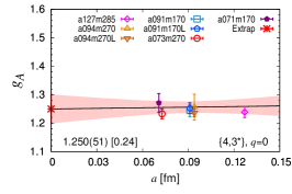
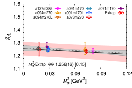
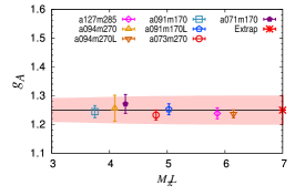
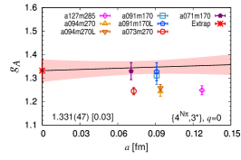
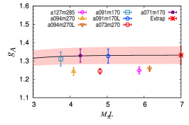
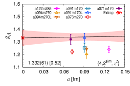
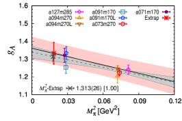
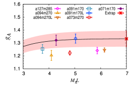
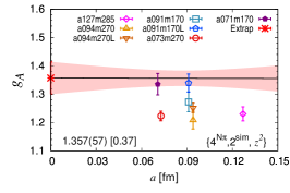
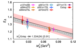
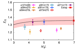
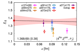
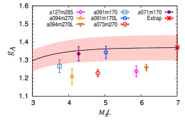
Figure 32: The CCFV extrapolation of the renormalized (${\rm Z}_{2}$ method) isovector axial charge $g_{A}^{u-d}$ for five strategies: $\{4,3^{\ast}\}$ (top row), $\{4^{N\pi},3^{\ast}\}$ (second row), $\{4,2^{\rm sim},z^{2}\}$ (third row), $\{4^{N\pi},2^{\rm sim},z^{2}\}$ (fourth row) and $\{4^{N\pi},2^{\rm sim},P_{2}\}$ (fifth row). In each panel, the result of the simultaneous fit in $\{a,M_{\pi},M_{\pi}L\}$ is shown by the pink band, and plotted versus $a$ (left panel), $M_{\pi}^{2}$ (middle) and $M_{\pi}L$ (right) with the other two variables in each case set to their physical value. The result of the CCFV fit at the physical point is shown by the red star (label Extrap) and the value and $\chi^{2}$/dof given in the left panel. The gray band is the result of a chiral fit only with the physical point marked with a black cross (label $M_{\pi}^{2}$-Extrap) and the value given in the middle panel.

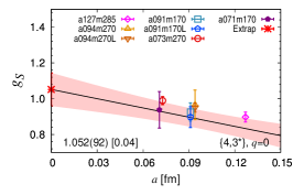
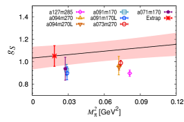
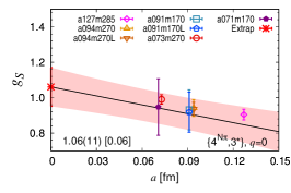
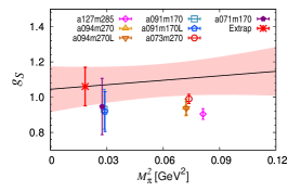
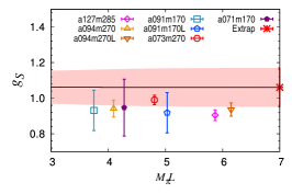
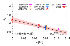
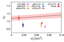
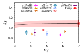
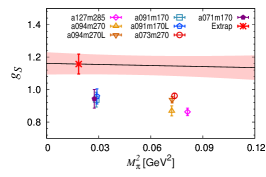
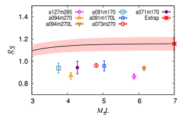
Figure 33: The CCFV extrapolation of the renormalized (${\rm Z}_{1}$ method) isovector scalar charge $g_{S}^{u-d}$ for the four strategies, to remove ESC: $\{4,3^{\ast}\}$ (top row), $\{4^{N\pi},3^{\ast}\}$ (second row), $\{4,2^{\rm free}\}$ (third row) and $\{4^{N\pi},2^{\rm free}\}$ (bottom row). The rest is the same as in Fig. 32.

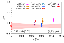
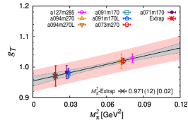
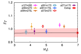
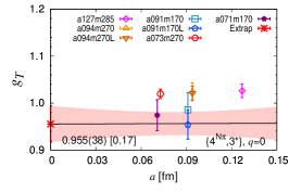
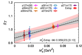
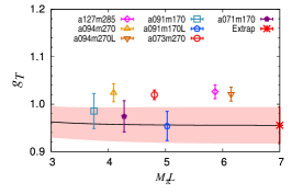
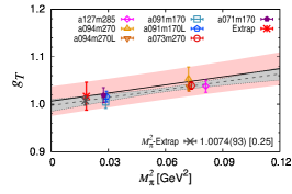
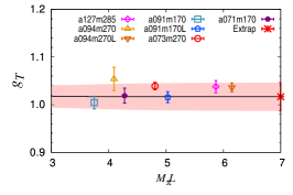
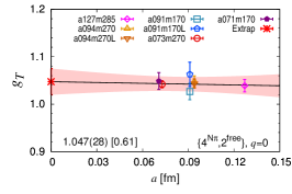
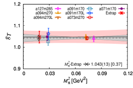
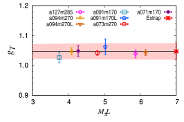
Figure 34: The CCFV extrapolation of the renormalized (${\rm Z}_{2}$ method) isovector tensor charge $g_{T}^{u-d}$ for the four strategies to remove ESC: $\{4,3^{\ast}\}$ (top row), $\{4^{N\pi},3^{\ast}\}$ (second row), $\{4,2^{\rm free}\}$ (third row) and $\{4^{N\pi},2^{\rm free}\}$ (bottom row). The rest is the same as in Fig. 32.

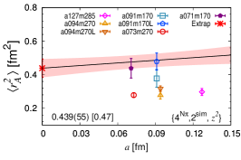
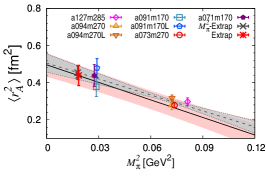
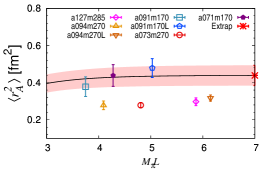
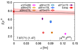
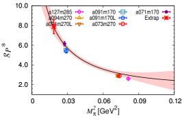
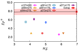
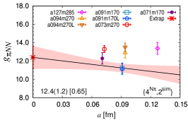
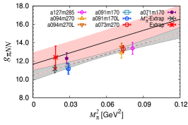
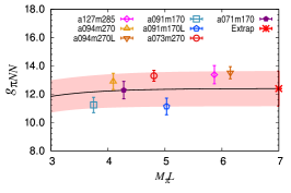
Figure 35: The CCFV extrapolation of the axial charge radius squared $\langle r_{A}^{2}\rangle$(top row), the induced pseudoscalar charge $g_{P}^{\ast}|_{{\rm Z}_{2}}$ (middle row), and the pion-nucleon coupling $g_{\pi NN}|_{{\rm Z}_{2}}$ (bottom row). The data for $\langle r_{A}^{2}\rangle$ are obtained using the $z^{2}$-fit to parameterize the $Q^{2}$ behavior. Data for $g_{P}^{\ast}|_{{\rm Z}_{2}}$ and $g_{\pi NN}|_{{\rm Z}_{2}}$ are obtained using the pion-pole dominance ansatz given in Eq. (38) to fit ${\widetilde{G}}_{P}$. Data for all three quantities are with the $\{4^{N\pi},2^{\rm sim}\}$ strategy. The rest is the same as in Fig. 32.

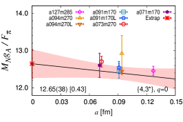
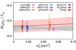
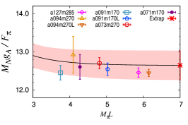
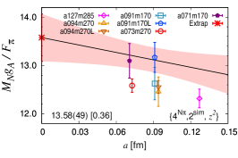
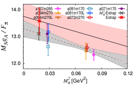
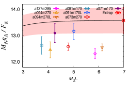
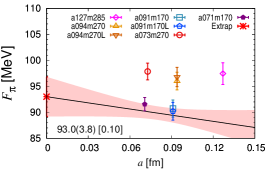
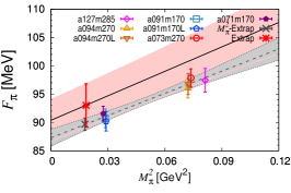
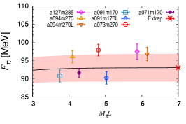
Figure 36: The CCFV extrapolation of the product $M_{N}g_{A}/F_{\pi}$ with $g_{A}$ from the $\{4,3^{\ast}\}$ (top row) and the $\{4^{N\pi},2^{\rm sim}\}$ (middle row) strategies. The bottom row shows the fit for $F_{\pi}$ renormalized using the ${\rm Z}_{1}$ method. The rest is the same as in Fig. 32.

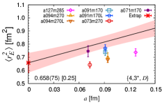
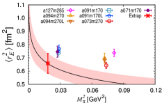
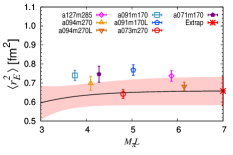
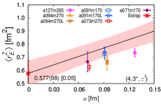
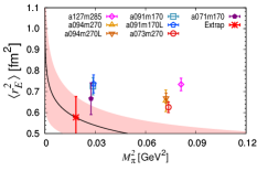
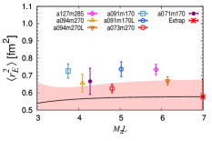
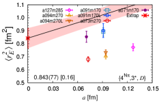
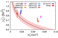
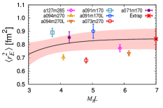
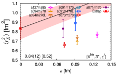
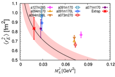
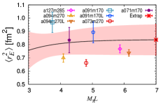
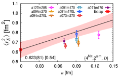
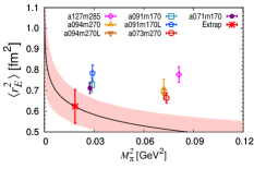
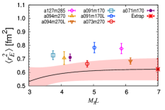
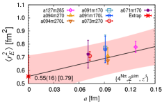
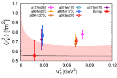
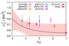
Figure 37: The CCFV extrapolation of the electric charge radius squared, $\langle r_{E}^{2}\rangle$. Data and fits are shown for three strategies, $\{4,3^{\ast}\}$ (rows one and two), $\{4^{N\pi},3^{\ast}\}$ (rows three and four), and $\{4^{N\pi},2^{\rm sim}\}$ (rows five and six). Data from the dipole (D) fit (rows one, three, and five) are compared with those from $z^{3}$ (rows two, four, and six). Each panel shows the simultaneous (CCFV) fit in the three variables, $\{a,M_{\pi},M_{\pi}L\}$, but plotted versus a single variable ($a$, or $M_{\pi}^{2}$, or $M_{\pi}L$) with the other two set to their physical value defined by $a=0$, $M_{\pi}=135$ MeV, $M_{\pi}L=\infty$. The result and the $\chi^{2}$/dof of the fit are given by the label at the bottom left in the left panel and marked by a red star (“Extrap”).

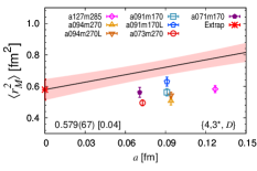
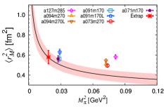
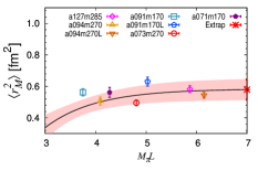
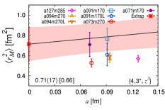
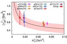
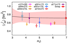
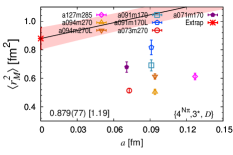
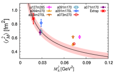
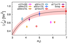
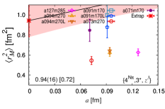
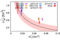
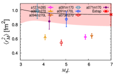
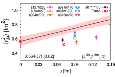
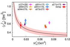
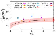
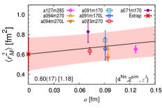
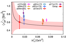
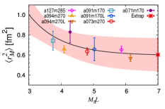
Figure 38: The CCFV extrapolation of the magnetic charge radius squared, $\langle r_{M}^{2}\rangle$. A prior for $G_{M}(0)$ was used when making the dipole, $P_{2}$ and $z^{3}$ fits to parameterize the $Q^{2}$ dependence as explained in the text. The rest is the same as in Fig. 37.

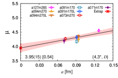
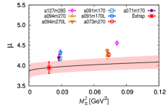
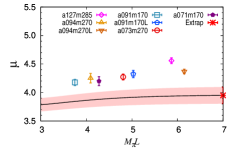
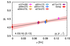
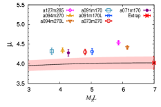
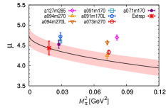
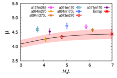
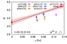
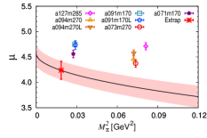
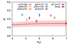
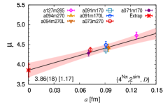
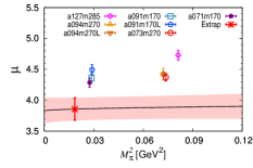
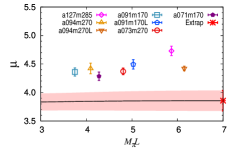
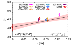
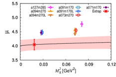
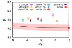
Figure 39: The CCFV extrapolation of the isovector magnetic dipole moment, $\mu^{p-n}$. A prior for $G_{M}(0)$ was used when making the dipole, $P_{2}$ and $z^{3}$ fits to parameterize the $Q^{2}$ dependence as explained in the text. The rest is the same as in Fig. 37

Appendix I Variance-covariance matrices of the fits

The fits versus $Q^{2}/4M_{N}^{2}$ and $z$ presented in Sec. XIV and the errors on the fit parameters, calculated by propagating the errors on individual points, were done using lsqfit Lepage and Gohlke (2020), which calls multifit from the GNU scientific library Galassi et al. (2001), and gvar Lepage and Hackett (2020) routines. In this appendix we provide the sampling variance-covariance matrices of the fits. The errors quoted in the main text in Sec. XIV are the square roots of the diagonal elements of these matrices.

The variance-covariance matrices for the $\{4^{N\pi},2^{\rm sim},{\widehat{P}}_{2}\}$ fit to $G_{A}$ given in Eq. (55) is

$$\blockarray{cccc}&g_{A}b_{0}b_{1}\\ \block{l(rrr)}g_{A\ }1.184\times 10^{-4}1.507\times 10^{-3}-4.499\times 10^{-3}\\ b_{0\ }1.507\times 10^{-3}3.898\times 10^{-2}-1.419\times 10^{-1}\\ b_{1\ }-4.499\times 10^{-3}-1.419\times 10^{-1}6.631\times 10^{-1}\\ \\ \,,$$ (60)

and for the $\{4^{N\pi},2^{\rm sim},{\widehat{z}}^{2}\}$ fit to $G_{A}$ given in Eq. (56) and using the notation given in Eq. (34) is

$$\blockarray{cccc}&a_{0}a_{1}a_{2}\\ \block{l(rrr)}a_{0\ }2.188\times 10^{-5}-2.238\times 10^{-5}-1.155\times 10^{-4}\\ a_{1\ }-2.238\times 10^{-5}8.549\times 10^{-4}2.769\times 10^{-3}\\ a_{2\ }-1.155\times 10^{-4}2.769\times 10^{-3}1.811\times 10^{-2}\\ \\ \,.$$ (61)

The variance-covariance matrix for the $\{4^{N\pi},3^{\ast},{\widehat{P}}_{2}\}$ fit to $G_{E}$ and $G_{M}$ given in Eq. (58) are

$$\blockarray{cccc}&g_{V}b_{0}b_{1}\\ \block{l(rrr)}g_{V}2.782\times 10^{-5}1.155\times 10^{-3}-5.206\times 10^{-3}\\ b_{0\ }1.155\times 10^{-3}8.260\times 10^{-2}-3.912\times 10^{-1}\\ b_{1\ }-5.206\times 10^{-3}-3.912\times 10^{-1}3.791\hphantom{{}\times 10^{-0}}\\ \\ \$$ (62)

and

$$\blockarray{cccc}&\mu b_{0}b_{1}\\ \block{l(rrr)}\mu 2.271\times 10^{-3}1.413\times 10^{-2}-3.931\times 10^{-2}\\ b_{0\ }1.413\times 10^{-2}1.238\times 10^{-1}-4.836\times 10^{-1}\\ b_{1\ }-3.931\times 10^{-2}-4.836\times 10^{-1}3.157\hphantom{{}\times 10^{-0}}\\ \\ \,,$$ (63)

respectively, and for the $\{4^{N\pi},3^{\ast},{\widehat{z}}^{3}\}$ fit are

$$\blockarray{ccccc}&a_{0}a_{1}a_{2}a_{3}\\ \block{l(rrrr)}a_{0\ \ }6.5178\times 10^{-6\quad}1.0374\times 10^{-5\quad}5.9814\times 10^{-6\quad}1.8014\times 10^{-5}\\ a_{1\ \ }1.0374\times 10^{-5\quad}8.1815\times 10^{-4\quad}4.6176\times 10^{-3\quad}7.3053\times 10^{-3}\\ a_{2\ \ }5.9814\times 10^{-6\quad}4.6176\times 10^{-3\quad}3.4227\times 10^{-2\quad}6.2428\times 10^{-2}\\ a_{3\ \ }1.8014\times 10^{-5\quad}7.3053\times 10^{-3\quad}6.2428\times 10^{-2\quad}1.2394\times 10^{-1}\\ \\$$ (64)

and

$$\blockarray{ccccc}&a_{0}a_{1}a_{2}a_{3}\\ \block{l(rrrr)}a_{0\ \ }1.2656\times 10^{-4\quad}3.8253\times 10^{-4\quad}9.5665\times 10^{-4\quad}1.0035\times 10^{-3}\\ a_{1\ \ }3.8253\times 10^{-4\quad}1.9869\times 10^{-2\quad}1.3524\times 10^{-1\quad}2.5216\times 10^{-1}\\ a_{2\ \ }9.5665\times 10^{-4\quad}1.3524\times 10^{-1\quad}1.3230\hphantom{{}\times 10^{-0\quad}}2.7857\hphantom{{}\times 10^{-0}}\\ a_{3\ \ }1.0035\times 10^{-3\quad}2.5216\times 10^{-1\quad}2.7857\hphantom{{}\times 10^{-0\quad}}6.4023\hphantom{{}\times 10^{-0}}\\ \\ \,,$$ (65)

respectively.

References

- Abi et al. (2018) B. Abi et al. (DUNE), “The DUNE Far Detector Interim Design Report Volume 1: Physics, Technology and Strategies,” (2018), arXiv:1807.10334 [physics.ins-det] .
- Acciarri et al. (2015) R. Acciarri et al. (DUNE), “Long-Baseline Neutrino Facility (LBNF) and Deep Underground Neutrino Experiment (DUNE),” (2015), arXiv:1512.06148 [physics.ins-det] .
- Abe et al. (2018) K. Abe et al. (Hyper-Kamiokande), “Hyper-Kamiokande Design Report,” (2018), arXiv:1805.04163 [physics.ins-det] .
- hyp (2020) “Hyper-Kamiokande,” {https://www.hyperk.org} (2020), accessed on 05/01/2020.
- Kronfeld et al. (2019) A. S. Kronfeld, D. G. Richards, W. Detmold, R. Gupta, H.-W. Lin, K.-F. Liu, A. S. Meyer, R. Sufian, and S. Syritsyn (USQCD), Eur. Phys. J. A55, 196 (2019), arXiv:1904.09931 [hep-lat] .
- Gupta et al. (2018) R. Gupta, Y.-C. Jang, B. Yoon, H.-W. Lin, V. Cirigliano, and T. Bhattacharya, Phys. Rev. D98, 034503 (2018), arXiv:1806.09006 [hep-lat] .
- Gupta et al. (2017) R. Gupta, Y.-C. Jang, H.-W. Lin, B. Yoon, and T. Bhattacharya, Phys. Rev. D96, 114503 (2017), arXiv:1705.06834 [hep-lat] .
- Jang et al. (2020a) Y.-C. Jang, R. Gupta, B. Yoon, and T. Bhattacharya, Phys. Rev. Lett. 124, 072002 (2020a), arXiv:1905.06470 [hep-lat] .
- Jang et al. (2020b) Y.-C. Jang, R. Gupta, H.-W. Lin, B. Yoon, and T. Bhattacharya, Phys. Rev. D101, 014507 (2020b), arXiv:1906.07217 [hep-lat] .
- Bazavov et al. (2013) A. Bazavov et al. (MILC Collaboration), Phys. Rev. D87, 054505 (2013), arXiv:1212.4768 [hep-lat] .
- Märkisch et al. (2019) B. Märkisch et al., Phys. Rev. Lett. 122, 242501 (2019), arXiv:1812.04666 [nucl-ex] .
- Brown et al. (2018) M. A. P. Brown et al. (UCNA), Phys. Rev. C97, 035505 (2018), arXiv:1712.00884 [nucl-ex] .
- Mendenhall et al. (2013) M. P. Mendenhall et al. (UCNA Collaboration), Phys. Rev. C87, 032501 (2013), arXiv:1210.7048 [nucl-ex] .
- Mund et al. (2013) D. Mund, B. Maerkisch, M. Deissenroth, J. Krempel, M. Schumann, H. Abele, A. Petoukhov, and T. Soldner, Phys. Rev. Lett. 110, 172502 (2013), arXiv:1204.0013 [hep-ex] .
- Bhattacharya et al. (2012) T. Bhattacharya, V. Cirigliano, S. D. Cohen, A. Filipuzzi, M. Gonzalez-Alonso, et al., Phys. Rev. D85, 054512 (2012), arXiv:1110.6448 [hep-ph] .
- Edwards et al. (2016) R. Edwards, R. Gupta, B. Joó, K. Orginos, D. Richards, F. Winter, and B. Yoon, “U.S. 2+1 flavor clover lattice generation program,” (2016), unpublished.
- Yoon et al. (2016) B. Yoon et al., Phys. Rev. D93, 114506 (2016), arXiv:1602.07737 [hep-lat] .
- Yoon et al. (2017) B. Yoon et al., Phys. Rev. D 95, 074508 (2017), arXiv:1611.07452 [hep-lat] .
- DeGrand and Rossi (1990) T. A. DeGrand and P. Rossi, Comput. Phys. Commun. 60, 211 (1990).
- Aoki et al. (2020) S. Aoki et al. (Flavour Lattice Averaging Group), Eur. Phys. J. C 80, 113 (2020), arXiv:1902.08191 [hep-lat] .
- Tanabashi et al. (2018) M. Tanabashi et al. (Particle Data Group), Phys. Rev. D 98, 030001 (2018).
- Kelly (2004) J. J. Kelly, Phys. Rev. C 70, 068202 (2004).
- Xiong et al. (2019) W. Xiong et al., Nature 575, 147 (2019).
- Bali, Gunnar S. and Collins, Sara and Schäfer, Andreas (2010) Bali, Gunnar S. and Collins, Sara and Schäfer, Andreas, Comput. Phys. Commun. 181, 1570 (2010), arXiv:0910.3970 [hep-lat] .
- Blum et al. (2013) T. Blum, T. Izubuchi, and E. Shintani, Phys. Rev. D88, 094503 (2013), arXiv:1208.4349 [hep-lat] .
- Bratt et al. (2010) J. D. Bratt et al. (LHPC Collaboration), Phys. Rev. D82, 094502 (2010), arXiv:1001.3620 [hep-lat] .
- Akaike (1974) H. Akaike, IEEE Transactions on Automatic Control 19, 716 (1974).
- Güsken, S. and Löw, U. and Mütter, K.H. and Sommer, R. and Patel, A. and Schilling, K. (1989) Güsken, S. and Löw, U. and Mütter, K.H. and Sommer, R. and Patel, A. and Schilling, K., Phys. Lett. B227, 266 (1989).
- Gupta et al. (2021) R. Gupta, S. Park, M. Hoferichter, E. Mereghetti, B. Yoon, and T. Bhattacharya, Phys. Rev. Lett. 127, 242002 (2021), arXiv:2105.12095 [hep-lat] .
- Bär, Oliver (2016) Bär, Oliver, Phys. Rev. D94, 054505 (2016), arXiv:1606.09385 [hep-lat] .
- Bär, O. (2018) Bär, O., Phys. Rev. D97, 094507 (2018), arXiv:1802.10442 [hep-lat] .
- Hoferichter et al. (2016) M. Hoferichter, B. Kubis, J. Ruiz de Elvira, H. W. Hammer, and U. G. Meißner, Eur. Phys. J. A 52, 331 (2016), arXiv:1609.06722 [hep-ph] .
- Martinelli et al. (1995) G. Martinelli, C. Pittori, C. T. Sachrajda, M. Testa, and A. Vladikas, Nucl. Phys. B445, 81 (1995), arXiv:hep-lat/9411010 [hep-lat] .
- Sturm et al. (2009) C. Sturm, Y. Aoki, N. H. Christ, T. Izubuchi, C. T. C. Sachrajda, et al., Phys. Rev. D80, 014501 (2009), arXiv:0901.2599 [hep-ph] .
- Bär, Oliver (2019a) Bär, Oliver, Phys. Rev. D 99, 054506 (2019a), arXiv:1812.09191 [hep-lat] .
- Bär, Oliver (2019b) Bär, Oliver, Phys. Rev. D 100, 054507 (2019b), arXiv:1906.03652 [hep-lat] .
- Goldberger and Treiman (1958) M. L. Goldberger and S. B. Treiman, Phys. Rev. 111, 354 (1958).
- Bernard, Veronique and Elouadrhiri, Latifa and Meißner, Ulf-G. (2002) Bernard, Veronique and Elouadrhiri, Latifa and Meißner, Ulf-G., J. Phys. G 28, R1 (2002), arXiv:hep-ph/0107088 .
- Navarro Pérez et al. (2017) R. Navarro Pérez, J. E. Amaro, and E. Ruiz Arriola, Phys. Rev. C 95, 064001 (2017), arXiv:1606.00592 [nucl-th] .
- Reinert et al. (2021) P. Reinert, H. Krebs, and E. Epelbaum, Phys. Rev. Lett. 126, 092501 (2021), arXiv:2006.15360 [nucl-th] .
- Baru et al. (2011) V. Baru, C. Hanhart, M. Hoferichter, B. Kubis, A. Nogga, and D. R. Phillips, Nucl. Phys. A872, 69 (2011), arXiv:1107.5509 [nucl-th] .
- Smith and Moniz (1972) R. A. Smith and E. J. Moniz, Nucl. Phys. B43, 605 (1972), [Erratum: Nucl. Phys. B101,547(1975)].
- Lepage and Brodsky (1980) G. P. Lepage and S. J. Brodsky, Phys. Rev. D22, 2157 (1980).
- Hill and Paz (2010) R. J. Hill and G. Paz, Phys. Rev. D82, 113005 (2010), arXiv:1008.4619 [hep-ph] .
- Bhattacharya et al. (2011) B. Bhattacharya, R. J. Hill, and G. Paz, Phys. Rev. D84, 073006 (2011), arXiv:1108.0423 [hep-ph] .
- Meyer et al. (2016) A. S. Meyer, M. Betancourt, R. Gran, and R. J. Hill, Phys. Rev. D93, 113015 (2016), arXiv:1603.03048 [hep-ph] .
- Aguilar-Arevalo et al. (2010) A. A. Aguilar-Arevalo et al. (MiniBooNE), Phys. Rev. D81, 092005 (2010), arXiv:1002.2680 [hep-ex] .
- Lynn et al. (2019) J. E. Lynn, I. Tews, S. Gandolfi, and A. Lovato, Ann. Rev. Nucl. Part. Sci. 69, 279 (2019), arXiv:1901.04868 [nucl-th] .
- Carlson et al. (2015) J. Carlson, S. Gandolfi, F. Pederiva, S. C. Pieper, R. Schiavilla, K. E. Schmidt, and R. B. Wiringa, Rev. Mod. Phys. 87, 1067 (2015), arXiv:1412.3081 [nucl-th] .
- Andreev et al. (2013) V. A. Andreev et al. (MuCap), Phys. Rev. Lett. 110, 012504 (2013), arXiv:1210.6545 [nucl-ex] .
- Andreev et al. (2015) V. A. Andreev et al. (MuCap), Phys. Rev. C91, 055502 (2015), arXiv:1502.00913 [nucl-ex] .
- Schindler et al. (2007) M. R. Schindler, T. Fuchs, J. Gegelia, and S. Scherer, Phys. Rev. C75, 025202 (2007), arXiv:nucl-th/0611083 [nucl-th] .
- Bernard, Veronique and Fearing, Harold W. and Hemmert, Thomas R. and Meißner, Ulf G. (1998) Bernard, Veronique and Fearing, Harold W. and Hemmert, Thomas R. and Meißner, Ulf G., Nucl. Phys. A 635, 121 (1998), [Erratum: Nucl. Phys. A 642, 563–563 (1998)], arXiv:hep-ph/9801297 .
- Kubis, Bastian and Meißner, Ulf-G. (2001) Kubis, Bastian and Meißner, Ulf-G., Nucl. Phys. A 679, 698 (2001), arXiv:hep-ph/0007056 .
- Gockeler, M. and Hemmert, T. R. and Horsley, R. and Pleiter, D. and Rakow, Paul E. L. and Schafer, A. and Schierholz, G. (2005) Gockeler, M. and Hemmert, T. R. and Horsley, R. and Pleiter, D. and Rakow, Paul E. L. and Schafer, A. and Schierholz, G. (QCDSF), Phys. Rev. D 71, 034508 (2005), arXiv:hep-lat/0303019 .
- Beane (2004) S. R. Beane, Phys. Rev. D 70, 034507 (2004), arXiv:hep-lat/0403015 .
- Beane and Savage (2003) S. R. Beane and M. J. Savage, Phys. Rev. D 68, 114502 (2003), arXiv:hep-lat/0306036 .
- Alexandrou et al. (2021) C. Alexandrou et al., Phys. Rev. D 103, 034509 (2021), arXiv:2011.13342 [hep-lat] .
- Alexandrou et al. (2020) C. Alexandrou, S. Bacchio, M. Constantinou, J. Finkenrath, K. Hadjiyiannakou, K. Jansen, G. Koutsou, and A. Vaquero Aviles-Casco, Phys. Rev. D 102, 054517 (2020), arXiv:1909.00485 [hep-lat] .
- Alexandrou et al. (2019) C. Alexandrou, S. Bacchio, M. Constantinou, J. Finkenrath, K. Hadjiyiannakou, K. Jansen, G. Koutsou, and A. Vaquero Aviles-Casco, Phys. Rev. D 100, 014509 (2019), arXiv:1812.10311 [hep-lat] .
- Abramczyk et al. (2020) M. Abramczyk, T. Blum, T. Izubuchi, C. Jung, M. Lin, A. Lytle, S. Ohta, and E. Shintani, Phys. Rev. D 101, 034510 (2020), arXiv:1911.03524 [hep-lat] .
- Walker-Loud et al. (2020) A. Walker-Loud et al., PoS CD2018, 020 (2020), arXiv:1912.08321 [hep-lat] .
- Chang et al. (2018) C. C. Chang et al., Nature 558, 91 (2018), arXiv:1805.12130 [hep-lat] .
- Ishikawa et al. (2018) K.-I. Ishikawa, Y. Kuramashi, S. Sasaki, N. Tsukamoto, A. Ukawa, and T. Yamazaki (PACS), Phys. Rev. D 98, 074510 (2018), arXiv:1807.03974 [hep-lat] .
- Shintani et al. (2019) E. Shintani, K.-I. Ishikawa, Y. Kuramashi, S. Sasaki, and T. Yamazaki, Phys. Rev. D 99, 014510 (2019), [Erratum: Phys. Rev. D 102, 019902 (2020)], arXiv:1811.07292 [hep-lat] .
- Tsukamoto et al. (2020) N. Tsukamoto, Y. Aoki, K.-I. Ishikawa, Y. Kuramashi, E. Shintani, S. Sasaki, and T. Yamazaki, PoS LATTICE2019, 132 (2020), arXiv:1912.00654 [hep-lat] .
- Bali et al. (2020) G. S. Bali, L. Barca, S. Collins, M. Gruber, M. Löffler, A. Schäfer, W. Söldner, P. Wein, S. Weishäupl, and T. Wurm (RQCD), JHEP 05, 126 (2020), arXiv:1911.13150 [hep-lat] .
- Harris et al. (2019) T. Harris, G. von Hippel, P. Junnarkar, H. B. Meyer, K. Ottnad, J. Wilhelm, H. Wittig, and L. Wrang, Phys. Rev. D 100, 034513 (2019), arXiv:1905.01291 [hep-lat] .
- Djukanovic et al. (2021) D. Djukanovic, T. Harris, G. von Hippel, P. M. Junnarkar, H. B. Meyer, D. Mohler, K. Ottnad, T. Schulz, J. Wilhelm, and H. Wittig, Phys. Rev. D 103, 094522 (2021), arXiv:2102.07460 [hep-lat] .
- Hasan et al. (2019) N. Hasan, J. Green, S. Meinel, M. Engelhardt, S. Krieg, J. Negele, A. Pochinsky, and S. Syritsyn, Phys. Rev. D 99, 114505 (2019), arXiv:1903.06487 [hep-lat] .
- Hasan et al. (2018) N. Hasan, J. Green, S. Meinel, M. Engelhardt, S. Krieg, J. Negele, A. Pochinsky, and S. Syritsyn, Phys. Rev. D 97, 034504 (2018), arXiv:1711.11385 [hep-lat] .
- Liang et al. (2018) J. Liang, Y.-B. Yang, T. Draper, M. Gong, and K.-F. Liu, Phys. Rev. D 98, 074505 (2018), arXiv:1806.08366 [hep-ph] .
- Aoki et al. (2021) Y. Aoki et al., “FLAG Review 2021,” (2021), arXiv:2111.09849 [hep-lat] .
- Yamanaka et al. (2018) N. Yamanaka, S. Hashimoto, T. Kaneko, and H. Ohki (JLQCD), Phys. Rev. D 98, 054516 (2018), arXiv:1805.10507 [hep-lat] .
- Bruno et al. (2015) M. Bruno et al., JHEP 02, 043 (2015), arXiv:1411.3982 [hep-lat] .
- Mondal et al. (2020) S. Mondal, R. Gupta, S. Park, B. Yoon, T. Bhattacharya, B. Joó, and F. Winter (Nucleon Matrix Elements (NME)), JHEP 21, 004 (2020), arXiv:2011.12787 [hep-lat] .
- Edwards and Joo (2005) R. G. Edwards and B. Joo (SciDAC Collaboration, LHPC Collaboration, UKQCD Collaboration), Nucl. Phys. Proc. Suppl. 140, 832 (2005), arXiv:hep-lat/0409003 [hep-lat] .
- Brannick et al. (2008) J. Brannick, R. C. Brower, M. A. Clark, J. C. Osborn, and C. Rebbi, Phys. Rev. Lett. 100, 041601 (2008), arXiv:0707.4018 [hep-lat] .
- Babich et al. (2010a) R. Babich, J. Brannick, R. C. Brower, M. A. Clark, T. A. Manteuffel, et al., Phys. Rev. Lett. 105, 201602 (2010a), arXiv:1005.3043 [hep-lat] .
- Osborn et al. (2010) J. C. Osborn, R. Babich, J. Brannick, R. C. Brower, M. A. Clark, et al., PoS LATTICE2010, 037 (2010), arXiv:1011.2775 [hep-lat] .
- Clark et al. (2010) M. A. Clark, R. Babich, K. Barros, R. C. Brower, and C. Rebbi, Comput. Phys. Commun. 181, 1517 (2010), arXiv:0911.3191 [hep-lat] .
- Babich et al. (2010b) R. Babich, M. A. Clark, and B. Joo, ACM/IEEE Int. Conf. High Performance Computing, Networking, Storage and Analysis, New Orleans (2010b), 10.1109/SC.2010.40, arXiv:1011.0024 [hep-lat] .
- Babich et al. (2011) R. Babich, M. A. Clark, B. Joo, G. Shi, R. C. Brower, and S. Gottlieb, in SC11 International Conference for High Performance Computing, Networking, Storage and Analysis Seattle, Washington, November 12-18, 2011 (2011) arXiv:1109.2935 [hep-lat] .
- Clark et al. (2016) M. A. Clark, B. Joó, A. Strelchenko, M. Cheng, A. Gambhir, and R. Brower, ACM/IEEE Int. Conf. High Performance Computing, Networking, Storage and Analysis, Salt Lake City, Utah (2016), 10.1109/SC.2010.40, arXiv:1612.07873 [hep-lat] .
- Borsanyi et al. (2012) S. Borsanyi et al., JHEP 09, 010 (2012), arXiv:1203.4469 [hep-lat] .
- Hansen and Meyer (2017) M. T. Hansen and H. B. Meyer, Nucl. Phys. B 923, 558 (2017), arXiv:1610.03843 [hep-lat] .
- Edwards et al. (2011) R. G. Edwards, J. J. Dudek, D. G. Richards, and S. J. Wallace, Phys. Rev. D 84, 074508 (2011), arXiv:1104.5152 [hep-ph] .
- Dragos et al. (2016) J. Dragos, R. Horsley, W. Kamleh, D. B. Leinweber, Y. Nakamura, P. E. L. Rakow, G. Schierholz, R. D. Young, and J. M. Zanotti, Phys. Rev. D 94, 074505 (2016), arXiv:1606.03195 [hep-lat] .
- Lepage and Gohlke (2020) P. Lepage and C. Gohlke, “Gplepage/lsqfit: Lsqfit Version 11.7,” (2020), code published in Zenodo.
- Galassi et al. (2001) M. Galassi, F. Rossi, B. Gough, M. Booth, G. Jungman, J. Theiler, and J. Davies, GNU Scientific Library: Reference Manual (Network Theory Limited, 2001).
- Lepage and Hackett (2020) P. Lepage and D. Hackett, “Gplepage/gvar: Gvar Version 11.9.1,” (2020), code published in Zenodo.