Covariate-informed latent interaction models: Addressing geographic & taxonomic bias in predicting bird-plant interactions

Abstract

Reductions in natural habitats urge that we better understand species’ interconnection and how biological communities respond to environmental changes. However, ecological studies of species’ interactions are limited by their geographic and taxonomic focus which can distort our understanding of interaction dynamics. We focus on bird-plant interactions that refer to situations of potential fruit consumption and seed dispersal. We develop an approach for predicting species’ interactions that accounts for errors in the recorded interaction networks, addresses the geographic and taxonomic biases of existing studies, is based on latent factors to increase flexibility and borrow information across species, incorporates covariates in a flexible manner to inform the latent factors, and uses a meta-analysis data set from 85 individual studies. We focus on interactions among 232 birds and 511 plants in the Atlantic Forest, and identify 5% of pairs of species with an unrecorded interaction, but posterior probability that the interaction is possible over 80%. Finally, we develop a permutation-based variable importance procedure for latent factor network models and identify that a bird’s body mass and a plant’s fruit diameter are important in driving the presence of species interactions, with a multiplicative relationship that exhibits both a thresholding and a matching behavior.

keywords: Bayesian methods; ecology; graph completion; latent factors; variable importance

1.   Introduction

Animal-plant interactions have played an important role in the generation of Earth’s biodiversity (Ehrlich & Raven, 1964). Hundreds of species form complex networks of interdependences whose structure has important implications for the stability of ecosystems (Solé & Montoya, 2001), their robustness to species extinctions (Aizen et al., 2012; Dunne et al., 2002), and their resilience in the face of environmental change (Tylianakis et al., 2008). Climate change and the reduction in species’ natural habitats necessitate that we urgently understand species’ interdependence in order to better predict how environmental changes will affect species’ equilibrium and co-existence.

Predicting and understanding species interactions is a long standing question in ecology. However, accessing all the possible interactions in a mutualistic network is a huge task that requires significant experimental effort (Jordano, 2016). Individual studies might focus on recording the interactions of only a given set of species. Even for the species under study, most measured networks are recorded in a specific geographical area where only a subset of species occurs. As a result, recorded networks are substantially incomplete and not comprehensively representative of species interactions, irrespective of the researchers’ observational effort. These individual study characteristics lead to over-representation of a subset of species and under-representation of others implying that the resulting measured networks are taxonomically and geographically biased. Even if measured networks from individual studies are compiled into one overarching network including all recorded interactions, these biases will propagate since cryptic species that occur in uncharted regions, or are not the explicit focus of the individual studies, will remain under-represented. Even though these biases and their implications are well-recognized (Báldi & McCollin, 2003; Seddon et al., 2005; Pyšek et al., 2008; Hale & Swearer, 2016), most models for species interactions do not account for them (e.g. Bartomeus, 2013). Some advances are emerging in the literature (Cirtwill et al., 2019; Weinstein & Graham, 2017; Graham & Weinstein, 2018), but the models therein do not provide a comprehensive treatment of species’ traits and phylogenetic information. Our goal is to use incomplete networks to understand whether a given bird would eat the fruit of a given plant if given the opportunity, and to learn which species traits are important in forming these interactions.

From a statistical perspective, a bird-plant interaction network can be conceptualized as a bipartite graph, where the birds and plants form separate sets of nodes, and an edge connects one node from each set. If a certain animal-plant interaction has been recorded, the corresponding edge necessarily exists. However, absence of a recorded interaction does not mean that the interaction is not possible and the networks are measured with error. Modeling the probability of connections on a graph measured without error has received a lot of attention in the statistics literature, and examples stretch across social (Newman et al., 2002; Wu et al., 2010), biological (Chen & Yuan, 2006; Bullmore & Sporns, 2009), and ecological (Croft et al., 2004; Blonder & Dornhaus, 2011) networks, among others. Since the literature on network modeling is vast, we focus on approaches for bipartite graphs. In an early approach, Skvoretz & Faust (1999) adapted the $p^{*}$ network models to the bipartite setting. Community detection in bipartite graphs (referred to as co-clustering) was first introduced in Hartigan (1972) and it has flourished in the last couple of decades (e.g., Dhillon et al., 2003; Shan & Banerjee, 2008; Wang et al., 2011; Razaee et al., 2019). Our approach is more closely related to network modeling using latent factors (Hoff et al., 2002; Handcock et al., 2007) and its extension to multilinear relationships (Hoff, 2005, 2011, 2015), where the nodes are embedded in a Euclidean space and the presence of an edge depends on the nodes’ relative distance in the latent space. Since our observed networks have missing edges, our approach also has ties to modeling noisy observed networks (Jiang et al., 2011; Wang et al., 2012; Priebe et al., 2015; Chang et al., 2022).

Our goals are to complete the bipartite graph of species interactions given the recorded, error-prone networks from individual studies, and to understand which covariates are most important for driving species interdependence. We develop a Bayesian approach to modeling the probability that a bird-plant interaction is possible based on a meta-analysis data set from 85 studies on the Atlantic Forest. The proposed approach a) models the probability of a link in the bipartite graph, b) incorporates the missingness mechanism caused by the taxonomic and geographic bias of individual studies, and the possibility that an interaction was not detected, c) uses covariate information to inform the network model and improve precision, d) employs a latent variable approach to link the model components, e) quantifies our uncertainty around the estimated graph, and f) uses posterior samples in a permutation approach to acquire a variable importance metric. To our knowledge, our approach is the first to employ latent network models for noisy networks, to use covariates to inform the latent factors via separate models instead of including them in the network model directly, and to study variable importance in latent factor models.

2.   A multi-study data set of bird–plant interactions in the Atlantic Forest

The Atlantic Forest is threatened due to overexploitation of its natural resources, and it currently includes only 12% of its original biome (Ribeiro et al., 2009). In this biome, plants rely heavily on frugivore animals for their seed dispersal, and reductions in frugivore populations lead to disruptions in the regeneration of ecosystems. To better understand species’ interactions and how biological communities respond to environmental changes, we study bird-plant interactions in the Atlantic Forest. We use an extensive data set which includes frugivore-plant interactions from 166 studies for five frugivore classes (Bello et al., 2017). A recorded interaction represents a setting where a frugivore was involved in the plant’s seed dispersal process, in that it handled a fruit in a manner that may have ended in consumption and subsequent dispersal of the seed. Other types of fruit handling that could not have led to seed dispersal were excluded from the data set, wherever this information was available. Since we focus on bird-plant interactions (excluding mammals or other classes), we maintain 85 studies that include at least one such interaction. These 85 studies recorded interactions for 232 birds and 511 plant species, but only 458 of the plant species were involved in an interaction with a bird (Supplement J includes the list of species). The number of unique recorded bird-plant interactions was 3,804.

One of the key characteristics of our data is that unobserved interactions might be possible. For an interaction to be recorded there has to exist at least one study for which both species co-occur at the study site, they interact, and the interaction was detected and recorded. However, individual studies are often limited in terms of the species or geographical area they focus on. Species-oriented studies record only a subset of the interactions that are detected: an animal-oriented study focuses on a given animal’s diet whereas a plant-oriented study focuses on learning which animals eat the fruits of a given plant. Hence, measured networks from such studies do not represent species comprehensibly and are taxonomically biased. In contrast, network studies record any interaction that is observed. However, studies of either type often focus on a small area where not all animal and plant species occur, and are hence geographically biased. As a result, a complete record of interactions is almost impossible to acquire, even for species of explicit interest.

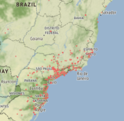
(a) Geographic bias

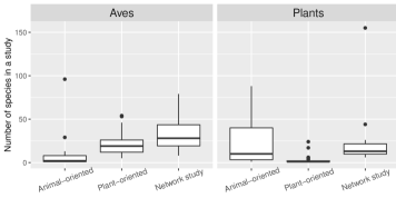
(b) Taxonomic bias

Figure 1: Geographic and Taxonomic Bias. (a) Locations of recorded interactions with reported coordinate information amounting to 68% of recorded interactions. (b) Number of unique bird and plant species with recorded interactions within each study, by study type (animal/plant-oriented, network study).

The taxonomic and geographical biases of the individual studies propagate when compiling the recorded interactions into one combined network. Since most studies are located in the southeast Atlantic Forest (see Figure 1a), interactions among species that do not co-occur in this area are less likely to be detected. Out of the eight bioregions of the Atlantic Forest biome, 45% of interactions were recorded in the Serra do Mar bioregion, and there was no recorded interaction in the São Francisco bioregion. Therefore, the combined network will over-represent species that occur in the regions that are heavily studied and under-represent species that do not, implying that the combined network is itself geographically biased. Out of the 85 studies in our data, 19 were animal-oriented, 45 were plant-oriented, and 19 were network studies (the remaining 2 were a combination). Figure 1b shows the number of unique species observed in each study by study type. Animal-oriented studies have recorded interactions on a much smaller number of bird species than plant-oriented studies, and the reverse is true for plant species. These trends in over- and under-representation of certain species will persist in the combined network, as species that were the focus of species-oriented studies will be more heavily represented. In fact, our data over-represent trees and shrubs and under-represent other types of plants, whereas birds with recorded interactions correspond to only 27.1% of the birds residing in the Atlantic Forest (Bello et al., 2017). An analysis of the number of recorded interactions in Bello et al. (2017) indicates that new studies continue to discover previously undetected interactions, implying that the recorded interactions are only a subset of those that are possible.

Our data include key bird and plant physical traits such as the diameter and color of the plant’s fruit, and the bird’s body mass and gape size, which are available with varying amounts of missingness. These covariates may influence the success of a frugivory interaction, and researchers are interested into understanding this relationship (Rossberg, 2013; Fenster et al., 2015; Dehling et al., 2016; Descombes et al., 2019). In ecological studies, it is often assumed that species that are more genetically related have more similar traits and share more interactions. Phylogenetic trees have been used to represent such correlations across species (Ives & Helmus, 2011), and incorporating species’ phylogenetic information can improve our understanding of species interactivity (Benadi et al., 2022). In some cases, phylogenetic information has agreed with observed correlations in species’ traits or interaction profiles (Mariadassou et al., 2010), but not in others (Rezende et al., 2007). We acquire phylogenetic information for bird species from https://birdtree.org (Jetz et al., 2012) and for plant species using the V.PhyloMaker R package (Jin & Qian, 2019).

3.   Learning species interactions addressing geographic and taxonomic bias

We use $i=1,2,\dots,n_{B}$ and $j=1,2,\dots,n_{P}$ to represent birds and plants respectively. For every bird $i$, $\bm{X}_{i}=(X_{i1},X_{i2},\dots,X_{ip_{B}})^{\prime}$ represents $p_{B}$ measured physical traits, and similarly $\bm{W}_{j}=(W_{j1},W_{j2},\dots,W_{jp_{P}})^{\prime}$ for plant $j$. Each species has an individual detectability score representing the probability that it would be detected to interact if the interaction occurred. We denote this as $p_{i}$ for birds and $q_{j}$ for plants. Each study $s=1,2,\dots,S$ has recorded an interaction for each pair of species, or not. We compile the record of measured interactions across all studies in a three-dimensional array $\bm{A}$ of dimension $n_{B}\times n_{P}\times S$ where the $ijs$ entry, $A_{ijs}$, is equal to 1 if study $s$ recorded an $(i,j)$ interaction, and equal to 0 otherwise. We are interested in inferring the $n_{B}\times n_{P}$ matrix $\bm{L}$, the entries of which represent whether bird $i$ would interact with plant $j$ if given the opportunity ($L_{ij}=1$), or not ($L_{ij}=0$). We assume that there was no human error in recording interactions, and a recorded interaction is truly possible (hence if $A_{ijs}=1$ for at least one $s$, then $L_{ij}=1$ necessarily). In contrast, pairs without any recorded interaction might still be interactive. Our goal is to infer the value of $L_{ij}$ for pairs $(i,j)$ without a recorded interaction. In our study, $n_{B}=232{}$, $n_{P}=511{}$, and $S=85$. A glossary is included in Supplement A.

3.1   Study focus and species co-occurrence

To elucidate a model for the probability that two species are interactive, we first investigate the conditions under which a specific pair would be recorded to interact in a given study. In a measured network, an interaction would be recorded if all of the following held: a) the species interact if given the opportunity, b) the species are of interest in the particular study, c) the species co-occur in the study area, and d) the researchers detected the two species interacting. If any of the above does not happen, the given study necessarily would not record the specific interaction. Violations of b) and c) capture the potential of taxonomic and geographical bias of the given study. To address these biases, one should take the focus and species occurrence for each study into consideration. We let $\bm{F}$ denote a 3-dimensional binary array of dimension $n_{B}\times n_{P}\times S$ representing the focus of each study. In general, $F_{ijs}=1$ implies that if an interaction between $i$ and $j$ was detected, it would have been recorded, and $F_{ijs}=0$ only occurs when study $s$ is animal- or plant-oriented, and the species $i$ or $j$ are not species of interest. For species occurrence, we let $\bm{O}$ be a similarly defined array where $O_{ijs}=1$ indicates that species $i$ and $j$ both occur in the geographic area of study $s$, and $O_{ijs}=0$, otherwise. The focus of each study is known. In contrast, even if the individual study area is well-defined, lack of perfect knowledge of which species exist in that area keeps us from knowing which interactions are even possible to be observed (Poisot et al., 2015). In our study, we consider $\bm{O}$ fixed and known. We discuss its choice in Section 6 and extensions that assume $\bm{O}$ unknown where applicable.

3.2   The covariate-informed latent interaction model

Our approach is based on linking measured networks, species true interactivity, detectability, and trait information using latent factors $\bm{U}_{i}=(U_{i1},U_{i2},\dots,U_{iH})^{T}$ for bird $i$ and $\bm{V}_{j}=(V_{j1},V_{j2},\dots,V_{jH})^{T}$ for plant $j$. The number of latent factors $H$ can be conceptualized as very large to include all important species’ traits, measured or not. To elucidate a likelihood for the measured networks and trait information, $P\big{(}\bm{A},\{\bm{X}\},\{\bm{W}\}\mid\bm{F},\bm{O}\big{)}$, we make assumptions that are summarized below and discussed in detail in Supplement B.

3.2.1   The likelihood for the measured networks

We allow for species’ (measured or latent) covariates to drive detectability and the interactions that they are able to form. For example, a bird’s size might be informative of both as larger birds are more visible and their larger beaks allow them to consume fruits of all sizes. Conditional on the species’ detectability scores and their true interaction profiles, we assume that species traits do not inform which interactions are recorded in any other way.

Measured networks might exhibit dependence across species or study sites in the following ways. Studies that are geographically close or focus on similar species will have similar patterns of recorded interactions. An impossible interaction will be unrecorded across all studies. Species that are hard to detect will have a low number of recorded interactions across all measured networks. We assume that these are all types of dependencies that can manifest across the measured networks, and measured networks are independent across species and studies once we condition on study focus, species occurrence and detectability, and the true underlying interaction matrix. The assumption that observing a possible interaction is conditionally independent across studies has been previously employed within a related context (Weinstein & Graham, 2017). We assume that the record of each interaction depends only on the individual species and study characteristics. These assumptions allow us to write the likelihood of the measured networks conditional on (measured and latent) covariates, the true interaction matrix, study focus, species occurrence and detectability, $P\big{(}\bm{A}=\bm{a}\mid\bm{L},\{\bm{U}\},\{\bm{V}\},\{p\},\{q\},\{\bm{X}\},\{\bm{W}\},\bm{F},\bm{O}\big{)}$, as $\prod_{i,j,s}P\left(A_{ijs}=a_{ijs}\mid L_{ij},F_{ijs},O_{ijs},p_{i},q_{j}\right)$ (see Supplement B.1). We specify

$$P(A_{ijs}=1\mid L_{ij}=l,F_{ijs}=f,O_{ijs}=o,p_{i},q_{j})=\begin{cases*}0,&if $lfo=0$, \quad and\\ p_{i}q_{j},&if $lfo=1$,\end{cases*}$$ (1)

which implies that the conditional likelihood for the measured networks simplifies to

$$\prod_{\begin{subarray}{c}{i,j,s}\\ F_{ijs}O_{ijs}L_{ij}=1\end{subarray}}(p_{i}q_{j})^{a_{ijs}}(1-p_{i}q_{j})^{1-a_{ijs}}\prod_{\begin{subarray}{c}{i,j,s}\\ F_{ijs}O_{ijs}L_{ij}=0\end{subarray}}I\left(a_{ijs}=0\right).$$ (2)

Equation Equation 1 acts as a specification for a “missingness mechanism” for the unrecorded interactions. It expresses that an impossible interaction will never be recorded. It also specifies that a study is informative of whether an interaction is possible only if the species co-occur in the area and they are part of the study focus, as a way to account for geographic and taxonomic biases. Even if all of these hold, an interaction can still be unrecorded in the study with probability $1-p_{i}q_{j}$. From Equation 2 we see that the measured data are informative about species detectability through how often a given species is recorded to interact versus not among all studies and species of the other type for which such interaction is possible to be observed. Therefore, detectability scores are not informed by measured networks from studies for which the species is not of focus or does not interact with the focal species.

3.2.2   The latent factors for model specification

The likelihood discussed above cannot be used directly since it conditions on unmeasured quantities (the true interaction matrix, the unmeasured detectability scores and the latent covariates) along with the measured ones. Building towards an observed data likelihood, we specify a joint distribution over the unmeasured variables conditional on the measured ones (see Supplements B.2 and B.3 for the mathematical details). We assume that the indicators of species’ true interactions are independent conditional on species’ characteristics. Therefore, we ignore the possibility that species co-occurrence and competition might imply that an interaction that occurs in one location might not occur in another. For the species’ detectability, we assume that it is independent across species, and only depends on individual characteristics and not those of other species. To specify the distribution of the latent features conditional on the measured covariates, we combine it with the likelihood of the measured traits, and specify instead the likelihood of the measured traits given the latent features, and the marginal distribution of the latent features. Under these assumptions, we can write the distribution of the latent parameters times the likelihood of measured covariates, $\displaystyle p\left(\{\bm{U}\},\{\bm{V}\},\bm{L},\{p\},\{q\}\mid\{\bm{X}\},\{\bm{W}\},\bm{F},\bm{O}\right)p\left(\{\bm{X}\},\{\bm{W}\}\mid\bm{F},\bm{O}\right)$ as

$$\Big{[}\prod_{j}p\left(q_{j}\mid\bm{V}_{j},\bm{W}_{j}\right)\prod_{j}p(\bm{W}_{j}\mid\bm{V}_{j})\Big{]}\Big{[}\prod_{i}p\left(p_{i}\mid\bm{U}_{i},\bm{X}_{i}\right)p(\bm{X}_{i}\mid\bm{U}_{i})\Big{]}$$ (3)

$$\times\Big{[}\prod_{i,j}p\left(L_{ij}\mid\bm{U}_{i},\bm{V}_{j},\bm{X}_{i},\bm{W}_{j}\right)\Big{]}p(\{\bm{U}\})p(\{\bm{V}\}),$$

which is combined with Equation 2 for the full distribution over our measured and latent variables. In Supplement B.3 we discuss how one could simultaneously model $\bm{O}$, and incorporate geographical covariates as predictors for species co-occurrence in different locations.

For appropriately chosen link functions $f_{m}$ and $g_{l}$, we assume the trait submodel:

$$f_{m}^{-1}(E(X_{im}\mid\bm{U}_{i}))=\beta_{m0}+\bm{U}_{i}^{\prime}\bm{\beta}_{m}, \hskip 5.0pt\text{for }\beta_{m0}\in\mathbb{R},\bm{\beta}_{m}\in\mathbb{R}^{H}, \hskip 5.0ptm=1,2,\dots,p_{B},$$   and (4)

$$g_{l}^{-1}(E(W_{jl}\mid\bm{V}_{j}))=\gamma_{l0}+\bm{V}_{j}^{\prime}\bm{\gamma}_{l}, \hskip 5.0pt\text{for }\gamma_{l0}\in\mathbb{R},\bm{\gamma}_{l}\in\mathbb{R}^{H}, \hskip 5.0ptl=1,2,\dots,p_{P}.$$

We adopt logistic link functions for binary traits. For continuous traits, we use the identity link function, and we incorporate a parameter for the residual variance. Therefore, the latent factors are specified to be the driving force of birds’ and plants’ physical traits, and they can be conceived as low-dimensional summaries of the species’ traits. As long as the important information in the measured traits for detectability and species interactions is captured by the lower-dimensional latent factors, then the conditional distributions for $p_{i},q_{j}$ and $L_{ij}$ in Equation 3 can be specified to depend only on the latent factors. We do so below.

We specify the interaction submodel as

$$\mathrm{logit}P(L_{ij}=1\mid\bm{X}_{i},\bm{U}_{i},\bm{W}_{j},\bm{V}_{j})=\lambda_{0}+\sum_{h=1}^{H}\lambda_{h}U_{ih}V_{jh},\quad\text{for }\lambda_{h}\in\mathbb{R},h=0,1,\dots,H.$$ (5)

In Equation 5, the latent factors are used as in classic bipartite network models (e.g. Hoff, 2011). Alternatively, one could allow for a different number of latent factors for each set of species and include them linearly in the interaction submodel. However, using the same number of factors $H$ allows us to conceive the interaction submodel Equation 5 as a flexible representation of species’ interactions driven by interactions among the species’ “effective” traits. Since the role of traits in an ecological network is believed to be interactive (Fenster et al., 2015), we prefer this over the alternative.

The detection of species is believed to depend on species traits such as size and behavior (Garrard et al., 2013; Troscianko et al., 2017). A bird’s body mass, whether they are solitary or gregarious, and a plant’s height might affect whether their interactions are easily detected or not. For that reason, we specify the detection submodel to depend on the species’ latent factors (which act as a low-dimensional summary of the covariates) as:

$$E[\text{logit}({p_{i}})\mid\bm{U}_{i},\bm{X}_{i}]=\delta_{0}+\bm{U}_{i}^{T}\bm{\delta},\quad\text{ and }\quad E[\text{logit}({q_{j}})\mid\bm{V}_{j},\bm{W}_{j}]=\zeta_{0}+\bm{V}_{j}^{T}\bm{\zeta},$$ (6)

for $\delta_{0},\zeta_{0}\in\mathbb{R}$, and $\bm{\delta},\bm{\zeta}\in\mathbb{R}^{H}$. We assume that $\text{logit}({p_{i}})$ and $\text{logit}({q_{j}})$ have conditional normal distributions with mean as in Equation 6 and residual variance $\sigma^{2}_{p,B}$ and $\sigma^{2}_{q,P}$, respectively.

Even though all latent factors are allowed to be drivers of traits in Equation 4, true interactions in Equation 5, and detectability in Equation 6, different factors can be more or less important in each model component, and they might effectively contribute to only a subset of them if their corresponding coefficient is small (Supplement B.4.) We discuss this further in Section 3.3.

3.3   Bayesian inference

Our approach is placed within the Bayesian paradigm which allows for uncertainty quantification on the probability of truly possible interactions. The prior on the latent factors specifies that a) the marginal variance of the latent factors is equal to 1, b) a given species’ $H$ latent factors are independent, and c) the latent factors across species are dependent with correlation that depends on their phylogeny. Parts a) and b) are common in latent factor models: since the latent factors are not identifiable parameters, restricting their scale does not affect model fit. Assuming that latent factors are a priori independent across $h$ allows them to capture different aspects of the species’ latent features, though it does not restrict them to being independent a posteriori. Latent factors are instead specified to be dependent across species: If $\bm{U}_{.h}=(U_{1h},\dots,U_{n_{B}h})^{T}$ and $\bm{V}_{.h}=(V_{1h},\dots,V_{n_{P}h})^{T}$ represent the collection of the $h^{th}$ factor across species, we specify $\bm{U}_{.h}\sim\mathcal{N}(\bm{0},\bm{\Sigma}_{U})$ and $\bm{V}_{.h}\sim\mathcal{N}(\bm{0},\bm{\Sigma}_{V}),$ independently across $h$, but for $\bm{\Sigma}_{U}=\rho_{U}\bm{C}_{U}+(1-\rho_{U})\bm{I}$, and similarly for $\bm{\Sigma}_{V}$, where $\bm{I}$ is diagonal and $\bm{C}_{U},\bm{C}_{V}$ are the phylogenetic correlation matrices discussed in Section 2. We specify $\rho_{U},\rho_{V}\sim\text{Beta}(a_{\rho},b_{\rho})$ with values near 0 or 1 representing close-to-independence and almost perfect phylogenetic dependence of the species’ latent factors, respectively.

Prior distributions need to be adopted for the remaining parameters which include the intercept, variance terms, and the coefficients of the latent factors in the models Equation 4, Equation 5 and Equation 6. Due to the complete model’s high dimensionality for a moderate value of $H$, we adopt a prior distribution on model parameters which assigns increasing weight to values close to zero as the index $h$ increases. Specifically, we specify

$$\beta_{mh}|\tau_{mh}^{\beta},\theta_{h} \sim N(0,\tau_{mh}^{\beta}\theta_{h}),\quad \gamma_{lh}|\tau_{lh}^{\gamma},\theta_{h} \sim N(0,\tau_{lh}^{\gamma}\theta_{h})$$ (7)

$$\lambda_{h}|\tau_{h}^{\lambda},\theta_{h} \sim N(0,\tau_{h}^{\lambda}\theta_{h}),\quad \delta_{h}|\tau_{h}^{\delta},\theta_{h} \sim N(0,\tau_{h}^{\delta}\theta_{h}),\quad \zeta_{h}|\tau_{h}^{\zeta},\theta_{h} \sim N(0,\tau_{h}^{\zeta}\theta_{h})$$

where $\tau_{mh}^{\beta},\tau_{lh}^{\gamma},\tau_{h}^{\lambda},\tau_{h}^{\delta},\tau_{h}^{\zeta}\sim IG(\nu/2,\nu/2)$, and

$$\theta_{h}\mid\pi_{h} \sim(1-\pi_{h})P_{0}+\pi_{h}\delta_{\theta_{\infty}},\quad \pi_{h} =\sum_{l=1}^{h}\omega_{l},\quad \omega_{l} =v_{l}\prod_{t=1}^{l-1}(1-v_{t})$$ (8)

$$v_{t} \sim\text{Beta}(1,\alpha),\ t<H v_{H} =1.$$ and

In Equation 7, the prior variance of model coefficients is specified using parameter-specific variance terms $\tau$ and overall variance terms $\theta$. Equation (8) specifies the truncated increasing shrinkage prior of Legramanti et al. (2020), which uses a stick-breaking specification to define the mixing probabilities of a spike-and-slab prior distribution on $\theta_{h}$, where $P_{0}$ is a slab distribution, and $\delta_{\theta_{\infty}}$ represents a point-mass at $\theta_{\infty}$. We set $P_{0}$ to be an inverse gamma distribution, and set $\theta_{\infty}$ close to zero. This specification results in prior distributions for $\theta_{h}$ which assign larger weight to the point-mass rather than the slab distribution and are therefore concentrated closer to zero for larger values of $h$. The parameter-specific variance terms $\tau$ are centered at 1 and provide flexibility to the $h^{th}$ coefficient from each model to deviate from a $N(0,\theta_{h})$ prior if this prior would lead to over-shrinkage of the corresponding coefficient. Therefore, the prior on $\theta_{h}$ is used to penalize more heavily the contribution of latent factors corresponding to a higher index $h$, essentially implying that not all the species’ information represented in the species’ latent factors will be important for detectability and species’ interactions, while the parameters $\tau$ adjust the prior variance to allow for additional flexibility in the coefficient of the latent factors across submodels. Inverse-gamma prior distributions are also assumed for the remaining residual variance parameters. Hyperparameter values are reported in LABEL:app_tab:hyper.

3.4   Posterior computation

We sample from the posterior distribution of model parameters using Markov Chain Monte Carlo (MCMC). Here we describe the algorithm at a high-level, but all details are included in Supplement C. At each MCMC step, the entries of the true interaction matrix for pairs with a recorded interaction are set to 1. The remaining entries are set to 1 or 0 with weights resembling the current values of Equation 5 while reflecting that an unrecorded interaction among species that co-existed in multiple studies is more likely to be impossible. The parameters of the interaction model in Equation 5 are updated using the Pólya-Gamma data augmentation scheme under which Pólya-Gamma random variables are drawn for all $n_{B}\times n_{P}$ pairs, conditional on which the posterior distributions of model parameters are normally distributed (Polson et al., 2013). Parameters of the models for binary traits are updated similarly. Despite the involvement of the latent factors in all submodels, the latent factors have normal posterior distributions conditional on all other quantities. Updates for the parameters in the increasing shrinkage prior are adapted to our setting from Legramanti et al. (2020). Species’ detectability scores are updated employing Metropolis-Hastings steps with a Beta proposal distribution centered at the current value. Despite the large number ($n_{B}+n_{P}$) of parameters updated this way, these updates required minimal tuning. The parameters $\rho_{U},\rho_{V}$ are updated similarly. Imputation of missing covariate values is based on Equation 4.

We investigated the impact of out-of-sample species, and developed an algorithm which combines samples from the posterior distribution using the original data and an importance sampling step to predict interactions for these species. To avoid distraction from our main focus, we refer interested readers to Supplement G.

4.   Variable importance in latent interaction models

We propose a permutation-based approach to measure a covariate’s importance in latent factor network models. In our study, this procedure will inform us of the relative importance of species traits for forming interactions. We briefly discuss the approach here, though further details are included in Supplement D. We are interested in studying the importance of the $k^{th}$ bird trait. We use $\bm{X}_{.k}$ to denote the vector of the $k^{th}$ covariate across all bird species. For each $(i,j)$ pair of species, let $l_{ij}^{(r)}$ be the logit of the $r^{th}$ posterior sample for the probability of interaction in Equation 5, and $\bm{l}_{.j}^{(r)}$ be the vector of these probabilities across $i$, $\big{(}l_{1j}^{(r)},l_{2j}^{(r)},\dots,l_{n_{B}j}^{(r)}\big{)}^{T}$. For each posterior sample $r$ and plant species $j$, we calculate the squared correlation between the predicted interaction probabilities $\bm{l}_{.j}^{(r)}$ and the covariate $\bm{X}_{.k}$. We average these values over all plant species $j$ and posterior samples. For a large number of permutations $B$, we reorder the entries in $\bm{X}_{.k}$ and repeat this process. We use the number of standard deviations away from the mean of the permuted test statistics that the observed test statistic falls as a measure of variable importance. A similar approach is followed for the plant species $\bm{W}$.

In our latent factor model, the latent factors and their coefficients are not identifiable parameters, and as a result we cannot interpret the magnitude of these coefficients as a variable importance metric. Even though the interaction probabilities are conditionally defined, and resampling methods belong generally outside the Bayesian paradigm, we find this resampling procedure to perform well in practice.

5.   Simulations

5.1   The setup: Data generative mechanisms imitating the observed data

We perform simulations to study the impact of ignoring the taxonomic and geographical biases, to evaluate our approach under a variety of data generative mechanisms (DGMs), and compare its performance to that of alternative approaches. We consider 24 scenarios that are combinations of the following: a) the same or different covariates drive interactions and detectability, b) the important covariates are observed, some are observed and some unobserved, or all are unobserved, c) the correlation among covariates is 0 or 0.3, and d) there is low or high information, corresponding to species co-occurrence and recorded interactions that are more or less sparse. Choices of a) allow us to evaluate whether the performance of our model is hindered by the fact that it uses the same latent factors in all submodels. Detailed information on the DGMs and additional simulation results including simulations on the variable importance metric are included in Supplement F, and are summarized below.

Our simulations are based on our data on recorded bird-plant interactions in terms of the observed number of species and studies, and the structure of measured covariates. We generate covariates $\widetilde{\bm{X}},\widetilde{\bm{W}}$ from a matrix-normal distribution, with correlation across covariates equal to 0 or 0.3, and correlation across species resembling the species’ phylogenetic correlation matrices. Some of the covariates were then transformed to binary variables using their initial values as linear predictors in a Bernoulli distribution with a logistic link function. Only a subset of the generated covariates are available in the simulated data, and the rest are considered unmeasured. For the measured covariates, we maintain the same structure and proportion of missingness as in the observed data: 2 continuous and 3 binary covariates with proportion of missing values varying from 0–32% for bird species, and 4 continuous and 8 binary covariates with proportion of missing values varying from 0–80% for plant species. The interaction submodel and the detectability submodels are specified as multiplicative and linear in $\widetilde{\bm{X}},\widetilde{\bm{W}}$, respectively. The important covariates in the models can be the same or different, measured or unmeasured, and measured covariates might be interacting with unmeasured covariates. For example, in DGM2 the measured $\widetilde{X}_{i1}$ interacts with the unmeasured $\widetilde{W}_{j13}$. The set of unmeasured covariates includes the same number of binary and continuous covariates as the set of measured ones. Across all scenarios, the true interaction model achieves AUROC equal to 0.78. The 6 combinations of a)–b) correspond to DGM1–6 shown in Table 1, where we also show which covariates are included in the interaction and detactability submodels.

Table 1: Simulations Setup. Variables included in the interaction and detectability submodels. $\checkmark$ indicates that the covariate was used in the interaction model. Shaded cells indicate that the covariate was used in the model for species detectability.

			Bird covariates					Plant covariates
Description			Cont.		Binary			Cont.				Binary
			1	2	3	4	5	1	2	3	4	5	6	7–12
DGM1	same &	meas.	✓		✓	✓	✓	✓		✓	✓	✓
	measured	unmeas.
DGM2	same &	meas.	✓			✓	✓			✓	✓	✓
	mixed	unmeas.			✓			✓
DGM3	same &	meas.
	unmeasured	unmeas.	✓		✓	✓	✓	✓		✓	✓	✓
DGM4	different &	meas.	✓		✓	✓	✓	✓		✓	✓	✓
	measured	unmeas.
DGM5	different &	meas.	✓			✓	✓			✓	✓	✓
	mixed	unmeas.			✓			✓
DGM6	different &	meas.
	unmeasured	unmeas.	✓		✓	✓	✓	✓		✓	✓	✓

5.2   The setup: Alternative approaches

We focus on comparing the proposed approach to an alternative approach which uses covariates directly. We also considered alterations of our model where versions of it a) fix the number of latent factors $H$, b) exclude the parameters $\tau$, and c) allow the covariates to inform the latent factors only through Equation 4, cutting the feedback from the interaction and detectability submodels (Jacob et al., 2017). We also considered an approach that uses both covariates and latent factors in the interaction submodel, and our approach and the covariates approach while assuming that the observed interaction network is not measured with error and bias correction is not performed. We present all models in Supplement E. Due to space constraints, we include the results from these approaches in detail in the supplement, and we summarize them below. Note that the competing method presented here is our own construction and it does not exist in the literature, and that the models that are based directly on the covariates do not incorporate phylogenetic information.

5.3   Simulation results

Methods were evaluated in terms of their predictive power in identifying true interactions. Figure 2 shows the simulation results in terms of the AUROC (area under the receiver operating characteristics curve) when predicting the values of $\bm{L}$ among in-sample pairs with unrecorded interactions, separately by DGM, and amount of observational effort defined as the number of studies that could have recorded the interaction if it was observed, $\sum_{s}F_{ijs}O_{is}^{B}O_{js}^{P}$. Even though the AUROC is not a Bayesian criterion, it has been used before in a related setting (Sosa & Betancourt, 2022), and it is not clear how one could use alternatives like the WAIC (Watanabe, 2010) since its computation for network data is complicated (Gelman et al., 2014) and our network of interest (the matrix $\bm{L}$) is latent.

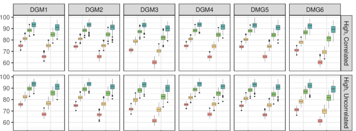
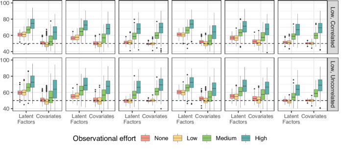
Figure 2: Predictive Performance in Simulations. The methods considered use latent factors or observed covariates (horizontal axis). The method using latent factors is the proposed approach. The columns represent the 6 DGMs in Table 1. The rows correspond to combinations of the high and low signal scenarios and the two correlation values. Results are shown by observational effort for pairs of species by color.

First, we notice that the performance of both methods improves with higher observational effort, implying that both models accommodate that an unrecorded interaction that was possible to be recorded across many studies is most likely not possible. Therefore, focusing on pairs of species on the lower end of observational effort compares the model structure more directly. Across all 24 scenarios considered and across the spectrum of observational effort, our approach that uses latent factors performs better than or comparably to the method that uses covariates directly, and all alternatives considered in the supplement. The improvement by using the latent factors is most visible for the low observational effort pairs. The performance of our approach is essentially unaltered by whether the same or different covariates drive the different submodels, irrespective of whether these covariates are measured or correlated (DGM 1 vs 4, 2 vs 5, and 3 vs 6). Also, its performance is very similar when the covariates are correlated or not (comparing rows 1-2, and 3-4). The only exception is in the low information setting when all important covariates are unmeasured (rows 3 and 4, DGM 3 and 6), in which case correlation among covariates might improve the performance of the latent factor model. When the important covariates are measured, the performance of our model improves (comparing DGMs 1 through 3, and 4 through 6), though in the high information setting the model can learn interaction profiles even when the important covariates are all unmeasured and uncorrelated with the measured ones (DGM6, High, Uncorrelated). These results inform us that the latent factor model performs better than using covariates directly across a variety of scenarios, and agrees with prior work on this topic which illustrated that flexible approaches perform better than including the traits directly into the model (Pichler et al., 2020).

5.4   Results from additional simulation studies

Here, we summarize some additional simulation results, all of which are shown in the Supplement. We have found that our approach performs better (or equally as well) compared to all other approaches considered. In all scenarios, approaches that ignore the taxonomic and geographical biases lead to very poor performance for predicting missing interactions which deteriorates for species with a higher observational effort, and a smaller number of predicted possible interactions compared to their counterparts with bias correction (also noted by Weinstein & Graham (2017) and Graham & Weinstein (2018)). Using a higher number of latent factors $H$ with sufficient shrinkage, and incorporating the variance parameters $\tau$ improve the performance of the proposed approach. Cutting the feedback among the submodels for informing the latent factors performed better only in sparse settings and for pairs of species with high observational effort, indicating that the measured interactions can be helpful in informing the latent factors for predicting missing interactions.

We also found that the variable importance metric introduced in Section 4 accurately identifies the covariates that are important for forming interactions, without specifying the functional form in which covariates drive interactivity. We find that variable importance should be interpreted separately for continuous and binary covariates. Our approach to variable importance is based on resampling techniques, and as a result it is arguably not-fully Bayesian. As an alternative we investigated variable importance for the model that includes covariates and latent factors. Apart from requiring a parametric specification of how covariates are included in the model, we find that using the coefficients of the covariates from this model for variable importance is flawed. This issue is related to spatial confounding in the spatial literature and arises due to collinearity of the phylogenetically-correlated covariates and latent factors (see Van Ee et al., 2022, for a discussion on spatial confounding in ecology, and references therein).

Across our simulations, we found that 1,000 MCMC iterations took on average 89 minutes. In the supplement, we also investigate the computational time of the proposed approach when varying the number of species and number of individual studies.

6.   Bird–plant interactions in the Atlantic Forest

We considered the two approaches that correct for taxonomic and geographic bias discussed in Section 5, and we use the increasing shrinkage prior on the latent factor coefficients. We specify $O_{ijs}=O_{is}^{B}O_{js}^{P}$, where $\bm{O}^{B}$ is an $n_{B}\times S$ binary occurrence matrix for birds, and similarly for $\bm{O}^{P}$. These are assumed known with entries equal to 1 if the species has a recorded interaction in the study and 0 otherwise. Due to a large number of recorded interactions with missing coordinate information, we are unable to include environmental or geographical covariates, though we discuss extensions in that direction in Supplement B.2. We ran four chains of 80,000 iterations each, with a 40,000 burn in, and kept every 40^th iteration. For our approach, 1,000 iterations took on average 86 minutes. MCMC convergence was investigated by studying traceplots and running means for identifiable parameters. Convergence diagnostics are shown in Supplement I. Based on similar diagnostics, we found that the MCMC of the alternative approach failed to converge based on the same number of iterations. For that reason, we excluded from this analysis the two traits of the plant species with the largest amounts of missingness (seed length and whether the species is threatened for extinction) which led to no detectable lack of convergence.

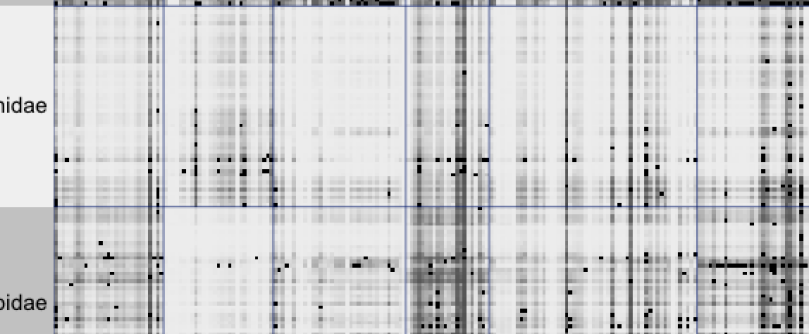
(a) Latent, Bias corrected

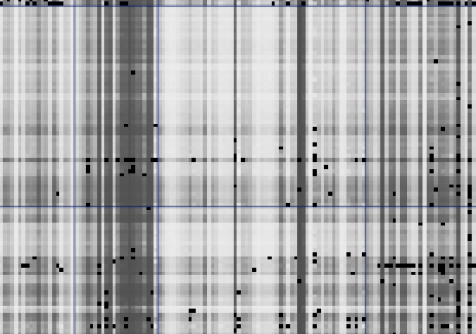
(b) Covariates, Bias corrected

Figure 3: Posterior Probability of Interactions. Posterior probability that bird species (y-axis) and plant species (x-axis) interact according to (a) the proposed method and (b) the alternative method. Species are organized in taxonomic families separated by blue lines. Only taxonomic families with at least 10 bird and 20 plant species are shown to ease visualization. Black color is used to represent recorded interactions.

In Figure 3, we show estimates for the probability of interaction for species in the largest taxonomic families. According to our model (Figure 3a), species in the same family form similar interactions as evidenced by the taxonomically-structured posterior interaction probabilities where the blue lines separate them in clusters with similar values. In contrast, results from the alternative approach that employs covariates directly (Figure 3b) indicate that some species interact with most other species and some species with none, as evidenced by rows and columns that are mostly close to one or zero. Since we do not expect this “all or none” structure in species interactions, results from the covariate approach seem untrustworthy, and indicate that it might rely on covariates too heavily. Species within the same family can belong to different genera, though genera are not shown in the figure to ease visualization. However, we observed that clusters of posterior interaction probabilities from the latent factor model within the depicted taxonomic families generally correspond to species organization by genera, supporting that interactions are taxonomically structured. The taxonomic structure is further supported by posterior means (95% credible intervals) for $\rho_{U}$ and $\rho_{V}$ which were 0.97 $(0.947,0.988)$ and 0.95 $(0.935,0.97)$, respectively. In Supplement H we show that the results remain unchanged when using an alternative specification of the intra-species correlation matrix based on species’ taxonomic relationships.

6.1   Comparison of model results and performance

The two approaches often return opposite conclusions about species’ interactions. The latent factor approach almost always returns probabilities of interaction that are lower than those from the covariate approach. The covariate approach predicts that 18% of pairs interact (posterior probability above 80%), and only 9% of pairs do not (posterior probability below 10%), both unrealistic. In contrast, the latent factor model predicts that 5% of pairs interact, and 41% do not. The vast majority of pairs that are predicted to not interact under the covariate model are also predicted to not interact based on the latent factor model, though the latent factor approach has substantially lower posterior standard deviation in these predictions. A more in-depth comparison is given in Supplement H.

To compare model performance directly, we applied a variant of cross-validation. We randomly choose 100 recorded interactions, we set their corresponding values in the observed interaction matrix equal to 0, and we predict their probability of interaction. We repeat this procedure 30 times, each time holding out a different subset of recorded interactions. Our setting forbids us from comparing model performance based on unrecorded interactions, since those interactions are not certainly impossible. Our comparison is based on how well each approach can differentiate the held-out pairs of species that truly interact from the group of all pairs, which necessarily includes pairs that do not interact. Since the two approaches return drastically different prevalence of interactions, we evaluate the relative magnitude of posterior interaction probabilities in the held-out and in the overall data. For the covariate approach, the mean and median posterior probability of interaction for the held out pairs was on average 1.21 and 1.36 times higher than the corresponding value across all pairs of species. In contrast, those numbers where substantially higher and equal to 1.85 and 3.19 for the mean and median, respectively, for our approach. Therefore, our approach is much more effective in differentiating the pairs that are truly interactive from the set of all pairs compared to the approach that uses covariates directly.

6.2   The importance of traits and phylogeny for species interactivity

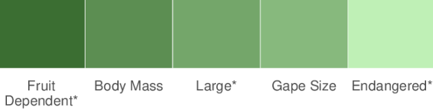
(a) Bird Traits Importance

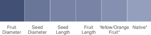
(b) Plant Traits Importance

(c) Interaction matrix ordered by traits

Figure 4: Figures (a) and (b) show the variable importance metric of Section 4 for bird and plant species, which should be interpreted separately for continuous and binary traits. Traits are ordered from most important (dark color) to least important (light color), and ^∗ is used for binary traits. Figure (c) shows the matrix of posterior probabilities of interaction where the species are re-ordered in increasing order of body mass for birds and fruit diameter for plants. Pink and green are used for low and high probability of interaction, respectively, and dark green is used for recorded interactions.

Apart from understanding which pairs of species are interactive, ecologists are also interested in understanding the traits which make species interactions possible (Garrard et al., 2013; Bastazini et al., 2017; Troscianko et al., 2017). Figures 4(a-b) show the variable importance metric described in Section 4 for bird and plant traits. We identify a bird’s body mass and a plant’s fruit diameter as the most important continuous traits in forming interactions. In Figure 4(c) we plot the posterior probabilities of interaction reordering the species in increasing values of the two covariates. High posterior probabilities are concentrated on the upper left triangle, indicating that a given bird would interact with most plant species that are smaller than some threshold size, in line with the current ecological literature (Fenster et al., 2015). At the same time, there seems to be some preference for larger birds to not consume fruits that are too small, indicating a matching-size type of behavior for forming interactions. These results illustrate that our approach can identify complicated interactive relationships without having to specify these trends parametrically.

We studied the overall importance of these traits and phylogenetic information using the cross-validation technique discussed in Section 6.1. For trait importance, we excluded each of the traits from the available information, separately, and for the phylogenetic information we set $\rho_{U},\rho_{V}$ to 0 which forces the latent factors to not be phylogenetically structured a priori. Excluding bird mass or fruit diameter returned on average a median posterior probability of interaction for the held out pairs 3.17 and 3.06 times higher, respectively, than the corresponding value across all pairs, compared to 3.19 when all traits are included. Therefore, fruit diameter can be an important covariate to measure for predicting species interactions. When ignoring phylogenetic information the corresponding value was 1.66 illustrating that phylogenetic information is crucial for predicting missing interactions.

7.   Discussion

We introduced an approach based on latent factors that uses species traits and recorded interactions to complete the bipartite graph of species interdependence accounting for the taxonomic and geographic biases of individual studies, and we proposed an approach to study variable importance in latent network models. We found that using covariates to inform the latent factors performs better in predicting pairs of species that do not interact and separating those that interact from the rest, compared to using the covariates directly. Even though using the covariates in the proposed manner complicates the investigation of variable importance, we proposed a variable importance metric which performed well in simulations and identified important physical traits for species interdependence that are in line with ecological knowledge.

A possible extension to our model could accommodate simultaneous modeling of species co-occurrence, that would allow us to incorporate geographic information and other environmental variables that define the environmental niche of the species such as temperature, precipitation, and evapotraspiration (Gravel et al., 2019). Even though we provide an overview of such an approach in the supplement, studying the co-existence of species across space is a hard problem in itself and it is the topic of joint species distribution modeling in ecology (Ovaskainen & Abrego, 2020). Importantly, modeling species co-occurrence and interactivity simultaneously and allowing for different interaction profiles based on environmental and geographical covariates would open the road to investigating the importance of species abundance, co-occurrence and competition in forming interactions. We find this to be an exciting line of future work.

Supplementary materials for
Covariate-informed latent interaction models: Addressing geographic & taxonomic bias in predicting bird-plant interactions
by
Georgia Papadogeorgou, Carolina Bello, Otso Ovaskainen, David B. Dunson

Appendix A Notation

Table S.1: Glossary of notation.

$n_{B},n_{P},S$	Number of bird species, plant species, and ecological studies, respectively.
$i,j,s$	Index for bird species, plant species, and study, respectively.
$p_{B},p_{P}$	Number of measured traits for bird and plant species, respectively.
$\bm{X}_{i}$, $\bm{W}_{j}$	Vectors of length $p_{B}$ and $p_{P}$ including the measured covariates of bird $i$ and plant $j$, respectively.
$\bm{X}_{.k}$	Vector of length $n_{B}$ including the entries of the $k^{th}$ measured bird trait.
$p_{i},q_{j}$	Detectability score for bird $i$ and plant $j$, respectively. Values in (0, 1).
$\bm{A},\bm{F},\bm{O}$	Arrays of dimension $n_{B}\times n_{P}\times S$ with binary entries. Entry $A_{ijs}$ is equal to 1 if study $s$ recorded an interaction between bird $i$ and plant $j$, and 0 otherwise. Entry $F_{ijs}$ reflects whether species $i,j$ were part of the taxonomic focus of study $s$, it is equal to 1 if study $s$ would have recorded the $ij$ interaction if observed, and 0 otherwise. Entry $O_{ijs}$ is equal to 1 if species $i,j$ co-exist in the geographical area covered by study $s$, and 0 otherwise.
$\bm{L}$	Matrix of dimension $n_{B}\times n_{P}$ with binary entries. Entry $L_{ij}$ is equal to 1 if bird $i$ is possible to interact with plant $j$ if given the opportunity.
$l_{ij}^{(r)},\bm{l}_{.j}^{(r)}$	Logit of the probability of interaction from Equation 5 for pair $ij$ at the $r^{th}$ MCMC iteration, and vector of length $n_{B}$ including the $l_{ij}^{(r)}$ values for all $i$.
$H$	Number of latent factors for both bird and plant species.
$\bm{U}_{i},\bm{V}_{j}$	Vector of length $H$ including bird $i$’s and plant $j$’s latent factors, respectively.
$\beta_{m0},\bm{\beta}_{m}$	Intercept and vector of length $H$ including the coefficients of the $H$ bird latent factors in the regression model of bird species’ $m^{th}$ measured trait.
$\gamma_{l0},\bm{\gamma}_{l}$	Same as above for the plant species and their $l^{th}$ measured trait.
$\lambda_{0},\lambda_{h}$	Parameters in the interaction submodel, intercept and coefficient of the product of the $h^{th}$ latent factors.
$\delta_{0},\bm{\delta}$	Intercept and coefficients of the $H$ bird latent factors in the bird detectability submodel.
$\zeta_{0},\bm{\zeta}$	Same as above for the plant detectability submodel.
$\sigma^{2}_{p,B},\sigma^{2}_{q,P}$	Residual variance for the detectability submodels for bird and plant species, respectively.
$\Sigma_{U},\Sigma_{V}$	Covariance matrix for the bird and plant latent factors of dimensions $n_{B}\times n_{B}$ and $n_{P}\times n_{P}$, respectively.
$\bm{C}_{U},\bm{C}_{V}$	Phylogenetic correlation matrices for bird and plant species, respectively.
$\rho_{U},\rho_{V}$	Parameters in (0, 1) for bird and plant species, respectively, deciding how much weight to give to phylogentic correlation matrix and the identity matrix in the definition of $\Sigma_{U},\Sigma_{V}$.
$\theta,\tau$	Global and parameter-specific variance terms in the increasing shrinkage prior used for the coefficients of the latent factors in the various submodels.
$\pi$, $\omega$, $v$, $\alpha$, $\alpha_{\theta}$, $\beta_{\theta}$, $\theta_{\infty}$	Additional parameters of the increasing shrinkage prior.

Below we introduce some additional notation that is used throughout the Supplement.

1. Outer product: We use $\bm{A}\otimes\bm{B}$ to denote the outer product of vector $\bm{A}$ of length $l_{A}$ and vector $\bm{B}$ of length $l_{B}$, where $\bm{A}\otimes\bm{B}$ is a matrix of dimension $l_{A}\times l_{B}$ with $(i_{1},i_{2})$ entry equal to $A_{i_{1}}B_{i_{2}}$.

2. Vectorization: For a matrix $\bm{M}$ of dimension $r\times c$, denote the vectorization of $\bm{M}$ as $\text{vec}(\bm{M})$ where $\text{vec}(\bm{M})$ is a vector of length $rc$ with entries

   $$M_{11},M_{12},\dots,M_{1c},M_{21},\dots,M_{2c},\dots,M_{rc},$$

   hence unpacking first across the columns and then across the rows.

3. Conditional distributions: We use $p(x_{1}\mid x_{2},x_{3})$ to denote the distribution of $x_{1}$ given $x_{2}$ and $x_{3}$, $p(x\mid\cdot)$ to denote the distribution of $x$ given everything else, and $p(x\mid\cdot,-y)$ to denote the distribution of $x$ given everything except $y$.

4. We often deal with matrices of dimension $n_{B}\times n_{P}$ (such as $\bm{L}$) or with 3-dimensional arrays with dimension $n_{B}\times n_{P}\times S$ (such as $\bm{A}$). We always denote the entries corresponding to bird species by $i$, to plant species with $j$, and studies with $s$. So an entry in $\bm{A}$ is $A_{ijs}$ and an entry in $\bm{L}$ is $L_{ij}$.

   To avoid heavy notation, in what follows, we use $\{L\}=\{L_{ij}\}_{i,j}$ to denote the collection of all elements in $\bm{L}$ across all indices $i$ and $j$, $\{L_{i}\}=\{L_{ij}\}_{j}$ to denote the collection of elements in $\bm{L}$ corresponding to bird index $i$ only and all indices $j$, $\{A_{s}\}=\{A_{ijs}\}_{i,j}$ to denote all elements in $\bm{A}$ corresponding to study $s$, $\{\bm{X}\}$ the collection of covariates for all bird species, etc.

Appendix B Observed data likelihood

Our observed data include the measured networks across studies $\bm{A}$, and the measured covariate information $\bm{X},\bm{W}$. We also know the focus of each study $\bm{F}$. We would like to acquire a model for the observed data corresponding to the measured networks and measured covariate values conditional on the studies’ focus, $P(\{A\},\{\bm{X}\},\{\bm{W}\}\mid\{F\})$.

B.1   Conditional distribution of measured networks

We first focus on the likelihood of the measured networks conditional on covariates, $P(\{A\}\mid\{\bm{X}\},\{\bm{W}\},\{F\})$. We believe that correlations across $A_{ijs}$ for different values of $i,j,s$ can arise due to the following reasons:

1. Studies that are geographically close are more likely to record similar interactions since the same species might co-occurring in both study areas. Conditioning on species co-occurrence should account for this type of dependence.

2. Species-oriented studies that focus on the same species will exhibit correlated records of interactions. Conditioning on the study’s focus should account for this type of dependence.

3. If an interaction is truly impossible, it will induce correlation across records, since none of the studies will record the specific interaction. Conditioning on the true interaction indicator should account for this type of dependence in the measured networks.

4. Species that have similar covariate profiles (either observed covariates or latent features) might exhibit similar profiles for which interactions are possible, and might have related co-occurrence patterns. Conditioning on the true interaction indicators and the occurrence of the species should account for this type of dependence as well.

5. Species that are hard to detect because of their behavior or physical characteristics will be hard to detect across studies, and their records of interactions will be correlated across studies. Conditioning on the probability of detecting a species should account for this type of dependence.

To summarize the points above, we assume that, conditional on studies’ focus, species occurrence across study sites, the true matrix of possible interactions, and species detectability, the records of interactions are independent across studies and across pairs of species, and they no longer depend on their measured or latent covariates. Therefore, for $a_{ijs}\in\{0,1\}$ representing a possible realization of the $(i,j)$ interaction in the $s^{th}$ measured networks and $\{a\}$ representing its collection across $i,j$ and $s$, we can write the recorded networks’ conditional likelihood as

$$P \left(\{A\}=\{a\}\mid\{\bm{X}\},\{\bm{W}\},\{\bm{U}\},\{\bm{V}\},\{L\},\{F\},\{O\},\{p\},\{q\}\right)=$$ (S.1)

$$=P\left(\{A\}=\{a\}\mid\{L\},\{F\},\{O\},\{p\},\{q\}\right)$$

$$=\prod_{i,j,s}P\left(A_{ijs}=a_{ijs}\mid\{L\},\{F\},\{O\},\{p\},\{q\}\right)$$

$$=\prod_{i,j,s}P\left(A_{ijs}=a_{ijs}\mid L_{ij},F_{ijs},O_{ijs},p_{i},q_{j}\right),$$

where the first and second equality stem from the conditional independence assumptions described above, and the third equality stems from a type of “individuality” assumption that the only study focus, species occurrence, and the possibility of an interaction that matter are those that involve the given pair and the specific study.

In Equation S.1, we have one term for each $(i,j,s)$ combination. The $(i,j,s)$ triplets can be split into two groups: those for which $F_{ijs}O_{ijs}L_{ij}=1$ and an interaction between the species in the given pair in the specific study is possible to be recorded, and those for which $F_{ijs}O_{ijs}L_{ij}=0$ and an interaction is impossible to be recorded. Therefore, Equation S.1 can be re-written as

$$\prod_{\begin{subarray}{c}{i,j,s}\\ F_{ijs}O_{ijs}L_{ij}=1\end{subarray}}P\left(A_{ijs}=a_{ijs}\mid L_{ij},F_{ijs},O_{ijs},p_{i},q_{j}\right)\prod_{\begin{subarray}{c}{i,j,s}\\ F_{ijs}O_{ijs}L_{ij}=0\end{subarray}}P\left(A_{ijs}=a_{ijs}\mid L_{ij},F_{ijs},O_{ijs},p_{i},q_{j}\right)$$

$$=\prod_{\begin{subarray}{c}{i,j,s}\\ F_{ijs}O_{ijs}L_{ij}=1\end{subarray}}(p_{i}q_{j})^{a_{ijs}}(1-p_{i}q_{j})^{1-a_{ijs}}\prod_{\begin{subarray}{c}{i,j,s}\\ F_{ijs}O_{ijs}L_{ij}=0\end{subarray}}I\left(a_{ijs}=0\right).$$

For the first term, it is assumed that a study will record a possible interaction with probability that is equal to the product of the individual species detectability probabilities ($p_{i}q_{j}$). For the second term, since the study could not have recorded the given interaction, the only allowed value for whether the interaction is recorded is $a_{ijs}=0$.

B.2   Distribution of latent parameters

To go from the distribution in Equation S.1 to $P(\{A\}=\{a\}\mid\{\bm{X}\},\{\bm{W}\},\{F\})$ one would need to integrate over the distribution of

$$p \left(\{\bm{U}\},\{\bm{V}\},\{O\},\{L\},\{p\},\{q\}\mid\{\bm{X}\},\{\bm{W}\},\{F\}\right)=$$

$$=p\left(\{q\}\mid\{\bm{U}\},\{\bm{V}\},\{O\},\{L\},\{p\},\{\bm{X}\},\{\bm{W}\},\{F\}\right)$$

$$\hskip 20.0ptp\left(\{p\}\mid\{\bm{U}\},\{\bm{V}\},\{O\},\{L\},\{\bm{X}\},\{\bm{W}\},\{F\}\right)$$

$$\hskip 20.0ptp\left(\{L\}\mid\{\bm{U}\},\{\bm{V}\},\{O\},\{\bm{X}\},\{\bm{W}\},\{F\}\right)$$

$$\hskip 20.0ptp\left(\{O\}\mid\{\bm{U}\},\{\bm{V}\},\{\bm{X}\},\{\bm{W}\},\{F\}\right)$$

$$\hskip 20.0ptp\left(\{\bm{U}\},\{\bm{V}\}\mid\{\bm{X}\},\{\bm{W}\},\{F\}\right)$$

$$=\Big{\{}\prod_{j}p\left(q_{j}\mid\bm{V}_{j},\bm{W}_{j}\right)\Big{\}}\Big{\{}\prod_{i}p\left(p_{i}\mid\bm{U}_{i},\bm{X}_{i}\right)\Big{\}}\Big{\{}\prod_{i,j}p\left(L_{ij}\mid\bm{U}_{i},\bm{V}_{j},\bm{X}_{i},\bm{W}_{j}\right)\Big{\}}{}$$ (S.2)

$$\hskip 20.0pt\Big{\{}\prod_{i,s}p(O^{B}_{is})\Big{\}}\Big{\{}\prod_{j,s}p(O^{P}_{js})\Big{\}}p\left(\{\bm{U}\},\{\bm{V}\}\mid\{\bm{X}\},\{\bm{W}\},\{F\}\right).$$

The last equation holds because we assume that (1) species detectability depends on their individual characteristics (measured or latent), is independent across species, and does not depend on species co-occurrence or study focus, (2) whether an interaction is possible depends solely on the covariates of the species involved, is independent across pairs, and does not depend on species co-occurrence which essentially limits the possibility of competition among species, and (3) we have access to the probability that species occur in a study area, so $O_{is}^{B},O_{js}^{P}$ are probabilistic draws from this distribution and they do not depend on remaining information.

Note on species co-occurrence and environmental covariates

A future direction could combine modeling of possible interactions with modeling species co-occurrence, a hard problem in its own right. In that situation, one could specify in the equality above that

$$p \left(\{O\}\mid\{\bm{U}\},\{\bm{V}\},\{L\},\{\bm{X}\},\{\bm{W}\},\{F\}\right)$$

$$=\Big{\{}\prod_{i,s}p\left(O_{is}^{B}\mid\bm{U}_{i},\bm{X}_{i},\{L_{i}\},\{O_{s}^{P}\}\right)\Big{\}}\Big{\{}\prod_{j,s}p\left(O_{js}^{P}\mid\bm{V}_{i},\bm{W}_{i},\{L_{j}\}\right)\Big{\}}.$$

This would entail an assumption that a species’ occurrence depends on its individual characteristics, and the set of species it can interact with, and the species of the other set that occur in each study area. To satisfy this assumption or to improve precision of these models, one might also include environmental covariates in the occurrence models, such as altitude, temperature and precipitation. Such covariates are believed to influence species co-occurrence more than whether species truly interact (Gravel et al. 2019), so they would be most useful to be included when species co-occurrence is modeled than when considered known.

B.3   Distribution of measured and latent covariates

The last term in the distribution for all latent variables correspond to the conditional distribution of latent covariates given measured covariates and the studies’ focus. This term is combined with the likelihood for the covariates and we write

$$p \left(\{\bm{U}\},\{\bm{V}\}\mid\{\bm{X}\},\{\bm{W}\},\{F\}\right)p\left(\{\bm{X}\},\{\bm{W}\}\mid\{F\}\right)$$

$$=p\left(\{\bm{X}\},\{\bm{W}\}\mid\{\bm{U}\},\{\bm{V}\},\{F\}\right)p\left(\{\bm{U}\},\{\bm{V}\}\mid\{F\}\right)$$

$$=p\left(\{\bm{X}\},\{\bm{W}\}\mid\{\bm{U}\},\{\bm{V}\}\right)p\left(\{\bm{U}\},\{\bm{V}\}\right)$$

$$=\Big{\{}\prod_{i}p(\bm{X}_{i}\mid\bm{U}_{i})\Big{\}}\Big{\{}\prod_{j}p(\bm{W}_{j}\mid\bm{V}_{j})\Big{\}}p(\{\bm{U}\})p(\{\bm{V}\}).$$

This representation holds because we assume that studies’ focus is not related to species’ measured or latent covariates, and that a species’ latent or measured covariates are not informative of another species’ covariates.

B.4   Using the same latent covariates in all the models

In Equation S.2 we see that the measured and latent covariates co-exist in the detection and interaction submodels. In their most generality, the latent covariates ($\bm{U}$ for bird species and $\bm{V}$ for plant species) can be arbitrarily close to the measured covariates ($\bm{X}$ for bird species and $\bm{W}$ for plant species). If the latent covariates capture the information in the measured covariates sufficiently well, then the measured covariates can be excluded from the detectability and interaction submodels in Equation S.2, and we could allow

$$p\left(q_{j}\mid\bm{V}_{j},\bm{W}_{j}\right) =p\left(q_{j}\mid\bm{V}_{j}\right)$$

$$p\left(p_{i}\mid\bm{U}_{i},\bm{X}_{i}\right) =p\left(p_{i}\mid\bm{U}_{i}\right),\quad\text{and}$$

$$p\left(L_{ij}\mid\bm{U}_{i},\bm{V}_{j},\bm{X}_{i},\bm{W}_{j}\right) =p\left(L_{ij}\mid\bm{U}_{i},\bm{V}_{j}\right).$$

In addition, the latent covariates could be allowed to be higher-dimensional than the measured covariates capturing different features of the species that are not immediately available in the measured covariates. These features could be informative in one of the submodels without necessarily being informative in the others. For example, one of the variables in $\bm{U}$ can be informative for detectability and not informative for forming interactions. This covariate could still be included in the interaction submodel without creating any issues. Therefore, if latent features are sufficiently high-dimensional and resemble the measured covariates, we can allow all latent features to be included in each model component and measured covariates would no longer be directly necessary.

B.5   Distribution of measured and latent variables

Measured variables correspond to the measured networks and measured covariate information for the species. Latent variables correspond to every other variable discussed above: latent covariate information, detectability probabilities, the true interaction matrix, and the occurrence indicators. Combining the discussion above, we have the joint distribution of all these variables as

$$p \left(\{A\}=\{a\},\{\bm{X}\},\{\bm{W}\},\{\bm{U}\},\{\bm{V}\},\{L\},\{O\},\{p\},\{q\}\mid\{F\}\right)=$$

$$=\Big{\{}\prod_{\begin{subarray}{c}{i,j,s}\\ F_{ijs}O_{ijs}L_{ij}=1\end{subarray}}(p_{i}q_{j})^{a_{ijs}}(1-p_{i}q_{j})^{1-a_{ijs}}\Big{\}}\Big{\{}\prod_{\begin{subarray}{c}{i,j,s}\\ F_{ijs}O_{ijs}L_{ij}=0\end{subarray}}I\left(a_{ijs}=0\right)\Big{\}}\times$$

$$\hskip 20.0pt\Big{\{}\prod_{i}p\left(p_{i}\mid\bm{U}_{i}\right)\Big{\}}\Big{\{}\prod_{j}p\left(q_{j}\mid\bm{V}_{j}\right)\Big{\}}\Big{\{}\prod_{i,j}p\left(L_{ij}\mid\bm{U}_{i},\bm{V}_{j}\right)\Big{\}}\Big{\{}\prod_{i,s}p(O^{B}_{is})\Big{\}}\Big{\{}\prod_{j,s}p(O^{P}_{js})\Big{\}}\times$$

$$\hskip 20.0pt\Big{\{}\prod_{i}p(\bm{X}_{i}\mid\bm{U}_{i})\Big{\}}\Big{\{}\prod_{j}p(\bm{W}_{j}\mid\bm{V}_{j})\Big{\}}p(\{\bm{U}\})p(\{\bm{V}\})$$

Appendix C MCMC scheme

C.1   List of model parameters to be updated in an MCMC

Model parameters to be updated include

• the $(n_{B}\times n_{P})$ true interaction matrix $\bm{L}$,

• the parameters of the interaction model $\bm{\lambda}$ where $\bm{\lambda}=(\lambda_{1},\lambda_{2},\dots,\lambda_{H})^{T}$

• the latent factors $\bm{U},\bm{V}$ of dimension $(n_{B}\times H)$ and $(n_{P}\times H)$ respectively,

• the parameters of the trait models: $\bm{B}$ and $\bm{\Gamma}$, where $\bm{B}=(\bm{\beta}_{1}\ \bm{\beta}_{2}\ \dots\ \bm{\beta}_{p_{B}})$ is of dimension $H\times p_{B}$, and $\bm{\Gamma}=(\bm{\gamma}_{1}\ \bm{\gamma}_{2}\ \dots\ \bm{\gamma}_{p_{P}})$ is of dimension $H\times p_{P}$, and the residual variances $\sigma^{2}_{m}$ and $\sigma^{2}_{l}$ of continuous traits,

• the parameters of the models for the probability of observing a true interaction of a given species $\bm{\delta}$ and $\bm{\zeta}$ and the residual variances $\sigma^{2}_{p,B},\sigma^{2}_{q,P}$,

• the probabilities themselves $\bm{p}_{B}=(p_{1},p_{2},\dots,p_{n_{B}})$, and $\bm{q}_{P}=(q_{1},q_{2},\dots,q_{n_{P}})$,

• the matrices representing species occurrence across studies $\bm{O}^{B}\in\{0,1\}^{n_{B}\times S}$ and $\bm{O}^{B}\in\{0,1\}^{n_{P}\times S}$ based on which the array of co-occurrences $\bm{O}\in\{0,1\}^{n_{B}\times n_{P}\times S}$ is defined as $O_{ijs}=O^{B}_{is}O^{P}_{js}$,

• the parameter in the latent factor covariance matrices $\rho_{U},\rho_{V}$,

• the variance scaling parameters $\tau$ across all models,

• the parameters $\bm{\theta},\bm{\pi},\bm{\omega}$ and $\bm{v}$ controlling the increasing shrinkage prior, and

• covariate missing values, if applicable.

C.2   The posterior distribution

The posterior distribution of all model parameters (assuming no missing values of covariates) is

$$p(\text{parameters}\mid \text{Data})\propto$$

$$\propto\prod_{m=1}^{p_{B}}p(\bm{X}_{.m}\mid\bm{\beta}_{m.},\bm{U},\sigma^{2}_{m})\times\prod_{l=1}^{p_{P}}p(\bm{W}_{.l}\mid\bm{\gamma}_{l.},\bm{V},\sigma^{2}_{l})$$

$$\hskip 40.0pt\times\Big{\{}\prod_{s=1}^{S}\prod_{i=1}^{n_{B}}\prod_{j=1}^{n_{P}}p(A_{ijs}\mid p_{i},q_{j},L_{ij},F_{ijs},O_{ijs})\Big{\}}$$

$$\hskip 40.0pt\times\Big{\{}\prod_{i=1}^{n_{B}}\prod_{j=1}^{n_{P}}p(L_{ij}\mid\bm{\lambda},\bm{U}_{i.},\bm{V}_{j.})\Big{\}}$$

$$\hskip 40.0pt\times\Big{\{}\prod_{i=1}^{n_{B}}p(\text{logit}({p_{i}})\mid\bm{\delta},\bm{U}_{i.},\sigma^{2}_{p,B})\Big{\}}\times\Big{\{}\prod_{j=1}^{n_{P}}p(\text{logit}({q_{j}})\mid\bm{\zeta},\bm{V}_{j.},\sigma^{2}_{q,P})\Big{\}}$$

$$\hskip 40.0pt\times\prod_{h=1}^{H}\Big{\{}p(\bm{U}_{.h}\mid\bm{\Sigma}_{U})\ p(\bm{V}_{.h}\mid\bm{\Sigma}_{V})\Big{\}}$$

$$\hskip 40.0pt\times\Big{\{}\prod_{s=1}^{S}\prod_{i=1}^{n_{B}}\prod_{j=1}^{n_{P}}p(O_{ijs})\Big{\}}$$

$$\hskip 40.0pt\times p(\rho_{U})p(\rho_{V})$$

$$\hskip 40.0pt\times\prod_{m=1}^{p_{B}}p(\beta_{m0})\prod_{h=1}^{H}p(\beta_{mh}\mid\tau_{mh}^{\beta},\theta_{h})$$

$$\hskip 40.0pt\times\prod_{l=1}^{p_{P}}p(\gamma_{l0})\prod_{h=1}^{H}p(\gamma_{lh}\mid\tau_{lh}^{\gamma},\theta_{h})$$

$$\hskip 40.0pt\times p(\lambda_{0})p(\delta_{0})p(\zeta_{0})\prod_{h=1}^{H}p(\lambda_{h}\mid\tau_{h}^{\lambda},\theta_{h})p(\delta_{h}\mid\tau_{h}^{\delta},\theta_{h})p(\zeta_{h}\mid\tau_{h}^{\zeta},\theta_{h})$$

$$\hskip 40.0pt\times\prod_{h=1}^{H}\left[p(\tau_{h}^{\delta})p(\tau_{h}^{\zeta})p(\tau_{h}^{\lambda})\prod_{m=1}^{p_{B}}p(\tau_{mh}^{\beta})\prod_{l=1}^{p_{P}}p(\tau_{lh}^{\gamma})\right]$$

$$\hskip 40.0pt\times\prod_{h=1}^{H}p(\theta_{h}\mid\pi_{h})p(\pi_{h}\mid\omega_{1},\omega_{2},\dots,\omega_{h})p(\omega_{h}\mid v_{1},v_{2},\dots,v_{h})p(v_{h}),$$

where $p(\pi_{h}\mid\omega_{1},\omega_{2},\dots,\omega_{h})$ and $p(\omega_{h}\mid v_{1},v_{2},\dots,v_{h})$ are point mass distributions satisfying the equations in Equation 8.

C.3   MCMC updates

Updating the true interaction matrix $\bm{L}$

In deriving the posterior distribution of $L_{ij}$ we found that for pairs $(i,j)$ for which there exists a study $s$ that recorded their interaction, $A_{ijs}=1$, we have that $P(L_{ij}=1\mid\cdot)=1$. Therefore, if $A_{ijs}=1$ for at least one $s$, then $L_{ij}$ is set to 1. Now, in the case where the interaction is unrecorded across all studies, $A_{ijs}=0$ for all $s$, $L_{ij}$ is sampled using a Bernoulli distribution with

$$p(L_{ij}=l\mid\cdot)\propto\begin{cases}1-p_{ij}^{L},&\text{if }l=0\\ p_{ij}^{L}(1-p_{i}q_{j})^{\sum_{s}F_{ijs}O_{ijs}}&\text{if }l=1,\end{cases}$$

where $p_{ij}^{L}=\text{expit}\left\{\lambda_{0}+\sum_{h=1}^{H}\lambda_{h}U_{ih}V_{jh}\right\}$, and $p_{i},q_{j}$ are the probabilities of observing bird $i$ and plant $j$ in Equation 6. Notice that when $A_{ijs}=0$ for all $s$, the probability that the interaction is possible is smaller when $\sum_{s}F_{ijs}O_{ijs}$ is larger. This makes intuitive sense as are under the scenario where the interaction was not recorded across any study, and this quantity counts the number of studies for which the species $i,j$ co-occur, and the $(i,j)$ interaction would have been recorded if observed.

Updating the parameters $\bm{\lambda}$ of the interaction model

We update these parameters using the Pólya-Gamma data-augmentation of Polson et al. (2013) in the following manner:

1. For each $(i,j)$ pair, draw latent variables $\omega_{ij}^{L}\sim\text{PG}(1,\lambda_{0}+\sum_{h}\lambda_{h}U_{ih}V_{jh})$. Conditional on $\omega_{ij}^{L}$ the contribution of $L_{ij}$ to the likelihood is

   $$p(L_{ij}\mid\omega_{ij}^{L},\bm{\lambda},\bm{U}_{i.},\bm{V}_{j.})\propto\exp\left\{-\frac{\omega_{ij}^{L}}{2}\left[\frac{L_{ij}-1/2}{\omega_{ij}^{L}}-\left(\lambda_{0}+\sum_{h=1}^{H}\lambda_{h}U_{ih}V_{jh}\right)\right]^{2}\right\},$$

   which is the kernel of a normal distribution, and can be combined with the normal prior distribution on $\bm{\lambda}$.

2. Sample $\bm{\lambda}\sim N_{H+1}(\mu_{new},\bm{\Sigma}_{new})$ for parameters

   $$\bm{\Sigma}_{new}=\left[\bm{D}_{UV}^{T}\bm{\Omega}^{L}\bm{D}_{UV}+(\bm{\Sigma}_{0}^{\lambda})^{-1}\right]^{-1},$$

   and

   $$\mu_{new}=\bm{\Sigma}_{new}\left[\bm{D}_{UV}^{T}\left(\text{vec}(\bm{L})-1/2\right)+(\bm{\Sigma}_{0}^{\lambda})^{-1}\bm{\mu}_{0}^{\lambda}\right],$$

   where

   • $\bm{D}_{UV}$ is a matrix with $(n_{B}\times n_{P})$ rows and $(H+1)$ columns, with first column equal to 1, and $(h+1)^{th}$ column equal to

     $$\text{vec}(\bm{U}_{.h}\otimes\bm{V}_{.h})=(U_{1h}V_{1h},U_{1h}V_{2h},\dots,U_{1h}V_{n_{P}h},U_{2h}V_{1h},\dots,U_{2h}V_{n_{P}h},\dots,U_{n_{B}h}V_{n_{P}h}),$$

   • $\bm{\Omega}^{L}$ is a matrix of dimension $(n_{B}n_{P}\times n_{B}n_{P})$ with the entries $\text{vec}(\omega_{ij}^{L})$ on the diagonal and 0 everywhere else,

   • $\bm{\Sigma}_{0}^{\lambda}$ is a diagonal matrix with entries $\sigma_{0}^{2},\tau_{1}^{\lambda}\theta_{1},\tau_{2}^{\lambda}\theta_{h},\dots,\tau_{H}^{\lambda}\theta_{H}$ on the diagonal ($\sigma^{2}_{0}$ is the prior variance of $\lambda_{0}$), and

   • $\bm{\mu}_{0}^{\lambda}$ is equal to $(\mu_{0}^{\lambda_{0}},0,0,\dots,0)^{T}$, where $\mu_{0}^{\lambda_{0}}$ is the prior mean of $\lambda_{0}$.

Updating the variance scaling parameters $\tau$

Sample $\tau_{mh}^{\beta}$ from an inverse gamma distribution with parameters $(\nu+1)/2$ and $(\nu+\beta_{mh}^{2}/\theta_{h})/2$. Similarly for $\tau_{lh}^{\gamma},\tau_{h}^{\delta},\tau_{h}^{\zeta}$ and $\tau_{h}^{\lambda}$.

Updating the parameters of continuous traits models

For a continuous trait $m$, the full conditional posterior distribution of $\bm{\beta}_{m.}=(\beta_{m0},\beta_{m1},\dots,\beta_{mH})^{T}$ is $N_{H+1}(\bm{\mu}_{new},\bm{\Sigma}_{new})$ for parameters

$$\bm{\Sigma}_{new}=\left[\bm{D}_{B}^{T}\bm{D}_{B}/\sigma^{2}_{m}+(\bm{\Sigma}_{0}^{\beta})^{-1}\right]^{-1}$$

and

$$\bm{\mu}_{new}=\bm{\Sigma}_{new}\left[\bm{D}_{B}^{T}\bm{X}_{.m}/\sigma^{2}_{m}+(\bm{\Sigma}_{0}^{\beta})^{-1}\bm{\mu}_{0}^{\beta}\right],$$

where

• $\bm{D}_{B}=\left(\bm{1}\mid\bm{U}_{.1}\mid\bm{U}_{.2}\mid\dots\mid\bm{U}_{.H}\right)$ matrix of dimension $(n_{B}\times(H+1))$,

• $\bm{X}_{.m}$ vector of entries for the $m^{th}$ trait $(X_{1m},X_{2m},\dots X_{n_{B}m})^{T}$,

• $\bm{\Sigma}_{0}^{\beta}$ diagonal matrix with entries $\sigma^{2}_{0},\tau_{m1}^{\beta}\theta_{1},\dots,\tau_{mH}^{\beta}\theta_{H}$ ($\sigma^{2}_{0}$ is the prior variance of $\beta_{m0}$), and

• $\bm{\mu}_{0}^{\beta}=(\mu_{0}^{\beta_{0}},0,0,\dots,0)^{T}$ ($\mu_{0}^{\beta_{0}}$ is the prior mean of $\beta_{m0}$).

To update the residual variance of continuous trait $m$, we sample $\sigma^{2}_{m}$ from an inverse gamma distribution with parameters $a_{\sigma}+n_{B}/2$ and $b_{\sigma}+\sum_{i=1}^{n_{B}}(X_{im}-(1,\bm{U}_{i.}^{T})^{T}\bm{\beta}_{m.})^{2}/2$. Similarly we update parameters $\bm{\gamma}_{l.}=(\gamma_{l0},\gamma_{l1},\dots,\gamma_{lH})^{T}$ and $\sigma^{2}_{l}$ for continuous trait $\bm{L}$ of the other set of units.

Updating the parameters of binary traits models

To update the coefficients $\bm{\beta}_{m.}$ for a binary trait $m$ we again follow the Pólya-Gamma data augmentation approach. Specifically,

1. We sample $\omega_{im}$ from $\text{PG}(1,(1,\bm{U}_{i.}^{T})^{T}\bm{\beta}_{m.})$ for all $i=1,2,\dots,n_{B}$.

2. We draw $\bm{\beta}_{m.}$ from $N_{H+1}(\bm{\mu}_{new},\bm{\Sigma}_{new})$ for parameters

   $$\bm{\Sigma}_{new}=\left[\bm{D}_{B}^{T}\bm{\Omega}_{m}\bm{D}_{B}+(\bm{\Sigma}_{0}^{\beta})^{-1}\right]^{-1}$$

   and

   $$\bm{\mu}_{new}=\bm{\Sigma}_{new}\left[\bm{D}_{B}\left(\bm{X}_{.m}-1/2\right)+(\bm{\Sigma}_{0}^{\beta})^{-1}\bm{\mu}_{0}^{\beta}\right],$$

   where $\bm{\Sigma}_{0}^{\beta},\bm{\mu}_{0}^{\beta},\bm{D}_{B}$ and $\bm{X}_{.m}$ are as above, and $\Omega_{m}$ is a diagonal matrix with entries $\{\omega_{im}\}_{i=1}^{n_{B}}$.

Similarly we update the coefficients $\bm{\gamma}_{l.}=(\gamma_{l0},\gamma_{l1},\dots,\gamma_{lH})^{T}$ for the models of the binary traits for the other set of units.

Updating the parameters of the probability of observing an interaction

The parameters $\bm{\delta}$ and $\sigma^{2}_{p,B}$ are updated similarly to the updates for the parameters of the continuous trait models $\bm{\beta}$ and $\sigma^{2}_{m}$, using the same matrix $\bm{D}_{B}$, and setting

$$\bm{X}_{.m}=(\text{logit}({p_{1}}),\text{logit}({p_{2}}),\dots,\text{logit}({p_{n_{B}}}))^{T}.$$

The update of $\bm{\zeta}$ and $\sigma^{2}_{q,P}$ proceeds similarly.

Updating the latent factors

We describe the update of the latent factors for the first set of units $\bm{U}_{.h}$ for $h=1,2,\dots,H$, and updates for $\bm{V}_{.h}$ are similar. Here, we will use the Pólya-Gamma draws $\omega_{im}$ for binary traits $m$, and $\omega_{ij}^{L}$, described above. For each $h=1,2,\dots,H$, $\bm{U}_{.h}$ is drawn from $\mathcal{N}_{n_{B}}(\bm{\mu}_{new},\bm{\Sigma}_{new})$ for parameters

$$\bm{\Sigma}_{new}=\left(\sum_{\begin{subarray}{c}\text{m: }X_{m}\\ \text{continuous}\end{subarray}}\beta_{mh}^{2}/\sigma^{2}_{m}\bm{I}_{n_{B}}+\delta_{h}^{2}/\sigma^{2}_{p,B}\bm{I}_{n_{B}}+\sum_{\begin{subarray}{c}\text{m: }X_{m}\\ \text{binary}\end{subarray}}\beta_{mh}^{2}\bm{\Omega}_{m}+\sum_{j=1}^{n_{P}}\lambda_{h}^{2}V_{jh}^{2}\bm{\Omega}_{j}^{L}+\bm{\Sigma}_{U}^{-1}\right)^{-1}$$

and

$$\bm{\mu}_{new}=\bm{\Sigma}_{new}\Bigg{\{}\sum_{\begin{subarray}{c}\text{m: }X_{m}\\ \text{continuous}\end{subarray}} \beta_{mh}/\sigma^{2}_{m}\ \textbf{part}(m,h)+\delta_{h}/\sigma^{2}_{p,B}\ \textbf{part}(p,h)+$$

$$\sum_{\begin{subarray}{c}\text{m: }X_{m}\\ \text{binary}\end{subarray}}\beta_{mh}\bm{\Omega}_{m}\left[\left(\frac{\bm{X}-1/2}{\bm{\omega}}\right)_{m}-\left(1\mid\bm{U}_{.-h}\right)\bm{\beta}_{m(-h)}\right]+$$

$$\sum_{j=1}^{n_{P}}\lambda_{h}V_{jh}\bm{\Omega}_{j}^{L}\left[\left(\frac{\bm{L}-1/2}{\bm{\omega}}\right)_{j}-\left(1\mid\bm{U}_{.-h}\bm{V}_{j(-h)}\right)\bm{\lambda}_{-h}]\right]\Bigg{\}}$$

where

• $\bm{\Omega}_{j}^{L}$ is used to denote, with some abuse of notation, the diagonal matrix of dimension $n_{B}$ with entries representing the Pólya-Gamma draws from the interaction model involving unit $j$: $(\omega_{1j}^{L},\omega_{2j}^{L},\dots,\omega_{n_{B}j}^{L})$,

• $\bm{\Sigma}_{U}$ is the covariance matrix of the latent factors in the prior distribution specified in Section 3.3,

• $\textbf{part}(m,h)$ is used to denote the residuals from the model for $X_{m}$ when excluding the $h^{th}$ latent factor, and is the following vector of length $n_{B}$:

  $$\textbf{part}(m,h)=\bm{X}_{.m}-\big{(}\beta_{m0}\bm{1}+ \beta_{m1}\bm{U}_{.1}+\dots+\beta_{m(h-1)}\bm{U}_{.(h-1)}+$$

  $$\beta_{m(h+1)}\bm{U}_{.(h+1)}+\dots+\beta_{mH}\bm{U}_{.H}\big{)},$$

• Similarly, $\textbf{part}(p,h)$ is used to denote a vector of length $n_{B}$ including the residuals of the model for the probability of observing when excluding the $h^{th}$ latent factor:

  $$[\text{part}(p,h)]_{i}=\text{logit}({p_{i}})-\big{(}\delta_{0}+\delta_{1}U_{i1}+\dots+\delta_{h-1}U_{i(h-1)}+\delta_{h+1}U_{i(h+1)}+\dots+\delta_{H}U_{iH}\big{)},$$

• $\displaystyle\left(\frac{\bm{X}-1/2}{\bm{\omega}}\right)_{m}$ is a vector of length $n_{B}$ with $i^{th}$ element equal to $(X_{im}-1/2)/\omega_{im}$,

• $(1\mid\bm{U}_{.-h})$ is a matrix of dimension $n_{B}\times H$ representing a concatenation of a vector of 1 in the first column and the latent factors $\bm{U}$ excluding the $h^{th}$ one,

• $\bm{\beta}_{m(-h)}$ is the vector $\bm{\beta}_{m}$ excluding the coefficient of the $h^{th}$ latent factor,

• $\displaystyle\left(\frac{\bm{L}-1/2}{\bm{\omega}}\right)_{j}$ is the diagonal matrix of dimension $n_{B}$ including the transformed versions of unit $j$’s interactions: $\big{(}(L_{1j}-1/2)/\omega_{1j}^{L},(L_{2j}-1/2)/\omega_{2j}^{L},\dots,(L_{n_{B}j}-1/2)/\omega_{n_{B}j}^{L}\big{)}$,

• $\displaystyle\left(1\mid\bm{U}_{.-h}\bm{V}_{j(-h)}\right)$ is the $n_{B}\times H$ matrix with first column equal to 1, second column equal to $V_{j1}\bm{U}_{.1}=(U_{11}V_{j1},U_{21}V_{j1},\dots,U_{n_{B}1}V_{j1})^{T}$, third column equal to $V_{j2}\bm{U}_{.2}$, up to the last column which is equal to $V_{jH}\bm{U}_{.H}$, excluding the $h^{th}$ vector $V_{jh}\bm{U}_{.h}$, and always using the same unit $j$’s latent factors, and

• $\bm{\lambda}_{-h}$ includes the coefficients of the interaction model excluding $\lambda_{h}$.

Updating the parameters of the increasing shrinkage prior

In order to ease the updates of the increasing shrinkage prior parameters in Equation 8, we introduce parameters $z_{1},z_{2},\dots,z_{H}$ with $z_{h}\sim\text{Multinomial}(\omega_{1},\omega_{2},\dots,\omega_{H})$ and $\theta_{h}|z_{h}\sim I(z_{h}\leq h)\delta_{\theta_{\infty}}+I(z_{h}>h)P_{0}$, similarly to Legramanti et al. (2020). Then, updates of the parameters proceeds by updating the parameters $\{v_{h}\}_{h}$ which deterministically set the values of $\{\omega_{h}\}_{h}$ and $\{\pi_{h}\}_{h}$, and updating the parameters $\{z_{h}\}_{h}$ and $\{\theta_{h}\}_{h}$.

First, updates for $v_{h}$ are performed conditional on $z_{1},z_{2},\dots,z_{H}$ by counting the number of $z$’s with values equal or greater than $h$: $v_{h}$ is sampled from a Beta distribution with parameters $\left(1+\sum_{h^{\prime}=1}^{H}I(z_{h^{\prime}}=h),\alpha+\sum_{h^{\prime}=1}^{H}I(z_{h^{\prime}}>h)\right)$. Based on the sampled values for $v_{1},v_{2},\dots,v_{H}$, the values of $\omega_{h}$ are updated from their deterministic relationship in Equation 8.

Then, the variance parameters $\theta_{h}$ are updated using the part of the prior that is the slab $P_{0}$ or the spike $\delta_{\theta_{\infty}}$ depending on the value of the corresponding $z_{h}$:

• If $z_{h}\leq h$ (which happens with prior probability $\sum_{l=1}^{h}\omega_{l}=\pi_{h}$) the variance component $\theta_{h}$ belongs to the spike part of the prior, and it is set equal to $\theta_{\infty}$.

• If $z_{h}>h$, then $\theta_{h}$ belongs to the $P_{0}$ part of the prior which is an inverse gamma distribution in our case, and $\theta_{h}$ is drawn from an inverse gamma with parameters $\alpha_{\theta}+(p_{B}+p_{P}+3)/2$ and $\beta_{\theta}+\left(\sum_{m}\beta_{mh}^{2}/\tau_{mh}^{\beta}+\sum_{l}\gamma_{lh}^{2}/\tau_{lh}^{\gamma}+\lambda_{h}^{2}/\tau_{h}^{\lambda}+\delta_{h}^{2}/\tau_{h}^{\delta}+\zeta_{h}^{2}/\tau_{h}^{\zeta}\right)/2$.

Lastly, the parameters $z_{h}$ are updated from a Multinomial distribution such that

$$p(z_{h}=l\mid\cdot,-\bm{\theta})\propto\begin{cases}\omega_{l}\ \phi(\bm{x};\theta_{\infty}\bm{\Sigma})&\text{ for }l=1,2,\dots,h\\ \omega_{l}\ \tau(\bm{x};2\alpha_{\theta},\beta_{\theta}/\alpha_{\theta}\bm{\Sigma})&\text{ for }l=h+1,h+2,\dots,H,\end{cases}$$

where the vector $\bm{x}$ includes all coefficients of the $h^{th}$ latent factors: $\bm{x}=(\bm{\beta}_{.h}^{T},\bm{\gamma}_{.h}^{T},\lambda_{h},\delta_{h},\zeta_{h})^{T}$, $\bm{\Sigma}$ is a diagonal matrix with entries $\big{(}(\tau_{.h}^{\beta})^{T},(\tau_{.h}^{\gamma})^{T},\tau_{h}^{\lambda},\tau_{h}^{\delta},\tau_{h}^{\zeta}\big{)}$, $\phi(\bm{x};\theta_{\infty}\bm{\Sigma})$ is the density of a normal distribution centered at 0 with covariance matrix $\theta_{\infty}\bm{\Sigma}$ evaluated at $\bm{x}$, and $\tau(\bm{x};2\alpha_{\theta},\beta_{\theta}/\alpha_{\theta}\bm{\Sigma})$ is the density of a multivariate $t$-distribution with $2\alpha_{\theta}$ degrees of freedom and covariance matrix $\beta_{\theta}/\alpha_{\theta}\bm{\Sigma}$ evaluated at $\bm{x}$. Note here that, even though the covariance matrix is diagonal, the density of the multivariate $t$-distribution is not the same as the sum of the densities from univariate $t$-distributions.

Updating the probability of observing an interaction

Since the conditional posterior distributions of $p_{i}$, and $q_{j}$ are not of known distributional form, we update them using Metropolis-Hastings. To update $p_{i}$:

• If $p_{i}^{(t)}$ is the value of $p_{i}$ at iteration $t$, propose new value $x$ from Beta$(np_{i}^{(t)},n(1-p_{i}^{(t)}))$.

• Calculate the acceptance probability which is equal to

  $$AP =\left\{\prod_{j=1}^{n_{P}}\left[\frac{xq_{j}}{p_{i}^{(t)}q_{j}}\right]^{L_{ij}\sum_{s}(A_{ijs}F_{ijs}O_{ijs})}\left[\frac{1-xq_{j}}{1-p_{i}^{(t)}q_{j}}\right]^{L_{ij}\sum_{s}[(1-A_{ijs})F_{ijs}O_{ijs}]}\right\}$$

  $$\hskip 20.0pt\times\frac{\phi(\text{logit}({x});(1\ U_{i}^{T})\bm{\delta},\sigma^{2}_{p,B})}{\phi(\text{logit}({p_{i}^{(t)}});(1\ U_{i}^{T})\bm{\delta},\sigma^{2}_{p,B})}\times\frac{b(p_{i}^{(t)};nx,n(1-x))}{b(x;np_{i}^{(t)},n(1-p_{i}^{(t)}))},$$

  where all other parameters are set to their most recent values, and $b(x;a,b)$ is the density of a Beta$(a,b)$ distribution evaluated at x.

• Accept $x$ with probability $AP$, or stay at $p_{i}^{(t)}$ with probability $1-AP$.

Similarly update the parameters $q_{j}$.

Updating the indicator of species occurrence in a study area

We assume that the entries in $\bm{O}^{B}$ are a priori independent, and we specify that each entry arises from a Bernoulli random variable with probability of success $\pi_{O^{B}_{is}}$, pre-specified. When deriving the conditional posterior distribution of $O^{B}_{is}$ we find that if $A_{ijs}=1$ for some $j$, then $p(O^{B}_{is}=1\mid\cdot)=1$. This makes sense since $A_{ijs}=1$ for some $j$ means that study $s$ recorded an interaction of species $i$, which necessarily implies that the species exists in the area. Now, if $A_{ijs}=0$ for all $j$, then $O^{B}_{is}$ is drawn from a Bernoulli distribution with

$$p(O^{B}_{is}=o\mid\cdot)\propto\begin{cases}\pi_{O^{B}_{is}}\prod_{j=1}^{n_{P}}(1-p_{i}q_{j})^{L_{ij}F_{ijs}}&\text{if }o=1,\text{ and}\\ 1-\pi_{O^{B}_{is}},&\text{if }o=0.\end{cases}$$

This formula also makes intuitive sense. Essentially, if there are many species $j$ with which $i$ interacts and for which study $s$ could have observed an interaction, observing no interactions of $i$ must mean that the species do not occur.

Updating the latent factor covariance parameter

We update the parameters $\rho_{U},\rho_{V}$ using a Metropolis-Hastings step (similarly to the probability of detecting species). Specifically:

• If $\rho_{U}^{(t)}$ is the value of $\rho_{U}$ at iteration $t$, propose new value $x$ from Beta$(n\rho_{U}^{(t)},n(1-\rho_{U}^{(t)}))$.

• Calculate the current and proposed value for the correlation matrix and denote them by $\bm{\Sigma}_{U}^{(t)}$ and $\bm{\Sigma}_{U}^{x}$, respectively.

• Calculate the acceptance probability which is equal to

  $$AP=\frac{\prod_{h=1}^{H}\phi(\bm{U}_{.h};\bm{0},\bm{\Sigma}_{U}^{(t)})}{\prod_{h=1}^{H}\phi(\bm{U}_{.h};\bm{0},\bm{\Sigma}_{U}^{x})}\frac{b(\rho_{U}^{(t)};\alpha_{\rho},\beta_{\rho})}{b(x;\alpha_{\rho},\beta_{\rho})}$$

  where all other parameters are set to their most recent values.

• Accept $x$ with probability $AP$, or stay at $\rho_{U}^{(t)}$ with probability $1-AP$.

Update $\rho_{V}$ is a similar manner.

Update missing values of covariates

If a covariate includes missing values for a subject of units, missing value imputation is straightforward and proceeds by drawing missing covariate values conditional on parameters and latent factors from Equation 4.

Note on the importance of study focus and co-occurrence

We would like to note here that throughout the MCMC, the focus of a study (in whether they are animal- or plant-oriented, denoted by $\bm{F}$) and the species that occur in the study area (denoted by $\bm{O}$) only play a role through their product (see for example the update of $L_{ij}$ above). That provides us with some flexibility for the specification of the species occurrence probabilities for species and studies for which the focus is not on these species. Specifically, if $F_{ijs}=0$ for some pair of species $i,j$ in study $s$, the value of $O_{ijs}$ will play no role.

C.4   Choice of hyperparameter values

The choices of hyperparameters used for the simulation and analysis results are included in the table below.

Table S.2: Choice of hyperparameters

Parameter		Value
Number of latent factors	$H$	5
Parameter in increasing shrinkage prior	$\theta_{\infty}$	0.01
Parameter in increasing shrinkage prior	$\alpha$	5
Parameters in inverse Gamma $P_{0}$ for the increasing shrinkage prior	$\alpha_{\theta},\beta_{\theta}$	1, 1
Hyperparameter in inverse Gamma prior on the parameters $\tau$	$\nu$	5
Hyperparameters in Beta prior on $\rho_{U},\rho_{V}$	$a_{\rho},b_{\rho}$	5, 5
Prior mean and variance coefficients	$\mu_{0},\sigma^{2}_{0}$	0, 10
Hyperparameters in inverse Gamma prior on the residual variance	$a_{Y},b_{Y}$	1, 1
Parameter used in proposal distribution of Metropolis-Hastings steps	$n$	100

Appendix D Variable importance in latent factor network models

Since the latent factors are not identifiable parameters, our approach to investigate variable importance in network models is based on the posterior distribution of the probability of interaction in Equation 5. Specifically, assume we want to investigate the importance of the $k^{th}$ covariate for the first set of species, $\bm{X}_{.k}=(X_{1k},X_{2k},\dots,X_{n_{B}k})^{T}$. Let $l_{ij}^{(r)}$ denote the logit of the fitted probability of interaction between species $i$ and $j$ at the $r^{th}$ iteration of the MCMC and $\bm{l}_{.j}^{(r)}$ denote the vector of probabilities $l_{ij}^{(r)}$ for all $i$. In what follows we assume that species with missing information on the $k^{th}$ covariate are excluded from both $\bm{X}_{.k}$ and $\bm{l}_{.j}^{(r)}$. Then,

1. For each posterior sample $r$ and species $j$, we calculate the square correlation between $\bm{l}_{.j}^{(r)}$ and $\bm{X}_{.k}$. We denote the value by $T_{jk}^{*(r)}$.

2. We average the values of $T_{jk}^{*(r)}$ across species $j$ and iterations $r$ to acquire $T_{k}^{*}$.

3. For a large number of permutations $B$, do

   1. Permute the entries in the vector $\bm{X}_{.k}$, “breaking” any relationship between the probabilities of interaction and the covariate.

   2. Perform steps 1-2 using the permuted vector to acquire $T_{k}^{*(b)}$.

4. Calculate the mean and standard deviation of $T_{k}^{*(b)}$ across the $B$ permutations.

5. Use $\big{[}T_{k}^{*}-{\rm mean}(T_{k}^{*(b)})\big{]}\ /\ {\rm sd}(T_{k}^{*(b)})$ as a measure of variable importance, separately among continuous and binary covariates.

Simulations for this measure of variable importance are shown in Supplement F.5.

We found that this procedure performed worse when species with missing covariate values are included by using their imputed values (imputed during the MCMC). We believe that this happens because the latent factors are informed by the true interactions in $\bm{L}$ and they themselves play a role in the imputation of missing covariates. Therefore, a variable importance procedure that uses the imputed values will necessarily bias our understanding about the presence or magnitude of a link between the covariate and interactions. For this reason, our variable importance metric is evaluated only with species for which the corresponding covariate is measured.

Appendix E Alternative models

We consider a number of alternative models that vary whether they use latent factors or covariates directly, whether they use the shrinkage prior or not, and whether they accommodate false negatives or not. Any overlap in the notation of coefficients across the models can be ignored. The model that uses latent factors, accommodates false negatives and incorporates the shrinkage prior is the proposed one in Section 3. Here, we present the other models.

E.1   Model that uses covariates directly and accommodates false negatives

E.1.1   Specification

The first alternative model we consider includes covariates directly in model components’ linear predictors and accommodates false negatives, under the assumption that the independence statements discussed in Appendix B hold conditional on measured covariates only. This corresponds to the Covariates, bias corrected model we refer to in the manuscript. The conditional probability of a recorded interaction is specified as in Equation 1:

$$P(A_{ijs}=1\mid L_{ij}=l,F_{ijs}=f,O_{ijs}=o,p_{i},q_{j})=\begin{cases*}0,&if $lfo=0$, \quad and\\ p_{i}q_{j},&if $lfo=1$,\end{cases*}$$

but the submodels are specified using measured covariates only as:

$$\mathrm{logit}P(L_{ij}=1\mid\bm{X}_{i},\bm{W}_{j})=\alpha_{0}+\bm{X}_{i}^{T}\bm{\alpha}_{X}+\bm{W}_{j}^{T}\bm{\alpha}_{W}$$ (S.3)

$$\text{logit}({p_{i}})\mid\bm{X}_{i}\sim\mathcal{N}(\delta_{0}+\bm{X}_{i}^{T}\bm{\delta},\sigma^{2}_{p,B})$$

$$\text{logit}({q_{j}})\mid\bm{W}_{j}\sim\mathcal{N}(\zeta_{0}+\bm{W}_{j}^{T}\bm{\zeta},\sigma^{2}_{q,P}).$$

The specification in the second and third line of Equation S.3 resembles that of the probability of detection in Equation 6, but the latent factors are substituted by the covariates. The latent factors are also substituted by covariates in the linear predictor of the interaction model (first line). If the covariates include missing values, we extend Equation S.3 to specify $E[X_{im}]=\mu_{m}$ and $E[W_{jl}]=\mu_{l}$. If the covariate is continuous, we assume it is normally distributed with variance $\sigma^{2}_{m}$ and $\sigma^{2}_{l}$ respectively. Doing so allows us to impute missing covariate values. We assume normal and inverse gamma prior distributions on coefficients and variance terms.

E.1.2   MCMC

We employ an MCMC scheme that resembles the one for the proposed approach in Supplement C: it uses the Pólya-Gamma data-augmentation of Polson et al. (2013) to update model parameters of the interaction model, Gibbs updates for the parameters of the probability of observing models, and Metropolis-Hastings steps for updating the actual probabilities of observing a species. Specifically:

• The update of the true interaction matrix with entries $L_{ij}$ proceeds exactly as in Supplement C, but for $p_{ij}^{L}=\text{expit}\left\{\alpha_{0}+\bm{X}_{i}^{T}\bm{\alpha}_{X}+\bm{W}_{j}^{T}\bm{\alpha}_{W}\right\}$.

• We update the parameters of the interaction model $(\alpha_{0},\bm{\alpha}_{X},\bm{\alpha}_{W})$ using Pólya-Gamma data-augmentation. For each $(i,j)$ pair, we draw latent variables $\omega_{ij}^{L}\sim\text{PG}(1,\alpha_{0}+\bm{X}_{i}^{T}\bm{\alpha}_{X}+\bm{W}_{j}^{T}\bm{\alpha}_{W})$. Conditional on $\omega_{ij}^{L}$, we sample $(\alpha_{0},\bm{\alpha}_{X},\bm{\alpha}_{W})\sim\mathcal{N}(\bm{\mu}_{new},\bm{\Sigma}_{new})$ for parameters

  $$\bm{\Sigma}_{new}=\left[\bm{D}^{T}\bm{\Omega}^{L}\bm{D}+\bm{\Sigma}_{0}^{-1}\right]^{-1},\text{ and }\bm{\mu}_{new}=\bm{\Sigma}_{new}\left[\bm{D}^{T}\left(\text{vec}(L)-1/2\right)+\bm{\Sigma}_{0}^{-1}\bm{\mu}_{0}\right],$$

  where

  1. $\bm{D}$ is a matrix with $(n_{B}\times n_{P})$ rows and $(p_{B}+p_{P}+1)$ columns, with first column equal to 1, each of the next $p_{B}$ columns equal to $(\underbrace{X_{1m},X_{1m},\dots,X_{1m}}_{n_{P}\text{ times}},X_{2m},\dots,X_{2m},\dots,X_{n_{B}m})$ for $m=1,2,\dots,p_{B}$ (the $i^{th}$ entry of the $m^{th}$ covariate is repeated $n_{P}$ number of times), and the next $p_{P}$ columns are $(W_{1l},W_{2l},\dots,W_{n_{P}l},W_{1l},\dots,W_{n_{P}l},\dots W_{n_{P}l})$ for $l=1,2,\dots,p_{P}$ (the vector of the $l^{th}$ covariate is repeated $n_{B}$ times).

  2. $\bm{\Omega}^{L}$ is a matrix of dimension $(n_{B}n_{P}\times n_{B}n_{P})$ with the entries $\text{vec}(\omega_{ij}^{L})$ on the diagonal and 0 everywhere else,

  3. $\bm{\Sigma}_{0}=\sigma^{2}_{0}\bm{I}_{1+p_{B}+p_{P}}$ is a diagonal matrix with prior variances, and

  4. $\bm{\mu}_{0}$ is the vector $\bm{0}$ of length $1+p_{B}+p_{P}$ including prior means.

• We update the parameters of the model for the probability of observing a species interaction by sampling $(\delta_{0},\bm{\delta}^{T})^{T}\sim\mathcal{N}(\bm{\mu}_{new},\bm{\Sigma}_{new}),$ where

  $$\bm{\Sigma}_{new}=\left[\widetilde{\bm{X}}^{T}\widetilde{\bm{X}}/\sigma^{2}_{p,B}+\bm{\Sigma}_{0}^{-1}\right]^{-1}$$

  and

  $$\bm{\mu}_{new}=\bm{\Sigma}_{new}\left[\widetilde{\bm{X}}^{T}[\text{logit}({p})]_{i=1}^{n_{B}}/\sigma^{2}_{p,B}+\bm{\Sigma}_{0}^{-1}\bm{\mu}_{0}\right],$$

  where $\widetilde{\bm{X}}=(\bm{1}\mid\bm{X}_{.1}\mid\bm{X}_{.2}\mid\dots\mid\bm{X}_{.p_{B}})$ is of dimension $n_{B}\times(p_{B}+1)$, $\bm{\Sigma}_{0}=\sigma^{2}_{0}\bm{I}_{p_{B}+1}$ is the diagonal matrix of prior variances, $\bm{\mu}_{0}=\bm{0}$ is the vector of prior means, and $[\text{logit}({p})]_{i=1}^{n_{B}}$ is the vector of length $n_{B}$ including the entries $\text{logit}({p_{i}})$.

  To update the residual variance, we sample $\sigma^{2}_{p,B}$ from an inverse gamma distribution with parameters $a_{0}+n_{B}/2$ and $b_{0}+\sum_{i=1}^{n_{B}}(\text{logit}({p_{i}})-\delta_{0}-\sum_{m=1}^{p_{B}}\delta_{m}X_{im})^{2}/2$, where $a_{0},b_{0}$ are the parameters of the inverse gamma prior distribution on $\sigma^{2}_{p,B}$.

  Similarly we update the parameters for the probability of observing an interaction for the second set of species.

• The updates for the probability of observing an interaction $\text{logit}({p_{i}}),\text{logit}({q_{j}})$ proceed exactly as in Supplement C, for latent factors substituted by the observed covariates.

• Lastly, if covariates include missing values, models for the covariates are specified which include only an intercept if the covariate is binary, and an intercept and variance term if the covariate is continuous. In the presence of missing data, at each MCMC iteration we update the parameters (intercepts, residual variances for continuous covariates), and impute missing covariate values:

  1. For continuous trait $m$ with $X_{im}\sim\mathcal{N}(\mu_{m},\sigma^{2}_{m})$, and priors $\mathcal{N}(\mu_{0},\sigma^{2}_{0})$ and $IG(a_{0},b_{0})$ for the mean and variance parameters, we update $\mu_{m}$ from $\mathcal{N}(\mu_{new},\sigma^{2}_{new})$ where $\sigma^{2}_{new}=[n_{B}/\sigma^{2}_{m}+(\sigma^{2}_{0})^{-1}]^{-1}$, and $\mu_{new}=\sigma^{2}_{new}[\sum_{i=1}^{n_{B}}X_{im}/\sigma^{2}_{m}+\mu_{0}/\sigma^{2}_{0}]$, and update $\sigma^{2}_{m}$ from and inverse gamma distribution with parameters $a_{0}+n_{B}/2$ and $b_{0}+\sum_{i=1}^{n_{B}}(X_{im}-\mu_{m})^{2}/2$. For these updates, the full vector $\bm{X}_{.m}$ is used, including the most current values of the imputed entries.

  2. For the continuous trait $m$, we draw new values for $X_{im}$ if this entry was missing from $\mathcal{N}(\mu_{i,new},\sigma^{2}_{i,new})$ where

     $$\sigma^{2}_{i,new} =\Big{(}\alpha_{Xm}^{2}\sum_{j=1}^{n_{P}}\omega_{ij}^{L}+\delta_{m}^{2}/\sigma^{2}_{p,B}+1/\sigma^{2}_{m}\Big{)}^{-1},$$

     $$\mu_{i,new} =\sigma^{2}_{i,new}\Big{[}\alpha_{Xm}\sum_{j=1}^{n_{P}}(L_{ij}-1/2-\omega_{ij}^{L}(\alpha_{0}+\bm{X}_{i(-m)}^{T}\bm{\alpha}_{X(-m)}+\bm{W}_{j}^{T}\bm{\alpha}_{W})+$$

     $$\hskip 50.0pt\delta_{m}(\text{logit}({p_{i}})-\delta_{0}-\bm{X}_{i(-m)}^{T}\bm{\delta}_{-m})/\sigma^{2}_{p,B}+\mu_{m}/\sigma^{2}_{m}\Big{]},$$

     $\omega_{ij}^{L}$ are the PG draws discussed above, and the subscript $(-m)$ reflects that the $m^{th}$ covariate (or its coefficient) is excluded.

  3. For binary traits $m$ with $X_{im}\sim\text{Bern}(\mu_{m})$ we assume a normal prior on $\text{logit}({\mu_{m}})$ with mean $\mu_{0}$ and variance $\sigma^{2}_{0}$. For the current values of $\mu_{m}$, we draw $n_{B}$ values from a Pólya-Gamma$(1,\text{logit}({\mu_{m}}))$ distribution, denoted by $\omega_{im},i=1,2,\dots,n_{B}$. We sample a new value for $\text{logit}({\mu_{m}})$ from $\mathcal{N}(\mu_{new},\sigma^{2}_{new})$ where $\sigma^{2}_{new}=[\sum_{i=1}^{n_{B}}\omega_{im}+(\sigma^{2}_{0})^{-1}]^{-1}$ and $\mu_{new}=\sigma^{2}_{new}[\sum_{i=1}^{n_{B}}(X_{im}-1/2)+(\sigma^{2}_{0})^{-1}\mu_{0}]$.

  4. For binary covariates, if $X_{im}$ is missing, we calculate $p_{imx}=p(X_{im}=x\mid\cdot)$ for $x\in\{0,1\}$ (up to a constant)

     $$p_{imx}\propto\left[\prod_{j=1}^{n_{P}}(p_{ij}^{L})^{L_{ij}}(1-p_{ij}^{L})^{1-L_{ij}}\right]p(\text{logit}({p_{i}})\mid\bm{\delta},\bm{X}_{i},\sigma^{2}_{p.B})[\mu_{m}^{x}(1-\mu_{m})^{1-x}],$$

     where $p_{ij}^{L}$ and the likelihood for the $p_{i}$ model are calculated by setting $X_{im}=x$, and set $X_{im}$ equal to $x$ with probability $p_{imx}/(p_{im0}+p_{im1})$.

  Updates for the missing covariates of the second set of species are identical, and the updates of all other parameters always use the most recent imputations of the missing covariate values.

E.2   Model that uses covariates directly but does not accommodate false negatives

E.2.1   Specification

An alternative model we consider resembles the one in Supplement E.1 but assumes that there are no false negatives. We set $L_{ij}=0$ if $A_{ijs}=0$ for all $s$, and $L_{ij}=1$ if $A_{ijs}=1$ for at least one $s$. Therefore, this model consists solely of the first line in Equation S.3.

E.2.2   MCMC

The MCMC scheme for this model includes solely the updates of the interaction model parameters, which are the ones in Supplement E.1. In the presence of missing covariate values, models for these covariates are assumed and updates of these models’ parameters are identical to the ones in Supplement E.1. However, covariate value imputation is slightly different, since here we do not assume a model for the probability of observation that depends on covariates. Therefore, covariate value imputation is like in Supplement E.1, but excluding the term from $\mu_{i,new}$ and $p_{imx}$ corresponding to the $p_{i},q_{j}$-submodel.

E.3   Model that uses latent factors but does not accommodate false negatives

E.3.1   Specification

We consider a version of our model that ignores the presence of false negatives, but maintains the use of latent factors to link the presence of an interaction and the model for the covariates. Therefore, assuming that $L$ is known with entries $L_{ij}=0$ if $A_{ijs}=0$ for all $s$, and $L_{ij}=1$ if $A_{ijs}=1$ for at least one $s$, this model specifies

$$\mathrm{logit}P(L_{ij}=1\mid\bm{X}_{i},\bm{U}_{i},\bm{W}_{j},\bm{V}_{j})=\lambda_{0}+\sum_{h=1}^{H}\lambda_{h}U_{ih}V_{jh},$$ (S.4)

$$f_{m}^{-1}(E(X_{im}\mid\bm{U}_{i}))=\beta_{m0}+\bm{U}_{i}^{\prime}\bm{\beta}_{m},\ m=1,2,\dots,p_{B},\text{ and}$$

$$g_{l}^{-1}(E(W_{jl}\mid\bm{V}_{j}))=\gamma_{l0}+\bm{V}_{j}^{\prime}\bm{\gamma}_{l},\ l=1,2,\dots,p_{P}$$

E.3.2   MCMC

The updates for the parameters in the traits models for binary or continuous traits, the parameters $\lambda_{0},\bm{\lambda}$ of the interaction model, the parameters in the covariance matrix of the latent factors $\rho_{U},\rho_{V}$, and the variance scaling parameters $\tau$ are the same as in Supplement C. Therefore, we only have to discuss updates for the latent factors and the increasing shrinkage prior:

• To update the latent factors the MCMC proceeds with an update similar to the one in Supplement C but accommodating the fact that the latent factors are no longer involved in the model for the probability of observing an interaction from a given species. We describe the update of the latent factors for the first set of units $\bm{U}_{.h}$ for $h=1,2,\dots,H$, and updates for $\bm{V}_{.h}$ are similar. We use the Pólya-Gamma draws $\omega_{im}$ for binary traits $m$, and $\omega_{ij}^{L}=\omega_{ij}^{A}$ from the interaction model. For each $h=1,2,\dots,H$, $\bm{U}_{.h}$ is drawn from $\mathcal{N}_{n_{B}}(\bm{\mu}_{new},\bm{\Sigma}_{new})$ for parameters

  $$\bm{\Sigma}_{new}=\left(\sum_{\begin{subarray}{c}\text{m: }X_{m}\\ \text{continuous}\end{subarray}}\beta_{mh}^{2}/\sigma^{2}_{m}\bm{I}_{n_{B}}+\sum_{\begin{subarray}{c}\text{m: }X_{m}\\ \text{binary}\end{subarray}}\beta_{mh}^{2}\bm{\Omega}_{m}+\sum_{j=1}^{n_{P}}\lambda_{h}^{2}V_{jh}^{2}\bm{\Omega}_{j}^{L}+\bm{\Sigma}_{U}^{-1}\right)^{-1}$$

  and

  $$\bm{\mu}_{new}=\bm{\Sigma}_{new}\Bigg{\{}\sum_{\begin{subarray}{c}\text{m: }X_{m}\\ \text{continuous}\end{subarray}} \beta_{mh}/\sigma^{2}_{m}\ \textbf{part}(m,h)+$$

  $$\sum_{\begin{subarray}{c}\text{m: }X_{m}\\ \text{binary}\end{subarray}}\beta_{mh}\bm{\Omega}_{m}\left[\left(\frac{\bm{X}-1/2}{\bm{\omega}}\right)_{m}-\left(1\mid\bm{U}_{.-h}\right)\bm{\beta}_{m(-h)}\right]+$$

  $$\sum_{j=1}^{n_{P}}\lambda_{h}V_{jh}\bm{\Omega}_{j}\left[\left(\frac{\bm{L}-1/2}{\bm{\omega}}\right)_{j}-\left(1\mid\bm{U}_{.-h}\bm{V}_{j(-h)}\right)\bm{\lambda}_{-h}]\right]\Bigg{\}}$$

  where $\displaystyle\bm{\Omega}_{j},\bm{\Omega}_{m},\bm{\Sigma}_{U},\textbf{part}(m,h),\left(\frac{\bm{X}-1/2}{\bm{\omega}}\right)_{m},(1\mid\bm{U}_{.-h}),\bm{\beta}_{m(-h)},\left(\frac{\bm{L}-1/2}{\bm{\omega}}\right)_{j},$ $\displaystyle\left(1\mid\bm{U}_{.-h}\bm{V}_{j(-h)}\right),$ and $\bm{\lambda}_{-h}$ are defined in Supplement C.

• The updates for the increasing shrinkage prior are as in Supplement C with two exceptions:

  • For the update of $\theta_{h}$, if $z_{h}>h$, then $\theta_{h}$ is drawn from an inverse gamma with parameters $\alpha_{\theta}+(p_{B}+p_{P}+1)/2$ and $\beta_{\theta}+\left(\sum_{m}\beta_{mh}^{2}/\tau_{mh}^{\beta}+\sum_{l}\gamma_{lh}^{2}/\tau_{lh}^{\gamma}+\lambda_{h}^{2}/\tau_{h}^{\lambda}\right)/2$.

  • For the update of $z_{h}$: $z_{h}$ are updated from a Multinomial distribution such that

    $$p(z_{h}=l\mid\cdot,-\bm{\theta})\propto\begin{cases}\omega_{l}\ \phi(\bm{x};\theta_{\infty}\bm{\Sigma})&\text{ for }l=1,2,\dots,h\\ \omega_{l}\ \tau(\bm{x};2\alpha_{\theta},\beta_{\theta}/\alpha_{\theta}\bm{\Sigma})&\text{ for }l=h+1,h+2,\dots,H,\end{cases}$$

    where $\bm{x}=(\bm{\beta}_{.h}^{T},\bm{\gamma}_{.h}^{T},\lambda_{h})^{T}$, and $\bm{\Sigma}$ is a diagonal matrix with entries $\big{(}(\tau_{.h}^{\beta})^{T},(\tau_{.h}^{\gamma})^{T},\tau_{h}^{\lambda}\big{)}$.

E.4   Our model without the shrinkage prior

E.4.1   Specification

We investigate how the proposed model performs when $H$ is fixed to a relatively small value, and the shrinkage prior is not used. Specifically, we alter the prior specification on the parameters $\theta_{h}$ and specify $\theta_{h}\overset{iid}{\sim}IG(\alpha_{\theta},\beta_{\theta}).$

E.4.2   MCMC

The MCMC for this model can be easily implemented using the original scheme in Supplement C but setting $\pi_{h}=0$ for all $h$.

E.5   Our model without the parameter-specific variance flexibility

This model corresponds to the proposed model in Section 3, though all $\tau$ parameters are excluded. The MCMC proceeds identically, though all parameters $\tau$ are set to 1 and are not updated.

E.6   The modularized version of our model

E.6.1   Specification

We consider a modularized version of our model that “learns” the latent factors based on the covariate submodel Equation 4 only. Specifically, even though the latent factors are directly included in the interaction and detectability submodels, the model fit for these submodels is not considered for learning the latent factors, hence “cutting the feedback” from the interaction and detectability submodels back into the latent factors. In a sense, this version of the model uses the latent factor representation simply as a dimension reduction technique on the measured covariates, and uses the learnt latent factors in the other models.

E.6.2   MCMC

The MCMC for this model is based on the MCMC for the original model described in Appendix C. The only difference is that updates for the latent factors $\bm{U},\bm{V}$ are performed while dropping any terms that involve interactions or detectability. Specifically, the update for the $h^{th}$ latent factor of the bird species is: $\bm{U}_{.h}\sim\mathcal{N}_{n_{B}}(\bm{\mu}_{new},\bm{\Sigma}_{new})$ for parameters

$$\bm{\Sigma}_{new}=\left(\sum_{\begin{subarray}{c}\text{m: }X_{m}\\ \text{continuous}\end{subarray}}\beta_{mh}^{2}/\sigma^{2}_{m}\bm{I}_{n_{B}}+\sum_{\begin{subarray}{c}\text{m: }X_{m}\\ \text{binary}\end{subarray}}\beta_{mh}^{2}\bm{\Omega}_{m}+\bm{\Sigma}_{U}^{-1}\right)^{-1}$$

and

$$\bm{\mu}_{new}=\bm{\Sigma}_{new}\Bigg{\{}\sum_{\begin{subarray}{c}\text{m: }X_{m}\\ \text{continuous}\end{subarray}} \beta_{mh}/\sigma^{2}_{m}\ \textbf{part}(m,h)+$$

$$\sum_{\begin{subarray}{c}\text{m: }X_{m}\\ \text{binary}\end{subarray}}\beta_{mh}\bm{\Omega}_{m}\left[\left(\frac{\bm{X}-1/2}{\bm{\omega}}\right)_{m}-\left(1\mid\bm{U}_{.-h}\right)\bm{\beta}_{m(-h)}\right]\Bigg{\}}.$$

Similarly for $\bm{V}_{.h}$.

E.7   Model with covariates and latent factors in the interaction model

E.7.1   Specification

In classic network models (without bias correction for taxonomic or geographical bias) a model that uses both covariates and latent factors is sometimes used. We investigate a related model in our simulations, which uses both covariates and latent factors in the network model, but also performs bias correction for the two sources of bias. Again, we note here that this form of the model (with the bias correction) is of our own construction and to our knowledge does not exist in the literature. Our primary goal for considering this model is to evaluate its performance of the model in identifying covariates that are important for the formation of possible interactions. Specifically, we alter the first line of Equation S.3 to specify

$$\mathrm{logit}P(L_{ij}=1\mid\bm{X}_{i},\bm{W}_{j},\bm{U}_{i},\bm{V}_{j})=\alpha_{0}+\bm{X}_{i}^{T}\bm{\alpha}_{X}+\bm{W}_{j}^{T}\bm{\alpha}_{W}+\sum_{h=1}^{H}\lambda_{h}U_{ih}V_{jh}.$$

Here, we fix the number of latent factors to $H=3$, considering that there is already a large number of predictors in the interaction submodel. We keep the other two lines of Equation S.3 on species detectability as they are. We assume normal and inverse gamma prior distributions on coefficients and variance terms (including the coefficients of the latent factors).

E.7.2   MCMC

The MCMC scheme for this model resembles the one in Supplement E.1, though we also need to update the latent factors at each MCMC iteration. The differences in the MCMC scheme are summarized below:

• The update of the true interaction matrix with entries $L_{ij}$ proceeds exactly as in Supplement C, but for $p_{ij}^{L}=\text{expit}\left\{\alpha_{0}+\bm{X}_{i}^{T}\bm{\alpha}_{X}+\bm{W}_{j}^{T}\bm{\alpha}_{W}+\sum_{h=1}^{H}\lambda_{h}U_{ih}V_{jh}\right\}$.

• The parameters of the interaction model $(\alpha_{0},\bm{\alpha}_{X},\bm{\alpha}_{W},\bm{\lambda})$ are updated exactly like in Section E.1 with the matrix $\bm{D}$ updated to include the $H$ vectors

  $$(U_{1h}V_{1h},U_{1h}V_{2h},\dots,U_{1h}V_{n_{P}h},U_{2h}V_{1h},\dots,U_{n_{B},h}V_{n_{P}h})$$

  and the dimensions of $\mu_{0},\Sigma_{0}$ are increased by $H$.

• Lastly, if covariates include missing values, the updates for the parameters of the covariate models are the same as in Supplement Section E.1. What changes is the imputation of the missing values. For binary covariates, the imputation is the same, though using the value of $p_{ij}^{L}$ defined above which includes both covariates and latent factors. For the continuous trait $m$, we draw new values for $X_{im}$ if this entry was missing from $\mathcal{N}(\mu_{i,new},\sigma^{2}_{i,new})$ where $\displaystyle\sigma^{2}_{i,new}=\Big{(}\alpha_{Xm}^{2}\sum_{j=1}^{n_{P}}\omega_{ij}^{L}+\delta_{m}^{2}/\sigma^{2}_{p,B}+1/\sigma^{2}_{m}\Big{)}^{-1}$ and $\mu_{i,new}$ is equal to

  $$\sigma^{2}_{i,new}\Big{[}\alpha_{Xm}\sum_{j=1}^{n_{P}}\Big{(}L_{ij}-1/2-\omega_{ij}^{L}(\alpha_{0}+\bm{X}_{i(-m)}^{T}\bm{\alpha}_{X(-m)}+\bm{W}_{j}^{T}\bm{\alpha}_{W}+\sum_{h=1}^{H}\lambda_{h}U_{ih}V_{jh}\Big{)}+$$

  $$\hskip 50.0pt\delta_{m}(\text{logit}({p_{i}})-\delta_{0}-\bm{X}_{i(-m)}^{T}\bm{\delta}_{-m})/\sigma^{2}_{p,B}+\mu_{m}/\sigma^{2}_{m}\Big{]},$$

  for $\omega_{ij}^{L}$ the PG draws, and the subscript $(-m)$ reflecting that the $m^{th}$ covariate (or its coefficient) is excluded. Updates for the missing covariates of the second set of species are identical, and the updates of all other parameters always use the most recent imputations of the missing covariate values.

• The correlation parameters $\rho_{U},\rho_{V}$ of the latent factors are updated as in Supplement C.

• For each $h$, we draw $U_{.h}$ from a multivariate normal distribution with mean $\bm{\mu}_{new}$ and variance $\bm{\Sigma}_{new}$ where

  $$\bm{\Sigma}_{new}=\left(\sum_{j=1}^{n_{P}}\lambda_{h}^{2}V_{jh}^{2}\bm{\Omega}_{j}^{L}+\bm{\Sigma}_{U}^{-1}\right)^{-1}$$

  and

  $$\bm{\Sigma}_{new}^{-1}\ \bm{\mu}_{new}= \sum_{j=1}^{n_{P}}\lambda_{h}V_{jh}\bm{\Omega}_{j}^{L}\left[\left(\frac{\bm{L}-1/2}{\bm{\omega}}\right)_{j}-\left(1\ \bm{X}\ \bm{W}_{j}\ \bm{U}_{.-h}\bm{V}_{j(-h)}\right)(\alpha_{0},\bm{\alpha}_{\bm{X}}^{T},\bm{\alpha}_{\bm{W}}^{T},\bm{\lambda}_{-h}^{T})^{T}\right]$$

  for $\bm{\Omega}_{j}^{L},\bm{\Sigma}_{U},\left(\frac{\bm{L}-1/2}{\bm{\omega}}\right)_{j},\bm{\lambda}_{-h}$ already defined in the updates of the latent factors in Supplement C, and $\displaystyle\left(1\ \bm{X}\ \bm{W}_{j}\ \bm{U}_{.-h}\bm{V}_{j(-h)}\right)$ is the $n_{B}\times(p_{B}+p_{P}+H)$ matrix with first column equal to 1, the next $p_{B}$ including the covariates of the bird species, the next $p_{P}$ columns repeating the covariates of the $j^{th}$ plant $n_{B}$ times across the rows, and the last $H-1$ columns equal to $V_{j1}\bm{U}_{.1}=(U_{11}V_{j1},U_{21}V_{j1},\dots,U_{n_{B}1}V_{j1})^{T}$, then $V_{j2}\bm{U}_{.2}$, up to the last column which is equal to $V_{jH}\bm{U}_{.H}$, excluding the $h^{th}$ vector $V_{jh}\bm{U}_{.h}$, and always using the same unit $j$’s latent factors.

Appendix F Simulations: Additional information and results

F.1   The data generative mechanisms as the choice of important covariates

There are 10 covariates in $\widetilde{\bm{X}}$, 2 measured and continuous, 3 measured and binary, 2 unmeasured and continuous, and 3 unmeasured and binary. Similarly there are 24 covariates in $\widetilde{\bm{W}}$, the first 4 of them measured and continuous, 8 measured and binary, and another set of 4 and 8 of unmeasured continuous and binary covariates. Visually for the bird species:

$$\widetilde{\bm{X}}_{i}=\Big{(}\underbrace{\underbrace{\widetilde{X}_{i1},\widetilde{X}_{i2}}_{\text{continuous}},\underbrace{\widetilde{X}_{i3},\widetilde{X}_{i4},\widetilde{X}_{i5}}_{\text{binary}}}_{\text{measured}},\underbrace{\underbrace{\widetilde{X}_{i6},\widetilde{X}_{i7}}_{\text{continuous}},\underbrace{\widetilde{X}_{i8},\widetilde{X}_{i9},\widetilde{X}_{i10}}_{\text{binary}}}_{\text{unmeasured}}\Big{)}^{T},$$

and similarly for the plant species. Intuitively, we would like the covariates $\widetilde{\bm{X}},\widetilde{\bm{W}}$ to include the same amount of information for predicting the true interactions and detectability across DGMs, so that we can attribute differences in performance across DGMs directly to the method rather than the amount of available information to begin with. We do so by equating the number of measured and unmeasured covariates by type and always using the same number of binary and continuous covariates in the different submodels. This led to true interaction models that achieved the same AUROC across all simulation scenarios (approximately equal to 0.78).

Different subsets of these covariates are important in the different DGMs of Table 1. In all DGMs, the interaction indicators depend on the covariates in a multiplicative way. For example, in DGM1 we have

$$\text{logit}({P(L_{ij}=1)})=\kappa_{0}+\kappa_{1}X_{i1}W_{j1}+\kappa_{2}X_{i3}W_{j3}+\kappa_{3}X_{i4}W_{j4}+\kappa_{4}X_{i5}W_{j5},$$

whereas in DGM2 we have

$$\text{logit}({P(L_{ij}=1)})=\kappa_{0}+\kappa_{1}X_{i1}W_{j13}+\kappa_{2}X_{i8}W_{j3}+\kappa_{3}X_{i4}W_{j4}+\kappa_{4}X_{i5}W_{j5},$$

and so on. Therefore, in a subset of the DGMs, the interaction indicators depend on interactions among covariates some or all of which might be unmeasured. Across DGMs, the detactability scores depend on the covariates linearly. For example, in DGM1, the plant detectability scores depend on covariates 1, 4 and 5, whereas in DGM4 on covariates 2, 4 and 6, even though the generation of the interaction indicators in DGM1 and DGM4 is the same. We used the same coefficients for each submodel across DGMs. These coefficients were generated randomly to avoid picking them ourselves (except for the intercepts that were set to 0).

Same VS different covariates

The definition of DGMs 1–6 allows us to compare DGM1 to DGM4, DGM2 to DGM5, and DGM3 to DGM6 to investigate model performance when the interaction model is the same but the important covariates are the same (DGMs 1–3) VS different (DGMs 4–6) in the interaction and detection submodels. With these comparisons we investigate whether our approach would suffer from using the same latent factors across submodels, even if that is not how data are generated. These comparisons will also allow us to compare how the posterior distribution of the variance terms $\theta$ and $\tau$ will perform when the same or different covariates are important.

Measured VS unmeasured covariates

The definition of DGMs 1–6 also allow us to investigate the importance of having the important covariates measured in the data. We do so by comparing model performance across DGMs 1–3, and DGMs 4–6 separately, since the number of important binary and continuous covariates are the same, and the only difference is whether the important covariates are all measured, mixed, or none measured.

F.2   Specifying the low and high information scenarios

Across all scenarios, the coefficients of the covariates in the interaction and the detectability submodels were the same, and we varied which covariates are multiplied by these coefficients across DGMs 1–6. As described in Section 5, we also varied whether we were in a low or high information scenario, defined by the amount of sparseness in the species co-occurrence array and the recorded interactions.

In the low information scenario, we set the intercepts of the interaction and detectability submodels to 0. With the interaction intercept equal to 0 for the interaction model, we acquired that on average 53% of pairs formed a possible interaction within each data set. With the intercept equal to 0 for the detectability models, we acquired an average detectability score for the bird and plant species equal to 0.48 and 0.44, respectively. Clearly, these detectability scores are quite low, indicating that a possible interaction among an average bird and an average plant would be detected with probability of 0.21 (the product of the two) within a study. When using the study focus and co-occurrence from our observed data we acquired recorded interactions for 2.5% of pairs, on average. Therefore, this is scenario is very sparse, in that we only record 4.7 interactions for each 100 possible ones.

To evaluate model performance in scenarios with less sparsity, we considered an alternative situation where we record a larger proportion of the truly possible interactions. To achieve this, we adjusted the intercepts of the interaction and detectability models and the species co-occurrence array. We did not alter the coefficients of the covariates, as we wanted to maintain the same amount of information in the covariates for predicting the interactions and detectability scores across simulation scenarios. The intercept for the interaction model was set to $-1.1$, leading to an average of 23% of pairs with a possible interaction, a more reasonable amount of possible interactions. The intercepts for the detectability submodels were set to 1.5 leading to an average detectability score equal to 0.73 and 0.68 for bird and plant species, respectively, and a resulting probability for detecting a possible interaction within a study equal to approximately 0.5 (substantially higher than the probability of 0.21 in the low information scenario). The focus of the studies was kept the same as in the observed data. We adjusted the indicators for species co-occurrence. For the bird and plant species, indicators of occurrence that equal to 1 in the observed data was kept at 1, whereas the indicators of occurrence that were equal to 0 in the observed data were drawn from independent Bernoulli distributions with probability 0.1 for birds and 0.15 for plants. With this species co-occurrence array, we observe on average 12% of pairs interacting, corresponding to half of the truly possible interactions.

The observational effort for a pair $(i,j)$ is defined as the total number of studies that could have recorded their interaction: $\sum_{s}F_{ijs}O_{is}^{B}O_{js}^{P}$. In the low information scenario, the observational effort is the same as in our observed data. Here, about 78% pairs of species have observational effort equal to 0, meaning that no study could have recorded their interaction, even if it was possible. Also, 53 plants have observational effort equal to 0 in combination with any bird species, and are therefore assumed impossible to observed in interaction with any bird species. In the high information scenario, 39% of pairs have observational of effort equal to 0, and 33% of pairs equal to 1, implying a still relatively sparse scenario, but much less sparse than the low information one. In this scenario, all species have a chance to be observed in an interaction with at least one species of the other type.

The observational effort by pair is an important driver of model performance. That is because an unrecorded interaction among a pair with observational effort equal to 0 is not informative at all. In the low information (sparse) scenario, the vast majority of pairs are therefore not informative for model estimation and prediction. In Section 7, we discuss how our data-driven choice of occurrence indicators places us within the lowest-information-possible scenario within the context of our study. This can act as a “protection” over setting occurrence indicators to non-zero when the species do not truly occur, which would provide inflated certainty in our predictions.

For each simulated data set, a random sample of 10 bird and 10 plant species were assumed to have corresponding focus, occurrence, and interaction record equal to 0, to represent out-of sample species.

F.3   Simulation results for all alternative methods considered

Figure S.1 shows the average AUROC across pairs and simulated data sets for 7 methods: the latent factor model, the latent factor model for fixed $H$ at 3 or 6 without the shrinkage prior, the latent factor model without bias correction, the latent factor model with $\tau$ parameters set to 1, the covariates model, and the covariates model without bias correction. (Results for the model with covariates and latent factors, and for the model that cuts the feedback from the interaction and detectability submodels into the latent factors are discussed below).

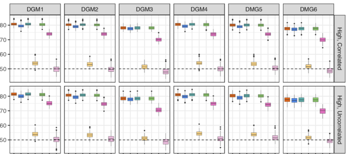
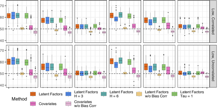
Figure S.1: Predictive Performance of Alternative Approaches in Simulations. AUROC across all pairs of species with an unrecorded interaction by method and simulation scenario. The methods considered are shown using different colors on the x-axis and they are described in Supplement E.

First, we note that the models that do not perform bias correction for taxonomic and geographical bias have extremely poor performance in all scenarios. The AUROC for the models without bias correction decreases with observational effort (not shown here). This is expected since the models without bias correction do not incorporate any information on how many times an interaction had the opportunity to be recorded or not. These results illustrate that bias correction is crucial for properly understanding species interactivity.

Second, we see that the model with $H=3$ and without using the shrinkage prior generally performs worse or as well as the same model with $H=6$, or as the model which uses the shrinkage prior. The model with $H=6$ performs comparably to the model that sets $H=10$ and uses the shrinkage prior. (We found that the model that sets $H=9$ and does not use the shrinkage prior performs similarly to the model with $H=6$, though the results are not shown here for brevity.) Therefore, we find that the shrinkage prior effectively reduces the size of the parameter space when possible, while providing the required flexibility when a higher number of latent factors is needed, without having the explicitly specify the effective number of latent factors.

Even though it is not immediately visible from the plot because the differences are small, we found that allowing for the parameters $\tau$ to vary only improved the performance of the proposed model. This reflects that the additional flexibility offered by parameter-specific $\tau$ values is useful in improving our predictions.

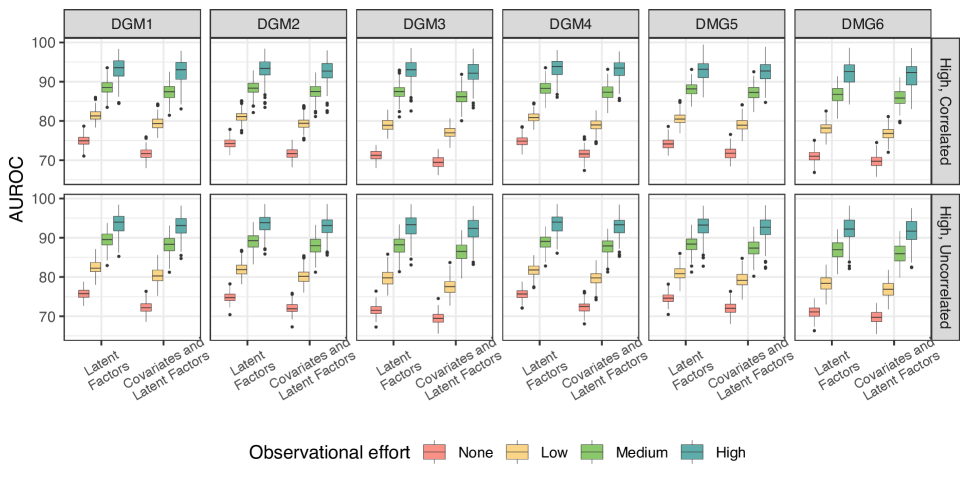
Figure S.2: Predictive Performance of Model with Covariates and Latent Factors. AUROC across four levels of pair observational effort. The model is introduced in Supplement E.

We also investigated the performance of a model that includes both covariates and latent factors in the interaction submodel. Our interest in this model stems mostly from understanding its performance when evaluating the variables’ importance for forming interactions, as it is easier to study the coefficients of the covariates in this model, compared to our approach to variable importance introduced in Section 4. Before we investigate the performance of this model for variable importance, we see that the performance of the model that incorporates both covariates and latent factors for predicting possible interactions, shown in Figure S.2, is between the performance of the covariates and latent factor models. The AUROC achieved by this model is higher than that of the covariates model, but the latent factor model introduced in Section 3 still outperforms it. We investigate the performance of this model for variable importance in Supplement F.5.

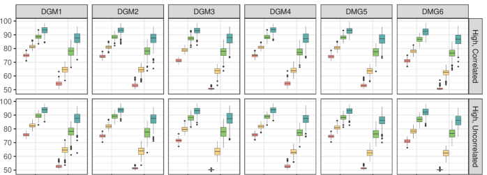
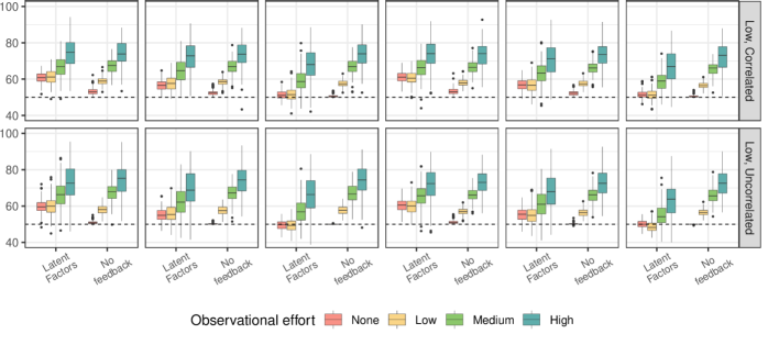
Figure S.3: Predictive Performance in Simulations. The methods considered (shown on the horizontal axis) are the proposed model (Latent Factors) and a modularized version of the same model that cuts the feedback from the interaction and detectability submodels into the latent factors (No Feedback). The columns represent the 6 DGMs in Table 1. The rows correspond to combinations of the high and low signal scenarios and the two correlation values. Results are shown by observational effort for pairs of species by color.

Lastly, we compared our model as proposed, to a modularized version of our model that bases the latent factor updates solely on the covariate model Equation 4 fit, and cuts the feedback from the interaction and detectability submodels in Equation 5 and Equation 6 into the latent factors. By comparing the results of our model to the modularized version of the same model we essentially evaluate the extent to which the full model can harvest information from the measured interactions in informing the latent factors (since the modularized model does not do so). The results from this comparison are shown in Figure S.3, across all 24 scenarios we considered and by pair-specific observational effort. In all the high-information scenarios, the full model (that allows for feedback) always performs better than the model that cuts the feedback. This illustrates that, in these scenarios, the latent factors are indeed informed by the measured interactions in a useful manner in order to predict missing interactions. In the low information setting, the version of the model that cuts the feedback can perform better than the model that allows for feedback, but only for pairs of species with a lot of observational effort. This illustrates that there can be some efficiency loss in trying to learn the latent factors using the measured interaction profiles, if those measured interactions are very sparse. However, the model that does allow for feedback performs at least as good, and often much better across all scenarios for pairs of species with no observational effort (shown in red in Figure S.3). This indicates that using the measured interaction profiles for learning the latent factors can be useful for learning about pairs of species that are rare and not well-represented in the data.

Table S.3: Number of simulated data sets with effective dimension of the latent space that is at least three. Results are shown for DGM 1, 2, 4, and 5, for the high information scenario with uncorrelated covariates. Total number of simulated data sets is 200.

		Are the same covariates important in
		interaction and detectability submodels?
are the important
covariates measured?		same	different
all		(DGM 1)	(DGM 4)
	with feedback:	11	23
	without feedback:	14	11
some		(DGM 2)	(DGM 5)
	with feedback:	8	23
	without feedback:	6	2

We also investigated the effective dimension of the latent space in DGMs 1, 2, 4, and 5 in the high information scenario with uncorrelated covariates. Here, we define the effective number to be the number of $\theta_{h}$ with posterior mean above 0.05, when $\theta_{\infty}$ is set to 0.01. In Table S.3 we report the number of simulated data sets (out of 200) where the effective dimension was at least three. When the same versus different covariates are important in the interaction and detectability submodels (comparing DGM 1 to DGM 4, and DGM 2 to DGM 5), the modularized approach that cuts the feedback uses at least three latent factors in a similar proportion of simulated data sets. In contrast, the approach that allows for feedback uses a high number of latent factors more frequently when different covariates are important in the two submodels, illustrating that by allowing for feedback the effective dimension of the latent factor space can be larger if needed in order to capture the important information.

F.4   Simulation results for out of sample species

Out-of-sample species are species with zero observational effort: species that could not have been recorded in an interaction with any other species and in any other study. For out-of-sample species, we might be interested in predicting their interactions with other out-of-sample species, or with in-sample species. Pairs for which both species are out-of-sample are referred to as “out-of-sample” pairs, and pairs of species for which one is in-sample and the other is out-of-sample are referred to as “half-in-sample”. Results for the high information scenarios for the latent factor and covariates approaches in terms of AUROC achieved are shown in Figure S.4.

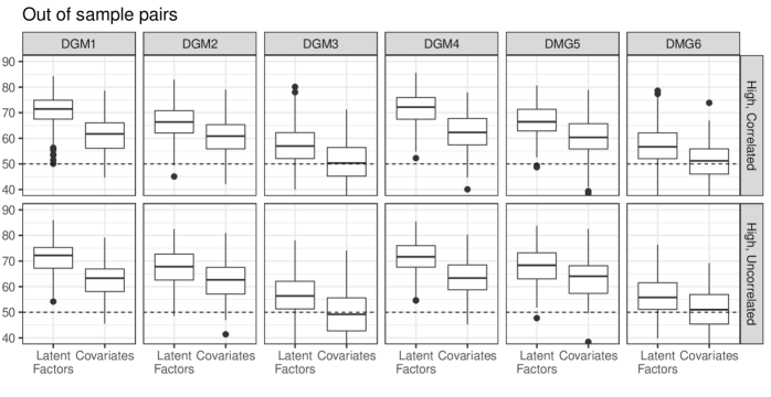
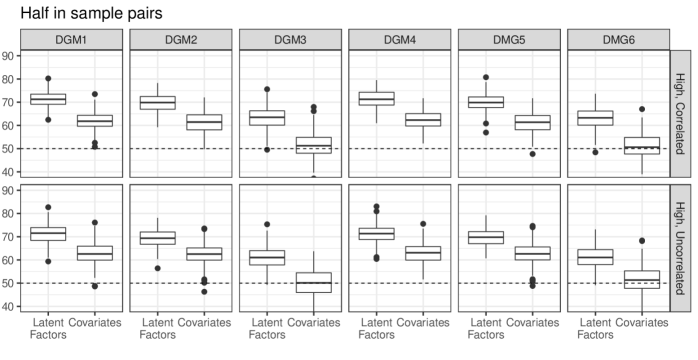
Figure S.4: Predictive Performance of Latent Factor and Covariate Approaches for Out of Sample Species. Results shown for the high information scenario, all DGMs and both correlations. The out of sample species are considered in combination with other out of sample species (rows 1 & 2) and in combination with in sample species (rows 3 & 4).

Again, the latent factor model performs better than the covariates model in all scenarios considered. We also investigate performance of the latent factor approach for out of sample species. The pairs of species without a chance of being detected in an interaction are of the following types: (a) in-sample pairs that have zero observation effort between them but non-zero observational effort with other species (illustrated in Figure 2 as observation effort ‘none’), (b) half in sample pairs, and (c) out of sample pairs. We see that the AUROC achieved by the latent factor approach is better for in-sample pairs without observational effort, then for half in sample pairs, and then for out of sample pairs. This illustrates that the latent factor approach learns about a species’ possible interactions through its interactions with other species. Conclusions from the low information scenarios are similar though less visible since the approaches have AUROC closer to 50% even for in-sample pairs of species.

F.5   Simulation results on variable importance

F.5.1   Based on the latent factor model

We performed simulations to investigate the performance of the variable importance measure of Section 4. We considered all the simulation scenarios from the main text, though we focus here on the high information scenarios for brevity.

Figures S.5 and S.6 show the results for the first and second sets of species, respectively. Specifically, each panel corresponds to a different combination of covariate and DGM and it shows the distribution across simulated data sets of the number of permutation standard deviations away from the permutation mean that the observed statistic falls. Larger values represent that the observed covariate is more informative of the probability of forming and detecting interactions between species. Dark blue color is used for covariates that are important for both forming or detecting interactions, light blue is used for covariates that are important only for forming interactions, green is used for covariates that are important only for detecting interactions, and red is used for covariates that are important for neither. The importance of each covariate is also shown in Table 1. For the first set of species, covariates 1 and 2 are continuous and the rest binary, and for the second set of species covaraites 1 through 4 are continuous and the rest are binary.

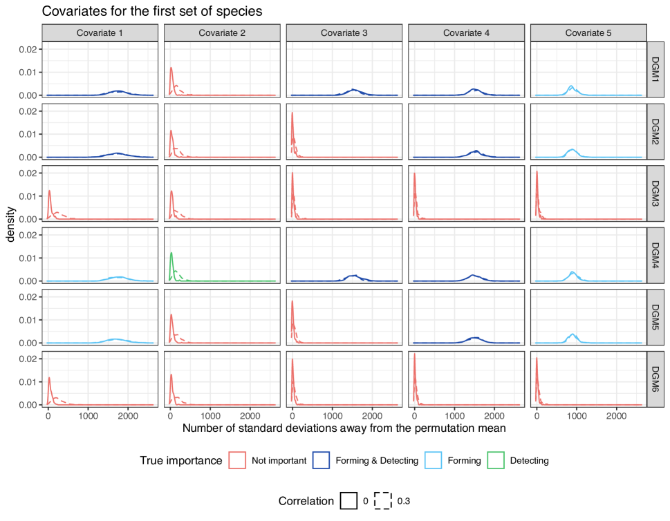
Figure S.5: Variable importance simulations for the first set of species. Number of standard deviations away from the permutation mean by covariate and data generative model. Different colors are used for variables of different importance (important or not for forming and/or detecting an interaction), in agreement with Table 1. Different line type is used for the scenarios with correlated (dashed) and uncorrelated (solid) covariates.

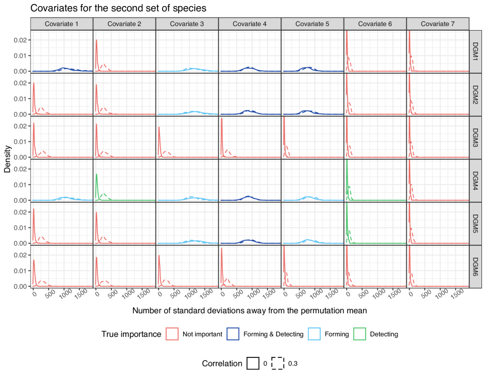
Figure S.6: Variable importance simulations for the second set of species. Number of standard deviations away from the permutation mean by covariate and data generative model. Different colors are used for variables of different importance (important or not for forming and/or detecting an interaction), in agreement with Table 1. Different line type is used for the scenarios with correlated (dashed) and uncorrelated (solid) covariates. Results for plant covariates 8, 9, 11, and 12 are similar to those of covariate 7 and are excluded.

Focusing first in the case with uncorrelated covariates, we find that the histograms for covariates that are not important for forming interactions are concentrated near 0 standard deviations, implying that the observed statistic resembles that of the permuted data sets. This means that the approach correctly identifies covariates that are not important for forming interactions, irrespective of whether these covariates are important for detection or not, and covariates that only drive detectability are not identified as important based on this variable importance metric. In contrast, the histograms for covariates that are important for forming interactions are always well-separated from zero, and correctly identified. We find that continuous variables tend to have higher variable importance scores than binary variables with the same importance (for example, compare the results for covariates 1 & 3 of DGM1 of the bird species, and covariates 4 & 5 of DGM1 for the plant species). Therefore, it might be preferable to focus on variable importance separately for continuous and binary covariates.

Unsurprisingly, when there is correlation among the covariates, the covariates that are not important are correlated with the important ones. Therefore, we see higher variable importance metrics in this case for the unimportant covariates. The variable importance metric for the important covariates remains unaltered.

F.5.2   Based on the model that includes covariates and latent factors

To study variable importance based on the model that includes both covariates and latent factors, we investigated the 95% credible intervals for the coefficients of the covariates. We show here the results for the high information scenarios with uncorrelated covariates. The high information scenarios with uncorrelated covariates can be seen as the “easiest” setting for identifying variable importance.

Table S.4: Variable importance for the model with covariates and latent factors. Percentage of 200 data sets where the 95% credible interval for the coefficient of each covariate did not include zero, and the covariate was deemed important. Values close to 1 indicate that the covariate was identified as important in most data sets. Results correspond to the high information scenario with all covariates uncorrelated.

	DGM1	DGM2	DGM3	DGM4	DGM5	DGM6
$X_{1}$	0.295	0.320	0.275	0.245	0.215	0.250
$X_{2}$	0.060	0.065	0.525	0.155	0.085	0.640
$X_{3}$	0.290	0.055	0.220	0.265	0.060	0.290
$X_{4}$	0.645	0.575	0.255	0.595	0.530	0.180
$X_{5}$	1.000	1.000	0.250	1.000	1.000	0.320
$W_{1}$	0.570	0.060	0.150	0.455	0.045	0.115
$W_{2}$	0.045	0.050	0.165	0.300	0.080	0.145
$W_{3}$	0.990	0.985	0.185	0.990	0.995	0.120
$W_{4}$	0.995	0.985	0.230	1.000	0.985	0.155
$W_{5}$	1.000	1.000	0.060	1.000	1.000	0.085
$W_{6}$	0.080	0.055	0.100	0.085	0.090	0.095
$W_{7}$	0.040	0.040	0.075	0.020	0.050	0.125
$W_{8}$	0.085	0.045	0.100	0.060	0.045	0.060
$W_{9}$	0.025	0.055	0.110	0.020	0.040	0.115
$W_{10}$	0.040	0.050	0.140	0.050	0.055	0.090
$W_{11}$	0.015	0.085	0.050	0.025	0.055	0.135
$W_{12}$	0.060	0.070	0.645	0.050	0.045	0.440

Results are shown in Table S.4. We see that many covariates that are completely unrelated with species interactivity are identified as important very often. For example, the binary covariate $W_{12}$ that is unrelated to everything, is identified as important in 88 of the 200 data sets from DGM6. If this method for variable importance performed accurately, each null covariate would be identified as important in 5% of data sets or fewer. However, we see that the proportion of data sets that identify null covariates as important is almost always higher than 5%. We believe that this is due to collinearity between the phylogenetically-correlated latent factors and phylogenetically-correlated covariates, which leads to issues similar to those of spatial confounding in the spatial literature.

F.6   Computational time of the proposed approach

We investigated the computational time for 1,000 posterior samples of our approach when varying the number of bird species, number of plant species, and the number of studies. We considered number of birds equal to 50, 100, 150, and 200, number of plants equal to 50, 200, 350, and 500, and number of studies equal to 10, 40, and 80. For each combination of number of species and studies, we ran a mini-simulation with 10 data sets and 1,000 posterior samples each. The median computational time across the 10 data sets is shown in Table S.5. The computational time appears to grow linearly in the total number of pairs ($n_{B}\times n_{P}$), whereas the number of measured networks ($S$) does not appear to affect computational time.

Table S.5: Computational time of 1,000 MCMC iterations when varying the number of species and number of studies. $S$ represents the number of studies, $n_{B}$ the number of species of the first set (birds) and $n_{P}$ the number of species of the second set (plants).

		50	200	350	500
$S=10$
	50	2.02	6.58	16.39	21.42
	100	3.44	13.80	24.80	35.71
	150	4.66	17.46	24.59	36.26
	200	9.98	25.77	50.19	75.55
$S=40$
	50	2.06	6.62	13.89	31.00
	100	3.36	14.08	24.48	37.97
	150	4.92	17.91	27.38	37.37
	200	9.56	32.93	51.91	84.85
$S=80$
	50	1.85	6.84	13.67	21.18
	100	3.50	16.20	27.08	49.02
	150	5.26	17.33	22.85	58.47
	200	7.19	30.05	54.23	72.50

Appendix G Out-of-sample species

Our main focus is in predicting whether a species $i^{*}$ with covariates $\bm{X}_{i^{*}}$ would interact with a species $j^{*}$ with covariates $\bm{W}_{j^{*}}$ if given the opportunity, where the covariates might be available with missingness. If both species are included in the original $n_{B}\times n_{P}$ data, predictions are automatic based on the posterior samples of $\bm{L}$. However, species might be completely unobserved and have no recorded interactions, and we might be interested in understanding whether these out-of-sample species interact with all other species.

G.1   The posterior distribution for the presence of interaction for species with unrecorded interactions

Inference on the probability of interaction between species $i^{*}$ and $j^{*}$ when neither of them has any recorded interactions could proceed by extending the observed interaction matrix of $n_{B}$ and $n_{P}$ species to an $(n_{B}+1)\times(n_{P}+1)$ interaction matrix with $n_{i^{*}j}=0$ and $n_{ij^{*}}=0$ for all $i,j$ species in the original data set, and re-fitting the MCMC.

By investigating the posterior probability that these out-of-sample species interact, we better understand how the model borrows information across species. Let $\bm{\theta}^{*}$ denote all model parameters excluding parameters corresponding to the species $i^{*}$ and $j^{*}$, $\widetilde{\bm{D}}$ denote the observed data for all in-sample species, and $\bm{X}_{i^{*}}$ and $\bm{W}_{j^{*}}$ denote covariates for $i^{*}$ and $j^{*}$, respectively, where the covariate vectors can include missing values. Let $\bm{U}_{i^{*}},\bm{V}_{j^{*}}$ denote the latent factors corresponding to $i^{*},j^{*}$ respectively. Then, we wish to predict $L_{i^{*}j^{*}}$ based on what we have learnt from the observed data and from the out-of-sample species covariates. That would amount to learning $P(L_{i^{*}j^{*}}=1\mid\widetilde{\bm{D}},\bm{X}_{i^{*}},\bm{W}_{j^{*}}).$, which we rewrite as

$$P( L_{i^{*}j^{*}}=1\mid\widetilde{\bm{D}},\bm{X}_{i^{*}},\bm{W}_{j^{*}})=$$ (S.5)

$$=\int P(L_{i^{*}j^{*}}=1\mid\bm{\theta}^{*},\bm{U}_{i^{*}},\bm{V}_{j^{*}}\widetilde{\bm{D}},\bm{X}_{i^{*}},\bm{W}_{j^{*}})\ p(\bm{\theta}^{*},\bm{U}_{i^{*}},\bm{V}_{j^{*}}\mid\widetilde{\bm{D}},\bm{X}_{i^{*}},\bm{W}_{j^{*}})\ \mathrm{d}(\bm{\theta}^{*},\bm{U}_{i^{*}},\bm{V}_{j^{*}})$$

$$\propto\int P(L_{i^{*}j^{*}}=1\mid\bm{\theta}^{*},\bm{U}_{i^{*}},\bm{V}_{j^{*}})\ p(\bm{X}_{i^{*}},\bm{W}_{j^{*}}\mid\bm{\theta}^{*},\bm{U}_{i^{*}},\bm{V}_{j^{*}}\widetilde{\bm{D}})\ p(\bm{\theta}^{*},\bm{U}_{i^{*}},\bm{V}_{j^{*}}\mid\widetilde{\bm{D}})\ \mathrm{d}(\bm{\theta}^{*},\bm{U}_{i^{*}},\bm{V}_{j^{*}})$$

$$\propto\int\overbrace{P(L_{i^{*}j^{*}}=1\mid\bm{\theta}^{*},\bm{U}_{i^{*}},\bm{V}_{j^{*}})}^{(A)}\ \overbrace{p(\bm{X}_{i^{*}}\mid\bm{\theta}^{*},\bm{U}_{i^{*}})\ p(\bm{W}_{j^{*}}\mid\bm{\theta}^{*},\bm{V}_{j^{*}})}^{(B)}$$

$$\hskip 142.26378pt\underbrace{p(\bm{U}_{i^{*}},\bm{V}_{j^{*}}\mid\bm{\theta}^{*})}_{(C)}\ \underbrace{p(\bm{\theta}^{*}\mid\widetilde{\bm{D}})}_{(D)}\ \mathrm{d}(\bm{\theta}^{*},\bm{U}_{i^{*}},\bm{V}_{j^{*}}).$$

In (A) we see that having access to the species’ latent factors would allow us to straightforwardly learn their probability of interaction. Therefore, ideally one could draw the species’ latent factors from their posterior distribution, and draw their interaction indicator from the corresponding conditional distribution in (A). In that sense, estimation of interaction probabilities for out-of-sample units resembles outcome prediction in mixed models for new units for which the random effect is drawn from the common random effect distribution. The main difference between these parallel settings arise from parts (B) and (C) in Equation S.5. Factor (B) tells us that the latent factors for the new species are driven by the latent factors for the in-sample species since their correlation matrix is non-diagonal, and factor (C) tells us that the latent factors for the out-of-sample species needs to also agree with the species’ observed covariates. Therefore, learning the interaction probability of out-of-sample species is based largely on the interaction profiles of phylogenetically related species and the species’ covariate profile.

G.2   Computationally efficient algorithm for out-of-sample prediction of species interactions

Here, we introduce an alternative approach for acquiring out-of-sample predictions of species interactions which avoids re-fitting the MCMC for every new species. We propose a computationally efficient algorithm for making predictions for out-of-sample species, which combines the MCMC fit to the original data and importance sampling weighting. Expression Equation S.5 is the basis of our algorithm. We first describe the algorithm here, and then we provide the explicit steps for its implementation afterwards. We use draws from the posterior distribution of model parameters based on the original data (D) to draw latent factors for the species $i^{*},j^{*}$ (C) where the correlation matrices $\bm{C}_{U},\bm{C}_{V}$ are updated to include the new species. Based on the latent factors and the model parameters of each posterior sample, we draw values for the indicator of whether the species interact (A). Since these draws do not account for the covariates, we up(down)-weigh the draws which use parameters and latent factors that have higher (lower) values of (B).

To describe the algorithm in full detail, let $\bm{C}_{U}^{\ast}$, $\bm{C}_{V}^{\ast}$ be the extended correlation matrices with units $i^{*}$ and $j^{*}$ included. Then $\bm{C}_{U}^{\ast}$, $\bm{C}_{V}^{\ast}$ are correlation matrices of dimension $n_{B}+1$ and $n_{P}+1$, and the upper left $n_{B}\times n_{B}$ and $n_{P}\times n_{P}$ submatrices are $\bm{C}_{U}$, $\bm{C}_{V}$, respectively. In what follows the superscript $(r)$ represents the $r^{th}$ posterior sample from the MCMC out of a total of $R$ samples. The algorithm is as follows:

1. First, we acquire samples for the species’ latent factors based on samples from the posterior distribution of model parameters $\bm{\theta}^{*}{}^{(r)}$, $r=1,2,\dots,R$. We do so as follows:

   • For $r=1,2,\dots,R$, we generate latent factors $U_{i^{*}h}$ for species $i^{\ast}$ from $N(\mu,\sigma^{2})$ where

     $$\sigma^{2}=\big{[}S^{(r)}\big{]}_{(n_{B}+1),(n_{B}+1)}-\big{[}\bm{S}^{(r)}\big{]}_{(n_{B}+1),(1:n_{B})}\left[\big{[}\bm{S}^{(r)}\big{]}_{(1:n_{B}),(1:n_{B})}\right]^{-1}\left[\big{[}\bm{S}^{(r)}\big{]}_{(n_{B}+1),(1:n_{B})}\right]^{T}$$

     and

     $$\mu=\big{[}\bm{S}^{(r)}\big{]}_{(n_{B}+1),(1:n_{B})}\left[\big{[}\bm{S}^{(r)}\big{]}_{(1:n_{B}),(1:n_{B})}\right]^{-1}\bm{U}_{1:n_{B},h}^{(r)},$$

     where $\bm{S}^{(r)}=\rho_{U}^{(r)}\bm{C}_{U}^{\ast}+(1-\rho_{U}^{(r)})\bm{I}_{n_{B}+1}$, $[\bm{S}^{(r)}]_{\mathcal{A},\mathcal{B}}$ represents the submatrix of $\bm{S}^{(r)}$ with row indices in $\mathcal{A}$ and column indices in $\mathcal{B}$, and $\bm{U}_{1:n_{B},h}^{(r)}=(U_{1h}^{(r)},U_{2h}^{(r)},\dots,U_{n_{B}h}^{(r)})$.

   • Generate latent factors for species $j^{*}$ similarly as for species $i^{*}$, but substituting $\bm{C}_{U}$ for $\bm{C}_{V}$, $\rho_{U}$ for $\rho_{V}$, $\bm{U}$ for $\bm{V}$, and $n_{B}$ for $n_{P}$.

   Performing these steps leads to latent factors $\bm{U}_{i^{*}}^{(r)}=(U_{i^{*}1},U_{i^{*}2},\dots,U_{i^{*}H})^{T}$ for species $i^{*}$ and $\bm{V}_{j^{*}}=(V_{j^{*}1},V_{j^{*}2},\dots,V_{j^{*}H})^{T}$ for species $j^{*}$, for all $r$. We use these latent factors to make an original set of predictions. For each $r$, we generate $\widetilde{L}_{i^{*}j^{*}}^{(r)}$ from a Bernoulli distribution with probability of success equal to $\mathrm{expit}\left(\lambda_{0}^{(r)}+\sum_{h}\lambda_{h}^{(r)}U_{i^{*}h}^{(r)}V_{j^{*}h}^{(r)}\right)$.

2. However, the generated latent factors have been sampled taking only the correlation structure of the latent factors across species into consideration, and as a result the latent factors and the predictions do not use the information on the new species’ covariates. To account for the covariates we perform importance weighting:

   • For species $i^{*}$ with generated latent factors $\bm{U}_{i^{\ast}}^{(r)}$ and covariates $\bm{X}_{i^{*}}$ calculate the importance sampling weight $w_{i^{*}}^{(r)}=w_{i^{*}1}^{(r)}w_{i^{*}2}^{(r)}\dots,w_{i^{*}p_{B}}^{(r)}$, where $w_{i^{*}m}^{(r)}$ is 1 if $X_{i^{*}m}$ is missing,

     $$w_{i^{*}m}^{(r)}=\phi\left(X_{i^{*}m};l_{i^{*}m}^{(r)},(\sigma^{2}_{m})^{(r)}\right)$$

     if the $m^{th}$ covariate is continuous, and

     $$w_{i^{*}m}^{(r)}=u(X_{i^{*}m};\mathrm{expit}(l_{i^{*}m}^{(r)}))$$

     if the $m^{th}$ covariate is binary, where $l_{i^{*}m}^{(r)}=\beta_{m0}^{(r)}+(\bm{U}_{i^{\ast}}^{(r)})^{T}\bm{\beta}_{m}^{(r)}$, $\phi(\cdot;\mu,\sigma^{2})$ is the normal density with mean $\mu$ and variance $\sigma^{2}$, and $u(\cdot;p)$ is the mass function for the Bernoulli($p$) random variable.

   • Similarly to the above, we acquire $w_{j^{*}}$ for species $j^{*}$.

   • The importance sampling weight for the pair $(i^{*},j^{*})$ is then defined as $w_{i^{*}j^{*}}^{(r)}=w_{i^{*}}^{(r)}w_{j^{*}}^{(r)}$ for $r=1,2,\dots,R$.

3. We combine these importance sampling weights with the original predicted interaction values $\widetilde{L}_{i^{*}j^{*}}^{(r)}$. Intuitively, $w_{i^{*}j^{*}}^{(r)}$ describes how in-line the generated latent factors $\bm{U}_{i^{*}}^{(r)}$ and $\bm{V}_{j^{*}}^{(r)}$ are with the species’ covariate profiles, and, in a sense, how “trustworthy” the $r^{th}$ prediction is. For this reason, we set the posterior probability for an $(i^{*},j^{*})$ interaction equal to

   $$\left(\sum_{r=1}^{R}w_{i^{*}j^{*}}^{(r)}\widetilde{L}_{i^{*}j^{*}}^{(r)}\right)\Big{/}\left(\sum_{r=1}^{R}w_{i^{*}j^{*}}^{(r)}\right).$$

For making interaction predictions for pairs of species of which one is in the original data set and the other one is not, the algorithm is very similar. For the in-sample species, samples from the posterior distribution for its latent factors are already acquired through the MCMC. Therefore, the procedure above only has to be performed for the species that are out-of-sample, and the importance sampling weights only represent one of the species. For example, if $i^{*}$ is included in the original data and $j^{*}$ is out-of-sample, then we use the algorithm described above to acquire $\bm{V}_{j^{*}}^{(r)}$, $w_{j^{*}}{(r)}$, and $\widetilde{L}_{i^{*}j^{*}}^{(r)}$ and set $w_{i^{*}j^{*}}^{(r)}=w_{j^{*}}^{(r)}$.

G.3   How out-of-sample species might affect predictions for in-sample species

Availability of covariate information on the new species requires that we also update our predictions for in-sample species. Therefore, when covariate data on $i^{*},j^{*}$ become available, the posterior for $\bm{\theta}^{*}$ should be

$$p(\bm{\theta}^{*}\mid\widetilde{\bm{D}},\bm{X}_{i^{*}},\bm{W}_{j^{*}}) \propto p(\widetilde{\bm{D}}\mid\bm{\theta}^{*},\bm{X}_{i^{*}},\bm{W}_{j^{*}})\ p(\bm{X}_{i^{*}},\bm{W}_{j^{*}}\mid\bm{\theta}^{*})\ p(\bm{\theta}^{*})$$ (S.6)

$$=p(\widetilde{\bm{D}}\mid\bm{\theta}^{*})\ p(\bm{X}_{i^{*}},\bm{W}_{j^{*}}\mid\bm{\theta}^{*})\ p(\bm{\theta}^{*})$$

$$=p(\bm{\theta}^{*}\mid\widetilde{\bm{D}})\ \frac{p(\bm{\theta}^{*}\mid\bm{X}_{i^{*}},\bm{W}_{j^{*}})}{p(\bm{\theta}^{*})}$$

$$=p(\bm{\theta}^{*}\mid\widetilde{\bm{D}})\ \int\frac{p(\bm{\theta}^{*}\mid\bm{\theta}^{*}_{i^{*},j^{*}})}{p(\bm{\theta}^{*})}p(\bm{\theta}^{*}_{i^{*},j^{*}}\mid\bm{X}_{i^{*}},\bm{W}_{j^{*}})\ \mathrm{d}\bm{\theta}^{*}_{i^{*},j^{*}},$$

where we use $\bm{\theta}^{*}_{i^{*},j^{*}}$ to denote all model parameters for species $i^{*},j^{*}$ (includes latent factors and detection probability). Intuitively, the covariates $\bm{X}_{i^{*}},\bm{W}_{j^{*}}$ drive estimation of the latent factors for $i^{*},j^{*}$ (last term in Equation S.6), and correlation of the latent factors across species would imply that the latent factors for $i^{*},j^{*}$ affect the latent factors for in-sample species and $p(\bm{\theta}^{*}\mid\bm{\theta}^{*}_{i^{*},j^{*}})\ /\ p(\bm{\theta}^{*})\neq 1$. Therefore, the integral in Equation S.6 will not be equal to 1, and the posterior distribution that incorporates the new covariate values, $p(\bm{\theta}^{*}\mid\widetilde{\bm{D}},\bm{X}_{i^{*}},\bm{W}_{j^{*}})$, will not be the same as the original posterior distribution, $p(\bm{\theta}^{*}\mid\widetilde{\bm{D}})$.

Appendix H Additional study results

H.1   Comparison of results from the two models

Figure S.7 shows the posterior probability that an interaction between two species is possible based on our approach and the alternative approach that uses covariates directly. Vertical and horizontal blue lines separate different taxonomic families. A list of all the species included in our analysis in the same ordering as shown in the results is included in Supplement J. The same conclusions discussed in Section 6 also hold when showing the full set of species.

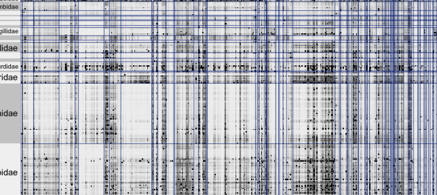
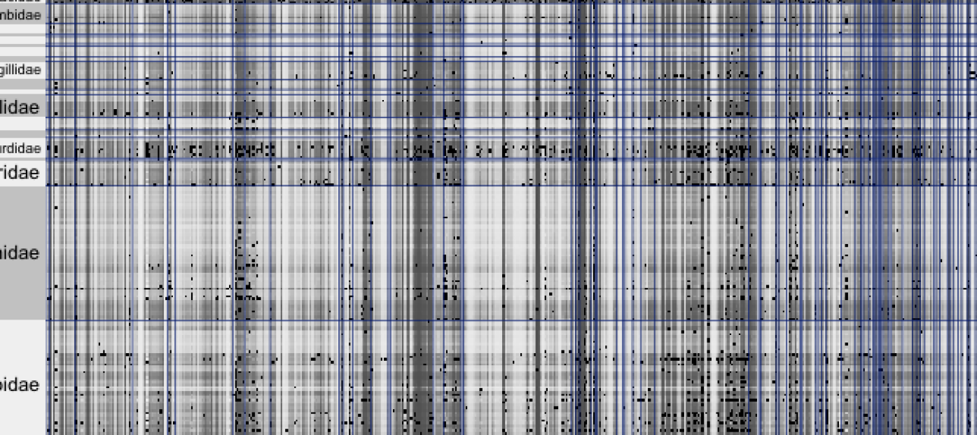
Figure S.7: Posterior Probability of Possible Interactions for all bird (y-axis) and plant (x-axis) species. Species are organized in taxonomic families separated by blue lines. Black color shows the recorded interactions.

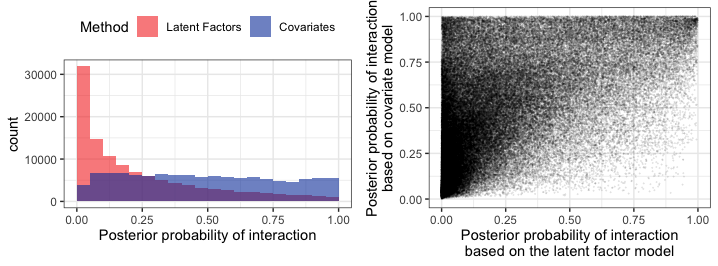
Figure S.8: Comparison of Model Predictions. Values close to 1 indicate that an interaction between the two species is likely to be possible. Observed interactions are excluded from the plot. (Left) Histograms of posterior interaction probabilities for all pairs of species without a recorded interaction based on the two models. (Right) The predictions from the two models are plotted against each other.

We further compare results from the two models in Figure S.8. On the left, we see that the model that employs covariates directly returns posterior probabilities of interaction that are above 0.5 for approximately half of the pairs. In contrast, our model predicts that a non-negligible, but more realistic, proportion of pairs are interactive. Furthermore, our model identifies a large number of pairs which are likely impossible to interact (41% of pairs have posterior probability of interaction that is below 0.1) in contrast to the covariate model (9% of pairs).

We study the model predictions against each other in the right side of Figure S.8. We focus on pairs that are likely/not likely to interact, defined as pairs with posterior probability of interaction ranging between 0–0.1 and 0.9–1, respectively. We find that the two models sometimes return opposite conclusions, though, when that happens, the covariate model has posterior probabilities close to 1 and the latent factor model close to 0. This pattern is more general, in that the latent factor model almost always returns posterior probabilities of interaction that are lower than those based on the covariate model. The disagreement in models’ prediction, in combination with the unrealistically high number of pairs predicted to interact based on the covariates model and the cross-validation results lead us to believe that the predictions of truly interactive pairs based on the covariates model are not trustworthy. Therefore, we turn our attention to investigating the models’ relative performance in identifying pairs that are unlikely to interact. 89% of the pairs of species which the covariates model identifies as unlikely to interact are also identified as unlikely to interact based on the latent factor model. Moreover, model predictions for these pairs are substantially more precise based on the latent factor model with a median posterior standard deviation equal to 0.13, compared to 0.24 for the covariate model. Reversely, pairs of species that are unlikely to interact based on our model often also have low probability of interaction according to the covariates model. However, for these pairs, the posterior probabilities of interaction based on the covariate model range more widely over 0–0.5, with 20% of them being below 0.1 and 76% below 0.5. Therefore, even though the models seem to partially agree on which pairs of species do not interact, the latent factor model is more confident in these predictions.

The latent factor model also has an overall lower posterior uncertainty in estimated probabilities of interaction than the covariate model, average posterior standard deviation equal to 0.31 and 0.39, respectively.

Figure S.9 shows visually the cross-validation results discussed in Section 6.1. We see that, for both approaches, the ratio of posterior probability of interaction for the held-out pairs compared to all pairs is above 1, indicating that both of them assign higher posterior probability to the pairs that are known to interact. However, the ratio is much higher for the latent factor approach illustrating that it separates pairs that interact from those that do not more effectively than the approach that uses covariates.

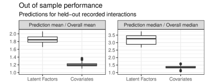
Figure S.9: Cross Validation Results. For each data set, we calculate the mean and median of the posterior interaction probability in the held-out pairs, and in the overall population. The plot shows boxplots for the ratio of held-out to overall mean (left) and median (right) by model. Higher values indicate that the true interactions were identified more clearly.

H.2   Results based on alternative specification of intra-species correlations

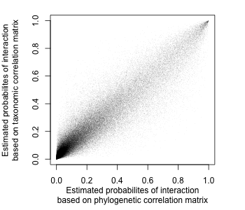
Figure S.10: Estimated probabilities of pair interaction using our model with a phylogentic correlation matrix (x-axis) and a taxonomic correlation matrix (y-axis).

To evaluate the robustness of our results to alternative specifications of intra-species dependencies, we also fit our model with taxonomically-structured correlation matrices. For bird species $i,i^{\prime}$, we specify $[C_{U}]_{ii^{\prime}}=0$ if the species are unrelated, $[C_{U}]_{ii^{\prime}}=1$ if $i=i^{\prime}$, and $[C_{U}]_{ii^{\prime}}$ equal to 0.75, 0.5, and 0.25 if the species belong to the same genera (very similar), family (similar), or order (somewhat similar), respectively. We use a similar specification for $\bm{C}_{V}$, where plant species are organized in genera and genera in families. In Figure S.10 we show the estimated probabilities of interaction based when using the taxonomically-based and the the phylogenetically-based correlation matrices. The estimated probabilities are centered and close to the 45 degree line. When regressing the estimated probabilities using the phylogenetic matrix on the estimated probabilities using the taxonomic matrix, the intercept is estimated to be -0.003 (very close to 0), and the slope is estimated to be 0.995 (very close to 1), also illustrating that the models return very similar estimated probabilities of interaction. Therefore, the method is rather robust to the codification of intra-species dependencies. We investigate the out-of-sample predictive accuracy when we use taxonomically-structured correlation matrices in Supplement H.3 and Table S.6.

H.3   The information content of species traits and phylogenetic information for predicting missing interactions

Our variable importance procedure orders the traits in terms of their importance for predicting interactions. In order to study the information content of species’ traits and phylogenetic information for predicting missing interactions, we alter the cross-validation study discussed in Section 6.1. In terms of traits, we focus on the top continuous traits for birds and plants: bird body mass and plant fruit diameter.

Our procedure is as follows: We hold out 100 measured interactions by setting the corresponding $A_{ijs}=0$ for all $s$. We fit our approach when using all the covariates, when using all the covariates excluding bird body mass, when using all the covariates excluding plant fruit diameter, and when using our approach while setting the correlation parameters in the latent factor correlation matrix $\rho_{U},\rho_{V}$ to zero. For each model fit, we calculate the average and median posterior probability of interaction for the 100 held-out pairs, and the average and median posterior probability of interaction for all pairs with an unrecorded interaction. The latter set necessarily includes pairs that are not able to interact. Therefore, if the model can separate truly interacting pairs from non-interacting pairs the ratio of these two quantities would be large. We repeat this procedure 30 times, each time holding out a different set of 100 interacting pairs. We calculate the average of the ratio of average posterior probabilities and median posterior probabilities.

The results are shown in Table S.6. We find that when considering the average posterior probability of interaction, all three sets of covariates (a, b, c) perform similarly. However, when studying the ratio of median posterior probabilities for the held-out pairs and for all pairs, the approach’s performance when we exclude fruit diameter (c) is relatively lower than the approach’s performance when we use all the covariates (a). In contrast, the approach’s performance is similar when we use all the covariates and when we exclude body mass. This is true despite the fact that there are substantially more covariates available for plants (12) compared to birds (5), and despite the fact that fruit length is also available in our data (correlation of fruit diameter and length is 0.72). These results suggest that fruit diameter is an important covariate to measure when predicting missing species’ interactions. The importance of measuring fruit diameter might be even stronger if the highly-correlated covariate representing fruit length was excluded.

Table S.6: Cross validation results to assess fit improvement attributed to different traits and phylogenetic information. Larger values imply that the approach can better differentiate truly interacting pairs from the set of pairs without a recorded interaction. The approaches considered are the following (as shown in the table): (a) the proposed approach using all covariates and phylogenetic correlation matrix for the latent factors, (b) the proposed approach excluding body mass but using the phylogenetic correlation matrix, (c) same as above but excluding fruit diameter, (d) the proposed approach will all covariates but without a phylogenetic correlation matrix ($\rho_{U},\rho_{V}=0$), (e) the proposed approach will all covariates but replacing the phylogenetic correlation matrix with a taxonomic correlation matrix, and (f) the model that is based directly on covariates.

		Ratio of averages	Ratio of medians
(a)	Latent factor model	1.85	3.19
	(all covariates, phylogeny)
(b)	Latent factor model	1.86	3.17
	excluding body mass
(c)	Latent factor model	1.84	3.06
	excluding fruit diameter
(d)	Latent factor model	1.45	1.66
	excluding phylogenetic information
(e)	Latent factor model	1.79	2.71
	using taxonomic information
(f)	Covariate model	1.21	1.36

Similarly, we notice that the approach’s ability in predicting missing interactions is much worse when no aspect of phylogenetic information is used. In Table S.6 we compare the complete model (a), with the model that does not use phylogenetic information by setting $\rho_{U},\rho_{V}=0$ (d), and the model that uses taxonomic information instead of phylogenetic information (e). We see that using taxonomic information performs worse than using phylogenetic information, and that using no phylogenetic or taxonomic information at all shows significant loss in predictive accuracy. Therefore, incorporating species’ phylogenetic relationships is important for predicting missing interactions. We note here that even when phylogenetic information is completely excluded (d), the latent factor model performs better than the model that uses covariates directly (f).

Appendix I MCMC diagnostics

We evaluated convergence of MCMC scheme by studying traceplots of identifiable parameters across chains. Since latent factors and their corresponding coefficients are not identifiable, we focused our attention to: linear predictors and residual variances for the trait models, probabilities of detection and residual variances for both sets of species, and the correlation parameters $\rho_{U},\rho_{V}$ in the latent factors’ covariance structure across species in the same set. The traceplots for a subset of parameters are shown in Figures S.12, S.12, S.14, and S.14. Overall convergence seems to be good. We observe some autocorrelation in the posterior samples for the latent factor correlation parameters $\rho$, but mixing seems to be good, and the values over which the MCMC concentrates are similar and very close to 1. We also investigated running means for the interactions indicators. If the posterior distribution is unimodal and the MCMC has converged sufficiently well, the running means converge to the same point. Running means for nine pairs of species without a recorded interaction are shown in Figure S.15.

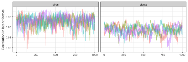
Figure S.11: Detectability scores for four randomly chosen birds. Traceplots for the linear predictor (Row 1) and posterior samples (Row 2). Colors correspond to different MCMC chains.

Figure S.12: Correlation of latent factors. Traceplots showing MCMC samples from the posterior distributions of $\rho_{U}$ (left) and $\rho_{V}$ (right). Colors correspond to different MCMC chains.

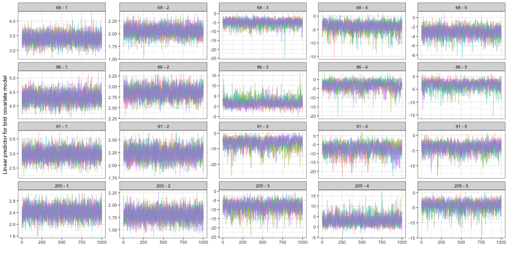
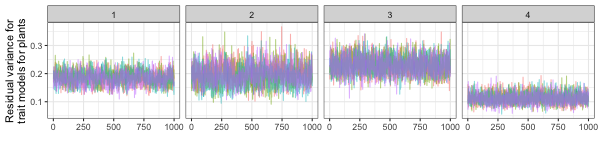
Figure S.13: Linear predictor of trait models for bird species. Traceplots for the linear predictor of all traits for four randomly chosen species of birds. The rows correspond to different bird species and the columns correspond to observed traits. The first two traits are continuous and the last three traits are binary.

Figure S.14: Residual variances of continuous traits for plant species.

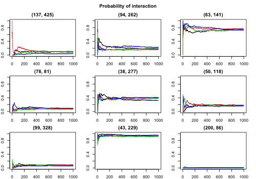
Figure S.15: Probability of species interaction. Running means of the indicator $L_{ij}$ representing whether species $i,j$ interact. Running means are shown for nine pairs of species without a recorded interaction.

Appendix J List of all species included in our analysis

Tables LABEL:supp_tab:bird_species and LABEL:supp_tab:plant_species show the bird and plant species, respectively, that are included in our analysis along with their taxonomic information. The column “Included” denotes whether the species are shown in the results of the main text or not. The species are listed in the same order shown in the results of Section 6 and Supplement H.

Table S.7: Bird species included in our data and their taxonomic information.

Species	Order	Family	Genus	Included
Pyroderus scutatus	Passeriformes	Cotingidae	Pyroderus	X
Pachyramphus validus	Passeriformes	Cotingidae	Pachyramphus	X
Pachyramphus castaneus	Passeriformes	Cotingidae	Pachyramphus	X
Pachyramphus viridis	Passeriformes	Cotingidae	Pachyramphus	X
Pachyramphus polychopterus	Passeriformes	Cotingidae	Pachyramphus	X
Lipaugus lanioides	Passeriformes	Cotingidae	Lipaugus	X
Lipaugus vociferans	Passeriformes	Cotingidae	Lipaugus	X
Tityra cayana	Passeriformes	Cotingidae	Tityra	X
Tityra inquisitor	Passeriformes	Cotingidae	Tityra	X
Oxyruncus cristatus	Passeriformes	Cotingidae	Oxyruncus	X
Carpornis cucullata	Passeriformes	Cotingidae	Carpornis	X
Carpornis melanocephala	Passeriformes	Cotingidae	Carpornis	X
Schiffornis virescens	Passeriformes	Cotingidae	Schiffornis	X
Procnias nudicollis	Passeriformes	Cotingidae	Procnias	X
Tijuca atra	Passeriformes	Cotingidae	Tijuca	X
Phibalura flavirostris	Passeriformes	Cotingidae	Phibalura	X
Laniisoma elegans	Passeriformes	Cotingidae	Laniisoma	X
Cacicus haemorrhous	Passeriformes	Icteridae	Cacicus
Cacicus chrysopterus	Passeriformes	Icteridae	Cacicus
Chrysomus ruficapillus	Passeriformes	Icteridae	Chrysomus
Molothrus bonariensis	Passeriformes	Icteridae	Molothrus
Icterus cayanensis	Passeriformes	Icteridae	Icterus
Pseudoleistes guirahuro	Passeriformes	Icteridae	Pseudoleistes
Psarocolius decumanus	Passeriformes	Icteridae	Psarocolius
Gnorimopsar chopi	Passeriformes	Icteridae	Gnorimopsar
Sicalis flaveola	Passeriformes	Thraupidae	Sicalis	X
Thraupis palmarum	Passeriformes	Thraupidae	Thraupis	X
Thraupis episcopus	Passeriformes	Thraupidae	Thraupis	X
Thraupis sayaca	Passeriformes	Thraupidae	Thraupis	X
Thraupis cyanoptera	Passeriformes	Thraupidae	Thraupis	X
Thraupis ornata	Passeriformes	Thraupidae	Thraupis	X
Thraupis bonariensis	Passeriformes	Thraupidae	Thraupis	X
Tachyphonus coronatus	Passeriformes	Thraupidae	Tachyphonus	X
Tachyphonus cristatus	Passeriformes	Thraupidae	Tachyphonus	X
Tachyphonus rufus	Passeriformes	Thraupidae	Tachyphonus	X
Tangara cayana	Passeriformes	Thraupidae	Tangara	X
Tangara seledon	Passeriformes	Thraupidae	Tangara	X
Tangara mexicana	Passeriformes	Thraupidae	Tangara	X
Tangara desmaresti	Passeriformes	Thraupidae	Tangara	X
Tangara cyanocephala	Passeriformes	Thraupidae	Tangara	X
Tangara cyanoptera	Passeriformes	Thraupidae	Tangara	X
Tangara preciosa	Passeriformes	Thraupidae	Tangara	X
Tangara cyanoventris	Passeriformes	Thraupidae	Tangara	X
Tangara peruviana	Passeriformes	Thraupidae	Tangara	X
Dacnis cayana	Passeriformes	Thraupidae	Dacnis	X
Dacnis nigripes	Passeriformes	Thraupidae	Dacnis	X
Ramphocelus carbo	Passeriformes	Thraupidae	Ramphocelus	X
Ramphocelus bresilius	Passeriformes	Thraupidae	Ramphocelus	X
Thlypopsis sordida	Passeriformes	Thraupidae	Thlypopsis	X
Conirostrum speciosum	Passeriformes	Thraupidae	Conirostrum	X
Hemithraupis guira	Passeriformes	Thraupidae	Hemithraupis	X
Hemithraupis ruficapilla	Passeriformes	Thraupidae	Hemithraupis	X
Hemithraupis flavicollis	Passeriformes	Thraupidae	Hemithraupis	X
Tersina viridis	Passeriformes	Thraupidae	Tersina	X
Chlorophanes spiza	Passeriformes	Thraupidae	Chlorophanes	X
Pipraeidea melanonota	Passeriformes	Thraupidae	Pipraeidea	X
Schistochlamys ruficapillus	Passeriformes	Thraupidae	Schistochlamys	X
Schistochlamys melanopis	Passeriformes	Thraupidae	Schistochlamys	X
Cissopis leverianus	Passeriformes	Thraupidae	Cissopis	X
Orthogonys chloricterus	Passeriformes	Thraupidae	Orthogonys	X
Trichothraupis melanops	Passeriformes	Thraupidae	Trichothraupis	X
Cyanerpes cyaneus	Passeriformes	Thraupidae	Cyanerpes	X
Stephanophorus diadematus	Passeriformes	Thraupidae	Stephanophorus	X
Nemosia pileata	Passeriformes	Thraupidae	Nemosia	X
Coryphospingus cucullatus	Passeriformes	Thraupidae	Coryphospingus	X
Coryphospingus pileatus	Passeriformes	Thraupidae	Coryphospingus	X
Volatinia jacarina	Passeriformes	Thraupidae	Volatinia	X
Sporophila caerulescens	Passeriformes	Thraupidae	Sporophila	X
Sporophila nigricollis	Passeriformes	Thraupidae	Sporophila	X
Sporophila leucoptera	Passeriformes	Thraupidae	Sporophila	X
Haplospiza unicolor	Passeriformes	Thraupidae	Haplospiza	X
Orchesticus abeillei	Passeriformes	Thraupidae	Orchesticus	X
Poospiza thoracica	Passeriformes	Thraupidae	Poospiza	X
Poospiza lateralis	Passeriformes	Thraupidae	Poospiza	X
Eucometis penicillata	Passeriformes	Thraupidae	Eucometis	X
Pyrrhocoma ruficeps	Passeriformes	Thraupidae	Pyrrhocoma	X
Elaenia flavogaster	Passeriformes	Tyrannidae	Elaenia	X
Elaenia spectabilis	Passeriformes	Tyrannidae	Elaenia	X
Elaenia chiriquensis	Passeriformes	Tyrannidae	Elaenia	X
Elaenia mesoleuca	Passeriformes	Tyrannidae	Elaenia	X
Elaenia cristata	Passeriformes	Tyrannidae	Elaenia	X
Elaenia obscura	Passeriformes	Tyrannidae	Elaenia	X
Elaenia albiceps	Passeriformes	Tyrannidae	Elaenia	X
Elaenia parvirostris	Passeriformes	Tyrannidae	Elaenia	X
Myiodynastes maculatus	Passeriformes	Tyrannidae	Myiodynastes	X
Tyrannus melancholicus	Passeriformes	Tyrannidae	Tyrannus	X
Tyrannus savana	Passeriformes	Tyrannidae	Tyrannus	X
Tyrannus tyrannus	Passeriformes	Tyrannidae	Tyrannus	X
Pitangus sulphuratus	Passeriformes	Tyrannidae	Pitangus	X
Myiozetetes similis	Passeriformes	Tyrannidae	Myiozetetes	X
Myiozetetes cayanensis	Passeriformes	Tyrannidae	Myiozetetes	X
Myiarchus ferox	Passeriformes	Tyrannidae	Myiarchus	X
Myiarchus swainsoni	Passeriformes	Tyrannidae	Myiarchus	X
Myiarchus tyrannulus	Passeriformes	Tyrannidae	Myiarchus	X
Cnemotriccus fuscatus	Passeriformes	Tyrannidae	Cnemotriccus	X
Mionectes oleagineus	Passeriformes	Tyrannidae	Mionectes	X
Mionectes rufiventris	Passeriformes	Tyrannidae	Mionectes	X
Megarynchus pitangua	Passeriformes	Tyrannidae	Megarynchus	X
Machetornis rixosa	Passeriformes	Tyrannidae	Machetornis	X
Attila rufus	Passeriformes	Tyrannidae	Attila	X
Attila phoenicurus	Passeriformes	Tyrannidae	Attila	X
Empidonomus varius	Passeriformes	Tyrannidae	Empidonomus	X
Colonia colonus	Passeriformes	Tyrannidae	Colonia	X
Phyllomyias fasciatus	Passeriformes	Tyrannidae	Phyllomyias	X
Phyllomyias griseocapilla	Passeriformes	Tyrannidae	Phyllomyias	X
Camptostoma obsoletum	Passeriformes	Tyrannidae	Camptostoma	X
Conopias trivirgatus	Passeriformes	Tyrannidae	Conopias	X
Leptopogon amaurocephalus	Passeriformes	Tyrannidae	Leptopogon	X
Tolmomyias sulphurescens	Passeriformes	Tyrannidae	Tolmomyias	X
Tolmomyias flaviventris	Passeriformes	Tyrannidae	Tolmomyias	X
Lathrotriccus euleri	Passeriformes	Tyrannidae	Lathrotriccus	X
Phylloscartes ventralis	Passeriformes	Tyrannidae	Phylloscartes	X
Phylloscartes sylviolus	Passeriformes	Tyrannidae	Phylloscartes	X
Phylloscartes oustaleti	Passeriformes	Tyrannidae	Phylloscartes	X
Knipolegus nigerrimus	Passeriformes	Tyrannidae	Knipolegus	X
Knipolegus cyanirostris	Passeriformes	Tyrannidae	Knipolegus	X
Legatus leucophaius	Passeriformes	Tyrannidae	Legatus	X
Xolmis cinereus	Passeriformes	Tyrannidae	Xolmis	X
Xolmis velatus	Passeriformes	Tyrannidae	Xolmis	X
Fluvicola nengeta	Passeriformes	Tyrannidae	Fluvicola	X
Serpophaga subcristata	Passeriformes	Tyrannidae	Serpophaga	X
Myiophobus fasciatus	Passeriformes	Tyrannidae	Myiophobus	X
Satrapa icterophrys	Passeriformes	Tyrannidae	Satrapa	X
Capsiempis flaveola	Passeriformes	Tyrannidae	Capsiempis	X
Casiornis rufus	Passeriformes	Tyrannidae	Casiornis	X
Contopus cinereus	Passeriformes	Tyrannidae	Contopus	X
Sirystes sibilator	Passeriformes	Tyrannidae	Sirystes	X
Myiopagis caniceps	Passeriformes	Tyrannidae	Myiopagis	X
Phaeomyias murina	Passeriformes	Tyrannidae	Phaeomyias	X
Chiroxiphia caudata	Passeriformes	Pipridae	Chiroxiphia	X
Chiroxiphia pareola	Passeriformes	Pipridae	Chiroxiphia	X
Manacus manacus	Passeriformes	Pipridae	Manacus	X
Pipra rubrocapilla	Passeriformes	Pipridae	Pipra	X
Pipra pipra	Passeriformes	Pipridae	Pipra	X
Ilicura militaris	Passeriformes	Pipridae	Ilicura	X
Antilophia galeata	Passeriformes	Pipridae	Antilophia	X
Neopelma aurifrons	Passeriformes	Pipridae	Neopelma	X
Neopelma pallescens	Passeriformes	Pipridae	Neopelma	X
Machaeropterus regulus	Passeriformes	Pipridae	Machaeropterus	X
Coereba flaveola	Passeriformes	Coerebidae	Coereba
Turdus amaurochalinus	Passeriformes	Turdidae	Turdus
Turdus flavipes	Passeriformes	Turdidae	Turdus
Turdus leucomelas	Passeriformes	Turdidae	Turdus
Turdus rufiventris	Passeriformes	Turdidae	Turdus
Turdus albicollis	Passeriformes	Turdidae	Turdus
Turdus subalaris	Passeriformes	Turdidae	Turdus
Turdus fumigatus	Passeriformes	Turdidae	Turdus
Catharus fuscescens	Passeriformes	Turdidae	Catharus
Zonotrichia capensis	Passeriformes	Emberizidae	Zonotrichia
Arremon flavirostris	Passeriformes	Emberizidae	Arremon
Arremon taciturnus	Passeriformes	Emberizidae	Arremon
Vireo olivaceus	Passeriformes	Vireonidae	Vireo
Hylophilus amaurocephalus	Passeriformes	Vireonidae	Hylophilus
Hylophilus thoracicus	Passeriformes	Vireonidae	Hylophilus
Hylophilus poicilotis	Passeriformes	Vireonidae	Hylophilus
Cyclarhis gujanensis	Passeriformes	Vireonidae	Cyclarhis
Saltator maximus	Passeriformes	Cardinalidae	Saltator
Saltator similis	Passeriformes	Cardinalidae	Saltator
Saltator fuliginosus	Passeriformes	Cardinalidae	Saltator
Saltator coerulescens	Passeriformes	Cardinalidae	Saltator
Saltator maxillosus	Passeriformes	Cardinalidae	Saltator
Saltator atricollis	Passeriformes	Cardinalidae	Saltator
Habia rubica	Passeriformes	Cardinalidae	Habia
Piranga flava	Passeriformes	Cardinalidae	Piranga
Cyanocompsa brissonii	Passeriformes	Cardinalidae	Cyanocompsa
Mimus saturninus	Passeriformes	Mimidae	Mimus
Mimus gilvus	Passeriformes	Mimidae	Mimus
Cyanocorax cristatellus	Passeriformes	Corvidae	Cyanocorax
Cyanocorax cyanomelas	Passeriformes	Corvidae	Cyanocorax
Cyanocorax caeruleus	Passeriformes	Corvidae	Cyanocorax
Cyanocorax chrysops	Passeriformes	Corvidae	Cyanocorax
Euphonia violacea	Passeriformes	Fringillidae	Euphonia
Euphonia pectoralis	Passeriformes	Fringillidae	Euphonia
Euphonia chlorotica	Passeriformes	Fringillidae	Euphonia
Euphonia chalybea	Passeriformes	Fringillidae	Euphonia
Euphonia xanthogaster	Passeriformes	Fringillidae	Euphonia
Euphonia cyanocephala	Passeriformes	Fringillidae	Euphonia
Chlorophonia cyanea	Passeriformes	Fringillidae	Chlorophonia
Thamnophilus caerulescens	Passeriformes	Thamnophilidae	Thamnophilus
Thamnophilus doliatus	Passeriformes	Thamnophilidae	Thamnophilus
Myiothlypis flaveola	Passeriformes	Parulidae	Myiothlypis
Setophaga pitiayumi	Passeriformes	Parulidae	Setophaga
Basileuterus culicivorus	Passeriformes	Parulidae	Basileuterus
Geothlypis aequinoctialis	Passeriformes	Parulidae	Geothlypis
Estrilda astrild	Passeriformes	Estrildidae	Estrilda
Cranioleuca pallida	Passeriformes	Furnariidae	Cranioleuca
Synallaxis ruficapilla	Passeriformes	Furnariidae	Synallaxis
Furnarius rufus	Passeriformes	Furnariidae	Furnarius
Troglodytes aedon	Passeriformes	Troglodytidae	Troglodytes
Crotophaga ani	Cuculiformes	Cuculidae	Crotophaga
Crotophaga major	Cuculiformes	Cuculidae	Crotophaga
Guira guira	Cuculiformes	Cuculidae	Guira
Piaya cayana	Cuculiformes	Cuculidae	Piaya
Patagioenas picazuro	Columbiformes	Columbidae	Patagioenas
Patagioenas cayennensis	Columbiformes	Columbidae	Patagioenas
Patagioenas plumbea	Columbiformes	Columbidae	Patagioenas
Patagioenas speciosa	Columbiformes	Columbidae	Patagioenas
Leptotila verreauxi	Columbiformes	Columbidae	Leptotila
Leptotila rufaxilla	Columbiformes	Columbidae	Leptotila
Zenaida auriculata	Columbiformes	Columbidae	Zenaida
Columbina talpacoti	Columbiformes	Columbidae	Columbina
Penelope superciliaris	Craciformes	Cracidae	Penelope
Penelope obscura	Craciformes	Cracidae	Penelope
Aburria jacutinga	Craciformes	Cracidae	Aburria
Ortalis guttata	Craciformes	Cracidae	Ortalis
Ortalis canicollis	Craciformes	Cracidae	Ortalis
Crax blumenbachii	Craciformes	Cracidae	Crax
Ramphastos dicolorus	Piciformes	Ramphastidae	Ramphastos
Ramphastos toco	Piciformes	Ramphastidae	Ramphastos
Ramphastos vitellinus	Piciformes	Ramphastidae	Ramphastos
Baillonius bailloni	Piciformes	Ramphastidae	Baillonius
Selenidera maculirostris	Piciformes	Ramphastidae	Selenidera
Pteroglossus aracari	Piciformes	Ramphastidae	Pteroglossus
Pteroglossus castanotis	Piciformes	Ramphastidae	Pteroglossus
Picumnus cirratus	Piciformes	Picidae	Picumnus	X
Picumnus nebulosus	Piciformes	Picidae	Picumnus	X
Celeus flavescens	Piciformes	Picidae	Celeus	X
Melanerpes flavifrons	Piciformes	Picidae	Melanerpes	X
Melanerpes candidus	Piciformes	Picidae	Melanerpes	X
Colaptes campestris	Piciformes	Picidae	Colaptes	X
Colaptes melanochloros	Piciformes	Picidae	Colaptes	X
Veniliornis spilogaster	Piciformes	Picidae	Veniliornis	X
Piculus aurulentus	Piciformes	Picidae	Piculus	X
Dryocopus lineatus	Piciformes	Picidae	Dryocopus	X
Trogon surrucura	Trogoniformes	Trogonidae	Trogon
Trogon viridis	Trogoniformes	Trogonidae	Trogon
Trogon rufus	Trogoniformes	Trogonidae	Trogon
Trogon curucui	Trogoniformes	Trogonidae	Trogon
Baryphthengus ruficapillus	Coraciiformes	Momotidae	Baryphthengus
Coragyps atratus	Accipitriformes	Cathartidae	Coragyps
Caracara plancus	Falconiformes	Falconidae	Caracara
Aramides cajanea	Gruiformes	Rallidae	Aramides

Table S.8: Plant species included in our data and their taxonomic information.

Species	Family	Genus	Included
Abuta selloana	Menispermaceae	Abuta
Cissampelos andromorpha	Menispermaceae	Cissampelos
Acacia auriculiformis	Fabaceae	Acacia
Andira fraxinifolia	Fabaceae	Andira
Cajanus cajan	Fabaceae	Cajanus
Copaifera langsdorffii	Fabaceae	Copaifera
Copaifera trapezifolia	Fabaceae	Copaifera
Desmodium incanum	Fabaceae	Desmodium
Holocalyx balansae	Fabaceae	Holocalyx
Hymenaea courbaril	Fabaceae	Hymenaea
Inga edulis	Fabaceae	Inga
Inga laurina	Fabaceae	Inga
Inga marginata	Fabaceae	Inga
Inga sessilis	Fabaceae	Inga
Samanea tubulosa	Fabaceae	Samanea
Acnistus arborescens	Solanaceae	Acnistus	X
Aureliana fasciculata	Solanaceae	Aureliana	X
Cestrum bracteatum	Solanaceae	Cestrum	X
Cestrum mariquitense	Solanaceae	Cestrum	X
Cestrum schlechtendalii	Solanaceae	Cestrum	X
Lycianthes pauciflora	Solanaceae	Lycianthes	X
Physalis pubescens	Solanaceae	Physalis	X
Solanum aculeatissimum	Solanaceae	Solanum	X
Solanum americanum	Solanaceae	Solanum	X
Solanum argenteum	Solanaceae	Solanum	X
Solanum bullatum	Solanaceae	Solanum	X
Solanum corymbiflorum	Solanaceae	Solanum	X
Solanum granulosoleprosum	Solanaceae	Solanum	X
Solanum inodorum	Solanaceae	Solanum	X
Solanum mauritianum	Solanaceae	Solanum	X
Solanum megalochiton	Solanaceae	Solanum	X
Solanum myrianthum	Solanaceae	Solanum	X
Solanum nigrescens	Solanaceae	Solanum	X
Solanum paranense	Solanaceae	Solanum	X
Solanum pseudoquina	Solanaceae	Solanum	X
Solanum rufescens	Solanaceae	Solanum	X
Solanum sanctae-catharinae	Solanaceae	Solanum	X
Solanum scuticum	Solanaceae	Solanum	X
Solanum subsylvestre	Solanaceae	Solanum	X
Solanum swartzianum	Solanaceae	Solanum	X
Solanum thomasiifolium	Solanaceae	Solanum	X
Solanum variabile	Solanaceae	Solanum	X
Solanum viscosissimum	Solanaceae	Solanum	X
Vassobia breviflora	Solanaceae	Vassobia	X
Acrocomia aculeata	Arecaceae	Acrocomia
Allagoptera arenaria	Arecaceae	Allagoptera
Archontophoenix cunninghamiana	Arecaceae	Archontophoenix
Astrocaryum aculeatissimum	Arecaceae	Astrocaryum
Attalea dubia	Arecaceae	Attalea
Bactris gasipaes	Arecaceae	Bactris
Elaeis guineensis	Arecaceae	Elaeis
Euterpe edulis	Arecaceae	Euterpe
Euterpe oleracea	Arecaceae	Euterpe
Geonoma elegans	Arecaceae	Geonoma
Geonoma gamiova	Arecaceae	Geonoma
Geonoma pauciflora	Arecaceae	Geonoma
Livistona chinensis	Arecaceae	Livistona
Livistona chinensis	Arecaceae	Livistona
Phoenix sylvestris	Arecaceae	Phoenix
Roystonea oleraceae	Arecaceae	Roystonea
Syagrus pseudococos	Arecaceae	Syagrus
Syagrus romanzoffiana	Arecaceae	Syagrus
Aegiphila integrifolia	Lamiaceae	Aegiphila
Callicarpa reevesii	Lamiaceae	Callicarpa
Vitex megapotamica	Lamiaceae	Vitex
Vitex polygama	Lamiaceae	Vitex
Aiouea saligna	Lauraceae	Aiouea	X
Cryptocarya aschersoniana	Lauraceae	Cryptocarya	X
Cryptocarya mandioccana	Lauraceae	Cryptocarya	X
Cryptocarya moschata	Lauraceae	Cryptocarya	X
Endlicheria paniculata	Lauraceae	Endlicheria	X
Nectandra cuspidata	Lauraceae	Nectandra	X
Nectandra grandiflora	Lauraceae	Nectandra	X
Nectandra lanceolata	Lauraceae	Nectandra	X
Nectandra megapotamica	Lauraceae	Nectandra	X
Nectandra membranacea	Lauraceae	Nectandra	X
Nectandra reticulata	Lauraceae	Nectandra	X
Ocotea aeciphila	Lauraceae	Ocotea	X
Ocotea bicolor	Lauraceae	Ocotea	X
Ocotea catharinensis	Lauraceae	Ocotea	X
Ocotea corymbosa	Lauraceae	Ocotea	X
Ocotea diospyrifolia	Lauraceae	Ocotea	X
Ocotea dispersa	Lauraceae	Ocotea	X
Ocotea macropoda	Lauraceae	Ocotea	X
Ocotea notata	Lauraceae	Ocotea	X
Ocotea odorifera	Lauraceae	Ocotea	X
Ocotea puberula	Lauraceae	Ocotea	X
Ocotea pulchella	Lauraceae	Ocotea	X
Ocotea silvestris	Lauraceae	Ocotea	X
Ocotea spixiana	Lauraceae	Ocotea	X
Ocotea teleiandra	Lauraceae	Ocotea	X
Persea alba	Lauraceae	Persea	X
Persea major	Lauraceae	Persea	X
Persea willdenovii	Lauraceae	Persea	X
Phoebe pickelli	Lauraceae	Phoebe	X
Alchornea discolor	Euphorbiaceae	Alchornea
Alchornea glandulosa	Euphorbiaceae	Alchornea
Alchornea sidifolia	Euphorbiaceae	Alchornea
Alchornea triplinervia	Euphorbiaceae	Alchornea
Sapium glandulosum	Euphorbiaceae	Sapium
Tetrorchidium rubrivenium	Euphorbiaceae	Tetrorchidium
Allophylus edulis	Sapindaceae	Allophylus
Cupania emarginata	Sapindaceae	Cupania
Cupania oblongifolia	Sapindaceae	Cupania
Cupania riodocensis	Sapindaceae	Cupania
Cupania vernalis	Sapindaceae	Cupania
Litchi chinensis	Sapindaceae	Litchi
Matayba elaeagnoides	Sapindaceae	Matayba
Matayba guianensis	Sapindaceae	Matayba
Paullinia carpopoda	Sapindaceae	Paullinia
Paullinia micrantha	Sapindaceae	Paullinia
Paullinia rhomboidea	Sapindaceae	Paullinia
Paullinia uloptera	Sapindaceae	Paullinia
Sapindus saponaria	Sapindaceae	Sapindus
Amaioua guianensis	Rubiaceae	Amaioua	X
Amaioua intermedia	Rubiaceae	Amaioua	X
Chomelia parvifolia	Rubiaceae	Chomelia	X
Coccocypselum geophiloides	Rubiaceae	Coccocypselum	X
Coccocypselum hasslerianum	Rubiaceae	Coccocypselum	X
Coffea arabica	Rubiaceae	Coffea	X
Cordiera myrciifolia	Rubiaceae	Cordiera	X
Coussarea contracta	Rubiaceae	Coussarea	X
Galium hypocarpium	Rubiaceae	Galium	X
Genipa americana	Rubiaceae	Genipa	X
Geophila macropoda	Rubiaceae	Geophila	X
Geophila repens	Rubiaceae	Geophila	X
Guettarda viburnoides	Rubiaceae	Guettarda	X
Ixora burchelliana	Rubiaceae	Ixora	X
Ixora gardneriana	Rubiaceae	Ixora	X
Ixora venulosa	Rubiaceae	Ixora	X
Margaritopsis astrellantha	Rubiaceae	Margaritopsis	X
Margaritopsis chaenotricha	Rubiaceae	Margaritopsis	X
Palicourea macrobotrys	Rubiaceae	Palicourea	X
Posoqueria latifolia	Rubiaceae	Posoqueria	X
Psychotria carthagenensis	Rubiaceae	Psychotria	X
Psychotria forsteronioides	Rubiaceae	Psychotria	X
Psychotria gracilenta	Rubiaceae	Psychotria	X
Psychotria hoffmannseggiana	Rubiaceae	Psychotria	X
Psychotria leiocarpa	Rubiaceae	Psychotria	X
Psychotria mapourioides	Rubiaceae	Psychotria	X
Psychotria nuda	Rubiaceae	Psychotria	X
Psychotria racemosa	Rubiaceae	Psychotria	X
Psychotria sessilis	Rubiaceae	Psychotria	X
Psychotria suterella	Rubiaceae	Psychotria	X
Psychotria vellosiana	Rubiaceae	Psychotria	X
Rudgea jasminoides	Rubiaceae	Rudgea	X
Rudgea recurva	Rubiaceae	Rudgea	X
Tocoyena bullata	Rubiaceae	Tocoyena	X
Tocoyena formosa	Rubiaceae	Tocoyena	X
Amaranthus hybridus	Amaranthaceae	Amaranthus
Chamissoa altissima	Amaranthaceae	Chamissoa
Anacardium occidentale	Anacardiaceae	Anacardium
Lithrea molleoides	Anacardiaceae	Lithrea
Mangifera indica	Anacardiaceae	Mangifera
Schinus terebinthifolius	Anacardiaceae	Schinus
Tapirira guianensis	Anacardiaceae	Tapirira
Annona cacans	Annonaceae	Annona
Annona emarginata	Annonaceae	Annona
Annona neosericea	Annonaceae	Annona
Guatteria australis	Annonaceae	Guatteria
Guatteria sellowiana	Annonaceae	Guatteria
Xylopia aromatica	Annonaceae	Xylopia
Xylopia brasiliensis	Annonaceae	Xylopia
Xylopia langsdorfiana	Annonaceae	Xylopia
Xylopia sericea	Annonaceae	Xylopia
Anthurium affine	Araceae	Anthurium
Anthurium scandens	Araceae	Anthurium
Anthurium sellowianum	Araceae	Anthurium
Asterostigma lividum	Araceae	Asterostigma
Heteropsis oblongifolia	Araceae	Heteropsis
Heteropsis rigidifolia	Araceae	Heteropsis
Monstera adansonii	Araceae	Monstera
Philodendron appendiculatum	Araceae	Philodendron
Philodendron imbe	Araceae	Philodendron
Araucaria angustifolia	Araucariaceae	Araucaria
Artocarpus heterophyllus	Moraceae	Artocarpus	X
Ficus carica	Moraceae	Ficus	X
Ficus benjami	Moraceae	Ficus	X
Ficus benjamina	Moraceae	Ficus	X
Ficus carica	Moraceae	Ficus	X
Ficus cestrifolia	Moraceae	Ficus	X
Ficus citrifolia	Moraceae	Ficus	X
Ficus enormis	Moraceae	Ficus	X
Ficus eximia	Moraceae	Ficus	X
Ficus guaranitica	Moraceae	Ficus	X
Ficus hirsuta	Moraceae	Ficus	X
Ficus insipida	Moraceae	Ficus	X
Ficus luschnathiana	Moraceae	Ficus	X
Ficus luschthia	Moraceae	Ficus	X
Ficus microcarpa	Moraceae	Ficus	X
Ficus organensis	Moraceae	Ficus	X
Ficus pertusa	Moraceae	Ficus	X
Ficus trigona	Moraceae	Ficus	X
Maclura tinctoria	Moraceae	Maclura	X
Morus alba	Moraceae	Morus	X
Morus nigra	Moraceae	Morus	X
Sorocea bonplandii	Moraceae	Sorocea	X
Byrsonima cydoniifolia	Malpighiaceae	Byrsonima
Byrsonima ligustrifolia	Malpighiaceae	Byrsonima
Byrsonima sericea	Malpighiaceae	Byrsonima
Byrsonima variabilis	Malpighiaceae	Byrsonima
Malpighia glabra	Malpighiaceae	Malpighia
Cabralea canjerana	Meliaceae	Cabralea
Guarea guidonia	Meliaceae	Guarea
Guarea kunthiana	Meliaceae	Guarea
Guarea macrophylla	Meliaceae	Guarea
Melia azedarach	Meliaceae	Melia
Trichilia catigua	Meliaceae	Trichilia
Trichilia clausseni	Meliaceae	Trichilia
Trichilia elegans	Meliaceae	Trichilia
Trichilia pallida	Meliaceae	Trichilia
Calophyllum brasiliense	Calophyllaceae	Calophyllum
Calyptranthes clusiifolia	Myrtaceae	Calyptranthes	X
Calyptranthes concinna	Myrtaceae	Calyptranthes	X
Campomanesia guaviroba	Myrtaceae	Campomanesia	X
Campomanesia guazumifolia	Myrtaceae	Campomanesia	X
Campomanesia neriiflora	Myrtaceae	Campomanesia	X
Campomanesia phaea	Myrtaceae	Campomanesia	X
Campomanesia xanthocarpa	Myrtaceae	Campomanesia	X
Eugenia astringens	Myrtaceae	Eugenia	X
Eugenia brasiliensis	Myrtaceae	Eugenia	X
Eugenia cerasiflora	Myrtaceae	Eugenia	X
Eugenia cuprea	Myrtaceae	Eugenia	X
Eugenia florida	Myrtaceae	Eugenia	X
Eugenia handroi	Myrtaceae	Eugenia	X
Eugenia hiemalis	Myrtaceae	Eugenia	X
Eugenia involucrata	Myrtaceae	Eugenia	X
Eugenia melanogyna	Myrtaceae	Eugenia	X
Eugenia mosenii	Myrtaceae	Eugenia	X
Eugenia neoglomerata	Myrtaceae	Eugenia	X
Eugenia oblongata	Myrtaceae	Eugenia	X
Eugenia pyriformis	Myrtaceae	Eugenia	X
Eugenia umbelliflora	Myrtaceae	Eugenia	X
Eugenia uniflora	Myrtaceae	Eugenia	X
Eugenia uruguayensis	Myrtaceae	Eugenia	X
Eugenia verticillata	Myrtaceae	Eugenia	X
Marlierea neuwiediana	Myrtaceae	Marlierea	X
Marlierea obscura	Myrtaceae	Marlierea	X
Marlierea reitzii	Myrtaceae	Marlierea	X
Marlierea suaveolens	Myrtaceae	Marlierea	X
Marlierea tomentosa	Myrtaceae	Marlierea	X
Myrceugenia myrcioides	Myrtaceae	Myrceugenia	X
Myrcia anacardiifolia	Myrtaceae	Myrcia	X
Myrcia brasiliensis	Myrtaceae	Myrcia	X
Myrcia ferruginea	Myrtaceae	Myrcia	X
Myrcia hartwegiana	Myrtaceae	Myrcia	X
Myrcia hebepetala	Myrtaceae	Myrcia	X
Myrcia ilheosensis	Myrtaceae	Myrcia	X
Myrcia oblongata	Myrtaceae	Myrcia	X
Myrcia palustris	Myrtaceae	Myrcia	X
Myrcia pubipetala	Myrtaceae	Myrcia	X
Myrcia pulchra	Myrtaceae	Myrcia	X
Myrcia spectabilis	Myrtaceae	Myrcia	X
Myrcia splendens	Myrtaceae	Myrcia	X
Myrcia tomentosa	Myrtaceae	Myrcia	X
Myrciaria glomerata	Myrtaceae	Myrciaria	X
Myrciaria cuspidata	Myrtaceae	Myrciaria	X
Myrciaria floribunda	Myrtaceae	Myrciaria	X
Myrciaria trunciflora	Myrtaceae	Myrciaria	X
Myrrhinium atropurpureum	Myrtaceae	Myrrhinium	X
Neomitranthes glomerata	Myrtaceae	Neomitranthes	X
Neomitranthes obscura	Myrtaceae	Neomitranthes	X
Plinia cauliflora	Myrtaceae	Plinia	X
Psidium cattleianum	Myrtaceae	Psidium	X
Psidium guajava	Myrtaceae	Psidium	X
Siphoneugena densiflora	Myrtaceae	Siphoneugena	X
Syzygium cumini	Myrtaceae	Syzygium	X
Carica papaya	Caricaceae	Carica
Jacaratia spinosa	Caricaceae	Jacaratia
Casearia decandra	Salicaceae	Casearia
Casearia sylvestris	Salicaceae	Casearia
Cecropia glaziovii	Urticaceae	Cecropia
Cecropia hololeuca	Urticaceae	Cecropia
Cecropia pachystachya	Urticaceae	Cecropia
Coussapoa microcarpa	Urticaceae	Coussapoa
Pourouma guianensis	Urticaceae	Pourouma
Urera baccifera	Urticaceae	Urera
Celtis iguanaea	Cannabaceae	Celtis
Trema micrantha	Cannabaceae	Trema
Cerastium glomeratum	Caryophyllaceae	Cerastium
Cereus fernambucensis	Cactaceae	Cereus
Cereus hildmannianus	Cactaceae	Cereus
Opuntia monacantha	Cactaceae	Opuntia
Pereskia aculeata	Cactaceae	Pereskia
Pilosocereus arrabidae	Cactaceae	Pilosocereus
Rhipsalis campos-portoana	Cactaceae	Rhipsalis
Rhipsalis elliptica	Cactaceae	Rhipsalis
Rhipsalis paradoxa	Cactaceae	Rhipsalis
Rhipsalis teres	Cactaceae	Rhipsalis
Stephanocereus luetzelburgii	Cactaceae	Stephanocereus
Chrysophyllum flexuosum	Sapotaceae	Chrysophyllum
Chrysophyllum gonocarpum	Sapotaceae	Chrysophyllum
Chrysophyllum viride	Sapotaceae	Chrysophyllum
Cinnamodendron dinisii	Canellaceae	Cinnamodendron
Cissus paulliniifolia	Vitaceae	Cissus
Cissus selloana	Vitaceae	Cissus
Cissus striata	Vitaceae	Cissus
Cissus verticillata	Vitaceae	Cissus
Citharexylum myrianthum	Verbenaceae	Citharexylum
Duranta erecta	Verbenaceae	Duranta
Lantana camara	Verbenaceae	Lantana
Lantana pohliana	Verbenaceae	Lantana
Citrus reticulata	Rutaceae	Citrus
Citrus x aurantium	Rutaceae	Citrus
Clausena excavata	Rutaceae	Clausena
Murraya paniculata	Rutaceae	Murraya
Zanthoxylum hyemale	Rutaceae	Zanthoxylum
Zanthoxylum rhoifolium	Rutaceae	Zanthoxylum
Zanthoxylum riedelianum	Rutaceae	Zanthoxylum
Clidemia hirta	Melastomataceae	Clidemia	X
Clidemia urceolata	Melastomataceae	Clidemia	X
Henriettea saldanhaei	Melastomataceae	Henriettea	X
Leandra acutiflora	Melastomataceae	Leandra	X
Leandra aurea	Melastomataceae	Leandra	X
Leandra australis	Melastomataceae	Leandra	X
Leandra barbinervis	Melastomataceae	Leandra	X
Leandra carassana	Melastomataceae	Leandra	X
Leandra laevigata	Melastomataceae	Leandra	X
Leandra melastomoides	Melastomataceae	Leandra	X
Leandra pilonensis	Melastomataceae	Leandra	X
Leandra refracta	Melastomataceae	Leandra	X
Leandra regnellii	Melastomataceae	Leandra	X
Leandra sabiaensis	Melastomataceae	Leandra	X
Leandra variabilis	Melastomataceae	Leandra	X
Leandra xanthocoma	Melastomataceae	Leandra	X
Miconia affinis	Melastomataceae	Miconia	X
Miconia albicans	Melastomataceae	Miconia	X
Miconia alborufescens	Melastomataceae	Miconia	X
Miconia brasiliensis	Melastomataceae	Miconia	X
Miconia budlejoides	Melastomataceae	Miconia	X
Miconia cabucu	Melastomataceae	Miconia	X
Miconia chartacea	Melastomataceae	Miconia	X
Miconia cinerascens	Melastomataceae	Miconia	X
Miconia cinnamomifolia	Melastomataceae	Miconia	X
Miconia collatata	Melastomataceae	Miconia	X
Miconia cubatanensis	Melastomataceae	Miconia	X
Miconia cuspidata	Melastomataceae	Miconia	X
Miconia discolor	Melastomataceae	Miconia	X
Miconia elegans	Melastomataceae	Miconia	X
Miconia inaequidens	Melastomataceae	Miconia	X
Miconia inconspicua	Melastomataceae	Miconia	X
Miconia latecrenata	Melastomataceae	Miconia	X
Miconia ligustroides	Melastomataceae	Miconia	X
Miconia minutiflora	Melastomataceae	Miconia	X
Miconia paniculata	Melastomataceae	Miconia	X
Miconia pepericarpa	Melastomataceae	Miconia	X
Miconia prasina	Melastomataceae	Miconia	X
Miconia pusilliflora	Melastomataceae	Miconia	X
Miconia racemifera	Melastomataceae	Miconia	X
Miconia rubiginosa	Melastomataceae	Miconia	X
Miconia sellowiana	Melastomataceae	Miconia	X
Miconia tentaculifera	Melastomataceae	Miconia	X
Miconia theizans	Melastomataceae	Miconia	X
Miconia tristis	Melastomataceae	Miconia	X
Miconia urophylla	Melastomataceae	Miconia	X
Miconia valtheri	Melastomataceae	Miconia	X
Ossaea amygdaloides	Melastomataceae	Ossaea	X
Clusia criuva	Clusiaceae	Clusia
Clusia hilariana	Clusiaceae	Clusia
Clusia lanceolata	Clusiaceae	Clusia
Clusia organensis	Clusiaceae	Clusia
Garcinia gardneriana	Clusiaceae	Garcinia
Codonanthe cordifolia	Gesneriaceae	Codonanthe
Cordia abyssinica	Boraginaceae	Cordia
Cordia axillaris	Boraginaceae	Cordia
Cordia corymbosa	Boraginaceae	Cordia
Cordia ecalyculata	Boraginaceae	Cordia
Cordia sellowiana	Boraginaceae	Cordia
Cordia silvestris	Boraginaceae	Cordia
Myriopus paniculatus	Boraginaceae	Myriopus
Varronia curassavica	Boraginaceae	Varronia
Costus spiralis	Costaceae	Costus
Curatella americana	Dilleniaceae	Curatella
Davilla elliptica	Dilleniaceae	Davilla
Davilla rugosa	Dilleniaceae	Davilla
Doliocarpus dentatus	Dilleniaceae	Doliocarpus
Cybianthus peruvianus	Primulaceae	Cybianthus
Myrsine coriacea	Primulaceae	Myrsine
Myrsine ferruginea	Primulaceae	Myrsine
Myrsine gardneriana	Primulaceae	Myrsine
Myrsine lancifolia	Primulaceae	Myrsine
Myrsine umbellata	Primulaceae	Myrsine
Myrsine venosa	Primulaceae	Myrsine
Daphnopsis brasiliensis	Thymelaeaceae	Daphnopsis
Dendropanax cuneatus	Araliaceae	Dendropanax
Hedera nepalensis	Araliaceae	Hedera
Schefflera actinophylla	Araliaceae	Schefflera
Schefflera angustissima	Araliaceae	Schefflera
Schefflera arboricola	Araliaceae	Schefflera
Schefflera macrocarpa	Araliaceae	Schefflera
Schefflera morototoni	Araliaceae	Schefflera
Dichorisandra thyrsiflora	Commelinaceae	Dichorisandra
Diospyros inconstans	Ebenaceae	Diospyros
Diospyros kaki	Ebenaceae	Diospyros
Drimys brasiliensis	Winteraceae	Drimys
Drimys winteri	Winteraceae	Drimys
Eriobotrya japonica	Rosaceae	Eriobotrya
Prunus myrtifolia	Rosaceae	Prunus
Prunus persica	Rosaceae	Prunus
Pyracantha coccinea	Rosaceae	Pyracantha
Rubus brasiliensis	Rosaceae	Rubus
Rubus erythroclados	Rosaceae	Rubus
Rubus rosifolius	Rosaceae	Rubus
Rubus urticifolius	Rosaceae	Rubus
Erythroxylum ambiguum	Erythroxylaceae	Erythroxylum
Erythroxylum argentinum	Erythroxylaceae	Erythroxylum
Erythroxylum deciduum	Erythroxylaceae	Erythroxylum
Erythroxylum gonocladum	Erythroxylaceae	Erythroxylum
Erythroxylum pauferrense	Erythroxylaceae	Erythroxylum
Erythroxylum pulchrum	Erythroxylaceae	Erythroxylum
Erythroxylum simonis	Erythroxylaceae	Erythroxylum
Frangula purshiana	Rhamnaceae	Frangula
Hovenia dulcis	Rhamnaceae	Hovenia
Scutia buxifolia	Rhamnaceae	Scutia
Fuchsia regia	Onagraceae	Fuchsia
Gaylussacia brasiliensis	Ericaceae	Gaylussacia
Gaylussacia pulchra	Ericaceae	Gaylussacia
Gaylussacia virgata	Ericaceae	Gaylussacia
Guapira opposita	Nyctaginaceae	Guapira
Guapira pernambucensis	Nyctaginaceae	Guapira
Hedychium coronarium	Zingiberaceae	Hedychium
Hedyosmum brasiliense	Chloranthaceae	Hedyosmum
Heisteria silvianii	Olacaceae	Heisteria
Hohenbergia ramageana	Bromeliaceae	Hohenbergia
Humiria balsamifera	Humiriaceae	Humiria
Hyeronima alchorneoides	Phyllanthaceae	Hyeronima
Margaritaria nobilis	Phyllanthaceae	Margaritaria
Richeria grandis	Phyllanthaceae	Richeria
Hypochaeris brasiliensis	Asteraceae	Hypochaeris
Ilex affinis	Aquifoliaceae	Ilex
Ilex brevicuspis	Aquifoliaceae	Ilex
Ilex microdonta	Aquifoliaceae	Ilex
Ilex paraguariensis	Aquifoliaceae	Ilex
Ilex pseudobuxus	Aquifoliaceae	Ilex
Ilex theezans	Aquifoliaceae	Ilex
Lasiacis sorghoidea	Poaceae	Lasiacis
Megathyrsus maximus	Poaceae	Megathyrsus
Triticum aestivum	Poaceae	Triticum
Urochloa decumbens	Poaceae	Urochloa
Urochloa plantaginea	Poaceae	Urochloa
Ligustrum japonicum	Oleaceae	Ligustrum
Ligustrum lucidum	Oleaceae	Ligustrum
Magnolia champaca	Magnoliaceae	Magnolia
Magnolia ovata	Magnoliaceae	Magnolia
Marcgravia polyantha	Marcgraviaceae	Marcgravia
Schwartzia brasiliensis	Marcgraviaceae	Schwartzia
Maytenus aquifolia	Celastraceae	Maytenus
Maytenus brasiliensis	Celastraceae	Maytenus
Maytenus gonoclada	Celastraceae	Maytenus
Maytenus littoralis	Celastraceae	Maytenus
Schaefferia argentinensis	Celastraceae	Schaefferia
Meliosma sellowii	Sabiaceae	Meliosma
Melothria cucumis	Cucurbitaceae	Melothria
Momordica charantia	Cucurbitaceae	Momordica
Mollinedia boracensis	Monimiaceae	Mollinedia
Mollinedia schottiana	Monimiaceae	Mollinedia
Mollinedia triflora	Monimiaceae	Mollinedia
Mollinedia uleana	Monimiaceae	Mollinedia
Muntingia calabura	Muntingiaceae	Muntingia
Musa paradisiaca	Musaceae	Musa
Musa rosacea	Musaceae	Musa
Ouratea polygyna	Ochnaceae	Ouratea
Ouratea vaccinioides	Ochnaceae	Ouratea
Passiflora actinia	Passifloraceae	Passiflora
Passiflora edulis	Passifloraceae	Passiflora
Peplonia organensis	Apocynaceae	Peplonia
Peschiera catharinensis	Apocynaceae	Peschiera
Tabernaemontana hystrix	Apocynaceae	Tabernaemontana
Pera glabrata	Peraceae	Pera
Phoradendron crassifolium	Santalaceae	Phoradendron
Phoradendron piperoides	Santalaceae	Phoradendron
Phoradendron quadrangulare	Santalaceae	Phoradendron
Phytolacca dioica	Phytolaccaceae	Phytolacca
Piper aduncum	Piperaceae	Piper
Piper amalago	Piperaceae	Piper
Piper corintoanum	Piperaceae	Piper
Piper dilatatum	Piperaceae	Piper
Piper gaudichaudianum	Piperaceae	Piper
Piper hispidinervum	Piperaceae	Piper
Piper miquelianum	Piperaceae	Piper
Piper mollicomum	Piperaceae	Piper
Piper tectoniifolium	Piperaceae	Piper
Podocarpus sellowii	Podocarpaceae	Podocarpus
Protium heptaphyllum	Burseraceae	Protium
Protium spruceanum	Burseraceae	Protium
Protium widgrenii	Burseraceae	Protium
Psittacanthus robustus	Loranthaceae	Psittacanthus
Struthanthus concinnus	Loranthaceae	Struthanthus
Struthanthus vulgaris	Loranthaceae	Struthanthus
Quiina glazovii	Quiinaceae	Quiina
Scaevola plumieri	Goodeniaceae	Scaevola
Sloanea guianensis	Elaeocarpaceae	Sloanea
Sloanea hirsuta	Elaeocarpaceae	Sloanea
Smilax elastica	Smilacaceae	Smilax
Smilax rufescens	Smilacaceae	Smilax
Stromanthe tonckat	Marantaceae	Stromanthe
Strychnos brasiliensis	Loganiaceae	Strychnos
Styrax leprosus	Styracaceae	Styrax
Styrax pohlii	Styracaceae	Styrax
Symplocos estrellensis	Symplocaceae	Symplocos
Symplocos glandulosomarginata	Symplocaceae	Symplocos
Symplocos laxiflora	Symplocaceae	Symplocos
Symplocos pubescens	Symplocaceae	Symplocos
Symplocos revoluta	Symplocaceae	Symplocos
Symplocos tetrandra	Symplocaceae	Symplocos
Symplocos uniflora	Symplocaceae	Symplocos
Turnera ulmifolia	Turneraceae	Turnera
Virola bicuhyba	Myristicaceae	Virola
Virola gardneri	Myristicaceae	Virola
Virola sebifera	Myristicaceae	Virola
Vismia brasiliensis	Hypericaceae	Vismia

References

- (1)
- Aizen et al. (2012) Aizen, M. A., Sabatino, M. & Tylianakis, J. M. (2012), ‘Specialization and rarity predict nonrandom loss of interactions from mutualist networks’, Science 335(6075), 1486–1489.
- Báldi & McCollin (2003) Báldi, A. & McCollin, D. (2003), ‘Island ecology and contingent theory: The role of spatial scale and taxonomic bias’, Global Ecology and Biogeography 12(1), 1–3.
- Bartomeus (2013) Bartomeus, I. (2013), ‘Understanding linkage rules in plant-pollinator networks by using hierarchical models that incorporate pollinator detectability and plant traits’, PLoS ONE 8(7), 69200.
- Bastazini et al. (2017) Bastazini, V. A., Ferreira, P. M., Azambuja, B. O., Casas, G., Debastiani, V. J., Guimarães, P. R. & Pillar, V. D. (2017), ‘Untangling the tangled bank: A novel method for partitioning the effects of phylogenies and traits on ecological networks’, Evolutionary Biology 44(3), 312–324.
- Bello et al. (2017) Bello, C., Galetti, M., Pizo, M. A., Mariguela, T. C., Culot, L., Bufalo, F., Labecca, F., Pedrosa, F., Constantini, R., Emer, C., Silva, W. R., Silva, F. R., Ovaskainem, O. & Jordano, P. (2017), ‘ATLANTIC-FRUGIVORY: A plant-interaction dataset for the Atlantic Forest’, Ecology 98(1729).
- Benadi et al. (2022) Benadi, G., Dormann, C. F., Fründ, J., Stephan, R. & Vázquez, D. P. (2022), ‘Quantitative prediction of interactions in bipartite networks based on traits, abundances, and phylogeny’, The American Naturalist 199(6), 841–854.
- Blonder & Dornhaus (2011) Blonder, B. & Dornhaus, A. (2011), ‘Time-ordered networks reveal limitations to information flow in ant colonies’, PLoS ONE 6(5).
- Bullmore & Sporns (2009) Bullmore, E. & Sporns, O. (2009), ‘Complex brain networks: Graph theoretical analysis of structural and functional systems’, Nature reviews neuroscience 10(3), 186–198.
- Chang et al. (2022) Chang, J., Kolaczyk, E. D. & Yao, Q. (2022), ‘Estimation of subgraph densities in noisy networks’, Journal of the American Statistical Association 117(537), 361–374.
- Chen & Yuan (2006) Chen, J. & Yuan, B. (2006), ‘Detecting functional modules in the yeast protein-protein interaction network’, Bioinformatics 22(18), 2283–2290.
- Cirtwill et al. (2019) Cirtwill, A. R., Eklöf, A., Roslin, T., Wootton, K. & Gravel, D. (2019), ‘A quantitative framework for investigating the reliability of empirical network construction’, Methods in Ecology and Evolution 10(6), 902–911.
- Croft et al. (2004) Croft, D. P., Krause, J. & James, R. (2004), ‘Social networks in the guppy (Poecilia reticulata)’, Proceedings of the Royal Society B: Biological Sciences 271(SUPPL. 6).
- Dehling et al. (2016) Dehling, D. M., Jordano, P., Schaefer, H. M., Böhning-Gaese, K. & Schleuning, M. (2016), ‘Morphology predicts species’ functional roles and their degree of specialization in plant–frugivore interactions’, Proceedings of the Royal Society B: Biological Sciences 283(1823).
- Descombes et al. (2019) Descombes, P., Kergunteuil, A., Glauser, G., Rasmann, S. & Pellissier, L. (2019), ‘Plant physical and chemical traits associated with herbivory in situ and under a warming treatment’, Journal of Ecology 108(2), 733–749.
- Dhillon et al. (2003) Dhillon, I. S., Mallela, S. & Modha, D. S. (2003), Information-theoretic co-clustering, in ‘Proceedings of the Ninth ACM SIGKDD International Conference on Knowledge Discovery and Data Mining’, pp. 89–98.
- Dunne et al. (2002) Dunne, J. A., Williams, R. J. & Martinez, N. D. (2002), ‘Food-web structure and network theory: The role of connectance and size’, Proceedings of the National Academy of Sciences 99(20), 12917–12922.
- Ehrlich & Raven (1964) Ehrlich, P. R. & Raven, P. H. (1964), ‘Butterflies and plants: A study in coevolution’, Evolution pp. 586–608.
- Fenster et al. (2015) Fenster, C. B., Reynolds, R. J., Williams, C. W., Makowsky, R. & Dudash, M. R. (2015), ‘Quantifying hummingbird preference for floral trait combinations: The role of selection on trait interactions in the evolution of pollination syndromes’, Evolution 69(5), 1113–1127.
- Garrard et al. (2013) Garrard, G. E., Mccarthy, M. A., Williams, N. S., Bekessy, S. A. & Wintle, B. A. (2013), ‘A general model of detectability using species traits’, Methods in Ecology and Evolution 4(1), 45–52.
- Gelman et al. (2014) Gelman, A., Hwang, J. & Vehtari, A. (2014), ‘Understanding predictive information criteria for Bayesian models’, Statistics and Computing 24(6), 997–1016.
- Graham & Weinstein (2018) Graham, C. H. & Weinstein, B. G. (2018), ‘Towards a predictive model of species interaction beta diversity’, Ecology Letters 21(9), 1299–1310.
- Gravel et al. (2019) Gravel, D., Baiser, B., Dunne, J. A., Kopelke, J.-P., Martinez, N. D., Nyman, T., Poisot, T., Stouffer, D. B., Tylianakis, J. M., Wood, S. A. & Roslin, T. (2019), ‘Bringing Elton and Grinnell together: a quantitative framework to represent the biogeography of ecological interaction networks’, Ecography 42(3), 401–415.
- Hale & Swearer (2016) Hale, R. & Swearer, S. E. (2016), ‘Ecological traps: current evidence and future directions’, Proceedings of the Royal Society B: Biological Sciences 283(1824), 20152647.
- Handcock et al. (2007) Handcock, M. S., Raftery, A. E. & Tantrum, J. M. (2007), ‘Model-based clustering for social networks’, Journal of the Royal Statistical Society. Series A: Statistics in Society 170(2), 301–354.
- Hartigan (1972) Hartigan, J. A. (1972), ‘Direct clustering of a data matrix’, Journal of the American Statistical Association 67(337), 123–129.
- Hoff (2005) Hoff, P. D. (2005), ‘Bilinear mixed effects models for dyadic data’, Journal of the American Statistical Association 100(469), 286–295.
- Hoff (2011) Hoff, P. D. (2011), ‘Hierarchical multilinear models for multiway data’, Computational Statistics and Data Analysis 55(1), 530–543.
- Hoff (2015) Hoff, P. D. (2015), ‘Multilinear tensor regression for longitudinal relational data’, Annals of Applied Statistics 9(3), 1169–1193.
- Hoff et al. (2002) Hoff, P. D., Raftery, A. E. & Handcock, M. S. (2002), ‘Latent space approaches to social network analysis’, Journal of the American Statistical Association 97(460), 1090–1098.
- Ives & Helmus (2011) Ives, A. R. & Helmus, M. R. (2011), ‘Generalized linear mixed models for phylogenetic analyses of community structure’, Ecological Monographs 81(3), 511–525.
- Jacob et al. (2017) Jacob, P. E., Murray, L. M., Holmes, C. C. & Robert, C. P. (2017), ‘Better together? Statistical learning in models made of modules’, arXiv preprint arXiv:1708.08719 .
- Jetz et al. (2012) Jetz, W., Thomas, G. H., Joy, J. B., Hartmann, K. & Mooers, A. O. (2012), ‘The global diversity of birds in space and time’, Nature 491(7424), 444–448.
- Jiang et al. (2011) Jiang, X., Gold, D. & Kolaczyk, E. D. (2011), ‘Network-based auto-probit modeling for protein function prediction’, Biometrics 67(3), 958–966.
- Jin & Qian (2019) Jin, Y. & Qian, H. (2019), ‘V.PhyloMaker: an R package that can generate very large phylogenies for vascular plants’, Ecography 42(8), 1353–1359.
- Jordano (2016) Jordano, P. (2016), ‘Sampling networks of ecological interactions’, Functional Ecology 30(12), 1883–1893.
- Legramanti et al. (2020) Legramanti, S., Durante, D. & Dunson, D. B. (2020), ‘Bayesian cumulative shrinkage for infinite factorizations’, Biometrika 107(3), 745–752.
- Mariadassou et al. (2010) Mariadassou, M., Robin, S. & Vacher, C. (2010), ‘Uncovering latent structure in valued graphs: A variational approach’, Annals of Applied Statistics 4(2), 715–742.
- Newman et al. (2002) Newman, M. E., Watts, D. J. & Strogatz, S. H. (2002), ‘Random graph models of social networks’, Proceedings of the National Academy of Sciences 99(SUPPL. 1), 2566–2572.
- Ovaskainen & Abrego (2020) Ovaskainen, O. & Abrego, N. (2020), Joint species distribution modelling: with applications in R, Cambridge University Press.
- Pichler et al. (2020) Pichler, M., Boreux, V., Klein, A. M., Schleuning, M. & Hartig, F. (2020), ‘Machine learning algorithms to infer trait-matching and predict species interactions in ecological networks’, Methods in Ecology and Evolution 11(2), 281–293.
- Poisot et al. (2015) Poisot, T., Stouffer, D. B. & Gravel, D. (2015), ‘Beyond species: Why ecological interaction networks vary through space and time’, Oikos 124(3), 243–251.
- Polson et al. (2013) Polson, N. G., Scott, J. G. & Windle, J. (2013), ‘Bayesian inference for logistic models using Pólya-Gamma latent variables’, Journal of the American Statistical Association 108(504), 1339–1349.
- Priebe et al. (2015) Priebe, C. E., Sussman, D. L., Tang, M. & Vogelstein, J. T. (2015), ‘Statistical inference on errorfully observed graphs’, Journal of Computational and Graphical Statistics 24(4), 930–953.
- Pyšek et al. (2008) Pyšek, P., Richardson, D. M., Pergl, J., Jarošík, V., Sixtová, Z. & Weber, E. (2008), ‘Geographical and taxonomic biases in invasion ecology’, Trends in Ecology and Evolution 23(5), 237–244.
- Razaee et al. (2019) Razaee, Z. S., Amini, A. A. & Li, J. J. (2019), ‘Matched bipartite block model with covariates’, Journal of Machine Learning Research 20, 1–44.
- Rezende et al. (2007) Rezende, E. L., Lavabre, J. E., Guimarães, P. R., Jordano, P. & Bascompte, J. (2007), ‘Non-random coextinctions in phylogenetically structured mutualistic networks’, Nature 448(7156), 925–928.
- Ribeiro et al. (2009) Ribeiro, M. C., Metzger, J. P., Martensen, A. C., Ponzoni, F. J. & Hirota, M. M. (2009), ‘The Brazilian Atlantic Forest: How much is left, and how is the remaining forest distributed? Implications for conservation’, Biological Conservation 142(6), 1141–1153.
- Rossberg (2013) Rossberg, A. G. (2013), Food webs and biodiversity: foundations, models, data, John Wiley & Sons.
- Seddon et al. (2005) Seddon, P. J., Soorae, P. S. & Launay, F. (2005), ‘Taxonomic bias in reintroduction projects’, Animal Conservation 8(1), 51–58.
- Shan & Banerjee (2008) Shan, H. & Banerjee, A. (2008), ‘Bayesian co-clustering’, Proceedings - IEEE International Conference on Data Mining, ICDM pp. 530–539.
- Skvoretz & Faust (1999) Skvoretz, J. & Faust, K. (1999), ‘Logit models for affiliation networks’, Sociological Methodology 29(1), 253–280.
- Solé & Montoya (2001) Solé, R. V. & Montoya, J. M. (2001), ‘Complexity and fragility in ecological networks’, Proceedings of the Royal Society B: Biological Sciences 268(1480), 2039–2045.
- Sosa & Betancourt (2022) Sosa, J. & Betancourt, B. (2022), ‘A latent space model for multilayer network data’, Computational Statistics and Data Analysis 169, 107432.
- Troscianko et al. (2017) Troscianko, J., Skelhorn, J. & Stevens, M. (2017), ‘Quantifying camouflage: how to predict detectability from appearance’, BMC Evolutionary Biology 17(1), 1–13.
- Tylianakis et al. (2008) Tylianakis, J. M., Didham, R. K., Bascompte, J. & Wardle, D. A. (2008), ‘Global change and species interactions in terrestrial ecosystems’, Ecology Letters 11(12), 1351–1363.
- Van Ee et al. (2022) Van Ee, J. J., Ivan, J. S. & Hooten, M. B. (2022), ‘Community confounding in joint species distribution models’, Scientific Reports 12(1), 1–14.
- Wang et al. (2012) Wang, D. J., Shi, X., McFarland, D. A. & Leskovec, J. (2012), ‘Measurement error in network data: A re-classification’, Social Networks 34(4), 396–409.
- Wang et al. (2011) Wang, P., Laskey, K. B., Domeniconi, C. & Jordan, M. I. (2011), Nonparametric bayesian co-clustering ensembles, in ‘Proceedings of the 2011 SIAM International Conference on Data Mining. Society for Industrial and Applied Mathematics’, pp. 331–342.
- Watanabe (2010) Watanabe, S. (2010), ‘Asymptotic equivalence of Bayes cross validation and widely applicable information criterion in singular learning theory’, Journal of Machine Learning Research 11, 3571–3594.
- Weinstein & Graham (2017) Weinstein, B. G. & Graham, C. H. (2017), ‘On comparing traits and abundance for predicting species interactions with imperfect detection’, Food Webs 11(May), 17–25.
- Wu et al. (2010) Wu, Y., Zhou, C., Xiao, J., Kurths, J. & Schellnhuber, H. J. (2010), ‘Evidence for a bimodal distribution in human communication’, Proceedings of the National Academy of Sciences 107(44), 18803–18808.