Mechanical Analyses using Discrete Harmonic Expansions
of Grain-Based Field Data

Abstract

A methodology for computing expansion basis functions using discrete harmonic modes is presented. The discrete harmonic modes are determined grain-by-grain for virtual polycrystals for which finite element meshes are available. The expansion weights associated with representing field variables over grain domains are determined by exploiting the orthogonality of the harmonic modes. The methodology is demonstrated with the representation of the axial stress distributions during tensile loading of a polycrystalline sample. An open source code, MechMonics, is available to researchers wishing to use the methodology to analyze data.

1 Introduction

Structural alloys in general are polycrystalline. The individual crystals exhibit anisotropic mechanical behaviors, both for their elastic and plastic responses. Because the orientations of the atomic lattices that define the individual crystals are not aligned with each other, deformations within polycrystals are heterogeneous at the scale of the crystals. Likewise is the stress and strain. A frequent goal in materials research is to better understand the nature of spatial variations in the mechanical response and to relate these to the microstructure and loading conditions. A more in-depth understanding opens the door to alloy improvement.

Development of experimental methods and simulation capabilities have focused in recent years on better resolving the distributions of stress and strain at the crystal scale, as well as mapping features of the microstructure over grain domains. The improvements have been impressive, and have presented researchers with a welcomed problem: difficulty in analyzing data sets that are spatially well-resolved and thus are large and complex. To that end, automated methods have been invoked, such as machine-learning algorithms. To most effectively use such methods, though, the data often need to be cast into a representation based on principal modes or vectors. Here we present a method to evaluate sets of discrete harmonic modes for polycrystals. The modes span the physical domain of crystals – namely their volumes. Using the modes, representation of field variables over grain domains are readily constructed in terms of the modes and associated weights. The method is implemented in MATLAB[6], via a code name MechMonics.

In this document we first present the underlying methods used by MechMonics. This includes both the method for determining the discrete harmonic modes and the method for evaluating the expansion weights for a specified field variable. We then demonstrate the methods by applying MechMonics  to simulation data associated with the tensile loading of a virtual sample. Through this example we illustrate how grain morphology influences the attributes of the harmonic modes and the representation obtained using the modes.

2 Methodology

2.1 Representation of field data with an expansion

As is routinely done in finite element methods, a smooth field can be represented over a domain, $V$, using piecewise polynomials defined over subdomains of $V$, referred to as elements. For a single element the representation has the form:

$$a({\bf{x}})=[N({\bf{x}})]^{e}\{A\}^{e}$$ (1)

where $a({\bf{x}})$ is the smooth field, $[N({\bf{x}})]^{e}$ are polynomial interpolation functions defined over an element, and $\{A\}^{e}$ are the nodal point values where the superscript $e$ indicates a particular element [13]. The representation over the entire volume is the union of the elemental functions, and is written simply as a concatenation of the elemental equations:

$$a({\bf{x}})=[N({\bf{x}})]\{A\}$$ (2)

where dropping the elemental superscript implies union over all elements in the mesh. Continuity of $a({\bf{x}})$ over the full volume is guaranteed as a consequence of the properties of the interpolations functions [10].

For a scalar field, the size of $\{A\}$, and thus the number of degrees of freedom in the representation of $a({\bf{x}})$, coincides with the number of nodal points in the mesh. Thus, the representation of the field is done with a finite number of parameters. It is often the case that the field being represented is the solution (or a component of the solution for vectors and tensors) of a differential equation and the implication of representing the solution with a limited number of function with polynomials is that the solution is approximate. For many physical systems, an attribute of the finite element method is that its solutions converge to the exact answer as the number of degrees of freedom in the polynomial representation (e.g. number of nodes in the mesh) increases. The convergence rate depends on the type of element, but in any case this drives the practice to refine the mesh to obtain better results. So, while a better result is obtained, it is at the expense of an increased number of parameters employed in its representation.

Often a goal of the analysis, though, is to extract basic trends from the results rather than to estimate the solution at specific points within the domain, such as extreme points of the field. Highly refined meshes used to highlight the extremes can obscure such trends simply because of their complexity. In such cases a reduction in complexity can be useful. Expansion methods offer reduced-order descriptions in which systematic variations are captured with a relatively small number of parameters in comparison to the entire finite element representation. Fourier series are a well-known example. For polycrystals in which field data are represented with finite element discretizations, such expansions can be written with respect to the nodal values of the finite element representation:

$$\{A\}=\sum_{k}\beta^{k}\{U^{k}\}$$ (3)

Here, $\{U^{k}\}$ constitutes one of $k$ modes that quantify systematic spatial variations ranging from a constant value over the volume to more complex linear or quadratic distributions. The $\beta^{k}$ are weighting coefficients. The larger the relative value of one weight in comparison to others, the more significant the functional dependence embodied in the corresponding mode. The modes are determined a priori, so that when the expansion is substituted into Equation 2, the number of degrees of freedom in representing $a({\bf{x}})$ decreases from the number of finite element nodes to the number of spherical harmonic modes. This easily can be a factor greater than 10, and readily 100 or more. The value of the expansion thus lies in its ability to efficiently identify dominant trends in the distributions, which were first represented using a detailed finite element representation, that may have a number of interesting features.

2.2 Determination of the modes, $\{U^{k}\}$

To represent the field data with an expansion a set of modes are needed. One approach is to compute a set of discrete harmonic function from Laplace’s equation:

$$\nabla^{2}u=0$$ (4)

subject to the boundary condition of zero fluxes[2, 11]. In the absence of essential boundary conditions, this system of equation is singular and thus has no unique solution. Instead, we seek the singular values for the system given by:

$$\nabla^{2}u-\lambda u=0$$ (5)

By performing a singular value decomposition (SVD), a set of singular values and vectors, $(\lambda^{i},\{U^{i}\})$, may be extracted [12]. The singular vectors are the harmonic modes, or bases, of the expansion and are orthonormal. The number of modes equals the number of degrees of freedom, which here equals the number of nodes in the mesh. Clearly, no reduction-in-order is obtained if all the modes are computed and retained in the expansion. Consequently, the number is restricted to a fraction of the number of nodes. Typically those modes with the smallest (magnitude) of the singular values are retained as they characteristically present the simpler distributions. Using only the lower modes does not present an obstacle as linear algebra packages have SVD routines in which the number of modes being computed can be specified by the user.

A challenge does arise in computing the modes for grains with a polycrystal, however, from the grain domains (volumes). The grains of a polycrystal typically have different sizes and shapes. In fact, it would be unusual to have two grains with exactly the same shape and size. The harmonic modes depend on the domain size and shape, and differ from grain-to-grain. The modes, therefore, must be computed specifically for each grain. The methodology for this is presented in Section 2.4. Gradients of modes are computed simply as $\nabla u$ using the derivatives of the interpolation functions.

2.3 Evaluation of mode weights

Expansion coefficients are evaluated in the customary way for expansions with orthonormal modes. To obtain $\beta^{k}$, the representation of $\{A\}$ in Equation 3 is multiplied by the corresponding mode, $\{U^{k}\}$:

$$\{U^{k}\}^{T}\{A\}=\{U^{k}\}^{T}\sum_{k}\beta^{k}\{U^{k}\}$$ (6)

Enforcing the orthogonality relation isolates $\beta^{k}$:

$$\beta^{k}=\{U^{k}\}^{T}\{A\}$$ (7)

This approach for determining the expansion weights presupposes that the field is known in terms of a piecewise polynomial representation given by Equation 2.

2.4 Finite element implementation

MechMonics  is a finite element code that executes in a MATLAB [6] environment. It uses finite element meshes created by Neper [8, 9] and delivers files with the nodal point values of the discrete harmonic modes. MechMonics  also writes output files in VTK format for visualization using Paraview [1] or VisIt [4]. The finite element matrix equation is generated from the weak form of the residual by introduction of the interpolation (trial) functions and for the weights. The weak form of Equation 5 can be written:

$$\int_{V}{\nabla\boldsymbol{u}}\cdot{\nabla\boldsymbol{\psi}}{\mathrm{d}}{V}+\int_{V}\lambda\boldsymbol{u}{\mathrm{d}}{V}=0$$ (8)

where $\boldsymbol{\psi}$ are the weights. Substitution of the trial and weight functions into Equation 8 delivers a matrix equation for the nodal displacements:

$$\left(\Big{[}\,\mathsf{K}\,\Big{]}+\lambda\{\mathsf{I}\}\right)\Big{\{}\mathsf{U}\Big{\}}=0$$ (9)

where $\Big{[}\,\mathsf{K}\,\Big{]}$ is the assembled versions of the elemental coefficient matrix:

$$\Big{[}\,\mathsf{k}^{\it e}\,\Big{]}=\int_{V^{\it e}}[\frac{dN}{dx}]^{\rm T}[\frac{dN}{dx}]{\mathrm{d}}{V}$$ (10)

MechMonics  utilizes isoparametric elements: The mapping of the coordinates of points are specified by interpolation functions, $\Big{[}\,\mathsf{N}(\xi,\eta,\zeta)\,\Big{]}$, and the coordinates of the nodal points, $\left\{X\right\}$:

$$\left\{x\right\}=\Big{[}\,\mathsf{N}(\xi,\eta,\zeta)\,\Big{]}\left\{X\right\}$$ (11)

where $(\xi,\eta,\zeta)$ are local coordinates within an element. The same mapping functions are used for the solution (trial) functions and the weights:

$$\Big{\{}u\Big{\}}=\Big{[}\,\mathsf{N}(\xi,\eta,\zeta)\,\Big{]}\Big{\{}\mathsf{U}\Big{\}}$$ (12)

and

$$\Big{\{}\psi\Big{\}}=\Big{[}\,\mathsf{N}(\xi,\eta,\zeta)\,\Big{]}\Big{\{}{\it\Psi}\Big{\}}$$ (13)

Gradients of modes computed as:

$$\frac{du}{dx}=[\frac{dN}{dx}]\Big{\{}\mathsf{U}\Big{\}}$$ (14)

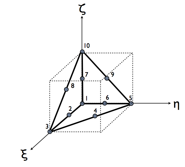
MechMonics  uses a 10-node, tetrahedral, serendipity element, as shown in Figure 1. This $C^{0}$ element provides pure quadratic interpolation of the trial and weight functions. The elements having $C^{0}$ continuity means that the trial and weight functions are continuous across (and within) elements, but their spatial derivatives are not continuous across element boundaries.

Figure 1: 10-node tetrahedral element with quadratic interpolation of the velocity, shown in the parent configuration and bounded by a unit cube.

2.5 Extraction of grain modes by singular value decomposition

The objectives of MechMonics  is to generate sets of discrete harmonic modes for every grain in a virtual polycrystal and to approximate field data using the modes in an expansion. To accomplish this, the grains must be treated separately from one another. The mesh generated by Neper  has nodal numbering globally over the entire mesh and enforces continuity of the trial and weights across the grain boundaries by having grains share nodal points on the grain boundaries. This mesh is modified In MechMonics  to introduce redundant nodes on the grain boundaries so that grains do not share nodes. Supplementary meshes are then defined for each grain using only the nodal points for that grain. This facilitates solving for the modes grain by grain.

The modes for a particular grain are the singular vectors of $\Big{[}\,\mathsf{K}\,\Big{]}$ evaluated for that grain. This in accomplished in MechMonics  with the MATLAB  function, svds, by passing it $\Big{[}\,\mathsf{K}\,\Big{]}$. Instead of using the identity matrix in Equation 9, a distributed mass matrix was computed, inverted and used to re-scale $\Big{[}\,\mathsf{K}\,\Big{]}$. This had no appreciable impact on the modes and was not incorporated in MechMonics  permanently.

2.6 Supplemental grain metrics

As previously discussed, the discrete harmonic modes are determined from Laplace’s equation applied to the grain domains. Only the grain geometry enters the formulation; there are no physical properties required. Further, no boundary conditions are applied. Consequently, the only relevant difference between the matrix equation used to determine modes for two grains within a polycrystal stems from the differences in their geometries. Because the grains can have unique geometries, the sets of modes for any given grain can be different from every other grain in the polycrystal. However, the modes do tend to share certain characteristics from grain-to-grain, as discussed in Section 3.3. To quantify the possible correlations between the modes and the geometry of a grain, a grain shape tensor [3] is computed in MechMonics. To begin, the grain centroid, $\bar{\boldsymbol{x}}$, is determined from the element centroids, $\hat{\boldsymbol{x}}$. Next, the relative position of the element centroid, $\tilde{\boldsymbol{x}}$, to the grain centroid is defined as:

$$\tilde{\boldsymbol{x}}=\hat{\boldsymbol{x}}-\bar{\boldsymbol{x}}$$ (15)

The shape tensor is computed as the weighted sum of the diads formed using the relative centroid position vectors:

$$\mathsfsl{M}=\sum_{i=1}^{m}\varphi^{i}(\tilde{\boldsymbol{x}}^{i}\times\tilde{\boldsymbol{x}}^{i})$$ (16)

where the weights, $\varphi^{i}$, are the ratios of the element volumes to the grain volume. Summation is performed over the total number of elements in the grain, $m$. The final step is to perform a singular value decompositon on $\mathsfsl{M}$. The singular vectors give the principal directions of the spatial orientation of the grain volume, referred to here as the grain axes. The singular values are the principal values, which are the squares of the grain diameters. The shape tensor is an ellipsoid whose principal values are the grain diameters.

2.7 Computational platforms

The MechMonics  source code is available at the GitHub repository: https://github.com/dplab/MechMonics. In addition to the source code, the repository contains example files and input instructions. The required input data consist solely of the output files from Neper, namely the microstructure and mesh files. Output files consist of mode data and visualization files in VTK format. MechMonics  has been developed as a MATLAB  program for use on laptop and desktop computers. Execution on other platforms with MATLAB  installed is also possible, of course. The demonstration application presented in Section 3, for example, executed on a MacBook Pro with 6 cores and 64 GB memory. (The simulations of elastoplastic responses of the sample used to generate data were performed on 64-core linux cluster using FEpX, which is a distinct code.).

3 Demonstration – Extension of FCC polycrystals

To demonstrate the application of MechMonics, the harmonic modes of three variants of one sample were computed and used to approximate the axial stress over a loading event (tensile extension to 1% nominal strain). The three variants of the sample were constructed to alter the grain morphologies, changing the uniformity of the grain size (diameter) and the uniformity of the grain sphericity. The intent is to illustrate qualitatively the sensitivity of the harmonic mode expansions to the sample instantiation. The sample variants are in some ways similar and other ways different owing to using the same starting points in their instantiations but afterward invoking constraints on grain shape and size.

In this section we discuss the Neper  instantiations of the three variants in terms of their grain diameter and grain sphericity statistics. The grain structure is presented for each sample variant along with maps of the single-crystal directional stiffness and Schmid factor defined in MechMet [5]. Mechanical attributes of the variants, evaluated using the sibling code, MechMet [5], are presented next for extensional loading. This is followed with presentation of the harmonic modes computed with MechMonicsand their associations with the grain axes. These modes are used to represent the axial stress generated with FEpX  for extension to 1% nominal strain. Attention is focused on 5 specific grains for the sample variants. For these 5 grains, both the ’raw’ (FEpX  data) and the harmonic mode expansion stress distributions are shown for several points in the loading sequence. Finally, the evolution of the mode weights are given for the 5 grains to illustrate how the stress is re-distributing through the elastic-plastic transition.

3.1 Sample instantiation and attributes

The discrete harmonic modes that are defined by the Laplace’s equation depend on the grain geometry. Samples instantiated by means of tessellations that are seeded with random points (irregularly positioned) will have dissimilar grains and thus dissimilar harmonic modes. A question that naturally arises, then, is to what extent are the modes sensitive to differences in the instantiations. The sample variants explored here were defined to exhibit distinctly different characteristics.

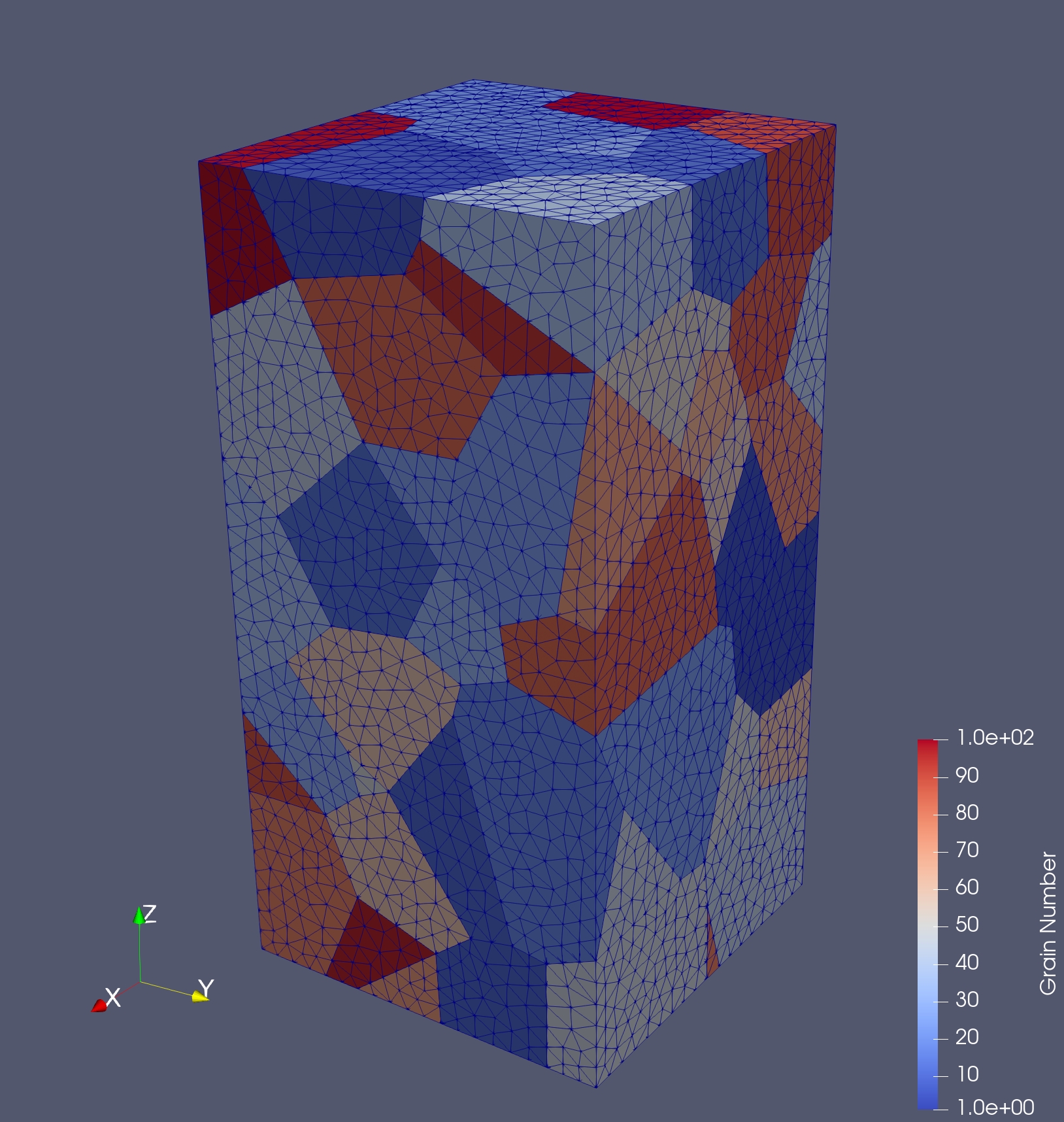
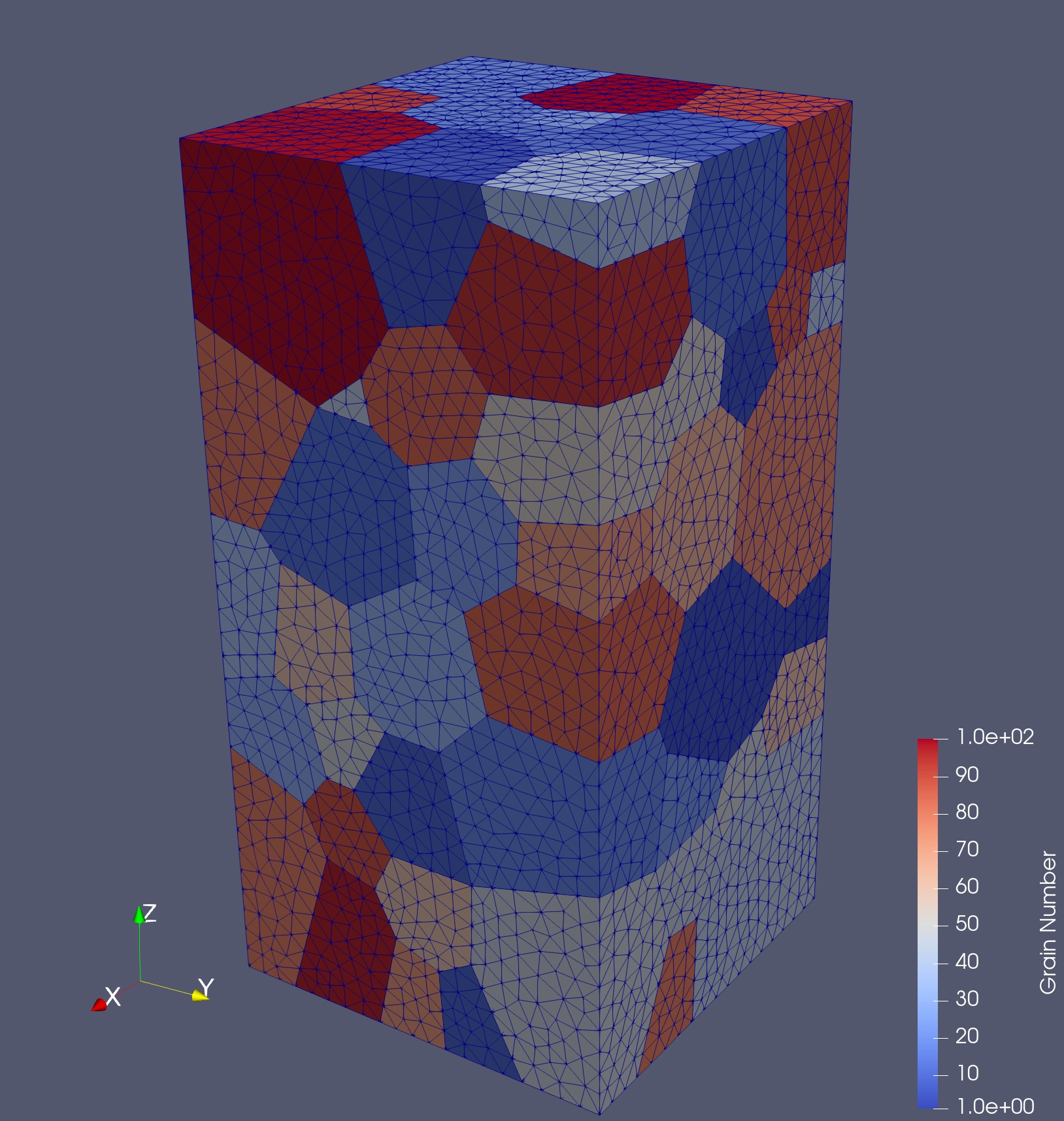
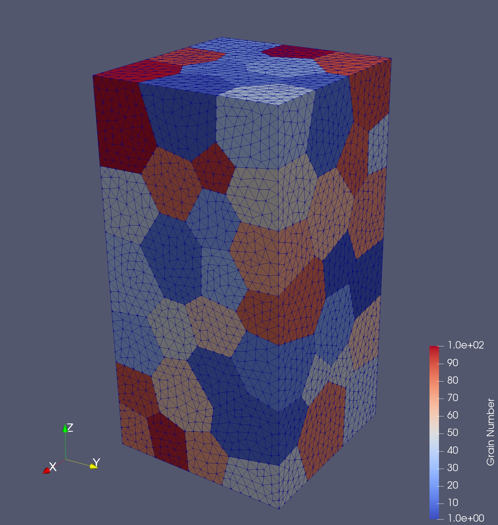
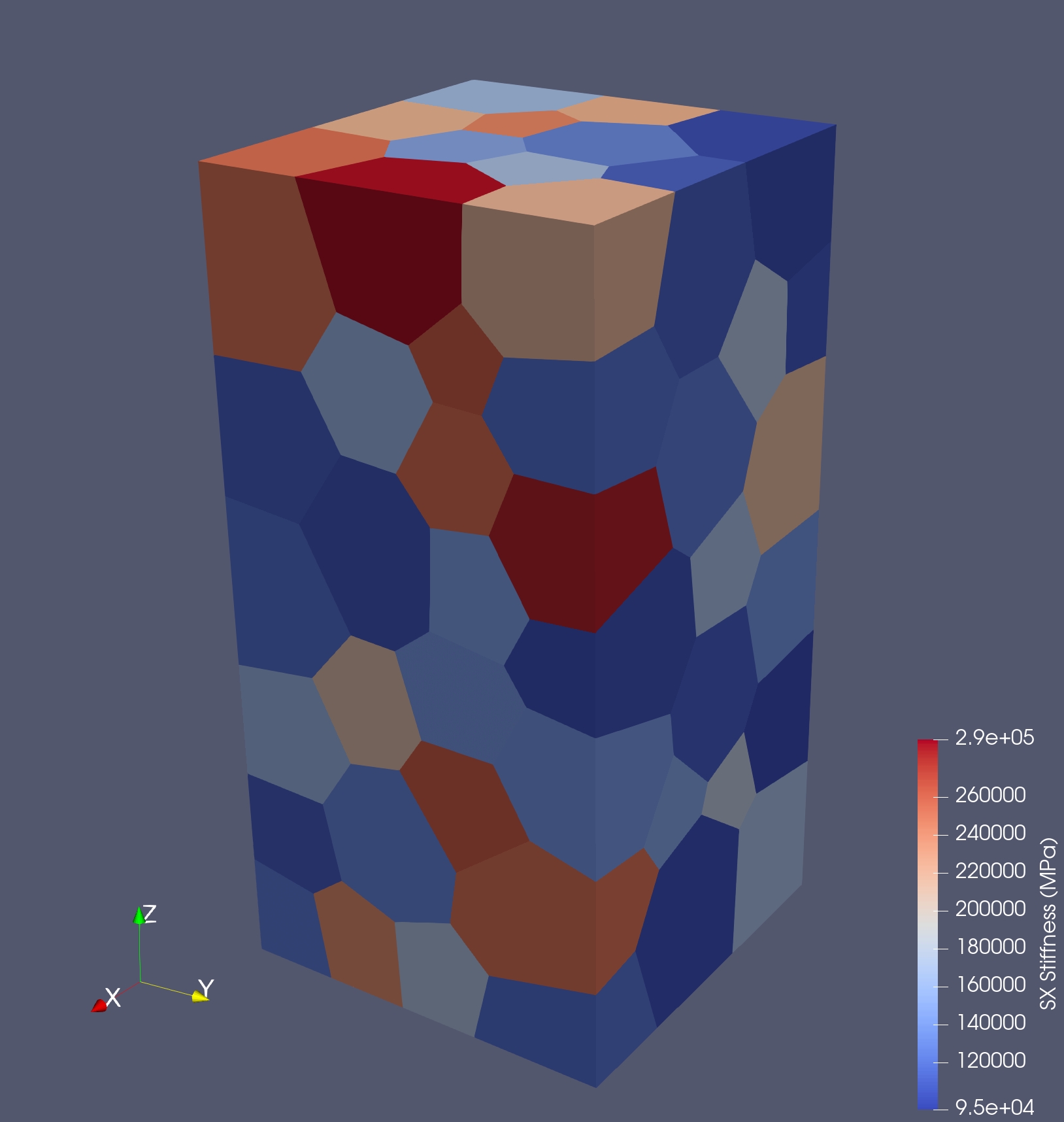
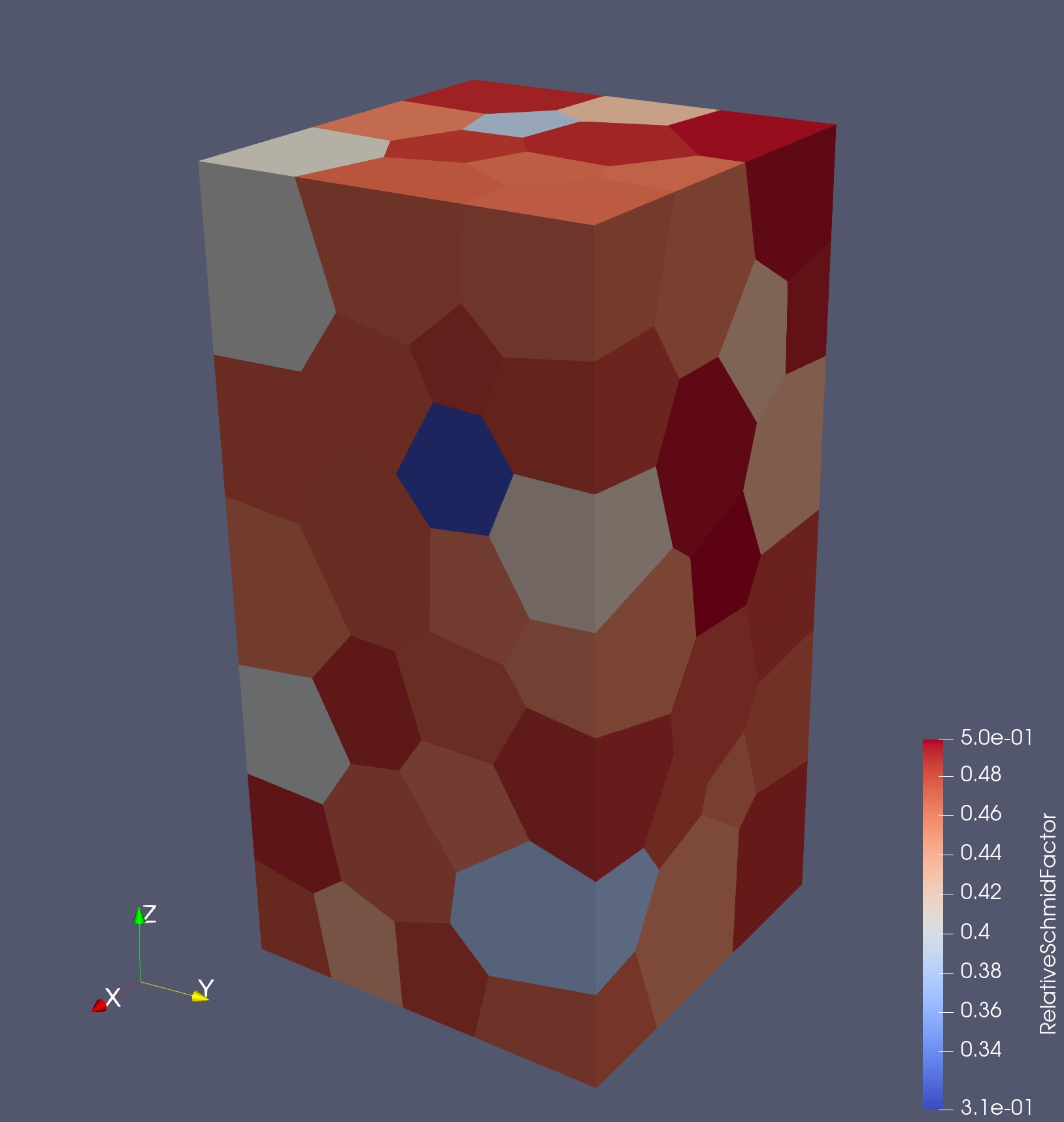
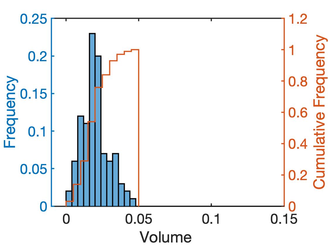
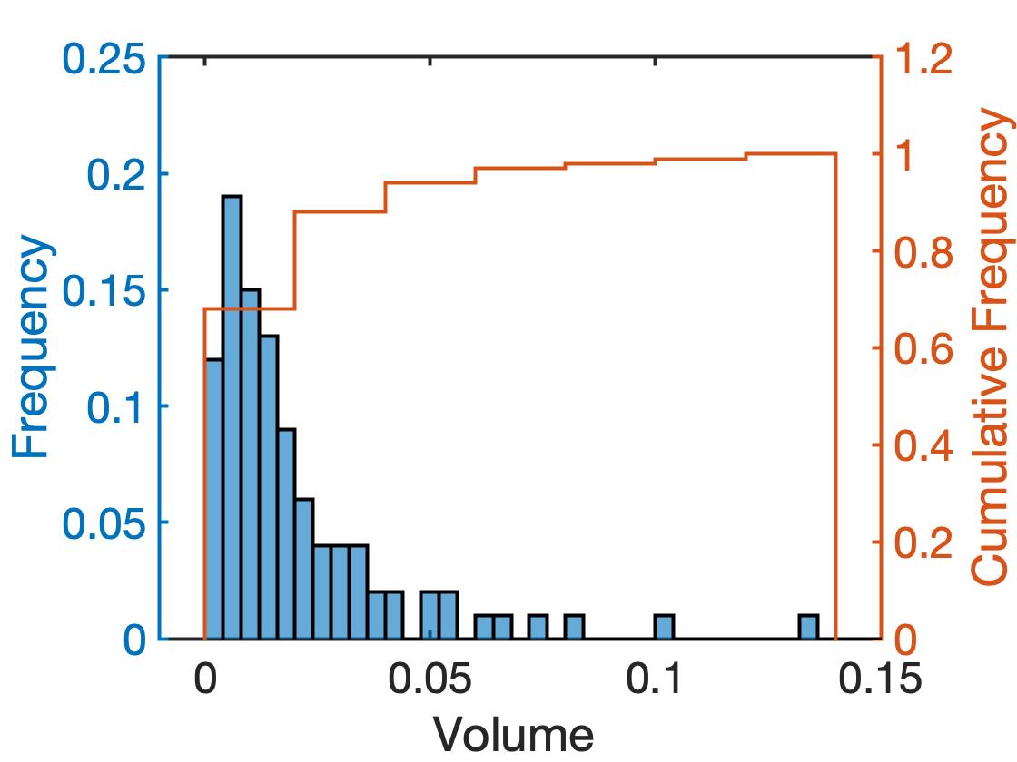
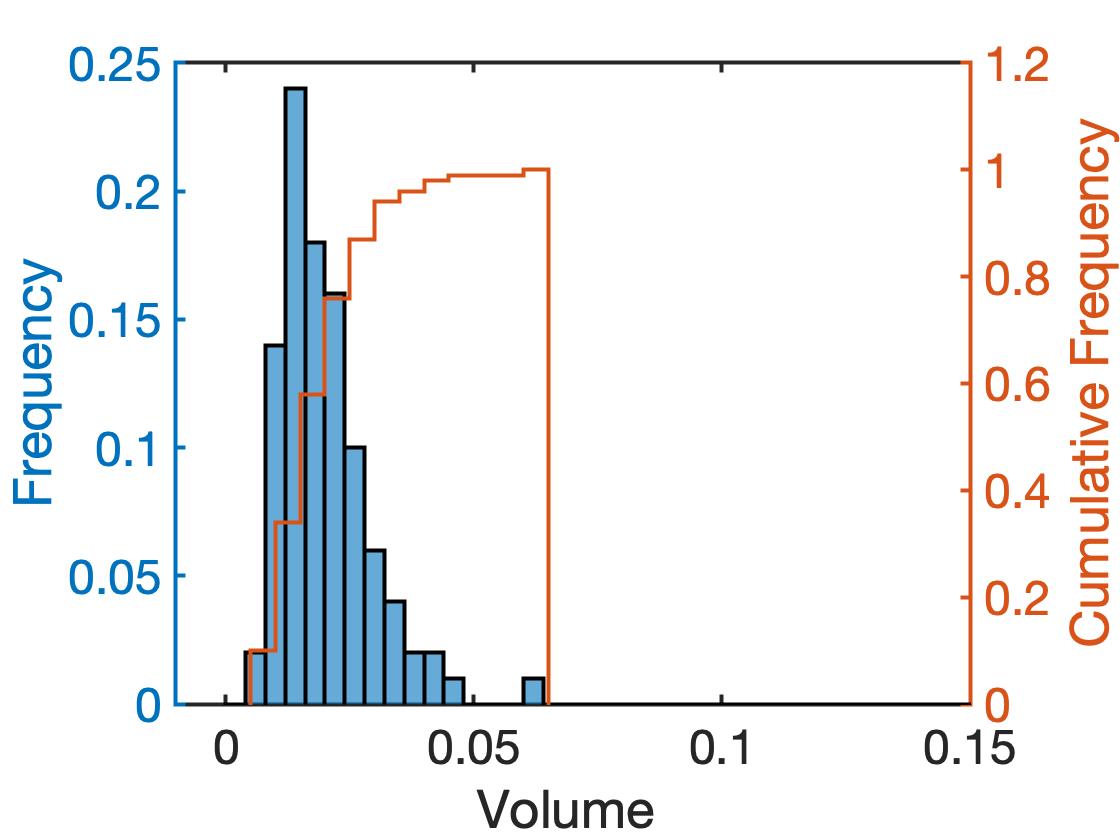
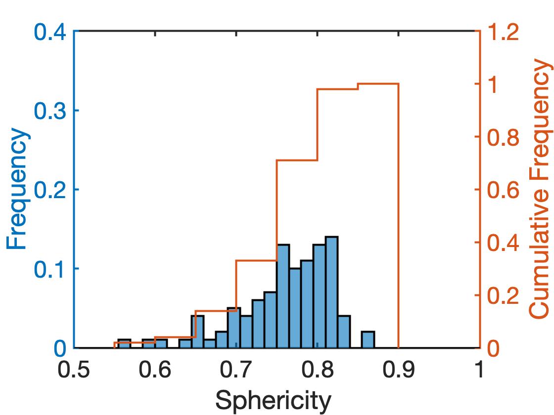
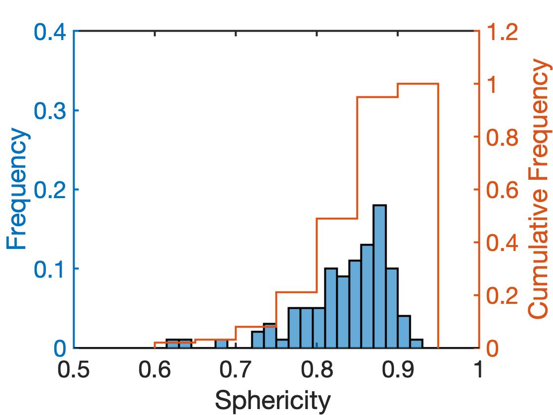
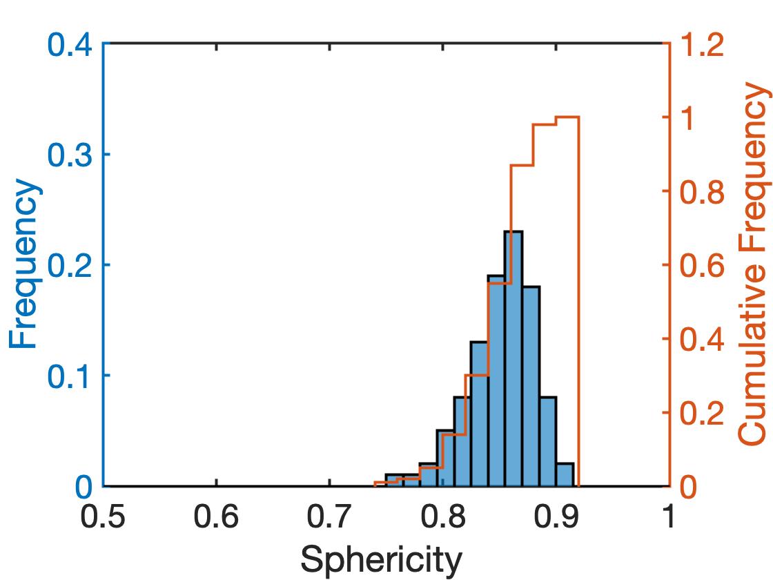
All variants were generated with Neper  and have 100 grains. All variants are Laguerre tessellations, but have been generated to have different grain morphological characteristics. In particular, tessellations were created with different grain diameter distributions and different grain sphericity distributions by altering the seed attributes (as accommodated in the Neper  input data). The three variants are shown in Figures 2, 3 and 4. Respectively, the variants are designated as (a) Voronoi, (b) Low grain size uniformity/low sphericity (LULS) and (c) high grain size uniformity/high sphericity (HUHS). The Voronoi tessellation exhibits the most irregular grain shapes. The LULS variant has more spherical grains than the Voronoi tessellation, but also has larger variations in the diameter. The HUHS variant has greater sphericity and greater size uniformity than either of the two other variants. Mean and standard deviation (SD) statistics are listed in Table 1.

	Voronoi	LULS	HUHS
Volume Mean	0.020	0.020	0.020
Volume SD	0.0092	0.0217	0.0093
Sphericity Mean	0.761	0.837	0.862
Sphericity SD	0.067	0.057	0.0287

Table 1: Diameter and sphericity statistical metrics for the three sample variants.

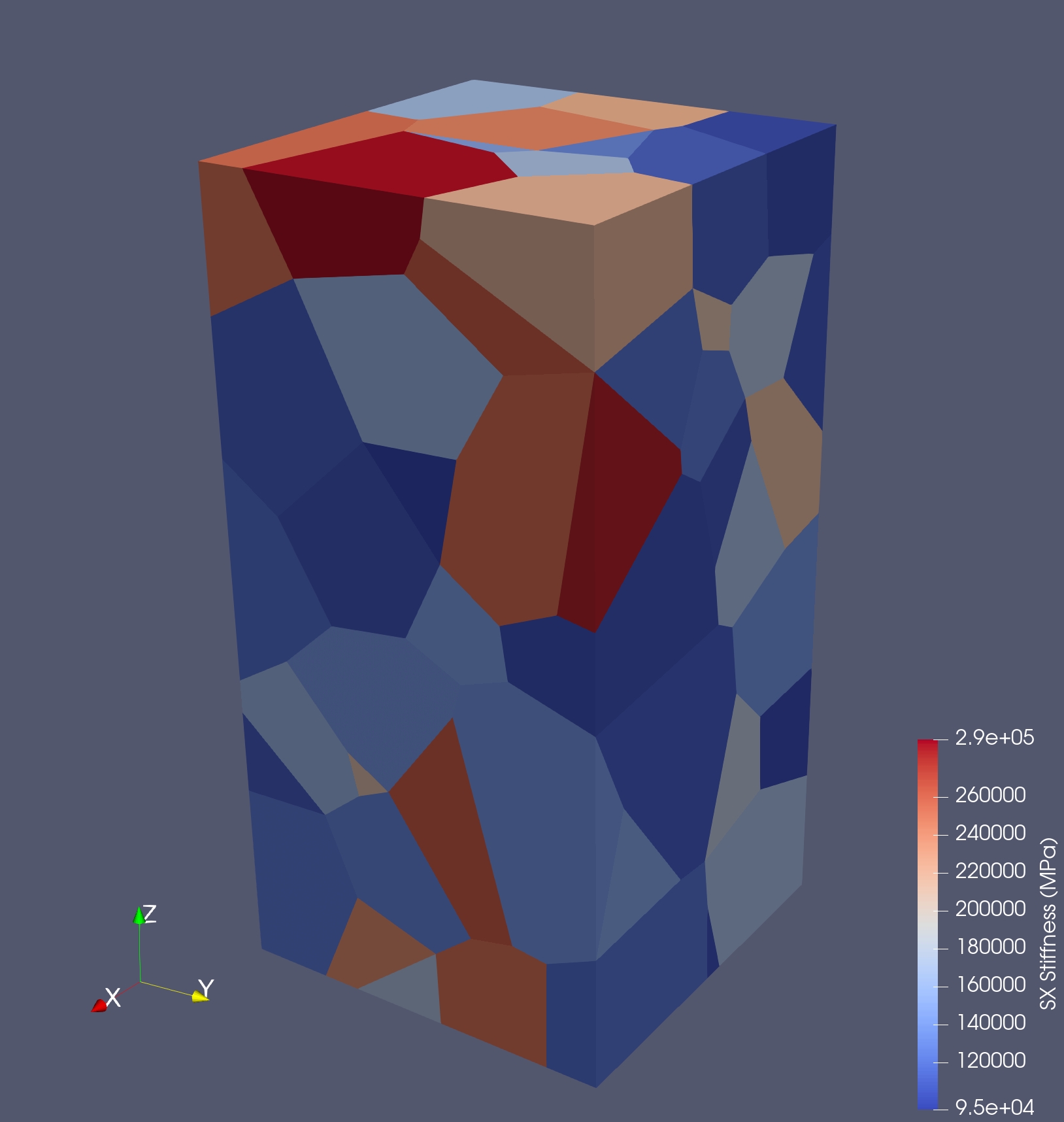
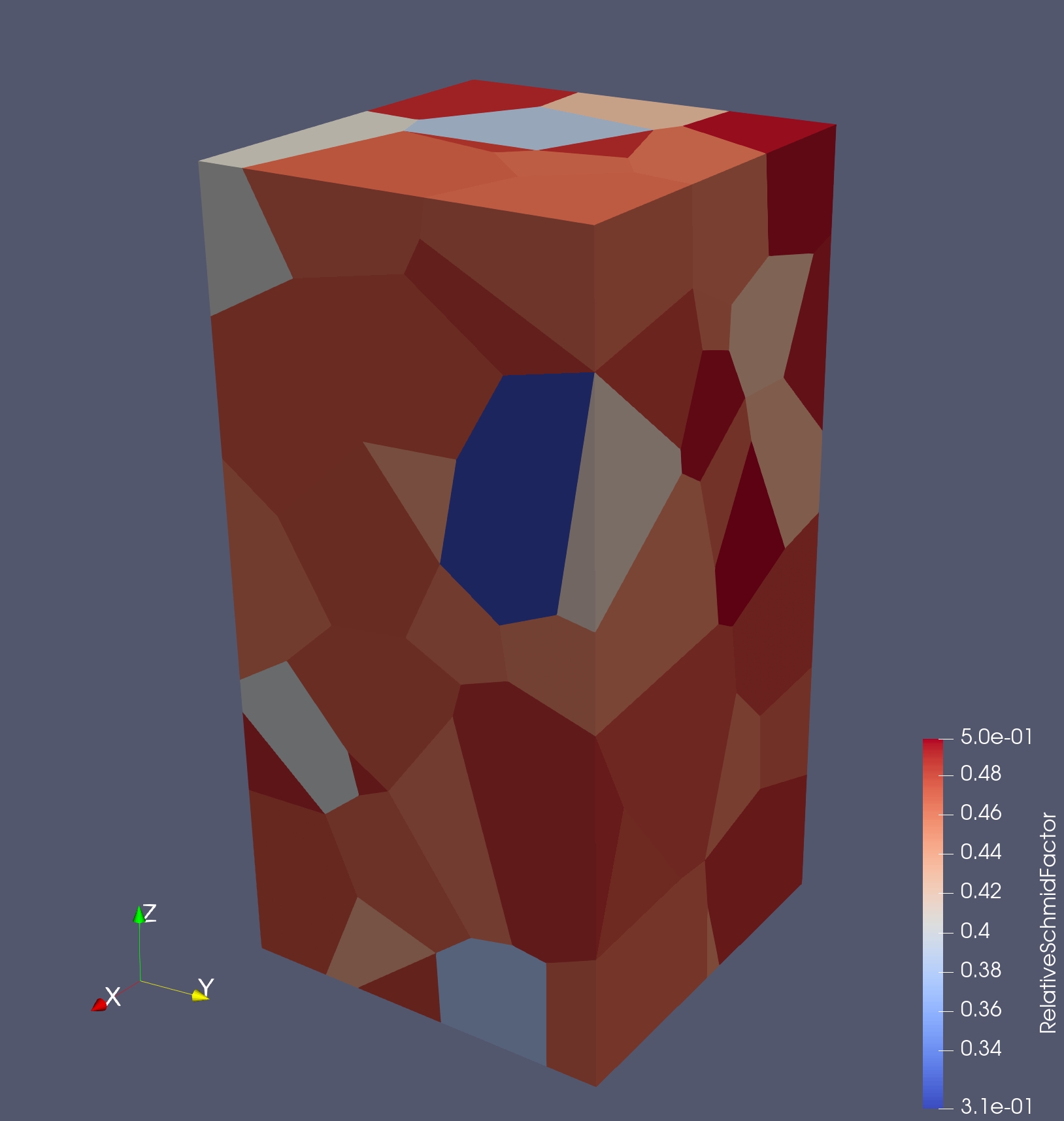
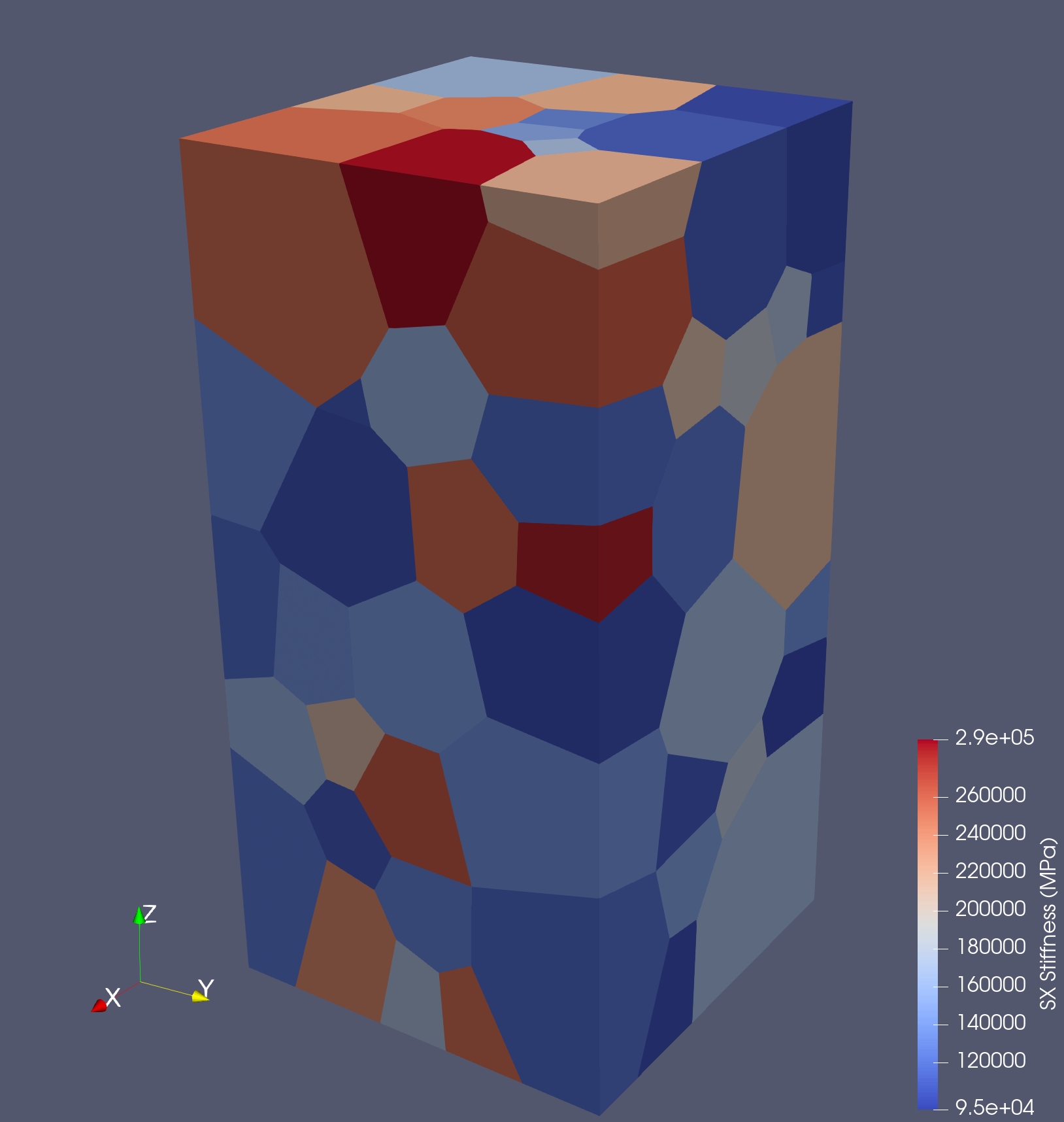
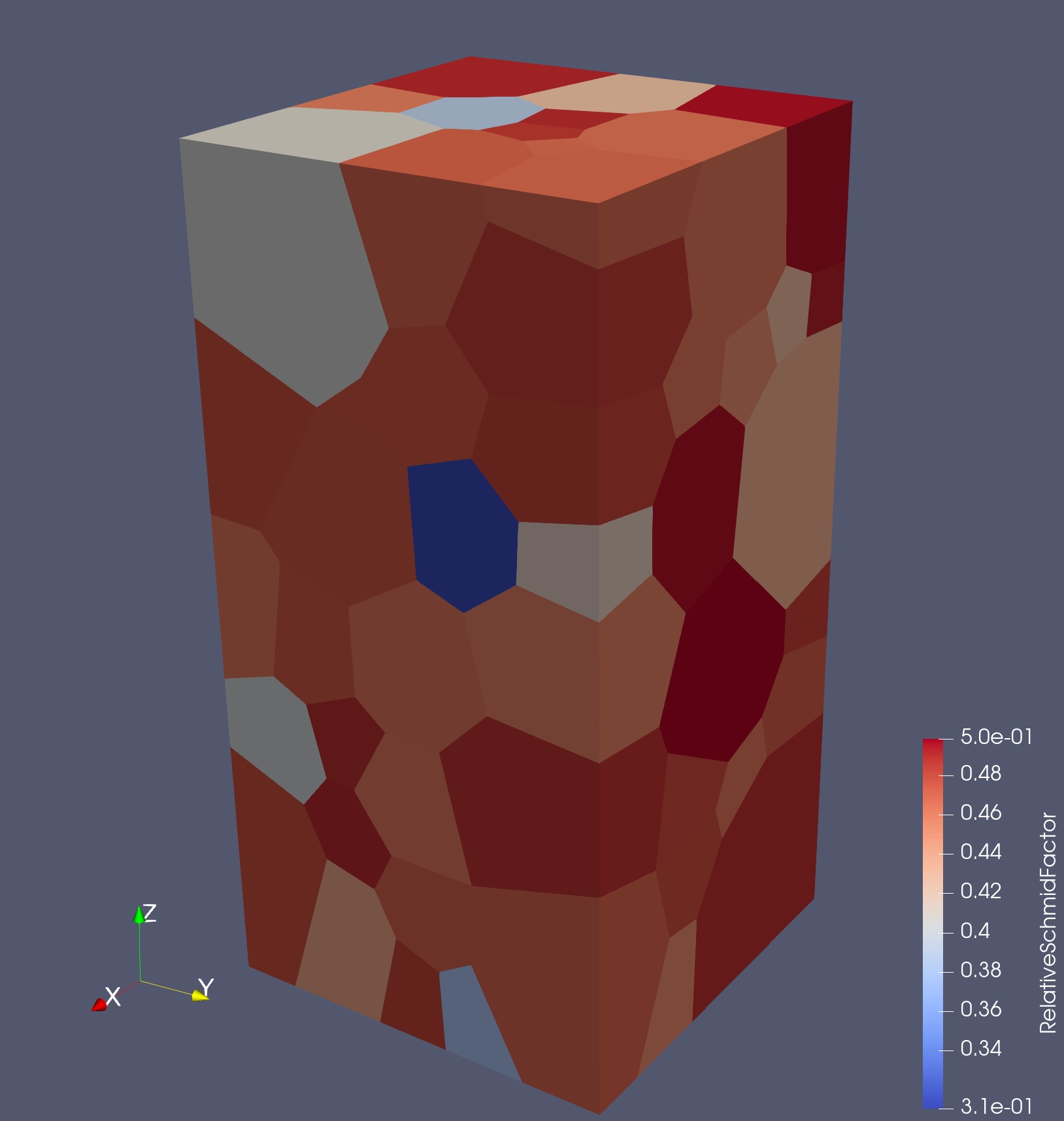
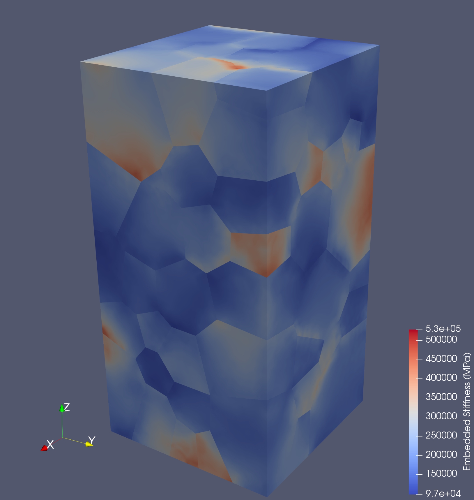
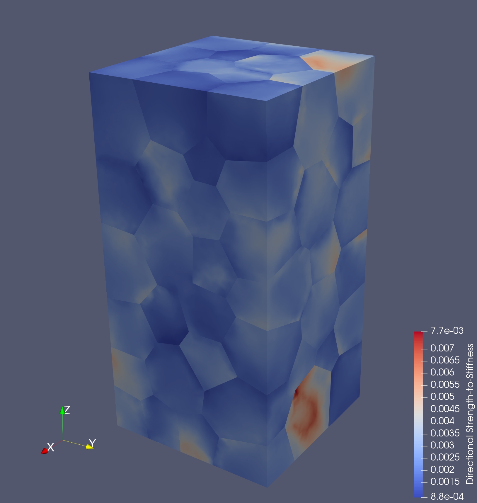
Figures 2, 3 and 4 show several aspects of the microstructures. Part(a) shows the grains with the finite element mesh. For all variants, the meshing controlled to produce virtual polycrystals with about 100K elements. Lattice orientations were assigned to the grains randomly from a uniform distribution and are uniform over the grains initially. Two single-crystal properties are shown: the z-direction (axial) directional elastic modulus (Part(b)) and the Schmid factor for z-direction (axial) tension (Part(c)), both evaluated for AL6XN [7]. In Figures 5 and 6, Two frequency distributions are shown: the grain diameter and the grain sphericity. Comparisons of these plots provide confirmation of the variant characteristics mentioned above.

(a)

(b)

(c)

Figure 2: Attributes of the Voronoi sample. (a) mesh over grains; (b) single crystal stiffness; (c) relative Schmid factor.

(a)

(b)

(c)

Figure 3: Attributes of the LULS sample. (a) mesh over grains; (b) single crystal stiffness; (c) relative Schmid factor.

(a)

(b)

(c)

Figure 4: Attributes of the HUHS sample. (a) mesh over grains; (b) single crystal stiffness; (c) relative Schmid factor.

(a)

(b)

(c)

Figure 5: Diameter frequency distributions for the sample variants (a) Voronoi; (b) LULS (c) HUHS.

(a)

(b)

(c)

Figure 6: Sphericity frequency distributions for the sample variants (a) Voronoi; (b) LULS (c) HUHS.

3.2 Sample mechanical response and mechanical metrics

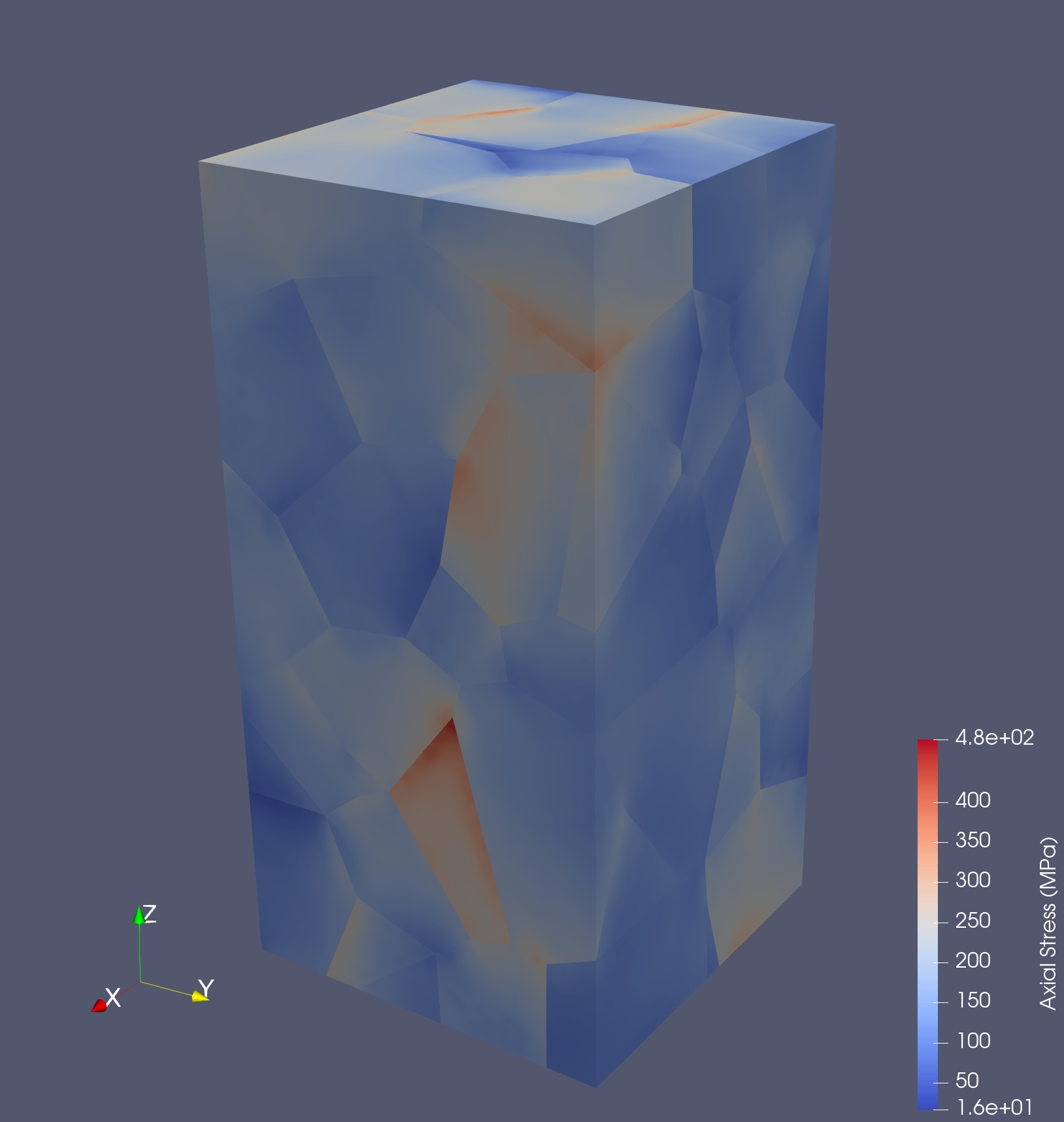
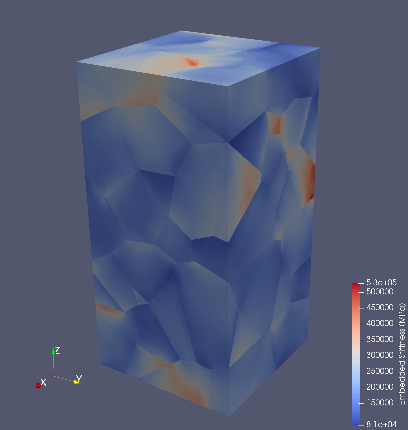
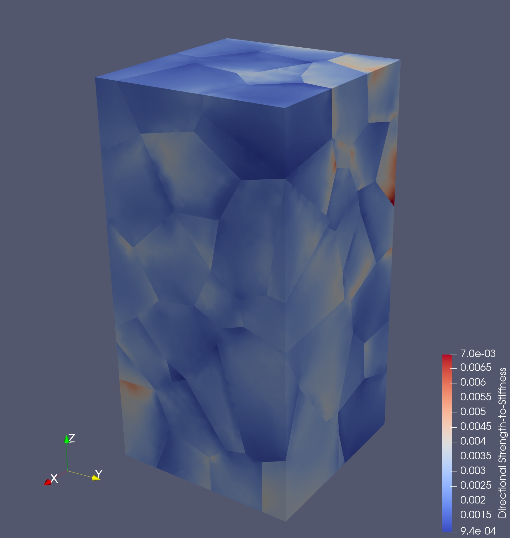
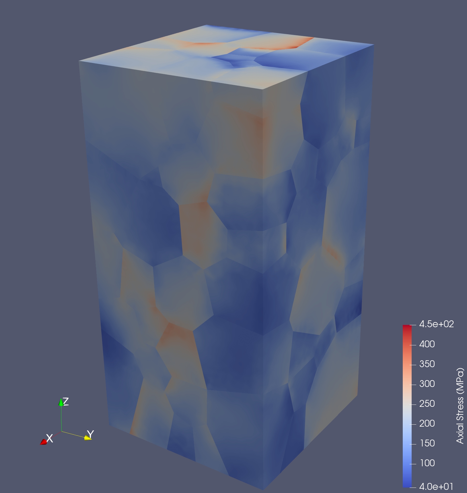
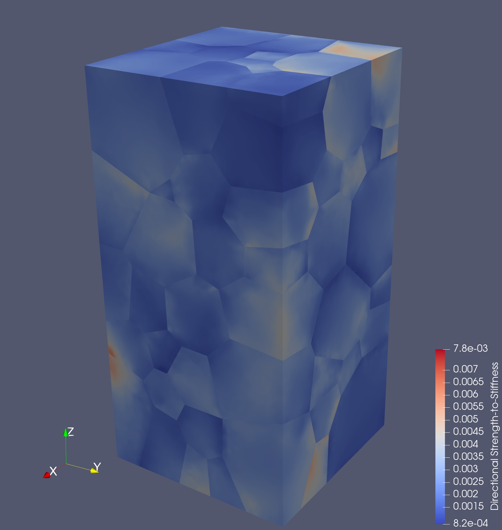
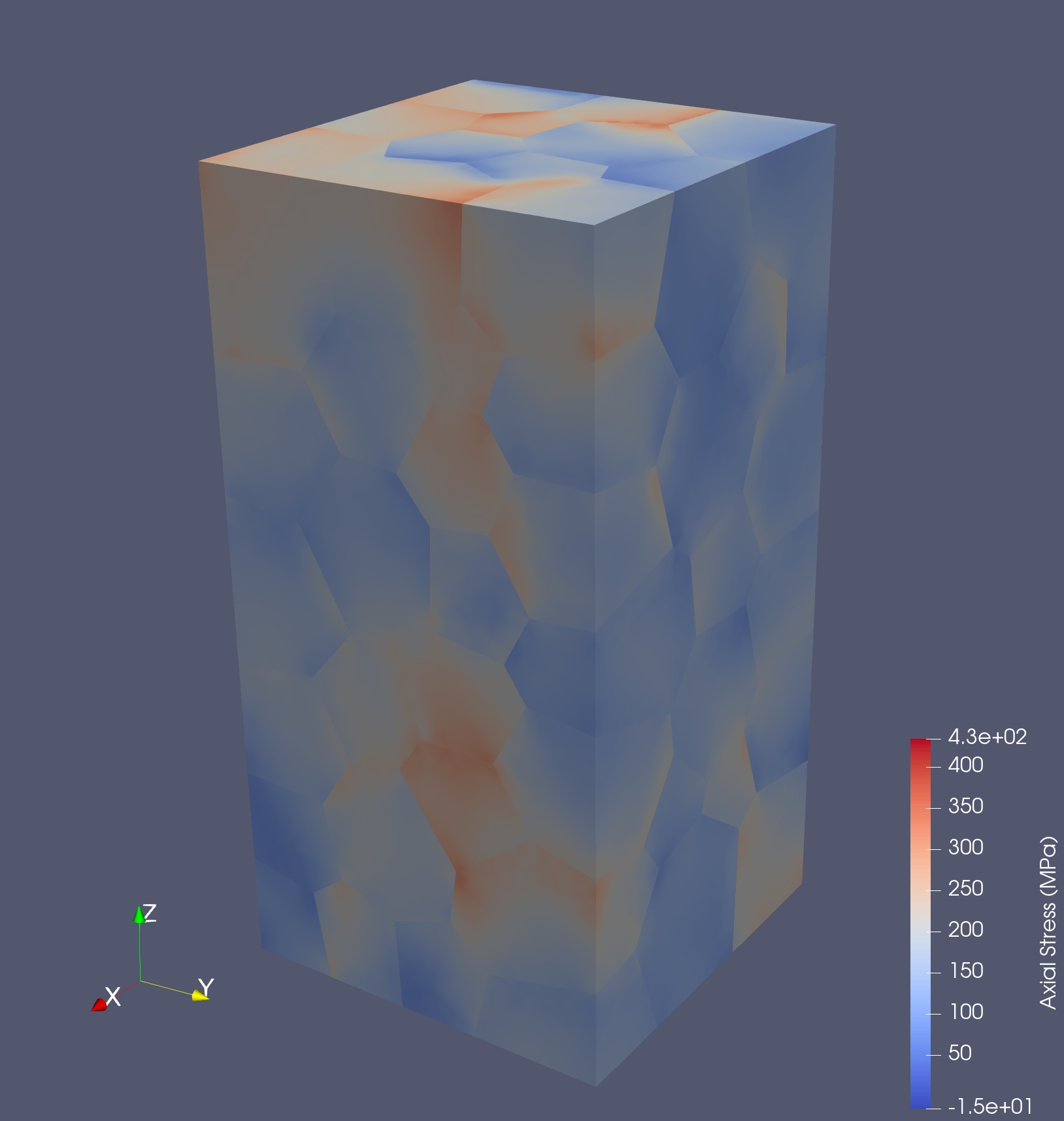
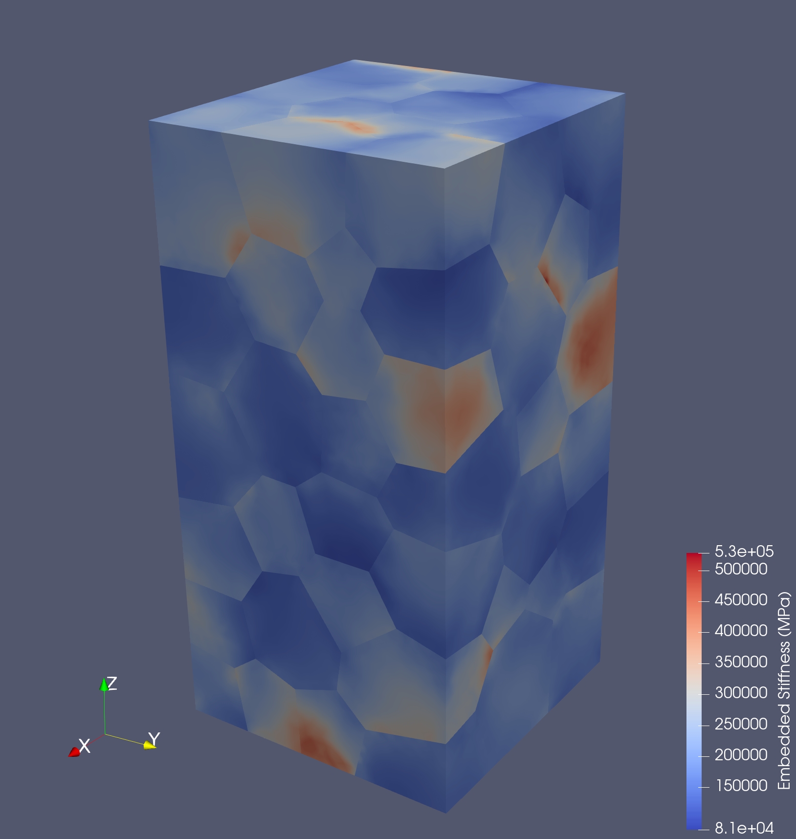
The sample variants have relatively few grains and thus might be expected to show spread in their mechanical behaviors. The mechanical characteristics of the sample variants were examined with MechMet [5] to provide insight in this regard. The single-crystal elastic moduli correspond to AL6XN [7]. Figures 7, 8 and 9 give information for the Voronoi, LULS and HUHS sample variants, respectively. Part (a) of each figure shows the axial stress distribution for 0.1% extensional strain in the $z$ coordinate direction. Spatial variations in the stress are evident; these arise in a grain within an anisotropic polycrystals from the influence of its neighbors on the loading. Embedded (apparent) stiffness is shown in Part (b), and can be compared to the single-crystal directional stiffness distributions shown in Part (b) of Figures 2, 3 and 4. Variations within grains exist due to intra-grain deformation heterogeneities associated with neighborhood effects. The directional strength-to-stiffness ratios quantify the influence of stiffness on onset of yielding as well as neighborhood affects. Distributions of strength-to-stiffness are provided in Part (c). One can say that there appear to exist trends in all these (related) fields that are shared across the sample variants. However, the grain morphologies do play a substantial role in the location of extreme values of the fields. This has a bearing on the activation of modes, particularly higher modes, in the representation of data.

(a)

(b)

(c)

Figure 7: Mechanical metrics of the Voronoi sample. (a) axial stress; (b) embedded stiffness; (c) directional strength-to-stiffness ratio.

(a)

(b)

(c)

Figure 8: Mechanical metrics of the LULS sample. (a) axial stress; (b) embedded stiffness; (c) directional strength-to-stiffness ratio.

(a)

(b)

(c)

Figure 9: Mechanical metrics of the HUHS sample. (a) axial stress; (b) embedded stiffness; (c) directional strength-to-stiffness ratio.

3.3 Harmonic modes

For the three sample variants, discrete harmonic modes were determined with MechMonics  according to the approach laid out in Section 2. For the demonstration objectives here, only the first 10 modes are discussed. To represent the stress distribution computed in FEpX  with error levels below 1% would require 20-30 modes based on experience to date. This is a reflection of the real complexity of stress distributions in polycrystals that have complicated grain morphologies and anisotropic properties. Modes 2, 5 and 9 are shown for each sample in Figures 10, 11 and 12.

(a)

(b)

(c)

Figure 10: Harmonic modes of the Voronoi sample. (a) Mode 2; (b) Mode 5; (c) Mode 9.

(a)

(b)

(c)

Figure 11: Harmonic modes of the LULS sample. (a) Mode 2; (b) Mode 5; (c) Mode 9.

(a)

(b)

(c)

Figure 12: Harmonic modes of the HUHS sample. (a) Mode 2; (b) Mode 5; (c) Mode 9.

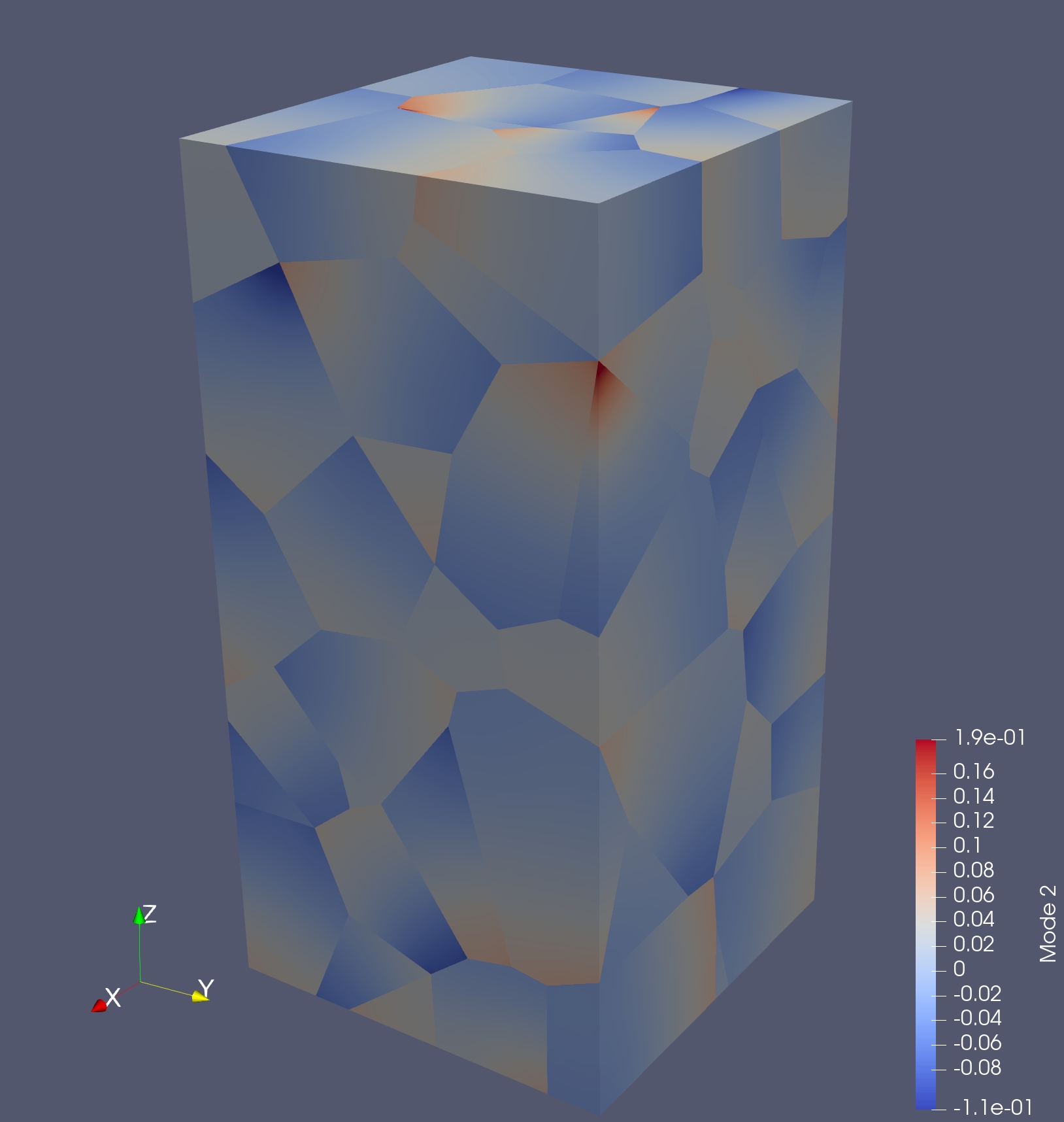
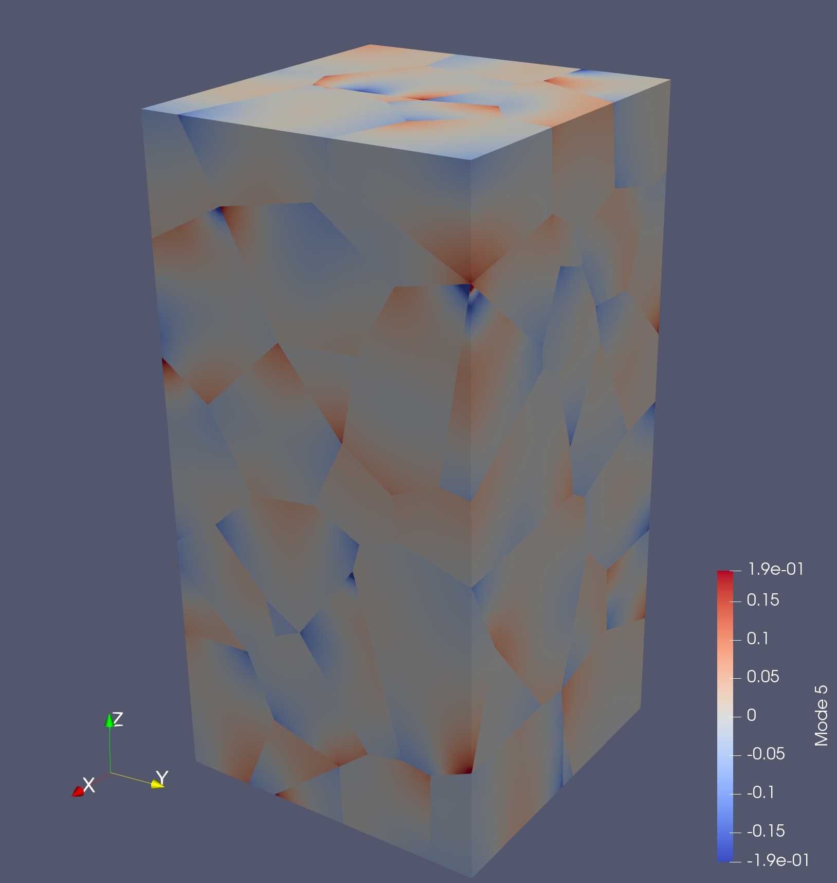
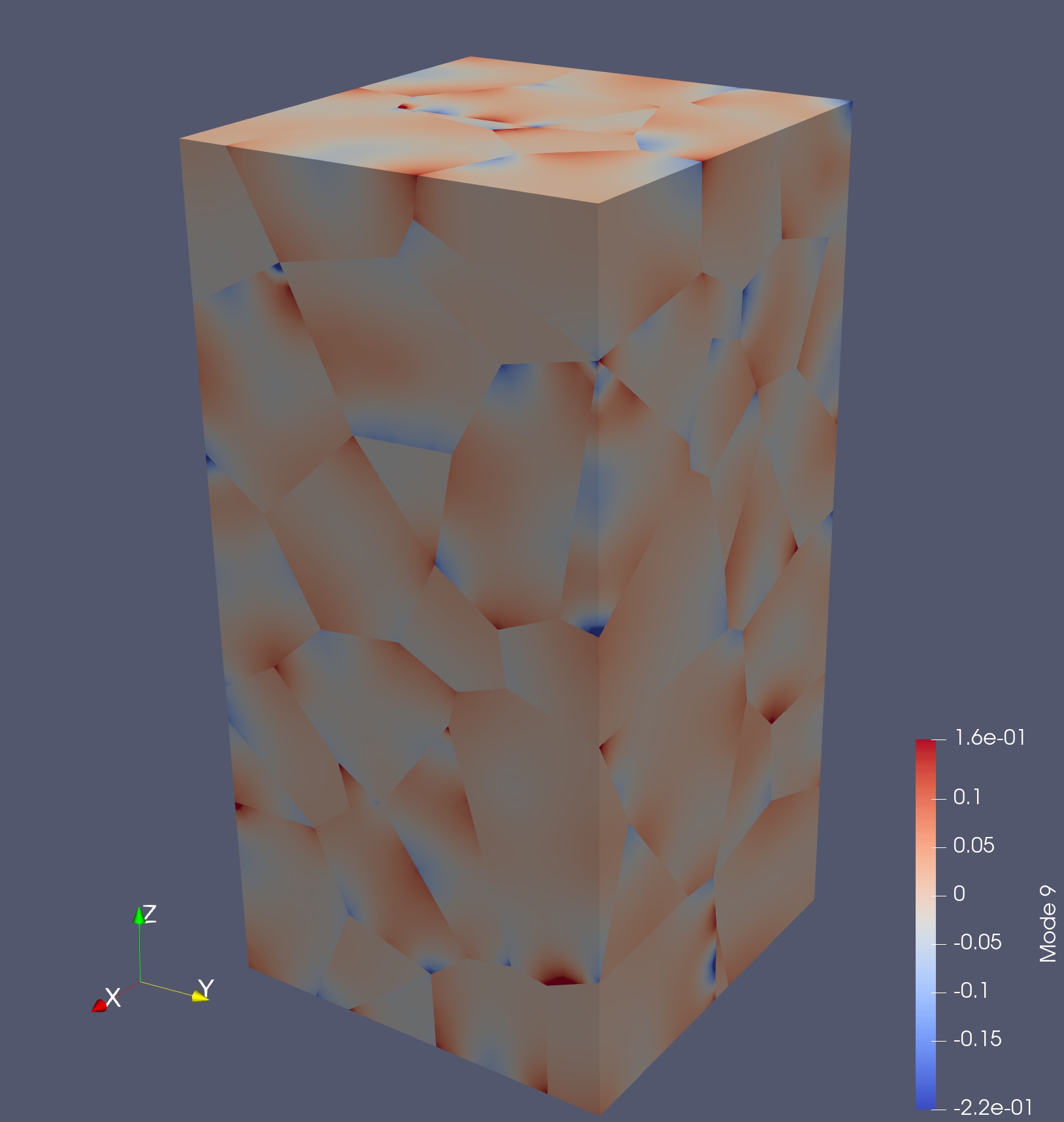
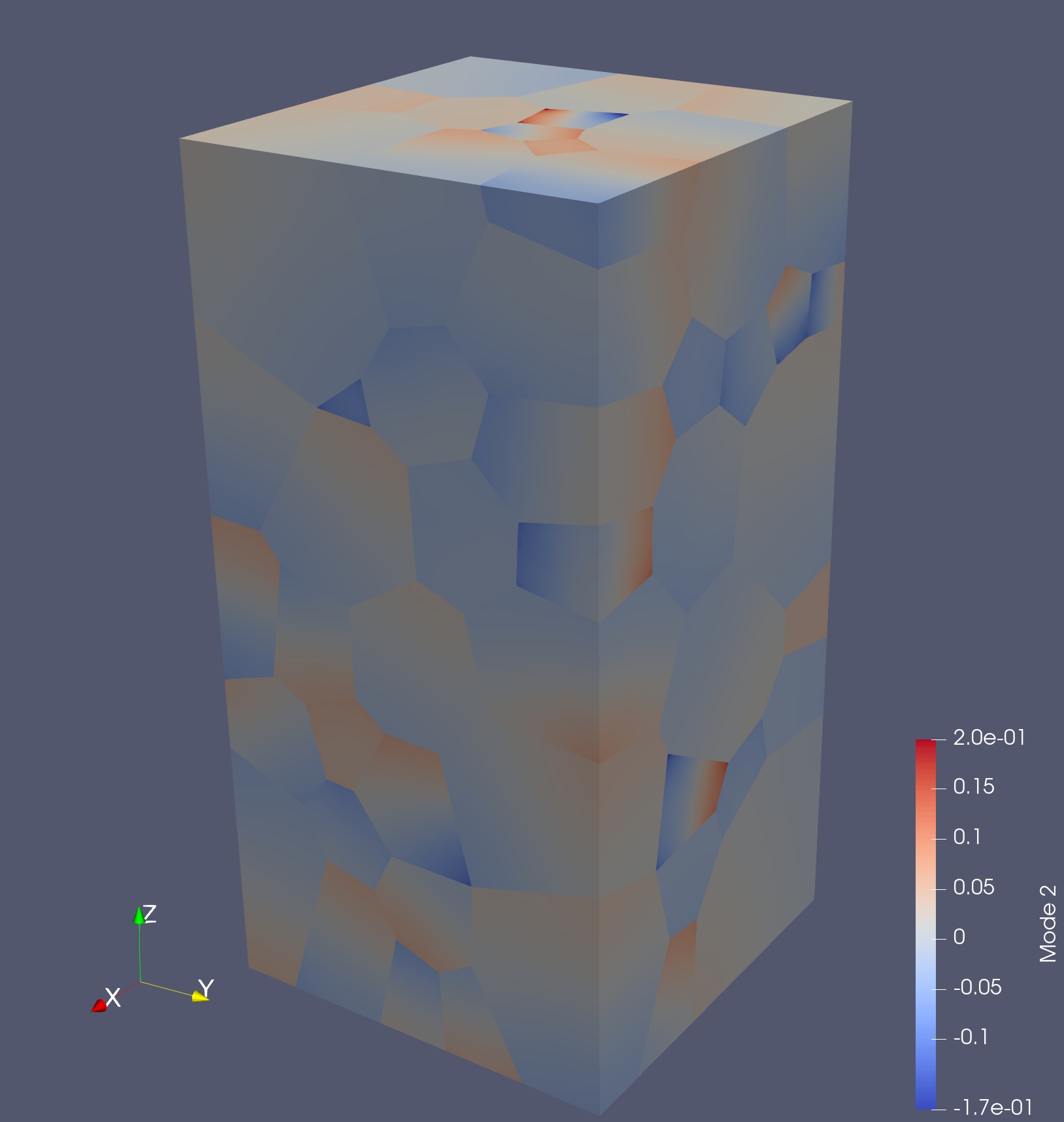
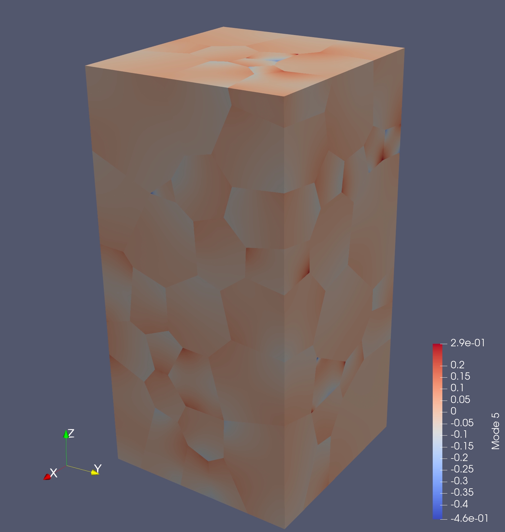
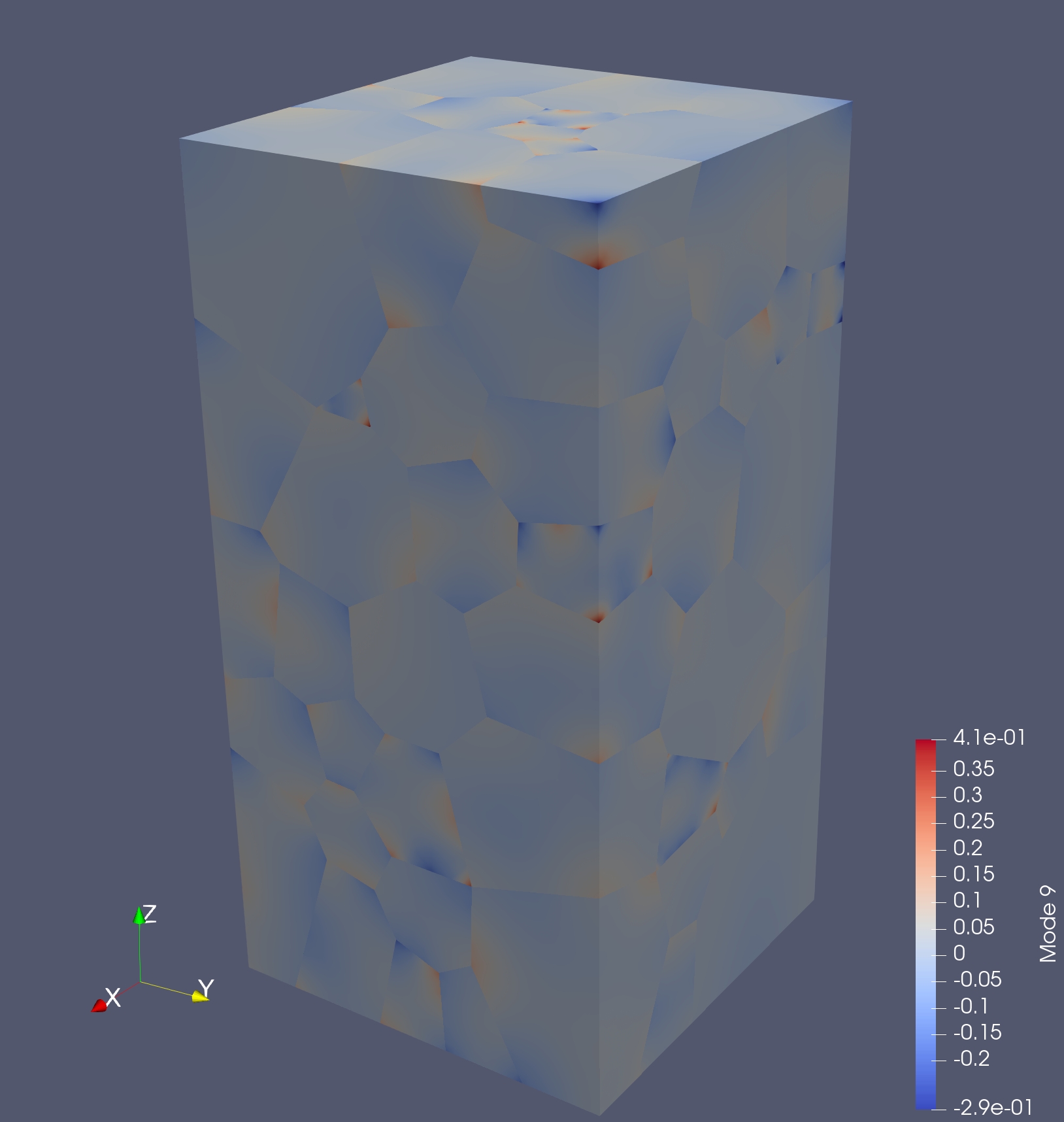
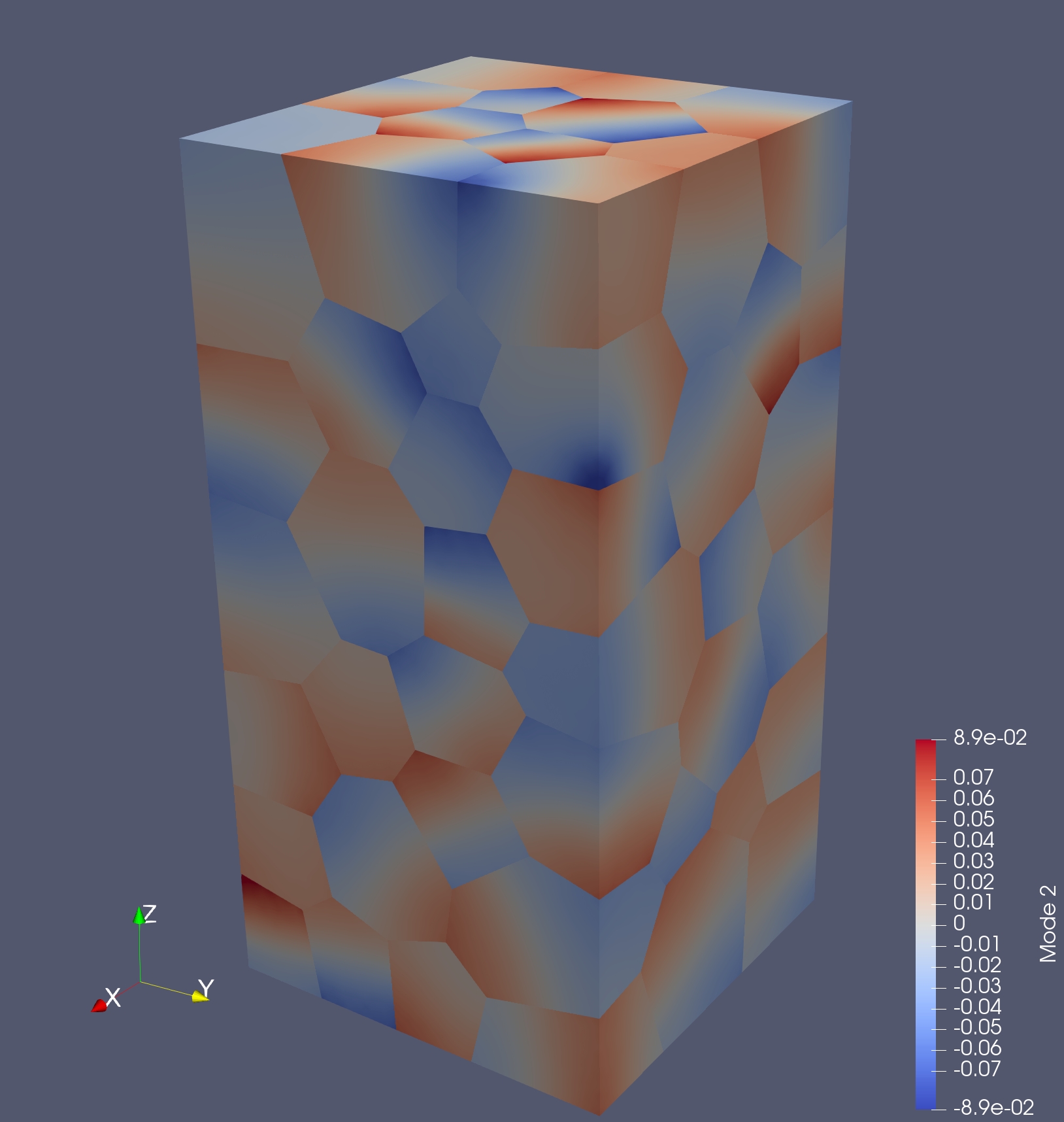
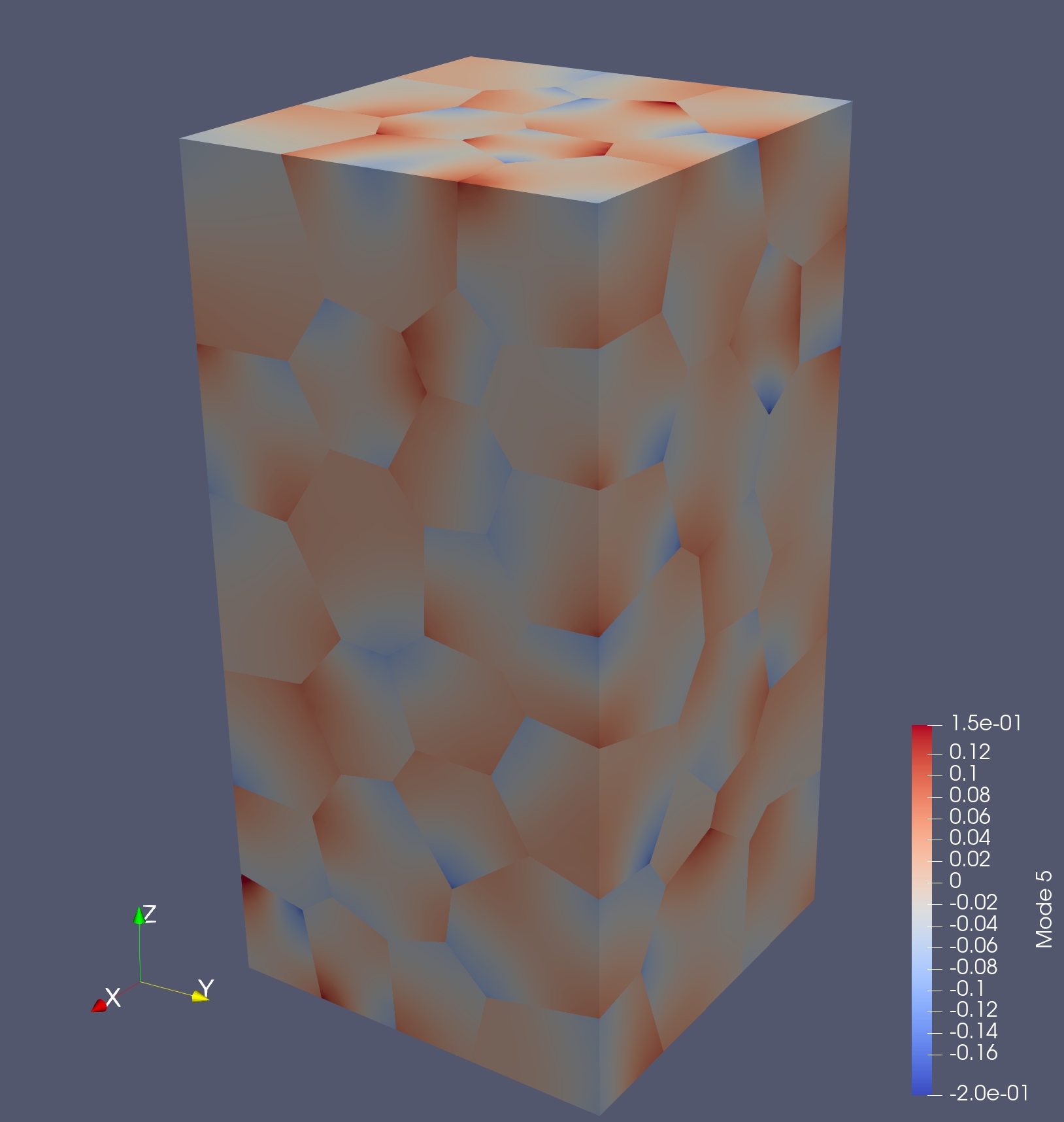
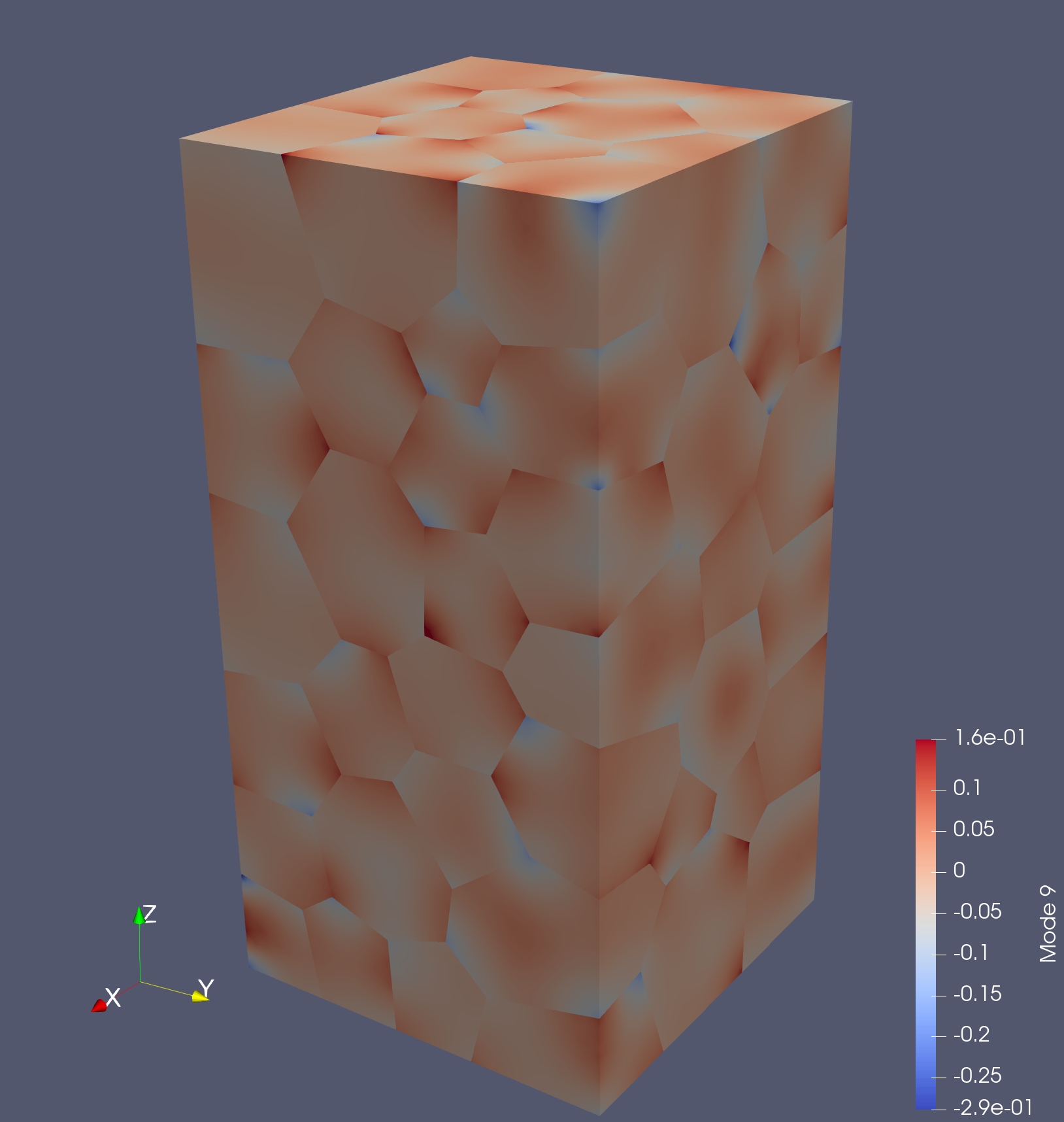
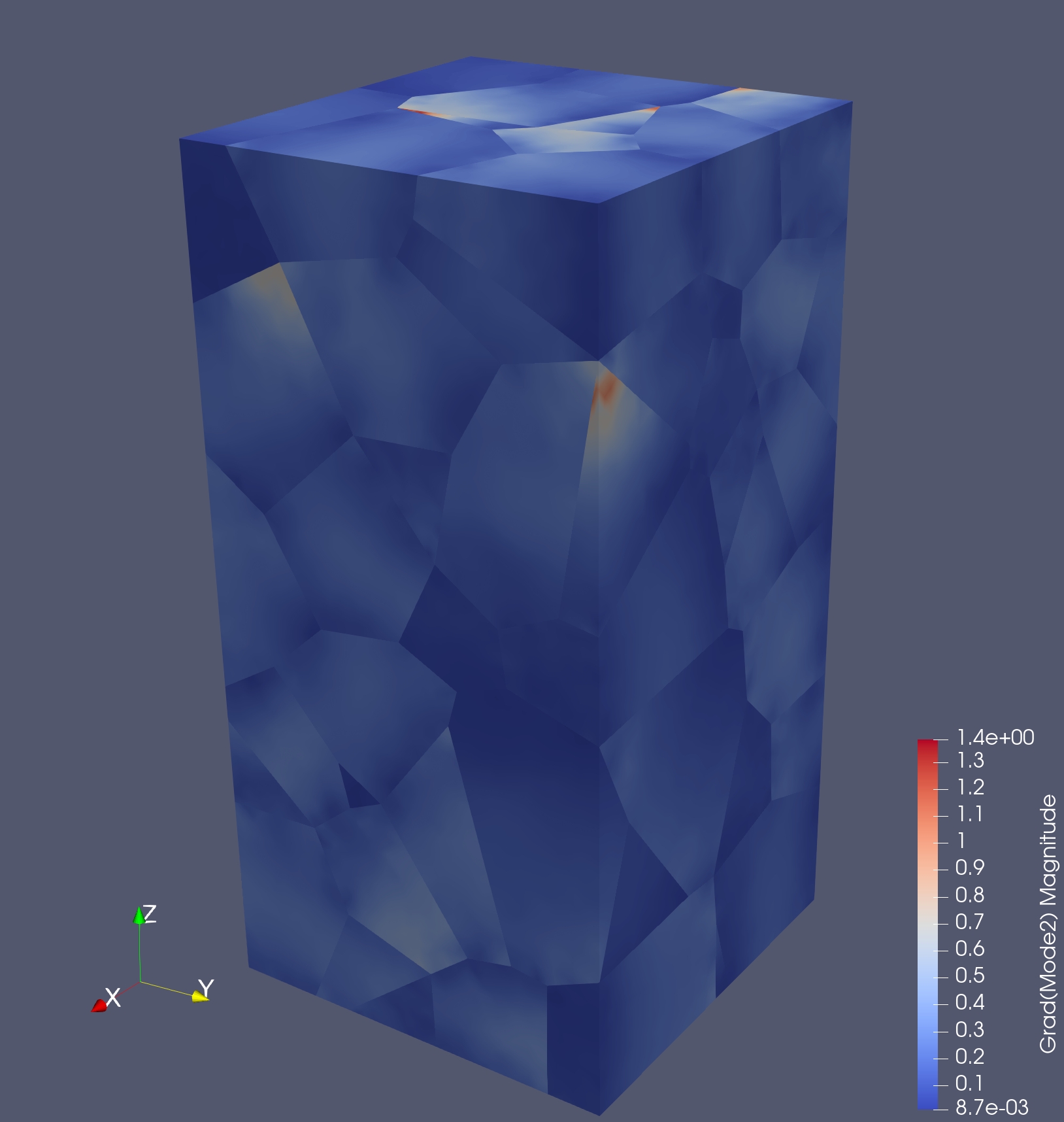
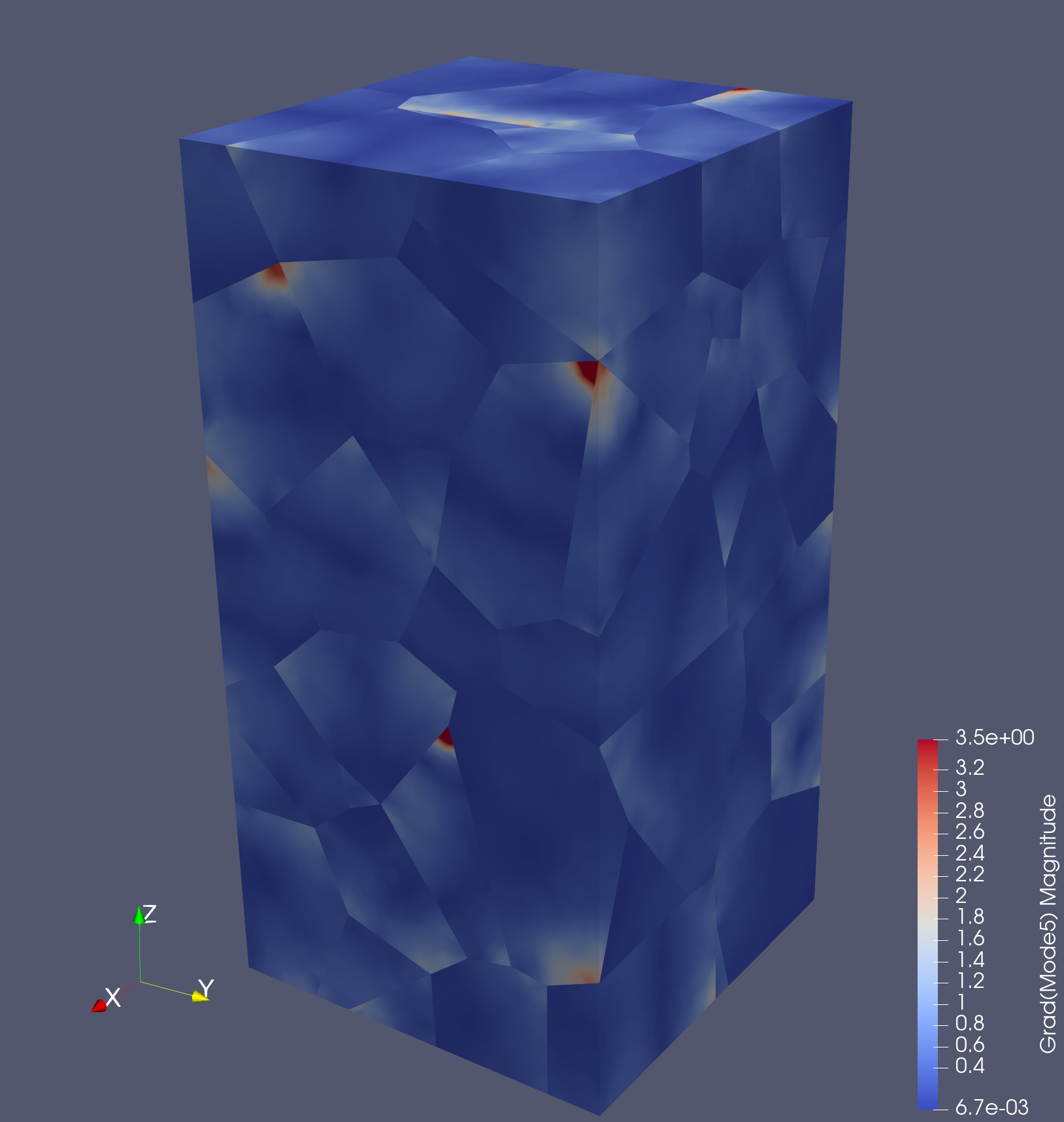
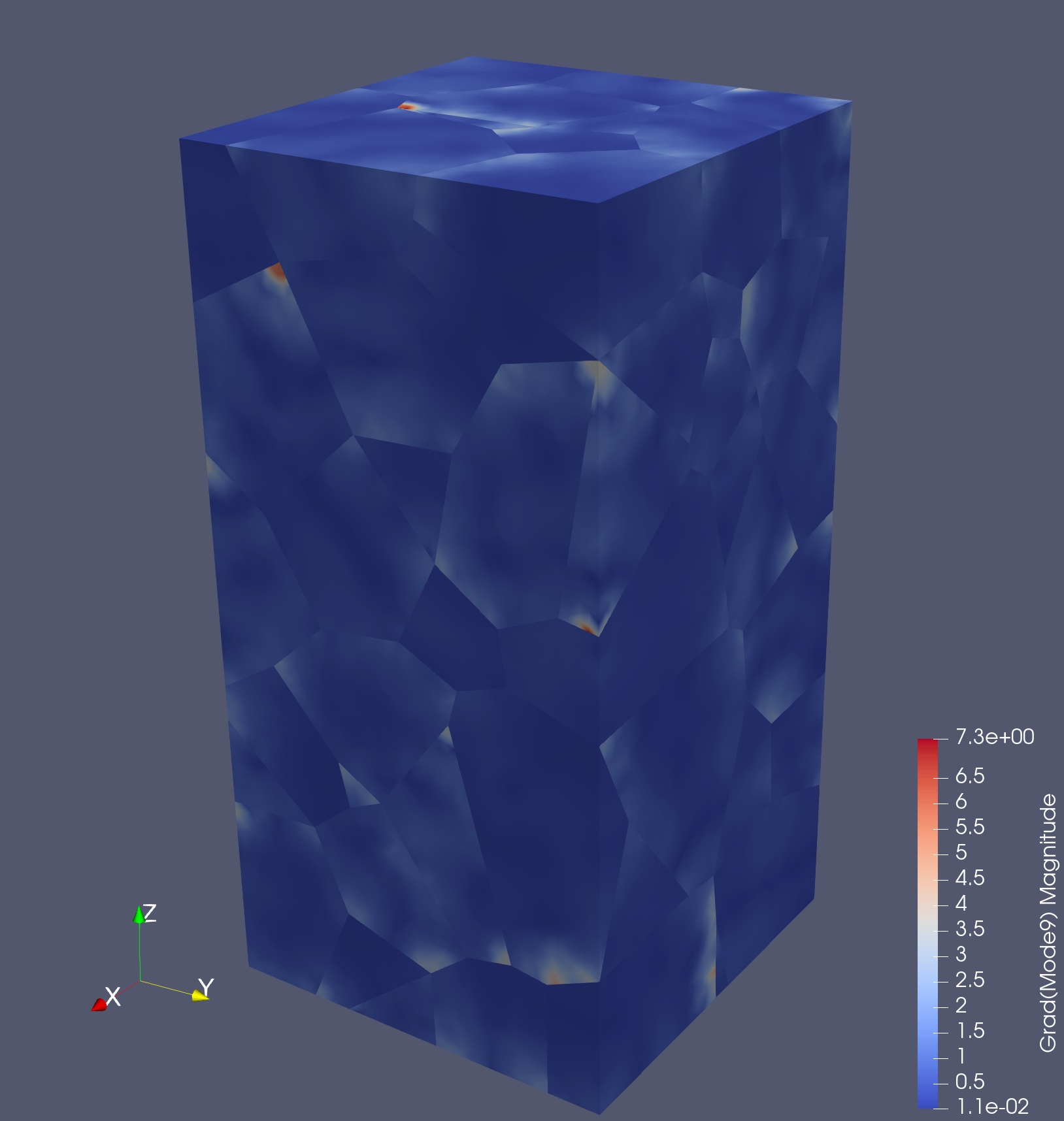
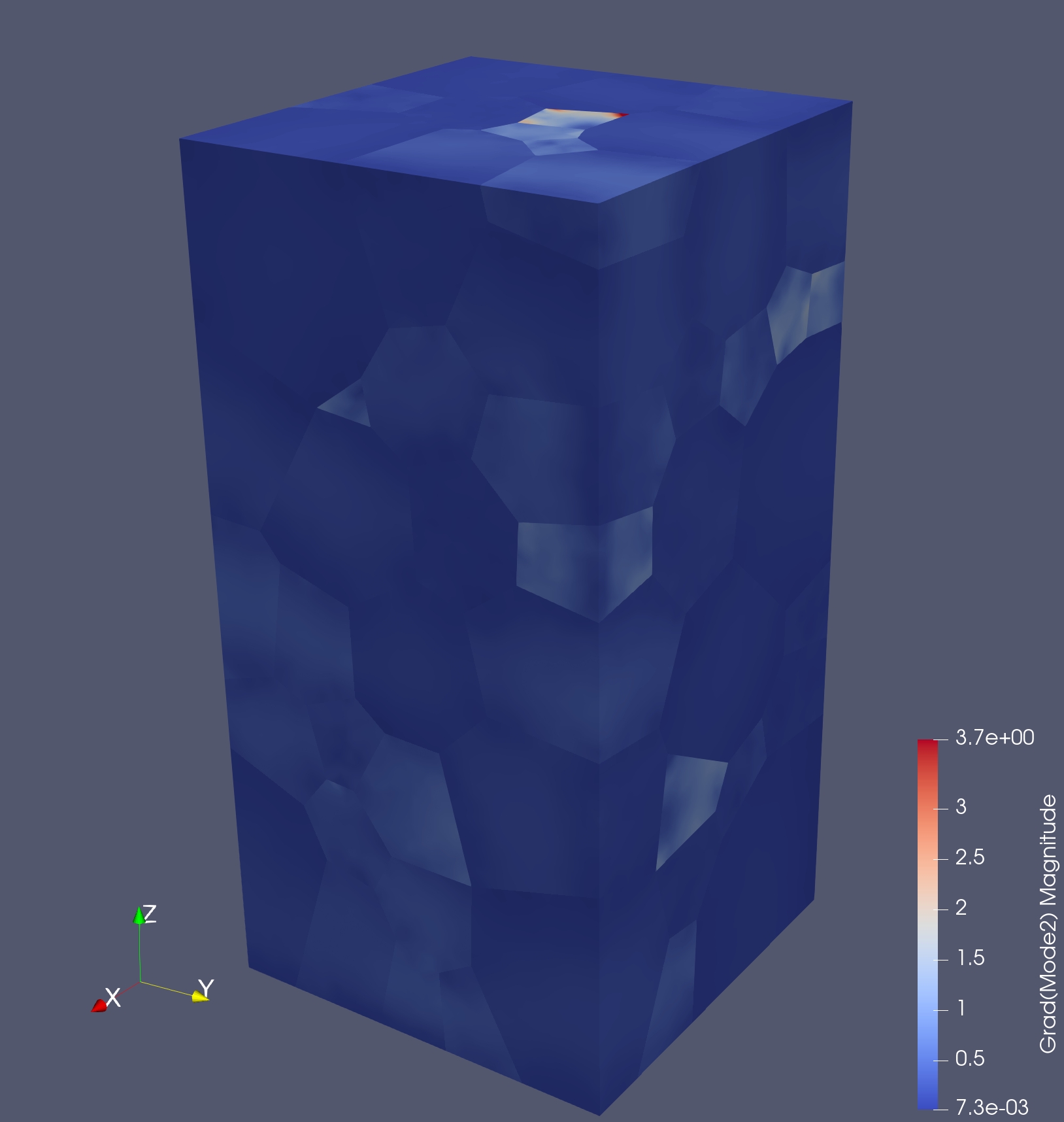
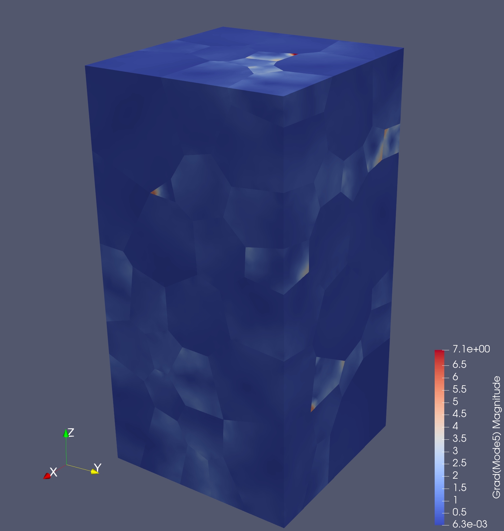
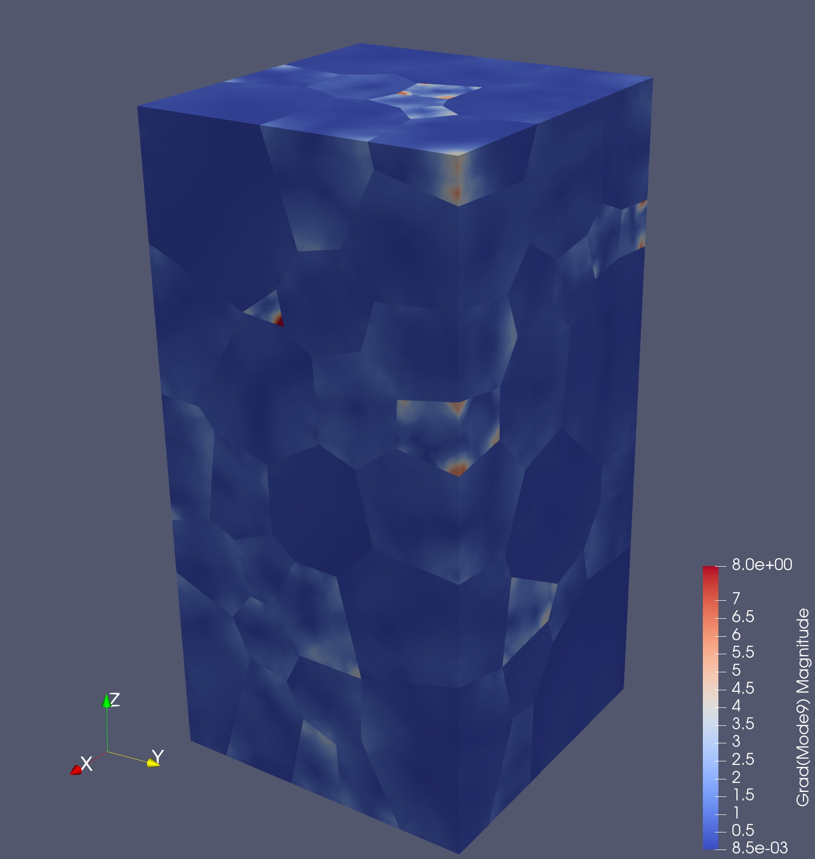
First, Mode 1 (not shown) is the constant mode for each set of harmonic modes. Modes 2 to 10 are not constant, but rather vary over the grain with increased complexity as the mode number increases. Mode 2 has monotonically increasing or decreasing distributions. However, its gradients are not constants (so the mode is not linear). Generally speaking, the values of the gradient of Mode 2 are lower than corresponding values for the other modes. Modes 5 and 9 have more complex distributions and definitely are not monotonic over grains. Note that in general the mode patterns do not repeat the same pattern from grain to grain. Rather, each grain has its own unique set of modes owing to its unique size and shape. Similarities among the modes appears to be the greatest for HUHS and the lowest for LULS, but this observation is made without quantitative analysis.

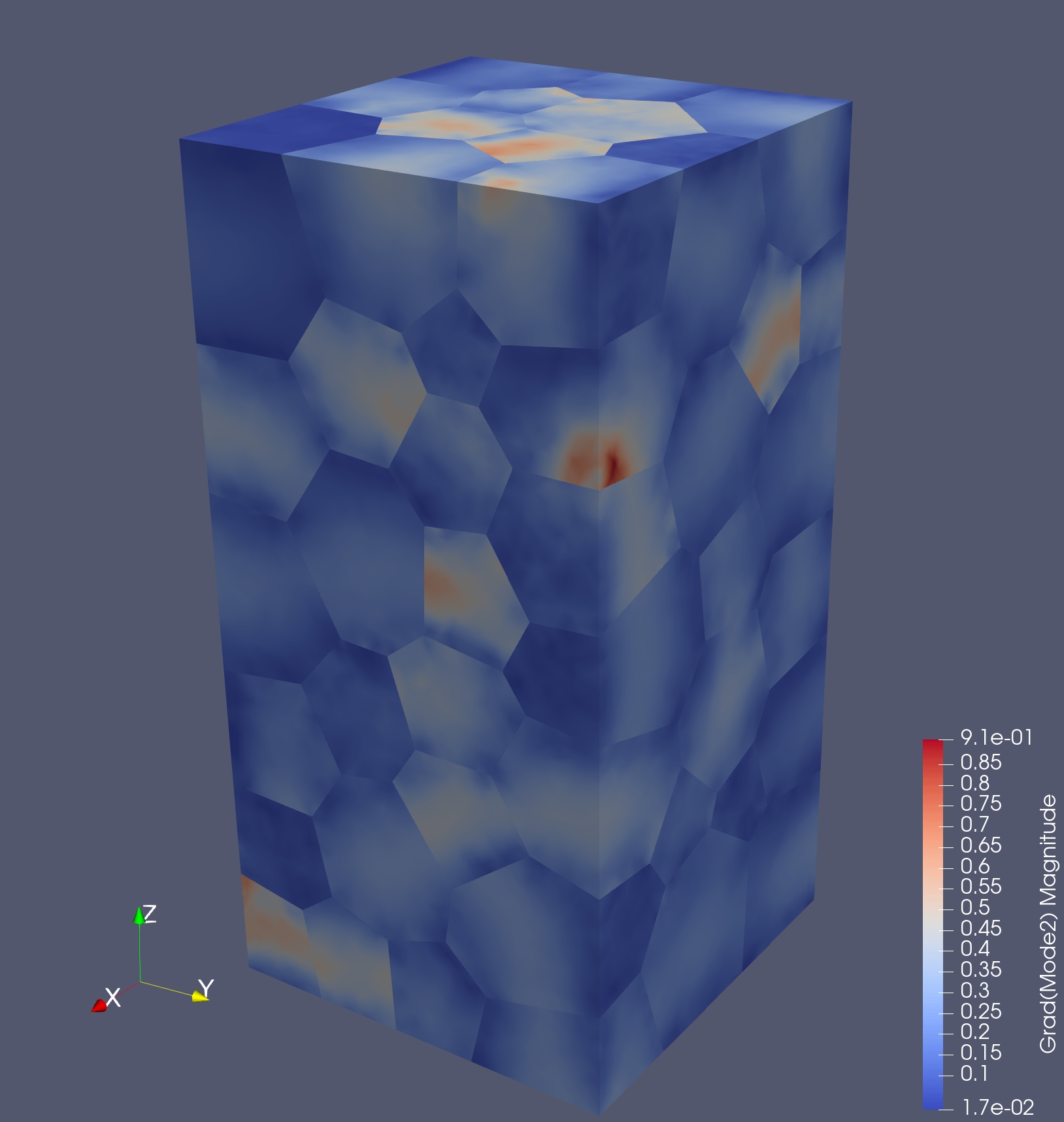
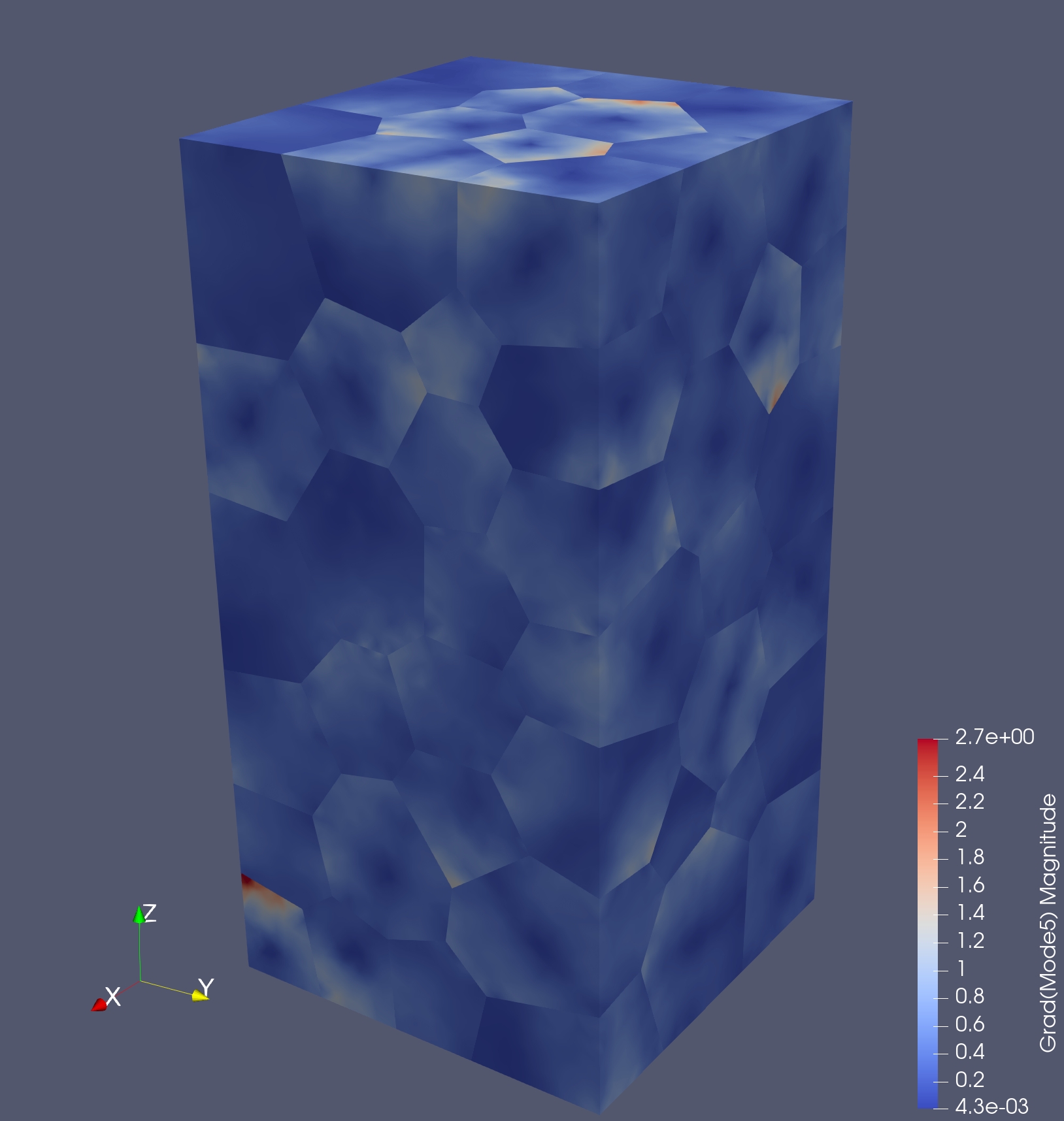
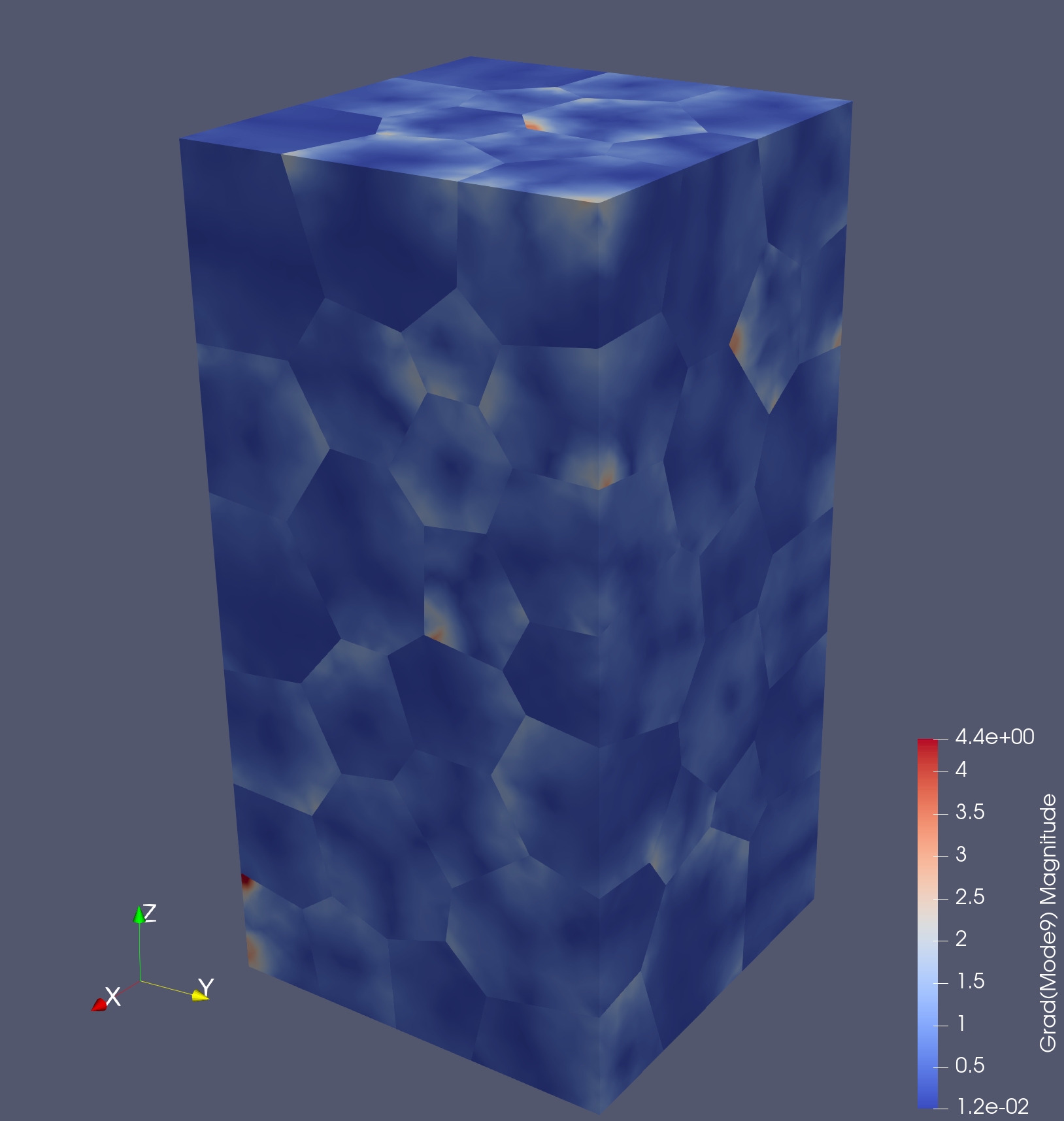
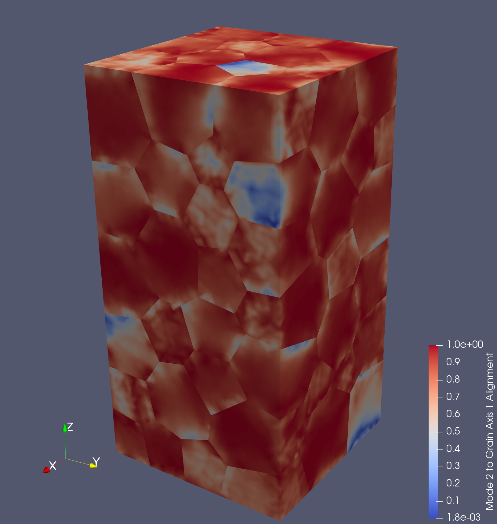
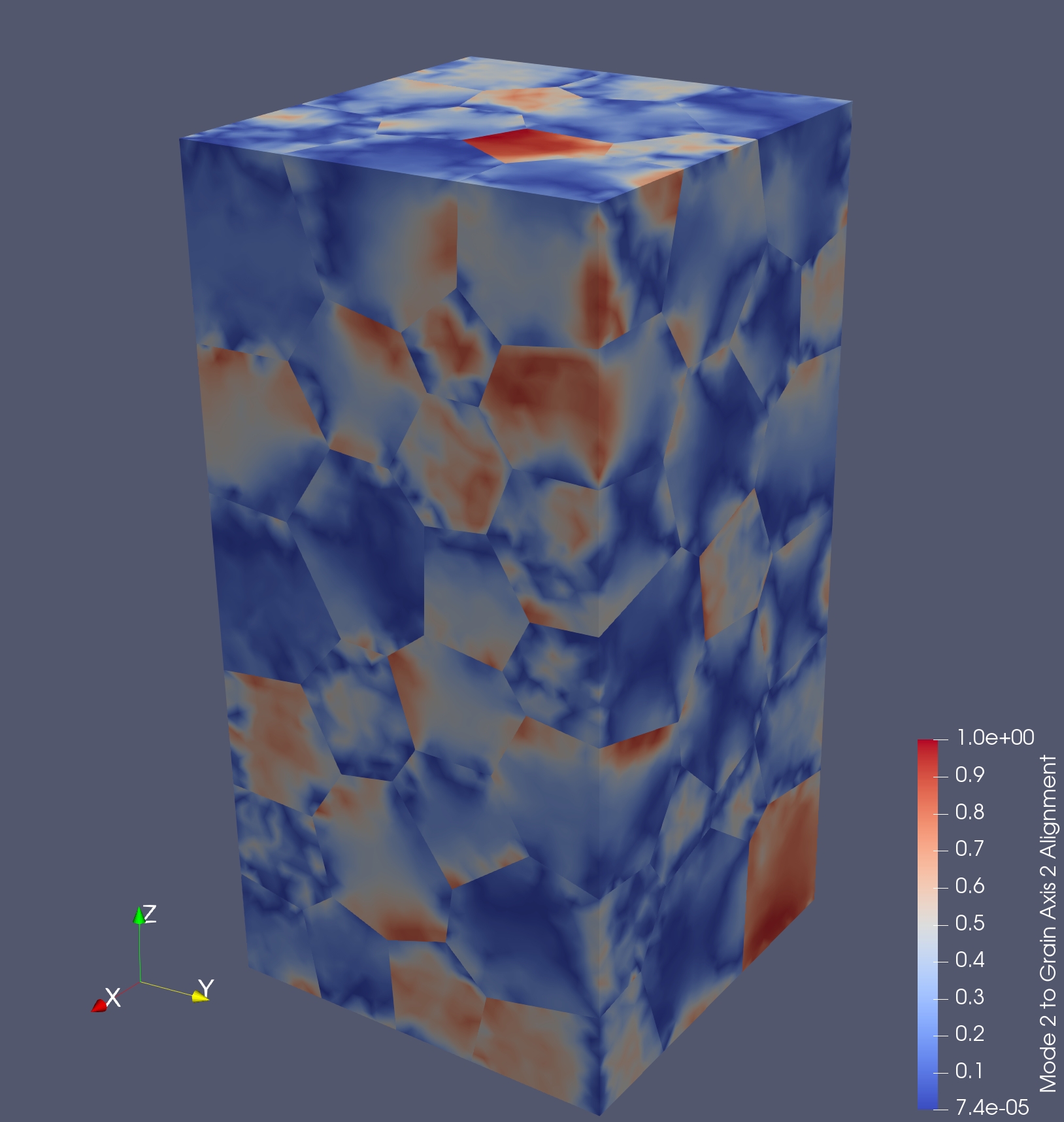
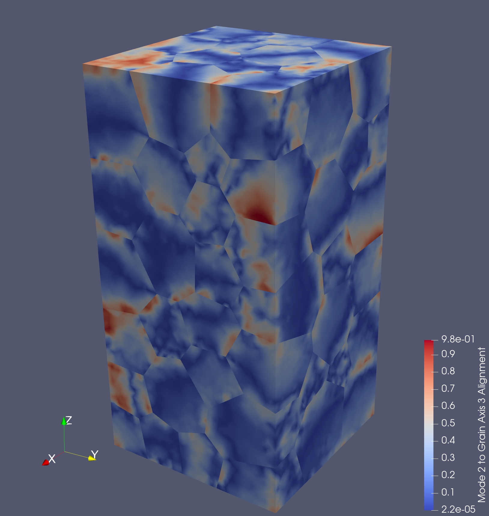
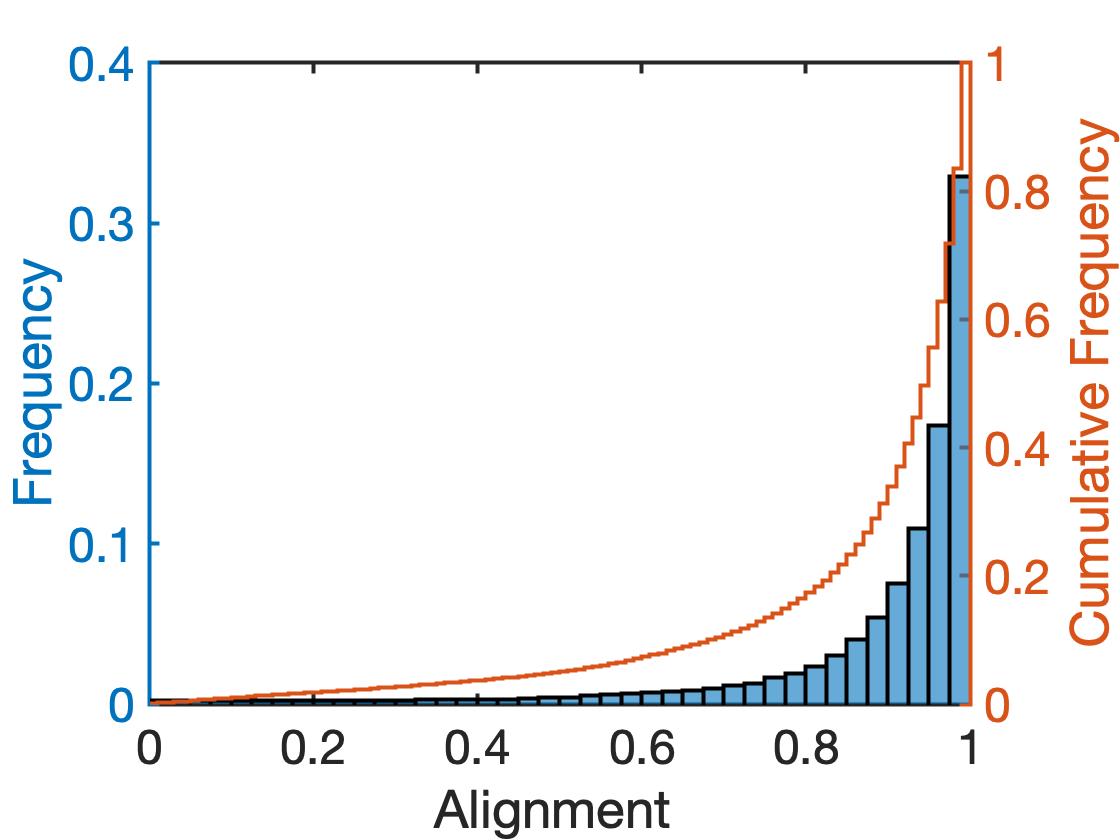
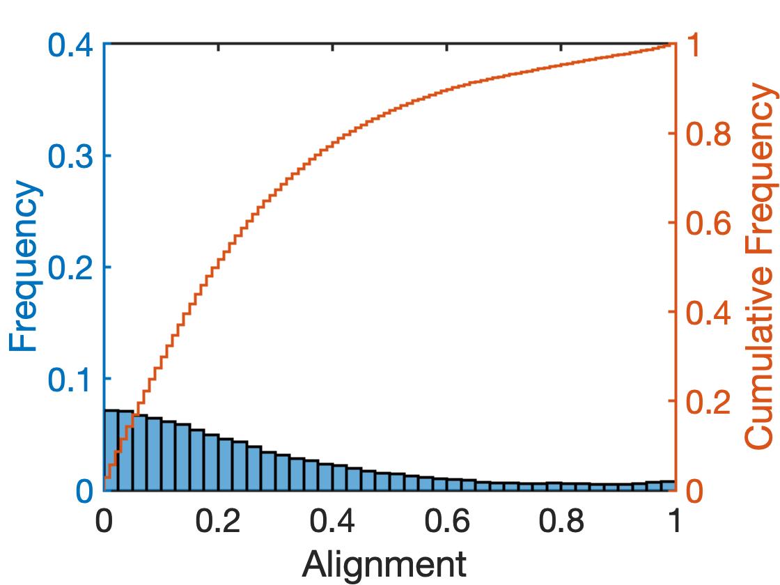
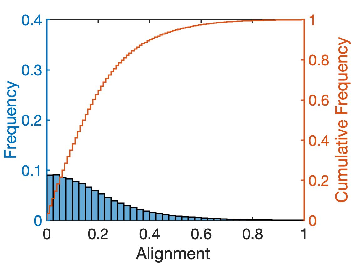
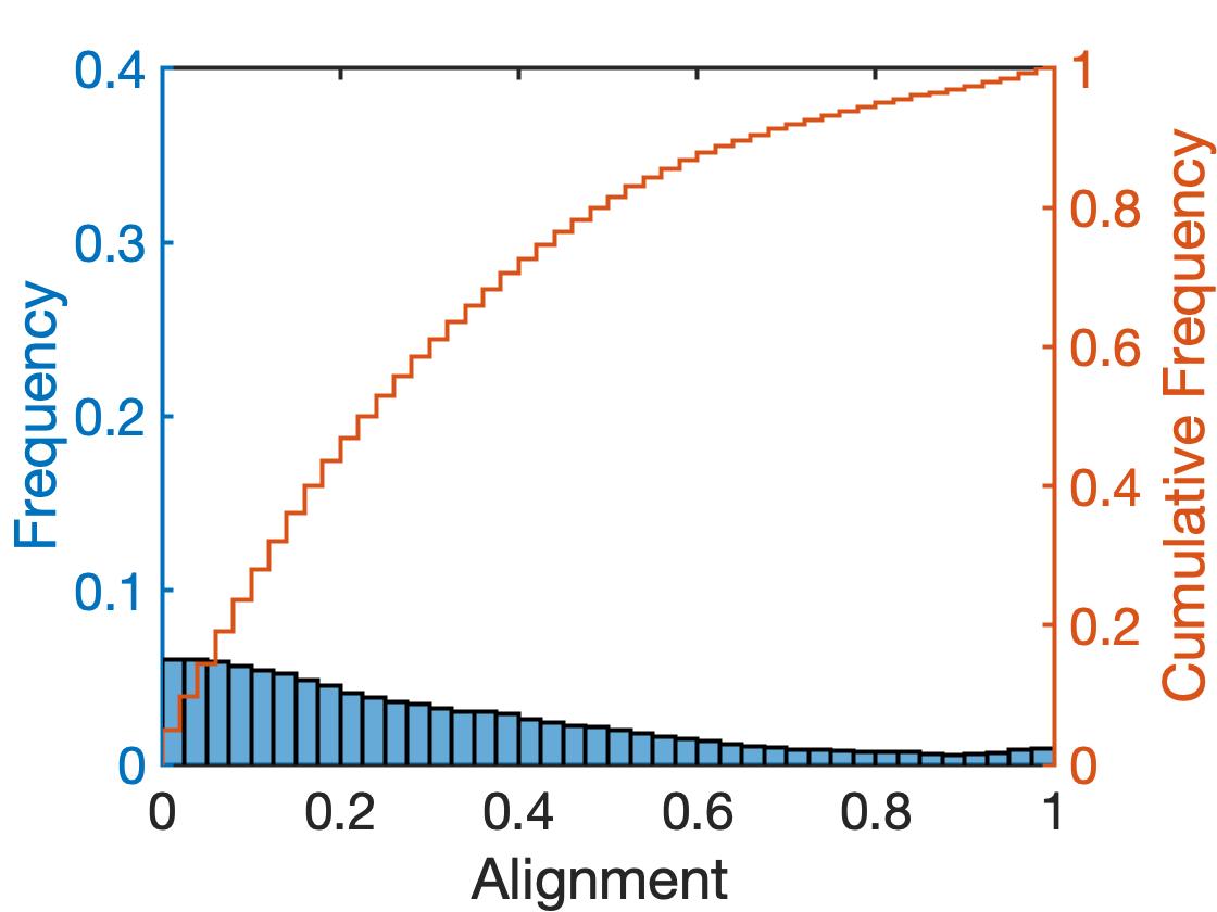
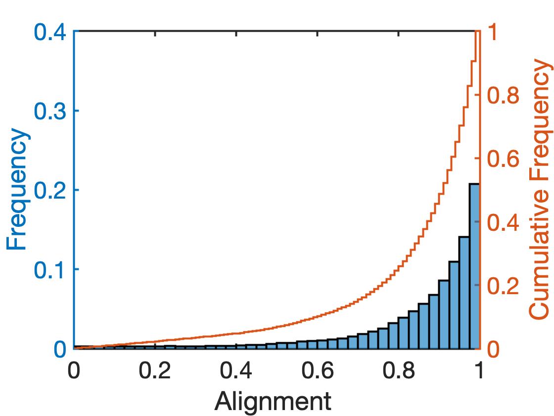
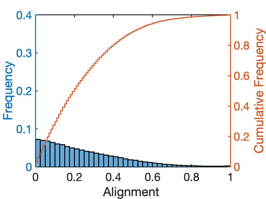
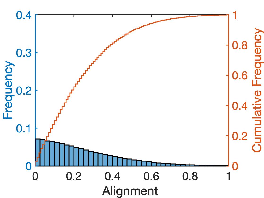
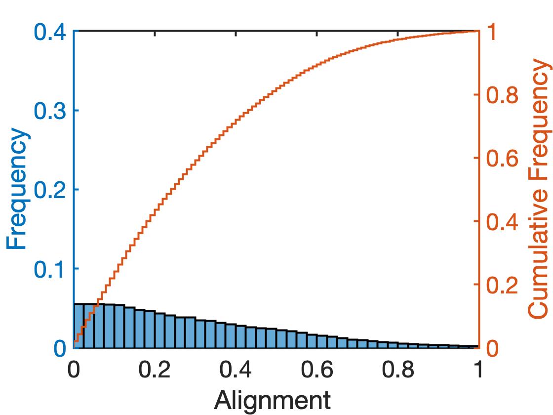
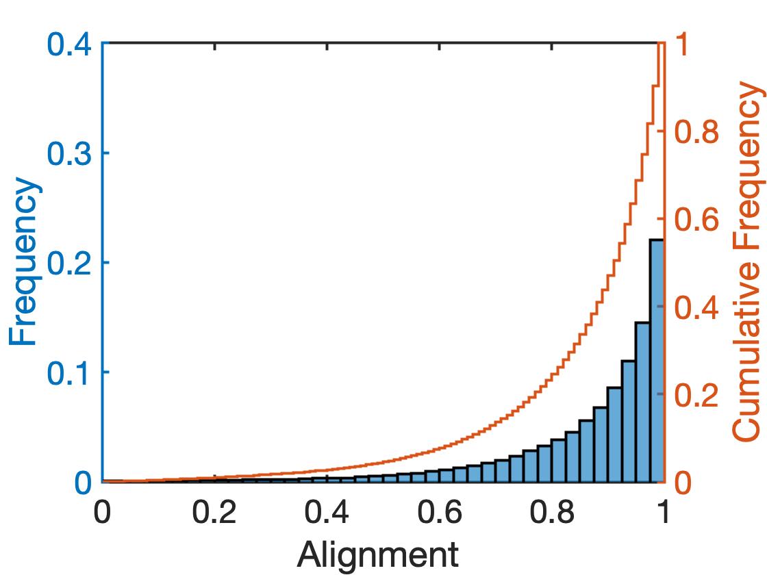
Figures 13, 14 and 15 show the gradients for Modes 2, 5 and 9 for each of the sample variants. Here we show the magnitudes of the vector gradients. Although the direction of the modes (the gradient vector) appear to be haphazard, there is a correlation with the grain axes. Figure 16 displays the alignment of the gradient vector for Mode 2 with each of the three grain axis vectors obtained from the dot product of the two vectors for the HUHS sample variant. Visually this plot suggest a strong correlation. Figures 17, 18 and 19 show the frequency distributions for the first three modes of the HUHS sample variant with respect to the three grain axes. What can be inferred from the visual display in Figure 16 is confirmed statistically in these plots for the first three (non-constant) modes: the gradient vector of Mode 2 aligns with the major diameter axis while the gradient vectors of Modes 3 and 4 align with the two minor axes. Qualitatively similar distributions exist for the Voronoi and LULS sample variants. We have not explored the correlations between higher modes and the grain axes, but suspect correlations do exist.

(a)

(b)

(c)

Figure 13: Harmonic mode gradients of the Voronoi sample. (a) Mode 2; (b) Mode 5; (c) Mode 9.

(a)

(b)

(c)

Figure 14: Harmonic mode gradients of the LULS sample. (a) Mode 2; (b) Mode 5; (c) Mode 9.

(a)

(b)

(c)

Figure 15: Harmonic modes gradient of the HUHS sample. (a) Mode 2; (b) Mode 5; (c) Mode 9.

(a)

(b)

(c)

Figure 16: Alignment of the gradient vector in the HUHS sample for Mode 2 with the grain axes: (a) grain axis 1; (b) grain axis 2; (c) grain axis 3.

(a)

(b)

(c)

Figure 17: Frequency distribution for the alignment of the gradient vector in the HUHS sample for Mode 2 with the grain axes: (a) grain axis 1; (b) grain axis 2; (c) grain axis 3.

(a)

(b)

(c)

Figure 18: Frequency distribution for the alignment of the gradient vector in the HUHS sample for Mode 2 with the grain axes: (a) grain axis 1; (b) grain axis 2; (c) grain axis 3.

(a)

(b)

(c)

Figure 19: Frequency distribution for the alignment of the gradient vector in the HUHS sample for Mode 3 with the grain axes: (a) grain axis 1; (b) grain axis 2; (c) grain axis 3.

3.4 Simulated responses of samples using FEpX

Data for this demonstration application were generated with the finite element code, FEpX. FEpX  simulates the elasto-viscoplastic response of polycrystals over loading sequences that can induce large strain deformations. The constitutive behaviors are defined at the crystal scale: anisotropic elasticity given by Hooke’s law and anisotropic plasticity resulting from slip on a limited number of slip systems (referred to as restricted slip). Slip is rate dependent. The nonlinear solution algorithms facilitate the specification of low rate sensitivity as is typically the case of metallic alloys at low homologous temperatures. For the simulation of the three sample variants, the single crystal properties of a FCC stainless steel (AL6XN) were chosen. The determination of the needed parameters is documented in [7].

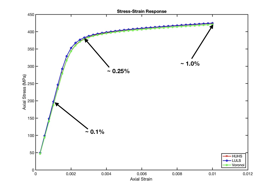
The samples variants all were subjected to the same loading: extension in the $z$ coordinate at fixed ’cross-head’ velocity to a nominal strain of 1%. 40 equal time steps were used to reach the nominal strain. The lateral surfaces of the sample variants were traction-free. The tractions on the exterior surfaces were integrated over those surfaces to generate nominal stress-strain curves, as shown in Figure 20. Small variations in the stress can be observed, particularly through the elastic-plastic transition (the knee of the curve).

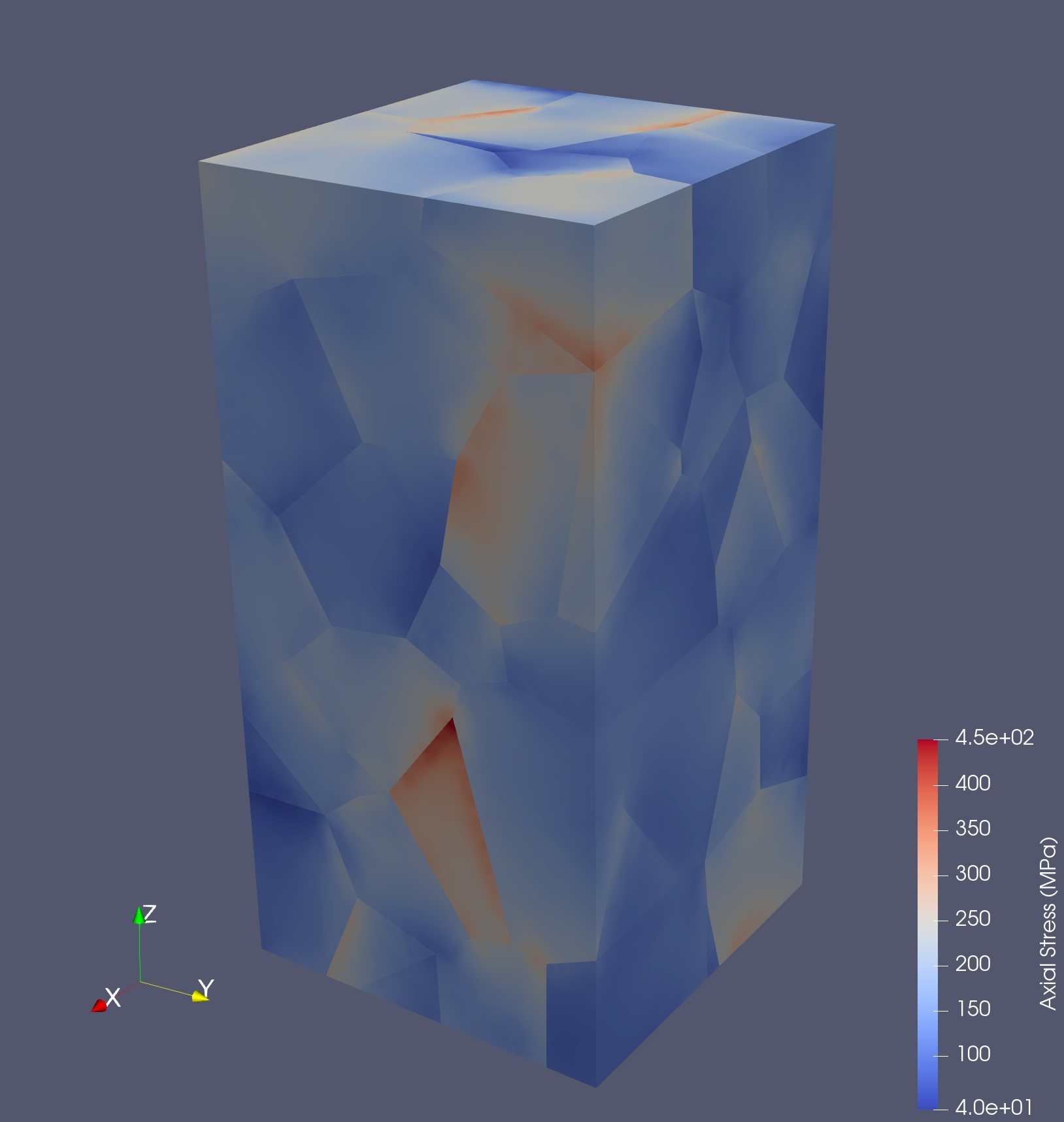
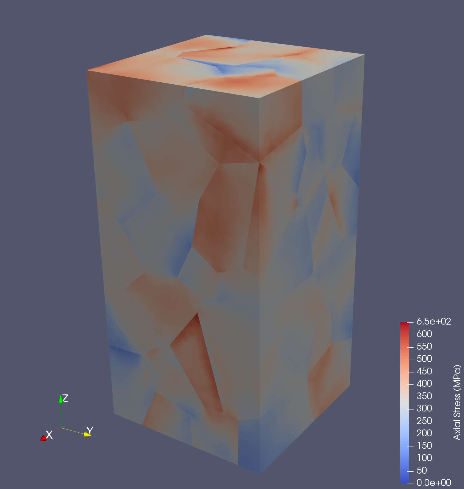
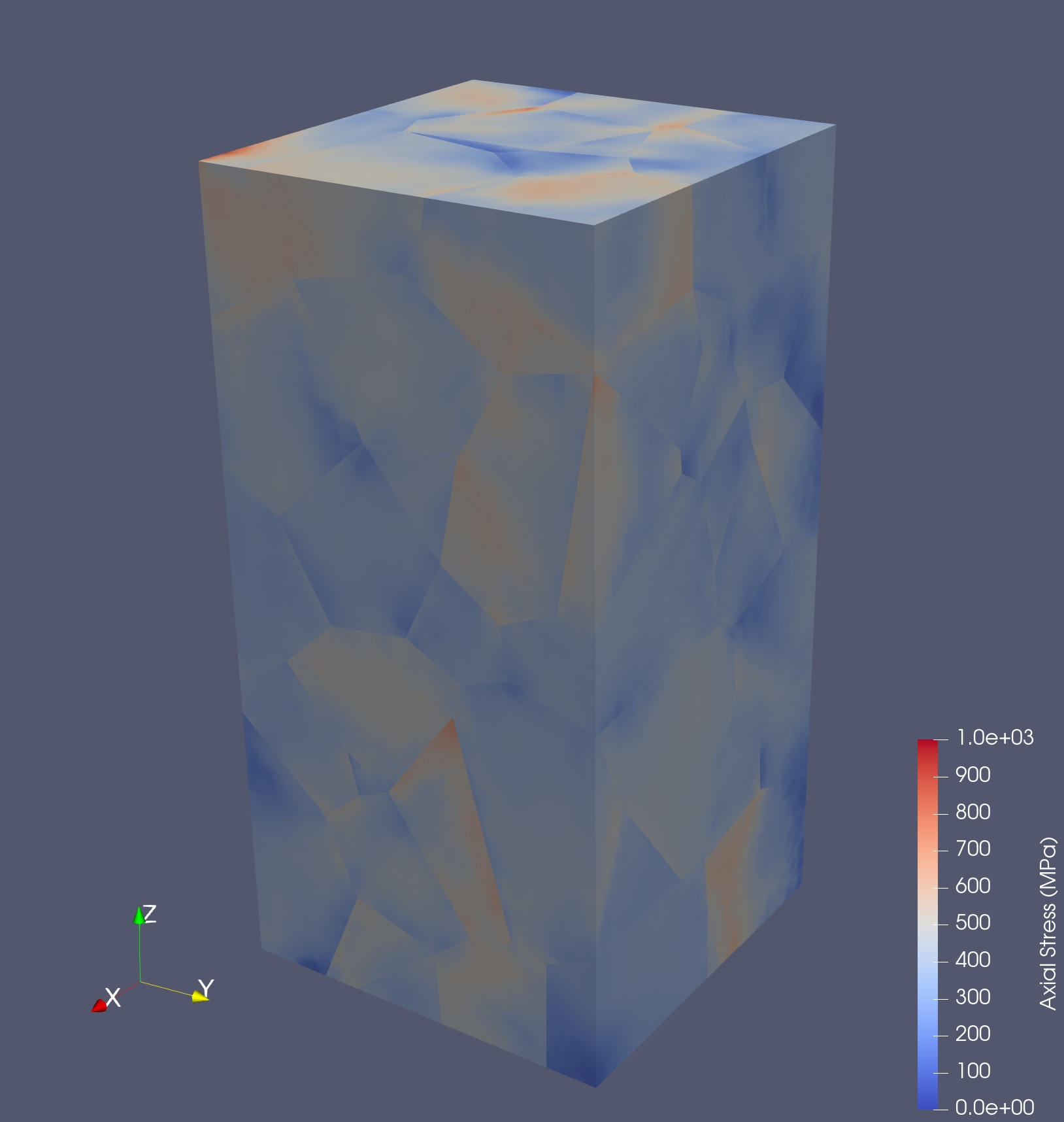
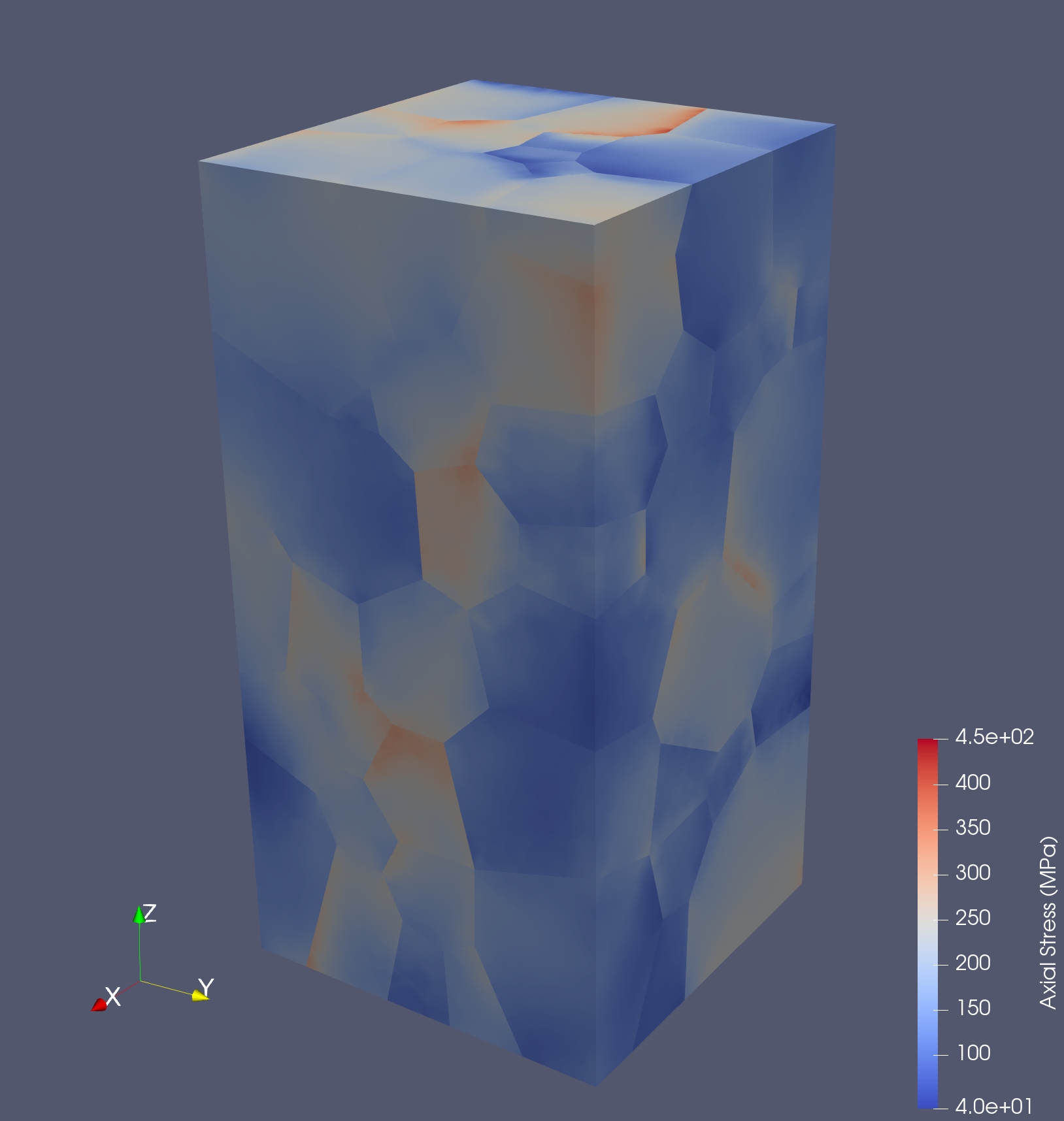
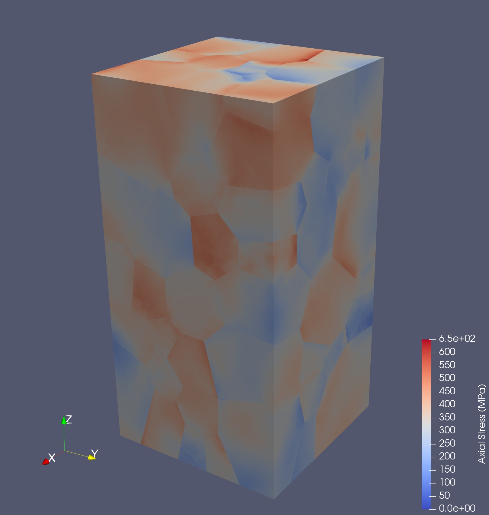
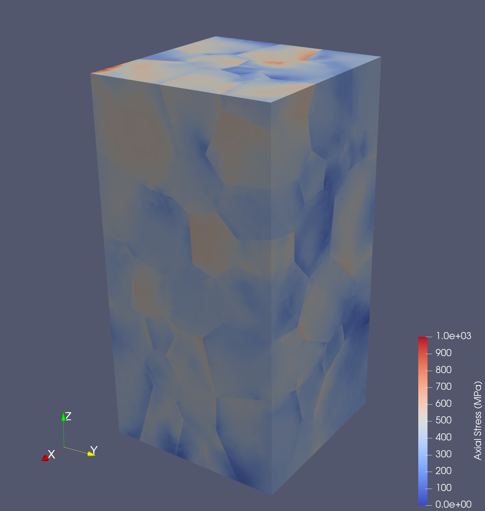
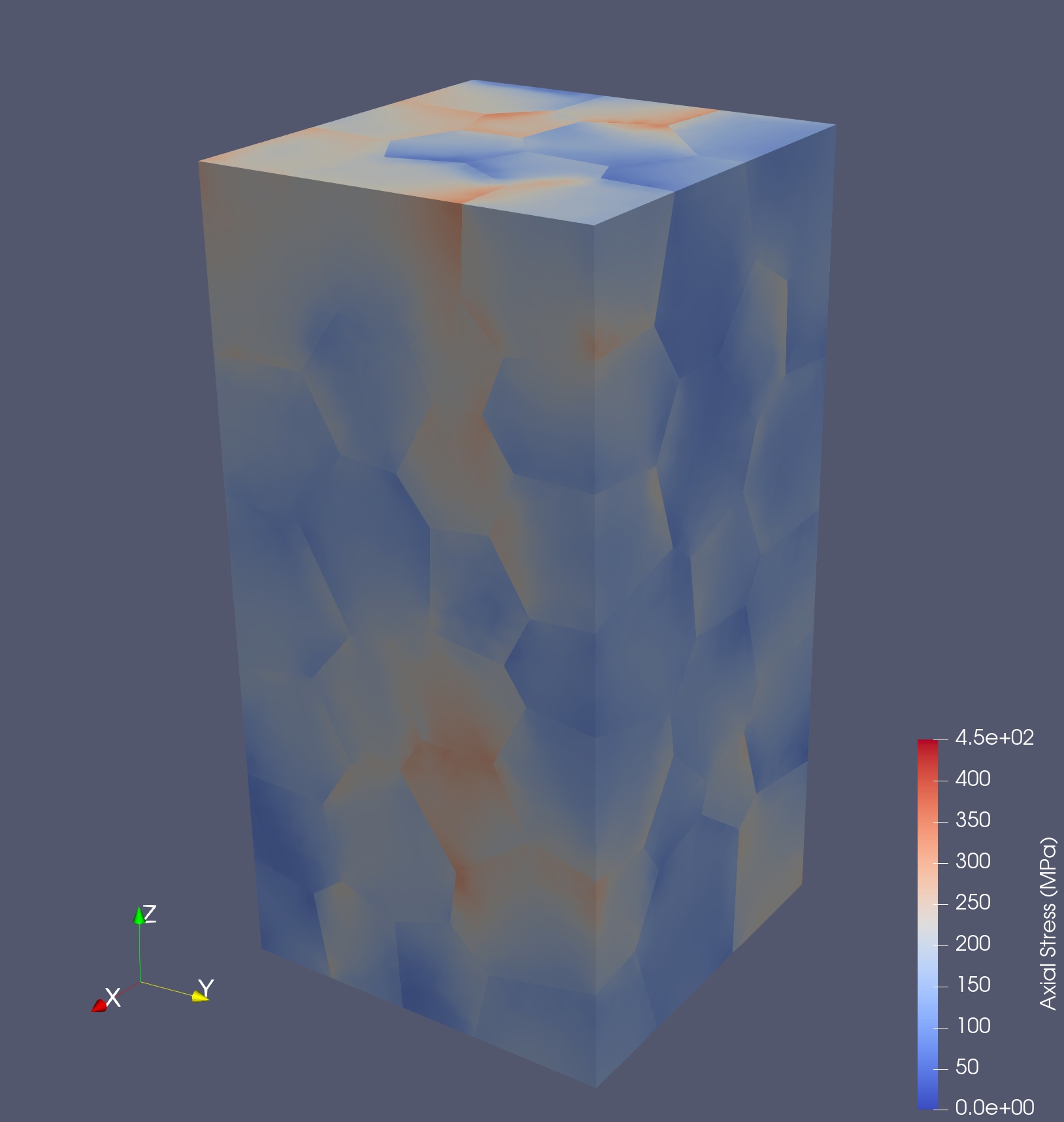
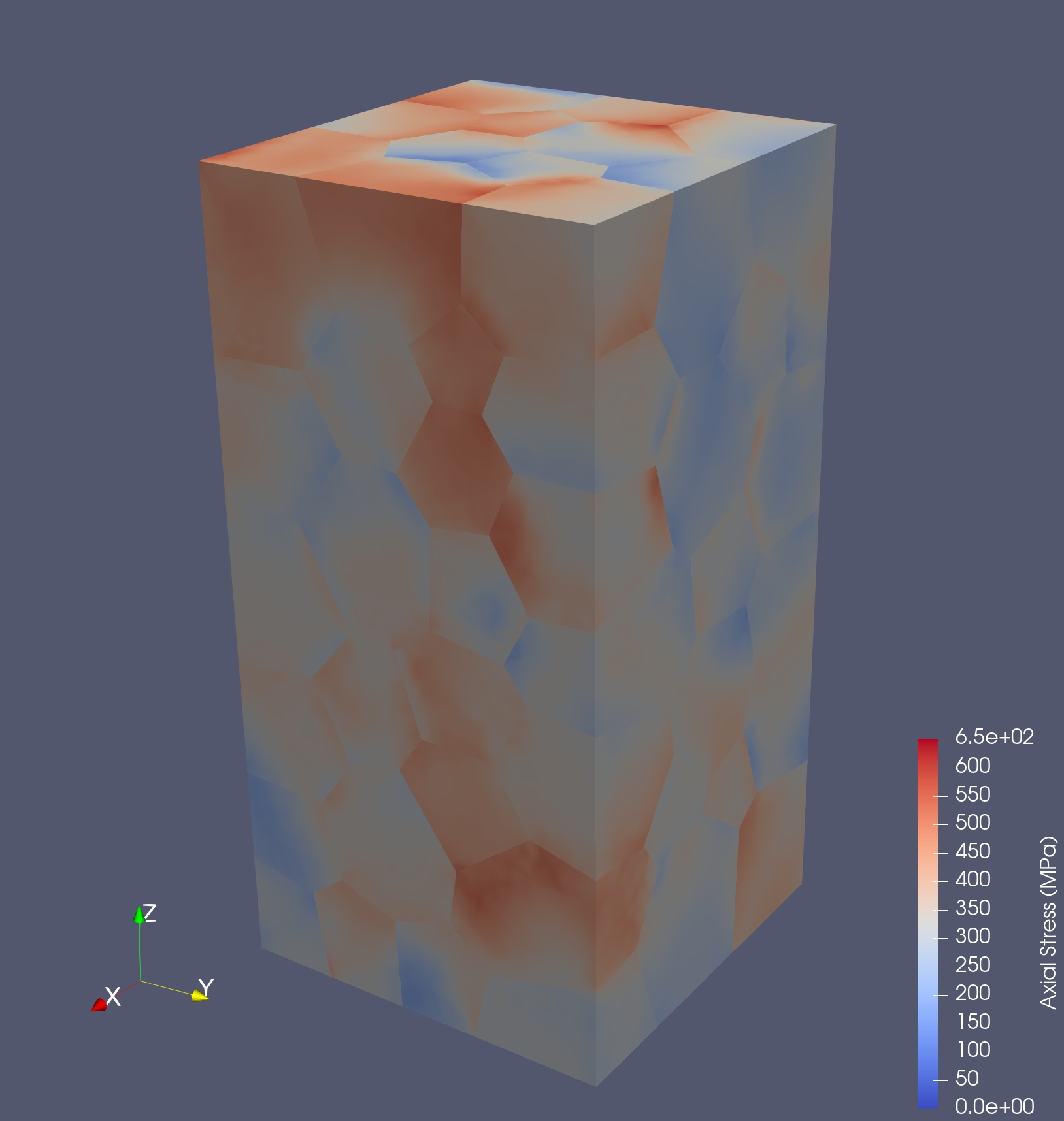
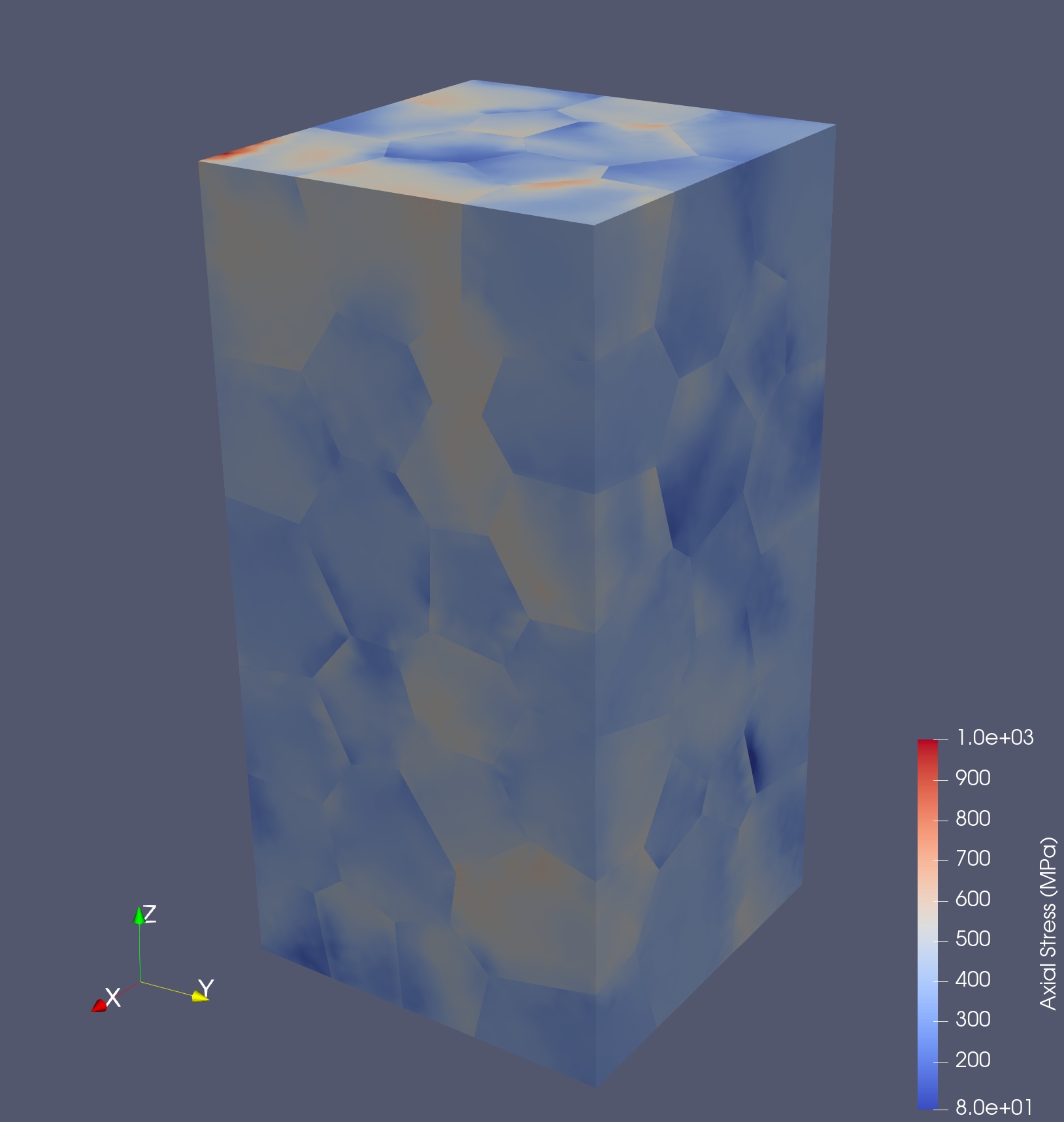
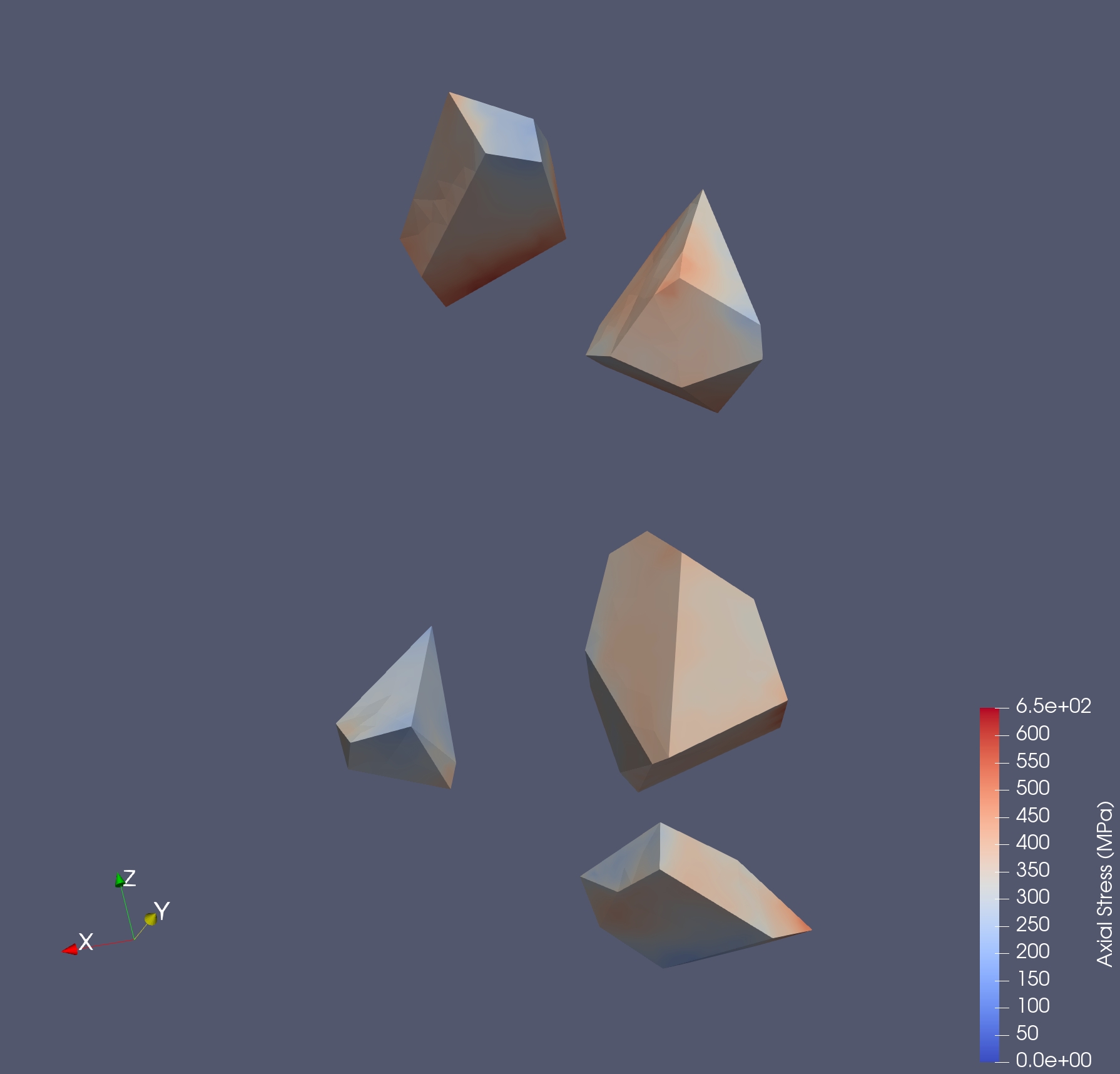
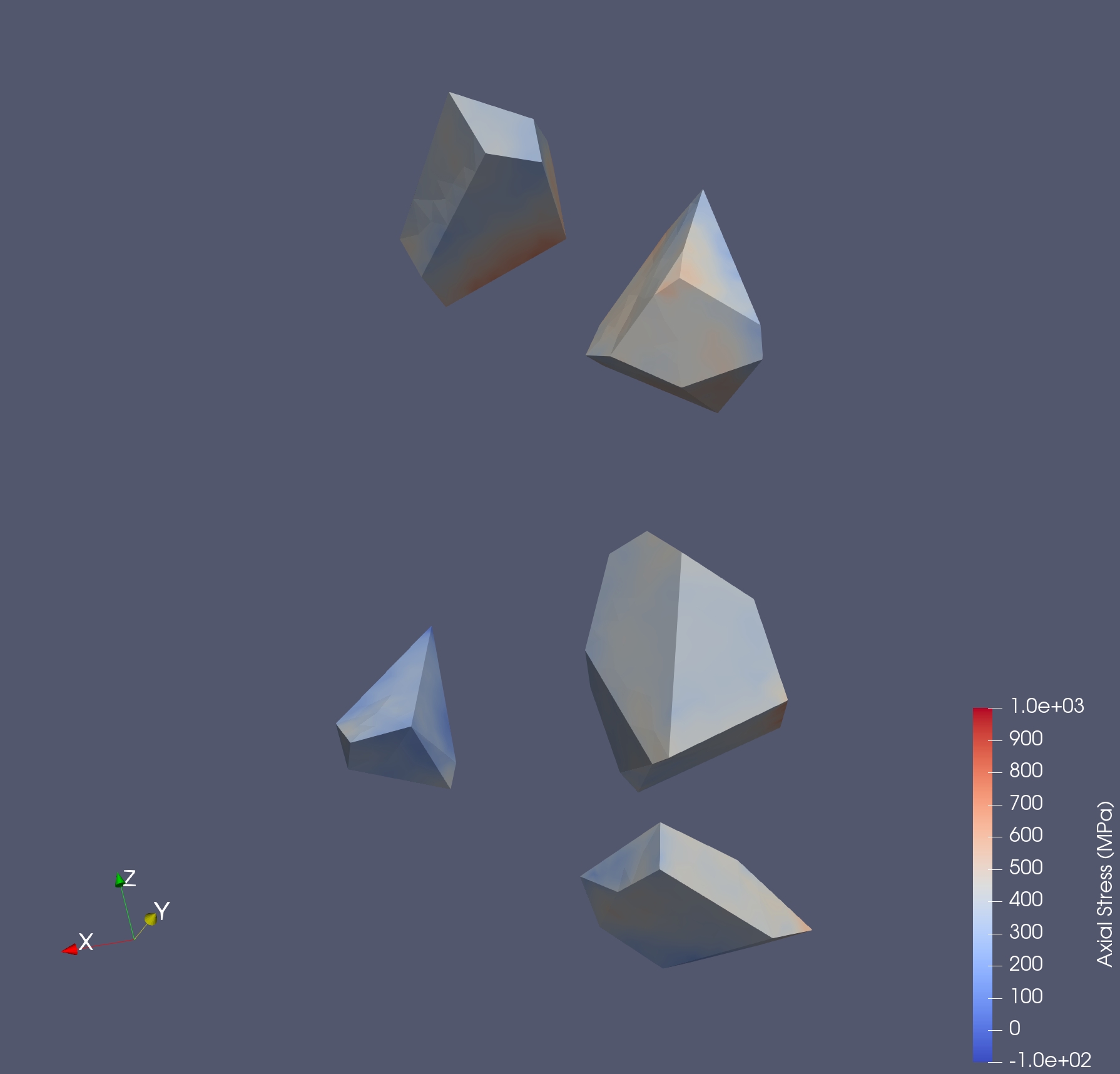
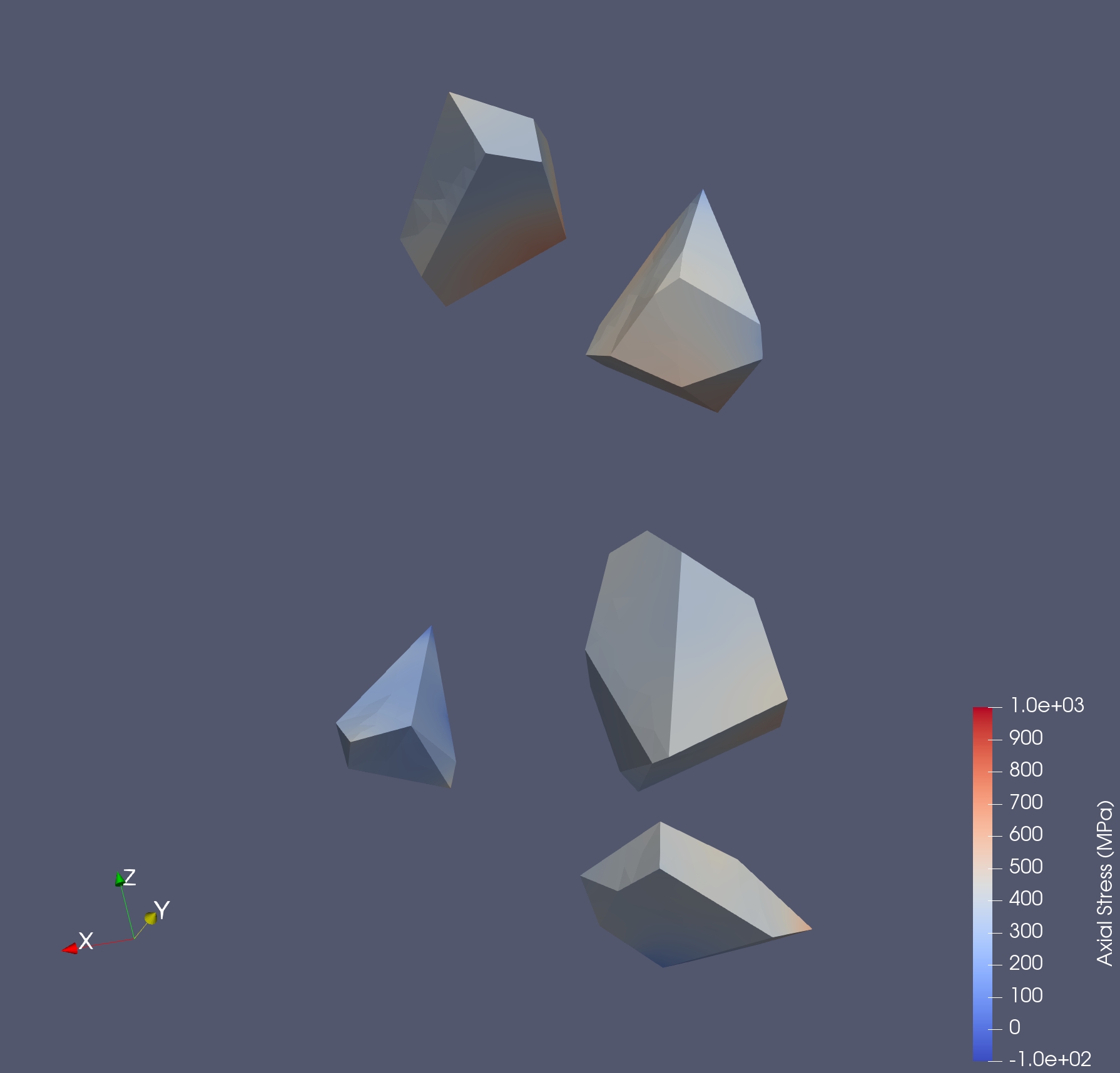
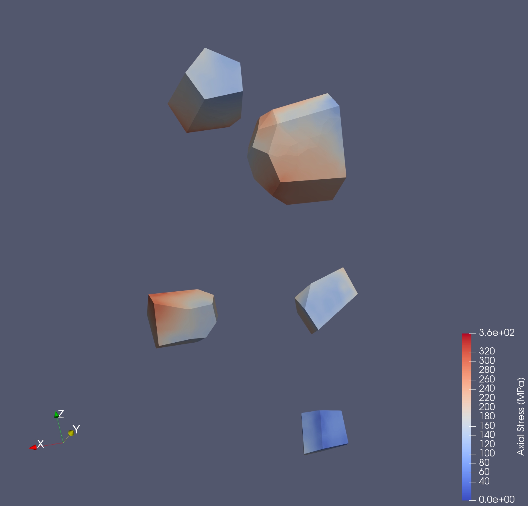
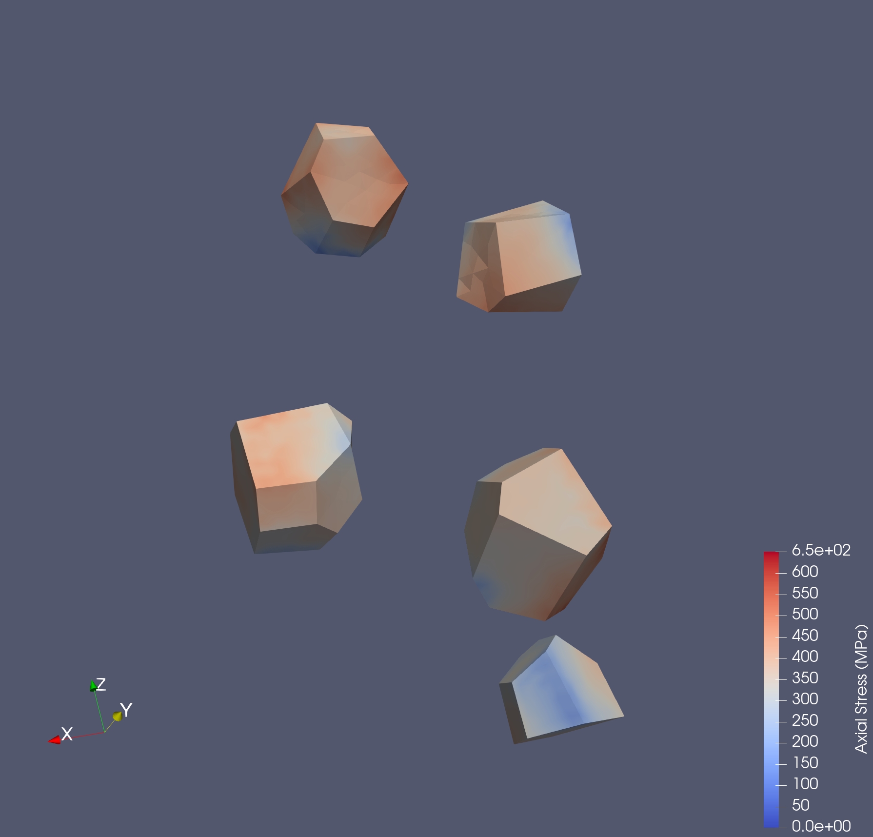
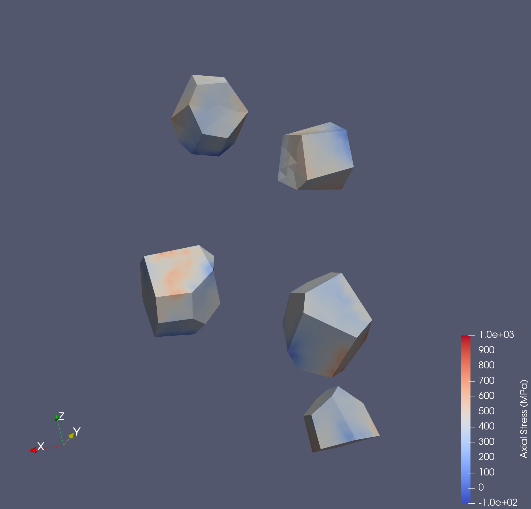
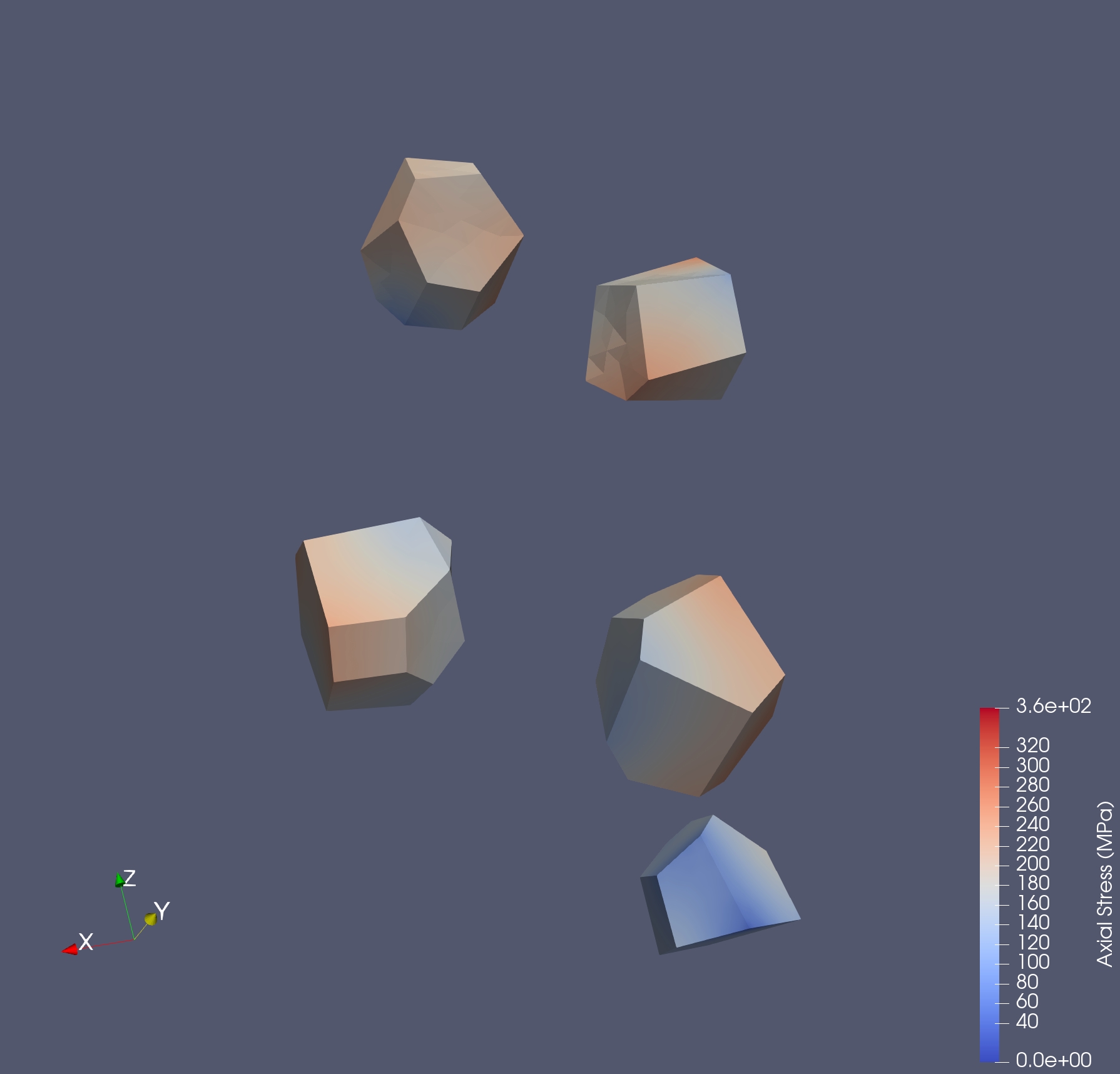
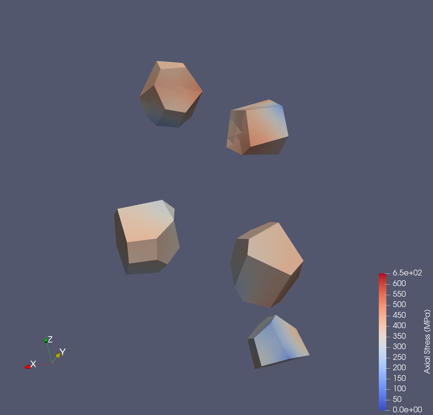
Stress distributions on full sample at three levels of nominal strain (0.1%, 0.25% and 1%) are shown in Figures 21, 22 and 23. The scales are different for the three strain levels but the same across the sample variants. Note that the first strain level, 0.1%, is the same as that specified for the elastic MechMet  analyses presented in Section 3.2. Similarities of the stress distributions do appear to exist across the sample variants. However, the most noteworthy feature is the changes in the patterns of stress that occur as loading proceeds through the elastic-plastic transition, indicating that the stress re-distributes with the onset of yielding.

Figure 20: Stress-strain curves for the Voronoi, LULS and HUHS samples for axial extension to 1% nominal strain in the $z$ direction.

(a)

(b)

(c)

Figure 21: Axial stress distributions over the Voronoi sample using FEpX  at nominal axial strains of (a) 0.1% ; (b) 0.25%; and (c) 1.0%. Note that each distribution has its own scale.

(a)

(b)

(c)

Figure 22: Axial stress distributions over the LULS sample using FEpX  at nominal axial strains of (a) 0.1% ; (b) 0.25%; and (c) 1.0%. Note that each distribution has its own scale.

(a)

(b)

(c)

Figure 23: Axial stress distributions over the HUHS sample using FEpX  at nominal axial strains of (a) 0.1% ; (b) 0.25%; and (c) 1.0%. Note that each distribution has its own scale.

3.5 Harmonic representation of stress in 5 grains

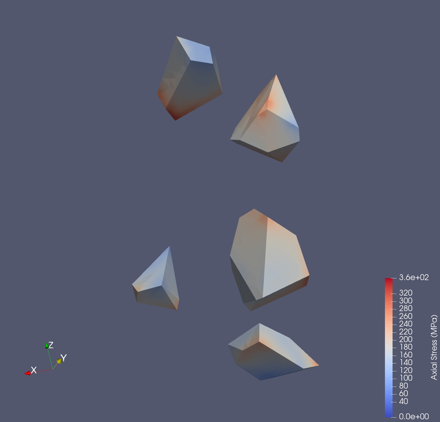
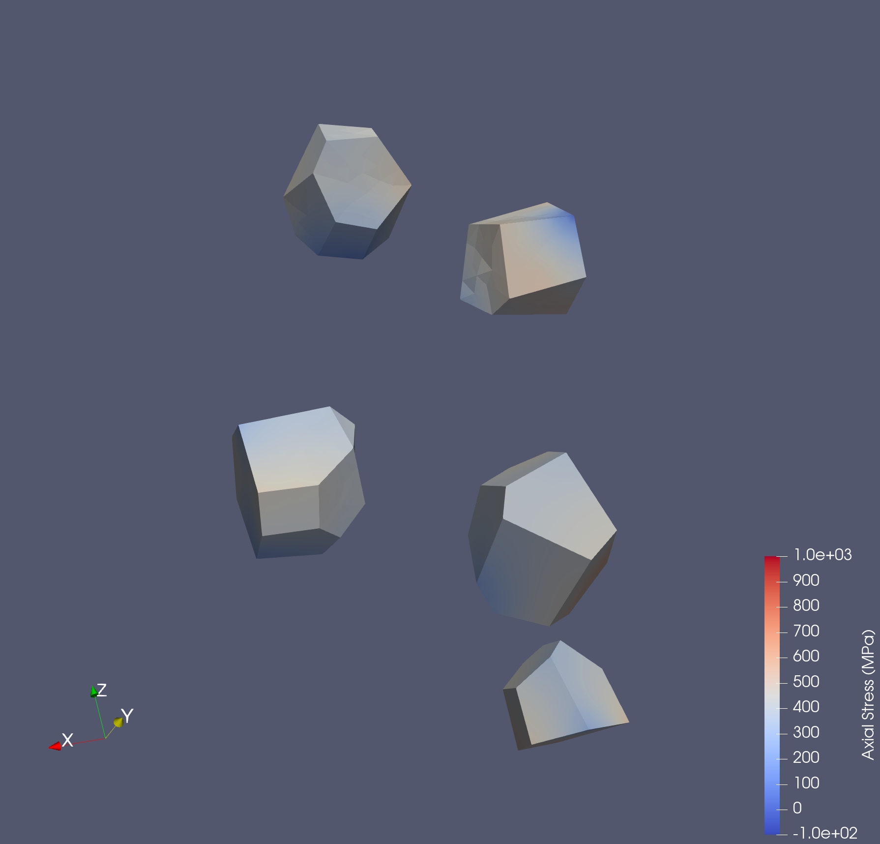
We have chosen 5 grains to examine individually: Grains 48, 49, 50, 51, and 52. These are the 5 grains in the middle of the numbered list and were chosen simply for convenience and because they were not end grains (having a facet on the loaded surface). The same five grains are examined for all three sample variants. Figure 24 shows the sets of grains. The morphological attributes built into the variants are evident: grains of the Voronoi sample have more irregular shapes; grains of the LULS sample have greater size variations; grains of the HUHS sample have more most regular shapes and most similar sizes.

Modes 2, 5 and 9 for the 5 grains for all three sample variants are shown in Figures 25, 26, and 27, respectively. As is the case for the entire sample, presented in Section 3.3, the higher the mode number the more complex the mode distribution. The Mode 2 distributions appear to be monotonic, whereas the other modes definitely are not. (Note that the Voronoi Mode 2 distribution in Figure 25(a) appears to be nearly constant, but actually is not; it appear so because of the extreme values of the harmonic function at one node. )

(a)

(b)

(c)

Figure 24: Grains 48, 49, 50, 51 and 52 in: (a) Voronoi sample ; (b) LULS sample; and (c) HUHS sample. Note that grains with the same number have the same initial lattice orientation.

(a)

(b)

(c)

Figure 25: Mode 2 for Grains 48, 49, 50, 51 and 52 in: (a) Voronoi sample ; (b) LULS sample; and (c) HUHS sample. Note that the plots for the Voronoi sample are biased by an extreme value in Grain 50.

(a)

(b)

(c)

Figure 26: Mode 5 for Grains 48, 49, 50, 51 and 52 in: (a) Voronoi sample ; (b) LULS sample; and (c) HUHS sample.

(a)

(b)

(c)

Figure 27: Mode 9 for Grains 48, 49, 50, 51 and 52 in: (a) Voronoi sample ; (b) LULS sample; and (c) HUHS sample.

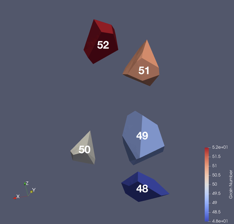
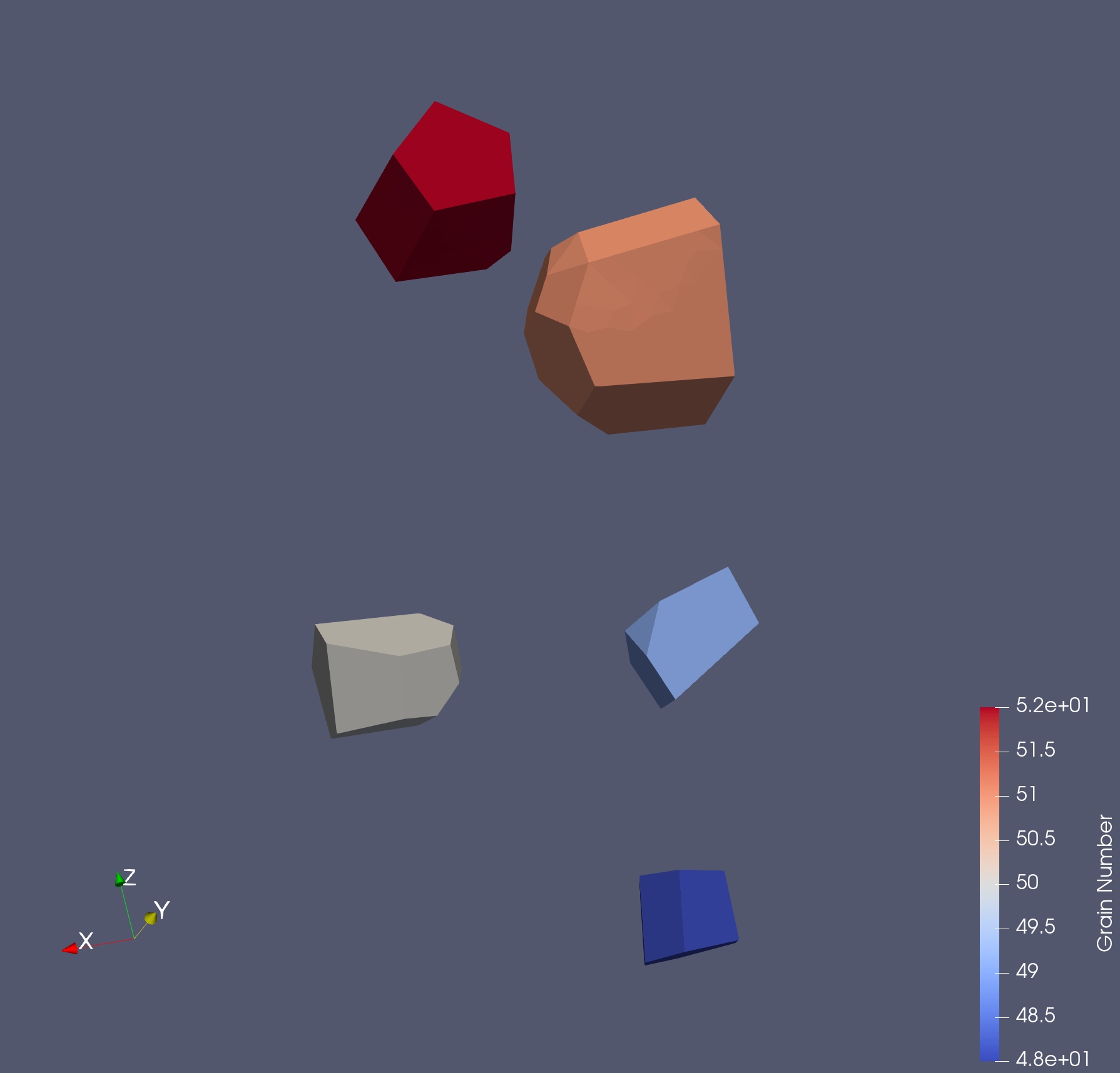
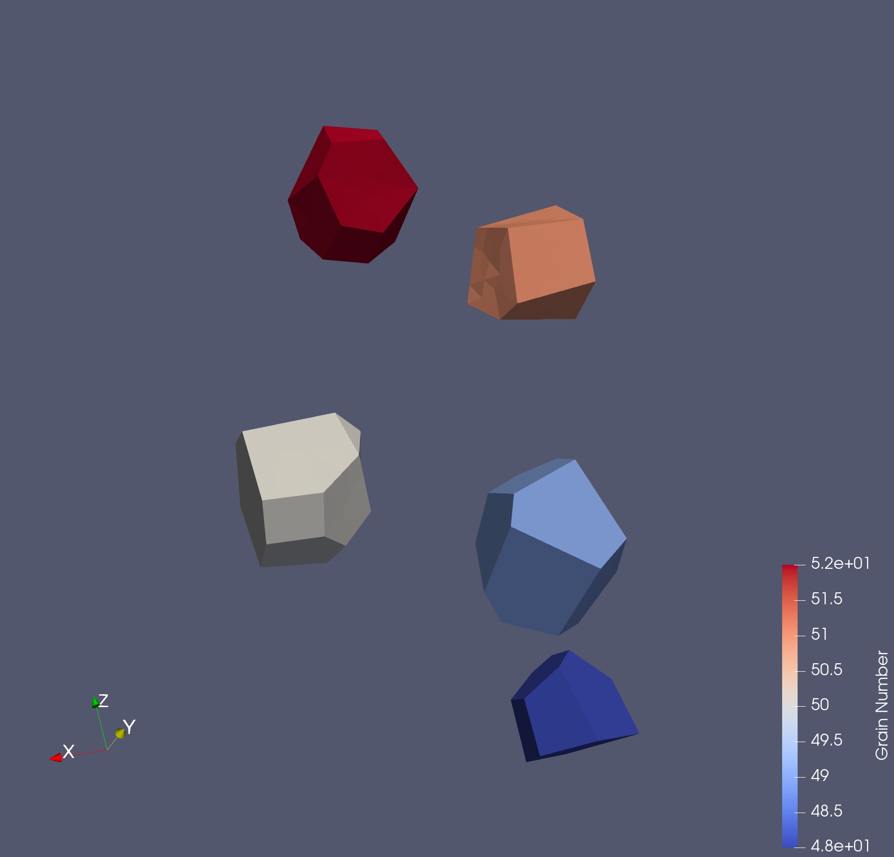
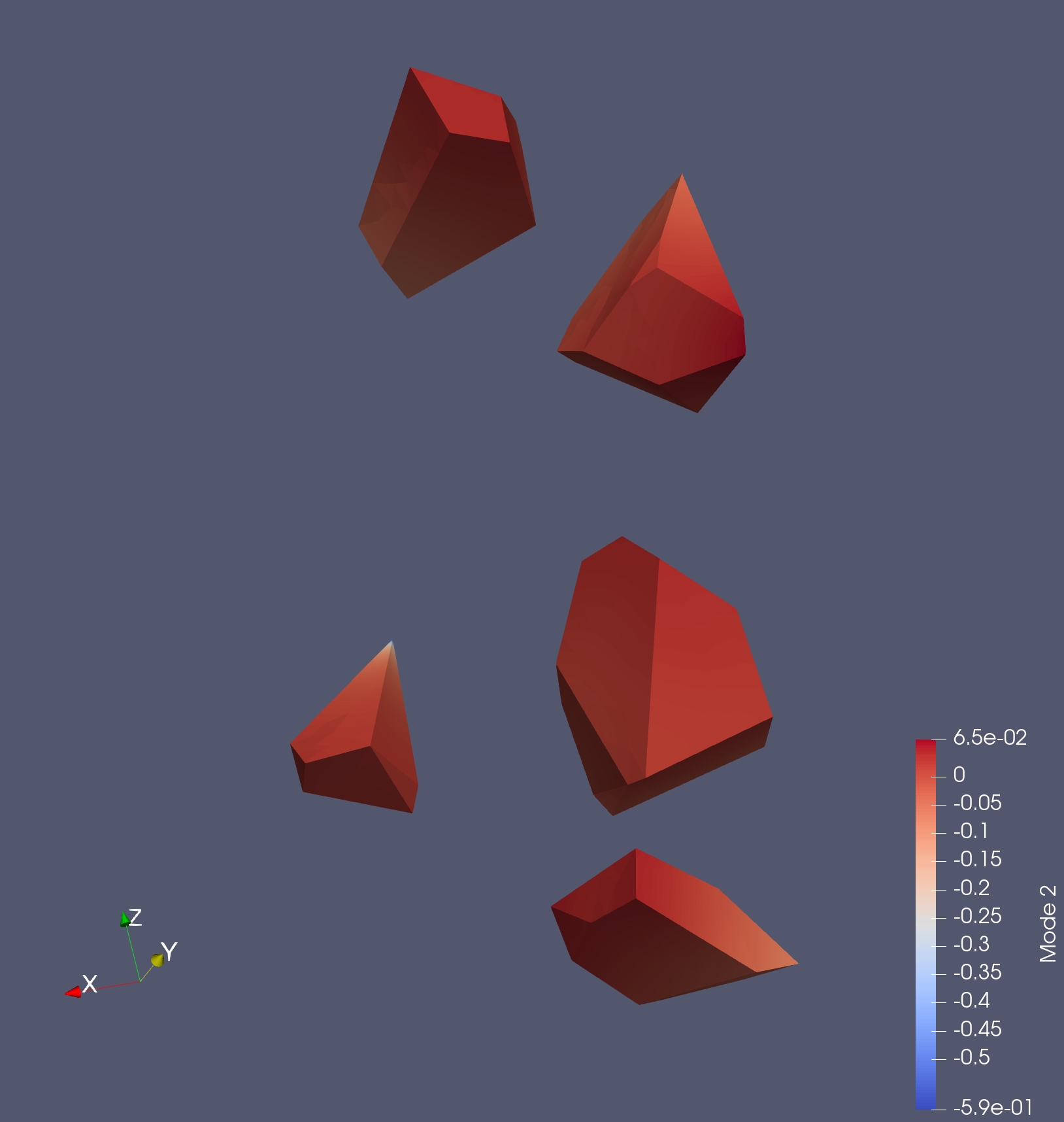
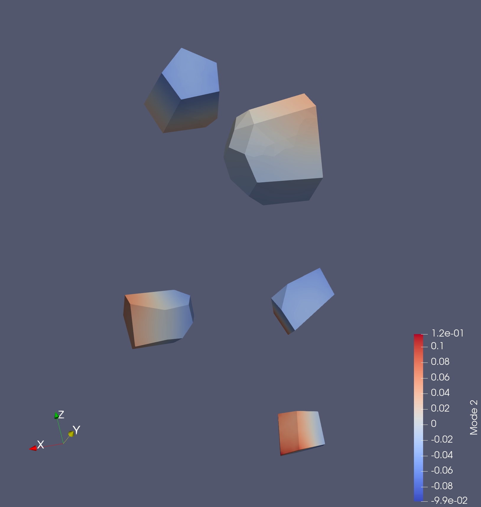
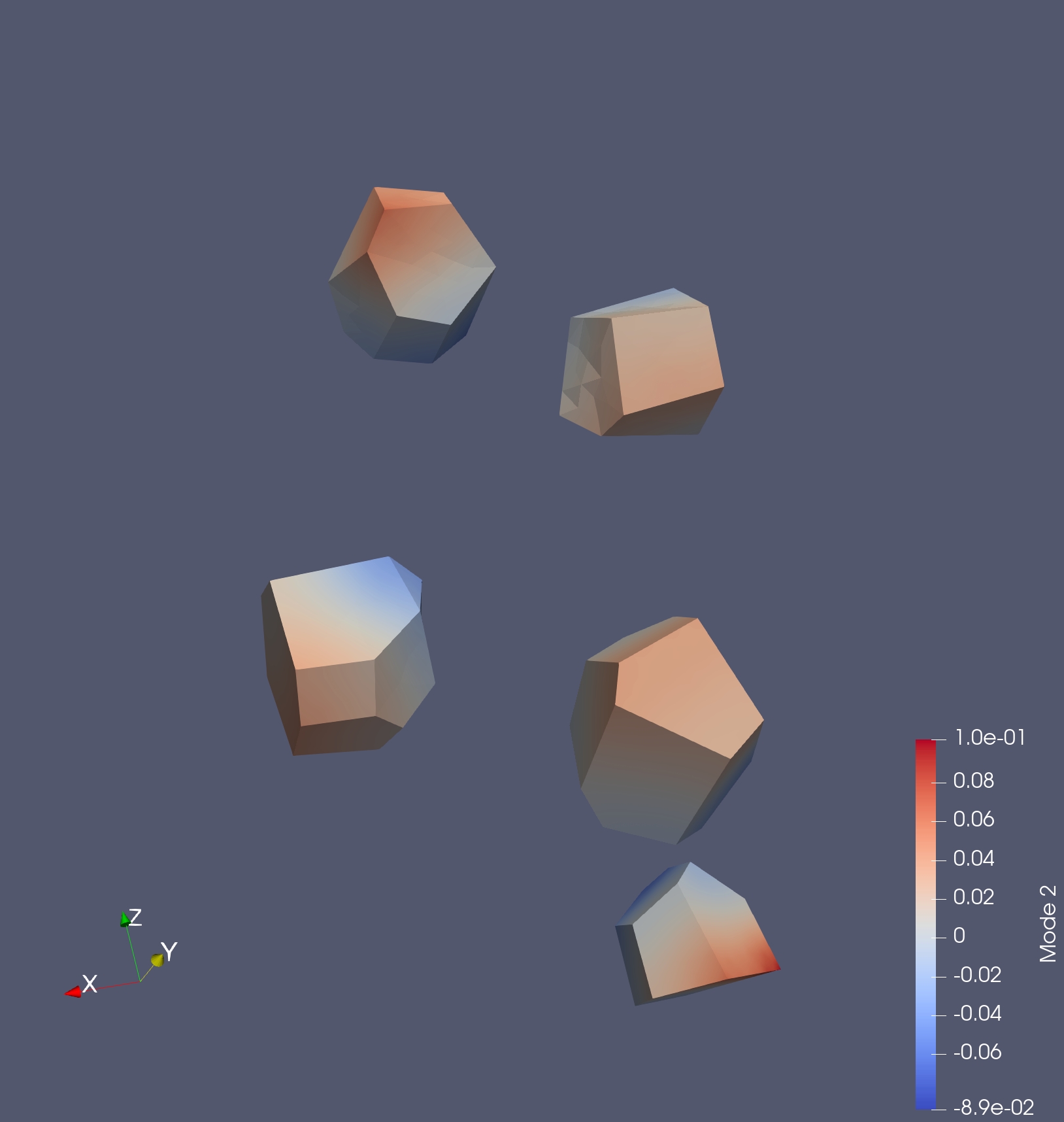
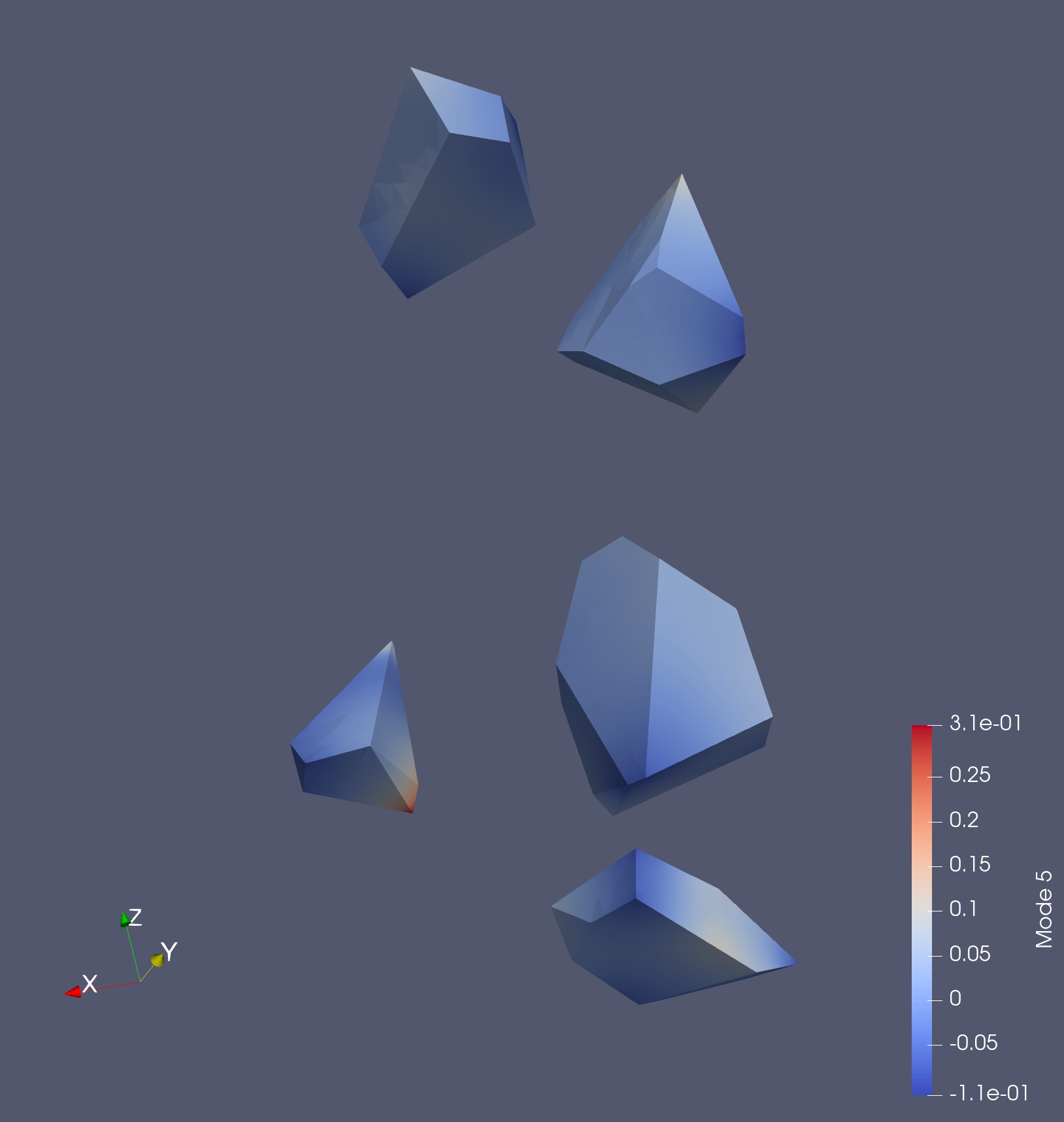
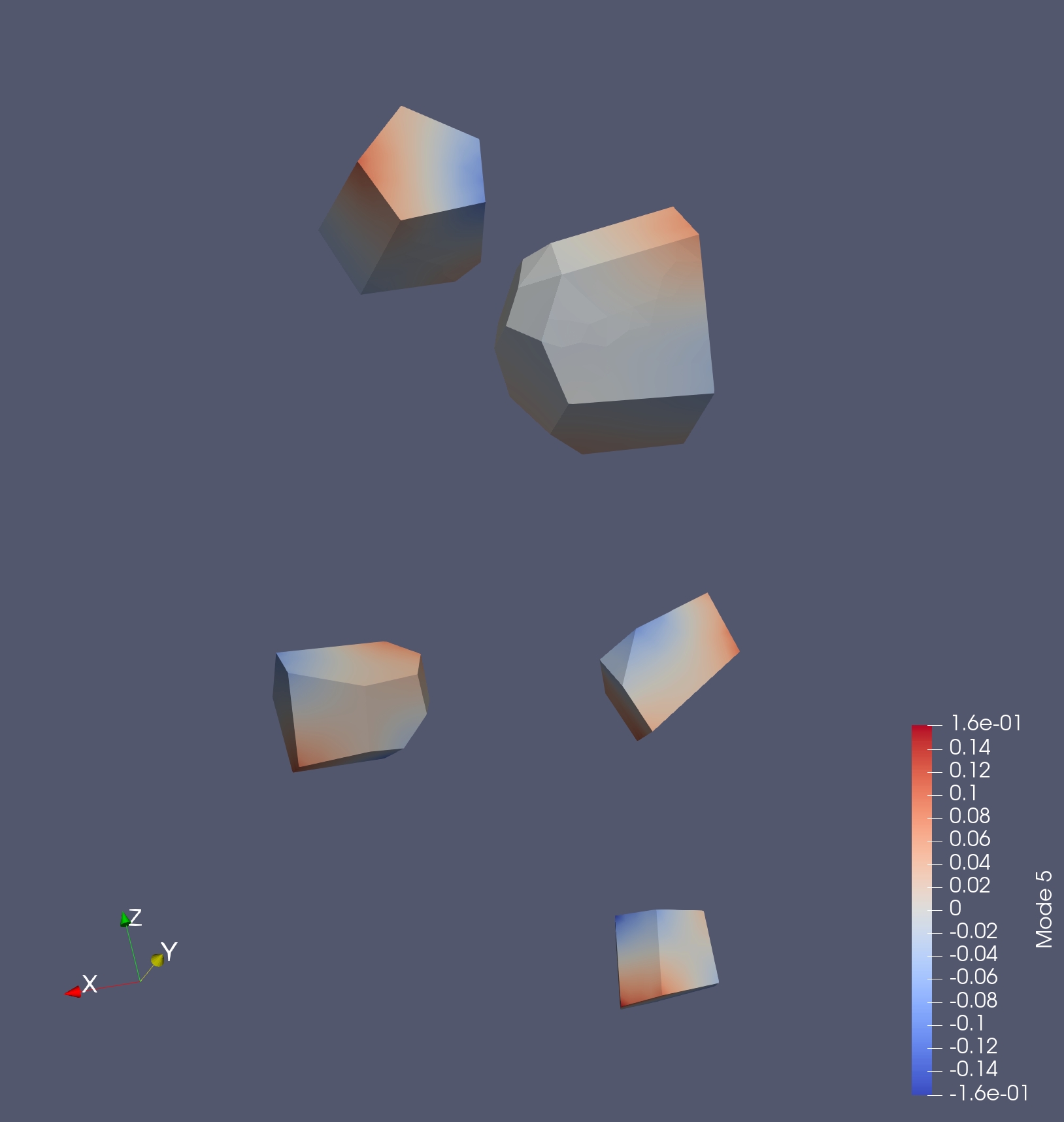
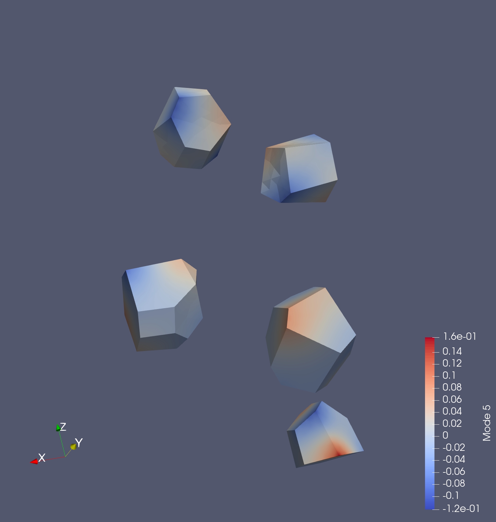
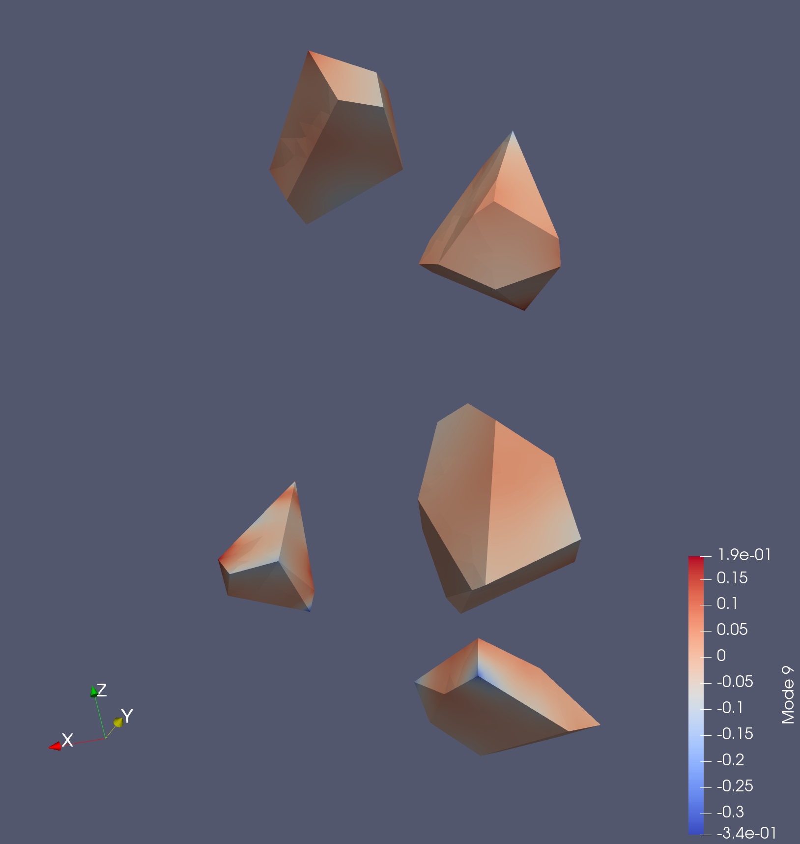
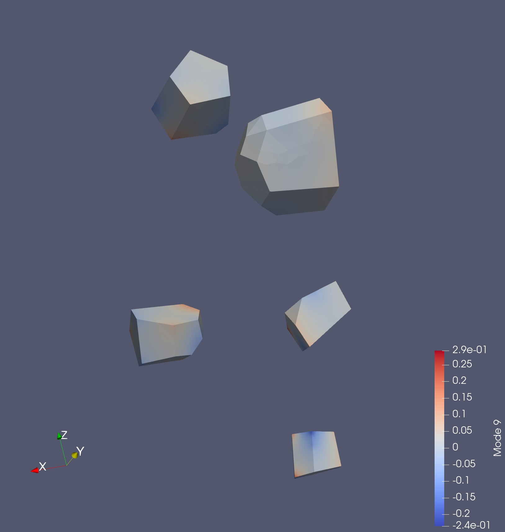
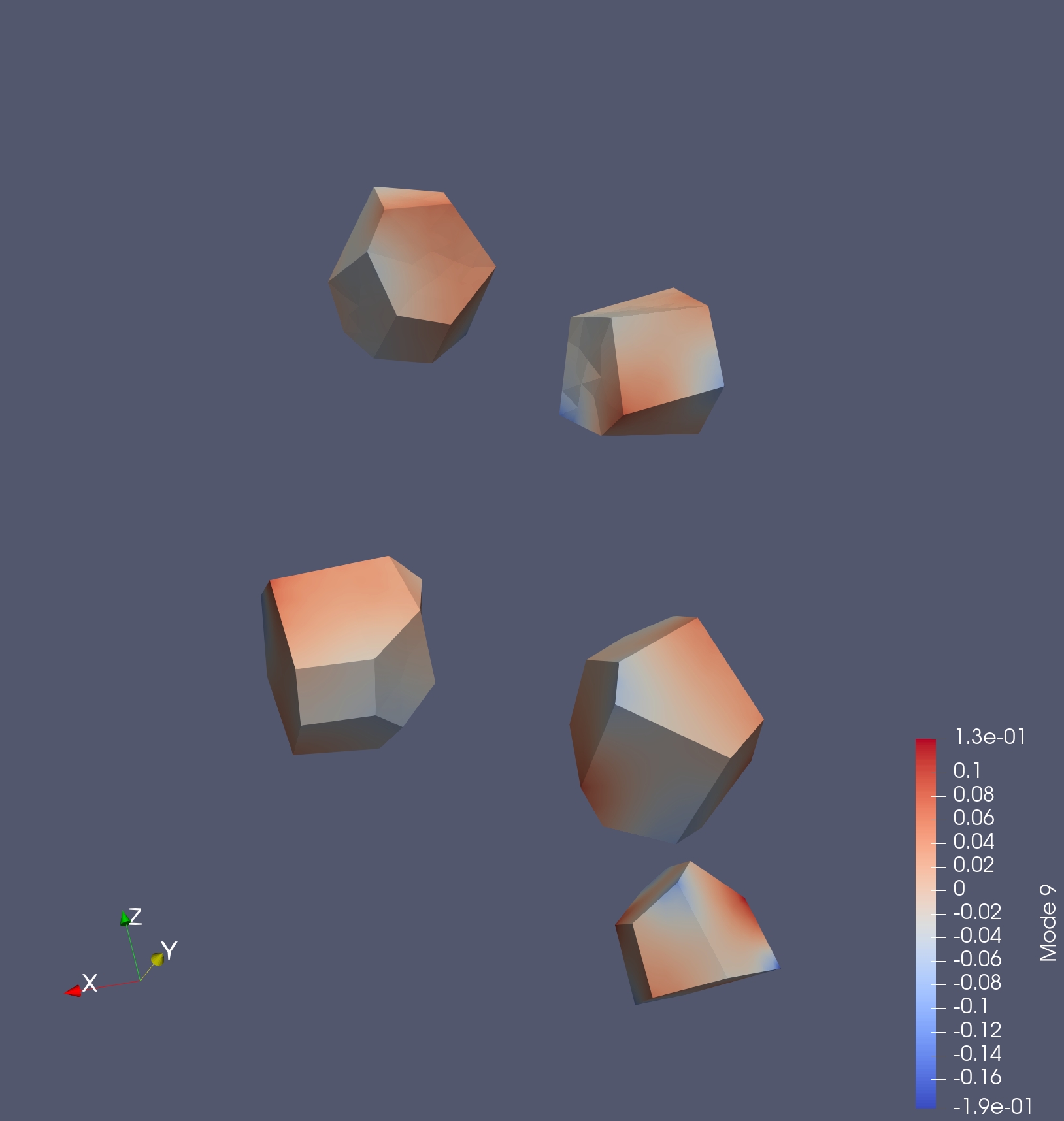
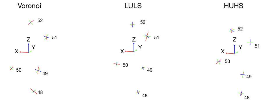
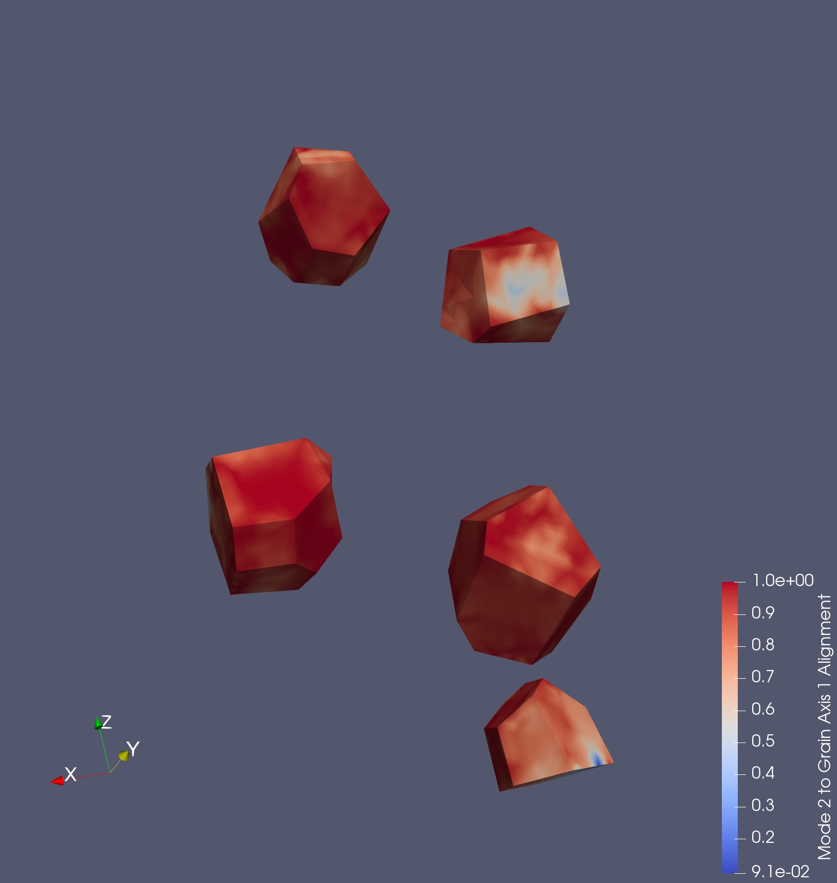
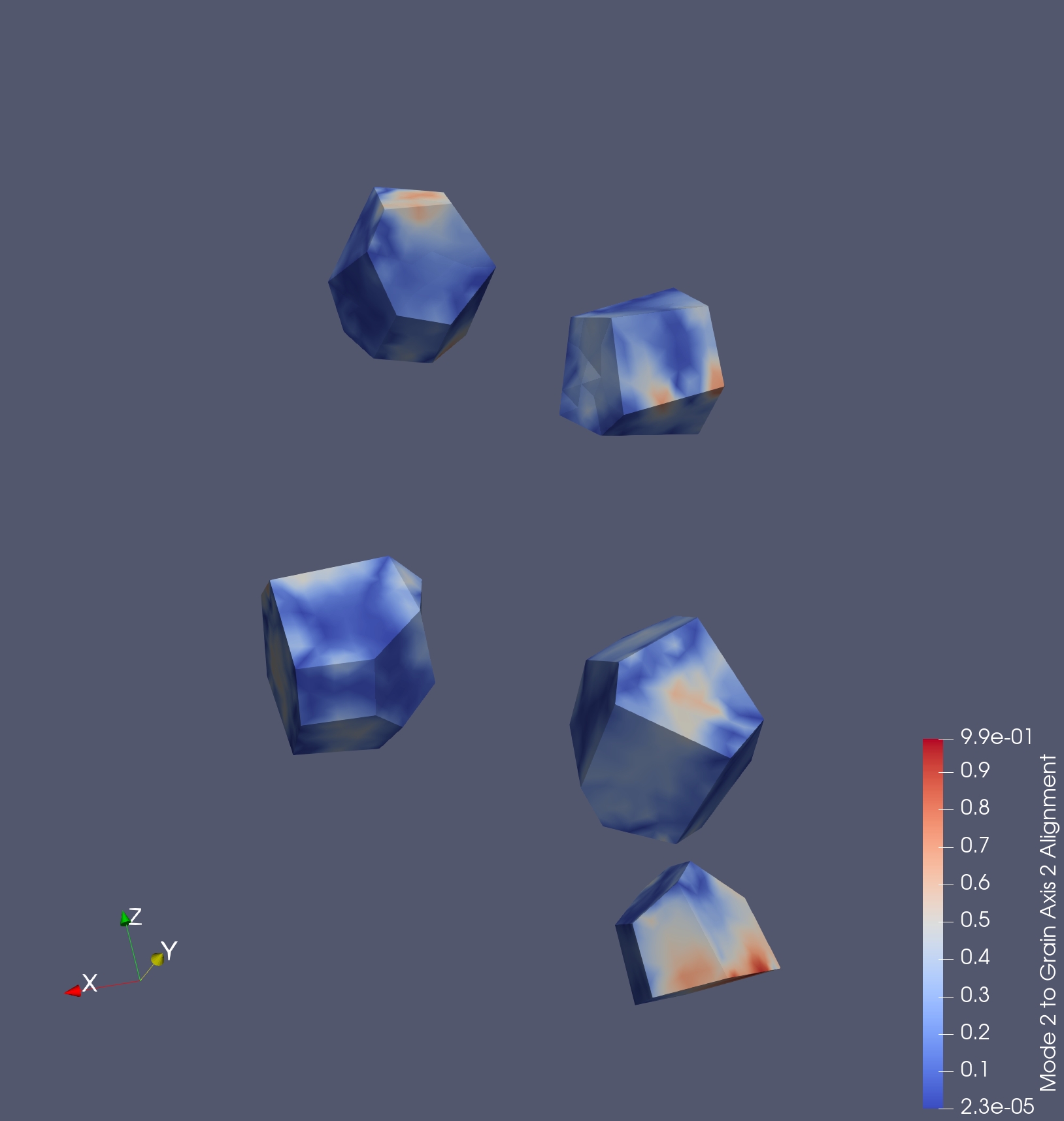
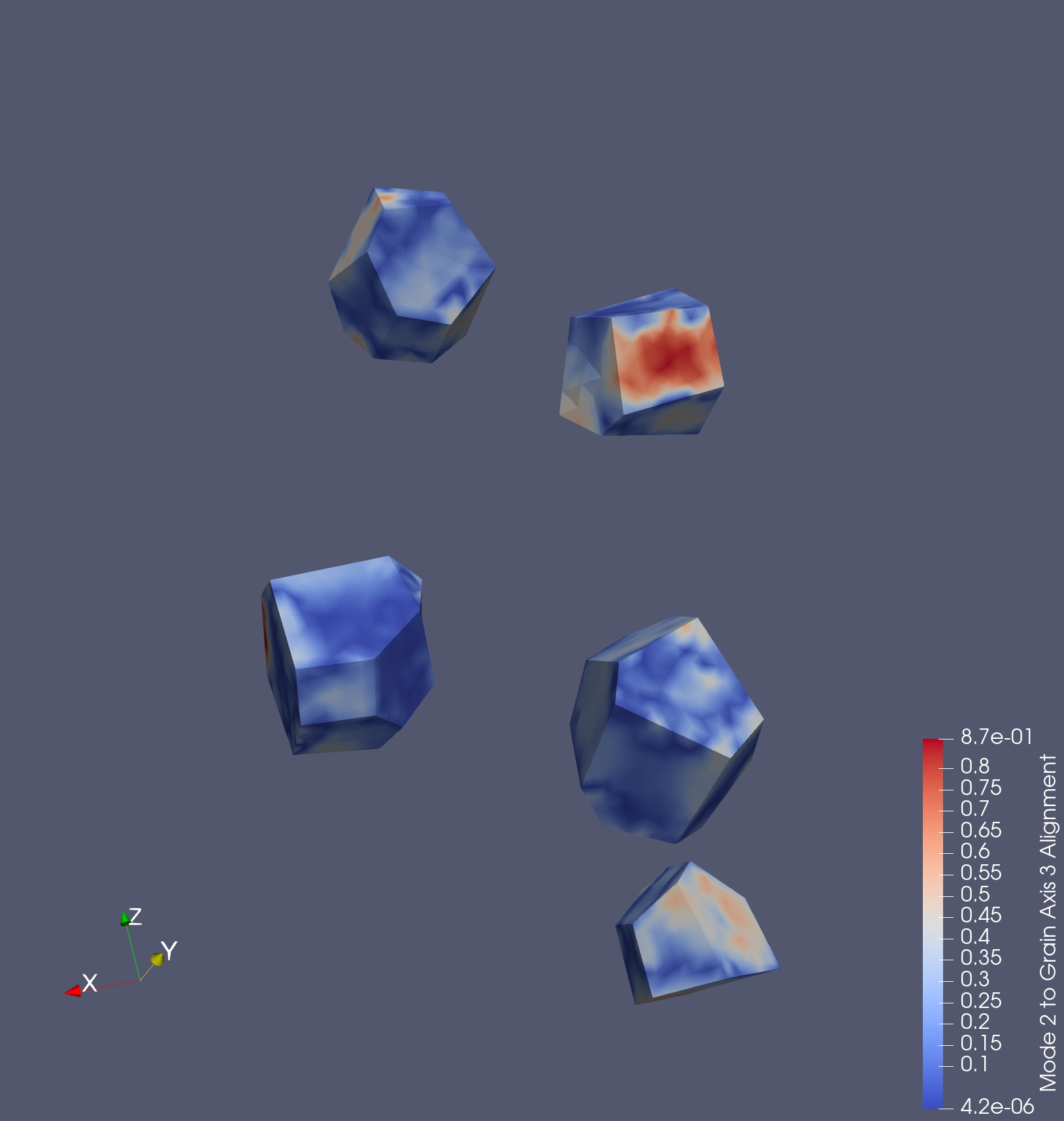
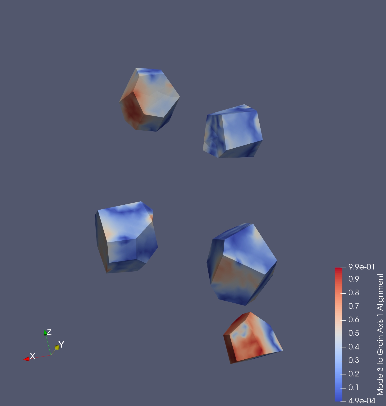
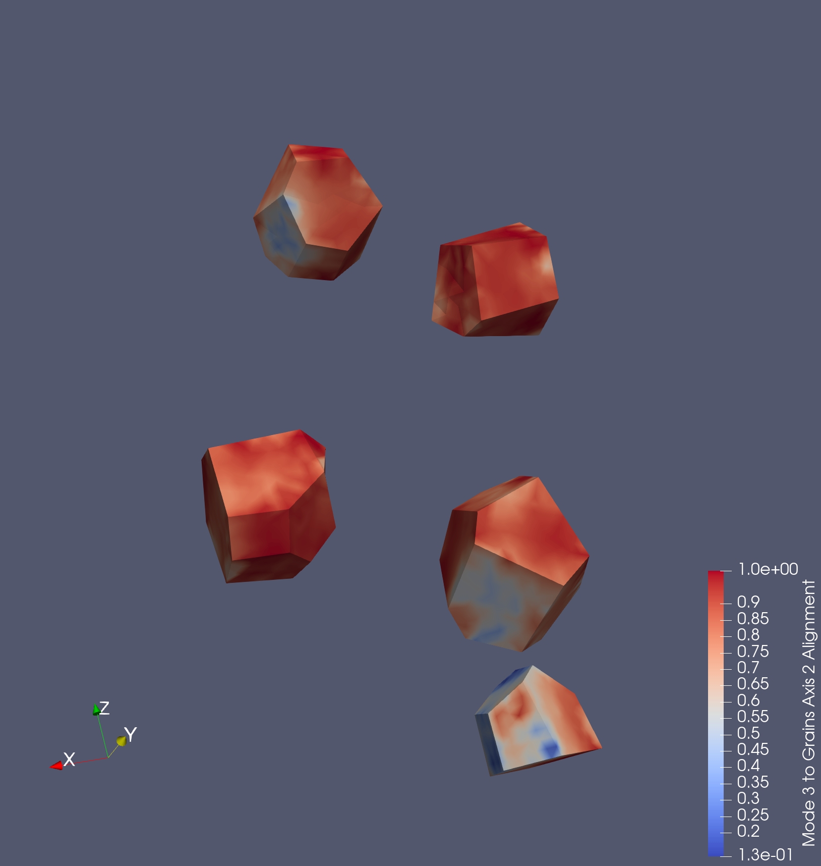
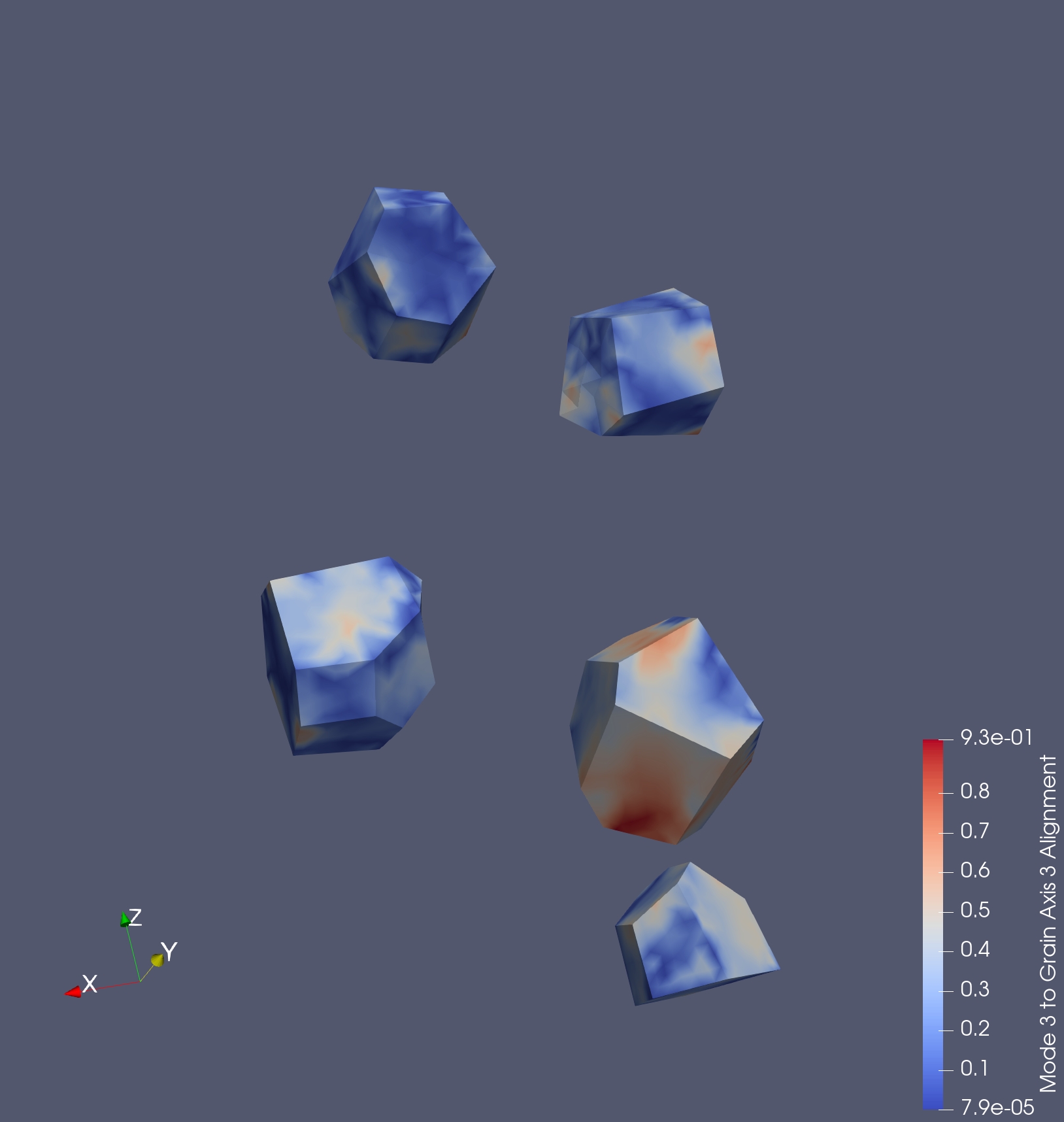
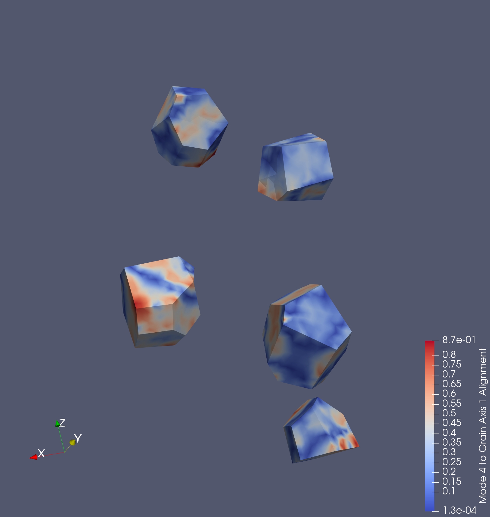
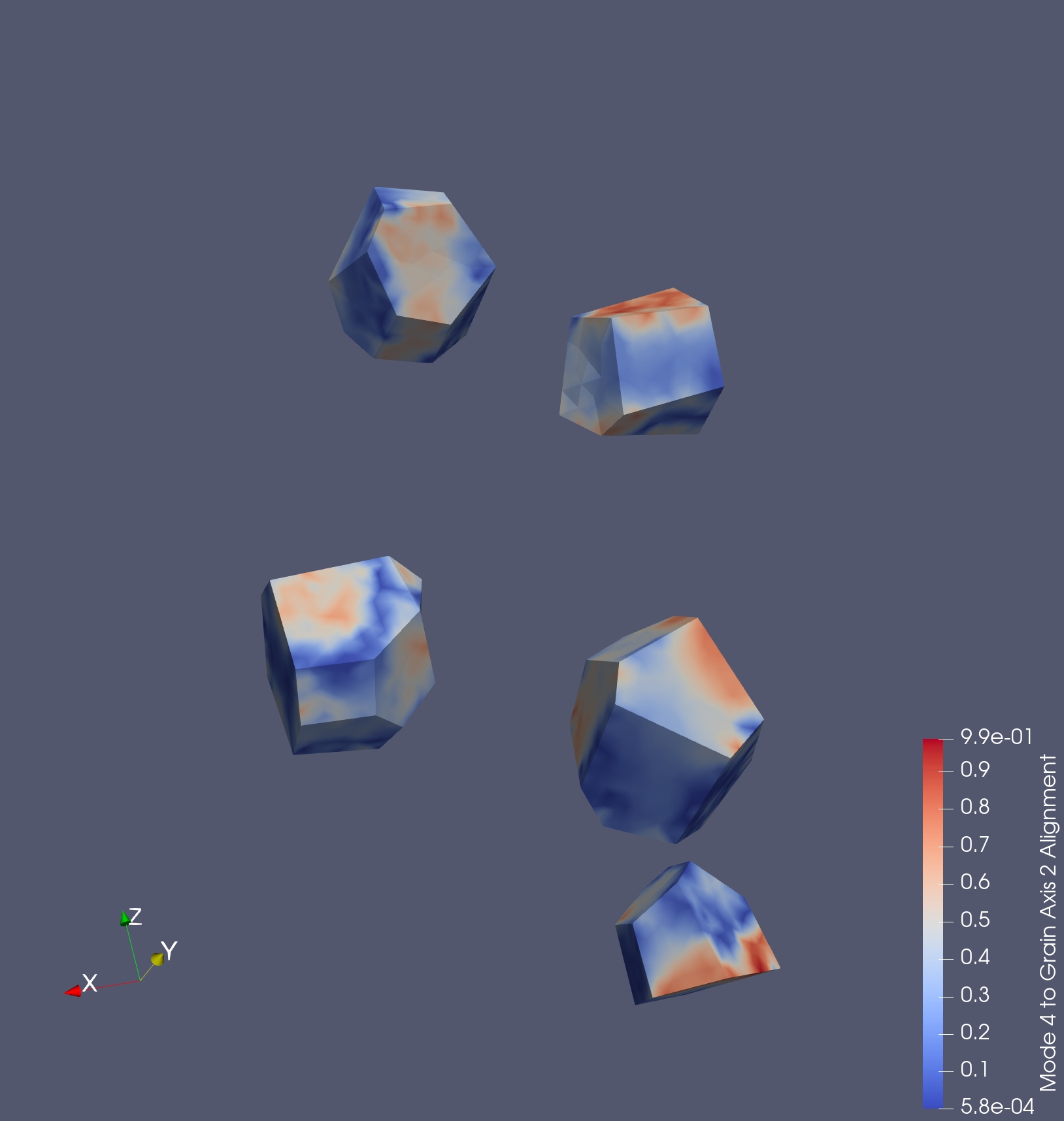
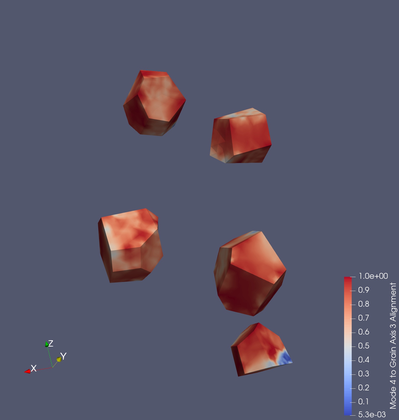
Figure 28 shows the corresponding grain axes. The alignment of Mode 2 with the Axis 1 of the grain axes is shown in Figure 29 for the HUHS sample variant. The five selected grains display the same alignment trend as the sample at-large. Figures 29 and 29 show equivalent distributions for Modes 3 and 4. Note that the for Mode 3 the alignment is strongest for Grain Axis 2 and for Mode 4 the alignment is strongest for Grain Axis 3. The other sample variants show similar trends.

Figure 28: Grain axes for Grains 48, 49, 50, 51 and 52 in: Left: Voronoi sample ; Center LULS sample; and Right HUHS sample. Axis 1: red; Axis 2: green; Axis 3: blue.

(a)

(b)

(c)

Figure 29: Alignment of the grain axes with the gradient vector of Mode 2 for the HUHS sample variant for Grains 48, 49, 50, 51 and 52 in: (a) Grain Axis 1 ; (b) Grain Axis 2; and (c) Grain Axis 3.

(a)

(b)

(c)

Figure 30: Alignment of the grain axes with the gradient vector of Mode 3 for the HUHS sample variant for Grains 48, 49, 50, 51 and 52 in: (a) Grain Axis 1 ; (b) Grain Axis 2; and (c) Grain Axis 3.

(a)

(b)

(c)

Figure 31: Alignment of the grain axes with the gradient vector of Mode 4 for the HUHS sample variant for Grains 48, 49, 50, 51 and 52 in: (a) Grain Axis 1 ; (b) Grain Axis 2; and (c) Grain Axis 3.

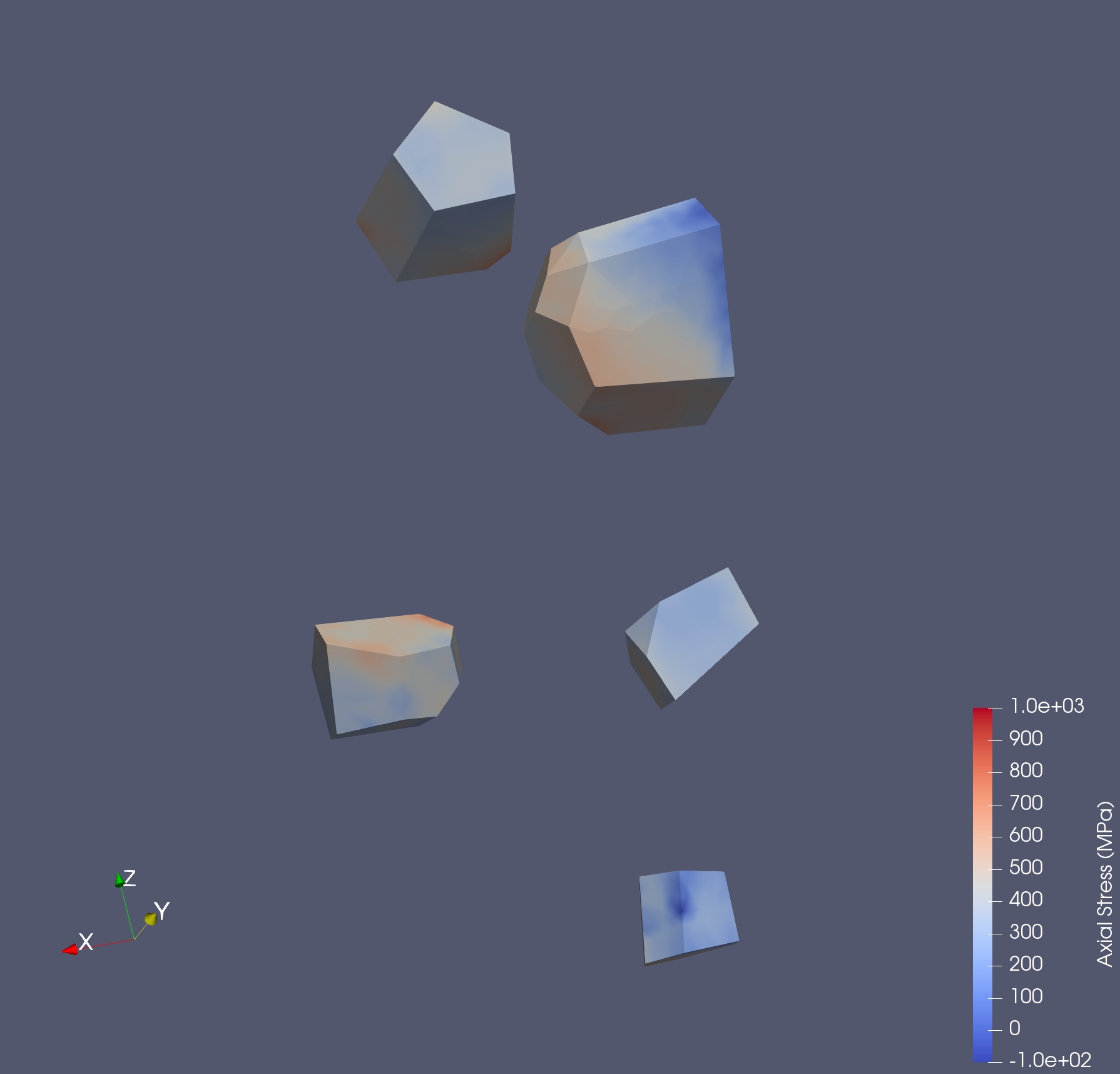
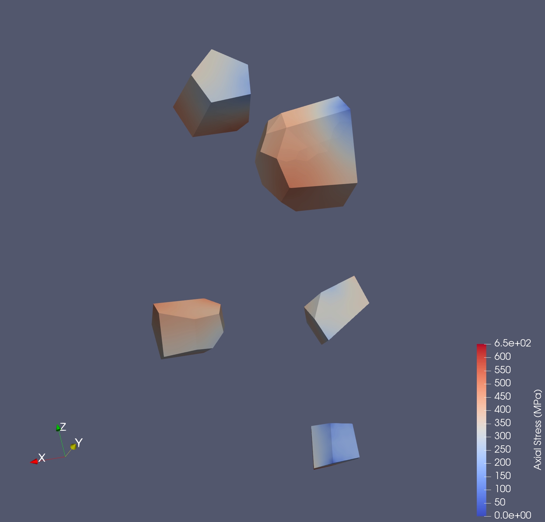
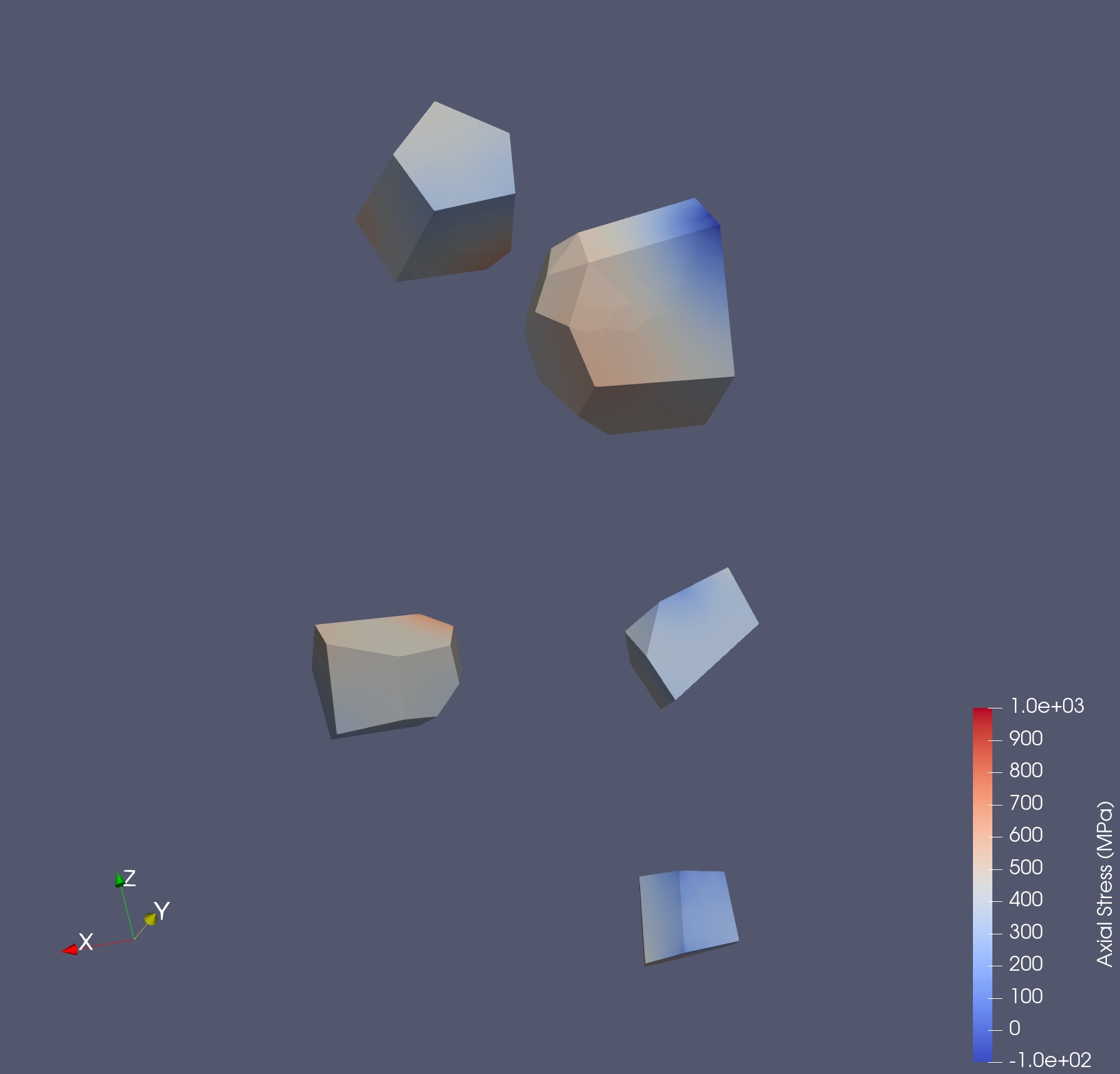
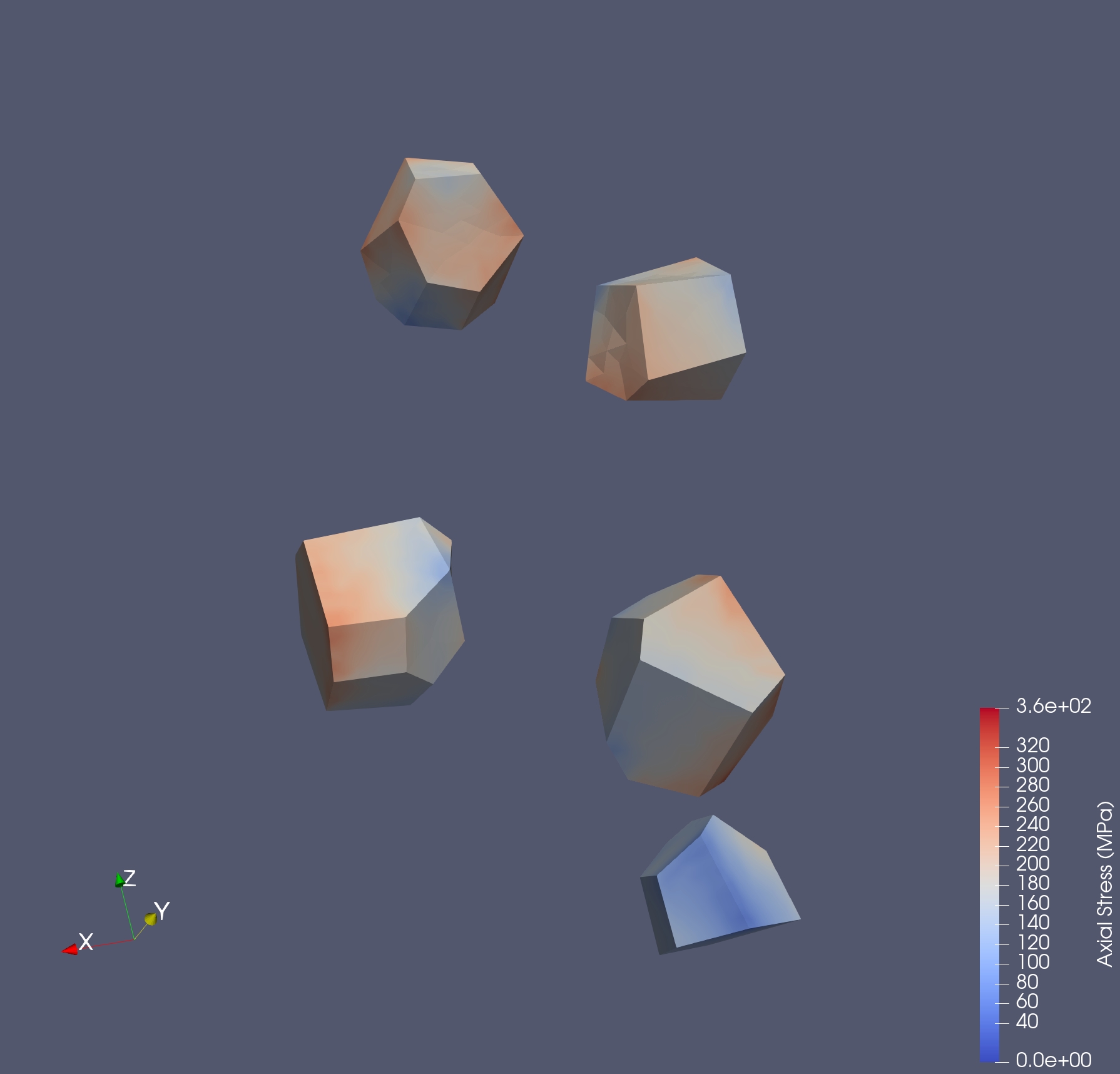
The stress distributions simulated with FEpX  and represented by harmonic fits are shown in Figures 32, 33, and 34 at nominal strains of 0.1%, 0.25% and 1.0% (0.001, 0.0025 and 0.01, respectively). The harmonic fits employ only 10 harmonic modes to approximate the simulated distributions. The fits capture the gross trends in the data, but miss on details of the distributions. As with any expansion, the fits generally improve with larger numbers of terms. Note that the inclusion of more terms (modes) does not alter the weights of the modes already employed. Rather, the overall approximation improves by means of adding corrective adjustments to the approximation. Thus we can examine the behavior of lower modes without concern that adding more modes would alter the trends regarding the weights on the lower modes.

(a)

(b)

(c)

(d)

(e)

(f)

Figure 32: Simulated axial stress distributions over Grains 48, 49, 50, 51, and 52 in the Voronoi sample at nominal strains of (a) 0.001 ; (b) 0.0025; and (c) 0.01; 10 mode fits to the simulated stress distributions at nominal strains of (d) 0.001 ; (e) 0.0025; and (f) 0.01. Note that the scales are different for the different strain levels.

(a)

(b)

(c)

(d)

(e)

(f)

Figure 33: Simulated axial stress distributions over Grains 48, 49, 50, 51, and 52 in the LULS sample at nominal strains of (a) 0.001 ; (b) 0.0025; and (c) 0.01; 10 mode fits to the simulated stress distributions at nominal strains of (d) 0.001 ; (e) 0.0025; and (f) 0.01. Note that the scales are different for the different strain levels.

(a)

(b)

(c)

(d)

(e)

(f)

Figure 34: Simulated axial stress distributions over Grains 48, 49, 50, 51, and 52 in the HUHS sample at nominal strains of (a) 0.001 ; (b) 0.0025; and (c) 0.01; 10 mode fits to the simulated stress distributions at nominal strains of (d) 0.001 ; (e) 0.0025; and (f) 0.01. Note that the scales are different for the different strain levels.

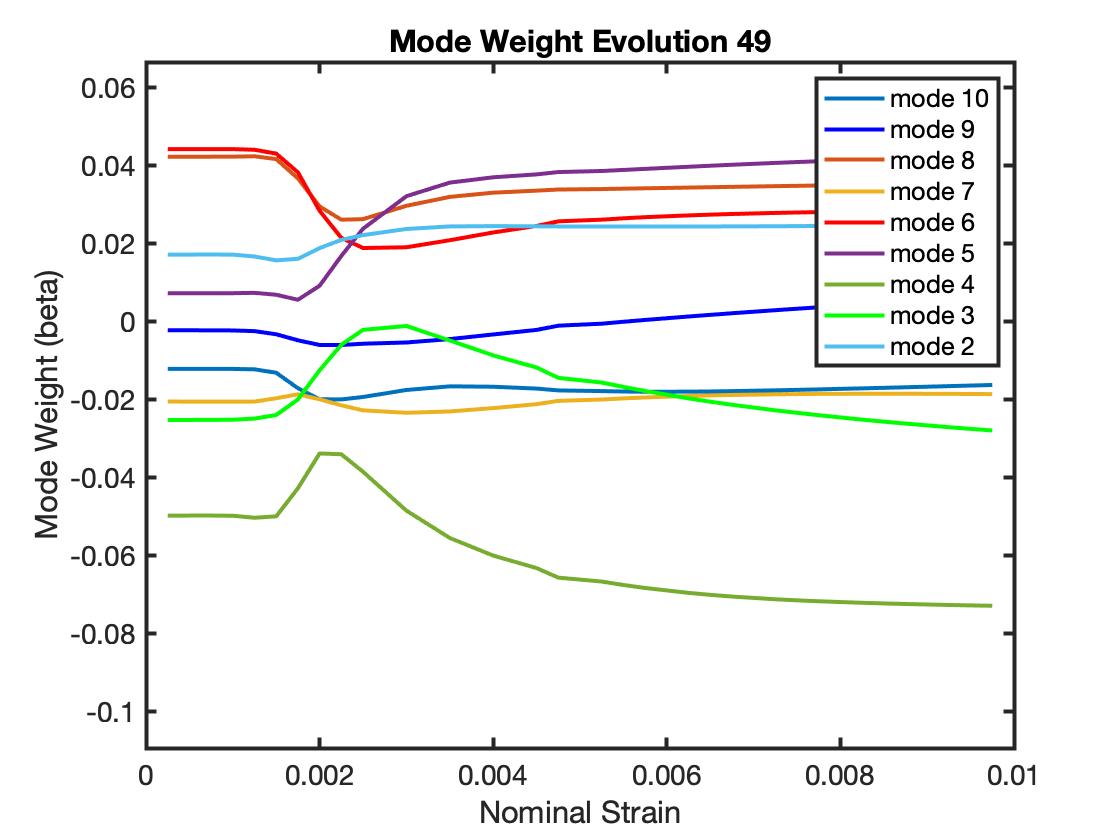
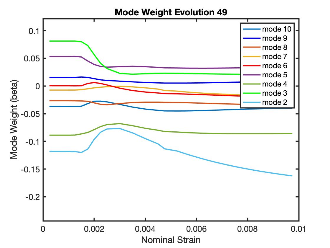
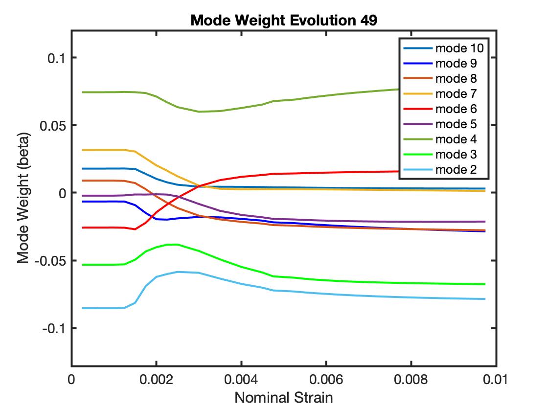
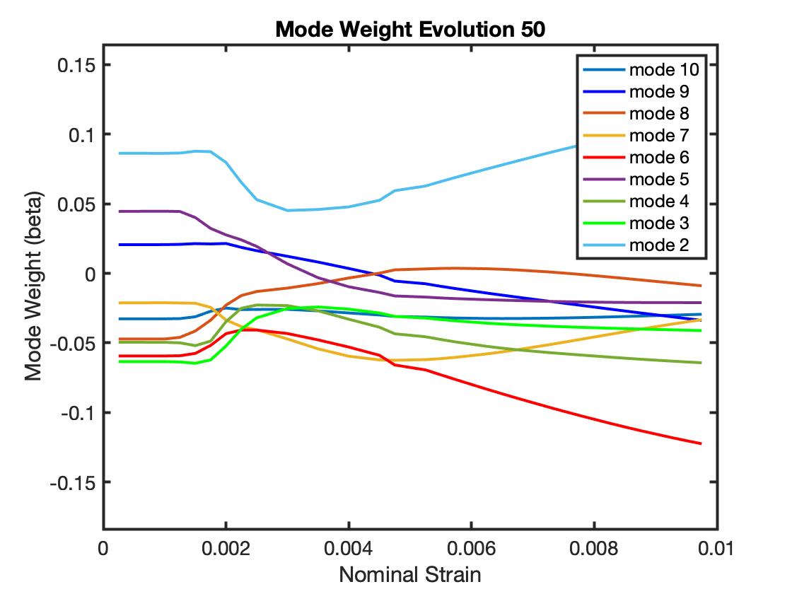
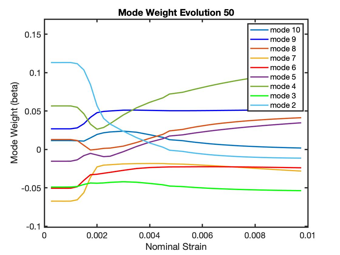
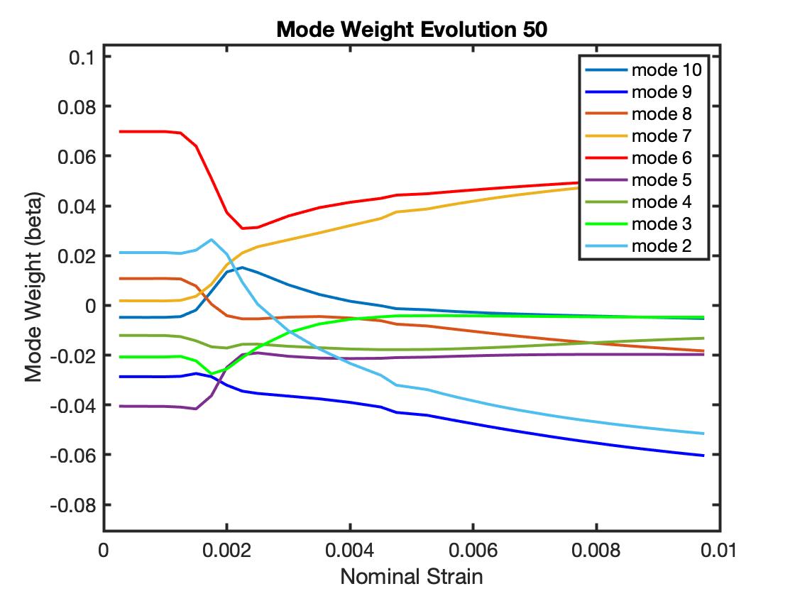
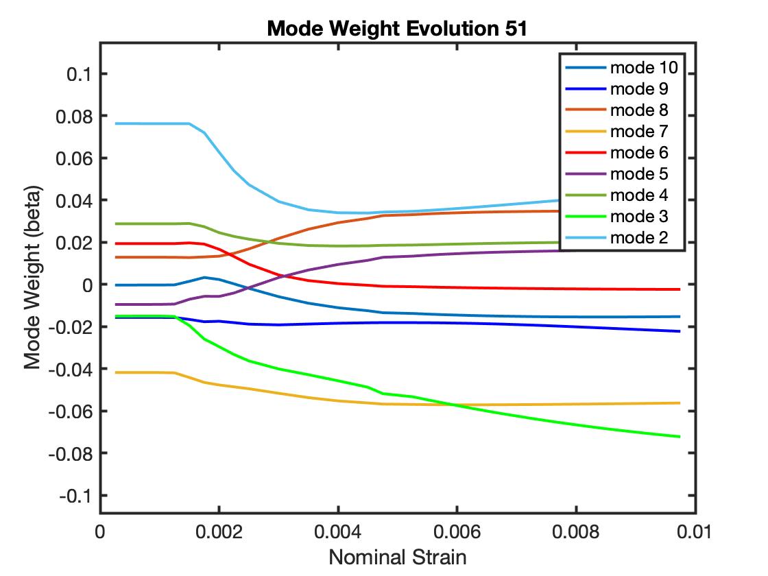
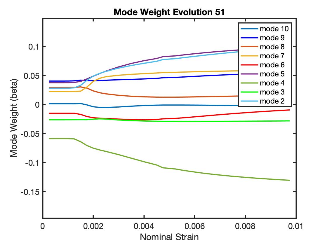
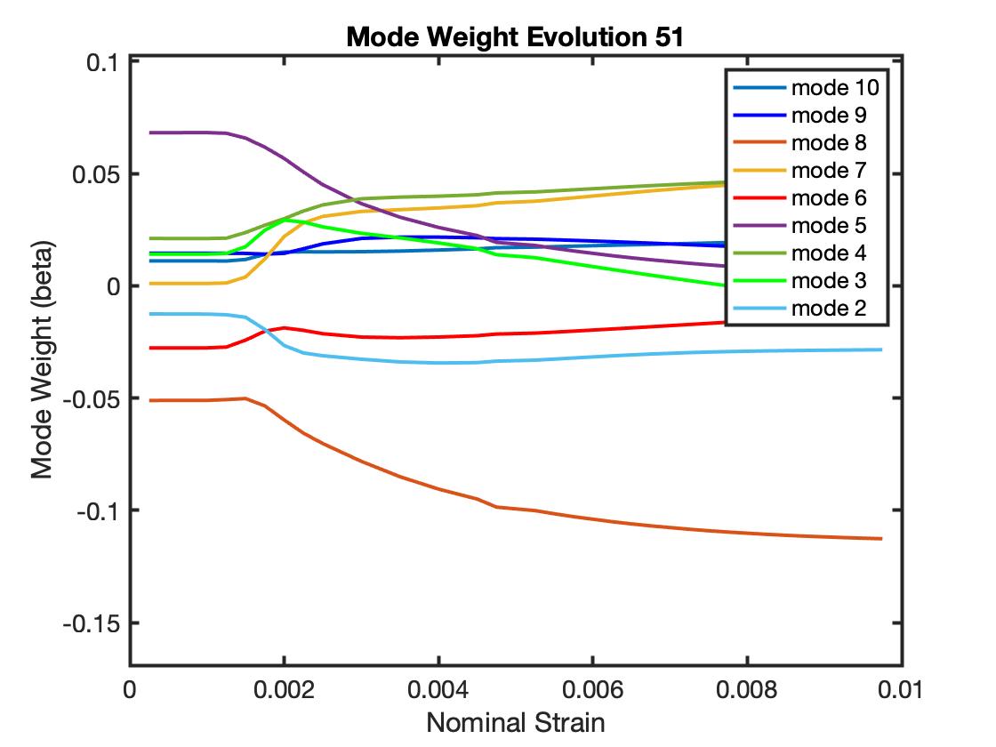
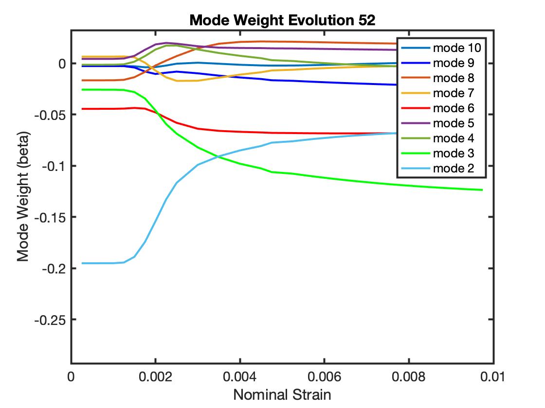
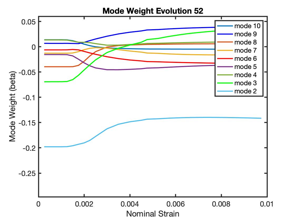
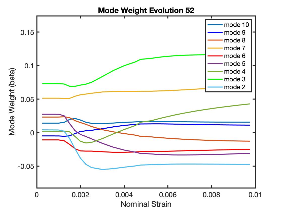
3.6 Evolution of mode weights for 5 grains

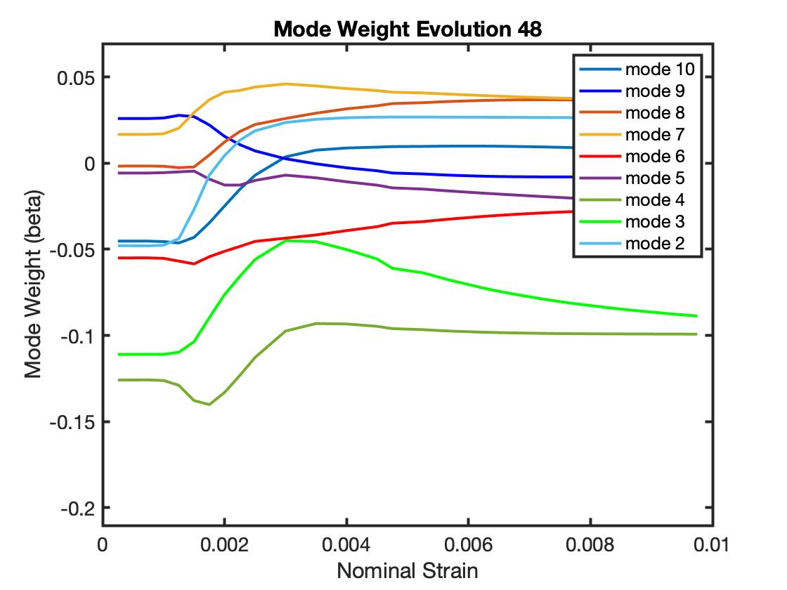
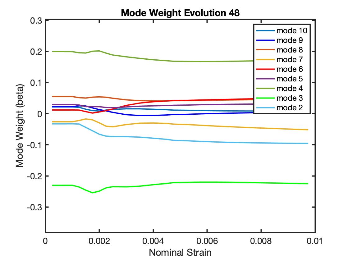
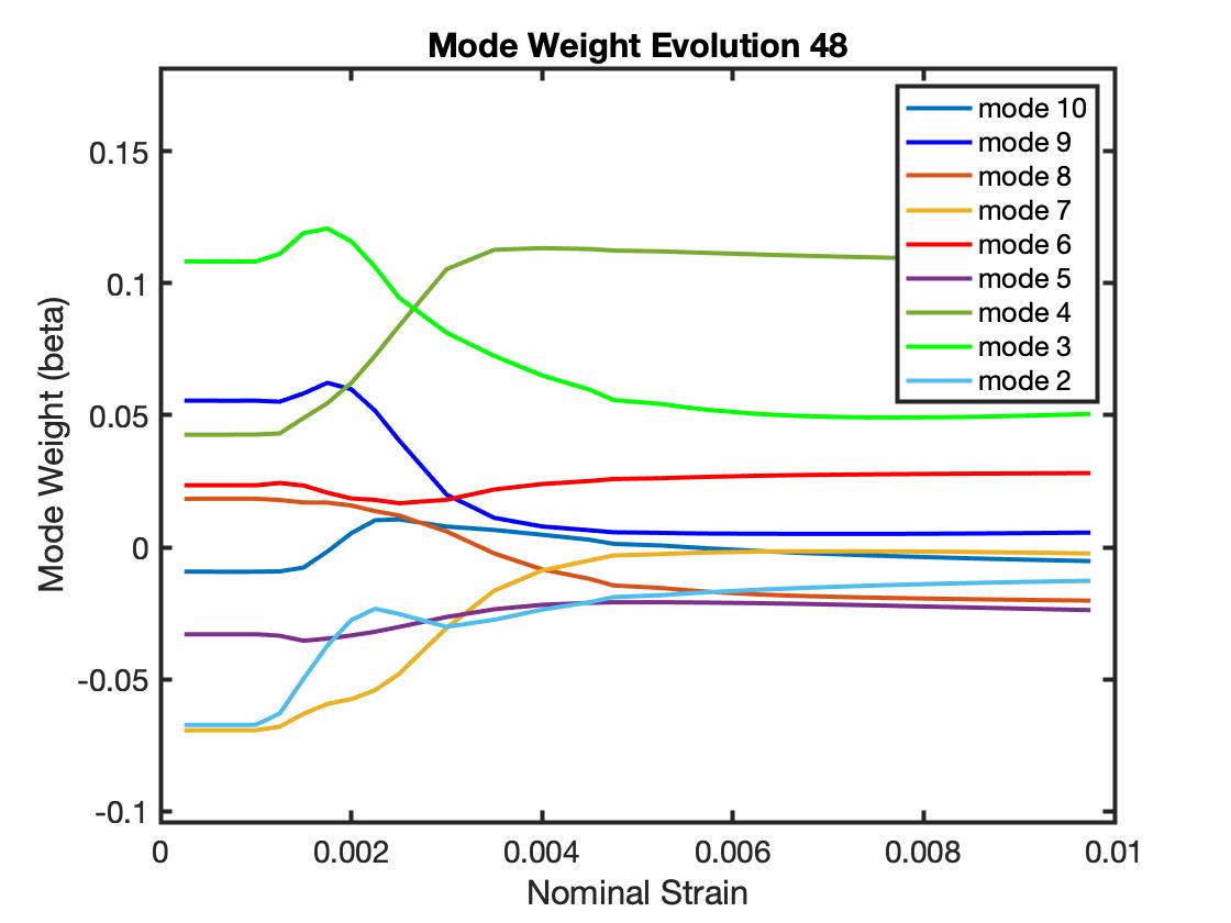
The harmonic mode weights prescribe the contribution that the associated modes add to the complete representation of the field variable. If the field variable is evolving in a manner that qualitatively alters the distribution, then the relative values of the weights change to reflect the changing distribution. This is the case with the stress when the load increases to the point that the plastic yielding initiates within grains. Prior to that point, the response remains elastic, the stress increases proportionally everywhere, and the harmonic mode weights maintain the same relative values. To illustrate this behavior, the harmonic weights are plotted versus the nominal strain grain-by-grain for the 5 grains in each of the sample variants in Figures 35, 36, 37, 38 and 39. In these plots, the evolution of the mode weights are plotted for Modes 2 to 10 after normalization by the weight of Mode 1 (the constant mode). Mode 1 increases monotonically over the loading sequence in proportion to the nominal load. The relative weights remain constant over the first several steps. The response is elastic and the stress distributions remain in the same proportion spatially. Between a nominal strain of 0.001 and 0.002, yielding initiates and the relative weights begin an evolution that continues through the elastic-plastic transition. The relative weights stabilize at a nominal strain of 0.004 to 0.005. This is more evident in some grains than others. For all grains, it holds that the ranking of the modes is different at the 0.01 strain than within the elastic regime. At 1% strain, the stress is bounded by the yield surfac – a constraint that alters the stress distributions within grains. The evolution of the mode weights serves to quantify the stress redistribution. There may be some similarity in the evolution for the same grain across samples. If true, one possible explanation lies in their sharing the same initial lattice orientation.

(a)

(b)

(c)

Figure 35: Evolution of mode weights for Grains 48 in: (a) Voronoi sample ; (b) LULS sample; and (c) HUHS sample. Note that the weights are normalized by the weight of the first (constant) mode.

(a)

(b)

(c)

Figure 36: Evolution of mode weights for Grains 49 in: (a) Voronoi sample ; (b) LULS sample; and (c) HUHS sample. Note that the weights are normalized by the weight of the first (constant) mode.

(a)

(b)

(c)

Figure 37: Evolution of mode weights for Grains 50 in: (a) Voronoi sample ; (b) LULS sample; and (c) HUHS sample. Note that the weights are normalized by the weight of the first (constant) mode.

(a)

(b)

(c)

Figure 38: Evolution of mode weights for Grains 51 in: (a) Voronoi sample ; (b) LULS sample; and (c) HUHS sample. Note that the weights are normalized by the weight of the first (constant) mode.

(a)

(b)

(c)

Figure 39: Evolution of mode weights for Grains 52 in: (a) Voronoi sample ; (b) LULS sample; and (c) HUHS sample. Note that the weights are normalized by the weight of the first(constant) mode.

4 Future work

The intent of this document is to describe the methodology used to compute discrete harmonic modes for grains of a polycrystal. The modes provide a set of orthonormal bases that may be use to represent field variables over the grains with a reduced number of parameters, namely the weights of the modes. The demonstration application illustrates the process of evaluating the discrete harmonic modes, determining the modes weights needed to represent a field variable (in this case the axial stress in a tensile loading of a sample), and tracking the changes of the weights through a deformation process that displays evolving stress distributions. No attempts are made to correlate the harmonic weights, or their changes, to attributes of the grains or the loading. We expect that discoveries are possible in both regards. MechMonics  is available via GitHub  so that researchers in addition to ourselves may pursue these.

5 Summary

The computational methods for computing sets of discrete harmonic modes in MechMonics  are presented. One set of modes is determined for each grain of a virtual polycrystal. The modes may be used to represent field data over the grain domains by means of an expansion involving weighted contributions of the modes. The procedure for evaluating the mode weights for the expansion from the field data also is presented. MechMonics  uses virtual polycrystal instantiations created and meshed by Neper. In addition to files containing the modes and their weights for designated data, MechMonics  writes output files in VTK format for visualization using Paraview  or VisIt.

A demonstration application is provided to illustrate MechMonics  capabilities. Harmonic mode representations are computed for the axial stress computed for the tensile loading of a stainless steel sample with the elastoplastic code, FEpX. Three variants or the sample are examined that differ in their grain morphologies. The differences are in the distributions of grain diameter and grain sphericity. The sample is loaded to 1% nominal strain, which is sufficient to induce plastic flow. The axial stress distributions change as the sample progresses from elastic to elastic-plastic behaviors. The evolution of the mode weights captures the evolution of the stress distributions. The sample variants show distinct histories of the mode weights stemming from the distinct size and shape metrics for each grain.

Conflict of interest

The authors declare that they have no conflict of interest.

References

- [1] Ahrens, J., Geveci, B., Law, C., Hansen, C., Johnson, C.: Paraview: An end-user tool for large-data visualization. The visualization handbook 717, 717–731 (2005)
- [2] Atkinson, K., Han, W.: Spherical harmonics and approximations on the unit sphere: An introduction (2012). Lecture Notes in Mathematics, Volume 2044, ISBN 978-3-642-25982-1 (Print) 978-3-642-25983-8 (Online)
- [3] Barton, N.R., Dawson, P.R.: A methodology for determining average lattice rotations and its application to the characterization of grain substructure. Metallurgical and Materials Transactions 32A, 1967–1975 (2001)
- [4] Childs, H., Brugger, E., Whitlock, B., Meredith, J., Ahern, S., Pugmire, D., Biagas, K., Miller, M., Harrison, C., Weber, G.H., Krishnan, H., Fogal, T., Sanderson, A., Garth, C., Bethel, E.W., Camp, D., Rübel, O., Durant, M., Favre, J.M., Navrátil, P.: VisIt: An End-User Tool For Visualizing and Analyzing Very Large Data. In: High Performance Visualization–Enabling Extreme-Scale Scientific Insight, pp. 357–372 (2012)
- [5] Dawson, P.R., Miller, M.P., Pollock, T.M., Wendorf, J., Mills, L.H., Stinville, J.C., Charpagne, M.A., Echlin, M.P.: Mechanical metrics of virtual polycrystals (MechMet). IMMI (2021). To appear
- [6] MATLAB: (R2020a). The MathWorks Inc., Natick, Massachusetts (2020)
- [7] Poshadel, A.C., Dawson, P.R.: Role of anisotropic strength and stiffness in governing the initiation and propagation of yielding in polycrystalline solids. Metallurgical and Materials Transactions A 50(3), 1185–1201 (2019). Doi:10.1007/s11661-018-5013-5
- [8] Quey, R., Dawson, P., Barbe, F.: Large-scale 3d random polycrystals for the finite element method: Generation, meshing and remeshing. Computer Methods in Applied Mechanics and Engineering 200(17-20), 1729–1745 (2011). DOI 10.1016/j.cma.2011.01.002. URL https://doi.org/10.1016/j.cma.2011.01.002
- [9] Quey, R., Renversade, L.: Optimal polyhedral description of 3d polycrystals: Method and application to statistical and synchrotron x-ray diffraction data. Computer Methods in Applied Mechanics and Engineering 330, 308–333 (2018). DOI 10.1016/j.cma.2017.10.029. URL https://doi.org/10.1016/j.cma.2017.10.029
- [10] Thompson, E.G.: An Introduction to the Finite Element Method. 1st edition. Wiley (2005)
- [11] Wikipedia contributors: Laplace’s equation — Wikipedia, the free encyclopedia (2021). URL https://en.wikipedia.org/w/index.php?title=Laplace%27s_equation&oldid=999078644. [Online; accessed 22-January-2021]
- [12] Wikipedia contributors: Singular value decomposition — Wikipedia, the free encyclopedia (2021). URL https://en.wikipedia.org/w/index.php?title=Singular_value_decomposition&oldid=1001082450. [Online; accessed 22-January-2021]
- [13] Zienkiewicz, O.C., Taylor, R.L., Zhu, J.Z.: The Finite Element Method. Its Basis and Fundamentals, 6th Edition. Elsevier Butterworth-Hienemanne, Amsterdam (2005)