Characterizing Trust and Resilience in Distributed Consensus for Cyberphysical Systems
Abstract
This work considers the problem of resilient consensus where stochastic values of trust between agents are available. Specifically, we derive a unified mathematical framework to characterize convergence, deviation of the consensus from the true consensus value, and expected convergence rate, when there exists additional information of trust between agents. We show that under certain conditions on the stochastic trust values and consensus protocol: 1) almost sure convergence to a common limit value is possible even when malicious agents constitute more than half of the network connectivity, 2) the deviation of the converged limit, from the case where there is no attack, i.e., the true consensus value, can be bounded with probability that approaches 1 exponentially, and 3) correct classification of malicious and legitimate agents can be attained in finite time almost surely. Further, the expected convergence rate decays exponentially with the quality of the trust observations between agents.
I Introduction
In this paper we address the problem of multi-agent distributed consensus in the presence of malicious agents. The consensus problem is of core importance to many algorithms and coordinated behaviors in multi-agent systems. It is well-known however, that these algorithms are vulnerable to malicious activity and/or non-cooperating agents [1, 2, 3, 4, 5] and that several of the existing performance guarantees for the nominal case fail in the absence of cooperation [6, 7].
Many works have investigated the possibility of attaining resilient consensus, or consensus in the face of non-cooperating or malicious agents. However, achieving resilience often relies on conservative assumptions of connectivity, and bounds on the maximum number of malicious actors. A classical result for consensus in networks with non-cooperating agents (faulty or malicious) holds from [1, 6]:
Well behaving agents can always agree upon a parameter if and only if the number of malicious agents is less than 1/2 of the network connectivity.111The connectivity of a graph is the maximum number of disjoint paths between any two vertices of the graph.
This result has long been held as a fundamental requirement for achieving consensus in unreliable networks [1, 6, 8].
For purely cyber systems, where data is used to validate information, these limitations are difficult to circumvent. Cyberphysical systems (CPS) however, are becoming prevalent in many fields, from robotics to power systems to traffic systems and beyond [9]. These systems provide new opportunities to additionally use physical channels of information for data validation. This physical channel data can be exploited to understand “trust”, or the trustworthiness of data, among the agents in the system. Examples include using observers to compare against system models [10, 11], using camera or other physical channel data [12], or using transmitted communication channels by comparing against a known carrier signal to find whether a message has been manipulated [13, 14]. Wireless channels are of particular interest since they often exist in multi-agent systems as a medium for information exchange and can also be used to extract useful information such as, for example, tracking motion [15, 16], localizing robot agents [17, 18], as well as providing security to wireless systems [19].
Our recent work in [20] derives the characterization of a stochastic value of trust, , that approaches 1 for trusted transmission and 0 for an untrusted transmission between any two agents and in the case of a Sybil Attack. Importantly, these recent results show that information capturing the trustworthiness of communicating agents can be obtained from analyzing the communication signals themselves - alluding to the fact that the probability of trust between agents can be characterized using information that already exists in multi-agent networks.
However, there remains a need for a unified mathematical framework to guide how a probabilistic understanding of trust between agents can be used to arrive at important performance guarantees for resilient coordination and consensus.
We are motivated by these recent works to derive consensus results that take trust into account. This paper provides a unified framework that characterizes the value of trust when it comes to achieving resilient consensus in adversarial settings.
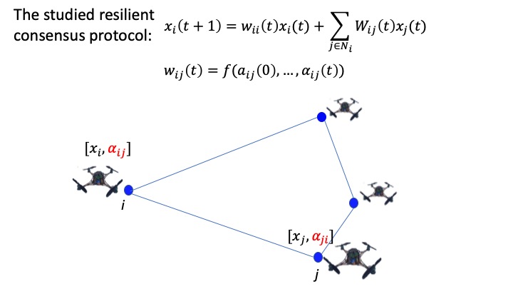
We generalize the concept of trust between agents by considering the availability of stochastic observations that can be thought of as a probability of trust between any two agents and in a system (see Fig. 1). We show that using this additional information can lead to strong results for resilience. Namely, under certain conditions on that we characterize, we establish the following results:
1) Convergence: We show that convergence to a common limit value is possible almost surely, even when the number of malicious agents is larger than less than 1/2 of the network connectivity.
2) Deviation from nominal average consensus: Whereas without additional information of trust between agents the presence of malicious agents comprising more than 1/2 of the network connectivity could take the consensus value to any limit, we show that by using ’s, the influence of malicious agents can be bounded and that this bound can be characterized.
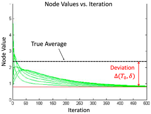
3) Convergence rate: We show that convergence can be attained in finite time with arbitrarily high probability, and that the expected convergence rate decays exponentially with the quality of the observations and other problem parameters that we characterize.
A roadmap of our paper is as follows: We begin by providing some background and context for the resilient consensus problem in Section I-A. In Section II we present our consensus model, our model of trust between agents and the observations, and we characterize the influence of malicious agents on multi-agent consensus. In Section III we provide our theoretical results and analysis of convergence, deviation, and the convergence rate for consensus with malicious agents. Finally, in Section IV we present simulation results, followed by Section V that provides a discussion and future work directions, and a conclusion in Section VI.
I-A Related Work
The problem of coordination in multi-agent systems and consensus has a long history [21, 22, 23, 24]. In particular, the consensus problem has enjoyed the development of many fundamental results providing insights into conditions for convergence [25, 26, 27, 28, 29], convergence rate [30, 31, 32], and general analysis and implementation [33, 34]. Similarly, in the current paper we hope to start building a more general mathematical foundation for resilient consensus using the concept of inter-agent trust.
Resilient consensus refers to consensus in the case where agents are non-cooperative either due to faulty or malicious behavior. This is an important problem due to the prevalence of the non-cooperative case. For multi-robot systems for example, security is of utmost importance as these robot systems enter the world as autonomous vehicles, delivery drones, or partners in security and defense [35, 36, 37]. For cyberphysical systems the issue of security is a highly investigated topic due to the increasing role that cyberphysical systems play in critical infrastructure such as power grids, traffic management systems, and beyond [38, 39, 40, 41, 42, 43]. As a result, there has been increased attention on exposing the vulnerabilities of consensus in multi-agent systems [1, 2, 3, 4] and on developing new theory to support resilient consensus for these systems [6, 5, 8, 44, 10]. A common theme in these works is to use transmitted data to identify and thwart attacks, and as a result they are often accompanied by important constraints on the minimum connectivity needed in the graph or requirements on the maximum number of malicious agents that can be tolerated. Take for example the classical result from [1] which states that well behaving agents can always agree upon a parameter if and only if the number of malicious agents comprises less than 1/2 of the network connectivity. Additionally, the work [8] presents conditions for an asymptotic convergence to an arbitrary point in the convex hull of the initial values of the legitimate agents.
Cyberphysical systems, including multi-robot systems as a prominent example, offer more physical channels of information that can be used for data validation and for quantifying “trust” between agents (robots, sensors, autonomous vehicles, and more). Camera data, communicated wireless signals, lidar, and radar, are a few examples of physical channels of information that often exist in cyberphysical systems and can be used to validate data transmitted between agents. Indeed, many works have exploited the physics of cyberphysical systems to validate transmitted data which presents great promise for the security of these systems [12, 45, 13, 11, 46, 14].
Advances in sensing using wireless signals is especially promising in this domain as many multi-agent systems transmit messages over a wireless medium [47, 48]. The wireless community has demonstrated that these wireless signals themselves contain important information that can be fruitfully exploited for security. For example it has been shown that wireless signals can be analyzed to provide tracking and localization of agents [49, 18, 15, 50, 16, 51], authentication [19, 52, 53], and thwarting of spoofing attacks [54].
Deriving Trust Values using Wireless Signals: Here we provide some intuition on one particular example of quantifying trust between agents by exploiting physical channels of information; specifically, using wireless channels. Our previous work developed a method for measuring directional signal profiles using channel state information (CSI) from the wireless messages over each link in the network [55, 50]. These profiles measure signal strength arriving from every direction in the 3D plane. Directional signal profiles display two important properties: 1) transmissions originating from the same physical agent have very similar profiles and 2) energy can be measured coming from the direct-line path between physical agents. The paper [20] quantifies these properties, providing an analysis that shows both analytically and experimentally, that a single scalar value (shifted by -0.5 from [20]) can be computed for each signal profile that quantifies the likelihood that the transmission is coming from the same physical (spoofed) node, or a unique (legitimate) node; a property critical for thwarting Sybil Attacks. Intuitively, the was shown experimentally and theoretically to be close to -0.5 if one of the agents is a spoofed node and close to 0.5 if both agents are legitimate nodes in the network [20]. This is captured quantitatively by the bounds on the expectation of the . The current paper takes inspiration from this previous work which shows the existence of such variables for stochastically characterizing trust between agents, but goes beyond to define a unified mathematical framework for using trust to obtain certain performance guarantees for consensus in multi-agent systems. As such, Definition II.2 specifies the mildest characteristics of such as term in order to achieve strong performance guarantees. Thus the results contained herein would be compatible with stochastic variables as derived in [20] or any other physical channels that satisfy Definition II.2. We note however, that the focus of this paper is not on the derivation of stochastic trust values. Rather, we focus on the development of the mathematical foundations for why and how such values can be key to achieving certain performance guarantees that would be difficult or impossible to obtain otherwise.
Contributions in the context of previous work: This paper builds most closely off of our previous work in [20, 56] which shows that a stochastic variable can be extracted from wireless signals between agents to verify the validity of an agent’s identity (in a probabilistic sense) during a Sybil Attack. Further, [56, 57] shows the potential of using these values to arrive at resilient consensus. In the current work we assume the availability of such probabilistic observations of trust between agents, the , and focus on the development of the mathematical machinery that can utilize these trust values to arrive at strong results for resilient consensus. Key differentiating results include: 1) We provide convergence rate results for the case where the number of malicious agents is larger than 1/2 of the network connectivity, showing that convergence in finite time is possible with arbitrarily high probability. To the best of our knowledge, this is the first time that this result has been formally proven. 2) We divide the consensus algorithm into two critical stages with broad consequences for the attainable performance guarantees. In the first stage the agents observe the network, i.e. they collect values of to detect malicious agents but do not start running the consensus protocol. In the second stage, agents continue to collect values of and also adapt their data values using a modified consensus protocol that includes received data only from agents they classify as trustworthy. We show that the impact of observing the network for some time window is highly consequential for deviation and convergence, where convergence rate and deviation amount decreases exponentially with increasing . 3) We use weights that define a switching topology allowing for arbitrarily small deviation in the final consensus value. 4) The current work allows for the use of non-symmetric weights which can accommodate larger classes of multi-agent systems. Finally, the results in this paper are general to many classes of attacks so long as certain characteristics on the probability of trust between agents, , are met. We establish these key characteristics and define their roles in convergence, deviation, and convergence rate to consensus.
II Problem Description
We consider the problem of consensus for multi-agent systems. The agents in the system communicate over a network, which is represented by an undirected graph, , where denotes the set of node indices for the agents and denotes the set of undirected edges. We use to denote the edge connecting agents and . The set of neighbors of node is denoted by . Note that by this definition if is neighbor of , then is also a neighbor of . With the graph , we will associate time-varying nonnegative weights , which capture the information exchange process among the agents at a given time . We use to denote the th entry of the weight matrix . For these matrices, we have and only if , and otherwise. In this way, the positive entries of the matrices are associated only with the edges in the set . Additionally, the matrices need not be symmetric. We consider the case where a subset of nodes with indices denoted by the set , , are either malicious or malfunctioning and, thus, do not reliably cooperate in the consensus protocol. The set is assumed to be unknown, with the cardinality . An agent that is not malicious or malfunctioning is termed legitimate, and the set of legitimate agents is denoted , , with the cardinality .
In what follows, we use to denote the zero matrix, where the dimension of is to be understood from the context. We say that a matrix is nonnegative if its entries are nonnegative, i.e., for all , and we write to denote that is nonnegative. We write to denote a matrix having all entries positive, i.e., for all . A nonnegative matrix is row-stochastic if the sum of its entries in every row is equal to 1, and it is row-substochastic if the sum of its entries in every row is equal to or less than 1. We use to denote the vector with all entries equal to 1. Given a vector , we use or (when has a subsrcipt) to denote its th entry. A similar notation is used for the entries of a matrix.
II-A The Model
We are concerned with the problem of consensus where each legitimate agent updates its value according to the following update equation (see [5]) for all ,
| (1) |
where , while the weights are nonnegative and sum to 1, i.e., , for and . The process is initiated at some time with the agents’ initial values for all .
Definition II.1 (Malicious agent).
Agent is said to be malicious if it does not follow the rule in (1) for updating its value at some time .
Let denote the vector of values for all the agents at time . Without loss of generality, we assume that the agent indices are ordered in such a way that the vector can be separated in two components; the first component representing the legitimate agent values and the second component representing the malicious agent values . In this way, the consensus dynamics takes the following form:
| (2) |
where is the matrix multiplying the state component corresponding to the legitimate agents’ values, and is the matrix multiplying the state component corresponding to the malicious agents’ values. The matrices and dictate the dynamics of the malicious agents’ values and are assumed to be unknown. For the sake of simplicity, we assume that a malicious agent sends the same data value to all of its neighbors, however, our analysis holds for the case where a malicious agent can send different data values to different neighbors at each iteration. We consider the case when a parameter is known to all legitimate agents and it is known that the values should not exceed at any time. The assumption for all and , is reasonable, since an agent can be classified as malicious based on its value (i.e., if at some time ). Thus, in this paper, our focus is on the update rule in (2) where for all and time instants .
In this paper we are interested in the case where each transmission from agent to agent can be tagged with a random observation of a random variable . The random variable represents a probability of trust that agent can give to its neighbor .
Definition II.2 ().
For every and , the random variable taking values in the interval represents the probability that agent is a trustworthy neighbor of agent . We assume the availability of such observations throughout the paper.
We refer to [20] for an example of such an value. Intuitively, a random realization of contains useful trust information if the legitimacy of the transmission can be thresholded.
In this paper we assume that a value of indicates a legitimate transmission and indicates a malicious transmission in a stochastic sense (misclassifications are possible). Note that means that the observation is completely ambiguous and contains no useful trust information for the transmission at time .
Our ultimate goal is to understand the convergence, and convergence rate properties of consensus under the influence of a malicious attack if such observations of trust are available. Toward this goal, our first objective is to construct the appropriate weight matrix for legitimate agents’ state dynamics in (2) by using some function of the observations , where is a legitimate agent so that and is a neighbor of so that . In this way, the legitimate agents’ ability to isolate the malicious agents is reflected in the convergence of the weight matrices to the zero matrix and the convergence of the weight matrices to a row-stochastic matrix, where the convergence is in a probabilistic sense (to be defined shortly). Necessary characteristics of to allow for the convergence of the linear protocol in (2), possibly including its distribution, bounds on expectation, etc., will be derived in this work.
In line with this model, in addition to broadcasting its value at each time , we assume that a message from each agent is tagged with an observation for every neighboring agent , i.e., (see Figure 1). The purpose of this work is to develop the necessary properties of such that consensus can be maintained in the presence of malicious or malfunctioning agents.
Suppose that, in the interval of time , the legitimate agents only use their measurement of the trustworthiness values , , . We refer to this interval of time as an observation window where agents can amass a history of trust values before starting the consensus. At time , the agents start the data passing phase with the weights , where is some function capturing the history of all observations and denotes the indicator function. Our goal is to study the resulting consensus dynamics over time. Since we start the consensus algorithm (2) from time , we have that for all .
Let denote the backward product of the matrices , i.e.,
where denotes the identity matrix. Following (2) the value of the legitimate agents at any point in time has two salient influence terms, the values contributed by other legitimate agents and the values contributed by other malicious agents so that for all
| (3) |
where
| (4) |
and
| (5) |
Relation (3) shows explicitly how the states of legitimate agents depend on their initial states at time and on the states of malicious agents. The term given in (5) captures the total influence of the malicious agents on the states of the legitimate agents from the initial time to the current time and will be the primary subject of study. Specifically, we will study attainable bounds on the malicious agents’ influence term .
Remark (Arbitrary starting time of the consensus.).
We emphasize that the consensus updates from Eq. (2) begin at an arbitrary time and that before this time agent values are not updated for . In other words, for only observations are collected by each agent for its neighbors . The choice of is a user-selected parameter that affects the overall influence of malicious agents in the network and the convergence rate according to a relationship that we later characterize.
We now construct a modified weight matrix that governs the state dynamics of legitimate agents (cf. (2)) and utilizes the observations. Intuitively, we wish to assign larger weights to transmissions that are most likely to originate from legitimate agents, and smaller or zero weights to transmissions that are most likely to originate from malicious agents as dictated by the observations for every neighbor of . Toward this end, recalling that is the complete set of neighbors of legitimate agent , we define the following two quantities:
For the function that captures the history of observations , we choose the sum, and define as follows:
| (6) |
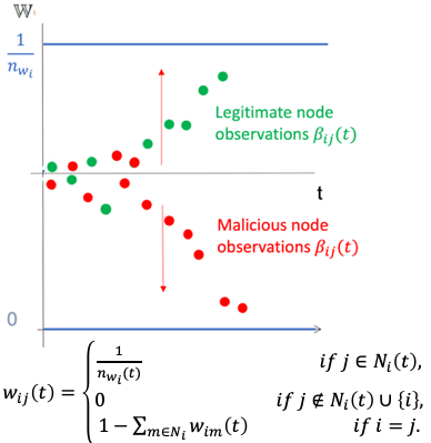
Intuitively, following the discussion after Definition II.2 of , the will tend towards positive values for legitimate agent transmissions , and will tend towards negative values for malicious agent transmissions where .
We also define a time dependent trusted neighborhood for each agent as:
| (7) |
This is the set of neighbors that legitimate agent classifies as its legitimate neighbors at time . Denote
where can be thought of as a parameter limiting the maximum influence that the neighbors of agent are allowed to have on agent ’s update values (i.e. a value of approaching infinity would preclude neighbors from influencing agent ’s updated values). Using these quantities, we define the weight matrix by choosing its entries as follows: for every , ,
| (8) |
Note that the dependence of the weights on the trust observation history comes in through the choice of time-dependent trusted neighborhood (cf. Eqn. 7). Note also that the matrix is a (rectangular) row-stochastic, by construction. Furthermore, since are random, so are the quantities and the set of neighbors of agents that agent classifies as legitimate at time . Consequently, some entries of the matrix are also random, as seen from (8). We use the parameter later on, in our analysis of the dynamics in (2), to obtain an upper bound on the entries of the matrix .
We define convergence as follows:
Definition II.3 (Convergence of the consensus protocol).
We define consensus to be achieved if:
1) Limit values:
There exists, almost surely, a random variable such that
| (9) |
where , and is in the convex hull of the legitimate agent values , and its distribution depends on the starting time of the consensus algorithm. Further, almost surely, a limit exists for the legitimate agent values which is a random variable such that
| (10) |
Here, is in the convex hull of the legitimate and malicious agent values , and its deviation from the nominal consensus value (the case with no malicious agents) depends on the starting time of the consensus algorithm. See Def. II.3.2 below.
2) Deviation: There is a probabilistic upper bound on the asymptotic
distance between the legitimate agent values and a suitably defined weighted average of their initial values, i.e.,
| (11) | |||
where is a user-defined error probability, while is the Perron-Frobenius left-eigenvector of the matrix defined in (12) such that .
We next discuss the assumptions that we use in the sequel. For this, we let be the subgraph of the graph that is induced by the legitimate agents, where is given by . We use the following assumptions throughout the paper:
Assumption 1.
Suppose that the following hold:
1. [Sufficiently connected graph]
The subgraph induced by the legitimate agents is connected.
2. [Homogeneity of trust variables]
The expectation of the variables are constant for the case of malicious transmissions and legitimate transmissions, respectively, i.e., for some scalars with ,
3. [Independence of trust observations] The observations are independent for all and all pairs of agents and , with , . Moreover, for any and , the observation sequence is identically distributed.
Assumption 1.1 captures the general connectivity requirement in consensus networks with a fixed topology. The assumption on the homogeneity of trust variables (cf. Assumption 1.2) is made only for the ease of exposition. The assumption can be generalized to the heterogeneous case as discussed in Section V.
II-B Problem Definition
In the following we summarize the three main problems that we aim to address under the assumptions in Assumption 1:
Problem 1 (Convergence of the consensus protocol).
We aim to show that in the presence of an adversarial attack, consensus to a common limit value is attainable even when malicious agents comprise of the network connectivity if observations are available. We seek conditions on , and a definition of the weights that allow convergence.
Problem 2 (Bounded deviation for average consensus).
For the case of average consensus, we aim to find a bound on deviation from the average consensus value, that can be achieved with a probability at least , where the bound is given as a function of problem parameters (such as the number of legitimate and the number of malicious agents) and the characteristics of (such as bounds on its expected value ).
Problem 3 (Characterization of convergence rate ).
We aim to determine a finite convergence time for the correct classification of legitimate and malicious agents almost surely. Additionally, we aim to identify the rate of convergence as a function of the stochastic observations and other problem parameters that we characterize.
III Analysis
III-A Convergence of Consensus of Legitimate Agents Inputs
In this section, we analyze the state dynamics among the legitimate agents, that is governed by the weight matrix , as seen from (2). Recalling that , from the definition of the matrix (cf. (8)), we see that the matrix is a sub-stochastic matrix, since the sum of some rows may be strictly less than one. This section analyzes the convergence of the (backward) product , as . We prove the strong ergodicity of this product, and show that the limit matrix has strictly positive entries, i.e., .
Our goal here is to show convergence of the consensus system in Eq. (2) using the choice of weights from Eq. (8) that exploit the observations . Specifically, we aim to characterize the conditions on necessary to achieve consensus in the presence of malicious agents even when the number of malicious agents is arbitrarily high.
We will achieve this in three parts: first we show that for a sufficiently connected network (cf. Assumption 1.1) the weight matrix in Eq. (8) reaches its limit described in Eq. (12) in finite time almost surely and that this limit is a primitive matrix (cf. Lemma 1 and Proposition 1). Second we show that this in turn implies that the legitimate agents’ influence captured in Eq. (4) approaches a finite limit almost surely (cf. Proposition 2). By the same token, the malicious agents’ influence captured in Eq. (5) also approaches a finite limit almost surely (c.f. Proposition 3). Finally, putting these limits together we show that the values of the legitimate agents, , approach a finite limit, i.e. we achieve convergence.
In what follows we use the notion of a primitive matrix, which is provided next.
Definition III.1 (Primitive matrix).
A nonnegative square matrix is said to be a primitive matrix if there exists an integer such that .
Let us define a matrix with the entries given by: for every ,
| (12) |
For the matrix , we have the following result.
Lemma 1.
The matrix is primitive.
Proof:
The result follows directly by the definition of the matrix in (12) and the assumption that the graph is connected (cf. Assumption 1.1). ∎
Under Assumptions 1.2–1.3, we next provide a result for the random quantities defining the weight matrix .
Lemma 2.
Consider the random variables as defined in (6). Then, for every and every ,
Additionally, for every and every ,
Proof:
From Lemma 2 one can observe the following.
Corollary 1 (Bounds on Expectation of ).
For the choice , we must have that for all and , for all to have a decaying misclassification probabilities.
We provide some intuition about this corollary as it has significant implications for the characteristics of necessary for obtaining several important results. The condition that and be bounded away from zero in Corollary 1 intuitively means that there is information captured by the observations. The case of , is equivalent to saying that, in expectation, the observations will be the same regardless of the transmission being legitimate or malicious (the observations contain no useful information). Hereafter, we assume that and , which means that tends to be less than for malicious transmissions (has expectation value less than ) and tends to be greater than for legitimate transmissions (has expectation value greater than ).
Proposition 1.
There exists a finite time instant such that for all almost surely. Moreover, there exists a stochastic vector such that
In particular, for every almost surely.
Proof:
By Lemma 2 we have that for every and , ,
| (13) |
Additionally, for every and , ,
| (14) |
Note that we have and . Thus, by the Borel-Cantelli Lemma, the events and occur only finitely often almost surely. Therefore, there exists a (random) finite time such that for all almost surely.
Now, almost surely, we have
By Lemma 1, the matrix is primitive. Therefore, by the Perron-Frobenius Theorem (see [59]), there exists a stochastic column vector such that .
Consequently, almost surely we have
Since and the diagonal entries of the matrices are positive (by construction), it follows that implying that almost surely ∎
Our next results are aimed at proving that the legitimate agents’ values reach consensus almost surely. In particular, using the decomposition of the legitimate agent states (see (3)), we focus on the limiting behavior of , as defined in (4). We show that converges almost surely to a consensus value, as , as seen in the following proposition.
Proposition 2 (Convergence of legitimate agents’ values).
Consider the dynamics in (2). Let be the vector of initial values of legitimate agents, and define
| (15) |
Then, we have for every , almost surely.
Proof:
By Proposition 1, there exists a finite time instant such that for all almost surely, and for a stochastic vector . Hence, it follows that almost surely
| (16) |
By letting , we obtain that , almost surely. ∎
We next consider the limiting effect that malicious agents’ states have on the legitimate agents’ states. Specifically, in the state decomposition relation for the legitimate agents’ states (see (3)), we focus on the limiting behavior of defined in (5), as . We show that converges to a consensus almost surely given our choice of weight matrices, as seen in the following proposition.
Proposition 3.
Consider the vector defined by
| (17) |
Then, the entries of this vector are all the same almost surely, i.e., almost surely for every .
Proof:
By Proposition 1, there exists a finite time instant such that almost surely,
| (18) |
This implies that for all almost surely. Therefore,
| (19) |
Now, for the product , we have that almost surely
where the second relation follows from (18).
By Proposition 1, we also have for a stochastic vector , such that . Hence, almost surely,
for some finite , implying that all the coordinates of the vector are identical almost surely. ∎
Corollary 2.
There exists, almost surely, a random variable such that
| (20) |
where is in the convex hull of the legitimate agents’ initial values , , and its distribution depends on the starting time of the consensus algorithm in (2). Furthermore, almost surely, there exists a random variable such that
| (21) |
where is in the convex hull of the initial values , of the legitimate and malicious agents, and its distribution depends on the starting time of the consensus algorithm.
Proof:
We note that, in the view of the fact that the legitimate agents start consensus protocol at time , we have that the random variable is in the convex hull of the initial values of legitimate agents. The random variable is in the convex hull of and the values , since the malicious agents may have deviated from their initial values at time .
We are now ready to state our main convergence result.
Theorem 1 (Convergence of Resilient Consensus).
Consider the consensus system described by the dynamics in Eq. (2) with an arbitrary start time of and weights as described by Eq. (8). Given that 1) is a sufficiently connected network and that 2) bounds on the expected values of the observations (see Defn. II.2) satisfy for all and for all , the consensus algorithm converges almost surely, i.e.,
almost surely, independently of the number of malicious agents in the network. The value is in the convex hull of the initial values of both the legitimate and malicious agents.
Proof:
Note that this result asserts convergence in the presence of an arbitrary number of malicious nodes and characterizes necessary conditions on the observations to attain this convergence. However, the distance of the limit value to the nominal average consensus value in the ideal case (when the malicious agents are known at the start time) has not been discussed. The characterization of this distance is the subject of the following section.
III-B Deviation from Nominal Consensus Value
In this section we characterize the deviation from the nominal consensus value under our consensus model in the presence of a malicious attack. The nominal consensus value is the consensus value over the graph of legitimate agents in the case of no malicious agents in the network. More specifically, by Proposition 1 we know that there exists a finite time instant such that for all almost surely, where is given in (12). The nominal consensus value corresponds to consensus that would have been reached among the legitimate agents if the dynamics in (2) were governed by instead of . Hence, in view of Proposition 1, the nominal consensus value over the graph of legitimate agents is .
In what follows we investigate the deviation of the consensus value reached by the legitimate agents (as predicted by Theorem 1) from the nominal value . The user-defined start time , for running the consensus dynamics in Eq. (2), plays a major role in determining the amount of the resulting deviation due to the malicious agents’ inputs to the system. Intuitively, the longer values are observed for all pairs before starting the consensus, the probability of making a misclassification error (classifying a legitimate agent as malicious and vice versa) decays exponentially.
Our approach in this section is to show that for larger values of , the probability of our weight matrix not having reached its limit value decays exponentially (see Lemma 3). The implication of this manifests itself as a smaller overall deviation. Specifically, deviation of the convergence limit (cf. Theorem 1) from the nominal average consensus value can be bounded by the deviation introduced by legitimate agents being misclassified as malicious and by malicious agents being misclassified as legitimate. Propositions 4 and 5 proven in this section provide definitive bounds for these deviations with probability which is characterized as a function of .
We begin by showing that the probability of the weights from Eq. (8) not taking their ideal form decays exponentially with .
Lemma 3.
For every
Proof:
Next, we consider the deviation contributed by misclassifying legitimate agents as malicious at some times and, thus, discarding their values. In the sequel, we use the bound of Lemma 3 to define a quantity for an error tolerance . Specifically, given , we define
| (24) |
where is a finite upper bound on the absolute input value.
In what follows, we make use of the following lemma.
Lemma 4.
Let be two row-substochastic matrices, and let be such that and for all . Then , for all , where denote the matrix with entries .
Proof:
Let coordinate index be arbitrary, . First, we prove that . By the triangle inequality, we obtain
Since and we have that
Therefore, it follows that
where the last inequality is obtained by using the triangle inequality and the fact that the matrices and have nonnegative entries. Since both and are stochastic matrices, we further have that . From the preceding two relations, it follows that . ∎
Denote by the deviation suffered by legitimate agent that is caused by its incorrect classification of the legitimate agents, i.e., for all ,
| (25) |
Proposition 4.
Proof:
Let be a random variable equal to if for all , and equal to , otherwise. In view of the evolution of as given in (4), we have
Define
Then,
| (26) |
where follows since is a row-stochastic matrix. Further, since , it follows that
where for a matrix , we use to denote the matrix with entries . Therefore,
Let and note that is a stochastic matrix with (see (12)). Additionally, for every , the matrix is substochastic with for every . Therefore, by Lemma 4 we have
Define
Then, we have for all and , thus implying that
By Proposition 1, for , we have almost surely, implying that almost surely converges as . By Markov’s inequality it follows that
By definition, for every we have that , therefore, for every . Hence, by the Monotone Convergence Theorem (see [60]), it follows that
Since , it further follows that
where the last inequality follows from Lemma 3 and the definition of in (III-B). ∎
Now we consider the deviation contributed by malicious agents that are misclassified as legitimate. We denote by , , the worst case effect on legitimate agent due to its incorrect malicious agents’ classification (labeling an untrustworthy agent as trustworthy) at some time . Specifically, let and define
| (27) |
for all . We note that these quantities are nonnegative, since the matrices and are nonnegative for all . Looking at the malicious agents’ influence vector defined in (5), we see that
Our next result provides a probabilistic bound on the maximal influence of malicious agents inputs on the legitimate agents’ values. To do so, given , we define
| (28) |
where .
Proposition 5.
Proof:
First, observe that
It follows by Markov’s inequality and the linearity of the expectation operator that
In view the definition of , to complete the proof, it suffices to show that
| (30) |
The rest of the proof deals with establishing relation (30). By the definition of , in (27), we have that
where the inequality is obtained by using the fact that is a row-substochastic matrix. Moreover, we have that (see (8)), implying that
| (31) | ||||
| (32) |
Hence,
| (33) |
By the definition of in (31), the sequence is a nonnegative non-decreasing sequence with . Therefore, by the Monotone Convergence Theorem [60],
| (34) | ||||
| (35) |
We further have that
Since , we obtain that
where the last inequality follows by Lemma 2. Hence,
| (36) | ||||
| (37) | ||||
| (38) |
By combining estimates in (33)–(36), the desired relation in (30) follows. ∎
We are now ready to prove our main deviation result which states that the maximum deviation of the converged consensus value following the dynamics in Eq. (2) with the weights described in Eq. (8) can be bounded by a finite value that we characterize.
Theorem 2 (Deviation from Nominal Average Consensus).
Consider the consensus system described by the dynamics in Eq. (2) with an arbitrary start time of and weights as described by Eq. (8). Given that 1) is a sufficiently connected network and that 2) bounds on the expected values of the observations (see Defn. II.2) satisfy for all , and for all , for a given error probability , we have the following result
where
| (39) |
with and respectively given by
and
Proof:
First, note that by the triangle inequality
Since is a primitive stochastic matrix, by the Perron-Frobenius Theorem it follows that
Thus,
Now, since , by the triangle inequality we have
It follows by the definition of in (39) and the union bound that
Since and , it follows that
Finally, by Proposition 4 we have
while, similarly, by Proposition 5 we have
∎
Thus, we have solved Problem 2 by showing that beyond achieving convergence of consensus in the face of a malicious attack, the deviation of the converged value from the nominal average consensus value (in the case of no malicious agents) can be characterized as a function of user-defined parameters and failure probability . In the next section we characterize convergence rate of our consensus protocol.
III-C Convergence Rate of Resilient Consensus
In this section we discuss convergence rate for the consensus protocol in Eq. (2) using the weights as defined in Eq. (8). Let
We start by presenting a useful lemma showing a contraction property for a consensus step using a primitive matrix that we will later employ.
Lemma 5.
Assume that if and only if for every (i.e., bidirectional links between legitimate agents). Let denote the second largest eigenvalue modulus222The second largest absolute value of the eigenvalues. of and let be the stochastic Perron vector satisfying . Then,
Proof:
It can be seen that the Perron vector has entries for all , implying that is reversible Markov chain. Thus, the result follows from the convergence rate of reversible Markov chains (see [61]). ∎
We are now ready to prove our convergence rate results. Namely, we show that the rate of convergence of legitimate agents to their limit value is governed by the second largest eigenvalue modulus of the ideal weight matrix with a probability that approaches 1 exponentially, as increases.
Theorem 3 (Convergence Rate of Resilient Consensus).
Consider the consensus system described by the dynamics in Eq. (2) with an arbitrary start time of and weights as described by Eq. (8). Assume that 1) is a sufficiently connected network and that 2) bounds on the expected values of the observations (see Defn. II.2) satisfy for all , for all and for all , for all . Let denote the second largest eigenvalue modulus of and let be the stochastic Perron vector satisfying . Additionally, let and assume that if and only if for every . For every , if we start the consensus protocol from time , then for every and , we have
| (40) |
with a probability greater than
| (41) |
Proof:
Recall that almost surely. Since , it follows by the triangle inequality that
Now, assume that for all , and . Then, by the Perron-Frobenius Theorem and the definition of ,
Additionally,
Finally, following the proof of Lemma 3, we can lower bound the probability of the event that and for all by (41). ∎
As an immediate consequence of Theorem 3, we have the following result.
Corollary 3.
Under the conditions of Theorem 3, for every and we have
Note that choosing yields the bound
where .
III-D Tightening the probabilistic bounds
Up until this point we have placed a mild information assumption on the (this was a consequence of Lemma 2); namely that the expected values of the are strictly bounded away from 1/2 as required in Corollary 1. In words this means that there is some information contained in the observations such that in expectation these values are closer to 0 for transmissions from legitimate agents and closer to 1 for transmissions from malicious agents. An expected value of equal to 1/2 would be the case of no information. Thus this is the mildest assumption possible for the and is the key to the decaying probabilities from Lemma 2 that underpin the majority of our presented results in this paper. However, if it is possible to obtain more information on the , for example knowing a bound on its variance, then the probabilistic bounds can be made tighter and the resulting performance guarantees such as bounds on the deviation can be made stronger. This observation is substantiated with analysis in the current section.
Lemma 2 lays the foundation for deriving the convergence of consensus of legitimate agents presented in Theorem 1, the deviation probabilistic bound presented in Theorem 2 and and the probabilistic upper bound on the convergence rate presented in Theorem 3. Lemma 2 considers a large family of probability measures for the random variables where only the expectation of the variables are fixed to known values. While the bounds derived in Lemma 2 decay exponentially over time, they are somewhat loose when higher moments of the random variables are known. In the special case when the random variables belong to a family of probability measures of known variance values, we can use the concentration inequalities that consider both the first and second moments, instead of the Chernoff-Hoeffding concentration inequality used in the proof of Lemma 2. Prominent examples of such inequalities are the Berstein inequality, Bennet’s inequality and the improved Bennet’s inequality, providing more refined results than the Chernoff-Hoeffding inequality, are included here for completeness.
Theorem 4 (Berstein inequality).
Assume that are independent random variables and , and almost surely. Then,
Theorem 5 (Bennet’s inequality [62]).
Assume that are independent random variables and , and almost surely. Then, for any ,
where and .
Theorem 6 (Improved Bennet’s inequality [63]).
Assume that are independent random variables and , and almost surely. Additionally, let
and , where is the Lambert function. Let , then for any ,
As stated in [64], Bennet’s inequality yields strictly tighter approximation than Bernstein’s inequality. Bennet’s inequality, in turn, is tightened by the improved Bennet’s inequality. For this reason, we present in Lemma 6 refined concentration inequalities that improve those presented in Lemma 2 using the improved Bennet’s inequality. Recall Assumption 1.2 and Assumption 1.3, and additionally assume that
and that
Applying these tighter concentration inequalities to the history of observations , we can obtain a faster exponential rate result for the decay of misclassification probabilities (misclassifying a legitimate agent as malicious or a malicious agent as legitimate) than that of Lemma 2, as seen in the following.
Lemma 6.
Consider the random variables defined in Equation (6) for every legitimate node and every neighbor . Then, for every and every ,
where for , , and
with being the Lambert function, and
Moreover, for every and every ,
where for , and , with scalars and given by
Proof:
Let , , and note that the given probabilistic bound holds trivially when , so assume that and define
Since , for the random variable we have and . Since , it follows that implying that . Also, since and it follows that . Thus, . Using the definition of in (6), we have
We now invoke Theorem 6 for the sequence of random variables , with , and , which yields the desired relation. Note that the condition in Theorem 6 is satisfied in our case here, since with and .
Consider now the case , . If , then the result holds trivially. Thus, assume that , and consider
Since , we have that and . Additionally, since , we can see (similar to the preceding case) that . Hence,
Recall that , so we can invoke Theorem 6 for the sequence of random variables , with , , and . Since and , it follows that . Thus, in our case here, the condition in Theorem 6 reduces to which holds since . ∎
Therefore, in the case that additional information on the observations is available, in particular that a bound on the variance of the is known, then the results of Lemma 2 can be replaced with Lemma 6, resulting in tighter deviation and convergence rate results when applied to Theorems 2 and 3. This shows the generality of our framework and the potential to improve our derived performance guarantees as more information on the observations becomes available. Similarly, Lemma 6 can be extended to the case where varies over time and is link dependent.
IV Numerical Results
In this section we evaluate the performance of the proposed scheme in this work using Monte Carlo simulations. We aim at investigating the effects, on several performance metrics, of the following system parameters: the number of malicious agents, the starting time of the data passing stage and the variance of the random variables . Performance metrics that we study include deviation from the true consensus value and the convergence rate. We evaluate a system setup with legitimate agents, and with . We consider the following values for the starting time : 0, 25, 50, 100, 150. The adjacency matrix of the subgraph of links among legitimate agents is
| (42) |
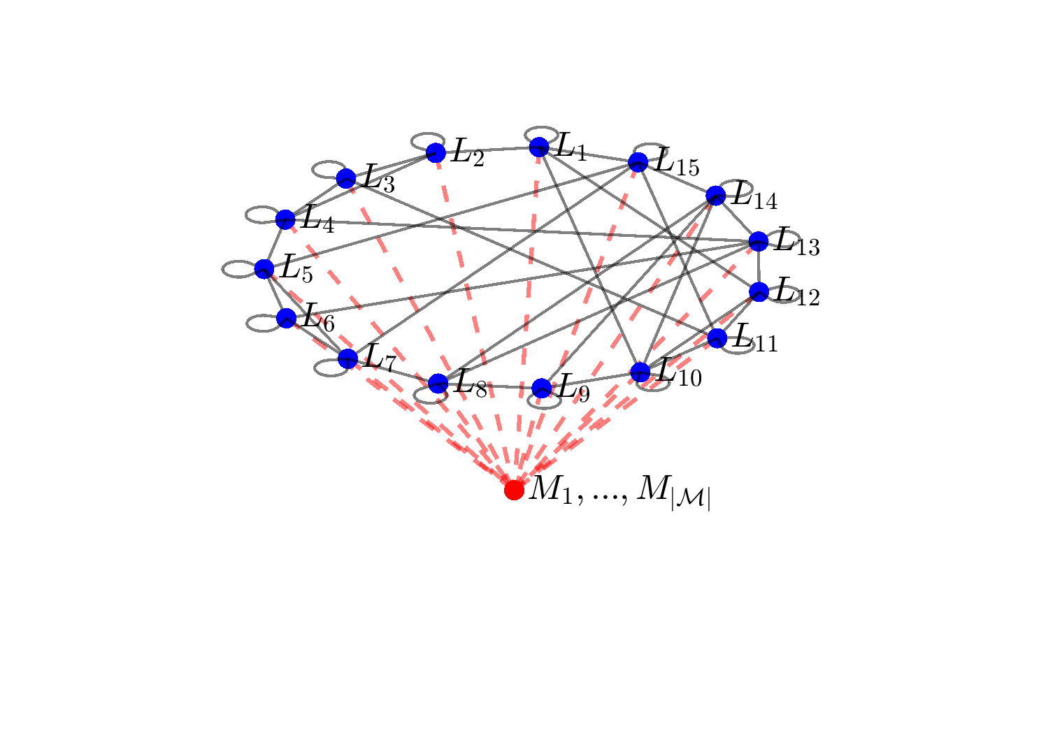
and we assume that every malicious agent is connected to all the legitimate agents in the system which is the worst-case scenario. We depict the topology corresponding to the connectivity graph in Figure 4; since every malicious agent is connected to all legitimate agents we depict the malicious agents in Figure 4 by a single node.
The vector of initial values of legitimate agents is
where denotes the transpose operator, and we use as the upper bound for the agents’ initial values. Additionally, for every legitimate agent , we have if , and if . The random variable is uniformly distributed on the interval . We consider the following three values for : , for which the standard deviation values are , respectively. Note that the larger the , the larger the variance of about its mean value. We consider the following input scenarios presented in Figures 5 and 6. Both attacks assume that the malicious agents are allowed to communicate and coordinate attacks.
Maximal deviation malicious input
To measure the maximal possible deviation from true consensus value we consider the case were the malicious agents inputs are the furthest from the true consensus value. That is, if the true consensus value is positive than the malicious input is , and if the true consensus value is negative than the malicious input is . In our scenario, all the malicious agents choose the maximum possible input . Figures 5 and 7 measure the effect of the malicious agent inputs that lead to the maximum deviation from the true consensus value. Figure 5 depicts agent values over time when running consensus according to the protocol from Equation (1) and the weights defined by Equation (8). Specifically, Figure 5 depicts the value of the agent with the maximal deviation from the true consensus value for a single system realization with maximum deviation malicious input. Additionally, Figure 7 depicts the absolute value of the maximum deviation from the true consensus value averaged over 500 system realizations. Figures 5 and 7 additionally show the differences in converged values and deviation respectively for different consensus start times .
The maximum deviation malicious input leads to an upper bound to all possible malicious attacks, and depicts a worst case scenario in terms of deviation from true consensus value. However, though this attack is useful to analyze the worst case effect of malicious inputs it is easy to detect using outlier rejection methods for example [8]. For this reason, we consider the following additional attack scenario that is harder to detect.
Drift malicious input
Figure 6 and 8 measure the effect of a less transparent malicious agents’ attack where every malicious agent adds a drift term to the average legitimate agent values. More specifically, let be the average value at time of the legitimate agents that are neighbors of the malicious agent . Denote . Then, at time , the malicious agent chooses its state value according to the following rule:
where is chosen randomly from the set and for every
. Thus malicious agent inputs are time varying and strategically close to legitimate agent values to avoid easy detection in this case. Additionally, if then is generated randomly and uniformly from the interval . Similarly if then is generated randomly and uniformly from the interval . We note that since in our scenario every malicious agents is a neighbor of all the legitimate agents, for all . Figure 6 depicts the value of the agent with the maximal deviation from the true consensus value for a single system realization with drift malicious input. Additionally, Figure 8 depicts the resulting absolute value of the maximum deviation from the true consensus value for a drift malicious input averaged over 500 system realizations.
Figures 5 and 6 depict a single realization of the agent value with the maximal deviation from true consensus value for a system with 15 malicious agents and . Figure 5 depicts the agent value with the maximal deviation from true consensus value for the maximal deviation malicious inputs where Figure 6 depicts the agent value with the maximal deviation from true consensus value for the drift malicious inputs.
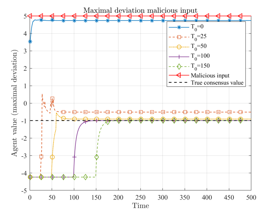
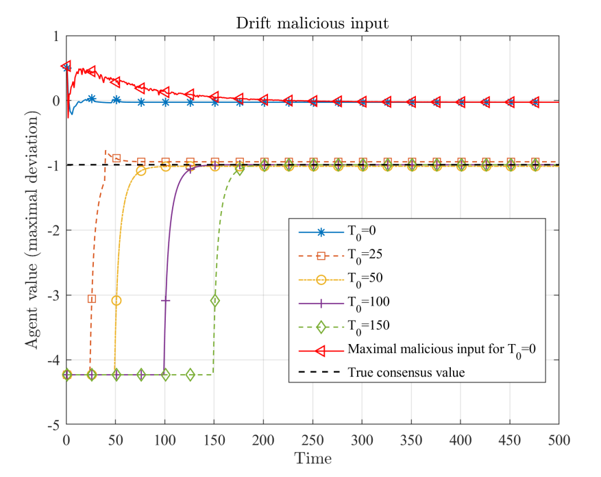
In addition to Figures 5 and 6 that depict the legitimate agent values for a single system realization we depict in Figures 7 and 8 the average deviation of the legitimate agent values from true consensus value. The average deviation is calculated using 500 system realizations. Figures 7 and 8 show that the deviation from true consensus value grows both as grows and as the number of malicious agents grows. In each figure we label the plot by (R#,C#) where R# denotes the row number and represents the increase in the number of malicious agents, and C# denotes the column number and represents the growth of . Figures 7 and 8 show the significance of introducing the variable that sets the starting time of the data passing between agents. The figures indicate that increasing can significantly reduce the deviation from true consensus value. Figures 7 and 8 also show that our scheme can combat an attack of a large number of malicious agents, even when , that is, there is twice the number of malicious agents than legitimate agents in the system. This is a significant improvement over classical results that depend on the network connectivity [1, 6, 5]. Using the upper bound on the network connectivity we can conclude that classical results will fail to detect all the malicious agents when their number is larger than the number of legitimate agents; in this case the undetected malicious agents can control the data values of the legitimate agents. More specifically, we can see from the choice of adjacency matrix (42) that for our setup, the network connectivity is at most and thus classical results can tolerate less than malicious agents. Since there are malicious agents, the consensus algorithm can fail and be controlled by the malicious agents. Furthermore, for the connectivity graph that we consider in the numerical results, the maximal number of malicious agents leading to a graph connectivity guaranteeing their detection and preventing them from controlling the network is , since we must fulfill the condition that . Finally, our numerical results show that there exists a finite time such that the probability to classify all the user in the network correctly for every is sufficiently high. We can see from Figures 7 and 8 that the minimal value of that yields a negligible deviation from true consensus value depends on probability of miss-classifying users, i.e., classifying a legitimate agent as malicious and vice-versa. This probability is increased, for example, as the number of malicious agents grows and as the variance of grows. Figures 7 and 8 show that as we increase the number of malicious agents and the deviation that governs the variance of we should increase to limit the effect of the malicious agents on the consensus value. Additionally, Figures 7 and 8 show that the for the deviation from true consensus value for all considered scenarios is negligible. Finally, for the deviation from true consensus value is sufficiently small and the effect of malicious agents is limited even for .
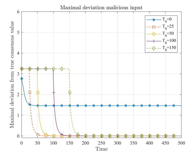
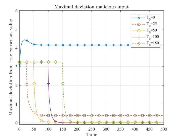
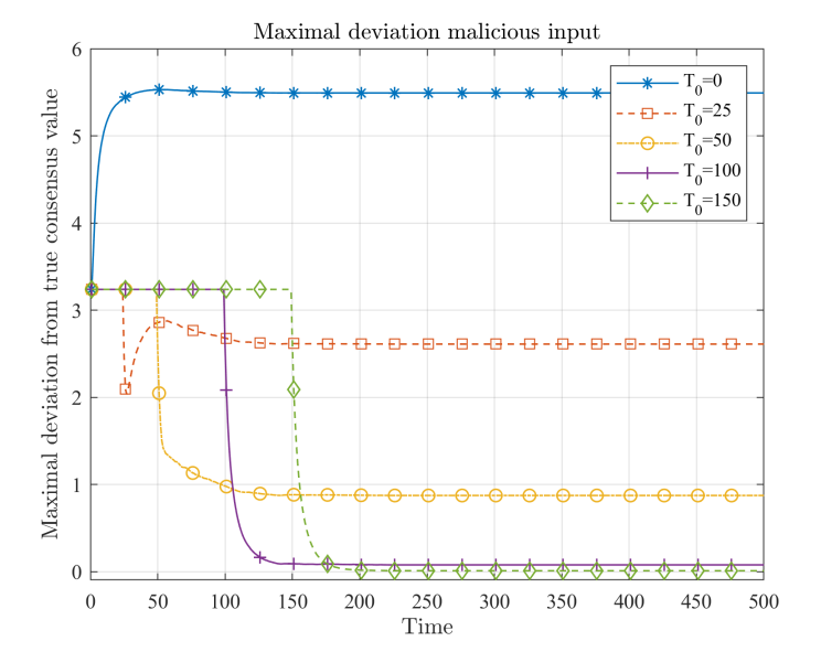
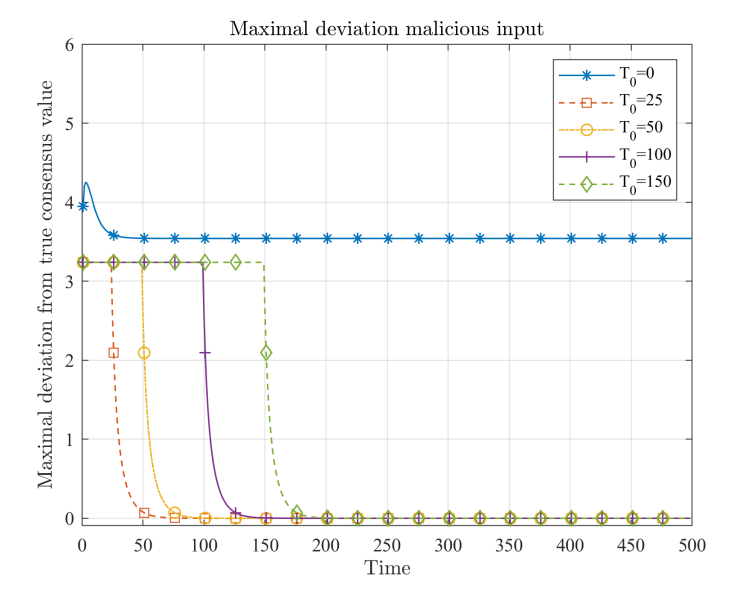
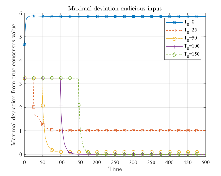
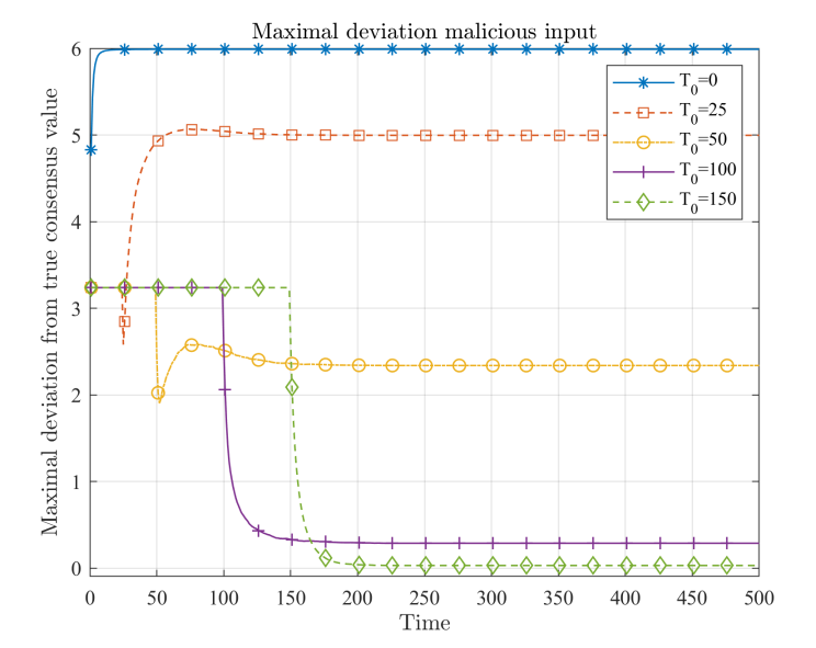
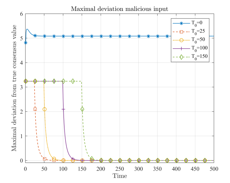
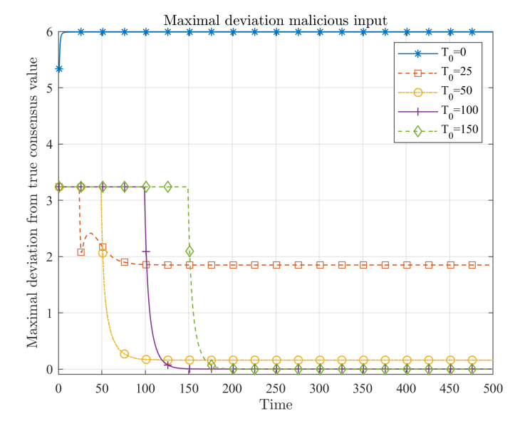
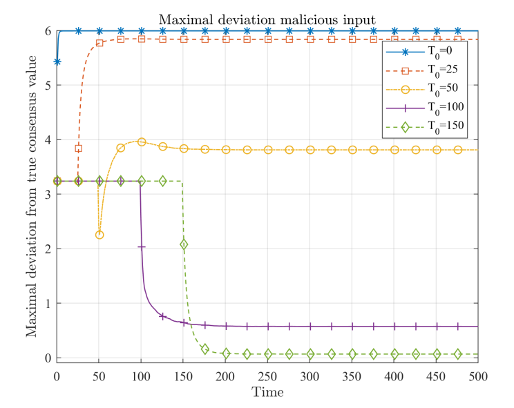
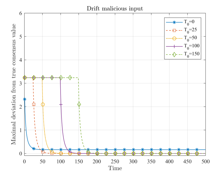
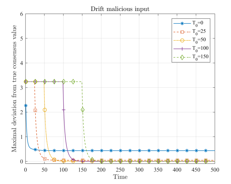
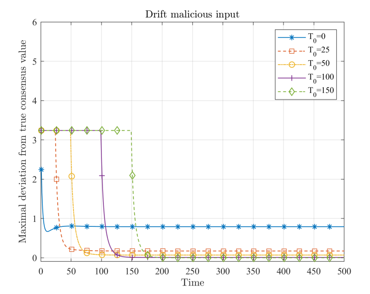
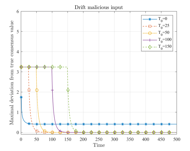
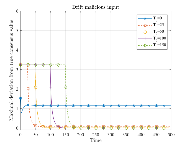
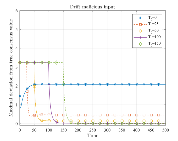
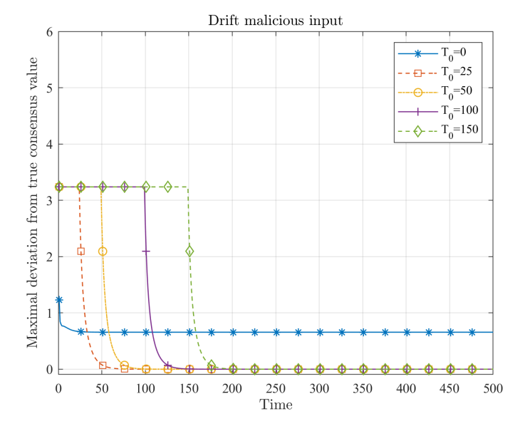
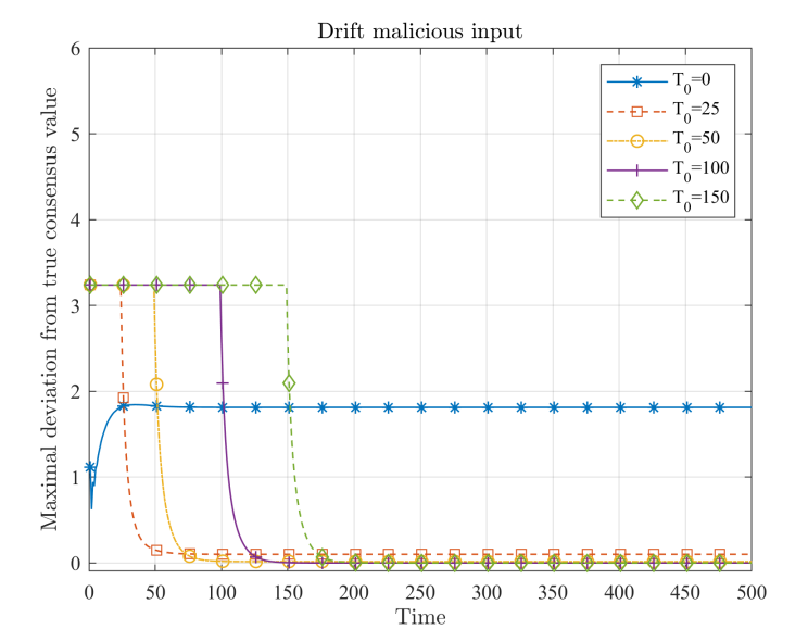
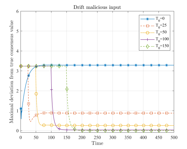
Figure 7 shows that as becomes larger (and therefore also the variance), the effect of malicious agents on deviation gets worse. However, even in this case increasing can recover the nominal consensus value with deviation approaching zero. The exact relationship between the deviation and is given by Theorem 2.
In the case of a time varying malicious agent input as with the drift malicious input model described in part (b) of this section, nominal average consensus can also be recovered by making larger, as depicted in Figure 8. This is true even with variable variance on the values.
V Discussion
In this section we discuss the significance of some of our characterizations on the trust observations and some of our assumptions. We also discuss directions for future work. Firstly, the results of this paper assume a fixed network topology. However, we believe that it is possible to relax Assumption 1.1 to include the case where the graph over legitimate agents is not always connected. In such a case Assumption 1.1 can be replaced with the assumption that the topology of the legitimate agents is B-connected.333See definition in [29]. We believe that the convergence results from [65, Proposition 1] can be adapted to this case along the same vein as in Theorem 3. We now comment on independence of the values which is an important assumption for the application of concentration inequalities such as those used in our derivations. Conditioned on being legitimate or spoofed, computation of the values will be subject to noise experienced over the wireless channel. This is widely assumed to be Gaussian white noise [48] that is independent with respect to time. In addition, for uniform scattering environments signal paths decorrelate spatially [47]. However, it is possible that since the terms also have a dependence on the environment, in the uncommon case that the environment and all robots stay perfectly static, then complete independence may no longer hold. Relaxing these assumptions may also be an interesting avenue for future work. Finally we discuss a few interesting observations about the trust values . Our results show that the more informed our values are, the tighter the performance guarantees achievable become (cf. Lemma 6). This also opens a future avenue of investigation of finding observations from physical channels in multi-agent systems which can be characterized as fully as possible. The theory in this paper provides the mathematical framework for understanding which characteristics of are most critical for attaining performance guarantees that are important for multi-agent coordination. We hope that this can guide continued investigation into trust-based resilience, particularly for cyberphysical systems where additional information on inter-agent trust can be attained.
VI Conclusion
This paper presents a unified mathematical theory to treat distributed multi-agent consensus in the presence of malicious agents when stochastic values of trust between agents are available. Under this model, we present three new performance guarantees for consensus systems in the presence of malicious agents: 1) convergence of consensus is possible with probability 1 even when the number of malicious agents is far larger than 1/2 of the network connectivity– in contrast to classical results in resilience, 2) the deviation of the converged value from average consensus can be bounded and further, can be driven arbitrarily close to zero by using our derived edge weights and by allowing an observation time of trust values over the network, and 3) convergence to the correct classification of agents can be attained in finite time with probability 1 with an exponential rate that we derive. Additionally, we show that our performance guarantees can be made stronger if more information on the trust observations, such as bounds on their variance, is available. Taken together, these results point to the inherent value of quantifying and exploiting trust between agents for consensus. We believe that the mathematical formulations and framework of this paper hold promise for achieving a new generation of resilient multi-agent systems.
References
- [1] D. Dolev, “The byzantine generals strike again,” Journal of Algorithms, vol. 3, no. 1, pp. 14 – 30, 1982. [Online]. Available: http://www.sciencedirect.com/science/article/pii/0196677482900049
- [2] M. J. Fischer, N. A. Lynch, and M. S. Paterson, “Impossibility of distributed consensus with one faulty process,” J. ACM, vol. 32, no. 2, p. 374–382, Apr. 1985.
- [3] L. Lamport, “Paxos made simple,” ACM SIGACT News 32, pp. 18–25, Dec 2001.
- [4] R. D. Prisco, B. Lampson, and N. Lynch, “Revisiting the paxos algorithm,” Theoretical Computer Science, vol. 243, no. 1, pp. 35 – 91, 2000.
- [5] S. Sundaram and C. N. Hadjicostis, “Distributed function calculation via linear iterative strategies in the presence of malicious agents,” IEEE Transactions on Automatic Control, vol. 56, no. 7, pp. 1495–1508, 2011.
- [6] F. Pasqualetti, A. Bicchi, and F. Bullo, “Consensus computation in unreliable networks: A system theoretic approach,” IEEE Transactions on Automatic Control, vol. 57, no. 1, pp. 90–104, Jan 2012.
- [7] F. Higgins et al., “Threats to the swarm: Security considerations for swarm robotics,” International Journal on Advances in Security, 2009.
- [8] H. J. LeBlanc, H. Zhang, X. Koutsoukos, and S. Sundaram, “Resilient asymptotic consensus in robust networks,” IEEE Journal on Selected Areas in Communications, vol. 31, no. 4, pp. 766–781, April 2013.
- [9] S. K. Khaitan and J. D. McCalley, “Design techniques and applications of cyberphysical systems: A survey,” IEEE Systems Journal, vol. 9, no. 2, pp. 350–365, 2015.
- [10] F. Pasqualetti, F. Dorfler, and F. Bullo, “Control-theoretic methods for cyberphysical security: Geometric principles for optimal cross-layer resilient control systems,” IEEE Control Systems Magazine, vol. 35, no. 1, pp. 110–127, 2015.
- [11] S. Pequito, F. Khorrami, P. Krishnamurthy, and G. J. Pappas, “Analysis and design of actuation–sensing–communication interconnection structures toward secured/resilient lti closed-loop systems,” IEEE Transactions on Control of Network Systems, vol. 6, no. 2, pp. 667–678, 2019.
- [12] J. Giraldo, D. Urbina, A. Cardenas, J. Valente, M. Faisal, J. Ruths, N. O. Tippenhauer, H. Sandberg, and R. Candell, “A survey of physics-based attack detection in cyber-physical systems,” ACM Comput. Surv., vol. 51, no. 4, Jul. 2018.
- [13] A. Tsiamis, K. Gatsis, and G. J. Pappas, “State-secrecy codes for networked linear systems,” IEEE Transactions on Automatic Control, vol. 65, no. 5, pp. 2001–2015, 2020.
- [14] Y. Mo, S. Weerakkody, and B. Sinopoli, “Physical authentication of control systems: Designing watermarked control inputs to detect counterfeit sensor outputs,” IEEE Control Systems Magazine, vol. 35, no. 1, pp. 93–109, 2015.
- [15] F. Adib, Z. Kabelac, D. Katabi, and R. C. Miller, “3d tracking via body radio reflections,” in 11th USENIX Symposium on Networked Systems Design and Implementation (NSDI 14). Seattle, WA: USENIX Association, Apr. 2014, pp. 317–329.
- [16] J. Xiong and K. Jamieson, “Arraytrack: A fine-grained indoor location system,” in Presented as part of the 10th USENIX Symposium on Networked Systems Design and Implementation (NSDI 13). Lombard, IL: USENIX, 2013, pp. 71–84.
- [17] M. Kotaru, K. Joshi, D. Bharadia, and S. Katti, “Spotfi: Decimeter level localization using wifi,” SIGCOMM Comput. Commun. Rev., vol. 45, no. 4, p. 269–282, Aug. 2015. [Online]. Available: https://doi.org/10.1145/2829988.2787487
- [18] J. Wang, F. Adib, R. Knepper, D. Katabi, and D. Rus, “Rf-compass: Robot object manipulation using rfids,” ser. MobiCom, 2013.
- [19] J. Xiong and K. Jamieson, “Securearray: Improving wifi security with fine-grained physical-layer information,” in Proceedings of the 19th Annual International Conference on Mobile Computing and Networking, ser. MobiCom, 2013.
- [20] S. Gil, S. Kumar, M. Mazumder, D. Katabi, and D. Rus, “Guaranteeing spoof-resilient multi-robot networks,” AuRo, p. 1383–1400, 2017.
- [21] J. Fax and R. Murray, “Information flow and cooperative control of vehicle formations,” Automatic Control, IEEE Transactions on, 2004.
- [22] N. A. Lynch, Distributed Algorithms. San Francisco, CA, USA: Morgan Kaufmann Publishers Inc., 1996.
- [23] M. M. Zavlanos, M. B. Egerstedt, and G. J. Pappas, “Graph-theoretic connectivity control of mobile robot networks,” Proceedings of the IEEE, vol. 99, no. 9, pp. 1525–1540, 2011.
- [24] D. P. Spanos and R. M. Murray, “Motion planning with wireless network constraints,” in ACC, 2005.
- [25] A. Nedić, A. Ozdaglar, and P. A. Parrilo, “Constrained consensus and optimization in multi-agent networks,” IEEE Transactions on Automatic Control, vol. 55, no. 4, pp. 922–938, 2010.
- [26] A. Nedić, A. Olshevsky, and W. Shi, “Achieving geometric convergence for distributed optimization over time-varying graphs,” SIAM Journal on Optimization, vol. 27, no. 4, pp. 2597–2633, 2017.
- [27] J. M. Hendrickx and J. N. Tsitsiklis, “Convergence of type-symmetric and cut-balanced consensus seeking systems,” IEEE Transactions on Automatic Control, vol. 58, no. 1, pp. 214–218, 2013.
- [28] R. Olfati-Saber and R. M. Murray, “Consensus problems in networks of agents with switching topology and time-delays,” IEEE Transactions on Automatic Control, 2004.
- [29] A. Nedić, A. Olshevsky, and M. G. Rabbat, “Network topology and communication-computation tradeoffs in decentralized optimization,” Proceedings of the IEEE, vol. 106, no. 5, pp. 953–976, 2018.
- [30] L. Xiao and S. Boyd, “Fast linear iterations for distributed averaging,” Systems and Control Letters, 2004.
- [31] A. Nedić, “Convergence rate of distributed averaging dynamics and optimization in networks,” Foundations and Trends® in Systems and Control, vol. 2, no. 1, pp. 1–100, 2015.
- [32] A. Olshevsky and J. N. Tsitsiklis, “Convergence speed in distributed consensus and averaging,” SIAM Rev., vol. 53, no. 4, p. 747–772, Nov. 2011.
- [33] X. Liu and J. S. Baras, “Using trust in distributed consensus with adversaries in sensor and other networks,” in 17th International Conference on Information Fusion (FUSION), 2014, pp. 1–7.
- [34] W. Tong, X. Dong, and J. Zheng, “Trust-pbft: A peertrust-based practical byzantine consensus algorithm,” in 2019 International Conference on Networking and Network Applications (NaNA), 2019, pp. 344–349.
- [35] I. Sargeant and A. Tomlinson, “Modelling malicious entities in a robotic swarm,” in DASC, 2013.
- [36] F. Higgins, A. Tomlinson, and K. M. Martin, “Threats to the swarm: Security considerations for swarm robotics,” International Journal on Advances in Security, vol. 2, pp. 288–297, 2009.
- [37] F. Higgins, A. Tomlinson, and K. M. Martin, “Survey on security challenges for swarm robotics,” in Fifth International Conference on Autonomic and Autonomous Systems (ICAS) 2009, 2009.
- [38] A. A. Cárdenas, T. Roosta, G. Taban, and S. Sastry, Cyber Security: Basic Defenses and Attack Trends, 2008, pp. 73–101.
- [39] A. A. Cárdenas et al., “Attacks against process control systems: Risk assessment, detection, and response,” ser. ASIACCS ’11, 2011.
- [40] J. Yang, Y. Chen, W. Trappe, and J. Cheng, “Detection and localization of multiple spoofing attackers in wireless networks,” IEEE Transactions on Parallel and Distributed Systems, vol. 24, no. 1, pp. 44–58, 2013.
- [41] H. Sandberg, S. Amin, and K. H. Johansson, “Cyberphysical security in networked control systems: An introduction to the issue,” IEEE Control Systems Magazine, vol. 35, no. 1, pp. 20–23, 2015.
- [42] S. Amin, A. A. Cárdenas, and S. S. Sastry, “Safe and secure networked control systems under denial-of-service attacks,” HSCC, pp. 31–45, 2009.
- [43] A. A. Cardenas, S. Amin, and S. Sastry, “Secure control: Towards survivable cyber-physical systems,” in 2008 The 28th International Conference on Distributed Computing Systems Workshops, 2008, pp. 495–500.
- [44] K. Saulnier, D. Saldaña, A. Prorok, G. J. Pappas, and V. Kumar, “Resilient flocking for mobile robot teams,” IEEE Robotics and Automation Letters, vol. 2, no. 2, pp. 1039–1046, April 2017.
- [45] M. Krotofil, J. Larsen, and D. Gollmann, “The process matters: Ensuring data veracity in cyber-physical systems,” in Proceedings of the 10th ACM Symposium on Information, Computer and Communications Security. New York, NY, USA: Association for Computing Machinery, 2015, p. 133–144.
- [46] J. Lin, S. Sedigh, and A. Miller, “A general framework for quantitative modeling of dependability in cyber-physical systems: A proposal for doctoral research,” in 2009 33rd Annual IEEE International Computer Software and Applications Conference, vol. 1, 2009, pp. 668–671.
- [47] A. Goldsmith, Wireless Communications. New York, NY, USA: Cambridge University Press, 2005.
- [48] D. Tse and P. Vishwanath, Fundamentals of Wireless Communications. Cambridge University Press, 2005.
- [49] S. Kumar, E. Hamed, D. Katabi, and L. Erran Li, “LTE radio analytics made easy and accessible,” in SIGCOMM, 2014.
- [50] S. Kumar et al., “Accurate indoor localization with zero start-up cost,” ser. MobiCom, 2014.
- [51] N. Jadhav, W. Wang, D. Zhang, O. Khatib, S. Kumar, and S. Gil, “WSR: A WiFi sensor for collaborative robotics,” in arXiv:2012.04174, 2020.
- [52] K. Zeng, K. Govindan, and P. Mohapatra, “Non-cryptographic authentication and identification in wireless networks [security and privacy in emerging wireless networks],” IEEE Wireless Communications, vol. 17, no. 5, pp. 56–62, 2010.
- [53] T. Wang and Y. Yang, “Analysis on perfect location spoofing attacks using beamforming,” in INFOCOM, 2013.
- [54] D. Moser, P. Leu, V. Lenders, A. Ranganathan, F. Ricciato, and S. Capkun, “Investigation of multi-device location spoofing attacks on air traffic control and possible countermeasures,” in Proceedings of the 22Nd Annual International Conference on Mobile Computing and Networking, ser. MobiCom ’16. New York, NY, USA: ACM, 2016, pp. 375–386.
- [55] S. Gil, S. Kumar, M. Mazumder, D. Katabi, and D. Rus, “Adaptive communication in multi-robot systems using directionality of signal strength,” IJRR, 2015.
- [56] S. Gil, C. Baykal, and D. Rus, “Resilient multi-agent consensus using wi-fi signals,” IEEE Control Systems Letters, vol. 3, no. 1, pp. 126–131, Jan 2019.
- [57] T. Wheeler, E. Bharathi, and S. Gil, “Switching topology for resilient consensus using wi-fi signals,” in 2019 International Conference on Robotics and Automation (ICRA), 2019, pp. 2018–2024.
- [58] D. P. Dubhashi and A. Panconesi, “Concentration of measure for the analysis of randomized algorithms.” Cambridge University Press, 2009.
- [59] S. U. Pillai, T. Suel, and Seunghun Cha, “The perron-frobenius theorem: some of its applications,” IEEE Signal Processing Magazine, vol. 22, no. 2, pp. 62–75, 2005.
- [60] R. Durrett, Probability: Theory and Examples, 4th ed. Cambridge University Press, 2010.
- [61] P. Brémaud, Gibbs Fields, Monte Carlo Simulation, and Queues. New York, USA: Springer-Verlag, 1999.
- [62] G. Bennett, “Probability inequalities for the sum of independent random variables,” Journal of the American Statistical Association, vol. 57, no. 297, pp. 33–45, 1962.
- [63] S. Zheng, “An improved bennett’s inequality,” Communications in Statistics - Theory and Methods, vol. 47, no. 17, pp. 4152–4159, 2018.
- [64] T. Jebara, “A refinement of Bennett’s inequality with applications to portfolio optimization,” in arXiv:1804.05454, 2018.
- [65] A. Nedić and A. Ozdaglar, “Convergence rate for consensus with delays,” Journal on Global Optimization, vol. 47, p. 437–456, 2010.
Acknowledgment
The authors gratefully acknowledge partial funding support from NSF CAREER grant #1845225.