Decentralized Langevin Dynamics over a Directed Graph

Alexander Kolesov111Moscow Institute of Physics and Technology kolesov.as@phystech.edu and Vyacheslav Kungurtsev 222Czech Technical University in Prague vyacheslav.kungurtsev@fel.cvut.cz
Abstract

The prevalence of technologies in the space of the Internet of Things and use of multi-processing computing platforms to aid in the computation required to perform learning and inference from large volumes of data has necessitated the extensive study of algorithms on decentralized platforms. In these settings, computing nodes send and receive data across graph-structured communication links, and using a combination of local computation and consensus-seeking communication, cooperately solve a problem of interest. Recently, Langevin dynamics as a tool for high dimensional sampling and posterior Bayesian inference has been studied in the context of a decentralized operation. However, this work has been limited to undirected graphs, wherein all communication is two-sided, i.e., if node A can send data to node B, then node B can also send data to node A. We extend the state of the art in considering Langevin dynamics on directed graphs.

1 Introduction

Recently, there has been a surge in the interest of using computing platforms situated on a network, modeled as a graph with vertices and edges. Originally termed distributed, this has more recently transformed as being denoted as decentralized, to contrast with data-parallel distributed computation methods in high performance computing. In this setting, a number of agents, defined as vertices 𝒱𝒱\mathcal{V} with communication links β„°β„°\mathcal{E} in a fully connected graph 𝒒=(𝒱,β„°)𝒒𝒱ℰ\mathcal{G}=(\mathcal{V},\mathcal{E}) perform alternating sequences of steps of local computation and consensus-based communication to cooperatively solve some problem in optimization, learning, or inference. This line of research began with the seminal work on optimization inΒ [10] although precursors in network control theory exist.

The rise of distributed algorithms can come from an underlying physical reality of a problem incorporating information that is distributed across a network of agents that they must cooperatively solve, or a situation arising from the contemporary age of β€œbig data” in statistics and machine learning. In this case one computer is unable to store the entire dataset for learning and there is a practical necessity for separating it across a set of machines. As soon as we divide data to many computers, then the connectivity structure of such computers will constitute the distributed network. In case of the absence of a central master/server machine the network is described as decentralized.

On undirected graphs, each communication link, modeled as an edge in the graph e=(v1,v2)βˆˆβ„°π‘’subscript𝑣1subscript𝑣2β„°e=(v_{1},v_{2})\in\mathcal{E} for v1,v2βˆˆπ’±subscript𝑣1subscript𝑣2𝒱v_{1},v_{2}\in\mathcal{V} is such that communication is bi-directional, i.e., in this case (v2,v1)βˆˆβ„°subscript𝑣2subscript𝑣1β„°(v_{2},v_{1})\in\mathcal{E} as well. In a directed graph, this may not in general be the case, i.e., it could be that node v1subscript𝑣1v_{1} can send data to note v2subscript𝑣2v_{2}, but not vice versa. In general, connections can be time-varying, meaning that nodes connect and drop out at various moments in time. This issue of communication crashes is one of practical importance as it is important that the optimization, inference or learning procedure be robust with respect to such occurrences.

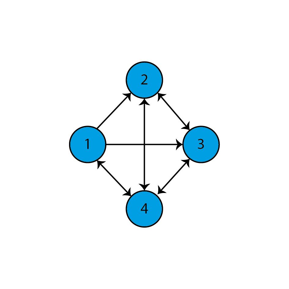
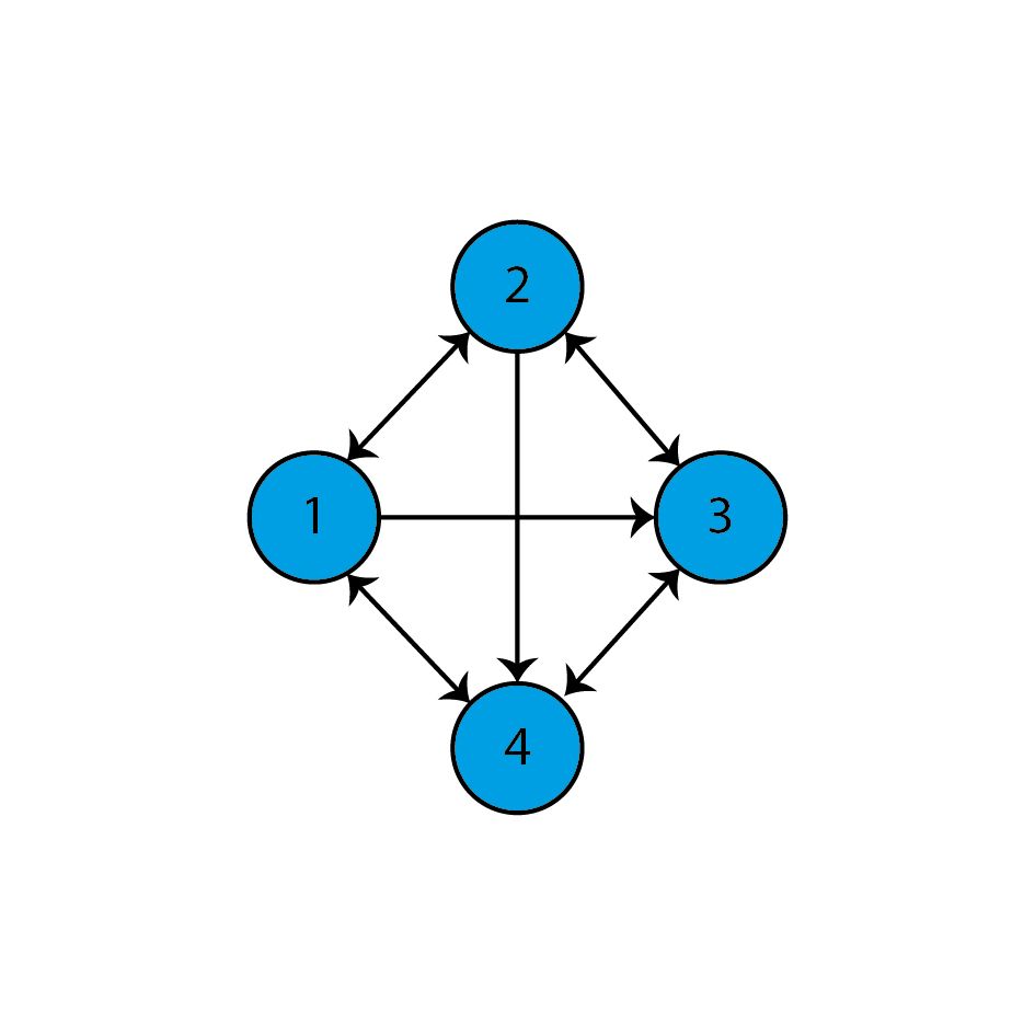
As an illustration, let us consider the multi-agent system that contains 4 nodes depicted in FigureΒ 1. Let the connection between the nodes at a certain time t1subscript𝑑1t_{1} be as in Figure Β 1(a). Subsequently, for some reason the connection between from first to the second agent fails, then the graph loses the directed edge between them at a certain time t2subscript𝑑2t_{2} that is depicted in figure Β 1(b). Hence, the network is time-varying directed graph.
Refer to caption
(a) at time t1subscript𝑑1t_{1}
Refer to caption
(b) at time t2subscript𝑑2t_{2}
Figure 1: Time Varying Directed Network

Having realised the structure of a decentralized multi-agent system, one can move on the problem statement. The task is to sample from a probability distribution that is known up to a normalizing constant. For instance, such a problem arises in Bayesian Inference, when we want to calculate a posterior distribution p​(x|ΞΈ)𝑝conditionalπ‘₯πœƒp(x|\theta) for a set of parameters xπ‘₯x, knowing a prior knowledge p​(x)𝑝π‘₯p(x) and a likelihood p​(ΞΈ|x)𝑝conditionalπœƒπ‘₯p(\theta|x), where ΞΈπœƒ\theta is data. In accordance with the Bayes’ theorem Β (1)

p​(x|ΞΈ)=p​(ΞΈ|x)​p​(x)∫Xp​(ΞΈ|x)​p​(x)​𝑑x,𝑝conditionalπ‘₯πœƒπ‘conditionalπœƒπ‘₯𝑝π‘₯subscript𝑋𝑝conditionalπœƒπ‘₯𝑝π‘₯differential-dπ‘₯\centering p(x|\theta)=\frac{p(\theta|x)p(x)}{\int_{X}p(\theta|x)p(x)dx},\@add@centering (1)

there is a constant in a denominator that constitutes the multiplication of the prior and the likelihood, integrated across the parameters. This integral normalizing constant is typically difficult if not impossible to compute, and hence sampling methods often seek to avoid doing so.

Markov Chain Monte Carlo (MCMC) methods are able to obtain diverse samples from a target posterior distribution. The core of the techniques is to sample a proposal distribution which is then accepted or rejected. There are many variants of these proposal distributions. More recently, it was found that, for especially log concave potentials in general, discretizations of physically motivated stochastic differential equations are able to efficiently for distributions with a high dimension for the parameter xπ‘₯x. One of these proposals is based on Hamiltonian dynamics, which was observed at first in Β [6], while Langevin dynamics underlies another type of proposal, introduced for posterior Bayesian inference with the seminal workΒ [17]. The overdamped Langevin diffusion equation, in particular, arrives at a stationary distribution characterized by a pdf of the form eβˆ’U​(x)/Zsuperscriptπ‘’π‘ˆπ‘₯𝑍e^{-U(x)}/Z, where Z𝑍Z is the normalizing constant, when the diffusion drift term is βˆ‡U​(x)βˆ‡π‘ˆπ‘₯\nabla U(x). This form of potential is common for Gibbs type distributions and likelihood functions arising from exponential families.

Formally, we consider finding the stationary distribution of a pdf wherein there exists a potential given by,

U​(x)=βˆ‘i=1mUi​(x)π‘ˆπ‘₯superscriptsubscript𝑖1π‘šsubscriptπ‘ˆπ‘–π‘₯U(x)=\sum\limits_{i=1}^{m}U_{i}(x)

where for presentation we subsume the dependence on the data ΞΈπœƒ\theta within Ui​(β‹…)subscriptπ‘ˆπ‘–β‹…U_{i}(\cdot), i.e., Ui​(x)=p​(ΞΈi|x)​p​(x)subscriptπ‘ˆπ‘–π‘₯𝑝conditionalsubscriptπœƒπ‘–π‘₯𝑝π‘₯U_{i}(x)=p(\theta_{i}|x)p(x), wherein we drop the normalization constant, and where node i𝑖i knows only the strongly convex function Uisubscriptπ‘ˆπ‘–U_{i}: ℝd→ℝ→superscriptℝ𝑑ℝ\mathbb{R}^{d}\rightarrow\mathbb{R}.

We make the following assumption on {Ui​(β‹…)}subscriptπ‘ˆπ‘–β‹…\{U_{i}(\cdot)\}.

Assumption 1.1.

Each Ui​(x)subscriptπ‘ˆπ‘–π‘₯U_{i}(x) is Lipschitz continuously differentiable with constant L𝐿L, and strongly convex with constant ΞΌπœ‡\mu. Furthermore βˆ‘i=1mUi​(x)superscriptsubscript𝑖1π‘šsubscriptπ‘ˆπ‘–π‘₯\sum\limits_{i=1}^{m}U_{i}(x) is also Lipschitz continuously differentiable and strongly convex with, without loss of generality, the same constants.

2 Background

2.1 The network structure

As described above, the multi-agent system (network) constitutes directed and time-varying connections between nodes with changing in- and out-neighbours. The communication structure is modeled as a graph denoted by 𝒒​(𝒱,β„°)𝒒𝒱ℰ{\mathcal{G}}(\mathcal{V},\mathcal{E}). That is defined as a set of vertex 𝒱𝒱\mathcal{V} = {1,…,m} and we will use ℰ​(t)ℰ𝑑\mathcal{E}(t) to label a set of edges at a certain time t throughout the article.

Let us make some assumptions on the network. It was shown in the related work Β [8], that the property of B-strongly-connectedness is sufficient to derive different bounds on the speed of information propagation. So we require that the sequence {𝒒​(t)}𝒒𝑑\{\mathcal{G}(t)\} is B𝐡B-strongly-connected. In other words, there exists positive integer B𝐡B such that the graph’s edge set is strongly connected for any non-negative kπ‘˜k. Formally:

β„°B​(k)=⋃i=k​B(k+1)​Bβˆ’1ℰ​(i)subscriptβ„°π΅π‘˜subscriptsuperscriptπ‘˜1𝐡1π‘–π‘˜π΅β„°π‘–\mathcal{E}_{B}(k)=\bigcup^{(k+1)B-1}_{i=kB}\mathcal{E}(i)

and the graph 𝒒𝒒\mathcal{G} is connected. Since the observed multi-agent system is directed and time-varying, then one has to introduce in- and out-neighboors for each node i at the current time t.

𝒩ii​n​(t)={j|(j,i)βˆˆβ„°β€‹(t)}βˆͺ{i}superscriptsubscript𝒩𝑖𝑖𝑛𝑑conditional-set𝑗𝑗𝑖ℰ𝑑𝑖\mathcal{N}_{i}^{in}(t)=\{j|(j,i)\in\mathcal{E}(t)\}\cup\{i\}
𝒩io​u​t​(t)={j|(i,j)βˆˆβ„°β€‹(t)}βˆͺ{i}superscriptsubscriptπ’©π‘–π‘œπ‘’π‘‘π‘‘conditional-set𝑗𝑖𝑗ℰ𝑑𝑖\mathcal{N}_{i}^{out}(t)=\{j|(i,j)\in\mathcal{E}(t)\}\cup\{i\}

The authors of the article Β [8] note that the subgradient-push algorithm they developed for decentralized optimization requires only knowledge of out-degree for each node i. So, one should define the out-degree of node i at time t as:

di​(t)=|𝒩io​u​t​(t)|subscript𝑑𝑖𝑑subscriptsuperscriptπ’©π‘œπ‘’π‘‘π‘–π‘‘d_{i}(t)=|\mathcal{N}^{out}_{i}(t)| (2)

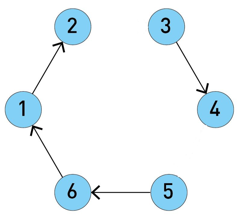
Now, let us introduce the mixing matrix A​(t)𝐴𝑑A(t). As an illustration, consider the graph that is depicted in Figure Β 2.

Refer to caption
(a) The graph
Figure 2: Almost circular graph

This graph is composed of 6 nodes and at this moment it is not fully connected (but is expected to complete its links over time). Taking the first agent, one can see, that it sends his signal to the second agent and itself. Let us then set a11subscriptπ‘Ž11a_{11} equal to 1212\frac{1}{2} and a21subscriptπ‘Ž21a_{21} the same. Continuing, the mixing matrix for the graph is written in Β (3). One can notice, that the sum of elements over any column is equal to 1, so the matrix A​(t)𝐴𝑑A(t) is a column-stochastic.

A​(t)=[120000121210000001200000121000000100000012]𝐴𝑑matrix120000121210000001200000121000000100000012A(t)=\begin{bmatrix}\frac{1}{2}&0&0&0&0&\frac{1}{2}\\ \frac{1}{2}&1&0&0&0&0\\ 0&0&\frac{1}{2}&0&0&0\\ 0&0&\frac{1}{2}&1&0&0\\ 0&0&0&0&1&0\\ 0&0&0&0&0&\frac{1}{2}\end{bmatrix} (3)

We make this assumption formally,

Assumption 2.1.

The mixing matrix A​(t)𝐴𝑑A(t) is column-stochastic for all t𝑑t.

2.2 Elements of spectral theory

Let us present some basic background on the spectral theory of mixing matrices. Introduce the following constants Ξ»πœ†\lambda and δ𝛿\delta associated to a graph sequence 𝒒​(t)𝒒𝑑\mathcal{G}(t). The value of δ𝛿\delta corresponds to, once you continuously multiply the matrices A​(t)𝐴𝑑A(t), the smallest value of an entry of that product matrix. There is always a lower bound and in accordance with assumption V.1 in Β [14], the standard condition is,

Ξ΄β‰₯1mm​B𝛿1superscriptπ‘šπ‘šπ΅\delta\geq\frac{1}{m^{mB}}

One can interpret this as a lower bound on the weight any node assigns to past information from another node.

As for Ξ»πœ†\lambda, for the case of fixed graphs, the variable Ξ»πœ†\lambda will represent the connectivity of the graph, and it is usually the second eigenvalue of the graph adjacency matrix. Usually, the better connected the graph is, the bigger Ξ»πœ†\lambda is, for poorly connected graphs Ξ»πœ†\lambda is almost zero. However, when the graph changes with time, there is no direct interpretation via the eigenvalue, because every graph in the sequence will have a different eigenvalue.Thus one can interpret Ξ»πœ†\lambda in the time-varying case as a lower bound for the connectivity of the time-varying graph.

λ≀(1βˆ’1mm​B)1m​Bπœ†superscript11superscriptπ‘šπ‘šπ΅1π‘šπ΅\lambda\leq\left(1-\frac{1}{m^{mB}}\right)^{\frac{1}{mB}} (4)

2.3 Previous Work

Stochastic Gradient Langevin Dynamics was introduced for posterior Bayesian inference with the seminal workΒ [17].

The paperΒ [4] presented the first application of applying Langevin dynamics, and thus finding a stationary distribution, in the context of a decentralized setting of data distributed across a network. The workΒ [3] extended the framework to consider the momentum based Hamiltonian Langevin dynamics. FinallyΒ [12] considered the problem relaxing the conditions for convexity of the potential (log-concavity of the distribution function) to a log-Sobolev inequality, thus permitting posterior inference for a wider class of decentralized problems.

In regards to decentralized optimization, besides the seminal workΒ [8], there is the paper considering stochastic gradients inΒ [9]. For a nice recent survey on decentralized optimization in machine learning seeΒ [7].

2.4 Probability Distances

In order to present our theoretical results, we must introduce some notation regarding the computation of the distance between two probability distributions. A transference plan ΢​(ΞΌ,Ξ½)πœπœ‡πœˆ\zeta(\mu,\nu) of two probability measures ΞΌπœ‡\mu and ν𝜈\nu on ℬ​(ℝd)ℬsuperscriptℝ𝑑\mathcal{B}(\mathbb{R}^{d}) is itself a probability measure on (ℝd×ℝd,ℬ​(ℝd×ℝd))superscriptℝ𝑑superscriptℝ𝑑ℬsuperscriptℝ𝑑superscriptℝ𝑑(\mathbb{R}^{d}\times\mathbb{R}^{d},\mathcal{B}(\mathbb{R}^{d}\times\mathbb{R}^{d})) that satisfies: for all measurable AβŠ†β„d𝐴superscriptℝ𝑑A\subseteq\mathbb{R}^{d}, it holds that ΢​(A×ℝd)=μ​(A)𝜁𝐴superscriptβ„π‘‘πœ‡π΄\zeta(A\times\mathbb{R}^{d})=\mu(A) and ΢​(ℝdΓ—A)=ν​(A)𝜁superscriptβ„π‘‘π΄πœˆπ΄\zeta(\mathbb{R}^{d}\times A)=\nu(A). We denote by Π​(ΞΌ,Ξ½)Ξ πœ‡πœˆ\Pi(\mu,\nu) the set of transference plans of ΞΌπœ‡\mu and ν𝜈\nu.Two ℝdsuperscriptℝ𝑑\mathbb{R}^{d}-valued random variables (X,Y)π‘‹π‘Œ(X,Y) is a coupling of ΞΌπœ‡\mu and ν𝜈\nu if there exists a ΞΆβˆˆΞ β€‹(ΞΌ,Ξ½)πœΞ πœ‡πœˆ\zeta\in\Pi(\mu,\nu) such that (X,Y)π‘‹π‘Œ(X,Y) are distributed according to ΢𝜁\zeta. The Wasserstein distance of order two is,

W2​(ΞΌ,Ξ½)=(infΞΆβˆˆΞ β€‹(ΞΌ,Ξ½)βˆ«β„d×ℝdβ€–xβˆ’yβ€–2​𝑑΢​(x,y))1/2.subscriptπ‘Š2πœ‡πœˆsuperscriptsubscriptinfimumπœΞ πœ‡πœˆsubscriptsuperscriptℝ𝑑superscriptℝ𝑑superscriptnormπ‘₯𝑦2differential-d𝜁π‘₯𝑦12W_{2}(\mu,\nu)=\left(\inf_{\zeta\in\Pi(\mu,\nu)}\int_{\mathbb{R}^{d}\times\mathbb{R}^{d}}\|x-y\|^{2}d\zeta(x,y)\right)^{1/2}.

For all ΞΌ,Ξ½πœ‡πœˆ\mu,\nu there exists a ΞΆβˆ—βˆˆΞ β€‹(ΞΌ,Ξ½)superscriptπœΞ πœ‡πœˆ\zeta^{*}\in\Pi(\mu,\nu) realizing the infinfimum\inf, i.e., for any coupling (X,Y)π‘‹π‘Œ(X,Y) distributed according to ΞΆβˆ—superscript𝜁\zeta^{*} we have W2​(ΞΌ,Ξ½)=𝔼​[β€–Xβˆ’Yβ€–2]1/2subscriptπ‘Š2πœ‡πœˆπ”Όsuperscriptdelimited-[]superscriptnormπ‘‹π‘Œ212W_{2}(\mu,\nu)=\mathbb{E}[\|X-Y\|^{2}]^{1/2}, defined as the optimal transference plan and optimal coupling associated with W2subscriptπ‘Š2W_{2}. The space 𝒫2​(ℝd)subscript𝒫2superscriptℝ𝑑\mathcal{P}_{2}(\mathbb{R}^{d}) is the set of finite second moment probability measures and together with W2subscriptπ‘Š2W_{2} is a complete separable metric space.

We denote ΞΌβ‰ͺΞ½much-less-thanπœ‡πœˆ\mu\ll\nu to mean that ΞΌπœ‡\mu is absolutely continuous w.r.t. ν𝜈\nu. Recall the Kullback-Leibler (KL) divergence of ΞΌπœ‡\mu from ν𝜈\nu is defined by,

K​L​(ΞΌ|Ξ½)={βˆ«β„dd​μd​ν​(x)​log⁑(d​μd​ν​(x)),if ​μβ‰ͺΞ½,∞otherwise.𝐾𝐿conditionalπœ‡πœˆcasessubscriptsuperscriptβ„π‘‘π‘‘πœ‡π‘‘πœˆπ‘₯π‘‘πœ‡π‘‘πœˆπ‘₯much-less-thanifΒ πœ‡πœˆotherwise.KL(\mu|\nu)=\left\{\begin{array}[]{ll}\int_{\mathbb{R}^{d}}\frac{d\mu}{d\nu}(x)\log\left(\frac{d\mu}{d\nu}(x)\right),&\text{if }\mu\ll\nu,\\ \infty&\text{otherwise.}\end{array}\right.

3 Algorithm

Now, we propose an algorithm to solve the problem of sampling from the target distribution in a decentralized setting with directed graphs. As already mentioned, the perturbed push-sum protocol, which was published in the work Β [8] is at the heart of our developed algorithm. The aspect of the procedure seeking consensus is actually exactly the same. One should take the mixing matrix, which is set by the current graph’s structure, and multiply this matrix A​(t)𝐴𝑑A(t) by the vector of coordinates X𝑋X which is a stack comrpomising of concatenated vectors {X(i)}subscript𝑋𝑖\{X_{(i)}\}, where each X(i)subscript𝑋𝑖X_{(i)} is in turn a stack of components of coordinate on i𝑖i’th node. As soon as we compute the consensus step, then we can compute the balancing vector Y(i)subscriptπ‘Œπ‘–Y_{(i)} for each agent. The (stochastic) gradient is evaluated at another vector Z(i)subscript𝑍𝑖Z_{(i)} that is a balanced weighted average of X(i)subscript𝑋𝑖X_{(i)} and its neighbors, and the update, together with the Gaussian noise, is applied to X(i)subscript𝑋𝑖X_{(i)}.

The set of quantities available and computed by each agent is,

{W(i)​(t),y(i)​(t),Z(i)​(t),X(i)​(t)}subscriptπ‘Šπ‘–π‘‘subscript𝑦𝑖𝑑subscript𝑍𝑖𝑑subscript𝑋𝑖𝑑\left\{W_{(i)}(t),y_{(i)}(t),Z_{(i)}(t),X_{(i)}(t)\right\}

where aside from the scalar y(i)​(t)subscript𝑦𝑖𝑑y_{(i)}(t), all other quantities of d𝑑d-dimensional vectors.

We now present the specific Algorithm, as inspired by the merging of the perturbed push sum approach given inΒ [8] and the unadjusted Langevin algorithm, as described for instance inΒ [2].

The Algorithm, from the perspective of agent i𝑖i, is defined as follows. To begin with, we set, for all i𝑖i, the quantities,

{W(i)​(0),Z(i)​(0),X(i)​(0)}subscriptπ‘Šπ‘–0subscript𝑍𝑖0subscript𝑋𝑖0\left\{W_{(i)}(0),Z_{(i)}(0),X_{(i)}(0)\right\}

to zero and y(i)​(0)=1subscript𝑦𝑖01y_{(i)}(0)=1. Recall that at each iteration di​(t)subscript𝑑𝑖𝑑d_{i}(t) is defined byΒ (2). Each agent i𝑖i iterates the set of equationsΒ (5)

{W(i)​(t+1)=βˆ‘jβˆˆπ’©ii​n​(t)X(j)​(t)dj​(t)Y(i)​(t+1)=βˆ‘jβˆˆπ’©ii​n​(t)Y(j)​(t)dj​(t)Z(i)​(t+1)=W(i)​(t+1)Y(i)​(t+1)X(i)​(t+1)=βˆ‘jβˆˆπ’©ii​n​(t)X(j)​(t)dj​(t)βˆ’Ξ±(t+1)βˆ‡U(i)(Z(i)(t+1)))+2​α​(t+1)​B(i)​(t+1)\begin{cases}\begin{array}[]{l}W_{(i)}(t+1)=\sum\limits_{j\in\mathcal{N}_{i}^{in}(t)}\frac{X_{(j)}(t)}{d_{j}(t)}\\ Y_{(i)}(t+1)=\sum\limits_{j\in\mathcal{N}_{i}^{in}(t)}\frac{Y_{(j)}(t)}{d_{j}(t)}\\ Z_{(i)}(t+1)=\frac{W_{(i)}(t+1)}{Y_{(i)}(t+1)}\\ X_{(i)}(t+1)=\sum\limits_{j\in\mathcal{N}_{i}^{in}(t)}\frac{X_{(j)}(t)}{d_{j}(t)}\\ \qquad-\alpha(t+1)\nabla U_{(i)}(Z_{(i)}(t+1)))\\ \qquad+\sqrt{2\alpha(t+1)}B_{(i)}(t+1)\end{array}\end{cases} (5)

where we denote B(i)​(t+1)=α​(t+1)​ξ(i)​(t+1)+R(i)​(t+1)subscript𝐡𝑖𝑑1𝛼𝑑1subscriptπœ‰π‘–π‘‘1subscript𝑅𝑖𝑑1B_{(i)}(t+1)=\sqrt{\alpha(t+1)}\xi_{(i)}(t+1)+R_{(i)}(t+1), with ξ​(t+1)πœ‰π‘‘1\xi(t+1) is a zero bias bounded variance stochastic gradient error and R(i)​(t+1)subscript𝑅𝑖𝑑1R_{(i)}(t+1) is an isotropic Gaussian random variable. Let us set α​(t+1)≀1/Οƒ2:=1/𝔼​‖ξ‖𝛼𝑑11superscript𝜎2assign1𝔼normπœ‰\sqrt{\alpha(t+1)}\leq 1/\sigma^{2}:=1/\mathbb{E}\|\xi\| so that the standard deviation associated with 2​αt​B​(t+1)2subscript𝛼𝑑𝐡𝑑1\sqrt{2\alpha_{t}}B(t+1) is always less than 2.

Let us now consider the iterations on the full stack of vectors {X,Y,Z}π‘‹π‘Œπ‘\{X,Y,Z\} using the mixing matrix A𝐴A,

{Y​(t+1)=A​(t)​Y​(t)Z​(t+1)=A​(t)​X​(t)⊘A​(t)​Y​(t)X​(t+1)=A​(t)​X​(t)βˆ’Ξ±β€‹(t+1)β€‹βˆ‡U~​(Z​(t+1))+2​α​(t+1)​Bt+1casesπ‘Œπ‘‘1π΄π‘‘π‘Œπ‘‘π‘π‘‘1βŠ˜π΄π‘‘π‘‹π‘‘π΄π‘‘π‘Œπ‘‘π‘‹π‘‘1𝐴𝑑𝑋𝑑𝛼𝑑1βˆ‡~π‘ˆπ‘π‘‘12𝛼𝑑1subscript𝐡𝑑1otherwise\begin{cases}\begin{array}[]{l}Y(t+1)=A(t)Y(t)\\ Z(t+1)={A(t)X(t)}\oslash{A(t)Y(t)}\\ X(t+1)=A(t)X(t)-\alpha(t+1)\nabla\tilde{U}(Z(t+1))\\ +\sqrt{2\alpha(t+1)}B_{t+1}\end{array}\end{cases} (6)

where we are defining,

βˆ‡U~​(Z)=(βˆ‡U1​(Z(1))β€¦βˆ‡Ui​(Z(i)).,.βˆ‡Um​(Z(m)))βˆ‡~π‘ˆπ‘matrixβˆ‡subscriptπ‘ˆ1subscript𝑍1β€¦βˆ‡subscriptπ‘ˆπ‘–subscript𝑍𝑖absentβˆ‡subscriptπ‘ˆπ‘šsubscriptπ‘π‘š\nabla\tilde{U}(Z)=\begin{pmatrix}\nabla U_{1}(Z_{(1)})\\ ...\\ \nabla U_{i}(Z_{(i)})\\ .,.\\ \nabla U_{m}(Z_{(m)})\end{pmatrix}

and we abuse notation with letting [X⊘Y](i)=X(i)/y(i)subscriptdelimited-[]βŠ˜π‘‹π‘Œπ‘–subscript𝑋𝑖subscript𝑦𝑖[X\oslash Y]_{(i)}=X_{(i)}/y_{(i)}

In the theory (and of course the numerical implementation), we shall consider the discretization, however, out of mathematical interest, we can note that, considering the form of the Euler-Maruyama (EM) discretization, writing A(t)X(t)=A(t)X(t)+X(t)βˆ’X(t)=(A(t)βˆ’I)X(t)+X(t))A(t)X(t)=A(t)X(t)+X(t)-X(t)=(A(t)-I)X(t)+X(t)), we can notice, out of mathematical interest, that this corresponds to the EM discretization of the dynamics given by (where we now overload t𝑑t to be continuous),

Zt=(At​Xt)⊘(At​Yt)d​Yt=(Atβˆ’I)​Ytd​Xt=(Atβˆ’I)​Xtβˆ’Ξ±tβ€‹βˆ‡U~​(Zt)+2​αt​d​Btsubscriptπ‘π‘‘βŠ˜subscript𝐴𝑑subscript𝑋𝑑subscript𝐴𝑑subscriptπ‘Œπ‘‘π‘‘subscriptπ‘Œπ‘‘subscript𝐴𝑑𝐼subscriptπ‘Œπ‘‘π‘‘subscript𝑋𝑑subscript𝐴𝑑𝐼subscript𝑋𝑑subscriptπ›Όπ‘‘βˆ‡~π‘ˆsubscript𝑍𝑑2subscript𝛼𝑑𝑑subscript𝐡𝑑\begin{array}[]{l}Z_{t}=(A_{t}X_{t})\oslash(A_{t}Y_{t})\\ dY_{t}=(A_{t}-I)Y_{t}\\ dX_{t}=(A_{t}-I)X_{t}-\alpha_{t}\nabla\tilde{U}(Z_{t})+\sqrt{2\alpha_{t}}dB_{t}\end{array}

where d​Bt𝑑subscript𝐡𝑑dB_{t} is a Brownian motion term and clearly the discretization is with a step-size of one. Unlike other works in Langevin dynamics, we do not analyze the SDE directly but only its discretization, however.

4 Theoretical Results

We present the sequence of Lemmas and our final convergence result in measure for the Algorithm defined in SectionΒ 3. The proofs of the statements are left to the Supplementary Material.

First we will require a bound in expectation on the gradient vectors, which we derive by deriving a bound on the expectation of the norm of the vectors on which they are evaluated, Z(i)​(t)subscript𝑍𝑖𝑑Z_{(i)}(t).

Lemma 4.1.

It holds that there exists some compact set 𝒲𝒲\mathcal{W} such that for all i𝑖i

𝔼​‖X(i)​(t+1)Y(i)​(t+1)‖≀{β€–Z(i)​(t+1)β€–if ​Z(i)​(t+1)βˆˆπ’²Rotherwise𝔼normsubscript𝑋𝑖𝑑1subscriptπ‘Œπ‘–π‘‘1casesnormsubscript𝑍𝑖𝑑1ifΒ subscript𝑍𝑖𝑑1𝒲𝑅otherwise\mathbb{E}\left\|\frac{X_{(i)}(t+1)}{Y_{(i)}(t+1)}\right\|\leq\left\{\begin{array}[]{lr}\|Z_{(i)}(t+1)\|&\text{if }Z_{(i)}(t+1)\in\mathcal{W}\\ R&\text{otherwise}\end{array}\right.

with R𝑅R depending on 𝒲𝒲\mathcal{W} and problem constants.

Lemma 4.2.

It holds that there exists a C𝐢C such that,

π”Όβ€‹β€–βˆ‡Ui​(Z(i)​(t+1))‖≀C𝔼normβˆ‡subscriptπ‘ˆπ‘–subscript𝑍𝑖𝑑1𝐢\mathbb{E}\|\nabla U_{i}(Z_{(i)}(t+1))\|\leq C

The next statement is the same as Corollary 1 inΒ [9], where we recall that Ξ»πœ†\lambda is a graph-structure related constant satisfyingΒ (4) which implies that Ξ»<1πœ†1\lambda<1,

Lemma 4.3.

It holds that,

β€–Z(i)​(t+1)βˆ’βˆ‘i=1mX(i)​(t)m‖≀8δ​(Ξ»tβ€‹βˆ‘i=1mβ€–X(i)​(0)β€–1+βˆ‘s=1tΞ»tβˆ’sβ€‹βˆ‘i=1mβ€–ei​(s)β€–)normsubscript𝑍𝑖𝑑1superscriptsubscript𝑖1π‘šsubscriptπ‘‹π‘–π‘‘π‘šabsent8𝛿superscriptπœ†π‘‘superscriptsubscript𝑖1π‘šsubscriptnormsubscript𝑋𝑖01superscriptsubscript𝑠1𝑑superscriptπœ†π‘‘π‘ superscriptsubscript𝑖1π‘šnormsubscript𝑒𝑖𝑠\begin{array}[]{l}\left\|Z_{(i)}(t+1)-\frac{\sum\limits_{i=1}^{m}X_{(i)}(t)}{m}\right\|\\ \qquad\leq\frac{8}{\delta}\left(\lambda^{t}\sum\limits_{i=1}^{m}\|X_{(i)}(0)\|_{1}+\sum\limits_{s=1}^{t}\lambda^{t-s}\sum\limits_{i=1}^{m}\left\|e_{i}(s)\right\|\right)\end{array}

where,

ei(s)=Ξ±(s+1)βˆ‡Ui(Z(i)(s+1)))+2​α​(s+1)B(i)(s+1)e_{i}(s)=\alpha(s+1)\nabla U_{i}(Z_{(i)}(s+1)))+\sqrt{2\alpha(s+1)}B_{(i)}(s+1)

This together with LemmaΒ 4.2 allows us to prove the following bound on the running sum of the consensus error.

Lemma 4.4.
𝔼​[βˆ‘t=1Ο„β€–Z(i)​(t+1)βˆ’βˆ‘i=1mX(i)​(t)mβ€–]≀8δ​λ1βˆ’Ξ»β€‹βˆ‘i=1mβ€–X(i)​(0)β€–1+8δ​D​m1βˆ’Ξ»β€‹(1+Ο„)𝔼delimited-[]superscriptsubscript𝑑1𝜏normsubscript𝑍𝑖𝑑1superscriptsubscript𝑖1π‘šsubscriptπ‘‹π‘–π‘‘π‘šabsent8π›Ώπœ†1πœ†superscriptsubscript𝑖1π‘šsubscriptnormsubscript𝑋𝑖018π›Ώπ·π‘š1πœ†1𝜏\begin{array}[]{l}\mathbb{E}\left[\sum\limits_{t=1}^{\tau}\left\|Z_{(i)}(t+1)-\frac{\sum\limits_{i=1}^{m}X_{(i)}(t)}{m}\right\|\right]\\ \qquad\leq\frac{8}{\delta}\frac{\lambda}{1-\lambda}\sum\limits_{i=1}^{m}\|X_{(i)}(0)\|_{1}+\frac{8}{\delta}\frac{Dm}{1-\lambda}(1+\sqrt{\tau})\end{array}

Now define,

X¯​(t)=βˆ‘i=1mX(i)​(t)m¯𝑋𝑑superscriptsubscript𝑖1π‘šsubscriptπ‘‹π‘–π‘‘π‘š\bar{X}(t)=\frac{\sum\limits_{i=1}^{m}X_{(i)}(t)}{m}

we have, by the column-stochasticity of A​(t)𝐴𝑑A(t),

X¯​(t+1)=X¯​(t)βˆ’Ξ±β€‹(t+1)mβ€‹βˆ‘i=1mβˆ‡U​(X¯​(t))+α​(t+1)mβ€‹βˆ‘i=1m(βˆ‡U​(X¯​(t))βˆ’U​(Z(i)​(t+1)))+B¯​(t+1)¯𝑋𝑑1¯𝑋𝑑𝛼𝑑1π‘šsuperscriptsubscript𝑖1π‘šβˆ‡π‘ˆΒ―π‘‹π‘‘π›Όπ‘‘1π‘šsuperscriptsubscript𝑖1π‘šβˆ‡π‘ˆΒ―π‘‹π‘‘π‘ˆsubscript𝑍𝑖𝑑1¯𝐡𝑑1\begin{array}[]{l}\bar{X}(t+1)=\bar{X}(t)-\frac{\alpha(t+1)}{m}\sum\limits_{i=1}^{m}\nabla U(\bar{X}(t))\\ \qquad+\frac{\alpha(t+1)}{m}\sum\limits_{i=1}^{m}\left(\nabla U(\bar{X}(t))-U(Z_{(i)}(t+1))\right)+\bar{B}(t+1)\end{array} (7)

LemmaΒ 4.4 implies the following,

Corollary 4.4.1.

Given any Ξ³>0𝛾0\gamma>0, there exists CΞ³>0subscript𝐢𝛾0C_{\gamma}>0 such that,

Eβˆ₯XΒ―(t))βˆ’Z(i)(t+1)βˆ₯≀CΞ³t1/2βˆ’Ξ³E\|\bar{X}(t))-Z_{(i)}(t+1)\|\leq\frac{C_{\gamma}}{t^{1/2-\gamma}}

Let Ξ½Β―tsubscriptΒ―πœˆπ‘‘\bar{\nu}_{t} be the distribution associated with X¯​(t)¯𝑋𝑑\bar{X}(t)

We are now ready to use the arguments inΒ [1] regarding perturbed Langevin methods. In particular, we can apply Proposition 2 to state that,

Lemma 4.5.
W2​(Ξ½Β―t+1,Ο€)≀ρt+1​W2​(Ξ½Β―t,Ο€)+1.65​L​(Ξ±t+13​d)1/2+α​(t+1)​d​Lβ€‹βˆ‘i=1m𝔼​‖X¯​(t)βˆ’Z(i)​(t+1)β€–subscriptπ‘Š2subscriptΒ―πœˆπ‘‘1πœ‹subscriptπœŒπ‘‘1subscriptπ‘Š2subscriptΒ―πœˆπ‘‘πœ‹1.65𝐿superscriptsuperscriptsubscript𝛼𝑑13𝑑12𝛼𝑑1𝑑𝐿superscriptsubscript𝑖1π‘šπ”Όnorm¯𝑋𝑑subscript𝑍𝑖𝑑1\begin{array}[]{l}W_{2}(\bar{\nu}_{t+1},\pi)\leq\rho_{t+1}W_{2}(\bar{\nu}_{t},\pi)+1.65L(\alpha_{t+1}^{3}d)^{1/2}\\ \qquad+\alpha(t+1)\sqrt{d}L\sum\limits_{i=1}^{m}\mathbb{E}\|\bar{X}(t)-Z_{(i)}(t+1)\|\end{array}

where ρt+1=max⁑(1βˆ’ΞΌβ€‹Ξ±β€‹(t+1),L​α​(t+1)βˆ’1)subscriptπœŒπ‘‘11πœ‡π›Όπ‘‘1𝐿𝛼𝑑11\rho_{t+1}=\max(1-\mu\alpha(t+1),L\alpha(t+1)-1).

Now recall

Lemma 4.6.

[13, Lemma 2.4] Let ukβ‰₯0subscriptπ‘’π‘˜0u_{k}\geq 0 and,

uk+1≀(1βˆ’ck)​uk+dkp+1subscriptπ‘’π‘˜11π‘π‘˜subscriptπ‘’π‘˜π‘‘superscriptπ‘˜π‘1u_{k+1}\leq\left(1-\frac{c}{k}\right)u_{k}+\frac{d}{k^{p+1}}

with d>0𝑑0d>0, p>0𝑝0p>0 and c>0𝑐0c>0 and c>p𝑐𝑝c>p. Then,

uk≀d​(cβˆ’p)βˆ’1​kβˆ’p+o​(kβˆ’p)subscriptπ‘’π‘˜π‘‘superscript𝑐𝑝1superscriptπ‘˜π‘π‘œsuperscriptπ‘˜π‘u_{k}\leq d(c-p)^{-1}k^{-p}+o(k^{-p})

Apply the previous two Lemmas together with CorollaryΒ 4.4.1 to conclude,

Theorem 4.7.

Let α​(0)≀min⁑{12​L,ΞΌ4​L2}𝛼012πΏπœ‡4superscript𝐿2\alpha(0)\leq\min\left\{\frac{1}{2L},\frac{\mu}{4L^{2}}\right\} and α​(t)=α​(0)/(1+t)𝛼𝑑𝛼01𝑑\alpha(t)=\alpha(0)/(1+t). We have that,

W2​(Ξ½Β―k+1,Ο€)≀(Cγ​m+1.65)​L​d1/2(μ​α​(0)βˆ’1/2+Ξ³)​(1+t)(1/2βˆ’Ξ³)+Ξ²ksubscriptπ‘Š2subscriptΒ―πœˆπ‘˜1πœ‹subscriptπΆπ›Ύπ‘š1.65𝐿superscript𝑑12πœ‡π›Ό012𝛾superscript1𝑑12𝛾subscriptπ›½π‘˜W_{2}(\bar{\nu}_{k+1},\pi)\leq\frac{(C_{\gamma}m+1.65)Ld^{1/2}}{(\mu\alpha(0)-1/2+\gamma)(1+t)^{(1/2-\gamma)}}+\beta_{k}

where Ξ²k=o​((1+t)βˆ’(1/2βˆ’Ξ³))subscriptπ›½π‘˜π‘œsuperscript1𝑑12𝛾\beta_{k}=o\left((1+t)^{-(1/2-\gamma)}\right)

5 Numerical Experiments

5.1 Notes on Parameter Tuning

There is a classical practical question in regards to implementing SGLD algorithms for sampling–how do we tune the step-size, considering its dual influence on the convergence as well as the variance of Brownian term? There are some papers, whose main goals are to study the question. The first mentioned related work Β [11] solves the problem via finding the choice that minimizes the asymptotic KL-divergence. However, it applies only in the case of independent proposal distributions, when new samples are generated regardless of the history. Thus, applying such approach to classic proposals as Random Walk Metropolis (RWM) or Metropolis-Hastings adjusted Langevin algorithm (MALA), it leads to a collapsed delta function solution. Recently, another article Β [16] was published extendingΒ [11]. Optimizing a special speed measure ((2) in Β [16]), one can obtain the algorithm which can tune the optimal step-size as well as covariance matrix for the best convergence. Also, it is worth noticing, that entropy is at the heart of Titsias’s approach. However, entropy is not the only way to solve such problems. For instance, Β [15] and Β [5] use other methods to get optimal parameters, although the second paper applies their method for HMC. However, we prefer to pick out the Titsias’s approach for obtaining optimal step-sizes in our algorithm.

5.2 Bayesian Linear Regression

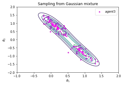
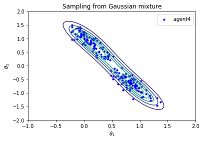
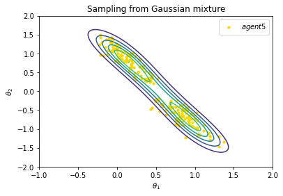
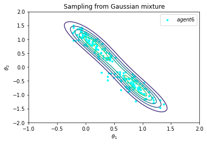
In this subsection, we study the algorithm’s ability to converge to a desired distribution arising from Bayesian Linear Regression. We consider a multi-agent network composed of 4 nodes. Classical linear regression is described by the following expression:

y=X​w+δ𝑦𝑋𝑀𝛿y=Xw+\delta

where y𝑦y constitutes a target variable and the noise is denoted by δ𝛿\delta, whereas X𝑋X and w𝑀w are a set of features and weights of the linear model, respectively. We can generate data as follows:

Ξ΄βˆΌπ’©β€‹(0,Οƒ2),XjβˆΌπ’©β€‹(0,I1)βˆ€jformulae-sequencesimilar-to𝛿𝒩0superscript𝜎2similar-tosubscript𝑋𝑗𝒩0subscript𝐼1for-all𝑗\delta\sim\mathcal{N}(0,\sigma^{2}),\quad X_{j}\sim\mathcal{N}(0,I_{1})\quad\forall j

We generate 800 samples and separate 200 samples across each of four machines. Thus, each agent is going to process its 200 samples, not having access to samples of the other agents. Our main goal is to get the posterior distribution of weights. However, to facilitate the problem we are going to use ”poor” Bayesian inference. In other words, one would like to find out the mode of the posterior distribution. Since we use Bayesian linear regression, we should introduce a prior distribution for weights. Implying features’ equal a priori significance, we choose a zero-mean standard normal distribution with an identity 2 dimensional covariance matrix. Recall Bayes’s theorem as follows:

p​(w|X,y)=p​(y|X,w)​p​(w)∫wp​(y|X,w)​p​(w)​𝑑w𝑝conditional𝑀𝑋𝑦𝑝conditional𝑦𝑋𝑀𝑝𝑀subscript𝑀𝑝conditional𝑦𝑋𝑀𝑝𝑀differential-d𝑀p(w|X,y)=\frac{p(y|X,w)p(w)}{\int_{w}p(y|X,w)p(w)dw}

where p​(w)𝑝𝑀p(w) constitutes the prior distribution for weights, while p​(y|X,w)𝑝conditional𝑦𝑋𝑀p(y|X,w) is a likelihood of data. In the experiment, each node will take its own mini-batch, whose size is equal to 1, will calculate consensus step and point where we take the gradient. Having done these computations, each node samples a new object from the posterior distribution of weights. Since our posterior distribution is a multivariate normal distribution and a distribution that makes a current sample on a node is the same, one can calculate the second Wasserstein distance between this distributions analytically as follows:

𝒲2​(𝒩​(m1,Ξ£1),𝒩​(m2,Ξ£2))=β€–m1βˆ’m2β€–+β€–Ξ£112βˆ’Ξ£212β€–subscript𝒲2𝒩subscriptπ‘š1subscriptΞ£1𝒩subscriptπ‘š2subscriptΞ£2normsubscriptπ‘š1subscriptπ‘š2normsuperscriptsubscriptΞ£112superscriptsubscriptΞ£212\mathcal{W}_{2}(\mathcal{N}(m_{1},\Sigma_{1}),\mathcal{N}(m_{2},\Sigma_{2}))=\|m_{1}-m_{2}\|+\|\Sigma_{1}^{\frac{1}{2}}-\Sigma_{2}^{\frac{1}{2}}\|

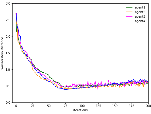
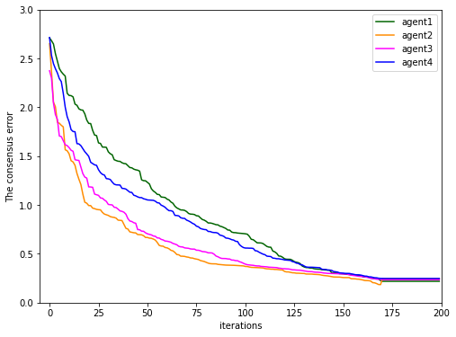
Thus, we repeat this process for 200 iterations (1 batch per one iteration, i.e., one epoch), sometimes changing the set of edges. In figure Β 3(a), one can look at the final plot that deals with the convergence between distributions in terms of the second Wasserstein distance. Meanwhile, one can see the consensus error for each one from 4 agents in figure Β 3(b).

Refer to caption
(a) The 2nd Wasserstein distance
Refer to caption
(b) The consensus error
Figure 3: The Second Wasserstein Distance and the consensus error in case of Bayesian linear regression

5.3 Sampling from Gaussian mixture

In this subsection, we illustrate an experiment that deals with sampling from a multi-modal probability distribution. Recall the definition of a Gaussian mixture:

βˆ‘k=1nΟ•k​𝒩​(mk,Ξ£k)superscriptsubscriptπ‘˜1𝑛subscriptitalic-Ο•π‘˜π’©subscriptπ‘šπ‘˜subscriptΞ£π‘˜\sum_{k=1}^{n}\phi_{k}\mathcal{N}(m_{k},\Sigma_{k})

where a the mixture constants Ο•ksubscriptitalic-Ο•π‘˜\phi_{k} satisfy βˆ‘k=1nΟ•ksuperscriptsubscriptπ‘˜1𝑛subscriptitalic-Ο•π‘˜\sum_{k=1}^{n}\phi_{k} = 1. Let us consider a mixture of two one-dimensional Gaussian distributions under the assumption that their standard deviations are known, but not their means. However, there are some prior distributions for the means of both Gaussians. Then, we get for each sample xisubscriptπ‘₯𝑖x_{i}, that:

xi∼12​𝒩​(ΞΈ1,Οƒx2)+12​𝒩​(ΞΈ1+ΞΈ2,Οƒx2)similar-tosubscriptπ‘₯𝑖12𝒩subscriptπœƒ1superscriptsubscript𝜎π‘₯212𝒩subscriptπœƒ1subscriptπœƒ2superscriptsubscript𝜎π‘₯2x_{i}\sim\frac{1}{2}\mathcal{N}(\theta_{1},\sigma_{x}^{2})+\frac{1}{2}\mathcal{N}(\theta_{1}+\theta_{2},\sigma_{x}^{2}) (8)

where Οƒx2superscriptsubscript𝜎π‘₯2\sigma_{x}^{2} equals to 2. As for prior distributions, they will be as below:

ΞΈ1βˆΌπ’©β€‹(0,Οƒ12),ΞΈ2βˆΌπ’©β€‹(0,Οƒ22)formulae-sequencesimilar-tosubscriptπœƒ1𝒩0superscriptsubscript𝜎12similar-tosubscriptπœƒ2𝒩0superscriptsubscript𝜎22\theta_{1}\sim\mathcal{N}(0,\sigma_{1}^{2}),\theta_{2}\sim\mathcal{N}(0,\sigma_{2}^{2})

where Οƒ12superscriptsubscript𝜎12\sigma_{1}^{2} and Οƒ22superscriptsubscript𝜎22\sigma_{2}^{2} equal to 10 and 1 respectively. Now, one can fix ΞΈ1subscriptπœƒ1\theta_{1} = 0 and ΞΈ2subscriptπœƒ2\theta_{2} = 1. Thus, having fixed values of means, we get the certain mixture of two Gaussian distributions. In this experiment, we consider a decentralized system that is composed of 4 nodes. Then, one can generate 800 samples from the distribution of xisubscriptπ‘₯𝑖x_{i} defined above (8) with these given ΞΈ1subscriptπœƒ1\theta_{1} and ΞΈ2subscriptπœƒ2\theta_{2} and randomly and separate the samples evenly across the network.

Then, the main goal of the experiment is to propose a posterior distribution for ΞΈ1subscriptπœƒ1\theta_{1} and ΞΈ2subscriptπœƒ2\theta_{2} from the set of samples, specifically,:

p​(ΞΈβ†’|X,Οƒx,Οƒ1,Οƒ2)∼[∏i=1np​(Xi|ΞΈβ†’,Οƒx)]​p​(ΞΈβ†’|Οƒ1,Οƒ2)similar-to𝑝conditionalβ†’πœƒπ‘‹subscript𝜎π‘₯subscript𝜎1subscript𝜎2delimited-[]superscriptsubscriptproduct𝑖1𝑛𝑝conditionalsubscriptπ‘‹π‘–β†’πœƒsubscript𝜎π‘₯𝑝conditionalβ†’πœƒsubscript𝜎1subscript𝜎2p(\vec{\theta}|X,\sigma_{x},\sigma_{1},\sigma_{2})\sim[\prod_{i=1}^{n}p(X_{i}|\vec{\theta},\sigma_{x})]p(\vec{\theta}|\sigma_{1},\sigma_{2})

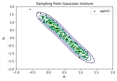
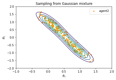
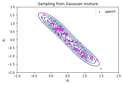
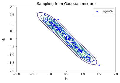
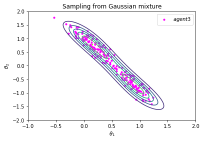
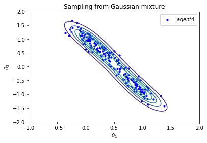
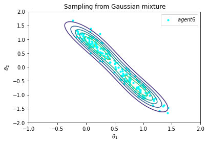
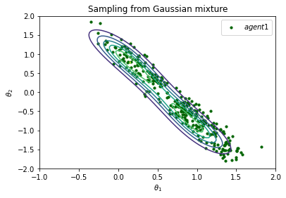
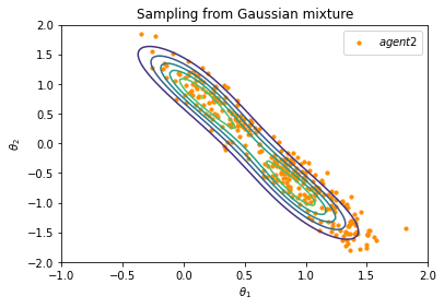
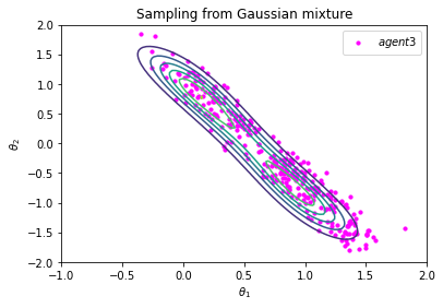
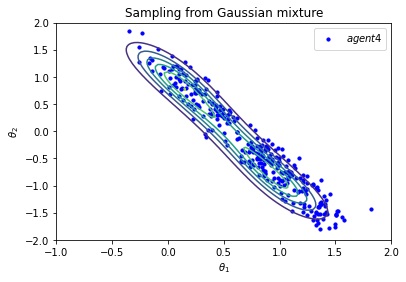
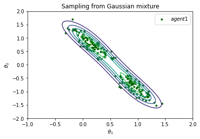
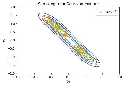
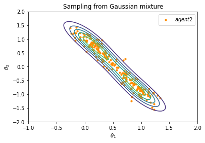
Using MCMC methods and taking the gradients of the joint log-likelihood, one can obtain samples from a desired distribution. We apply the Algorithm given inΒ (5), where we take the gradient of a joint log-likelihood, for each node, for its set of samples, along with the consensus step at each iteration.. The step-size is diminishing and is taken as α​(t)=a(b+t)Ξ³π›Όπ‘‘π‘Žsuperscript𝑏𝑑𝛾\alpha(t)=\frac{a}{(b+t)^{\gamma}}, where γ𝛾\gamma equals to 0.65, when a and b are set such that α​(t)𝛼𝑑\alpha(t) is changed from 0.01 to 0.0001. In FigureΒ 4: (a) - (d), one can see how each agent is able to sample from Gaussian mixture posterior distribution above.
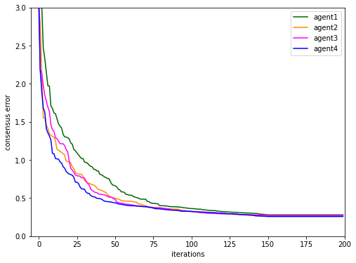
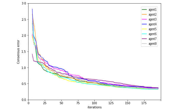
Moreover, one would like to look at an error between each node and average over all nodes on each iteration. Such difference between ”average” node and an agent of decentralized network one can call as ”the consensus error”. In other words, ”Tte consensus error” shows up at all the following expression on each iteration for each node in the multi-agent network:

β€–X(i)​(t)βˆ’X¯​(t)β€–2superscriptnormsubscript𝑋𝑖𝑑¯𝑋𝑑2\|X_{(i)}(t)-\bar{X}(t)\|^{2}

Thus, one should take values, which are generated by the algorithm from i𝑖i’th node, and calculate the squared difference on each t𝑑t iteration. One can look at the consensus error for 4 agents in case of sampling from Gaussian mixture in FigureΒ 4(e).

Refer to caption
(a) agent 1
Refer to caption
(b) agent 2
Refer to caption
(c) agent 3
Refer to caption
(d) agent 4
Refer to caption
(e) The consensus error
Figure 4: (a) -(d) :The sampling from Gaussian mixture for 4 agents, (e) - The consensus error for 4 agents

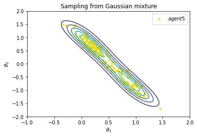
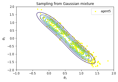
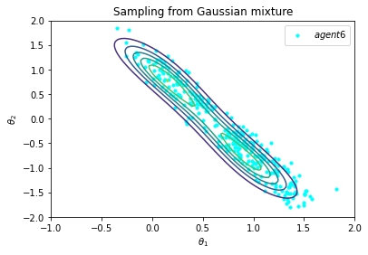
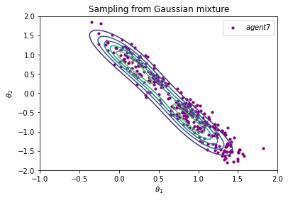
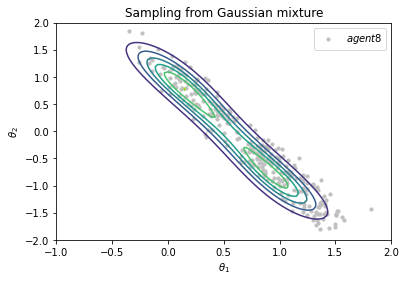
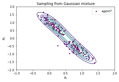
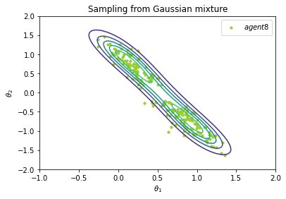
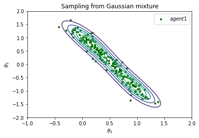
We have included results for sampling from a Gaussian mixture in decentralized settings with 8 nodes. FigureΒ 6 displays the results. One can observe the following expected fact. The more agents takes part in Bayesian logistic regression with decentralized settings, the less variance of accuracy and the faster convergence to the consensus accuracy. The same results are in the experiment for sampling from Gaussian mixture. The more agents are in decentralized settings, the more clearly are seen the two modes of this distribution.
Refer to caption
(a) agent 1
Refer to caption
(b) agent 2
Refer to caption
(c) agent 3
Refer to caption
(d) agent 4
Refer to caption
(e) agent 5
Refer to caption
(f) agent 6
Figure 5: Samples from SGLD in case of sampling from Gaussian mixture by 6 agents
Refer to caption
(a) agent 1
Refer to caption
(b) agent 2
Refer to caption
(c) agent 3
Refer to caption
(d) agent 4
Refer to caption
(e) agent 5
Refer to caption
(f) agent 6
Refer to caption
(g) agent 7
Refer to caption
(h) agent 8
Refer to caption
(i) consensus
Figure 6: Samples from SGLD and the Consensus error in case of sampling from Gaussian mixture by 8 agents
Refer to caption
(a) agent 1
Refer to caption
(b) agent 2
Refer to caption
(c) agent 3
Refer to caption
(d) agent 4
Refer to caption
(e) agent 5
Refer to caption
(f) agent 6
Refer to caption
(g) agent 7
Refer to caption
(h) agent 8
Refer to caption
(i) agent 9
Refer to caption
(j) agent 10
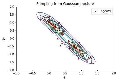
Figure 7: Samples from SGLD in case of sampling from Gaussian mixture by 10 agents

5.4 Bayesian Logistic Regression

In the final subsection, we apply our algorithm, which is based on stochastic gradient Langevin algorithm, to a case of Bayesian logistic regression for real data. Specifically we consider the problem of binary classification, with a target variable y ∈{βˆ’1,1}absent11\in\{-1,1\}. The a9a data-test is a huge-scale and classic data-set for binary classification. This data-set is available at the UCI machine learning repository. It is composed of 32561 samples and 123 features. Each feature has 2 unique values 1 or 0, whereas the target variable has values 1 and -1. In this experiment our decentralized setting is composed of 4 agents. Then, we take 80% of data as train data-set and separate between nodes equally and randomly.

We have the following expression for the posterior for N𝑁N observations:

π​(w)=p​(w|x,y)=1Cβ€‹βˆi=1Np​(yi|xi,w)​p​(w)πœ‹π‘€π‘conditional𝑀π‘₯𝑦1𝐢superscriptsubscriptproduct𝑖1𝑁𝑝conditionalsubscript𝑦𝑖subscriptπ‘₯𝑖𝑀𝑝𝑀\pi(w)=p(w|x,y)=\frac{1}{C}\prod_{i=1}^{N}p(y_{i}|x_{i},w)p(w)

where C is a normalizing constant. Then we takeΒ (5) with βˆ‡Ui​(Z)=βˆ‡(∏i∈Siβˆ’log⁑p​(yi|xi,Z)​p​(Z))βˆ‡subscriptπ‘ˆπ‘–π‘βˆ‡subscriptproduct𝑖subscript𝑆𝑖𝑝conditionalsubscript𝑦𝑖subscriptπ‘₯𝑖𝑍𝑝𝑍\nabla U_{i}(Z)=\nabla\left(\prod_{i\in S_{i}}-\log p(y_{i}|x_{i},Z)p(Z)\right) where SiβŠ†[N]subscript𝑆𝑖delimited-[]𝑁S_{i}\subseteq[N] the subset of data given to agent i𝑖i. One can write the expression for the gradient of potential function as follows:

βˆ‡U​(z)=βˆ‘i=1myi​xi1+eβˆ’yi​zT​xiβˆ’s​i​g​n​(z)βˆ‡π‘ˆπ‘§superscriptsubscript𝑖1π‘šsubscript𝑦𝑖subscriptπ‘₯𝑖1superscript𝑒subscript𝑦𝑖superscript𝑧𝑇subscriptπ‘₯𝑖𝑠𝑖𝑔𝑛𝑧\nabla U(z)=\sum_{i=1}^{m}\frac{y_{i}x_{i}}{1+e^{-y_{i}z^{T}x_{i}}}-sign(z)

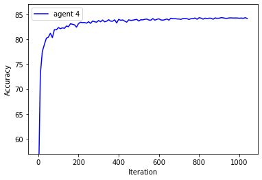
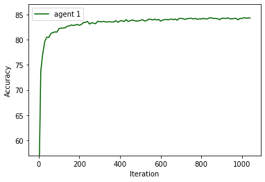
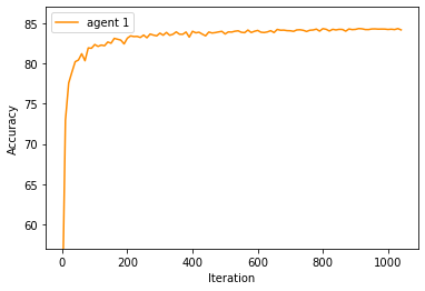
Having computed a consensus solution and weights, where we take the gradient of the potential function for each node, one can recalculate a new value for w𝑀w and compute the ROC-AUC score on test data-set, whose the size is equal to 20% of the whole data-set, for each node. The step-size constitutes diminishing step-size and is equal to α​(0)(Ξ³+t)ϕ𝛼0superscript𝛾𝑑italic-Ο•\frac{\alpha(0)}{(\gamma+t)^{\phi}}, where α​(0)𝛼0\alpha(0) = 0.008, γ𝛾\gamma = 12, Ο•italic-Ο•\phi = .45. In FigureΒ 8, we plot the ROC-AUC curve for each node in this decentralized setting. We see the convergence during one epoch (one iteration through the data). The average of nodes reaches an ROC-AUC score of 84.36% in 1000 iterations.

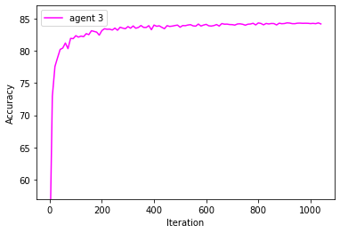
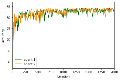
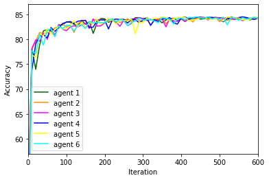
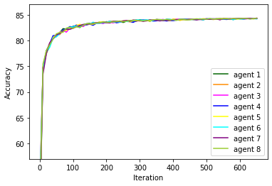
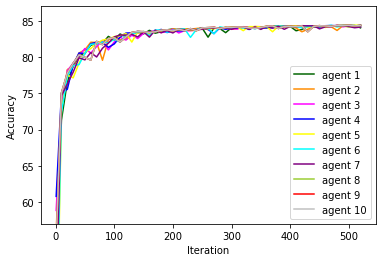
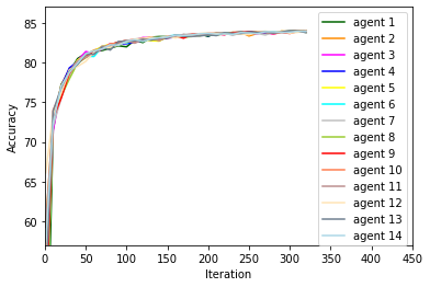
Finally, to see how the accuracy scales with the number of agents, FigureΒ 9 plots the accuracy for each agent for m∈{2,6,8,10,14}π‘š2681014m\in\{2,6,8,10,14\}. It can be observe that the cooperative sampling leads to greater stability in the overall performance, and a faster settling of the accuracy curve.
Refer to caption
(a) agent 1
Refer to caption
(b) agent 2
Refer to caption
(c) agent 3
Refer to caption
(d) agent 4
Figure 8: ROC-AUC curve in Bayesian logistic regression
Refer to caption
(a) 2 agents
Refer to caption
(b) 6 agents
Refer to caption
(c) 8 agents
Refer to caption
(d) 10 agents
Refer to caption
(e) 14 agents
Figure 9: Bayesian Logistic Regression for many agents

6 Conclusion

In this paper we considered the problem of Langevin dynamics for sampling from a distribution with a potential function consisting of data distributed across agents. We consider a decentralized framework wherein the agents communicate by the structure of a directed graph. We proved asymptotic consensus as well as convergence in Wasserstein distance to the stationary distribution of the procedure, and demonstrated the efficacy of the procedure on standard test problems in sampling.

Intended future work can be studying the properties of the method as a means of finding globally optimal points for nonconvex noisy optimization problems, as well as quantization, study of large scale speedup, and other aspects of sampling in a federated setting.

Acknowledgements

The second author would like to acknowledge support from the OP VVV project CZ.02.1.01/0.0/0.0/16_019/0000765 Research Center for Informatics

References

  • [1] ArnakΒ S Dalalyan and Avetik Karagulyan. User-friendly guarantees for the langevin monte carlo with inaccurate gradient. Stochastic Processes and their Applications, 129(12):5278–5311, 2019.
  • [2] Alain Durmus and Eric Mouline. High-dimensional bayesian inference via the unadjusted langevin algorithm. arXiv preprint arXiv: 1605.01559, 2016.
  • [3] Mert GΓΌrbΓΌzbalaban, Xuefeng Gao, Yuanhan Hu, and Lingjiong Zhu. Decentralized stochastic gradient langevin dynamics and hamiltonian monte carlo. arXiv preprint arXiv:2007.00590, 2020.
  • [4] Vyacheslav Kungurtsev. Stochastic gradient langevin dynamics on a distributed network. arXiv preprint arXiv:2001.00665, 2020.
  • [5] Daniel Levy, MatthewΒ D. Hoffman, and Jascha Sohl-Dickstein. Generalizing hamiltonian monte carlo with neural networks. arXiv preprint arXiv: 1711.09268, 2017.
  • [6] Radford M.Neal. Mcmc using hamiltonian dynamics. arXiv preprint arXiv: 1206.1901, 2012.
  • [7] Angelia Nedic. Distributed gradient methods for convex machine learning problems in networks. IEEE Signal Processing Magazine 10.1109/MSP.2020.2975210, 2018.
  • [8] Angelia Nedic and Alex Olshevsky. Distributed optimization over time-varying directed graphs. arXiv preprint arXiv: 1303.2289, 2014.
  • [9] Angelia NediΔ‡ and Alex Olshevsky. Stochastic gradient-push for strongly convex functions on time-varying directed graphs. IEEE Transactions on Automatic Control, 61(12):3936–3947, 2016.
  • [10] Angelia Nedic and Asuman Ozdaglar. Distributed subgradient methods for multi-agent optimization. IEEE Transactions on Automatic Control, 54(1):48–61, 2009.
  • [11] Kirill Neklyudov, Evgenii Egorov, Pavel Shvechnikov, and Dmitry Vetrov. Metropolis-hastings view on variational inference and adversarial training. arXiv preprint arXiv:1810.07151, 2018.
  • [12] Anjaly Parayil, HeΒ Bai, Jemin George, and Prudhvi Gurram. A decentralized approach to bayesian learning. arXiv preprint arXiv:2007.06799, 2020.
  • [13] BorisΒ T Polyak. Introduction to optimization. Number 04; QA402. 5, P6. 1987.
  • [14] Alexandr Rogozin, Cesar A.Β Uribe, Alexandr Gasnikov, Alexandr Malkovsky, and Angelia Nedic. Optimal distributed optimization on slowly time-varying graphs. arXiv preprint arXiv: 1805.06045, 2018.
  • [15] Jiaming Song, Shengjia Zhao, and Strefsefano Ermon. A-nice-mc: Adversarial training for mcmc. arXiv preprint arXiv: 1706.07561, 2017.
  • [16] MichalisΒ K. Titsias and Petros Dellaportes. Mcmc using hamiltonian dynamics. arXiv preprint arXiv: 1911.01373, 2019.
  • [17] Max Welling and YeeΒ W Teh. Bayesian learning via stochastic gradient langevin dynamics. In Proceedings of the 28th international conference on machine learning (ICML-11), pages 681–688, 2011.

7 Appendix: Proofs of Theoretical Results

Lemma 7.1.

It holds that there exists some compact set 𝒲𝒲\mathcal{W} such that for all i𝑖i

𝔼​‖X(i)​(t+1)Y(i)​(t+1)‖≀{β€–Z(i)​(t+1)β€–Z(i)​(t+1)βˆ‰π’²Rotherwise𝔼normsubscript𝑋𝑖𝑑1subscriptπ‘Œπ‘–π‘‘1casesnormsubscript𝑍𝑖𝑑1subscript𝑍𝑖𝑑1𝒲𝑅otherwise\mathbb{E}\left\|\frac{X_{(i)}(t+1)}{Y_{(i)}(t+1)}\right\|\leq\left\{\begin{array}[]{lr}\|Z_{(i)}(t+1)\|&Z_{(i)}(t+1)\notin\mathcal{W}\\ R&\text{otherwise}\end{array}\right.

with R𝑅R depending on 𝒲𝒲\mathcal{W} and problem constants.

Proof.

This is similar to the proof of Lemma 3 in Β [9].

Notice that,

X(i)​(t+1)/Y(i)​(t+1)=Z(i)​(t+1)βˆ’Ξ±β€‹(t+1)β€‹βˆ‡Ui​(Z(i)​(t+1))/Y(i)​(t+1)+α​(t+1)​B(i)​(t+1)/Y(i)​(t+1)subscript𝑋𝑖𝑑1subscriptπ‘Œπ‘–π‘‘1subscript𝑍𝑖𝑑1𝛼𝑑1βˆ‡subscriptπ‘ˆπ‘–subscript𝑍𝑖𝑑1subscriptπ‘Œπ‘–π‘‘1𝛼𝑑1subscript𝐡𝑖𝑑1subscriptπ‘Œπ‘–π‘‘1\begin{array}[]{l}X_{(i)}(t+1)/Y_{(i)}(t+1)=Z_{(i)}(t+1)-\alpha(t+1)\nabla U_{i}(Z_{(i)}(t+1))/Y_{(i)}(t+1)\\ \qquad+\sqrt{\alpha(t+1)}B_{(i)}(t+1)/Y_{(i)}(t+1)\end{array}

Without loss of generality, let X(i)′​(t+1)=X(i)​(t+1)/Y(i)​(t+1)subscriptsuperscript𝑋′𝑖𝑑1subscript𝑋𝑖𝑑1subscriptπ‘Œπ‘–π‘‘1X^{\prime}_{(i)}(t+1)=X_{(i)}(t+1)/Y_{(i)}(t+1). We know that there exists δ≀Y(i)​(t+1)≀m𝛿subscriptπ‘Œπ‘–π‘‘1π‘š\delta\leq Y_{(i)}(t+1)\leq m for all i𝑖i and t𝑑t as shown in the beginning of the proof of Theorem 2 inΒ [9].

Indeed we have, for any Z(i)​(t+1)subscript𝑍𝑖𝑑1Z_{(i)}(t+1), by strong convexity,

βˆ‡Ui​(Z(i)​(t+1))T​Z(i)​(t+1)β‰₯Ui​(Z(i)​(t+1))βˆ’Ui​(0)+ΞΌ2​‖Z(i)​(t+1)β€–2βˆ‡subscriptπ‘ˆπ‘–superscriptsubscript𝑍𝑖𝑑1𝑇subscript𝑍𝑖𝑑1subscriptπ‘ˆπ‘–subscript𝑍𝑖𝑑1subscriptπ‘ˆπ‘–0πœ‡2superscriptnormsubscript𝑍𝑖𝑑12\begin{array}[]{l}\nabla U_{i}(Z_{(i)}(t+1))^{T}Z_{(i)}(t+1)\geq U_{i}(Z_{(i)}(t+1))-U_{i}(0)\\ \qquad\qquad+\frac{\mu}{2}\|Z_{(i)}(t+1)\|^{2}\end{array}

Continuing as in the original,

β€–X(i)′​(t+1)β€–2≀(1βˆ’Ξ±β€‹(t+1)​μ/m)​‖Z(i)​(t+1)β€–2βˆ’2​α​(t+1)​(Ui​(Z(i)​(t+1))βˆ’Ui​(0))/Y(i)​(t+1)2βˆ’2​α​(t+1)​B(i)​(t+1)T​Z(i)​(t+1)/Y(i)​(t+1)2+2​α​(t+1)2β€‹β€–βˆ‡Ui​(Z(i)​(t+1))β€–2/Y(i)​(t+1)+4​α​(t+1)​‖B(i)​(t+1)β€–2/Y(i)​(t+1)2superscriptnormsuperscriptsubscript𝑋𝑖′𝑑121𝛼𝑑1πœ‡π‘šsuperscriptnormsubscript𝑍𝑖𝑑122𝛼𝑑1subscriptπ‘ˆπ‘–subscript𝑍𝑖𝑑1subscriptπ‘ˆπ‘–0subscriptπ‘Œπ‘–superscript𝑑122𝛼𝑑1subscript𝐡𝑖superscript𝑑1𝑇subscript𝑍𝑖𝑑1subscriptπ‘Œπ‘–superscript𝑑122𝛼superscript𝑑12superscriptnormβˆ‡subscriptπ‘ˆπ‘–subscript𝑍𝑖𝑑12subscriptπ‘Œπ‘–π‘‘14𝛼𝑑1superscriptnormsubscript𝐡𝑖𝑑12subscriptπ‘Œπ‘–superscript𝑑12\begin{array}[]{l}\|X_{(i)}^{\prime}(t+1)\|^{2}\leq(1-\alpha(t+1)\mu/m)\|Z_{(i)}(t+1)\|^{2}\\ \qquad-2\alpha(t+1)(U_{i}(Z_{(i)}(t+1))-U_{i}(0))/Y_{(i)}(t+1)^{2}\\ \qquad-2\sqrt{\alpha(t+1)}B_{(i)}(t+1)^{T}Z_{(i)}(t+1)/Y_{(i)}(t+1)^{2}\\ \qquad+2\alpha(t+1)^{2}\|\nabla U_{i}(Z_{(i)}(t+1))\|^{2}/Y_{(i)}(t+1)\\ \qquad+4\alpha(t+1)\|B_{(i)}(t+1)\|^{2}/Y_{(i)}(t+1)^{2}\end{array}

We have that,

β€–βˆ‡Ui​(Z(i)​(t+1))β€–2≀2​L2​‖Z(i)​(t+1)β€–2+2β€‹β€–βˆ‡Ui​(0)β€–2superscriptnormβˆ‡subscriptπ‘ˆπ‘–subscript𝑍𝑖𝑑122superscript𝐿2superscriptnormsubscript𝑍𝑖𝑑122superscriptnormβˆ‡subscriptπ‘ˆπ‘–02\|\nabla U_{i}(Z_{(i)}(t+1))\|^{2}\leq 2L^{2}\|Z_{(i)}(t+1)\|^{2}+2\|\nabla U_{i}(0)\|^{2}

and so,

β€–X(i)′​(t+1)β€–2≀(1βˆ’Ξ±β€‹(t+1)​μ/m+2​α​(t+1)​L2/Ξ΄2)​‖Z(i)​(t+1)β€–2βˆ’2​α​(t+1)​(Ui​(Z(i)​(t+1))βˆ’Ui​(0))/mβˆ’2​α​(t+1)​B(i)​(t+1)T​Z(i)​(t+1)/m+4​α​(t+1)2/Ξ΄2β€‹β€–βˆ‡Ui​(0)β€–2+4​α​(t+1)/Ξ΄2​‖B(i)​(t+1)β€–2superscriptnormsuperscriptsubscript𝑋𝑖′𝑑12absent1𝛼𝑑1πœ‡π‘š2𝛼𝑑1superscript𝐿2superscript𝛿2superscriptnormsubscript𝑍𝑖𝑑122𝛼𝑑1subscriptπ‘ˆπ‘–subscript𝑍𝑖𝑑1subscriptπ‘ˆπ‘–0π‘š2𝛼𝑑1subscript𝐡𝑖superscript𝑑1𝑇subscript𝑍𝑖𝑑1π‘š4𝛼superscript𝑑12superscript𝛿2superscriptnormβˆ‡subscriptπ‘ˆπ‘–024𝛼𝑑1superscript𝛿2superscriptnormsubscript𝐡𝑖𝑑12\begin{array}[]{l}\|X_{(i)}^{\prime}(t+1)\|^{2}\\ \qquad\leq\left(1-\alpha(t+1)\mu/m+2\alpha(t+1)L^{2}/\delta^{2}\right)\|Z_{(i)}(t+1)\|^{2}\\ \qquad\qquad-2\alpha(t+1)(U_{i}(Z_{(i)}(t+1))-U_{i}(0))/m\\ \qquad\qquad-2\sqrt{\alpha(t+1)}B_{(i)}(t+1)^{T}Z_{(i)}(t+1)/m\\ \qquad\qquad+4\alpha(t+1)^{2}/\delta^{2}\|\nabla U_{i}(0)\|^{2}\\ \qquad\qquad+4\alpha(t+1)/\delta^{2}\|B_{(i)}(t+1)\|^{2}\end{array}

Taking conditional expectations on the filtration,

𝔼​‖X(i)′​(t+1)β€–2≀(1βˆ’Ξ±β€‹(t+1)​μ/m+2​α​(t+1)​L2/Ξ΄2)​‖Z(i)​(t+1)β€–2βˆ’2​α​(t+1)/m​(Ui​(Z(i)​(t+1))βˆ’Ui​(0))+4​α​(t+1)2/Ξ΄2β€‹β€–βˆ‡Ui​(0)β€–2+4​α​(t+1)​σ2/Ξ΄2𝔼superscriptnormsuperscriptsubscript𝑋𝑖′𝑑12absent1𝛼𝑑1πœ‡π‘š2𝛼𝑑1superscript𝐿2superscript𝛿2superscriptnormsubscript𝑍𝑖𝑑122𝛼𝑑1π‘šsubscriptπ‘ˆπ‘–subscript𝑍𝑖𝑑1subscriptπ‘ˆπ‘–04𝛼superscript𝑑12superscript𝛿2superscriptnormβˆ‡subscriptπ‘ˆπ‘–024𝛼𝑑1superscript𝜎2superscript𝛿2\begin{array}[]{l}\mathbb{E}\|X_{(i)}^{\prime}(t+1)\|^{2}\\ \qquad\leq\left(1-\alpha(t+1)\mu/m+2\alpha(t+1)L^{2}/\delta^{2}\right)\|Z_{(i)}(t+1)\|^{2}\\ \qquad\qquad-2\alpha(t+1)/m(U_{i}(Z_{(i)}(t+1))-U_{i}(0))\\ \qquad\qquad+4\alpha(t+1)^{2}/\delta^{2}\|\nabla U_{i}(0)\|^{2}\\ \qquad\qquad+4\alpha(t+1)\sigma^{2}/\delta^{2}\end{array} (9)

Enforce α​(t+1)≀μ4​L2𝛼𝑑1πœ‡4superscript𝐿2\alpha(t+1)\leq\frac{\mu}{4L^{2}}. We can define the set 𝒱𝒱\mathcal{V} to be such that,

𝒱:={z|Ui​(z)≀Ui​(0)+2​μL2β€‹β€–βˆ‡Ui​(0)β€–2+2​σ2}assign𝒱conditional-set𝑧subscriptπ‘ˆπ‘–π‘§subscriptπ‘ˆπ‘–02πœ‡superscript𝐿2superscriptnormβˆ‡subscriptπ‘ˆπ‘–022superscript𝜎2\mathcal{V}:=\left\{z|U_{i}(z)\leq U_{i}(0)+\frac{2\mu}{L^{2}}\|\nabla U_{i}(0)\|^{2}+2\sigma^{2}\right\}

for all i𝑖i. Since Uisubscriptπ‘ˆπ‘–U_{i} is strongly convex, this set is compact. Now clearly if Z(i)βˆ‰π’±subscript𝑍𝑖𝒱Z_{(i)}\notin\mathcal{V} then the last term inΒ (9) is negative and so by the requirement of α​(t)𝛼𝑑\alpha(t) the first term has a coefficient less than one, and so we have that 𝔼​‖X(i)′​(t+1)‖≀‖Z(i)​(t+1)‖𝔼normsuperscriptsubscript𝑋𝑖′𝑑1normsubscript𝑍𝑖𝑑1\mathbb{E}\|X_{(i)}^{\prime}(t+1)\|\leq\|Z_{(i)}(t+1)\|.

Otherwise (i.e., Z(i)​(t+1)βˆˆπ’²subscript𝑍𝑖𝑑1𝒲Z_{(i)}(t+1)\in\mathcal{W}), we have that,

𝔼​‖X(i)′​(t+1)‖≀‖Z(i)​(t+1)β€–+α​(t+1)​‖Ui​(Z(i)​(t+1))β€–/Ξ΄+α​(t+1)​σ/δ𝔼normsuperscriptsubscript𝑋𝑖′𝑑1normsubscript𝑍𝑖𝑑1𝛼𝑑1normsubscriptπ‘ˆπ‘–subscript𝑍𝑖𝑑1𝛿𝛼𝑑1πœŽπ›Ώ\begin{array}[]{l}\mathbb{E}\|X_{(i)}^{\prime}(t+1)\|\leq\|Z_{(i)}(t+1)\|+\alpha(t+1)\|U_{i}(Z_{(i)}(t+1))\|/\delta\\ \qquad\qquad\qquad+\sqrt{\alpha(t+1)}\sigma/\delta\end{array}

and the statement follows from the compactness of 𝒲𝒲\mathcal{W}.

∎

Lemma 7.2.

It holds that there exists a C𝐢C such that,

𝔼βˆ₯βˆ‡Ui(Z(i)(t+1)βˆ₯≀C\mathbb{E}\|\nabla U_{i}(Z_{(i)}(t+1)\|\leq C
Proof.

By the same argument as for Theorem 2 inΒ [9], we can conclude that 𝔼​‖Z(i)​(t+1)‖≀D<βˆžπ”Όnormsubscript𝑍𝑖𝑑1𝐷\mathbb{E}\|Z_{(i)}(t+1)\|\leq D<\infty. Indeed, we have by the same argument that 1≀Y(i)​(t)≀m1subscriptπ‘Œπ‘–π‘‘π‘š1\leq Y_{(i)}(t)\leq m, and

maxi⁑𝔼​‖Z(i)​(t+1)‖≀maxj⁑𝔼​‖X(j)​(t)Y(j)​(t)‖≀max⁑{maxi⁑‖Z(i)​(t)β€–,R}subscript𝑖𝔼normsubscript𝑍𝑖𝑑1subscript𝑗𝔼normsubscript𝑋𝑗𝑑subscriptπ‘Œπ‘—π‘‘subscript𝑖normsubscript𝑍𝑖𝑑𝑅\max_{i}\mathbb{E}\|Z_{(i)}(t+1)\|\leq\max_{j}\mathbb{E}\left\|\frac{X_{(j)}(t)}{Y_{(j)}(t)}\right\|\leq\max\left\{\max_{i}\|Z_{(i)}(t)\|,R\right\}

and the statement following from induction and iterated expectations.

Since the gradient of U​(Z(i)​(t+1))π‘ˆsubscript𝑍𝑖𝑑1U(Z_{(i)}(t+1)) is L-Lipschitz, we have,

β€–βˆ‡U​(Z(i)​(t+1))βˆ’βˆ‡U​(Xβˆ—)‖≀L​‖Z(i)​(t+1)βˆ’Xβˆ—β€–normβˆ‡π‘ˆsubscript𝑍𝑖𝑑1βˆ‡π‘ˆsuperscript𝑋𝐿normsubscript𝑍𝑖𝑑1superscript𝑋\|\nabla U(Z_{(i)(t+1)})-\nabla U(X^{*})\|\leq L\|Z_{(i)}(t+1)-X^{*}\|

where Xβˆ—superscript𝑋X^{*} is the unique global minimizer of U​(x)π‘ˆπ‘₯U(x), which exists by strong convexity. In accordance to the property of norms:

β€–aβ€–βˆ’β€–b‖≀‖aβˆ’bβ€–normπ‘Žnorm𝑏normπ‘Žπ‘\|a\|-\|b\|\leq\|a-b\|

we get,

β€–βˆ‡U​(Z(i)​(t+1))β€–βˆ’β€–βˆ‡U​(Xβˆ—)‖≀L​‖Z(i)​(t+1)βˆ’Xβˆ—β€–normβˆ‡π‘ˆsubscript𝑍𝑖𝑑1normβˆ‡π‘ˆsuperscript𝑋𝐿normsubscript𝑍𝑖𝑑1superscript𝑋\|\nabla U(Z_{(i)}(t+1))\|-\|\nabla U(X^{*})\|\leq L\|Z_{(i)}(t+1)-X^{*}\|

and

β€–βˆ‡U​(Z(i)​(t+1))‖≀L​‖Z(i)​(t+1)βˆ’Xβˆ—β€–+β€–βˆ‡U(i)​(Xβˆ—)β€–normβˆ‡π‘ˆsubscript𝑍𝑖𝑑1𝐿normsubscript𝑍𝑖𝑑1superscript𝑋normβˆ‡subscriptπ‘ˆπ‘–superscript𝑋\|\nabla U(Z_{(i)}(t+1))\|\leq L\|Z_{(i)}(t+1)-X^{*}\|+\|\nabla U_{(i)}(X^{*})\|

Hence:

π”Όβ€‹β€–βˆ‡U(i)​(Z(i)​(t+1))‖≀L​𝔼​‖Z(i)​(t+1)βˆ’Xβˆ—β€–+β€–βˆ‡U(i)​(Xβˆ—)‖𝔼normβˆ‡subscriptπ‘ˆπ‘–subscript𝑍𝑖𝑑1𝐿𝔼normsubscript𝑍𝑖𝑑1superscript𝑋normβˆ‡subscriptπ‘ˆπ‘–superscript𝑋\mathbb{E}\|\nabla U_{(i)}(Z_{(i)}(t+1))\|\leq L\mathbb{E}\|Z_{(i)}(t+1)-X^{*}\|+\|\nabla U_{(i)}(X^{*})\|

Since the gradient of U​(Xβˆ—)π‘ˆsuperscript𝑋U(X^{*}) equals zero, then one can show 𝔼​‖Z(i)​(t+1)βˆ’Xβˆ—β€–π”Όnormsubscript𝑍𝑖𝑑1superscript𝑋\mathbb{E}\|Z_{(i)}(t+1)-X^{*}\| is bounded, and the reverse triangle inequality implies the final result.

∎

This is the same as Corollary 1 in Β [9],

Lemma 7.3.

It holds that,

β€–Z(i)​(t+1)βˆ’βˆ‘i=1mX(i)​(t)m‖≀8δ​(Ξ»tβ€‹βˆ‘i=1mβ€–X(i)​(0)β€–1+βˆ‘s=1tΞ»tβˆ’sβ€‹βˆ‘i=1mβ€–ei​(s)β€–)normsubscript𝑍𝑖𝑑1superscriptsubscript𝑖1π‘šsubscriptπ‘‹π‘–π‘‘π‘šabsent8𝛿superscriptπœ†π‘‘superscriptsubscript𝑖1π‘šsubscriptnormsubscript𝑋𝑖01superscriptsubscript𝑠1𝑑superscriptπœ†π‘‘π‘ superscriptsubscript𝑖1π‘šnormsubscript𝑒𝑖𝑠\begin{array}[]{l}\left\|Z_{(i)}(t+1)-\frac{\sum\limits_{i=1}^{m}X_{(i)}(t)}{m}\right\|\\ \qquad\leq\frac{8}{\delta}\left(\lambda^{t}\sum\limits_{i=1}^{m}\|X_{(i)}(0)\|_{1}+\sum\limits_{s=1}^{t}\lambda^{t-s}\sum\limits_{i=1}^{m}\left\|e_{i}(s)\right\|\right)\end{array}

where,

ei(s)=Ξ±(s+1)βˆ‡U(i)(Z(i)(s+1)))+2​α​(s+1)B(s+1)(i)e_{i}(s)=\alpha(s+1)\nabla U_{(i)}(Z_{(i)}(s+1)))+\sqrt{2\alpha(s+1)}B(s+1)_{(i)}
Proof.

The proof of the lemma is a direct analog of the proof Lemma 1 in  [8]. ∎

Lemma 7.4.
𝔼​[βˆ‘t=1Ο„β€–Z(i)​(t+1)βˆ’βˆ‘i=1mX(i)​(t)mβ€–]≀8δ​λ1βˆ’Ξ»β€‹βˆ‘i=1mβ€–X(i)​(0)β€–1+8δ​D​m1βˆ’Ξ»β€‹(1+Ο„)𝔼delimited-[]superscriptsubscript𝑑1𝜏normsubscript𝑍𝑖𝑑1superscriptsubscript𝑖1π‘šsubscriptπ‘‹π‘–π‘‘π‘šabsent8π›Ώπœ†1πœ†superscriptsubscript𝑖1π‘šsubscriptnormsubscript𝑋𝑖018π›Ώπ·π‘š1πœ†1𝜏\begin{array}[]{l}\mathbb{E}\left[\sum\limits_{t=1}^{\tau}\left\|Z_{(i)}(t+1)-\frac{\sum\limits_{i=1}^{m}X_{(i)}(t)}{m}\right\|\right]\\ \qquad\leq\frac{8}{\delta}\frac{\lambda}{1-\lambda}\sum\limits_{i=1}^{m}\|X_{(i)}(0)\|_{1}+\frac{8}{\delta}\frac{Dm}{1-\lambda}(1+\sqrt{\tau})\end{array}
Proof.

The proof of this result is the same as Corollary 2 in Β [9]. Note that because of the square root of α𝛼\alpha term in the noise, we integrate out 1/t1𝑑1/\sqrt{t} instead of 1/t1𝑑1/t, hence the Ο„πœ\sqrt{\tau} instead of logβ‘Ο„πœ\log\tau here. ∎

Now define,

X¯​(t)=βˆ‘i=1mX(i)​(t)m¯𝑋𝑑superscriptsubscript𝑖1π‘šsubscriptπ‘‹π‘–π‘‘π‘š\bar{X}(t)=\frac{\sum\limits_{i=1}^{m}X_{(i)}(t)}{m}
Lemma 7.5.

We have, by the column-stochasticity of A​(t)𝐴𝑑A(t),

X¯​(t+1)=X¯​(t)βˆ’Ξ±β€‹(t+1)mβ€‹βˆ‘i=1mβˆ‡U​(X¯​(t))+α​(t+1)mβ€‹βˆ‘i=1m(βˆ‡U​(X¯​(t))βˆ’U​(Z(i)​(t+1)))+B¯​(t+1)¯𝑋𝑑1¯𝑋𝑑𝛼𝑑1π‘šsuperscriptsubscript𝑖1π‘šβˆ‡π‘ˆΒ―π‘‹π‘‘π›Όπ‘‘1π‘šsuperscriptsubscript𝑖1π‘šβˆ‡π‘ˆΒ―π‘‹π‘‘π‘ˆsubscript𝑍𝑖𝑑1¯𝐡𝑑1\begin{array}[]{l}\bar{X}(t+1)=\bar{X}(t)-\frac{\alpha(t+1)}{m}\sum\limits_{i=1}^{m}\nabla U(\bar{X}(t))\\ \qquad+\frac{\alpha(t+1)}{m}\sum\limits_{i=1}^{m}\left(\nabla U(\bar{X}(t))-U(Z_{(i)}(t+1))\right)+\bar{B}(t+1)\end{array} (10)
Proof.

In accordance with the algorithm one can rewrite the final equation system as follows:

X(i)​(t+1)=|A​(t)​X​(t)|(i)βˆ’Ξ±β€‹(t+1)β€‹βˆ‡U(i)​(Z(i)​(t+1))+B(i)​(t+1)subscript𝑋𝑖𝑑1subscript𝐴𝑑𝑋𝑑𝑖𝛼𝑑1βˆ‡subscriptπ‘ˆπ‘–subscript𝑍𝑖𝑑1subscript𝐡𝑖𝑑1X_{(i)}(t+1)=|A(t)X(t)|_{(i)}-\alpha(t+1)\nabla U_{(i)}(Z_{(i)}(t+1))+B_{(i)}(t+1)

Then, one can average a column-vector that is composed of such X(i)subscript𝑋𝑖X_{(i)}, where i∈{1,..,m}i\in\{1,..,m\} . Then:

X¯​(t+1)=βˆ‘i=1m|A​(t)​X​(t)m|(i)βˆ’Ξ±β€‹(t+1)mβ€‹βˆ‘i=1mβˆ‡U(i)​(Z(i)​(t+1))+B¯​(t+1)¯𝑋𝑑1superscriptsubscript𝑖1π‘šsubscriptπ΄π‘‘π‘‹π‘‘π‘šπ‘–π›Όπ‘‘1π‘šsuperscriptsubscript𝑖1π‘šβˆ‡subscriptπ‘ˆπ‘–subscript𝑍𝑖𝑑1¯𝐡𝑑1\begin{array}[]{l}\overline{X}(t+1)=\sum_{i=1}^{m}\left|\frac{A(t)X(t)}{m}\right|_{(i)}-\frac{\alpha(t+1)}{m}\sum_{i=1}^{m}\nabla U_{(i)}(Z_{(i)}(t+1))\\ \qquad\qquad\qquad+\overline{B}(t+1)\end{array}

Having recalled A is a column-stochastic matrix, then :

1T​u=1T​A​(t)​usuperscript1𝑇𝑒superscript1𝑇𝐴𝑑𝑒1^{T}u=1^{T}A(t)u

for any vector u𝑒u. Then:

1mβ€‹βˆ‘i=1m|1​A​(t)​X​(t)|(i)=1mβ€‹βˆ‘i=1mX(i)=X¯​(t)1π‘šsuperscriptsubscript𝑖1π‘šsubscript1𝐴𝑑𝑋𝑑𝑖1π‘šsuperscriptsubscript𝑖1π‘šsubscript𝑋𝑖¯𝑋𝑑\frac{1}{m}\sum_{i=1}^{m}|1A(t)X(t)|_{(i)}=\frac{1}{m}\sum_{i=1}^{m}X_{(i)}=\overline{X}(t)

Then, one can rewrite the scheme as follow:

X¯​(t+1)=X¯​(t)βˆ’Ξ±β€‹(t+1)mβ€‹βˆ‘i=1mβˆ‡U(i)​(Z(i)​(t+1))+B¯​(t+1)¯𝑋𝑑1¯𝑋𝑑𝛼𝑑1π‘šsuperscriptsubscript𝑖1π‘šβˆ‡subscriptπ‘ˆπ‘–subscript𝑍𝑖𝑑1¯𝐡𝑑1\overline{X}(t+1)=\overline{X}(t)-\frac{\alpha(t+1)}{m}\sum_{i=1}^{m}\nabla U_{(i)}(Z_{(i)}(t+1))+\overline{B}(t+1)

Adding and subtracting α​(t+1)mβ€‹βˆ‘i=1mβˆ‡U​(X¯​(t))𝛼𝑑1π‘šsuperscriptsubscript𝑖1π‘šβˆ‡π‘ˆΒ―π‘‹π‘‘\frac{\alpha(t+1)}{m}\sum_{i=1}^{m}\nabla U(\overline{X}(t)), we get the desired expression. ∎

We have the following Corollary,

Corollary 7.5.1.

Given any Ξ³>0𝛾0\gamma>0, there exists C𝐢C positive such that,

Eβˆ₯XΒ―(t))βˆ’Z(i)(t+1)βˆ₯≀Ct1/2βˆ’Ξ³E\|\bar{X}(t))-Z_{(i)}(t+1)\|\leq\frac{C}{t^{1/2-\gamma}}

We are now ready to use the arguments in Β [1] regarding a perturbed Langevin methods. In particular, we can apply Proposition 2 to state that,

Lemma 7.6.
W2​(Ξ½Β―t+1,Ο€)≀ρt+1​W2​(Ξ½t,Ο€)+1.65​L​(Ξ±t+13​d)1/2+Ξ±(t+1)dLβˆ‘i=1m𝔼βˆ₯XΒ―(t))βˆ’Z(i)(t+1)βˆ₯\begin{array}[]{l}W_{2}(\bar{\nu}_{t+1},\pi)\leq\rho_{t+1}W_{2}(\nu_{t},\pi)+1.65L(\alpha_{t+1}^{3}d)^{1/2}\\ \qquad+\alpha(t+1)\sqrt{d}L\sum\limits_{i=1}^{m}\mathbb{E}\|\bar{X}(t))-Z_{(i)}(t+1)\|\end{array}

where ρt+1=max⁑(1βˆ’ΞΌβ€‹Ξ±β€‹(t+1),L​α​(t+1)βˆ’1)subscriptπœŒπ‘‘11πœ‡π›Όπ‘‘1𝐿𝛼𝑑11\rho_{t+1}=\max(1-\mu\alpha(t+1),L\alpha(t+1)-1).

Now recall

Lemma 7.7.

[13, Lemma 2.4] Let ukβ‰₯0subscriptπ‘’π‘˜0u_{k}\geq 0 and,

uk+1≀(1βˆ’ck)​uk+dkp+1subscriptπ‘’π‘˜11π‘π‘˜subscriptπ‘’π‘˜π‘‘superscriptπ‘˜π‘1u_{k+1}\leq\left(1-\frac{c}{k}\right)u_{k}+\frac{d}{k^{p+1}}

with d>0𝑑0d>0, p>0𝑝0p>0 and c>0𝑐0c>0 and c>p𝑐𝑝c>p. Then,

uk≀d​(cβˆ’p)βˆ’1​kβˆ’p+o​(kβˆ’p)subscriptπ‘’π‘˜π‘‘superscript𝑐𝑝1superscriptπ‘˜π‘π‘œsuperscriptπ‘˜π‘u_{k}\leq d(c-p)^{-1}k^{-p}+o(k^{-p})

Apply the previous two Lemmas together with CorollaryΒ 4.4.1 to conclude,

Theorem 7.8.

Let α​(0)≀min⁑{12​L,ΞΌ4​L2}𝛼012πΏπœ‡4superscript𝐿2\alpha(0)\leq\min\left\{\frac{1}{2L},\frac{\mu}{4L^{2}}\right\} and α​(t)=α​(0)/(1+t)𝛼𝑑𝛼01𝑑\alpha(t)=\alpha(0)/(1+t). We have that,

W2​(Ξ½Β―k+1,Ο€)≀(Cγ​m+1.65)​L​d1/2(μ​α​(0)βˆ’1/2+Ξ³)​(1+t)(1/2βˆ’Ξ³)+Ξ²ksubscriptπ‘Š2subscriptΒ―πœˆπ‘˜1πœ‹subscriptπΆπ›Ύπ‘š1.65𝐿superscript𝑑12πœ‡π›Ό012𝛾superscript1𝑑12𝛾subscriptπ›½π‘˜W_{2}(\bar{\nu}_{k+1},\pi)\leq\frac{(C_{\gamma}m+1.65)Ld^{1/2}}{(\mu\alpha(0)-1/2+\gamma)(1+t)^{(1/2-\gamma)}}+\beta_{k}

where Ξ²k=o​((1+t)βˆ’(1/2βˆ’Ξ³))subscriptπ›½π‘˜π‘œsuperscript1𝑑12𝛾\beta_{k}=o\left((1+t)^{-(1/2-\gamma)}\right)