Rigidity of discrete conformal structures on surfaces

Abstract.

In [10], Glickenstein introduced the discrete conformal structures on polyhedral surfaces in an axiomatic approach from Riemannian geometry perspective. Glickenstein’s discrete conformal structures include Thurston’s circle packings, Bowers-Stephenson’s inversive distance circle packings and Luo’s vertex scalings as special cases. Glickenstein [11] further conjectured the rigidity of the discrete conformal structures on polyhedral surfaces. Glickenstein’s conjecture includes Luo’s conjecture on the rigidity of vertex scalings [24] and Bowers-Stephenson’s conjecture on the rigidity of inversive distance circle packings [3] as special cases. In this paper, we prove Glickenstein’s conjecture using variational principles. This unifies and generalizes the well-known results of Luo [25] and Bobenko-Pinkall-Springborn [1]. Our method provides a unified approach to similar problems. We further discuss the relationships of Glickenstein’s discrete conformal structures on polyhedral surfaces and $3$-dimensional hyperbolic geometry. As a result, we obtain some new results on the convexities of the co-volume functions of some generalized $3$-dimensional hyperbolic tetrahedra.

1. Introduction

Discrete conformal structure on polyhedral manifolds is a discrete analogue of the conformal structure on Riemannian manifolds, which assigns the discrete metrics by scalar functions defined on the vertices. Since the work of Thurston [35], there have been lots of researches on different types of discrete conformal structures on polyhedral surfaces, including the tangential circle packings, Thurston’s circle packings, Bowers-Stephenson’s inversive distance circle packings, Luo’s vertex scalings and others. Most of these discrete conformal structures were invented and studied individually in the literature. In [10], Glickenstein developed an axiomatic approach to the Euclidean discrete conformal structures on polyhedral surfaces from Riemannian geometry perspective. Following Glickenstein’s original work [10], Glickenstein-Thomas [13] introduced the hyperbolic and spherical discrete conformal structures on polyhedral surfaces in an axiomatic approach. Glickenstein-Thomas [13] further studied the classification of Glickenstein’s discrete conformal structures on polyhedral surfaces. See also Xu-Zheng [43] for a complete classification of Glickenstein’s discrete conformal structures. According to the classification, Glickenstein’s discrete conformal structures include different types of circle packings and Luo’s vertex scalings on polyhedral surfaces as special cases and generalize them to a very general context. In this paper, we study the rigidity of Glickenstein’s discrete conformal structures on closed polyhedral surfaces. In [41], we study the deformation of Glickenstein’s discrete conformal structures on surfaces.

1.1. Polyhedral surfaces, discrete conformal structures and the rigidity results

Suppose $(M,\mathcal{T})$ is a connected closed triangulated surface with a triangulation $\mathcal{T}$, which is the quotient of a finite disjoint union of triangles by identifying all the edges of triangles in pair by homeomorphisms. We use $V,E,F$ to denote the set of vertices, unoriented edges and faces in $\mathcal{T}$ respectively. For simplicity, we use one index to denote a vertex (such as $i\in V$), two indices to denote an edge (such as $\{ij\}\in E$) and three indices to denote a triangle (such as $\{ijk\}\in F$). We further use $f_{i}=f(i)$ for a function $f:V\rightarrow\mathbb{R}$, $f_{ij}=f(\{ij\})$ for a function $f:E\rightarrow\mathbb{R}$, and $f_{ijk}=f(\{ijk\})$ for a function $f:F\rightarrow\mathbb{R}$ for simplicity. Denote the set of positive real numbers as $\mathbb{R}_{>0}$ and $|V|=N$.

Definition 1.1 ([26]).

A polyhedral surface $(M,\mathcal{T},l)$ with background geometry $\mathbb{G}$ ($\mathbb{G}=\mathbb{E}^{2},\mathbb{H}^{2}$ or $\mathbb{S}^{2}$) is a triangulated surface $(M,\mathcal{T})$ with a map $l:E\rightarrow\mathbb{R}_{>0}$ such that any face $\{ijk\}\in F$ can be embedded in $\mathbb{G}$ as a nondegenerate triangle with edge lengths $l_{ij},l_{ik},l_{jk}$ given by $l$. We call $l:E\rightarrow\mathbb{R}_{>0}$ as a Euclidean (hyperbolic or spherical respectively) polyhedral metric if $\mathbb{G}=\mathbb{E}^{2}$ ($\mathbb{G}=\mathbb{H}^{2}$ or $\mathbb{G}=\mathbb{S}^{2}$ respectively).

The nondegenerate condition for the face $\{ijk\}\in F$ in Definition 1.1 is equivalent to the edge lengths $l_{ij},l_{ik},l_{jk}$ satisfy the triangle inequalities ($l_{ij}+l_{ik}+l_{jk}<2\pi$ additionally if $\mathbb{G}=\mathbb{S}^{2}$). Intuitively, a polyhedral surface with background geometry $\mathbb{G}$ ($\mathbb{G}=\mathbb{E}^{2},\mathbb{H}^{2}$ or $\mathbb{S}^{2}$) can be obtained by gluing triangles in $\mathbb{G}$ isometrically along the edges in pair. For polyhedral surfaces, there may exist conic singularities at the vertices, which can be described by combinatorial curvatures. The combinatorial curvature is a map $K:V\rightarrow(-\infty,2\pi)$ that assigns the vertex $i\in V$ $2\pi$ less the sum of inner angles at $i$, i.e.

(1) $$K_{i}=2\pi-\sum_{\{ijk\}\in F}\theta_{i}^{jk},$$

where $\theta_{i}^{jk}$ is the inner angle at $i$ in the triangle $\{ijk\}$.

Definition 1.2 ([10, 13]).

Suppose $(M,\mathcal{T})$ is a triangulated connected closed surface and $\varepsilon:V\rightarrow\{-1,0,1\}$, $\eta:E\rightarrow\mathbb{R}$ are two weights defined on the vertices and edges respectively. A discrete conformal structure on the weighted triangulated surface $(M,\mathcal{T},\varepsilon,\eta)$ with background geometry $\mathbb{G}$ is composed of the maps $f:V\rightarrow\mathbb{R}$ such that

(1):

the edge length $l_{ij}$ for the edge $\{ij\}\in E$ is given by

(2) $$l_{ij}=\sqrt{\varepsilon_{i}e^{2f_{i}}+\varepsilon_{j}e^{2f_{j}}+2\eta_{ij}e^{f_{i}+f_{j}}}$$

for $\mathbb{G}=\mathbb{E}^{2}$,

(3) $$l_{ij}=\cosh^{-1}\left(\sqrt{(1+\varepsilon_{i}e^{2f_{i}})(1+\varepsilon_{j}e^{2f_{j}})}+\eta_{ij}e^{f_{i}+f_{j}}\right)$$

for $\mathbb{G}=\mathbb{H}^{2}$ and

(4) $$l_{ij}=\cos^{-1}\left(\sqrt{(1-\varepsilon_{i}e^{2f_{i}})(1-\varepsilon_{j}e^{2f_{j}})}-\eta_{ij}e^{f_{i}+f_{j}}\right)$$

for $\mathbb{G}=\mathbb{S}^{2}$;

(2):

the edge length function $l:E\rightarrow\mathbb{R}_{>0}$ defined by (2), (3), (4) is a Euclidean, hyperbolic and spherical polyhedral metric on $(M,\mathcal{T})$ respectively.

The weights $\varepsilon:V\rightarrow\{-1,0,1\}$ and $\eta:E\rightarrow\mathbb{R}$ are called the scheme coefficient and discrete conformal coefficient respectively. A function $f:V\rightarrow\mathbb{R}$ is called a discrete conformal factor and a function $f:V\rightarrow\mathbb{R}$ with the induced edge length function $l:E\rightarrow\mathbb{R}_{>0}$ being a polyhedral metric is called a nondegenerate discrete conformal factor.

Remark 1.3.

It is a remarkable result of Glickenstein-Thomas [13] that Glickenstein’s discrete conformal structure can be classified, which has the form given in Definition 1.2 with $\varepsilon_{i}\in\{-1,0,1\}$ replaced by a constant $\alpha_{i}\in\mathbb{R}$. See also Xu-Zheng [43]. As pointed out by Thomas ([34] page 53), one can reparameterize Glickenstein’s discrete conformal structures so that $\alpha_{i}\in\{-1,0,1\}$ while keeping the induced polyhedral metrics invariant. This is the motivation of Definition 1.2.

Scheme	$\varepsilon_{i}$	$\varepsilon_{j}$	$\eta_{ij}$
Tangential circle packings	$+1$	$+1$	$+1$
Thurston’s circle packings	$+1$	$+1$	$(-1,1]$
Bowers-Stephenson’s inversive distance circle packings	$+1$	$+1$	$(-1,+\infty)$
Luo’s vertex scalings	$0$	$0$	$(0,+\infty)$
Glickenstein’s discrete conformal structures	$\{+1,0,-1\}$	$\{+1,0,-1\}$	$(-1,+\infty)$

Table 1. Different types of discrete conformal structures

Remark 1.4.

The relationships of Glickenstein’s discrete conformal structures in Definition 1.2 and the existing special types of discrete conformal structures are contained in Table 1. By Table 1, the tangential circle packing is a special case of Thurston’s circle packing and Thurston’s circle packing is a special case of Bowers-Stephenson’s inversive distance circle packing. For simplicity, we unify all these three types of circle packings as inversive distance circle packings in the following. By Table 1 again, Glickenstein’s discrete conformal structures in Definition 1.2 include Bowers-Stephenson’s inversive distance circle packings and Luo’s vertex scalings as special cases. Furthermore, Glickenstein’s discrete conformal structures in Definition 1.2 include the mixed type discrete conformal structures. Specially, it contains the type with $\varepsilon_{i}=0$ for some vertices $i\in V$ and $\varepsilon_{j}=1$ for the other vertices $j\in V$. The geometry of such mixed type discrete conformal structures is seldom studied in the literature.

A basic problem in discrete conformal geometry is to understand the relationships between the discrete conformal factors and their combinatorial curvatures. We prove the following result on the rigidity of Glickenstein’s discrete conformal structures on polyhedral surfaces.

Theorem 1.5.

Suppose $(M,\mathcal{T},\varepsilon,\eta)$ is a weighted triangulated connected closed surface with the weights $\varepsilon:V\rightarrow\{0,1\}$ and $\eta:E\rightarrow\mathbb{R}$ satisfying the structure conditions

(5) $$\varepsilon_{s}\varepsilon_{t}+\eta_{st}>0,\ \ \forall\{st\}\in E$$

and

(6) $$\varepsilon_{q}\eta_{st}+\eta_{qs}\eta_{qt}\geq 0,\ \ \{q,s,t\}=\{i,j,k\}$$

for any triangle $\{ijk\}\in F$.

(a):

A nondegenerate Euclidean discrete conformal factor $f:V\rightarrow\mathbb{R}$ on $(M,\mathcal{T},\varepsilon,\eta)$ is determined by its combinatorial curvature $K:V\rightarrow\mathbb{R}$ up to a vector $c(1,1,\cdots,1),c\in\mathbb{R}$.

(b):

A nondegenerate hyperbolic discrete conformal factor $f:V\rightarrow\mathbb{R}$ on $(M,\mathcal{T},\varepsilon,\eta)$ is determined by its combinatorial curvature $K:V\rightarrow\mathbb{R}$.

Remark 1.6.

Theorem 1.5 confirms a conjecture of Glickenstein in [11]. If $\varepsilon\equiv 1$, Theorem 1.5 is reduced to the rigidity of Bowers-Stephenson’s inversive distance circle packings on surfaces obtained by Guo [17], Luo [25] and the author [39, 40], which was conjectured by Bowers-Stephenson [3]. If $\varepsilon\equiv 0$, Theorem 1.5 is reduced to the rigidity of Luo’s vertex scalings on surfaces obtained by Luo [24] and Bobenko-Pinkall-Springborn [1], the global rigidity of which was conjectured by Luo [24]. Theorem 1.5 unifies these rigidity results. Furthermore, Theorem 1.5 includes the rigidity of the mixed type discrete conformal structures, for which $\varepsilon_{i}=1$ for some vertices $i\in V_{1}\neq\emptyset$ and $\varepsilon_{j}=0$ for the other vertices $j\in V\setminus V_{1}\neq\emptyset$. The local rigidity of Glickenstein’s discrete conformal structures on polyhedral surfaces was first proved by Glickenstein [10] and Glickenstein-Thomas [13] under a condition that the discrete conformal structures induce a well-centered geometric center for each triangle in the triangulation. The local rigidity for some subcases of Glickenstein’s discrete conformal structures was also proved by Guo-Luo [18]. Theorem 1.5 includes these results on local rigidity as special cases.

1.2. Relationships with $3$-dimensional hyperbolic geometry

Motivated by Bobenko-Pinkall-Springborn’s observations [1] on the deep relationships of Luo’s vertex scalings on polyhedral surfaces and $3$-dimensional hyperbolic geometry, Zhang-Guo-Zeng-Luo-Yau-Gu [44] constructed Glickenstein’s discrete conformal structures via generalized $3$-dimensional hyperbolic tetrahedra. The basic strategy is to construct a generalized hyperbolic tetrahedron $T_{Oijk}$ with the vertices $O,v_{i},v_{j},v_{k}$ in $\mathbb{H}^{3}$, ideal or hyper-ideal. And then the discrete conformality naturally appears at some vertex triangle. In this paper, we focus on the case that the vertices are ideal or hyper-ideal. The vertex $O$ is ideal when we study Glickenstein’s Euclidean discrete conformal structures, and hyper-ideal when we study Glickenstein’s hyperbolic discrete conformal structures. The vertex $v_{s}\in\{v_{i},v_{j},v_{k}\}$ is hyper-ideal if $\varepsilon_{s}=1$, and ideal if $\varepsilon_{s}=0$. In the case that $v_{s}\in\{v_{i},v_{j},v_{k}\}$ is hyper-ideal, the line segment $Ov_{s}$ is required to have nonempty intersection with $\mathbb{H}^{3}$ in the Klein model. For each pair $\{v_{s},v_{t}\}\subseteq\{v_{i},v_{j},v_{k}\}$, a weight $\eta_{st}$ can be naturally assigned via the signed edge length of $\{v_{s}v_{t}\}$. In the Euclidean background geometry, the edge lengths of the vertex triangle $T_{Oijk}\cap H_{O}$ is given by (2), where $H_{O}$ is the horosphere attached to the ideal vertex $O$ and $f_{s}$ is minus of the signed decorated edge length $l_{Ov_{s}}$ with $s\in\{i,j,k\}$. The case for hyperbolic background geometry is similar. By truncating the generalized hyperbolic tetrahedron $T_{Oijk}$ with hyperbolic planes dual to the hyper-ideal vertices, we can attach it with a generalized hyperbolic polyhedron $P$ with finite volume. For the details on the construction of $T_{Oijk}$ and assignments of $\eta_{ij},\eta_{ik},\eta_{jk}$, please refer to Section 4.

Theorem 1.7.

Suppose $T=\{Oijk\}$ is a generalized tetrahedron constructed above.

(a):

The weights $\eta_{ij},\eta_{ik},\eta_{jk}$ on the edges $\{ij\},\{ik\},\{jk\}$ satisfy the structure conditions (5) and (6).

(b):

The co-volume of the generalized tetrahedron $T=\{Oijk\}$ defined by (83) with fixed weights $\eta_{ij},\eta_{ik},\eta_{jk}$ is a convex function of the signed edge lengths $l_{Ov_{i}},l_{Ov_{j}},l_{Ov_{k}}$.

1.3. Basic ideas of the proof of Theorem 1.5

The proof for the rigidity of Glickenstein’s discrete conformal structures on triangulated surfaces, i.e. Theorem 1.5, involves a variational principle introduced by Colin de Verdière [7]. The variational principle has been extensively studied in [1, 2, 5, 6, 17, 18, 23, 24, 25, 26, 30, 33] and others. Glickenstein [10] and Glickenstein-Thomas [13] generalized the variational principle to Glickenstein’s discrete conformal structures and proved some results on the local rigidity of Glickenstein’s discrete conformal structures. In this paper, we use Glickenstein’s variational principle to prove the local and global rigidity of Glickenstein’s discrete conformal structures. The key ingredient using Glickenstein’s variational principle to prove the rigidity is constructing a globally defined convex function with the combinatorial curvature as its gradient. This can be reduced to constructing a globally defined concave function of the discrete conformal factors on a triangle with the inner angles as its gradient. The main difficulties come from the characterization of the admissible space of nondegenerate discrete conformal factors on a triangle and the local concavity of the function with the inner angles as its gradient. We construct such a function in three steps. In the first step, we give an analytical characterization of the admissible space of nondegenerate discrete conformal factors on a triangle. This is accomplished by solving the global triangle inequalities with the help of the geometric center introduced by Glickenstein [10, 12]. As a result, the admissible space of nondegenerate discrete conformal factors on a triangle is proved to be homotopy equivalent to $\mathbb{R}^{3}$ and hence simply connected. This implies that the Ricci energy function, defined as the integral of the inner angles on the admissible space of nondegenerate discrete conformal factors for a triangle, is well-defined. In the second step, we show that the Ricci energy function for a triangle is locally concave. To achieve this, we introduce the parameterized admissible space of the nondegenerate discrete conformal factors, and choose some good point in the space such that the hession matrix of the Ricci energy function is negative definite at this point. By the continuity of the eigenvalues of the hession matrix, we prove the local concavity of the Ricci energy function. In the final step, we extend the locally concave Ricci energy function defined on the admissible space of nondegenerate discrete conformal factors for a triangle to be a globally defined concave function. The extension is now standard since Bobenko-Pinkall-Springborn’s important work [1]. In this paper, we use Luo’s generalization [25] of Bobenko-Pinkall-Springborn’s extension in [1] to extend the locally concave Ricci energy function to be a globally defined concave function.

1.4. The organization of the paper

In Section 2, we study the rigidity of Glickenstein’s Euclidean discrete conformal structures on polyhedral surfaces and prove a generalization of Theorem 1.5 (a). In Section 3, we study the rigidity of Glickenstein’s hyperbolic discrete conformal structures on polyhedral surfaces and prove a generalization of Theorem 1.5 (b). In Section 4, we discuss the relationships of Glickenstein’s discrete conformal structures on polyhedral surfaces and $3$-dimensional hyperbolic geometry and prove Theorem 1.7. In Section 5, we discuss some open problems.

Acknowledgements
The research of the author is supported by Fundamental Research Funds for the Central Universities under Grant no. 2042020kf0199.

2. Euclidean discrete conformal structures

2.1. Admissible space of nondegenerate Euclidean discrete conformal factors on a triangle

Let $\sigma=\{ijk\}$ be a triangle with the vertex set $V_{\sigma}=\{i,j,k\}$ and the edge set $E_{\sigma}=\{\{ij\},\{ik\},\{jk\}\}$. Unless otherwise declared, we use $(\{ijk\},\varepsilon,\eta)$ to denote a weighted triangle with two weights $\varepsilon:V_{\sigma}\rightarrow\{0,1\}$ and $E_{\sigma}\rightarrow\mathbb{R}$ satisfying the structure conditions (5) and (6) in the following. In the Euclidean background geometry, the lengths $l_{ij},l_{ik},l_{jk}$ of the edges in $E_{\sigma}$ are defined by the discrete conformal factor $f:V_{\sigma}\rightarrow\mathbb{R}$ via the formula (2). The discrete conformal factor $f:V_{\sigma}\rightarrow\mathbb{R}$ is nondegenerate if $l_{ij},l_{ik},l_{jk}$ satisfy the triangle inequalities, otherwise it is degenerate. We use $\Omega_{ijk}^{E}(\eta)$ to denote the space of nondegenerate Euclidean discrete conformal factors for the weighted triangle $(\{ijk\},\varepsilon,\eta)$.

Due to $\varepsilon\in\{0,1\}$ and the structure condition (5), the Cauchy inequality implies $\varepsilon_{i}e^{2f_{i}}+\varepsilon_{j}e^{2f_{j}}+2\eta_{ij}e^{f_{i}+f_{j}}\geq 2(\varepsilon_{i}\varepsilon_{j}+\eta_{ij})e^{f_{i}+f_{j}}>0$. Therefore, the Euclidean edge length $l_{ij}$ in (2) is well-defined. Note that the edge lengths $l_{ij},l_{ik},l_{jk}$ satisfy the triangle inequalities

(7) $$l_{ij}<l_{ik}+l_{jk},\ l_{ik}<l_{ij}+l_{jk},\ l_{jk}<l_{ij}+l_{ik}$$

if and only if

(8) $$0< (l_{ij}+l_{ik}+l_{jk})(l_{ij}+l_{ik}-l_{jk})(l_{ij}-l_{ik}+l_{jk})(-l_{ij}+l_{ik}+l_{jk})$$

$$= 2l_{ij}^{2}l_{ik}^{2}+2l_{ij}^{2}l_{jk}^{2}+2l_{ik}^{2}l_{jk}^{2}-l_{ij}^{4}-l_{ik}^{4}-l_{jk}^{4}.$$

For simplicity, set

(9) $$r_{i}=e^{f_{i}},\ \forall i\in V_{\sigma}.$$

Then the edge length $l_{ij}$ in the Euclidean background geometry is given by

(10) $$l_{ij}=\sqrt{\varepsilon_{i}r_{i}^{2}+\varepsilon_{j}r_{j}^{2}+2\eta_{ij}r_{i}r_{j}}.$$

The vector $r=(r_{i},r_{j},r_{k})\in\mathbb{R}^{3}_{>0}$ is called as a radius vector. Paralleling to the discrete conformal factors, a radius vector $r:V_{\sigma}\rightarrow\mathbb{R}_{>0}$ is nondegenerate if $l_{ij},l_{ik},l_{jk}$ satisfy the triangle inequalities, otherwise it is degenerate. Submitting (10) into (8) and by direct calculations, we have

(11) $$(l_{ij}+l_{ik}+l_{jk})(l_{ij}+l_{ik}-l_{jk})(l_{ij}-l_{ik}+l_{jk})(-l_{ij}+l_{ik}+l_{jk})$$

$$= 4r_{i}^{2}r_{j}^{2}r_{k}^{2}[(\varepsilon_{i}\varepsilon_{j}-\eta_{ij}^{2})r_{k}^{-2}+(\varepsilon_{i}\varepsilon_{k}-\eta_{ik}^{2})r_{j}^{-2}+(\varepsilon_{j}\varepsilon_{k}-\eta_{jk}^{2})r_{i}^{-2}$$

$$+2(\varepsilon_{k}\eta_{ij}+\eta_{ik}\eta_{jk})r_{i}^{-1}r_{j}^{-1}+2(\varepsilon_{j}\eta_{ik}+\eta_{ij}\eta_{jk})r_{i}^{-1}r_{k}^{-1}+2(\varepsilon_{i}\eta_{jk}+\eta_{ij}\eta_{ik})r_{j}^{-1}r_{k}^{-1}].$$

Set

(12) $$\kappa_{i}=r_{i}^{-1},\kappa_{j}=r_{j}^{-1},\kappa_{k}=r_{k}^{-1},$$

(13) $$\gamma_{i}=\varepsilon_{i}\eta_{jk}+\eta_{ij}\eta_{ik},\gamma_{j}=\varepsilon_{j}\eta_{ik}+\eta_{ij}\eta_{jk},\gamma_{k}=\varepsilon_{k}\eta_{ij}+\eta_{ik}\eta_{jk},$$

(14) $$Q^{E}= (\varepsilon_{j}\varepsilon_{k}-\eta_{jk}^{2})\kappa_{i}^{2}+(\varepsilon_{i}\varepsilon_{k}-\eta_{ik}^{2})\kappa_{j}^{2}+(\varepsilon_{i}\varepsilon_{j}-\eta_{ij}^{2})\kappa_{k}^{2}+2\kappa_{i}\kappa_{j}\gamma_{k}+2\kappa_{i}\kappa_{k}\gamma_{j}+2\kappa_{j}\kappa_{k}\gamma_{i}.$$

Then the structure condition (6) for the triangle $\sigma=\{ijk\}$ is equivalent to

(15) $$\gamma_{i}\geq 0,\gamma_{j}\geq 0,\gamma_{k}\geq 0$$

and the formula (11) can be written as

$$(l_{ij}+l_{ik}+l_{jk})(l_{ij}+l_{ik}-l_{jk})(l_{ij}-l_{ik}+l_{jk})(-l_{ij}+l_{ik}+l_{jk})=4r_{i}^{2}r_{j}^{2}r_{k}^{2}Q^{E}.$$

As a consequence of the arguments above, we have the following result.

Lemma 2.1.

For the weighted triangle $(\{ijk\},\varepsilon,\eta)$, the edge lengths $l_{ij},l_{ik},l_{jk}$ defined by (2) satisfy the triangle inequalities if and only if $Q^{E}>0$.

Set

(16) $$h_{i}= (\varepsilon_{j}\varepsilon_{k}-\eta_{jk}^{2})\kappa_{i}+\kappa_{j}\gamma_{k}+\kappa_{k}\gamma_{j},$$

$$h_{j}= (\varepsilon_{i}\varepsilon_{k}-\eta_{ik}^{2})\kappa_{j}+\kappa_{i}\gamma_{k}+\kappa_{k}\gamma_{i},$$

$$h_{k}= (\varepsilon_{i}\varepsilon_{j}-\eta_{ij}^{2})\kappa_{k}+\kappa_{i}\gamma_{j}+\kappa_{j}\gamma_{i}.$$

Then we have

$$Q^{E}=\kappa_{i}h_{i}+\kappa_{j}h_{j}+\kappa_{k}h_{k}.$$

By Lemma 2.1, $r=(r_{i},r_{j},r_{k})\in\mathbb{R}^{3}_{>0}$ is a degenerate radius vector for the triangle $\{ijk\}$ if and only if $Q^{E}\leq 0$. This implies that if $r=(r_{i},r_{j},r_{k})\in\mathbb{R}^{3}_{>0}$ is a degenerate radius vector, then at least one of $h_{i},h_{j},h_{k}$ is nonpositive. Furthermore, we have the following result on the signs of $h_{i},h_{j},h_{k}$.

Lemma 2.2.

If $r=(r_{i},r_{j},r_{k})\in\mathbb{R}^{3}_{>0}$ is a degenerate radius vector on the weighted triangle $(\{ijk\},\varepsilon,\eta)$, then one of $h_{i},h_{j},h_{k}$ is negative and the other two are positive.

Proof.

We separate the proof into two steps.

Step 1: For any $r=(r_{i},r_{j},r_{k})\in\mathbb{R}^{3}_{>0}$, there is no subset $\{s,t\}\subset\{i,j,k\}$ such that $h_{s}\leq 0$ and $h_{t}\leq 0$.

Suppose otherwise $h_{i}\leq 0$, $h_{j}\leq 0$. Then by the definition of $h_{i},h_{j}$ in (16), we have

(17) $$\kappa_{j}\gamma_{k}+\kappa_{k}\gamma_{j}\leq(\eta_{jk}^{2}-\varepsilon_{j}\varepsilon_{k})\kappa_{i},$$

(18) $$\kappa_{i}\gamma_{k}+\kappa_{k}\gamma_{i}\leq(\eta_{ik}^{2}-\varepsilon_{i}\varepsilon_{k})\kappa_{j}.$$

By the structure conditions (6), the inequalities (17) and (18) imply $\eta_{jk}^{2}-\varepsilon_{j}\varepsilon_{k}\geq 0$ and $\eta_{ik}^{2}-\varepsilon_{i}\varepsilon_{k}\geq 0$. By the structure conditions (5) and $\varepsilon_{i},\varepsilon_{j},\varepsilon_{k}\in\{0,1\}$, this implies

(19) $$\eta_{jk}-\varepsilon_{j}\varepsilon_{k}\geq 0,\ \eta_{ik}-\varepsilon_{i}\varepsilon_{k}\geq 0.$$

Multiplying (17) and (18) gives $(\kappa_{j}\gamma_{k}+\kappa_{k}\gamma_{j})(\kappa_{i}\gamma_{k}+\kappa_{k}\gamma_{i})\leq\kappa_{i}\kappa_{j}(\eta_{jk}^{2}-\varepsilon_{j}\varepsilon_{k})(\eta_{ik}^{2}-\varepsilon_{i}\varepsilon_{k}).$ By the structure condition (6), this implies $\kappa_{i}\kappa_{j}\gamma_{k}^{2}\leq\kappa_{i}\kappa_{j}(\eta_{jk}^{2}-\varepsilon_{j}\varepsilon_{k})(\eta_{ik}^{2}-\varepsilon_{i}\varepsilon_{k}),$ which is equivalent to

(20) $$\gamma_{k}^{2}-(\eta_{jk}^{2}-\varepsilon_{j}\varepsilon_{k})(\eta_{ik}^{2}-\varepsilon_{i}\varepsilon_{k})=-\varepsilon_{i}\varepsilon_{j}\varepsilon_{k}+\varepsilon_{k}\eta_{ij}^{2}+\varepsilon_{j}\varepsilon_{k}\eta_{ik}^{2}+\varepsilon_{i}\varepsilon_{k}\eta_{jk}^{2}+2\varepsilon_{k}\eta_{ij}\eta_{ik}\eta_{jk}\leq 0.$$

Set

$$F=-\varepsilon_{i}\varepsilon_{j}\varepsilon_{k}+\varepsilon_{k}\eta_{ij}^{2}+\varepsilon_{j}\varepsilon_{k}\eta_{ik}^{2}+\varepsilon_{i}\varepsilon_{k}\eta_{jk}^{2}+2\varepsilon_{k}\eta_{ij}\eta_{ik}\eta_{jk}.$$

Then $F\leq 0$ by (20). On the other hand, by (19), $\varepsilon_{i},\varepsilon_{j},\varepsilon_{k}\in\{0,1\}$, (5) and (6), we have

(21) $$F= \varepsilon_{k}(\varepsilon_{i}\eta_{jk}-\varepsilon_{j}\eta_{ik})^{2}+(\varepsilon_{i}\varepsilon_{j}+\eta_{ij})[2\varepsilon_{k}\eta_{ik}\eta_{jk}+\varepsilon_{k}(\eta_{ij}-\varepsilon_{i}\varepsilon_{j})]$$

$$= \varepsilon_{k}(\varepsilon_{i}\eta_{jk}-\varepsilon_{j}\eta_{ik})^{2}+(\varepsilon_{i}\varepsilon_{j}+\eta_{ij})[\varepsilon_{k}(\varepsilon_{k}\eta_{ij}+\eta_{ik}\eta_{jk})+\varepsilon_{k}(\eta_{ik}\eta_{jk}-\varepsilon_{i}\varepsilon_{j})]$$

$$= \varepsilon_{k}(\varepsilon_{i}\eta_{jk}-\varepsilon_{j}\eta_{ik})^{2}+(\varepsilon_{i}\varepsilon_{j}+\eta_{ij})[\varepsilon_{k}\gamma_{k}+\varepsilon_{k}(\eta_{ik}-\varepsilon_{i}\varepsilon_{k})(\eta_{jk}-\varepsilon_{j}\varepsilon_{k})$$

$$\ \ \ \ \ \ \ \ \ \ \ \ \ \ \ \ \ \ \ \ \ \ \ \ \ \ \ \ \ \ \ \ \ \ \ \ \ \ \ \ \ \ \ \ \ \ \ \ \ \ \ \ \ \ +\varepsilon_{i}\varepsilon_{k}(\eta_{jk}-\varepsilon_{j}\varepsilon_{k})+\varepsilon_{j}\varepsilon_{k}(\eta_{ik}-\varepsilon_{i}\varepsilon_{k})]$$

$$\geq 0.$$

Therefore, $F=0$.

In the case of $\varepsilon_{k}=0$, by the structure condition (5), we have

(22) $$\varepsilon_{i}\varepsilon_{j}+\eta_{ij}>0,\eta_{ik}>0,\eta_{jk}>0.$$

By $h_{i}\leq 0$, $h_{j}\leq 0$ and $\varepsilon_{k}=0$, we have $\eta_{ik}\eta_{jk}\kappa_{j}+\gamma_{j}\kappa_{k}\leq\eta_{jk}^{2}\kappa_{i}$ and $\eta_{ik}\eta_{jk}\kappa_{i}+\gamma_{i}\kappa_{k}\leq\eta_{ik}^{2}\kappa_{j}$. Multiplying both sides of these two inequalities gives

$$\eta_{ik}^{2}\eta_{jk}^{2}\kappa_{i}\kappa_{j}\leq(\eta_{ik}\eta_{jk}\kappa_{j}+\gamma_{j}\kappa_{k})(\eta_{ik}\eta_{jk}\kappa_{i}+\gamma_{i}\kappa_{k})\leq\eta_{ik}^{2}\eta_{jk}^{2}\kappa_{i}\kappa_{j}.$$

This implies

(23) $$\gamma_{i}=\varepsilon_{i}\eta_{jk}+\eta_{ij}\eta_{ik}=0,\ \gamma_{j}=\varepsilon_{j}\eta_{ik}+\eta_{ij}\eta_{jk}=0,$$

which implies $\varepsilon_{i}\varepsilon_{j}-\eta_{ij}^{2}=0$ by (22). Note that $\varepsilon_{i}\varepsilon_{j}-\eta_{ij}^{2}=(\varepsilon_{i}\varepsilon_{j}-\eta_{ij})(\varepsilon_{i}\varepsilon_{j}+\eta_{ij})$. By $\varepsilon_{i}\varepsilon_{j}+\eta_{ij}>0$ in (22), we have $\varepsilon_{i}\varepsilon_{j}-\eta_{ij}=0$. By $\varepsilon_{i}\varepsilon_{j}+\eta_{ij}>0$ in (22) again, we have $\varepsilon_{i}\varepsilon_{j}>0$. Therefore, $\varepsilon_{i}=\varepsilon_{j}=\eta_{ij}=1$. Combining this with (23) gives $\eta_{ik}+\eta_{jk}=0$. This contradicts $\eta_{ik}>0,\eta_{jk}>0$ in (22).

In the case of $\varepsilon_{k}=1$, by $F=0$ and (21), we have

(24) $$\varepsilon_{i}\eta_{jk}-\varepsilon_{j}\eta_{ik}=\eta_{ij}+\eta_{ik}\eta_{jk}=(\eta_{ik}-\varepsilon_{i})(\eta_{jk}-\varepsilon_{j})=\varepsilon_{i}(\eta_{jk}-\varepsilon_{j})=\varepsilon_{j}(\eta_{ik}-\varepsilon_{i})=0.$$

This implies $\eta_{ik}=\varepsilon_{i}$ or $\eta_{jk}=\varepsilon_{j}$. By $\varepsilon_{k}=1$ and the structure condition (5), we have

(25) $$\varepsilon_{i}\varepsilon_{j}+\eta_{ij}>0,\varepsilon_{i}+\eta_{ik}>0,\varepsilon_{j}+\eta_{jk}>0.$$

If $\eta_{ik}=\varepsilon_{i}$, (25) implies $\varepsilon_{i}=\eta_{ik}=1$. Submitting this into (24) gives $\eta_{jk}=\varepsilon_{j}$. By (25) again, we have $\varepsilon_{j}=\eta_{jk}=1$. Combining $\varepsilon_{i}=\eta_{ik}=1$, $\varepsilon_{j}=\eta_{jk}=1$ and (24), we have $\eta_{ij}+\varepsilon_{i}\varepsilon_{j}=\eta_{ij}+\eta_{ik}\eta_{jk}=0$. This contradicts (25). The same arguments also apply to the case $\eta_{jk}=\varepsilon_{j}$.

Therefore, there exists no subset $\{s,t\}\subset\{i,j,k\}$ such that $h_{s}\leq 0$ and $h_{t}\leq 0$.

Step 2: If $r=(r_{i},r_{j},r_{k})\in\mathbb{R}^{3}_{>0}$ is a degenerate radius vector for the weighted triangle $(\{ijk\},\varepsilon,\eta)$, then one of $h_{i},h_{j},h_{k}$ is negative and the other two are positive.

By Lemma 2.1, if $r=(r_{i},r_{j},r_{k})\in\mathbb{R}^{3}_{>0}$ is a degenerate radius vector, we have $Q^{E}=\kappa_{i}h_{i}+\kappa_{j}h_{j}+\kappa_{k}h_{k}\leq 0$. This implies at least one of $h_{i},h_{j},h_{k}$ is nonpositive. Without loss of generality, assume $h_{i}\leq 0$. Then the result in step 1 implies that $h_{j}>0,h_{k}>0$. If $h_{i}=0$, $h_{j}>0,h_{k}>0$, we have $Q^{E}=\kappa_{i}h_{i}+\kappa_{j}h_{j}+\kappa_{k}h_{k}>0$. This contradicts $Q^{E}\leq 0$. Therefore, $h_{i}<0$, $h_{j}>0$, $h_{k}>0$. Q.E.D.

Remark 2.3.

Lemma 2.2 has an interesting geometric explanation as follows. For a nondegenerate radius vector $r\in\mathbb{R}^{3}_{>0}$ on the weighted triangle $(\{ijk\},\varepsilon,\eta)$, there exists a geometric center $C_{ijk}$ for the triangle $\{ijk\}$ ([12], Proposition 4), which has the same power distance to the vertices $i,j,k$.

Figure 1. Signed distances of geometric center

Here the power distance of a point $p$ to the vertex $i$ is defined to be $\pi_{p}(i)=d^{2}(i,p)-\varepsilon_{i}r_{i}^{2}$, where $d(i,p)$ is the Euclidean distance between $p$ and the vertex $i$. Please refer to Figure 1 for the geometric center. Denote $h_{jk,i}$ as the signed distance of the geometric center $C_{ijk}$ to the edge $\{jk\}$, which is defined to be positive if $C_{ijk}$ is on the same side of the line determined by $\{jk\}$ as the triangle $\{ijk\}$ and negative otherwise (or zero if $C_{ijk}$ is on the line). Projections of $C_{ijk}$ to the edges $\{ij\},\{ik\},\{jk\}$ give rise to the geometric centers of these edges, which are denoted by $C_{ij},C_{ik},C_{jk}$ respectively. The signed distance $d_{ij}$ of $C_{ij}$ to the vertex $i$ is defined to be positive if $C_{ij}$ is on the same side as $j$ along the line determined by $\{ij\}$ and negative otherwise (or zero if $C_{ij}$ is the same as $i$). The signed distance $d_{ji}$ is defined similarly. Note that $d_{ij}+d_{ji}=l_{ij}$ and $d_{ij}\neq d_{ji}$ in general. For nondegenerate radius vectors, we have $h_{jk,i}=\frac{d_{ji}-d_{jk}\cos\theta_{j}}{\sin\theta_{j}},\ \ d_{ij}=\frac{\varepsilon_{i}r_{i}^{2}+\eta_{ij}r_{i}r_{j}}{l_{ij}},$ where $\theta_{j}$ is the inner angle at the vertex $j$ of the triangle $\{ijk\}$. By direct calculations, we have

(26) $$h_{jk,i}=\frac{r_{i}^{2}r_{j}^{2}r_{k}^{2}}{Al_{jk}}\kappa_{i}h_{i},$$

where $A=l_{ij}l_{ik}\sin\theta_{i}$. Lemma 2.2 implies that the geometric center $C_{ijk}$ does not lie in some region in the plane determined by the triangle as the nondegenerate radius vector tends to be degenerate. Note that $h_{i},h_{j},h_{k}$ are defined for all radius vectors in $\mathbb{R}^{3}_{>0}$, while $h_{ij,k},h_{ik,j},h_{jk,i}$ are defined only for nondegenerate radius vectors.

Now we can give an analytic characterization of the admissible space of nondegenerate Euclidean discrete conformal factors on $(\{ijk\},\varepsilon,\eta)$. The main result is as follows.

Theorem 2.4.

For the weighted triangle $(\{ijk\},\varepsilon,\eta)$, the admissible space $\Omega_{ijk}^{E}(\eta)$ of nondegenerate radius vectors is a nonempty simply connected open set whose boundary components are analytic. Furthermore,

$$\Omega_{ijk}^{E}(\eta)=\mathbb{R}^{3}_{>0}\setminus\sqcup_{\alpha\in\Lambda}V_{\alpha},$$

where $\Lambda=\{q\in\{i,j,k\}|A_{q}=\eta_{st}^{2}-\varepsilon_{s}\varepsilon_{t}>0,\{q,s,t\}=\{i,j,k\}\}$, $\sqcup_{\alpha\in\Lambda}V_{\alpha}$ is a disjoint union of $V_{\alpha}$ and $V_{\alpha}$ is a closed region in $\mathbb{R}^{3}_{>0}$ bounded by an analytic function defined on $\mathbb{R}^{2}_{>0}$ by

(27) $$V_{i}=\{(r_{i},r_{j},r_{k})\in\mathbb{R}^{3}_{>0}|\kappa_{i}\geq\frac{-B_{i}+\sqrt{\Delta_{i}}}{2A_{i}}\}=\{(r_{i},r_{j},r_{k})\in\mathbb{R}^{3}_{>0}|r_{i}\leq\frac{2A_{i}}{-B_{i}+\sqrt{\Delta_{i}}}\}.$$

To prove Theorem 2.4, we first prove the following result.

Lemma 2.5.

For the weighted triangle $(\{ijk\},\varepsilon,\eta)$, if $\varepsilon_{j}\varepsilon_{k}-\eta_{jk}^{2}\geq 0$, $\varepsilon_{i}\varepsilon_{k}-\eta_{ik}^{2}\geq 0$ and $\varepsilon_{i}\varepsilon_{j}-\eta_{ij}^{2}\geq 0$, then the admissible space $\Omega^{E}_{ijk}(\eta)$ in the parameter $r$ is $\mathbb{R}^{3}_{>0}$ and hence simply connected.

Proof.

By Lemma 2.1, we just need to prove that for any $r=(r_{i},r_{j},r_{k})\in\mathbb{R}^{3}_{>0}$, we have $Q^{E}>0$. If $\varepsilon_{j}\varepsilon_{k}-\eta_{jk}^{2}\geq 0$, $\varepsilon_{i}\varepsilon_{k}-\eta_{ik}^{2}\geq 0$ and $\varepsilon_{i}\varepsilon_{j}-\eta_{ij}^{2}\geq 0$, then we have $Q^{E}\geq 0$ by the definition (14) of $Q^{E}$ and the structure condition (6). If $Q^{E}=0$, then $\eta_{jk}^{2}=\varepsilon_{j}\varepsilon_{k},\eta_{ik}^{2}=\varepsilon_{i}\varepsilon_{k},\eta_{ij}^{2}=\varepsilon_{i}\varepsilon_{j}$. Combining this with the structure condition (5), we have $\eta_{jk}=\varepsilon_{j}\varepsilon_{k},\eta_{ik}=\varepsilon_{i}\varepsilon_{k},\eta_{ij}=\varepsilon_{i}\varepsilon_{j}$. By the structure condition (5) again, this implies $\varepsilon_{i}=\varepsilon_{j}=\varepsilon_{k}=\eta_{ij}=\eta_{ik}=\eta_{jk}=1$. As a result, we have $Q^{E}=4\kappa_{i}\kappa_{j}+4\kappa_{i}\kappa_{k}+4\kappa_{j}\kappa_{k}>0$ for any $r=(r_{i},r_{j},r_{k})\in\mathbb{R}^{3}_{>0}$. It is a contradiction. Therefore, the admissible space $\Omega^{E}_{ijk}(\eta)=\mathbb{R}^{3}_{>0}$ and hence simply connected. Q.E.D.

By Lemma 2.5, we just need to study the case that at least one of $\varepsilon_{j}\varepsilon_{k}-\eta_{jk}^{2}$, $\varepsilon_{i}\varepsilon_{k}-\eta_{ik}^{2}$, $\varepsilon_{i}\varepsilon_{j}-\eta_{ij}^{2}$ is negative. Suppose $r=(r_{i},r_{j},r_{k})\in\mathbb{R}^{3}_{>0}$ is a degenerate radius vector. Then $Q^{E}\leq 0$ by Lemma 2.1. By Lemma 2.2, one of $h_{i},h_{j},h_{k}$ is negative and the other two are positive. Without loss of generality, assume $h_{i}<0$, $h_{j}>0,h_{k}>0$ at $r$. By the definition (16) of $h_{i}$ and the structure condition (6), we have $(\eta_{jk}^{2}-\varepsilon_{j}\varepsilon_{k})\kappa_{i}>\gamma_{k}\kappa_{j}+\gamma_{j}\kappa_{k}\geq 0$. This implies $\eta_{jk}^{2}-\varepsilon_{j}\varepsilon_{k}>0$. Taking $Q^{E}$ as a quadratic function of $\kappa_{i},\kappa_{j},\kappa_{k}$. Then $Q^{E}\leq 0$ is equivalent to

(28) $$A_{i}\kappa_{i}^{2}+B_{i}\kappa_{i}+C_{i}\geq 0,$$

where

(29) $$A_{i}= \eta_{jk}^{2}-\varepsilon_{j}\varepsilon_{k}>0,$$

$$B_{i}= -2(\gamma_{k}\kappa_{j}+\gamma_{j}\kappa_{k})\leq 0,$$

$$C_{i}= (\eta_{ik}^{2}-\varepsilon_{i}\varepsilon_{k})\kappa_{j}^{2}+(\eta_{ij}^{2}-\varepsilon_{i}\varepsilon_{j})\kappa_{k}^{2}-2\kappa_{j}\kappa_{k}\gamma_{i}.$$

Lemma 2.6.

For the weighted triangle $(\{ijk\},\varepsilon,\eta)$, if $A_{i}=\eta_{jk}^{2}-\varepsilon_{j}\varepsilon_{k}>0$, then the discriminant $\Delta_{i}=B_{i}^{2}-4A_{i}C_{i}$ for (28) is positive.

Proof.

By direct calculations, we have

(30) $$\Delta_{i}=4(\varepsilon_{j}\kappa_{k}^{2}+\varepsilon_{k}\kappa_{j}^{2}+2\eta_{jk}\kappa_{j}\kappa_{k})(\varepsilon_{i}\eta_{jk}^{2}+\varepsilon_{j}\eta_{ik}^{2}+\varepsilon_{k}\eta_{ij}^{2}+2\eta_{ij}\eta_{ik}\eta_{jk}-\varepsilon_{i}\varepsilon_{j}\varepsilon_{k}).$$

By the structure condition (5) and the Cauchy inequality, we have $\varepsilon_{j}\kappa_{k}^{2}+\varepsilon_{k}\kappa_{j}^{2}+2\eta_{jk}\kappa_{j}\kappa_{k}\geq 2(\varepsilon_{j}\varepsilon_{k}+\eta_{jk})\kappa_{j}\kappa_{k}>0$. Therefore, the sign of $\Delta_{i}$ is determined by the term $\varepsilon_{i}\eta_{jk}^{2}+\varepsilon_{j}\eta_{ik}^{2}+\varepsilon_{k}\eta_{ij}^{2}+2\eta_{ij}\eta_{ik}\eta_{jk}-\varepsilon_{i}\varepsilon_{j}\varepsilon_{k}$ in (30), which is symmetric in $i,j,k$.

If one of $\varepsilon_{i},\varepsilon_{j},\varepsilon_{k}$ is zero, say $\varepsilon_{i}=0$, we have $\eta_{ij}>0$ and $\eta_{ik}>0$ by the structure condition (5). This implies $\varepsilon_{i}\eta_{jk}^{2}+\varepsilon_{j}\eta_{ik}^{2}+\varepsilon_{k}\eta_{ij}^{2}+2\eta_{ij}\eta_{ik}\eta_{jk}-\varepsilon_{i}\varepsilon_{j}\varepsilon_{k}=(\varepsilon_{j}\eta_{ik}-\varepsilon_{k}\eta_{ij})^{2}+2\eta_{ij}\eta_{ik}(\eta_{jk}+\varepsilon_{j}\varepsilon_{k})>0.$ Therefore, $\Delta_{i}>0$.

If $\varepsilon_{i}=\varepsilon_{j}=\varepsilon_{k}=1$, we have

$$\varepsilon_{i}\eta_{jk}^{2}+\varepsilon_{j}\eta_{ik}^{2}+\varepsilon_{k}\eta_{ij}^{2}+2\eta_{ij}\eta_{ik}\eta_{jk}-\varepsilon_{i}\varepsilon_{j}\varepsilon_{k}=\eta_{jk}^{2}+\eta_{ik}^{2}+\eta_{ij}^{2}+2\eta_{ij}\eta_{ik}\eta_{jk}-1.$$

The positivity of this term under the condition $A_{i}=\eta_{jk}^{2}-1>0$ has been proved in Lemma 2.3 in [40]. For completeness, we present a proof here. If $\eta_{ij}\geq 0$ and $\eta_{ik}\geq 0$, by the Cauchy inequality and the structure condition (5), we have $\eta_{jk}^{2}+\eta_{ik}^{2}+\eta_{ij}^{2}+2\eta_{ij}\eta_{ik}\eta_{jk}-1\geq 2\eta_{ij}\eta_{ik}(\eta_{jk}+1)+\eta_{jk}^{2}-1\geq\eta_{jk}^{2}-1>0$. If $\eta_{ij}<0$, then $\eta_{ij}\in(-1,0)$ by the structure condition (5). This implies $\eta_{jk}^{2}+\eta_{ik}^{2}+\eta_{ij}^{2}+2\eta_{ij}\eta_{ik}\eta_{jk}-1=(\eta_{ik}+\eta_{ij}\eta_{jk})^{2}+(\eta_{jk}^{2}-1)(1-\eta_{ij}^{2})\geq(\eta_{jk}^{2}-1)(1-\eta_{ij}^{2})>0$. The same arguments apply to $\eta_{ik}<0$. Therefore, $\Delta_{i}>0$. Q.E.D.

By the proof of Lemma 2.6, we have the following corollary.

Corollary 2.7.

For the weighted triangle $(\{ijk\},\varepsilon,\eta)$, if one of $\eta_{jk}^{2}-\varepsilon_{j}\varepsilon_{k},\eta_{ik}^{2}-\varepsilon_{i}\varepsilon_{k},\eta_{ij}^{2}-\varepsilon_{i}\varepsilon_{j}$ is positive, then the term

(31) $$G:=\varepsilon_{i}\eta_{jk}^{2}+\varepsilon_{j}\eta_{ik}^{2}+\varepsilon_{k}\eta_{ij}^{2}+2\eta_{ij}\eta_{ik}\eta_{jk}-\varepsilon_{i}\varepsilon_{j}\varepsilon_{k}$$

is positive.

Remark 2.8.

One can also take $Q^{E}$ as a quadratic function of $\kappa_{j}$ or $\kappa_{k}$ and define $\Delta_{j}$, $\Delta_{k}$ similarly. By symmetry, we have $\Delta_{j}>0$ if $\eta_{ik}^{2}-\varepsilon_{i}\varepsilon_{k}>0$ and $\Delta_{k}>0$ if $\eta_{ij}^{2}-\varepsilon_{i}\varepsilon_{j}>0$.

Proof for Theorem 2.4: We solve the admissible space of nondegenerate radius vectors for $(\{ijk\},\varepsilon,\eta)$ by giving a precise description of the space of degenerate radius vectors.

Suppose $(r_{i},r_{j},r_{k})\in\mathbb{R}^{3}_{>0}$ is a degenerate radius vector for $(\{ijk\},\varepsilon,\eta)$. By Lemma 2.1, we have $Q^{E}=\kappa_{i}h_{i}+\kappa_{j}h_{j}+\kappa_{k}h_{k}\leq 0$. By Lemma 2.2, one of $h_{i},h_{j},h_{k}$ is negative and the other two are positive. Without loss of generality, assume $h_{i}<0,h_{j}>0,h_{k}>0$. By $h_{i}<0$ and the structure condition (6), we have $A_{i}=\eta_{jk}^{2}-\varepsilon_{j}\varepsilon_{k}>0$. Taking $Q^{E}\leq 0$ as a quadratic inequality of $\kappa_{i}$. By Lemma 2.6, the solution of $Q^{E}\leq 0$, i.e. $A_{i}\kappa_{i}^{2}+B_{i}\kappa_{i}+C_{i}\geq 0$, is

$$\kappa_{i}\geq\frac{-B_{i}+\sqrt{\Delta_{i}}}{2A_{i}}\ \text{or}\ \kappa_{i}\leq\frac{-B_{i}-\sqrt{\Delta_{i}}}{2A_{i}}.$$

Note that

(32) $$2A_{i}\kappa_{i}+B_{i}=2(\eta_{jk}^{2}-\varepsilon_{j}\varepsilon_{k})\kappa_{i}-2(\gamma_{k}\kappa_{j}+\gamma_{j}\kappa_{k})=-2h_{i},$$

we have $\kappa_{i}>\frac{-B_{i}}{2A_{i}}$ by $h_{i}<0$ and $A_{i}>0$. This implies the solution $(r_{i},r_{j},r_{k})\in\mathbb{R}^{3}_{>0}$ of $Q^{E}\leq 0$ with $h_{i}<0,h_{j}>0,h_{k}>0$ is $\kappa_{i}\geq\frac{-B_{i}+\sqrt{\Delta_{i}}}{2A_{i}}$. Therefore, $\mathbb{R}^{3}_{>0}\setminus\Omega_{ijk}^{E}(\eta)\subset\cup_{\alpha\in\Lambda}V_{\alpha}$, where $\Lambda=\{q\in\{i,j,k\}|A_{q}=\eta_{st}^{2}-\varepsilon_{s}\varepsilon_{t}>0,\{q,s,t\}=\{i,j,k\}\}$, $V_{i}$ is defined by (27) and $V_{j},V_{k}$ are defined similarly.

Conversely, suppose $(r_{i},r_{j},r_{k})\in\cup_{\alpha\in\Lambda}V_{\alpha}\subseteq\mathbb{R}^{3}_{>0}$. Without loss of generality, assume $(r_{i},r_{j},r_{k})\in V_{i}$ and $A_{i}=\eta_{jk}^{2}-\varepsilon_{j}\varepsilon_{k}>0$. Then $\kappa_{i}\geq\frac{-B_{i}+\sqrt{\Delta_{i}}}{2A_{i}}$ by the definition of $V_{i}$ in (27). This is equivalent to $2A_{i}\kappa_{i}+B_{i}\geq\sqrt{\Delta_{i}}$ by $A_{i}>0$. Taking the square of both sides of this inequality gives $A_{i}\kappa_{i}^{2}+B_{i}\kappa_{i}+C_{i}\geq 0$, which is equivalent to $Q^{E}\leq 0$. Therefore, $\cup_{\alpha\in\Lambda}V_{\alpha}\subset\mathbb{R}^{3}_{>0}\setminus\Omega_{ijk}^{E}(\eta).$ In summary, we have $\cup_{\alpha\in\Lambda}V_{\alpha}=\mathbb{R}^{3}_{>0}\setminus\Omega_{ijk}^{E}(\eta)$.

To see that $V_{\alpha}\cap V_{\beta}=\emptyset$ for distinct $\alpha$ and $\beta$ in $\Lambda$, suppose otherwise there exists some $(r_{i},r_{j},r_{k})\in\mathbb{R}^{3}_{>0}$ with $(r_{i},r_{j},r_{k})\in V_{i}\cap V_{j}$. Then $A_{i}>0,A_{j}>0$. By Lemma 2.6 and Remark 2.8, this implies $\Delta_{i}>0,\Delta_{j}>0$. By $(r_{i},r_{j},r_{k})\in V_{i}$, we have $\kappa_{i}\geq\frac{-B_{i}+\sqrt{\Delta_{i}}}{2A_{i}}$. Then by $A_{i}>0$ and (32), we have $h_{i}=-\frac{1}{2}(2A_{i}\kappa_{i}+B_{i})\leq-\frac{1}{2}\sqrt{\Delta_{i}}<0$. Lemma 2.2 further implies $h_{i}<0,h_{j}>0,h_{k}>0$. The same arguments applying to $(r_{i},r_{j},r_{k})\in V_{j}$ shows that $h_{j}<0,h_{i}>0,h_{k}>0$. This is a contradiction. Therefore, $V_{\alpha}\cap V_{\beta}=\emptyset$ for $\forall\alpha,\beta\in\Lambda,\alpha\neq\beta$.

Therefore, $\Omega_{ijk}^{E}(\eta)=\mathbb{R}^{3}_{>0}\setminus\sqcup_{\alpha\in\Lambda}V_{\alpha}$. As a result, the admissible space $\Omega_{ijk}^{E}(\eta)$ is homotopy equivalent to $\mathbb{R}^{3}_{>0}$ and hence simply connected. Q.E.D.

Remark 2.9.

By the proof of Theorem 2.4, if $V_{i}$ defined by (27) is nonempty and $(r_{i},r_{j},r_{k})\in V_{i}$, we have $h_{i}<0,h_{j}>0,h_{k}>0$ at $(r_{i},r_{j},r_{k})$.

Remark 2.10.

The method of characterizing the admissible space of nondegenerate discrete conformal factors on a weighted triangle in the proof of Theorem 2.4 provides a unified approach to similar problems for other types of discrete conformal structures. See [19, 40, 42] for example. The analytical characterization of the admissible space of nondegenerate discrete conformal factors on a weighted triangle has some other applications. See [4] for example for some applications in the rigidity of infinite inversive distance circle packings on the plane and the convergence of the inversive distance circle packings.

Define

$$\Omega_{ijk}^{E}=\{(r_{i},r_{j},r_{k},\eta_{ij},\eta_{ik},\eta_{jk})\in\mathbb{R}^{3}_{>0}\times\mathbb{R}^{3}|\eta\ \text{satisfies}\ (\ref{structure condition 1}),(\ref{structure condition 2})\ \text{and }(r_{i},r_{j},r_{k})\in\Omega_{ijk}^{E}(\eta)\}.$$

We call $\Omega_{ijk}^{E}$ as the parameterized admissible space of nondegenerate radius vectors for the triangle $\{ijk\}$. The parameterized admissible space $\Omega_{ijk}^{E}$ contains some points with good properties.

Lemma 2.11.

The point $(r_{i},r_{j},r_{k},\eta_{ij},\eta_{ik},\eta_{jk})=(1,1,1,1,1,1)$ is contained in $\Omega_{ijk}^{E}$. Furthermore, $h_{i}>0,h_{j}>0,h_{k}>0$ at this point.

Proof.

As $\varepsilon_{i},\varepsilon_{j},\varepsilon_{k}\in\{0,1\}$, it is straight forward to check that $(\eta_{ij},\eta_{ik},\eta_{jk})=(1,1,1)$ satisfies the structure conditions (5) and (6). By $\varepsilon_{i},\varepsilon_{j},\varepsilon_{k}\in\{0,1\}$ and the definition (16) of $h_{i},h_{j},h_{k}$, we have

$$h_{i}= (\varepsilon_{j}\varepsilon_{k}-\eta_{jk}^{2})\kappa_{i}+\kappa_{j}\gamma_{k}+\kappa_{k}\gamma_{j}=\varepsilon_{j}\varepsilon_{k}+\varepsilon_{j}+\varepsilon_{k}+1>0,$$

$$h_{j}= (\varepsilon_{i}\varepsilon_{k}-\eta_{ik}^{2})\kappa_{j}+\kappa_{i}\gamma_{k}+\kappa_{k}\gamma_{i}=\varepsilon_{i}\varepsilon_{k}+\varepsilon_{i}+\varepsilon_{k}+1>0,$$

$$h_{k}= (\varepsilon_{i}\varepsilon_{j}-\eta_{ij}^{2})\kappa_{k}+\kappa_{i}\gamma_{j}+\kappa_{j}\gamma_{i}=\varepsilon_{i}\varepsilon_{j}+\varepsilon_{i}+\varepsilon_{j}+1>0$$

at $(r_{i},r_{j},r_{k},\eta_{ij},\eta_{ik},\eta_{jk})=(1,1,1,1,1,1)$, which implies $Q^{E}=\kappa_{i}h_{i}+\kappa_{j}h_{j}+\kappa_{k}h_{k}>0$. Therefore, by Lemma 2.1, $(1,1,1,1,1,1)\in\Omega_{ijk}^{E}$. Q.E.D.

Theorem 2.4 have the following corollary on the parameterized admissible space $\Omega_{ijk}^{E}$.

Corollary 2.12.

For the triangle $\sigma=\{ijk\}$ with a weight $\varepsilon:V_{\sigma}\rightarrow\{0,1\}$, the parameterized admissible space $\Omega_{ijk}^{E}$ is connected.

Proof.

Set

$$\Gamma=\{(\eta_{ij},\eta_{ik},\eta_{jk})\in\mathbb{R}^{3}|(\eta_{ij},\eta_{ik},\eta_{jk})\ \text{satisfies}\ (\ref{structure condition 1}),(\ref{structure condition 2})\}.$$

Then $\Omega_{ijk}^{E}$ is a fiber bundle over $\Gamma$, and the fiber over $\eta=(\eta_{ij},\eta_{ik},\eta_{jk})\in\Gamma$ is the connected admissible space $\Omega_{ijk}^{E}(\eta)$. We will prove that $\Gamma$ is path connected. As a result, the connectivity of $\Omega_{ijk}^{E}$ follows by Theorem 2.4 and the continuity of $Q$ as a function of $(r_{i},r_{j},r_{k},\eta_{ij},\eta_{ik},\eta_{jk})$.

It is obviously that $\mathbb{R}^{3}_{>0}\subset\Gamma$, which is path connected. We will show that any point in $\Gamma$ can be connected to $\mathbb{R}^{3}_{>0}$ by a path in $\Gamma$. As the boundary of $\mathbb{R}^{3}_{>0}$ is connected to $\mathbb{R}^{3}_{>0}$, we just need to consider the case that some component of $(\eta_{ij},\eta_{ik},\eta_{jk})\in\Gamma$ is negative. Without loss of generality, assume $\eta_{ij}<0$, then $\varepsilon_{i}=\varepsilon_{j}=1$ by the structure condition $\eta_{ij}+\varepsilon_{i}\varepsilon_{j}>0$. Therefore, we just need to consider the cases $\varepsilon_{k}=0$ and $\varepsilon_{k}=1$.

In the case of $\varepsilon_{k}=0$, the structure conditions (5), (6) are equivalent to

(33) $$1+\eta_{ij}>0,\eta_{ik}>0,\eta_{jk}>0$$

and

(34) $$\eta_{jk}+\eta_{ij}\eta_{ik}\geq 0,\eta_{ik}+\eta_{ij}\eta_{jk}\geq 0,\eta_{ik}\eta_{jk}\geq 0.$$

If $(\eta_{ij},\eta_{ik},\eta_{jk})\in\Gamma$ and $\eta_{ij}<0$, it is straightforward to check that $(t\eta_{ij},\eta_{ik},\eta_{jk})$ satisfies (33) and (34) for any $t\in[0,1]$. This implies $(t\eta_{ij},\eta_{ik},\eta_{jk})\in\Gamma$, $\forall t\in[0,1]$, which is a path connecting $(\eta_{ij},\eta_{ik},\eta_{jk})$ and $\mathbb{R}^{3}_{\geq 0}$. Therefore, $\Gamma$ is path connected.

In the case of $\varepsilon_{k}=1$, the structure conditions (5), (6) are equivalent to

(35) $$1+\eta_{ij}>0,1+\eta_{ik}>0,1+\eta_{jk}>0$$

and

(36) $$\eta_{jk}+\eta_{ij}\eta_{ik}\geq 0,\eta_{ik}+\eta_{ij}\eta_{jk}\geq 0,\eta_{ij}+\eta_{ik}\eta_{jk}\geq 0.$$

In this case, the path connectivity of $\Gamma$ has been proved in [40]. For completeness, we present the proof here. By the structure conditions (35) and taking the sum of the equations in (36) in pairs, we have $\eta_{ij}+\eta_{ik}\geq 0$, $\eta_{ij}+\eta_{jk}\geq 0$, $\eta_{ik}+\eta_{jk}\geq 0$. This implies at most one of $\eta_{ij},\eta_{ik},\eta_{jk}$ is negative. By the assumption that $\eta_{ij}<0$, we have $\eta_{ik}>0,\eta_{jk}>0$. It is straightforward to check that $(t\eta_{ij},\eta_{ik},\eta_{jk})$ satisfies (35) and (36) for any $t\in[0,1]$. This implies $(t\eta_{ij},\eta_{ik},\eta_{jk})\in\Gamma$, $\forall t\in[0,1]$, which is a path connecting $(\eta_{ij},\eta_{ik},\eta_{jk})$ and $\mathbb{R}^{3}_{\geq 0}$. Therefore, $\Gamma$ is path connected. Q.E.D.

2.2. Negative semi-definiteness of the Jacobian matrix in the Euclidean background geometry

Let $(\{ijk\},\varepsilon,\eta)$ be a nondegenerate weighted Euclidean triangle with edge lengths given by (2). And $\theta_{i},\theta_{j},\theta_{k}$ are the inner angles at the vertices $i,j,k$ respectively. Set $u_{i}=f_{i}=\ln r_{i}$.

Lemma 2.13 ([10]).

Let $(\{ijk\},\varepsilon,\eta)$ be a weighted triangle and $(r_{i},r_{j},r_{k})\in\mathbb{R}^{3}_{>0}$ is a nondegenerate radius vector on $(\{ijk\},\varepsilon,\eta)$. Then

(37) $$\frac{\partial\theta_{i}}{\partial u_{j}}=\frac{\partial\theta_{j}}{\partial u_{i}}=\frac{r_{i}^{2}r_{j}^{2}r_{k}^{2}}{Al_{ij}^{2}}[(\varepsilon_{i}\varepsilon_{j}-\eta_{ij}^{2})\kappa_{k}^{2}+\gamma_{i}\kappa_{j}\kappa_{k}+\gamma_{j}\kappa_{i}\kappa_{k}]=\frac{r_{i}^{2}r_{j}^{2}r_{k}}{Al_{ij}^{2}}h_{k}$$

and

(38) $$\frac{\partial\theta_{i}}{\partial u_{i}}=-\frac{\partial\theta_{i}}{\partial u_{j}}-\frac{\partial\theta_{i}}{\partial u_{k}},$$

where $A=l_{ij}l_{ik}\sin\theta_{i}$.

Proof.

By the chain rules, we have

(39) $$\frac{\partial\theta_{i}}{\partial u_{j}}= \frac{\partial\theta_{i}}{\partial l_{jk}}\frac{\partial l_{jk}}{\partial u_{j}}+\frac{\partial\theta_{i}}{\partial l_{ik}}\frac{\partial l_{ik}}{\partial u_{j}}+\frac{\partial\theta_{i}}{\partial l_{ij}}\frac{\partial l_{ij}}{\partial u_{j}}.$$

By the derivative cosine law ([5], Lemma A1), we have

(40) $$\frac{\partial\theta_{i}}{\partial l_{jk}}=\frac{l_{jk}}{A},\frac{\partial\theta_{i}}{\partial l_{ik}}=\frac{-l_{jk}\cos\theta_{k}}{A},\frac{\partial\theta_{i}}{\partial l_{ij}}=\frac{-l_{jk}\cos\theta_{j}}{A},$$

where $A=l_{ik}l_{jk}\sin\theta_{k}$. By the definition (10) of $l_{ij},l_{ik},l_{jk}$ in $r_{i},r_{j},r_{k}$, we have

(41) $$\frac{\partial l_{jk}}{\partial u_{j}}=\frac{\varepsilon_{j}r_{j}^{2}+\eta_{jk}r_{j}r_{k}}{l_{jk}},\ \ \frac{\partial l_{ik}}{\partial u_{j}}=0,\ \ \frac{\partial l_{ij}}{\partial u_{j}}=\frac{\varepsilon_{j}r_{j}^{2}+\eta_{ij}r_{i}r_{j}}{l_{ij}}.$$

Submitting (40) and (41) into (39), we have

(42) $$\frac{\partial\theta_{i}}{\partial u_{j}}= \frac{l_{jk}}{A}\cdot\frac{\varepsilon_{j}r_{j}^{2}+\eta_{jk}r_{j}r_{k}}{l_{jk}}+\frac{-l_{jk}\cos\theta_{j}}{A}\cdot\frac{\varepsilon_{j}r_{j}^{2}+\eta_{ij}r_{i}r_{j}}{l_{ij}}$$

$$= \frac{1}{2Al_{ij}^{2}}[2(\varepsilon_{j}r_{j}^{2}+\eta_{jk}r_{j}r_{k})l_{ij}^{2}+(l_{ik}^{2}-l_{ij}^{2}-l_{jk}^{2})(\varepsilon_{j}r_{j}^{2}+\eta_{ij}r_{i}r_{j})]$$

$$= \frac{r_{i}^{2}r_{j}^{2}r_{k}^{2}}{Al_{ij}^{2}}[(\varepsilon_{i}\varepsilon_{j}-\eta_{ij}^{2})\kappa_{k}^{2}+\gamma_{i}\kappa_{j}\kappa_{k}+\gamma_{j}\kappa_{i}\kappa_{k}]$$

$$= \frac{r_{i}^{2}r_{j}^{2}r_{k}}{Al_{ij}^{2}}h_{k},$$

where the cosine law is used in the second line and the definition (10) of edge lengths is used in the third line. As the last line of (42) is symmetric in $i$ and $j$, we have $\frac{\partial\theta_{i}}{\partial u_{j}}=\frac{\partial\theta_{j}}{\partial u_{i}}$. Similarly, we have $\frac{\partial\theta_{i}}{\partial u_{k}}=\frac{\partial\theta_{k}}{\partial u_{i}}$. The formula $\frac{\partial\theta_{i}}{\partial u_{i}}=-\frac{\partial\theta_{i}}{\partial u_{j}}-\frac{\partial\theta_{i}}{\partial u_{k}}$ follows from $\theta_{i}+\theta_{j}+\theta_{k}=\pi$, $\frac{\partial\theta_{i}}{\partial u_{j}}=\frac{\partial\theta_{j}}{\partial u_{i}}$ and $\frac{\partial\theta_{i}}{\partial u_{k}}=\frac{\partial\theta_{k}}{\partial u_{i}}$. Q.E.D.

Remark 2.14.

The property $\frac{\partial\theta_{i}}{\partial u_{j}}=\frac{\partial\theta_{j}}{\partial u_{i}}$ in Lemma 2.13 was proved by Glickenstein [10]. Here we give a proof by direct calculations for completeness. Combining (26) and Lemma 2.13, we have

(43) $$\frac{\partial\theta_{i}}{\partial u_{j}}=\frac{h_{ij,k}}{l_{ij}}.$$

The formula (43) provides a nice geometric explanation for the derivative $\frac{\partial\theta_{i}}{\partial u_{j}}$, please refer to [10] for more information for this.

Remark 2.15.

By (37), (38) and Remark 2.9, if $(r_{i},r_{j},r_{k})\in\Omega_{ijk}^{E}(\eta)$ tends to a point $(\overline{r}_{i},\overline{r}_{j},\overline{r}_{k})\in\partial V_{i}$ with $V_{i}\neq\emptyset$, we have $\frac{\partial\theta_{i}}{\partial u_{j}}\rightarrow+\infty$, $\frac{\partial\theta_{i}}{\partial u_{k}}\rightarrow+\infty$ and $\frac{\partial\theta_{i}}{\partial u_{i}}\rightarrow-\infty$.

Lemma 2.13 shows that the Jacobian matrix

$$\Lambda^{E}_{ijk}:=\frac{\partial(\theta_{i},\theta_{j},\theta_{k})}{\partial(u_{i},u_{j},u_{k})}=\left(\begin{array}[]{ccc}\frac{\partial\theta_{i}}{\partial u_{i}}&\frac{\partial\theta_{i}}{\partial u_{j}}&\frac{\partial\theta_{i}}{\partial u_{k}}\\ \frac{\partial\theta_{j}}{\partial u_{i}}&\frac{\partial\theta_{j}}{\partial u_{j}}&\frac{\partial\theta_{j}}{\partial u_{k}}\\ \frac{\partial\theta_{k}}{\partial u_{i}}&\frac{\partial\theta_{k}}{\partial u_{j}}&\frac{\partial\theta_{k}}{\partial u_{k}}\\ \end{array}\right)$$

is symmetric with $\{t(1,1,1)^{T}|t\in\mathbb{R}\}$ in its kernel. Furthermore, We have the following result on the rank of the Jacobian matrix $\Lambda^{E}_{ijk}$.

Lemma 2.16.

For the weighted triangle $(\{ijk\},\varepsilon,\eta)$, the rank of $\Lambda^{E}_{ijk}$ is $2$ for any nondegenerate radius vector.

Proof.

By the chain rules, we have

(44) $$\frac{\partial(\theta_{i},\theta_{j},\theta_{k})}{\partial(u_{i},u_{j},u_{k})}=\frac{\partial(\theta_{i},\theta_{j},\theta_{k})}{\partial(l_{jk},l_{ik},l_{ij})}\cdot\frac{\partial(l_{jk},l_{ik},l_{ij})}{\partial(u_{i},u_{j},u_{k})}.$$

By the derivative cosine law ([5], Lemma A1), we have

$$\frac{\partial(\theta_{i},\theta_{j},\theta_{k})}{\partial(l_{jk},l_{ik},l_{ij})}=\frac{1}{A}\left(\begin{array}[]{ccc}l_{jk}&&\\ &l_{ik}&\\ &&l_{ij}\\ \end{array}\right)\left(\begin{array}[]{ccc}1&-\cos\theta_{k}&-\cos\theta_{j}\\ -\cos\theta_{k}&1&-\cos\theta_{i}\\ -\cos\theta_{j}&-\cos\theta_{i}&1\\ \end{array}\right).$$

This matrix has rank $2$ and kernel $\{t(l_{jk},l_{ik},l_{ij})|t\in\mathbb{R}\}$ for $(l_{jk},l_{ik},l_{ij})$ satisfying the triangle inequalities.

Note that $d_{ij}=\frac{\partial l_{ij}}{\partial u_{i}}=\frac{\varepsilon_{i}r_{i}^{2}+\eta_{ij}r_{i}r_{j}}{l_{ij}}$. By direct calculations,

$$\frac{\partial(l_{jk},l_{ik},l_{ij})}{\partial(u_{i},u_{j},u_{k})}= \left(\begin{array}[]{ccc}0&d_{jk}&d_{kj}\\ d_{ik}&0&d_{ki}\\ d_{ij}&d_{ji}&0\\ \end{array}\right)$$

$$= \left(\begin{array}[]{ccc}l_{jk}^{-1}&&\\ &l_{ik}^{-1}&\\ &&l_{ij}^{-1}\\ \end{array}\right)$$

$$\cdot\left(\begin{array}[]{ccc}0&\varepsilon_{j}r_{j}+\eta_{jk}r_{k}&\varepsilon_{k}r_{k}+\eta_{jk}r_{j}\\ \varepsilon_{i}r_{i}+\eta_{ik}r_{k}&0&\varepsilon_{k}r_{k}+\eta_{ik}r_{i}\\ \varepsilon_{i}r_{i}+\eta_{ij}r_{j}&\varepsilon_{j}r_{j}+\eta_{ij}r_{i}&0\\ \end{array}\right)\left(\begin{array}[]{ccc}r_{i}&&\\ &r_{j}&\\ &&r_{k}\\ \end{array}\right).$$

This implies

(45) $$\det\frac{\partial(l_{jk},l_{ik},l_{ij})}{\partial(u_{i},u_{j},u_{k})}= \frac{r_{i}r_{j}r_{k}}{l_{ij}l_{ik}l_{jk}}[2(\varepsilon_{i}\varepsilon_{j}\varepsilon_{k}+\eta_{ij}\eta_{ik}\eta_{jk})r_{i}r_{j}r_{k}+r_{i}\gamma_{i}(\varepsilon_{j}r_{j}^{2}+\varepsilon_{k}r_{k}^{2})$$

$$+r_{j}\gamma_{j}(\varepsilon_{i}r_{i}^{2}+\varepsilon_{k}r_{k}^{2})+r_{k}\gamma_{k}(\varepsilon_{i}r_{i}^{2}+\varepsilon_{j}r_{j}^{2})]$$

$$\geq \frac{2r_{i}^{2}r_{j}^{2}r_{k}^{2}}{l_{ij}l_{ik}l_{jk}}[\varepsilon_{i}\varepsilon_{j}\varepsilon_{k}+\eta_{ij}\eta_{ik}\eta_{jk}+\gamma_{i}\varepsilon_{j}\varepsilon_{k}+\gamma_{j}\varepsilon_{i}\varepsilon_{k}+\gamma_{k}\varepsilon_{i}\varepsilon_{j}]$$

$$= \frac{2r_{i}^{2}r_{j}^{2}r_{k}^{2}}{l_{ij}l_{ik}l_{jk}}(\varepsilon_{i}\varepsilon_{j}+\eta_{ij})(\varepsilon_{i}\varepsilon_{k}+\eta_{ik})(\varepsilon_{j}\varepsilon_{k}+\eta_{jk})$$

$$> 0,$$

where the structure condition (6) is used in the second line and the structure condition (5) is used in the last line. The inequality (45) implies that $\frac{\partial(l_{jk},l_{ik},l_{ij})}{\partial(u_{i},u_{j},u_{k})}$ is nonsingular.

By (44), we have the rank of $\Lambda^{E}_{ijk}=\frac{\partial(\theta_{i},\theta_{j},\theta_{k})}{\partial(u_{i},u_{j},u_{k})}$ is $2$ for any nondegenerate radius vector on $(\{ijk\},\varepsilon,\eta)$. Q.E.D.

Theorem 2.17.

For the weighted triangle $(\{ijk\},\varepsilon,\eta)$, the Jacobian matrix $\Lambda^{E}_{ijk}=\frac{\partial(\theta_{i},\theta_{j},\theta_{k})}{\partial(u_{i},u_{j},u_{k})}$ is negative semi-definite with rank $2$ and has kernel $\{t(1,1,1)^{T}|t\in\mathbb{R}\}$ for any nondegenerate Euclidean discrete conformal factor on $(\{ijk\},\varepsilon,\eta)$.

Proof.

By Lemma 2.16, the matrix $\Lambda^{E}_{ijk}$ has two nonzero eigenvalues and one zero eigenvalue. By the continuity of the eigenvalues of $\Lambda^{E}_{ijk}$ as functions of $(r_{i},r_{j},r_{k},\eta_{ij},\eta_{ik},\eta_{jk})\in\Omega_{ijk}^{E}$ and the connectivity of parameterized admissible space $\Omega_{ijk}^{E}$ in Corollary 2.12, to prove $\Lambda^{E}_{ijk}$ is negative semi-definite, we just need to prove $\Lambda^{E}_{ijk}$ is negative semi-definite with rank $2$ at some point in $\Omega_{ijk}^{E}$. By Lemma 2.11, $h_{i}>0,h_{j}>0,h_{k}>0$ at the point $(r_{i},r_{j},r_{k},\eta_{ij},\eta_{ik},\eta_{jk})=(1,1,1,1,1,1)\in\Omega_{ijk}^{E}$. By (26) and (43), this implies $\frac{\partial\theta_{i}}{\partial u_{j}}$, $\frac{\partial\theta_{i}}{\partial u_{k}}$, $\frac{\partial\theta_{j}}{\partial u_{k}}$ are positive. Then by the following well-known result from linear algebra, $-\Lambda^{E}_{ijk}$ is positive semi-definite with rank $2$ and has kernel $\{t(1,1,1)^{T}|t\in\mathbb{R}\}$ at $(r_{i},r_{j},r_{k},\eta_{ij},\eta_{ik},\eta_{jk})=(1,1,1,1,1,1)\in\Omega_{ijk}^{E}$.

Lemma 2.18.

Suppose $A=[a_{ij}]_{n\times n}$ is a symmetric matrix.

(a):

If $a_{ii}>\sum_{j\neq i}|a_{ij}|$ for all indices $i$, then $A$ is positive definite.

(b):

If $a_{ii}>0$ and $a_{ij}<0$ for all $i\neq j$ so that $\sum_{i=1}^{n}a_{ij}=0$ for all $j$, then $A$ is positive semi-definite so that its kernel is 1-dimensional.

One can refer to [5] for a proof of Lemma 2.18. Therefore, $\Lambda^{E}_{ijk}$ is negative semi-definite with rank $2$ and has kernel $\{t(1,1,1)^{T}|t\in\mathbb{R}\}$ for any point $(r_{i},r_{j},r_{k},\eta_{ij},\eta_{ik},\eta_{jk})\in\Omega_{ijk}^{E}$. Q.E.D.

In the literature, the proof for the nonnegative semi-definiteness of the Jacobian matrix $\Lambda^{E}_{ijk}$ is based on direct and tedious calculations. See [17, 39] for example. The proof of Theorem 2.17 based on parameterized admissible space provides a much simpler approach for such problems.

As a corollary of Theorem 2.17, we have the following result on the Jacobian matrix $\Lambda^{E}=\frac{\partial(K_{1},\cdots,K_{N})}{\partial(u_{1},\cdots,u_{N})}$.

Corollary 2.19.

Suppose $(M,\mathcal{T},\varepsilon,\eta)$ is a weighted triangulated surface with the weights $\varepsilon:V\rightarrow\{0,1\}$ and $\eta:E\rightarrow\mathbb{R}$ satisfying the structure conditions (5) and (6). Then the Jacobian matrix $\Lambda^{E}=\frac{\partial(K_{1},\cdots,K_{N})}{\partial(u_{1},\cdots,u_{N})}$ is symmetric and positive semi-definite with rank $N-1$ and has kernel $\{t\mathbf{1}\in\mathbb{R}^{N}|t\in\mathbb{R}\}$ for all nondegenerate Euclidean discrete conformal factors on $(M,\mathcal{T},\varepsilon,\eta)$.

Proof.

This follows from Theorem 2.17 and the fact that $\Lambda^{E}=-\sum_{\{ijk\}\in F}\Lambda^{E}_{ijk}$, where $\Lambda^{E}_{ijk}$ is extended by zeros to be an $N\times N$ matrix so that $\Lambda^{E}_{ijk}$ acts on a vector $(v_{1},\cdots,v_{N})$ only on the coordinates corresponding to vertices $v_{i}$, $v_{j}$ and $v_{k}$ in the triangle $\{ijk\}$. Q.E.D.

Remark 2.20.

Under an additional condition that the signed distance of geometric center to the edges are all positive for any triangle $\{ijk\}\in F$, Glickenstein [12] and Glickenstein-Thomas [13] proved the positive semi-definiteness of the Jacobian matrix $\Lambda^{E}=\frac{\partial(K_{1},\cdots,K_{N})}{\partial(u_{1},\cdots,u_{N})}$. Corollary 2.19 generalizes Glickenstein-Thomas’s result in that it allows some of the signed distance to be negative. For example, in the case that $\varepsilon\equiv 1$ and $\eta\equiv 2$, if $r:V\rightarrow(0,+\infty)$ is a map with $r\equiv 1$ except $r_{i}=1/5$ for some vertex $i\in V$, then $r$ is a nondegenerate Euclidean radius vector on $(M,\mathcal{T},\varepsilon,\eta)$. By Corollary 2.19, $\Lambda^{E}$ is positive semi-definite at $r$. However, we have $h_{i}<0,h_{j}>0,h_{k}>0$ for any triangle $\{ijk\}$ at $i$, which implies $h_{jk,i}<0,h_{ik,j}>0,h_{ij,k}>0$ at $r$ by (26).

2.3. Rigidity of Euclidean discrete conformal structures

By Theorem 2.4 and Lemma 2.13, the following function

(46) $$\mathcal{E}_{ijk}(u_{i},u_{j},u_{k})=\int_{(\overline{u}_{i},\overline{u}_{j},\overline{u}_{k})}^{(u_{i},u_{j},u_{k})}\theta_{i}du_{i}+\theta_{j}du_{j}+\theta_{k}du_{k}$$

is a well-defined smooth function on $\Omega^{E}_{ijk}(\eta)$ with $\nabla_{u_{i}}\mathcal{E}_{ijk}=\theta_{i}$ and $\mathcal{E}_{ijk}(u_{i}+t,u_{j}+t,u_{k}+t)=\mathcal{E}_{ijk}(u_{i},u_{j},u_{k})+t\pi$. The function $\mathcal{E}_{ijk}(u_{i},u_{j},u_{k})$ is called the Ricci energy function for the weighted triangle $(\{ijk\},\varepsilon,\eta)$. It was first constructed by Glickenstein [10] for Glickenstein’s Euclidean discrete conformal structures under the assumption that the domain is simply connected. Furthermore, Glickenstein-Thomas [13] used the Ricci energy function to prove a result on the local rigidity of Glickenstein’s Euclidean discrete conformal structures. For completeness, we give a sketch of Glickenstein-Thomas’s arguments here. By Theorem 2.17, $\mathcal{E}_{ijk}(u_{i},u_{j},u_{k})$ is a locally concave function defined on $\Omega^{E}_{ijk}(\eta)$. Set

(47) $$\mathcal{E}(u_{1},\cdots,u_{N})=2\pi\sum_{i\in V}u_{i}-\sum_{\{ijk\}\in F}\mathcal{E}_{ijk}(u_{i},u_{j},u_{k}).$$

We call $\mathcal{E}(u_{1},\cdots,u_{N})$ as the Ricci energy function for $(M,\mathcal{T},\varepsilon,\eta)$. It is defined on the admissible space $\Omega^{E}$ of nondegenerate Euclidean discrete conformal factors. By Corollary 2.19, $\mathcal{E}$ is a locally convex function defined on $\Omega^{E}$ with $\mathcal{E}(u_{1}+t,\cdots,u_{N}+t)=\mathcal{E}(u_{1},\cdots,u_{N})+2t\pi\chi(M)$ and $\nabla_{u_{i}}\mathcal{E}=K_{i}$. The local rigidity of Glickenstein’s Euclidean discrete conformal structures follows by the following well-known result from analysis.

Lemma 2.21.

If $W:\Omega\rightarrow\mathbb{R}$ is a $C^{2}$-smooth strictly convex function defined on a convex domain $\Omega\subseteq\mathbb{R}^{n}$, then its gradient $\nabla W:\Omega\rightarrow\mathbb{R}^{n}$ is injective.

To prove the global rigidity of Glickenstein’s Euclidean discrete conformal structures, we need to extend the inner angles of a triangle $\{ijk\}$ defined for nondegenerate radius vectors to be a globally defined function for all radius vectors $(r_{i},r_{j},r_{k})\in\mathbb{R}^{3}_{>0}$.

Lemma 2.22.

For the weighted triangle $(\{ijk\},\varepsilon,\eta)$, the inner angles $\theta_{i},\theta_{j},\theta_{k}$ defined for nondegenerate radius vectors can be extended by constants to be continuous functions $\widetilde{\theta}_{i},\widetilde{\theta}_{j},\widetilde{\theta}_{k}$ defined for $(r_{i},r_{j},r_{k})\in\mathbb{R}^{3}_{>0}$ by setting

(48) $$\widetilde{\theta}_{i}(r_{i},r_{j},r_{k})=\left\{\begin{array}[]{ll}\theta_{i},&\hbox{if $(r_{i},r_{j},r_{k})\in\Omega^{E}_{ijk}(\eta)$;}\\ \pi,&\hbox{if $(r_{i},r_{j},r_{k})\in V_{i}$;}\\ 0,&\hbox{otherwis.}\end{array}\right.$$

Proof.

By Theorem 2.4, $\Omega_{ijk}^{E}(\eta)=\mathbb{R}^{3}_{>0}\setminus\sqcup_{\alpha\in\Lambda}V_{\alpha}$, where $\Lambda=\{q\in\{i,j,k\}|A_{q}=\eta_{st}^{2}-\varepsilon_{s}\varepsilon_{t}>0,\{q,s,t\}=\{i,j,k\}\}$ and $V_{\alpha}$ is a closed region in $\mathbb{R}^{3}_{>0}$ bounded by the analytical function in (27) defined on $\mathbb{R}^{2}_{>0}$.

If $\Lambda=\varnothing$, then $\Omega_{ijk}^{E}(\eta)=\mathbb{R}^{3}_{>0}$ and $\theta_{i},\theta_{j},\theta_{k}$ is defined for all $(r_{i},r_{j},r_{k})\in\mathbb{R}^{3}_{>0}$.

If $\Lambda\neq\varnothing$, let $V_{i}$ be a connected component of $\mathbb{R}^{3}_{>0}\setminus\Omega_{ijk}^{E}(\eta)$. Suppose $(r_{i},r_{j},r_{k})\in\Omega_{ijk}^{E}(\eta)$ tends to a point $(\overline{r}_{i},\overline{r}_{j},\overline{r}_{k})$ in the boundary $\partial V_{i}$ of $V_{i}$ in $\mathbb{R}^{3}_{>0}$. By Heron’s formula, we have

(49) $$4l_{ij}^{2}l_{ik}^{2}\sin^{2}\theta_{i}=(l_{ij}+l_{ik}+l_{jk})(l_{ij}+l_{ik}-l_{jk})(l_{ij}-l_{ik}+l_{jk})(-l_{ij}+l_{ik}+l_{jk})\rightarrow 0.$$

Note that for any $r_{i},r_{j}>0$, by the structure condition (5) and Cauchy inequality, we have $\varepsilon_{i}r_{i}^{2}+\varepsilon_{j}r_{j}^{2}+2\eta_{ij}r_{i}r_{j}\geq 2(\varepsilon_{i}\varepsilon_{j}+\eta_{ij})r_{i}r_{j}>0$. This implies $l_{ij},l_{ik}$ tend to positive numbers as $(r_{i},r_{j},r_{k})\rightarrow(\overline{r}_{i},\overline{r}_{j},\overline{r}_{k})$. Combining this and (49), we have $\sin\theta_{i}$ tends to zero. Therefore, $\theta_{i}$ tends to $0$ or $\pi$. Similarly, we have $\theta_{j},\theta_{k}$ tends to $0$ or $\pi$.

By Remark 2.9, we have $h_{i}<0$, $h_{j}>0$ and $h_{k}>0$ at $(\overline{r}_{i},\overline{r}_{j},\overline{r}_{k})\in\partial V_{i}$. By the continuity of $h_{i},h_{j},h_{k}$, there exists some neighborhood $U$ of $(\overline{r}_{i},\overline{r}_{j},\overline{r}_{k})$ in $\mathbb{R}^{3}_{>0}$ such that $h_{i}<0$, $h_{j}>0$, $h_{k}>0$ for $(r_{i},r_{j},r_{k})\in\Omega^{E}_{ijk}(\eta)\cap U$. Combining $h_{k}>0$, (26) and (43), we have $\frac{\partial\theta_{i}}{\partial u_{j}}=\frac{r_{i}^{2}r_{j}^{2}r_{k}^{2}}{Al^{2}_{ij}}\kappa_{k}h_{k}>0$ for $(r_{i},r_{j},r_{k})\in\Omega^{E}_{ijk}(\eta)\cap U$. Similarly, we have $\frac{\partial\theta_{i}}{\partial u_{k}}>0$ for $(r_{i},r_{j},r_{k})\in\Omega^{E}_{ijk}(\eta)\cap U$. By Lemma 2.13, we have $\frac{\partial\theta_{i}}{\partial u_{i}}=-\frac{\partial\theta_{i}}{\partial u_{j}}-\frac{\partial\theta_{i}}{\partial u_{k}}<0$ for $(r_{i},r_{j},r_{k})\in\Omega^{E}_{ijk}(\eta)\cap U$. By the explicit form of $V_{i}$, i.e.

$$V_{i}=\{(r_{i},r_{j},r_{k})\in\mathbb{R}^{3}_{>0}|\kappa_{i}\geq\frac{-B_{i}+\sqrt{\Delta_{i}}}{2A_{i}}\}=\{(r_{i},r_{j},r_{k})\in\mathbb{R}^{3}_{>0}|r_{i}\leq\frac{2A_{i}}{-B_{i}+\sqrt{\Delta_{i}}}\},$$

we have $\theta_{i}\rightarrow\pi$ as $(r_{i},r_{j},r_{k})\rightarrow(\overline{r}_{i},\overline{r}_{j},\overline{r}_{k})$. Otherwise, $\theta_{i}\rightarrow 0$ as $(r_{i},r_{j},r_{k})\rightarrow(\overline{r}_{i},\overline{r}_{j},\overline{r}_{k})$. As a result, by $\frac{\partial\theta_{i}}{\partial u_{i}}<0$, we have $\theta_{i}<0$ for $(\overline{r}_{i}+\epsilon,\overline{r}_{j},\overline{r}_{k})\in\Omega^{E}_{ijk}(\eta)\cap U$, $\epsilon>0$ small enough. It is impossible. By $\theta_{i}+\theta_{j}+\theta_{k}=\pi$, we have $\theta_{j}\rightarrow 0$, $\theta_{k}\rightarrow 0$ as $(r_{i},r_{j},r_{k})\rightarrow(\overline{r}_{i},\overline{r}_{j},\overline{r}_{k})$. The same arguments apply to the other components of $\mathbb{R}^{3}_{>0}\setminus\Omega_{ijk}^{E}(\eta)$.

Therefore, the extension (48) defines a continuous extension of the inner angle functions $\theta_{i},\theta_{j},\theta_{k}$ on $\mathbb{R}^{3}_{>0}$. Q.E.D.

By Lemma 2.22, we can extend the combinatorial curvature function $K$ defined for nondegenerate radius vectors to be defined for all $r\in\mathbb{R}^{N}_{>0}$ by setting

(50) $$\widetilde{K}_{i}=2\pi-\sum_{\{ijk\}\in F}\widetilde{\theta}_{i},$$

where $\widetilde{\theta}_{i}$ is the extension of $\theta_{i}$ defined by (48). The extended combinatorial curvature $\widetilde{K}$ still satisfies the discrete Gauss-Bonnet formula $\sum_{i=1}^{N}\widetilde{K}_{i}=2\pi\chi(M)$.

Recall the following definition of closed continuous $1$-form and extension of locally convex function of Luo [25], which is a generalization of Bobenko-Pinkall-Spingborn’s extension introduced in [1].

Definition 2.23 ([25], Definition 2.3).

A differential 1-form $w=\sum_{i=1}^{n}a_{i}(x)dx^{i}$ in an open set $U\subset\mathbb{R}^{n}$ is said to be continuous if each $a_{i}(x)$ is continuous on $U$. A continuous differential 1-form $w$ is called closed if $\int_{\partial\tau}w=0$ for each triangle $\tau\subset U$.

Theorem 2.24 ([25], Corollary 2.6).

Suppose $X\subset\mathbb{R}^{n}$ is an open convex set and $A\subset X$ is an open subset of $X$ bounded by a real analytic codimension-1 submanifold in $X$. If $w=\sum_{i=1}^{n}a_{i}(x)dx_{i}$ is a continuous closed 1-form on $A$ so that $F(x)=\int_{a}^{x}w$ is locally convex on $A$ and each $a_{i}$ can be extended continuous to $X$ by constant functions to a function $\widetilde{a}_{i}$ on $X$, then $\widetilde{F}(x)=\int_{a}^{x}\sum_{i=1}^{n}\widetilde{a}_{i}(x)dx_{i}$ is a $C^{1}$-smooth convex function on $X$ extending $F$.

By Lemma 2.22 and Theorem 2.24, the locally concave function $\mathcal{E}_{ijk}$ defined by (46) for nondegenerate $(u_{i},u_{j},u_{k})$ on $(\{ijk\},\varepsilon,\eta)$ can be extended to be a $C^{1}$ smooth concave function

(51) $$\widetilde{\mathcal{E}}_{ijk}(u_{i},u_{j},u_{k})=\int_{(\overline{u}_{i},\overline{u}_{j},\overline{u}_{k})}^{(u_{i},u_{j},u_{k})}\widetilde{\theta}_{i}du_{i}+\widetilde{\theta}_{j}du_{j}+\widetilde{\theta}_{k}du_{k}$$

defined for all $(u_{i},u_{j},u_{k})\in\mathbb{R}^{3}$ with $\nabla_{u_{i}}\widetilde{\mathcal{E}}_{ijk}=\widetilde{\theta}_{i}$. As a result, the locally convex function $\mathcal{E}$ defined by (47) for nondegenerate Euclidean discrete conformal factors can be extended to be a $C^{1}$ smooth convex function

(52) $$\widetilde{\mathcal{E}}(u_{1},\cdots,u_{N})=2\pi\sum_{i\in V}u_{i}-\sum_{\{ijk\}\in F}\widetilde{\mathcal{E}}_{ijk}(u_{i},u_{j},u_{k})$$

defined on $\mathbb{R}^{N}$ with $\nabla_{u_{i}}\widetilde{\mathcal{E}}=\widetilde{K}_{i}=2\pi-\sum\widetilde{\theta}_{i}$.

Using the extended Ricci energy function $\widetilde{\mathcal{E}}$, we can prove the following rigidity for Glickenstein’s Euclidean discrete conformal structures on polyhedral surfaces, which is a generalization of Theorem 1.5 (a).

Theorem 2.25.

Suppose $(M,\mathcal{T},\varepsilon,\eta)$ is a weighted triangulated surface with the weights $\varepsilon:V\rightarrow\{0,1\}$ and $\eta:E\rightarrow\mathbb{R}$ satisfying the structure conditions (5) and (6). If there exists a nondegenrate radius vector $r_{A}\in\Omega^{E}$ and a radius vector $r_{B}\in\mathbb{R}^{N}_{>0}$ such that $K(r_{A})=\widetilde{K}(r_{B})$. Then $r_{A}=cr_{B}$ for some positive constant $c\in\mathbb{R}$.

Proof.

Set

$$\mathcal{F}(t)=\widetilde{\mathcal{E}}((1-t)u_{A}+tu_{B})=2\pi\sum_{i=1}^{N}[(1-t)u_{A,i}+tu_{B,i}]+\sum_{\{ijk\}\in F}\mathcal{F}_{ijk}(t),$$

where $\mathcal{F}_{ijk}(t)=-\widetilde{\mathcal{E}}_{ijk}((1-t)u_{A}+tu_{B})$. Then $\mathcal{F}(t)$ is a $C^{1}$ smooth convex function for $t\in[0,1]$ with $\mathcal{F}^{\prime}(0)=\mathcal{F}^{\prime}(1)$. This implies $\mathcal{F}^{\prime}(t)=\mathcal{F}^{\prime}(0)$ for any $t\in[0,1]$. Note that the admissible space $\Omega^{E}$ of nondegenerate Euclidean discrete conformal factors is an open subset of $\mathbb{R}^{N}$, there exists $\epsilon>0$ such that $(1-t)u_{A}+tu_{B}$ is nondegenerate for $t\in[0,\epsilon]$. Note that $\mathcal{F}(t)$ is smooth for $t\in[0,\epsilon]$, by $\mathcal{F}^{\prime}(t)=\mathcal{F}^{\prime}(0)$ for any $t\in[0,1]$, we have

$$\mathcal{F}^{\prime\prime}(t)=(u_{B}-u_{A})\Lambda^{E}(u_{B}-u_{A})^{T}=0,\ \forall t\in[0,\epsilon].$$

By Corollary 2.19, this implies $u_{B}-u_{A}=\lambda(1,\cdots,1)$ for some constant $\lambda\in\mathbb{R}$. As a result, $r_{B}=cr_{A}$ with $c=e^{\lambda}>0$. Q.E.D.

3. Hyperbolic discrete conformal structures

3.1. Admissible space of hyperbolic discrete conformal factors for a triangle

In this subsection, we fix a weighted triangle $(\sigma=\{ijk\},\varepsilon,\eta)$ with two weights $\varepsilon:V_{\sigma}\rightarrow\{0,1\}$ and $E_{\sigma}\rightarrow\mathbb{R}$ satisfying the structure conditions (5) and (6). In the hyperbolic background geometry, the lengths $l_{ij},l_{ik},l_{jk}$ of the edges in $E_{\sigma}$ are defined by the discrete conformal factor $f:V_{\sigma}\rightarrow\mathbb{R}$ via the formula (3). The discrete conformal factor $f$ is nondegenerate if $l_{ij},l_{ik},l_{jk}$ satisfy the triangle inequality, otherwise it is degenerate. We use $\Omega_{ijk}^{H}(\eta)$ to denote the space of nondegenerate hyperbolic discrete conformal factors for the weighted triangle $(\{ijk\},\varepsilon,\eta)$. In this subsection, we will give an analytical characterization of $\Omega_{ijk}^{H}(\eta)$. The method is a modification of the Euclidean case. As many results in this subsection are paralleling to the results in Subsection 2.1, some proofs for the results in this subsection will be omitted if there is no difference.

To simplify the notations, set

(53) $$S_{i}=e^{f_{i}},C_{i}=\sqrt{1+\varepsilon_{i}e^{2f_{i}}},\kappa_{i}=\frac{C_{i}}{S_{i}}.$$

Then

(54) $$C_{i}^{2}-\varepsilon_{i}S_{i}^{2}=1$$

and the hyperbolic edge length $l_{ij}$ is determined by

(55) $$\cosh l_{ij}=C_{i}C_{j}+\eta_{ij}S_{i}S_{j}.$$

By the structure condition (5) and the inequality $(1+a^{2})(1+b^{2})\geq(1+ab)^{2}$, we have

$$\sqrt{(1+\varepsilon_{i}e^{2f_{i}})(1+\varepsilon_{j}e^{2f_{j}})}+\eta_{ij}e^{f_{i}+f_{j}}\geq 1+(\varepsilon_{i}\varepsilon_{j}+\eta_{ij})e^{f_{i}+f_{j}}>1.$$

This implies the hyperbolic edge length defined by (3) is well defined. Parallelling to Lemma 2.1, we have the following result on the triangle inequalities in the hyperbolic background geometry.

Lemma 3.1.

For the weighted triangle $(\{ijk\},\varepsilon,\eta)$, the edge lengths $l_{ij},l_{ik},l_{jk}$ defined by (3) satisfy the triangle inequalities if and only if $Q^{H}>0$, where

(56) $$Q^{H}= (\varepsilon_{j}\varepsilon_{k}-\eta_{jk}^{2})\kappa_{i}^{2}+(\varepsilon_{i}\varepsilon_{k}-\eta_{ik}^{2})\kappa_{j}^{2}+(\varepsilon_{i}\varepsilon_{j}-\eta_{ij}^{2})\kappa_{k}^{2}+2\gamma_{i}\kappa_{j}\kappa_{k}+2\gamma_{j}\kappa_{i}\kappa_{k}+2\gamma_{k}\kappa_{i}\kappa_{j}$$

$$+\varepsilon_{i}\eta_{jk}^{2}+\varepsilon_{j}\eta_{ik}^{2}+\varepsilon_{k}\eta_{ij}^{2}+2\eta_{ij}\eta_{ik}\eta_{jk}-\varepsilon_{i}\varepsilon_{j}\varepsilon_{k}.$$

Proof.

Note that the positive edge lengths $l_{ij},l_{ik},l_{jk}$ defined by (3) satisfy the triangle inequalities if and only if

(57) $$0< 4\sinh\frac{l_{ij}+l_{ik}+l_{jk}}{2}\sinh\frac{l_{ij}+l_{ik}-l_{jk}}{2}\sinh\frac{l_{ij}-l_{ik}+l_{jk}}{2}\sinh\frac{-l_{ij}+l_{ik}+l_{jk}}{2}$$

$$= (\cosh(l_{ik}+l_{jk})-\cosh l_{ij})(\cosh l_{ij}-\cosh(l_{jk}-l_{ik}))$$

$$= 1+2\cosh l_{ij}\cosh l_{ik}\cosh l_{jk}-\cosh^{2}l_{ij}-\cosh^{2}l_{ik}-\cosh^{2}l_{jk}.$$

Submitting (55) into (57) and by direct calculations, we have

(58) $$0< 4\sinh\frac{l_{ij}+l_{ik}+l_{jk}}{2}\sinh\frac{l_{ij}+l_{ik}-l_{jk}}{2}\sinh\frac{l_{ij}-l_{ik}+l_{jk}}{2}\sinh\frac{-l_{ij}+l_{ik}+l_{jk}}{2}$$

$$= (1+2C_{i}^{2}C_{j}^{2}C_{k}^{2}-C_{i}^{2}C_{j}^{2}-C_{i}^{2}C_{k}^{2}-C_{j}^{2}C_{k}^{2})$$

$$+2\gamma_{i}C_{j}C_{k}S_{i}^{2}S_{j}S_{k}+2\gamma_{j}C_{i}C_{k}S_{i}S_{j}^{2}S_{k}+2\gamma_{k}C_{i}C_{j}S_{i}S_{j}S_{k}^{2}$$

$$+2\eta_{ij}\eta_{ik}\eta_{jk}S_{i}^{2}S_{j}^{2}S_{k}^{2}-\eta_{ij}^{2}S_{i}^{2}S_{j}^{2}-\eta_{ik}^{2}S_{i}^{2}S_{k}^{2}-\eta_{jk}^{2}S_{j}^{2}S_{k}^{2}$$

$$= (\varepsilon_{i}\varepsilon_{j}-\eta_{ij}^{2})S_{i}^{2}S_{j}^{2}+(\varepsilon_{i}\varepsilon_{k}-\eta_{ik}^{2})S_{i}^{2}S_{k}^{2}+(\varepsilon_{j}\varepsilon_{k}-\eta_{jk}^{2})S_{j}^{2}S_{k}^{2}+2\gamma_{i}C_{j}C_{k}S_{i}^{2}S_{j}S_{k}$$

$$+2\gamma_{j}C_{i}C_{k}S_{i}S_{j}^{2}S_{k}+2\gamma_{k}C_{i}C_{j}S_{i}S_{j}S_{k}^{2}+2(\varepsilon_{i}\varepsilon_{j}\varepsilon_{k}+\eta_{ij}\eta_{ik}\eta_{jk})S_{i}^{2}S_{j}^{2}S_{k}^{2}$$

$$= S_{i}^{2}S_{j}^{2}S_{k}^{2}[(\varepsilon_{j}\varepsilon_{k}-\eta_{jk}^{2})\kappa_{i}^{2}+(\varepsilon_{i}\varepsilon_{k}-\eta_{ik}^{2})\kappa_{j}^{2}+(\varepsilon_{i}\varepsilon_{j}-\eta_{ij}^{2})\kappa_{k}^{2}$$

$$+2\gamma_{i}\kappa_{j}\kappa_{k}+2\gamma_{j}\kappa_{i}\kappa_{k}+2\gamma_{k}\kappa_{i}\kappa_{j}+\varepsilon_{i}\eta_{jk}^{2}+\varepsilon_{j}\eta_{ik}^{2}+\varepsilon_{k}\eta_{ij}^{2}+2\eta_{ij}\eta_{ik}\eta_{jk}-\varepsilon_{i}\varepsilon_{j}\varepsilon_{k}]$$

$$= S_{i}^{2}S_{j}^{2}S_{k}^{2}Q^{H},$$

where (54) is used in the second and third equality. This completes the proof. Q.E.D.

Comparing Lemma 2.1 with Lemma 3.1, we find that $Q^{H}$ in Lemma 3.1 has one term $G=\varepsilon_{i}\eta_{jk}^{2}+\varepsilon_{j}\eta_{ik}^{2}+\varepsilon_{k}\eta_{ij}^{2}+2\eta_{ij}\eta_{ik}\eta_{jk}-\varepsilon_{i}\varepsilon_{j}\varepsilon_{k}$ more than $Q^{E}$ in Lemma 2.1. Furthermore, this term is symmetric in $i,j,k$. Set $h_{i},h_{j},h_{k}$ as that in (16), then

(59) $$Q^{H}=\kappa_{i}h_{i}+\kappa_{j}h_{j}+\kappa_{k}h_{k}+G=Q^{E}+G.$$

Paralleling to Theorem 2.4, we have the following analytic characterization of the admissible space $\Omega^{H}_{ijk}(\eta)$ of hyperbolic discrete conformal factors for the weighted triangle $(\{ijk\},\varepsilon,\eta)$.

Theorem 3.2.

For the weighted triangle $(\{ijk\},\varepsilon,\eta)$, the admissible space $\Omega_{ijk}^{H}(\eta)\subseteq\mathbb{R}^{3}$ is a nonempty simply connected open set whose boundary components are analytical. Furthermore,

$$\Omega^{H}_{ijk}(\eta)=\mathbb{R}^{3}\setminus\sqcup_{\alpha\in\Lambda}V_{\alpha},$$

where $\Lambda=\{q\in\{i,j,k\}|A_{q}=\eta_{st}^{2}-\varepsilon_{s}\varepsilon_{t}>0,\{q,s,t\}=\{i,j,k\}\}$, $\sqcup_{\alpha\in\Lambda}V_{\alpha}$ is a disjoint union of $V_{\alpha}$ with

(60) $$V_{i}= \left\{(f_{i},f_{j},f_{k})\in\mathbb{R}^{3}|\kappa_{i}\geq\frac{-B_{i}+\sqrt{\Delta_{i}}}{2A_{i}}\right\}$$

$$= \left\{(f_{i},f_{j},f_{k})\in\mathbb{R}^{3}|f_{i}\leq-\frac{1}{2}\ln\left[\left(\frac{-B_{i}+\sqrt{\Delta_{i}}}{2A_{i}}\right)^{2}-\varepsilon_{i}\right]\right\}$$

being a closed region in $\mathbb{R}^{3}$ bounded by an analytical function defined on $\mathbb{R}^{2}$ and $V_{j},V_{k}$ defined similarly. Here $\Delta_{i}=B_{i}^{2}-4A_{i}C_{i}$ and $A_{i},B_{i},C_{i}$ are defined by (62).

To prove Theorem 3.2, we first prove the following result for the hyperbolic discrete conformal structures paralleling to Lemma 2.5 for the Euclidean discrete conformal structures.

Lemma 3.3.

For the weighted triangle $(\{ijk\},\varepsilon,\eta)$, if $\varepsilon_{j}\varepsilon_{k}-\eta_{jk}^{2}\geq 0$, $\varepsilon_{i}\varepsilon_{k}-\eta_{ik}^{2}\geq 0$ and $\varepsilon_{i}\varepsilon_{j}-\eta_{ij}^{2}\geq 0$, then the admissible space $\Omega^{H}_{ijk}(\eta)$ of hyperbolic discrete conformal factors $(f_{i},f_{j},f_{k})$ is $\mathbb{R}^{3}$ and hence simply connected.

Proof.

By Lemma 3.1, we just need to prove $Q^{H}>0$ for any $(f_{i},f_{j},f_{k})\in\mathbb{R}^{3}$.

If one of $\varepsilon_{i},\varepsilon_{j},\varepsilon_{k}$ is zero, say $\varepsilon_{i}=0$, we have $\eta_{ij}>0$, $\eta_{ik}>0$, $\eta_{jk}+\varepsilon_{j}\varepsilon_{k}$ by the structure condition (5). This implies $G=2\eta_{ij}\eta_{ik}\eta_{jk}+\varepsilon_{j}\eta_{ik}^{2}+\varepsilon_{k}\eta_{ij}^{2}=(\varepsilon_{j}\eta_{ik}-\varepsilon_{k}\eta_{ij})^{2}+2\eta_{ij}\eta_{ik}(\eta_{jk}+\varepsilon_{j}\varepsilon_{k})>0$. By the structure condition (6) and the condition $\varepsilon_{j}\varepsilon_{k}-\eta_{jk}^{2}\geq 0$, $\varepsilon_{i}\varepsilon_{k}-\eta_{ik}^{2}\geq 0$, $\varepsilon_{i}\varepsilon_{j}-\eta_{ij}^{2}\geq 0$, we have $h_{i}\geq 0,h_{j}\geq 0,h_{k}\geq 0$. By (59), this implies $Q^{H}\geq G>0$.

If $\varepsilon_{i}=\varepsilon_{j}=\varepsilon_{k}=1$, by (53), we have $\kappa_{i}>1,\kappa_{j}>1,\kappa_{j}>1$. Combining the structure condition (6) and the assumption $\varepsilon_{j}\varepsilon_{k}-\eta_{jk}^{2}\geq 0$, $\varepsilon_{i}\varepsilon_{k}-\eta_{ik}^{2}\geq 0$, $\varepsilon_{i}\varepsilon_{j}-\eta_{ij}^{2}\geq 0$, this implies

$$Q^{H}\geq 1-\eta_{jk}^{2}+1-\eta_{ik}^{2}+1-\eta_{ij}^{2}+2\gamma_{i}+2\gamma_{j}+2\gamma_{k}+\eta_{jk}^{2}+\eta_{ik}^{2}+\eta_{ij}^{2}+2\eta_{ij}\eta_{ik}\eta_{jk}-1$$

$$= 2(\eta_{ij}+1)(\eta_{ik}+1)(\eta_{jk}+1)$$

$$> 0,$$

where the structure condition (5) is used in the last inequality. Therefore, the admissible space $\Omega^{H}_{ijk}(\eta)$ is $\mathbb{R}^{3}$. Q.E.D.

By Lemma 3.3, we just need to study the admissible space $\Omega^{H}_{ijk}(H)$ for the case that one of $\varepsilon_{j}\varepsilon_{k}-\eta_{jk}^{2}$, $\varepsilon_{i}\varepsilon_{k}-\eta_{ik}^{2}$, $\varepsilon_{i}\varepsilon_{j}-\eta_{ij}^{2}$ is negative.

Parallelling to Lemma 2.2, we have the following result on the signs of $h_{i},h_{j},h_{k}$ for the degenerate hyperbolic discrete conformal factors on $(\{ijk\},\varepsilon,\eta)$.

Lemma 3.4.

For the weighted triangle $(\{ijk\},\varepsilon,\eta)$, if $(f_{i},f_{j},f_{k})$ is a degenerate hyperbolic discrete conformal factor, then one of $h_{i},h_{j},h_{k}$ is negative and the other two are positive.

Proof.

By Lemma 3.1, if $(f_{i},f_{j},f_{k})$ is a degenerate hyperbolic discrete conformal factor for $(\{ijk\},\varepsilon,\eta)$, then $Q^{H}=\kappa_{i}h_{i}+\kappa_{j}h_{j}+\kappa_{k}h_{k}+G\leq 0$. By Lemma 3.3, at least one of $\varepsilon_{j}\varepsilon_{k}-\eta_{jk}^{2}$, $\varepsilon_{i}\varepsilon_{k}-\eta_{ik}^{2}$, $\varepsilon_{i}\varepsilon_{j}-\eta_{ij}^{2}$ is negative. Without loss of generality, assume $\varepsilon_{j}\varepsilon_{k}-\eta_{jk}^{2}<0$. By Corollary 2.7, we have $G>0$. By $Q^{H}=\kappa_{i}h_{i}+\kappa_{j}h_{j}+\kappa_{k}h_{k}+G\leq 0$, this implies $Q^{E}=\kappa_{i}h_{i}+\kappa_{j}h_{j}+\kappa_{k}h_{k}\leq-G<0$. Therefore, at least one of $h_{i},h_{j},h_{k}$ is negative. Following the proof for Lemma 2.2, we have one of $h_{i},h_{j},h_{k}$ is negative and the other two are positive. As the proof is parallelling to that for Lemma 2.2, we omit the details here. Q.E.D.

Different from the Euclidean case, we need to use Lemma 3.3 to prove Lemma 3.4 in the hyperbolic case.

Suppose $(f_{i},f_{j},f_{k})\in\mathbb{R}^{3}$ is a degenerate hyperbolic discrete conformal factor on $(\{ijk\},\varepsilon,\eta)$. By Lemma 3.4, one of $h_{i},h_{j},h_{k}$ is negative. Without loss of generality, assume $h_{i}<0$ at $(f_{i},f_{j},f_{k})$. By the structure condition (6), this implies $(\eta_{jk}^{2}-\varepsilon_{j}\varepsilon_{k})\kappa_{i}>\gamma_{j}\kappa_{k}+\gamma_{k}\kappa_{j}\geq 0$. As $(f_{i},f_{j},f_{k})$ is a degenerate hyperbolic discrete conformal factor, we have $Q^{H}\leq 0$ by Lemma 3.1. This is equivalent to

(61) $$A_{i}\kappa_{i}^{2}+B_{i}\kappa_{i}+C_{i}\geq 0,$$

where

(62) $$A_{i}= \eta_{jk}^{2}-\varepsilon_{j}\varepsilon_{k}>0,$$

$$B_{i}= -2\gamma_{j}\kappa_{k}-2\gamma_{k}\kappa_{j}\leq 0,$$

$$C_{i}= (\eta_{ik}^{2}-\varepsilon_{i}\varepsilon_{k})\kappa_{j}^{2}+(\eta_{ij}^{2}-\varepsilon_{i}\varepsilon_{j})\kappa_{k}^{2}-2\gamma_{i}\kappa_{j}\kappa_{k}-G.$$

Parallelling to Lemma 2.6, we have the following result for the discriminant of (61) in the hyperbolic case.

Lemma 3.5.

For the weighted triangle $(\{ijk\},\varepsilon,\eta)$, if $A_{i}=\eta_{jk}^{2}-\varepsilon_{j}\varepsilon_{k}>0$, then the discriminant $\Delta_{i}=B_{i}^{2}-4A_{i}C_{i}$ for (61) is positive, where $A_{i},B_{i},C_{i}$ are defined by (62).

Proof.

By the assumption $A_{i}=\eta_{jk}^{2}-\varepsilon_{j}\varepsilon_{k}>0$ and Corollary 2.7, we have $G>0$. Then the proof is reduced to the case in Lemma 2.6, which has been completed. Q.E.D.

Remark 3.6.

One can also take $Q^{H}$ as a quadratic function of $\kappa_{j}$ or $\kappa_{k}$ and define $\Delta_{j}$, $\Delta_{k}$ similarly. By symmetry, we have $\Delta_{j}>0$ if $A_{j}=\eta_{ik}^{2}-\varepsilon_{i}\varepsilon_{k}>0$ and $\Delta_{k}>0$ if $A_{k}=\eta_{ij}^{2}-\varepsilon_{i}\varepsilon_{j}>0$.

Note that we have Lemma 3.1, Lemma 3.3, Lemma 3.4, Lemma 3.5 in the hyperbolic case, which are paralleling to Lemma 2.1, Lemma 2.5, Lemma 2.2, Lemma 2.6 in the Euclidean case respectively. Then the proof of Theorem 3.2 is parallelling to that of Theorem 2.4. We omit the details here.

Remark 3.7.

Suppose $(f_{i},f_{j},f_{k})\in V_{i}$ is a degenerate hyperbolic discrete conformal factor for the weighted triangle $(\{ijk\},\varepsilon,\eta)$. Then by $-2h_{i}=2A_{i}\kappa_{i}+B_{i}$ and (60), we have $h_{i}<0$. By Lemma 3.4, this implies $h_{i}<0,h_{j}>0,h_{k}>0$.

Define

$$\Omega_{ijk}^{H}=\left\{(f_{i},f_{j},f_{k},\eta_{ij},\eta_{ik},\eta_{jk})\in\mathbb{R}^{6}|\eta\ \text{satisfies}\ (\ref{structure condition 1}),(\ref{structure condition 2})\ \text{and }(f_{i},f_{j},f_{k})\in\Omega_{ijk}^{H}(\eta)\right\}.$$

As a corollary of Theorem 3.2, we have the following result for the parameterized hyperbolic admissible space $\Omega_{ijk}^{H}$.

Corollary 3.8.

For the triangle $\sigma=\{ijk\}$ with a weight $\varepsilon:V_{\sigma}\rightarrow\{0,1\}$, the parameterized hyperbolic admissible space $\Omega_{ijk}^{H}$ is connected.

The proof for Corollary 3.8 is the same as that for Corollary 2.12, so we omit the details of the proof here. Parallelling to the Euclidean case, the parameterized admissible space $\Omega_{ijk}^{H}$ contains some points with good properties.

Lemma 3.9.

The point $p=(f_{i},f_{j},f_{k},\eta_{ij},\eta_{ik},\eta_{jk})=(0,0,0,1,1,1)$ is a point in $\Omega_{ijk}^{H}$. Furthermore, $h_{i}(p)>0,h_{j}(p)>0,h_{k}(p)>0$.

Proof.

It is straight forward to check that $(\eta_{ij},\eta_{ik},\eta_{jk})=(1,1,1)$ satisfies the structure conditions (5) and (6). By $\varepsilon_{i},\varepsilon_{j},\varepsilon_{k}\in\{0,1\}$, we have

$$h_{i}(p)= (\varepsilon_{j}\varepsilon_{k}-1)\sqrt{1+\varepsilon_{i}}+(1+\varepsilon_{j})\sqrt{1+\varepsilon_{k}}+(1+\varepsilon_{k})\sqrt{1+\varepsilon_{j}}$$

$$\geq \sqrt{1+\varepsilon_{j}}+\sqrt{1+\varepsilon_{k}}-\sqrt{1+\varepsilon_{i}}$$

$$\geq 2-\sqrt{2}$$

$$> 0.$$

Similarly, we have $h_{j}(p)>0,h_{k}(p)>0$. On the other hand, by $\varepsilon_{i},\varepsilon_{j},\varepsilon_{k}\in\{0,1\}$, we have $G(p)=2+\varepsilon_{i}+\varepsilon_{j}+\varepsilon_{k}-\varepsilon_{i}\varepsilon_{j}\varepsilon_{k}>0$. As a result, we have $Q^{H}=\kappa_{i}h_{i}+\kappa_{j}h_{j}+\kappa_{k}h_{k}+G>0$ at $p$. Therefore, $p\in\Omega_{ijk}^{H}$. Q.E.D.

3.2. Negative definiteness of the Jacobian matrix in the hyperbolic background geometry

Let $(\{ijk\},\varepsilon,\eta)$ be a nondegenerate hyperbolic weighted triangle with edge lengths given by (3). Suppose $\theta_{i},\theta_{j},\theta_{k}$ are the inner angles at the vertices $i,j,k$ in the triangle respectively. Set

(63) $$u_{i}=\left\{\begin{array}[]{ll}f_{i},&\hbox{$\varepsilon_{i}=0$;}\\ \frac{1}{2}\ln\left(\frac{\sqrt{1+e^{2f_{i}}}-1}{\sqrt{1+e^{2f_{i}}}+1}\right),&\hbox{$\varepsilon_{i}=1$.}\end{array}\right.$$

Then

(64) $$\frac{\partial f_{i}}{\partial u_{i}}=\sqrt{1+\varepsilon_{i}e^{2f_{i}}}=C_{i}.$$

Lemma 3.10 ([13]).

Let $(\{ijk\},\varepsilon,\eta)$ be a weighted triangle and $(f_{i},f_{j},f_{k})\in\mathbb{R}^{3}$ is a nondegenerate hyperbolic discrete conformal factor on $(\{ijk\},\varepsilon,\eta)$. Then

(65) $$\frac{\partial\theta_{i}}{\partial u_{j}}=\frac{\partial\theta_{j}}{\partial u_{i}}=\frac{S_{i}^{2}S_{j}^{2}S_{k}}{A\sinh^{2}l_{ij}}[(\varepsilon_{i}\varepsilon_{j}-\eta_{ij}^{2})\kappa_{k}+\gamma_{i}\kappa_{j}+\gamma_{j}\kappa_{i}]=\frac{S_{i}^{2}S_{j}^{2}S_{k}}{A\sinh^{2}l_{ij}}h_{k},$$

where $A=\sinh l_{ij}\sinh l_{ik}\sin\theta_{i}$ and $u_{i}$ is defined by (63).

Proof.

By the chain rules,

(66) $$\frac{\partial\theta_{i}}{\partial u_{j}}=\frac{\partial\theta_{i}}{\partial l_{jk}}\frac{\partial l_{jk}}{\partial u_{j}}+\frac{\partial\theta_{i}}{\partial l_{ik}}\frac{\partial l_{ik}}{\partial u_{j}}+\frac{\partial\theta_{i}}{\partial l_{ij}}\frac{\partial l_{ij}}{\partial u_{j}}.$$

The derivative cosine law ([5], Lemma A1) for hyperbolic triangles gives

(67) $$\frac{\partial\theta_{i}}{\partial l_{jk}}=\frac{\sinh l_{jk}}{A},\ \frac{\partial\theta_{i}}{\partial l_{ij}}=\frac{-\sinh l_{jk}\cos\theta_{j}}{A},$$

where $A=\sinh l_{ij}\sinh l_{ik}\sin\theta_{i}$. By (3) and (64), we have

(68) $$\frac{\partial l_{jk}}{\partial u_{j}}=\frac{1}{\sinh l_{jk}}(\varepsilon_{j}S_{j}^{2}C_{k}+\eta_{jk}S_{j}S_{k}C_{j}),\ \frac{\partial l_{ik}}{\partial u_{j}}=0,\ \frac{\partial l_{ij}}{\partial u_{j}}=\frac{1}{\sinh l_{ij}}(\varepsilon_{j}S_{j}^{2}C_{i}+\eta_{ij}S_{i}S_{j}C_{j}).$$

Submitting (67) and (68) into (66), by direct calculations, we have

(69) $$\frac{\partial\theta_{i}}{\partial u_{j}}= \frac{1}{A}(\varepsilon_{j}S_{j}^{2}C_{k}+\eta_{jk}S_{j}S_{k}C_{j})+\frac{-\sinh l_{jk}\cos\theta_{j}}{A}\frac{1}{\sinh l_{ij}}(\varepsilon_{j}S_{j}^{2}C_{i}+\eta_{ij}S_{i}S_{j}C_{j})$$

$$= \frac{1}{A\sinh^{2}l_{ij}}[(\cosh^{2}l_{ij}-1)(\varepsilon_{j}S_{j}^{2}C_{k}+\eta_{jk}S_{j}S_{k}C_{j})$$

$$+(\cosh l_{ik}-\cosh l_{ij}\cosh l_{jk})(\varepsilon_{j}S_{j}^{2}C_{i}+\eta_{ij}S_{i}S_{j}C_{j})]$$

$$= \frac{S_{i}^{2}S_{j}^{2}S_{k}}{A\sinh^{2}l_{ij}}[(\varepsilon_{i}\varepsilon_{j}-\eta_{ij}^{2})\kappa_{k}+\gamma_{i}\kappa_{j}+\gamma_{j}\kappa_{i}]$$

$$= \frac{S_{i}^{2}S_{j}^{2}S_{k}}{A\sinh^{2}l_{ij}}h_{k},$$

where the hyperbolic cosine law is used in the second equality and the definition (3) for hyperbolic length is used in the third equality. Note that (69) is symmetric in the indices $i$ and $j$, we have $\frac{\partial\theta_{i}}{\partial u_{j}}=\frac{\partial\theta_{j}}{\partial u_{i}}$. Q.E.D.

Remark 3.11.

The result in Lemma 3.10 was proved by Glickenstein-Thomas [13] and Zhang-Guo-Zeng-Luo-Yau-Gu [44]. Here we give a proof by direct calculations for completeness. By (65) and Remark 3.7, if $(f_{i},f_{j},f_{k})\in\Omega_{ijk}^{H}(\eta)$ tends to a point $(\overline{f}_{i},\overline{f}_{j},\overline{f}_{k})\in\partial V_{i}$ with $V_{i}\neq\emptyset$, then $\frac{\partial\theta_{i}}{\partial u_{j}}\rightarrow+\infty$, $\frac{\partial\theta_{i}}{\partial u_{k}}\rightarrow+\infty$. Recall the following formula obtained by Glickenstein-Thomas ([13], Proposition 9)

(70) $$\frac{\partial A_{ijk}}{\partial u_{i}}=\frac{\partial\theta_{j}}{\partial u_{i}}(\cosh l_{ij}-1)+\frac{\partial\theta_{k}}{\partial u_{i}}(\cosh l_{ik}-1)$$

for the area $A_{ijk}$ of the hyperbolic triangle $\{ijk\}$, we have

(71) $$-\frac{\partial\theta_{i}}{\partial u_{i}}=\frac{\partial A_{ijk}}{\partial u_{i}}+\frac{\partial\theta_{j}}{\partial u_{i}}+\frac{\partial\theta_{k}}{\partial u_{i}}=\frac{\partial\theta_{j}}{\partial u_{i}}\cosh l_{ij}+\frac{\partial\theta_{k}}{\partial u_{i}}\cosh l_{ik}.$$

The formula (71) implies $\frac{\partial\theta_{i}}{\partial u_{i}}\rightarrow-\infty$ as $(f_{i},f_{j},f_{k})\rightarrow(\overline{f}_{i},\overline{f}_{j},\overline{f}_{k})\in\partial V_{i}$.

Lemma 3.10 shows that the Jacobian matrix

$$\Lambda^{H}_{ijk}:=\frac{\partial(\theta_{i},\theta_{j},\theta_{k})}{\partial(u_{i},u_{j},u_{k})}=\left(\begin{array}[]{ccc}\frac{\partial\theta_{i}}{\partial u_{i}}&\frac{\partial\theta_{i}}{\partial u_{j}}&\frac{\partial\theta_{i}}{\partial u_{k}}\\ \frac{\partial\theta_{j}}{\partial u_{i}}&\frac{\partial\theta_{j}}{\partial u_{j}}&\frac{\partial\theta_{j}}{\partial u_{k}}\\ \frac{\partial\theta_{k}}{\partial u_{i}}&\frac{\partial\theta_{k}}{\partial u_{j}}&\frac{\partial\theta_{k}}{\partial u_{k}}\\ \end{array}\right)$$

is symmetric. Furthermore, we have the following result on the rank of the Jacobian matrix $\Lambda^{H}_{ijk}$.

Lemma 3.12.

For the weighted triangle $(\{ijk\},\varepsilon,\eta)$, the rank of the Jacobian matrix $\Lambda^{H}_{ijk}$ is $3$ for any nondegenerate hyperbolic discrete conformal factor on $(\{ijk\},\varepsilon,\eta)$.

Proof.

By the chain rules, we have

(72) $$\frac{\partial(\theta_{i},\theta_{j},\theta_{k})}{\partial(u_{i},u_{j},u_{k})}=\frac{\partial(\theta_{i},\theta_{j},\theta_{k})}{\partial(l_{jk},l_{ik},l_{ij})}\cdot\frac{\partial(l_{jk},l_{ik},l_{ij})}{\partial(u_{i},u_{j},u_{k})}.$$

The derivative cosine law ([5], Lemma A1) gives

$$\frac{\partial(\theta_{i},\theta_{j},\theta_{k})}{\partial(l_{jk},l_{ik},l_{ij})}=\frac{1}{A}\left(\begin{array}[]{ccc}\sinh l_{jk}&&\\ &\sinh l_{ik}&\\ &&\sinh l_{ij}\\ \end{array}\right)\left(\begin{array}[]{ccc}1&-\cos\theta_{k}&-\cos\theta_{j}\\ -\cos\theta_{k}&1&-\cos\theta_{i}\\ -\cos\theta_{j}&-\cos\theta_{i}&1\\ \end{array}\right).$$

This implies

$$\det\left(\frac{\partial(\theta_{i},\theta_{j},\theta_{k})}{\partial(l_{jk},l_{ik},l_{ij})}\right)$$

$$= \frac{\sinh l_{ij}\sinh l_{ik}\sinh l_{jk}}{A^{3}}\det\left(\begin{array}[]{ccc}1&-\cos\theta_{k}&-\cos\theta_{j}\\ -\cos\theta_{k}&1&-\cos\theta_{i}\\ -\cos\theta_{j}&-\cos\theta_{i}&1\\ \end{array}\right)$$

$$= -\frac{\sinh l_{ij}\sinh l_{ik}\sinh l_{jk}}{A^{3}}(-1+\cos\theta_{i}^{2}+\cos\theta_{j}^{2}+\cos\theta_{k}^{2}+2\cos\theta_{i}\cos\theta_{j}\cos\theta_{k})$$

$$= -\frac{4\sinh l_{ij}\sinh l_{ik}\sinh l_{jk}}{A^{3}}$$

$$\cdot\cos\frac{\theta_{i}+\theta_{j}+\theta_{k}}{2}\cos\frac{\theta_{i}+\theta_{j}-\theta_{k}}{2}\cos\frac{\theta_{i}-\theta_{j}+\theta_{k}}{2}\cos\frac{\theta_{i}-\theta_{j}-\theta_{k}}{2}.$$

By the area formula for hyperbolic triangles, we have $\theta_{i}+\theta_{j}+\theta_{k}\in(0,\pi)$. This implies

$$\frac{\theta_{i}+\theta_{j}+\theta_{k}}{2},\frac{\theta_{i}+\theta_{j}-\theta_{k}}{2},\frac{\theta_{i}-\theta_{j}+\theta_{k}}{2},\frac{\theta_{i}-\theta_{j}-\theta_{k}}{2}\in(-\frac{\pi}{2},\frac{\pi}{2}).$$

Then we have

(73) $$\det(\frac{\partial(\theta_{i},\theta_{j},\theta_{k})}{\partial(l_{jk},l_{ik},l_{ij})})<0.$$

By (3) and (64), we have

$$\frac{\partial(l_{jk},l_{ik},l_{ij})}{\partial(u_{i},u_{j},u_{k})}$$

$$= \left(\begin{array}[]{ccc}\frac{1}{\sinh l_{jk}}&&\\ &\frac{1}{\sinh l_{ik}}&\\ &&\frac{1}{\sinh l_{ij}}\\ \end{array}\right)$$

$$\cdot\left(\begin{array}[]{ccc}0&\varepsilon_{j}S_{j}^{2}C_{k}+\eta_{jk}S_{j}S_{k}C_{j}&\varepsilon_{k}S_{k}^{2}C_{j}+\eta_{jk}S_{j}S_{k}C_{k}\\ \varepsilon_{i}S_{i}^{2}C_{k}+\eta_{ik}S_{i}S_{k}C_{i}&0&\varepsilon_{k}S_{k}^{2}C_{i}+\eta_{ik}S_{i}S_{k}C_{k}\\ \varepsilon_{i}S_{i}^{2}C_{j}+\eta_{ij}S_{i}S_{j}C_{i}&\varepsilon_{j}S_{j}^{2}C_{i}+\eta_{ij}S_{i}S_{j}C_{j}&0\\ \end{array}\right).$$

This implies

(74) $$\det\left(\frac{\partial(l_{jk},l_{ik},l_{ij})}{\partial(u_{i},u_{j},u_{k})}\right)$$

$$= \frac{S_{i}S_{j}S_{k}}{\sinh l_{ij}\sinh l_{ik}\sinh l_{jk}}$$

$$\cdot[2(\varepsilon_{i}\varepsilon_{j}\varepsilon_{k}+\eta_{ij}\eta_{ik}\eta_{jk})S_{i}S_{j}S_{k}C_{i}C_{j}C_{k}+\gamma_{i}S_{i}C_{i}(\varepsilon_{k}S_{k}^{2}C^{2}_{j}+\varepsilon_{j}S_{j}^{2}C_{k}^{2})$$

$$+\gamma_{j}S_{j}C_{j}(\varepsilon_{i}S_{i}^{2}C_{k}^{2}+\varepsilon_{k}S_{k}^{2}C_{i}^{2})+\gamma_{k}S_{k}C_{k}(\varepsilon_{i}S_{i}^{2}C_{j}^{2}+\varepsilon_{j}S_{j}^{2}C_{i}^{2})]$$

$$\geq \frac{2S_{i}^{2}S_{j}^{2}S_{k}^{2}C_{i}C_{j}C_{k}}{\sinh l_{ij}\sinh l_{ik}\sinh l_{jk}}[\varepsilon_{i}\varepsilon_{j}\varepsilon_{k}+\eta_{ij}\eta_{ik}\eta_{jk}+\gamma_{i}\varepsilon_{j}\varepsilon_{k}+\gamma_{j}\varepsilon_{i}\varepsilon_{k}+\gamma_{k}\varepsilon_{i}\varepsilon_{j}]$$

$$= \frac{2S_{i}^{2}S_{j}^{2}S_{k}^{2}C_{i}C_{j}C_{k}}{\sinh l_{ij}\sinh l_{ik}\sinh l_{jk}}(\varepsilon_{i}\varepsilon_{j}+\eta_{ij})(\varepsilon_{i}\varepsilon_{k}+\eta_{ik})(\varepsilon_{j}\varepsilon_{k}+\eta_{jk})$$

$$> 0,$$

where the structure condition (6) is used in the third line and the structure condition (5) is used in the last line.

Therefore, by (72), (73) and (74), we have $\det(\frac{\partial(\theta_{i},\theta_{j},\theta_{k})}{\partial(u_{i},u_{j},u_{k})})<0$. This implies the rank of the Jacobian matrix $\Lambda^{H}_{ijk}=\frac{\partial(\theta_{i},\theta_{j},\theta_{k})}{\partial(u_{i},u_{j},u_{k})}$ is $3$. Q.E.D.

As a consequence of Lemma 3.10 and Lemma 3.12, we have the following result on the negative definiteness of the Jacobian matrix $\Lambda^{H}_{ijk}=\frac{\partial(\theta_{i},\theta_{j},\theta_{k})}{\partial(u_{i},u_{j},u_{k})}$.

Theorem 3.13.

For the weighted triangle $(\{ijk\},\varepsilon,\eta)$, the Jacobian matrix $\Lambda^{H}_{ijk}=\frac{\partial(\theta_{i},\theta_{j},\theta_{k})}{\partial(u_{i},u_{j},u_{k})}$ is symmetric and negative definite for any nondegenerate hyperbolic discrete conformal factor.

Proof.

By Lemma 3.12, all the three eigenvalues of the Jacobian matrix $\Lambda^{H}_{ijk}$ are nonzero. Taking $\Lambda^{H}_{ijk}$ as a matrix-valued function of $(f_{i},f_{j},f_{k},\eta_{ij},\eta_{ik},\eta_{jk})\in\Omega^{H}_{ijk}$. By the continuity of the eigenvalues of $\Lambda^{H}_{ijk}$ and the connectivity of the parameterized admissible space $\Omega^{H}_{ijk}$ in Corollary 3.8, to prove the negative definiteness of $\Lambda^{H}_{ijk}$, we just need to find a point $p\in\Omega^{H}_{ijk}$ such that the eigenvalues of $\Lambda^{H}_{ijk}$ at $p$ are negative. Taking $p=(f_{i},f_{j},f_{k},\eta_{ij},\eta_{ik},\eta_{jk})=(0,0,0,1,1,1)$. By Lemma 3.9, $p\in\Omega_{ijk}^{H}$ and $h_{i}(p)>0,h_{j}(p)>0,h_{k}(p)>0$. Combining this with Lemma 3.10, we have $\frac{\partial\theta_{i}}{\partial u_{j}}=\frac{\partial\theta_{j}}{\partial u_{i}}>0$ and $\frac{\partial\theta_{i}}{\partial u_{k}}=\frac{\partial\theta_{k}}{\partial u_{i}}>0$ at $p$. By (71), we have $-\frac{\partial\theta_{i}}{\partial u_{i}}>\frac{\partial\theta_{j}}{\partial u_{i}}+\frac{\partial\theta_{k}}{\partial u_{i}}$ at $p$. By Lemma 2.18 (a), the Jacobian matrix $\Lambda^{H}_{ijk}$ is negative definite and has three negative eigenvalues at $p$. Q.E.D.

As a corollary of Theorem 3.13, we have the following result on the Jacobian matrix $\Lambda^{H}=\frac{\partial(K_{1},\cdots,K_{N})}{\partial(u_{1},\cdots,u_{N})}$ for nondegenerate hyperbolic discrete conformal structures.

Corollary 3.14.

Suppose $(M,\mathcal{T},\varepsilon,\eta)$ is a weighted triangulated surface with the weights $\varepsilon:V\rightarrow\{0,1\}$ and $\eta:E\rightarrow\mathbb{R}$ satisfying the structure conditions (5) and (6). Then the Jacobian matrix $\Lambda^{H}=\frac{\partial(K_{1},\cdots,K_{N})}{\partial(u_{1},\cdots,u_{N})}$ is symmetric and positive definite for all nondegenerate hyperbolic discrete conformal factors on $(M,\mathcal{T},\varepsilon,\eta)$.

The proof for Corollary 3.14 is the same as that for Corollary 2.19, so we omit the details of the proof here.

3.3. Rigidity of hyperbolic discrete conformal structures

Theorem 3.2 and Lemma 3.10 imply the following Ricci energy function for the weighted triangle $(\{ijk\},\varepsilon,\eta)$

(75) $$\mathcal{E}_{ijk}(u_{i},u_{j},u_{k})=\int_{(\overline{u}_{i},\overline{u}_{j},\overline{u}_{k})}^{(u_{i},u_{j},u_{k})}\theta_{i}du_{i}+\theta_{j}du_{j}+\theta_{k}du_{k}$$

is a well-defined smooth function on $\Omega^{H}_{ijk}(\eta)$ with $\nabla_{u_{i}}\mathcal{E}_{ijk}=\theta_{i}$. The Ricci energy function $\mathcal{E}_{ijk}(u_{i},u_{j},u_{k})$ was first constructed by Glickenstein-Thomas [13] for Glickenstein’s hyperbolic discrete conformal structures under the assumption that the domain is simply connected. Furthermore, Glickenstein-Thomas [13] used the Ricci energy function to prove a result on the local rigidity of Glickenstein’s hyperbolic discrete conformal structures. For completeness, we give a sketch of Glickenstein-Thomas’s arguments here. By Theorem 3.13, $\mathcal{E}_{ijk}(u_{i},u_{j},u_{k})$ is a locally strictly concave function defined on $\Omega^{H}_{ijk}(\eta)$. Set

(76) $$\mathcal{E}(u_{1},\cdots,u_{N})=2\pi\sum_{i\in V}u_{i}-\sum_{\{ijk\}\in F}\mathcal{E}_{ijk}(u_{i},u_{j},u_{k})$$

to be the Ricci energy function defined on the admissible space $\Omega^{H}$ of nondegenerate hyperbolic discrete conformal factors for $(M,\mathcal{T},\varepsilon,\eta)$. By Corollary 3.14, $\mathcal{E}(u_{1},\cdots,u_{N})$ is a locally strictly convex function on $\Omega^{H}$ with $\nabla_{u_{i}}\mathcal{E}=K_{i}$. By Lemma 2.21, the local rigidity of hyperbolic discrete conformal structures on $(M,\mathcal{T},\varepsilon,\eta)$ follows.

To prove the global rigidity of hyperbolic discrete conformal structures, we need to extend the inner angles in a hyperbolic triangle $\{ijk\}$ defined for nondegenerate hyperbolic discrete conformal factors to be a globally defined function for $(f_{i},f_{j},f_{k})\in\mathbb{R}^{3}$. Parallelling to Lemma 2.22, we have the following extension for inner angles of hyperbolic triangles.

Lemma 3.15.

For the weighted triangle $(\{ijk\},\varepsilon,\eta)$, the inner angles $\theta_{i},\theta_{j},\theta_{k}$ defined for nondegenerate hyperbolic discrete conformal factors can be extended by constants to be continuous functions $\widetilde{\theta}_{i},\widetilde{\theta}_{j},\widetilde{\theta}_{k}$ defined for $(f_{i},f_{j},f_{k})\in\mathbb{R}^{3}$ by setting

(77) $$\widetilde{\theta}_{i}(f_{i},f_{j},f_{k})=\left\{\begin{array}[]{ll}\theta_{i},&\hbox{if $(f_{i},f_{j},f_{k})\in\Omega^{H}_{ijk}(\eta)$;}\\ \pi,&\hbox{if $(f_{i},f_{j},f_{k})\in V_{i}$;}\\ 0,&\hbox{otherwise.}\end{array}\right.$$

Proof.

By Theorem 3.2, $\Omega_{ijk}^{H}(\eta)=\mathbb{R}^{3}\setminus\sqcup_{\alpha\in\Lambda}V_{\alpha}$, where $\Lambda=\{q\in\{i,j,k\}|A_{q}=\eta_{st}^{2}-\varepsilon_{s}\varepsilon_{t}>0,\{q,s,t\}=\{i,j,k\}\}$ and $V_{\alpha}$ is a closed region in $\mathbb{R}^{3}$ bounded by the analytical function in (60) defined on $\mathbb{R}^{2}$.

If $\Lambda=\varnothing$, then $\Omega_{ijk}^{H}(\eta)=\mathbb{R}^{3}$ and $\theta_{i},\theta_{j},\theta_{k}$ is defined for all $(f_{i},f_{j},f_{k})\in\mathbb{R}^{3}$.

If $\Lambda\neq\varnothing$, let $V_{i}$ be a connected component of $\mathbb{R}^{3}\setminus\Omega_{ijk}^{H}(\eta)$. Suppose $(f_{i},f_{j},f_{k})\in\Omega_{ijk}^{H}(\eta)$ tends to a point $(\overline{f}_{i},\overline{f}_{j},\overline{f}_{k})\in\partial V_{i}$ in $\mathbb{R}^{3}$. By direct calculations, we have

(78) $$4\sinh\frac{l_{ij}+l_{ik}+l_{jk}}{2}\sinh\frac{l_{ij}+l_{ik}-l_{jk}}{2}\sinh\frac{l_{ij}-l_{ik}+l_{jk}}{2}\sinh\frac{-l_{ij}+l_{ik}+l_{jk}}{2}$$

$$= (\cosh(l_{jk}+l_{ik})-\cosh l_{ij})(\cosh l_{ij}-\cosh(l_{jk}-l_{ik}))$$

$$= (\cosh^{2}l_{jk}-1)(\cosh l_{ik}^{2}-1)-(\cosh l_{jk}\cosh l_{ik}-\cosh l_{ij})^{2}$$

$$= \sinh^{2}l_{jk}\sinh^{2}l_{ik}-\sinh^{2}l_{jk}\sinh^{2}l_{ik}\cos^{2}\theta_{k}$$

$$= \sinh^{2}l_{jk}\sinh^{2}l_{ik}\sin^{2}\theta_{k}.$$

Combining Lemma 3.1, (58) and the hyperbolic sine law, (78) implies that $\theta_{i},\theta_{j},\theta_{k}$ tends to $0$ or $\pi$ as $(f_{i},f_{j},f_{k})\rightarrow(\overline{f}_{i},\overline{f}_{j},\overline{f}_{k})\in\partial V_{i}$.

By Remark 3.7, for $(\overline{f}_{i},\overline{f}_{j},\overline{f}_{k})\in\partial V_{i}$, we have $h_{i}<0,h_{j}>0,h_{k}>0$. By the continuity of $h_{i},h_{j},h_{k}$ of $(f_{i},f_{j},f_{k})\in\mathbb{R}^{3}$, there exists some neighborhood $U$ of $(\overline{f}_{i},\overline{f}_{j},\overline{f}_{k})$ in $\mathbb{R}^{3}$ such that $h_{i}<0$, $h_{j}>0$, $h_{k}>0$ for $(f_{i},f_{j},f_{k})\in\Omega^{H}_{ijk}(\eta)\cap U$. This implies $\frac{\partial\theta_{j}}{\partial f_{i}}=\frac{\partial\theta_{j}}{\partial u_{i}}\frac{1}{C_{i}}=\frac{S_{i}^{2}S_{j}^{2}S_{k}}{AC_{i}\sinh^{2}l_{ij}}h_{k}>0$ for $(f_{i},f_{j},f_{k})\in\Omega^{H}_{ijk}(\eta)\cap U$. Similarly, $\frac{\partial\theta_{k}}{\partial f_{i}}>0$ for $(f_{i},f_{j},f_{k})\in\Omega^{H}_{ijk}(\eta)\cap U$. By the form (60) of $V_{i}$, we have $\theta_{j},\theta_{k}\rightarrow 0$ as $(f_{i},f_{j},f_{k})\rightarrow(\overline{f}_{i},\overline{f}_{j},\overline{f}_{k})\in\partial V_{i}$. Otherwise, if $\theta_{j}\rightarrow\pi$, we have $\theta_{j}>\pi$ for $(f_{i}+\epsilon,f_{j},f_{k})\in\Omega^{H}_{ijk}(\eta)\cap U$, $\epsilon>0$. It is impossible. The same arguments apply to $\theta_{k}$.

Furthermore, we have the following formula ([37] page 66)

$$\tan^{2}\frac{A_{ijk}}{4}= \tanh\frac{l_{ij}+l_{ik}+l_{jk}}{2}\tanh\frac{l_{ij}+l_{ik}-l_{jk}}{2}\tanh\frac{l_{ij}-l_{ik}+l_{jk}}{2}\tanh\frac{-l_{ij}+l_{ik}+l_{jk}}{2}$$

for the area $A_{ijk}$ of the nondegenerate hyperbolic triangle $\{ijk\}$. Combining this with the equation (58), we have

(79) $$\tan^{2}\frac{A_{ijk}}{4}= \frac{\sinh\frac{l_{ij}+l_{ik}+l_{jk}}{2}\sinh\frac{l_{ij}+l_{ik}-l_{jk}}{2}\sinh\frac{l_{ij}-l_{ik}+l_{jk}}{2}\sinh\frac{-l_{ij}+l_{ik}+l_{jk}}{2}}{16\cosh^{2}\frac{l_{ij}+l_{ik}+l_{jk}}{4}\cosh^{2}\frac{l_{ij}+l_{ik}-l_{jk}}{4}\cosh^{2}\frac{l_{ij}-l_{ik}+l_{jk}}{4}\cosh^{2}\frac{-l_{ij}+l_{ik}+l_{jk}}{4}}$$

$$= \frac{S_{i}^{2}S_{j}^{2}S_{k}^{2}Q^{H}}{64\cosh^{2}\frac{l_{ij}+l_{ik}+l_{jk}}{4}\cosh^{2}\frac{l_{ij}+l_{ik}-l_{jk}}{4}\cosh^{2}\frac{l_{ij}-l_{ik}+l_{jk}}{4}\cosh^{2}\frac{-l_{ij}+l_{ik}+l_{jk}}{4}}.$$

The equation (79) implies $A_{ijk}\rightarrow 0$ as $(f_{i},f_{j},f_{k})\rightarrow(\overline{f}_{i},\overline{f}_{j},\overline{f}_{k})\in\partial V_{i}$. By $A_{ijk}=\pi-\theta_{i}-\theta_{j}-\theta_{k}$ and $\theta_{j},\theta_{k}\rightarrow 0$, we have $\theta_{i}\rightarrow\pi$ as $(f_{i},f_{j},f_{k})\rightarrow(\overline{f}_{i},\overline{f}_{j},\overline{f}_{k})\in\partial V_{i}$. Similar arguments apply for the other connected components of $\mathbb{R}^{3}\setminus\Omega_{ijk}^{H}(\eta)$.

Therefore, the extension (77) defines a continuous extension of the inner angle functions $\theta_{i},\theta_{j},\theta_{k}$ on $\mathbb{R}^{3}$. Q.E.D.

One can also use (71) to prove $\theta_{i}\rightarrow\pi$ as $(f_{i},f_{j},f_{k})\rightarrow(\overline{f}_{i},\overline{f}_{j},\overline{f}_{k})\in\partial V_{i}$.

By Lemma 3.15, we can extend the combinatorial curvature function $K$ defined on $\Omega^{H}$ to be defined for all $f\in\mathbb{R}^{N}$ by setting $\widetilde{K}_{i}=2\pi-\sum_{\{ijk\}\in F}\widetilde{\theta}_{i}$, where $\widetilde{\theta}_{i}$ is the extension of $\theta_{i}$ defined by (77).

Taking $\widetilde{\theta}_{i},\widetilde{\theta}_{j},\widetilde{\theta}_{k}$ as functions of $(u_{i},u_{j},u_{k})$. Then the extensions $\widetilde{\theta}_{i},\widetilde{\theta}_{j},\widetilde{\theta}_{k}$ of $\theta_{i},\theta_{j},\theta_{k}$ are continuous functions of $(u_{i},u_{j},u_{k})\in V_{i}\times V_{j}\times V_{k}$, where $V_{q}=\mathbb{R}$ if $\varepsilon_{q}=0$ and $V_{q}=\mathbb{R}_{<0}=(-\infty,0)$ if $\varepsilon_{q}=1$ for $q\in\{i,j,k\}$. Combining this with Theorem 2.24, the locally concave function $\mathcal{E}_{ijk}$ defined by (75) for nondegenerated $(u_{i},u_{j},u_{k})$ on $(\{ijk\},\varepsilon,\eta)$ can be extended to be a $C^{1}$ smooth concave function

(80) $$\widetilde{\mathcal{E}}_{ijk}(u_{i},u_{j},u_{k})=\int_{(\overline{u}_{i},\overline{u}_{j},\overline{u}_{k})}^{(u_{i},u_{j},u_{k})}\widetilde{\theta}_{i}du_{i}+\widetilde{\theta}_{j}du_{j}+\widetilde{\theta}_{k}du_{k}$$

defined for all $(u_{i},u_{j},u_{k})\in V_{i}\times V_{j}\times V_{k}$ with $\nabla_{u_{i}}\widetilde{\mathcal{E}}_{ijk}=\widetilde{\theta}_{i}$. As a result, the locally convex function $\mathcal{E}$ defined by (76) for nondegenerate $u$ on $(M,\mathcal{T},\varepsilon,\eta)$ can be extended to be a $C^{1}$ smooth convex function

(81) $$\widetilde{\mathcal{E}}(u_{1},\cdots,u_{N})=2\pi\sum_{i\in V}u_{i}-\sum_{\{ijk\}\in F}\widetilde{\mathcal{E}}_{ijk}(u_{i},u_{j},u_{k})$$

defined on $\mathbb{R}^{N_{1}}\times\mathbb{R}^{N_{2}}_{<0}$ with $\nabla_{u_{i}}\widetilde{\mathcal{E}}=\widetilde{K}_{i}=2\pi-\sum\widetilde{\theta}_{i}$, where $N_{1}$ is the number of vertices $v_{i}$ in $V$ with $\varepsilon_{i}=0$ and $N_{2}=N-N_{1}$.

We have the following result on the rigidity of hyperbolic discrete conformal structures, which is a generalization of Theorem 1.5 (b).

Theorem 3.16.

Suppose $(M,\mathcal{T},\varepsilon,\eta)$ is a weighted triangulated surface with the weights $\varepsilon:V\rightarrow\{0,1\}$ and $\eta:E\rightarrow\mathbb{R}$ satisfying the structure conditions (5) and (6). If there exists a nondegenrate hyperbolic discrete conformal factor $f_{A}\in\Omega^{H}$ and a hyperbolic discrete conformal factor $f_{B}\in\mathbb{R}^{N}$ such that $K(f_{A})=\widetilde{K}(f_{B})$. Then $f_{A}=f_{B}$.

Proof.

Set

$$\mathcal{F}(t)=\widetilde{\mathcal{E}}((1-t)u_{A}+tu_{B})=2\pi\sum_{i=1}^{N}[(1-t)u_{A,i}+tu_{B,i}]+\sum_{\{ijk\}\in F}\mathcal{F}_{ijk}(t),$$

where $\mathcal{F}_{ijk}(t)=-\widetilde{\mathcal{E}}_{ijk}((1-t)u_{A}+tu_{B})$. Then $\mathcal{F}(t)$ is a $C^{1}$ smooth convex function for $t\in[0,1]$ with $\mathcal{F}^{\prime}(0)=\mathcal{F}^{\prime}(1)$. This implies that $\mathcal{F}^{\prime}(t)\equiv\mathcal{F}^{\prime}(0)$ for all $t\in[0,1]$. Note that the admissible space $\Omega^{H}$ of nondegenerate hyperbolic discrete conformal factors is an open subset of $\mathbb{R}^{N_{1}}\times\mathbb{R}^{N_{2}}_{<0}$, there exists $\epsilon>0$ such that $(1-t)u_{A}+tu_{B}$ corresponds to a nondegenerate hyperbolic discrete conformal factor for $t\in[0,\epsilon]$. Note that $\mathcal{F}(t)$ is smooth for $t\in[0,\epsilon]$, we have

$$\mathcal{F}^{\prime\prime}(t)=(u_{B}-u_{A})\Lambda^{H}(u_{B}-u_{A})^{T}=0,\ \forall t\in[0,\epsilon].$$

By Corollary 3.14, this implies $u_{A}=u_{B}$. As the transformation $u=u(f)$ defined by (63) is a diffeomorphism, we have $f_{A}=f_{B}$. Q.E.D.

4. Relationships of Glickenstein’s discrete conformal structures on surfaces and 3-dimensional hyperbolic geometry

4.1. Construction of Glickenstein’s discrete conformal structures via generalized hyperbolic tetrahedra

The deep relationships of discrete conformal structures on polyhedral surfaces and $3$-dimensional hyperbolic geometry were first discovered by Bobenko-Pinkall-Springborn [1] in the case of Luo’s vertex scaling. The relationships were then further studied in [44]. In this subsection, we study some more general cases.

We use the Klein model for $\mathbb{H}^{3}$ and take $\mathbb{S}^{2}$ as the ideal boundary $\partial\mathbb{H}^{3}$ of $\mathbb{H}^{3}$. Suppose $\{ijk\}$ is a Euclidean or hyperbolic triangle generated by Glickenstein’s discrete conformal structures in Definition 1.2. The Ricci energy for the triangle $\{ijk\}$ is closely related to the co-volume of a generalized tetrahedron $T_{Oijk}$ in the extended hyperbolic space $\mathbb{H}^{3}$, whose vertices are possibly truncated by a hyperbolic plane in $\mathbb{H}^{3}$. In the following, we briefly describe the construction of $T_{Oijk}$ for $\varepsilon\in\{0,1\}$. One can also refer to [1, 44] for more information.

The generalized tetrahedron $T_{Oijk}$ has $4$ vertices $O,v_{i},v_{j},v_{k}$, which are ideal or hyper-ideal. The vertex $O$ is called the bottom vertex.

(1):

For the Euclidean background geometry, $O$ is ideal, i.e. $O\in\partial\mathbb{H}^{3}$. Please refer to Figure 3. The Euclidean triangle $\{ijk\}$ is the intersection of the generalized hyperbolic tetrahedron $T_{Oijk}$ with the horosphere $H_{O}$ at $O$. For the hyperbolic background geometry, $O$ is hyper-ideal, i.e. $O\not\in\mathbb{H}^{3}\cup\partial\mathbb{H}^{3}$, and the generalized hyperbolic tetrahedron is truncated by a hyperbolic plane $P_{O}$ in $\mathbb{H}^{3}$ dual to $O$. More precisely, $P_{O}=O^{\perp}\cap\mathbb{H}^{3}$, where $O^{\perp}$ is the timelike subspace in $\mathbb{R}^{3+1}$ orthogonal to the spacelike vector $O$. Please refer to Figure 3. The hyperbolic triangle $\{ijk\}$ is the intersection of the hyperbolic plane $P_{O}$ with the generalized hyperbolic tetrahedron $T_{Oijk}$.

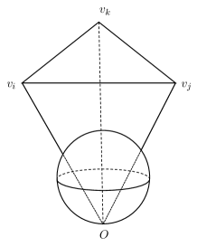
Figure 2. Tetrahedron for PL metric

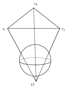
Figure 3. Tetrahedron for PH metric

(2):

For $v_{q}\in\{v_{i},v_{j},v_{k}\}$, if the corresponding $\varepsilon_{q}=1$, then the vertex $v_{q}$ is hyper-ideal and the generalized tetrahedron $T_{Oijk}$ is truncated by a hyperbolic plane $P_{q}$ in $\mathbb{H}^{3}$ dual to $v_{q}$. If $O$ is also hyper-ideal, then it is required that $P_{O}\cap P_{q}=\emptyset$, which is equivalent to the line segment $Ov_{q}$ has nonempty intersection with $\mathbb{H}^{3}$ in the Klein model. If $\varepsilon_{q}=0$, then the vertex $v_{q}$ is ideal and we have a horosphere $H_{q}$ attached to $v_{q}$. For simplicity, we choose the horosphere $H_{q}$ so that it has no intersection with the hyperplane or horospheres attached to the other vertices of $T_{Oijk}$.

(3):

The signed edge length of $Ov_{i},Ov_{j},Ov_{k}$ are $-u_{i},-u_{j},-u_{k}$ respectively.

(4):

For the edge $v_{i}v_{j}$ in the extended hyperbolic space, the weight $\eta_{ij}$ is assigned as follows.

(a):

If $v_{i},v_{j}$ are hyper-ideal and spans a spacelike or lightlike subspace $P_{ij}$, then $\eta_{ij}=\cos\beta_{ij}$, where $\beta_{ij}$ is determined by $-v_{i}\circ v_{j}=||v_{i}||\cdot||v_{j}||\cdot\cos\beta_{ij}$. Here we take $v_{i},v_{j}$ as points in the Minkowski space, $\circ$ is the Lorentzian inner product in the Minkowski space and $||\cdot||$ is the norm of a spacelike vector. In fact, in the case that $v_{i},v_{j}$ spans a spacelike subspace, the hyperbolic planes $P_{i}$ and $P_{j}$, dual to $v_{i}$ and $v_{j}$ respectively, intersect in $\mathbb{H}^{3}$ and $\beta_{ij}$ is the dihedral angle determined by $P_{i}$ and $P_{j}$ in the truncated tetrahedron.

(b):

If $v_{i},v_{j}$ are hyper-ideal and spans a timelike subspace, then $P_{i}$ and $P_{j}$ do not intersect in $\mathbb{H}^{3}$. Denote $\lambda_{ij}$ as the hyperbolic distance of $P_{i}$ and $P_{j}$, then $\eta_{ij}=\cosh\lambda_{ij}=-\frac{v_{i}\circ v_{j}}{||v_{i}||\cdot||v_{j}||}$.

(c):

If $v_{i},v_{j}$ are ideal, we choose the horospheres $H_{i},H_{j}$ at $v_{i},v_{j}$ with $H_{i}\cap H_{j}=\emptyset$ and set $\lambda_{ij}$ to be the distance from $H_{i}\cap\overline{v_{i}v_{j}}$ to $H_{j}\cap\overline{v_{i}v_{j}}$, where $\overline{v_{i}v_{j}}$ is the geodesic from $v_{i}$ to $v_{j}$. Then $\eta_{ij}=\frac{1}{2}e^{\lambda_{ij}}$.

(d):

If $v_{i}$ is ideal and $v_{j}$ is hyper-ideal, we choose the horosphere $H_{i}$ at $v_{i}$ to have no intersection with the hyperbolic plan $P_{j}$ dual to $v_{j}$. Set $\lambda_{ij}$ to be the distance from $H_{i}$ to $P_{j}$. Then $\eta_{ij}=\frac{1}{2}e^{\lambda_{ij}}$.

In this setting, it can be checked that the lengths for the edges in the Euclidean triangle $H_{O}\cap T_{Oijk}$ and in the hyperbolic triangle $P_{O}\cap T_{Oijk}$ are given by (2) and (3) respectively, where $u_{i}=f_{i}$ for the Euclidean background geometry and $u_{i}$ is defined by (63) in terms of $f_{i}$ for the hyperbolic background geometry.

By the hyperbolic cosine laws for generalized hyperbolic triangle $\{v_{i}v_{j}v_{k}\}$, it can be checked that $\eta_{st}+\varepsilon_{s}\varepsilon_{t}>0,\ \varepsilon_{s}\eta_{tq}+\eta_{st}\eta_{sq}>0,\ \{s,t,q\}=\{i,j,k\}.$ This proves Theorem 1.7 (a). We suggest the readers to refer to Appendix A of [18] for a full list of formulas of hyperbolic sine and cosine laws for generalized hyperbolic triangles used here. In the case that $\varepsilon_{i}=\varepsilon_{j}=\varepsilon_{k}=1$, this can be proved in a geometric approach. Note that $\eta_{ij}=-\frac{v_{i}\circ v_{j}}{||v_{i}||\cdot||v_{j}||}$ in this case. Taking $\eta_{ij}+\eta_{ik}\eta_{jk}>0$ for example. Note that

(82) $$\frac{(v_{j}\otimes v_{k})\circ(v_{k}\otimes v_{i})}{||v_{i}||\cdot||v_{j}||\cdot||v_{k}||^{2}}=\left(\frac{v_{j}}{||v_{j}||}\otimes\frac{v_{k}}{||v_{k}||}\right)\circ\left(\frac{v_{k}}{||v_{k}||}\otimes\frac{v_{i}}{||v_{i}}\right)=-(\eta_{ij}+\eta_{ik}\eta_{jk}),$$

where $\otimes$ is the Lorentzian cross product defined by $x\otimes y=J(x\times y)$ with $J=\text{diag}\{-1,1,1\}$ for $x,y\in\mathbb{R}^{3}$. Please refer to [29] (Chapter 3) for more details on Lorentzian cross product. By (82), to prove $\eta_{ij}+\eta_{ik}\eta_{jk}>0$, we just need to prove $(v_{j}\otimes v_{k})\circ(v_{k}\otimes v_{i})<0$. In the following, we use $P_{st}=\text{span}(v_{s},v_{t})$ to denote the two dimensional plane spanned by $v_{s}$ and $v_{t}$ in the Minkowski space. By symmetry, we just need to consider the following six cases.

Figure 4. Generalized triangles

(a):

If $P_{ik}$ and $P_{jk}$ are spacelike, then $v_{j}\otimes v_{k}$, $v_{k}\otimes v_{i}$ are timelike with the same parity. This implies $(v_{j}\otimes v_{k})\circ(v_{k}\otimes v_{i})<0$. Please refer to Figure 4 (a).

(b):

If $P_{ik}$ and $P_{jk}$ are timelike, then $v_{j}\otimes v_{k}$, $v_{k}\otimes v_{i}$ are spacelike and $(v_{j}\otimes v_{k})\circ(v_{k}\otimes v_{i})=-||v_{j}\otimes v_{k}||\cdot||v_{k}\otimes v_{i}||\cdot\cosh d(P_{ik},P_{jk})<0$. Please refer to Figure 4 (b).

(c):

If $P_{ik}$ is spacelike and $P_{jk}$ is timelike, then $v_{j}\otimes v_{k}$ is spacelike and $v_{k}\otimes v_{i}$ is timelike. Then $(v_{j}\otimes v_{k})\circ(v_{k}\otimes v_{i})=-||v_{j}\otimes v_{k}||\cdot|||v_{k}\otimes v_{i}|||\cdot\sinh d<0$, where $|||x|||$ denotes the absolute value of $||x||=(x\circ x)^{1/2}$ for a timelike vector $x$ and $d$ is the distance of $\frac{v_{k}\otimes v_{i}}{|||v_{k}\otimes v_{i}|||}$ to $P_{jk}$. Please refer to Figure 4 (c).

(d):

If $P_{ik}$ is spacelike and $P_{jk}$ is lightlike, then $v_{j}\otimes v_{k}$ is lightlike and $v_{k}\otimes v_{i}$ is timelike with the same parity. This implies $(v_{j}\otimes v_{k})\circ(v_{k}\otimes v_{i})<0$. Please refer to Figure 4 (d).

(e):

If $P_{ik}$ is timelike and $P_{jk}$ is lightlike, then $v_{j}\otimes v_{k}$ is lightlike, $v_{k}\otimes v_{i}$ is spacelike with the same parity as $v_{j}\otimes v_{k}$. Then $(v_{j}\otimes v_{k})\circ(v_{k}\otimes v_{i})<0$. Please refer to Figure 4 (e).

(f):

If $P_{ik}$ is lightlike and $P_{jk}$ is lightlike, then $v_{j}\otimes v_{k}$ is lightlike and $v_{k}\otimes v_{i}$ is lightlike with the same parity as $v_{j}\otimes v_{k}$. Furthermore, $v_{j}\otimes v_{k}$ and $v_{k}\otimes v_{i}$ are linearly independent. Then $(v_{j}\otimes v_{k})\circ(v_{k}\otimes v_{i})<0$. Please refer to Figure 4 (f).

4.2. Convexities of co-volume of generalized hyperbolic tetrahedra

For the generalized hyperbolic tetrahedron $T_{Oijk}$, we have attached it with a generalized hyperbolic polyhedron $\widetilde{P}$ by truncating it by the hyperbolic planes dual to the vertices $O,v_{i},v_{j},v_{k}$. If $\widetilde{P}$ is a generalized hyperbolic polyhedron in $\mathbb{H}^{3}$ with finite volume, we set $\widetilde{P}=P$. Otherwise, the generalized hyperbolic polyhedron $\widetilde{P}$ has hyper-ideal vertices and we need to further truncate $\widetilde{P}$ to get a generalized hyperbolic polyhedron $P$ with finite volume. For example, in the case that $\varepsilon_{i}=\varepsilon_{j}=\varepsilon_{k}=1$, $P_{ij},P_{ik},P_{jk}$ are spacelike, the generalized hyperbolic triangle $\triangle v_{i}v_{j}v_{k}$ has no intersection with $\partial\mathbb{H}^{3}$ and the point $P_{ij}\cap P_{ik}\cap P_{jk}$ is hyper-ideal, we need to use a hyperbolic plane $P_{ijk}$ dual to $P_{ij}\cap P_{ik}\cap P_{jk}$ to truncate $\widetilde{P}$ to get a finite hyperbolic polyhedron $P$.

Denote the volume of the generalized hyperbolic polyhedron $P$ by $V$. By the Schläfli formula [30], we have

$$dV=-\frac{1}{2}(-u_{i}d\theta_{i}-u_{j}d\theta_{j}-u_{k}d\theta_{k}+\lambda_{ij}d\beta_{ij}+\lambda_{ik}d\beta_{ik}+\lambda_{jk}d\beta_{jk}).$$

If $v_{q},v_{s}\in\{v_{i},v_{j},v_{k}\}$ are spacelike and $P_{qs}$ is non-timelike, then $\beta_{qs}$ is fixed, otherwise $\lambda_{qs}$ is fixed. Set

$$\mu_{qs}=\left\{\begin{array}[]{ll}0,&\hbox{ if $\varepsilon_{q}=\varepsilon_{s}=1$ and $P_{qs}$ is non-timelike,}\\ 1,&\hbox{otherwise.}\end{array}\right.$$

Define the co-volume by

(83) $$\widehat{V}=2V-u_{i}\theta_{i}-u_{j}\theta_{j}-u_{k}\theta_{k}+\mu_{ij}\lambda_{ij}\beta_{ij}+\mu_{ik}\lambda_{ik}\beta_{ik}+\mu_{jk}\lambda_{jk}\beta_{jk}.$$

Then we have

(84) $$d\widehat{V}=-\theta_{i}du_{i}-\theta_{j}du_{j}-\theta_{k}du_{k}.$$

By Theorem 2.17 and Theorem 3.13, the equation (84) implies the co-volume function $\widehat{V}$ is convex in $u_{i},u_{j},u_{k}$. As a result, the co-volume function $\widehat{V}$ is convex in the edge lengths $l_{Ov_{i}}=-u_{i},l_{Ov_{j}}=-u_{j},l_{Ov_{k}}=-u_{k}$. This completes the proof of Theorem 1.7 (b).

5. Open problems

5.1. Convergence of Glickenstein’s discrete conformal structures

In [36], Thurston conjectured that the tangential circle packing can be used to approximate the Riemann mapping. Thurston’s conjecture was then proved elegantly by Rodin-Sullivan [31]. Since then, there have been lots of important works on Thurston’s conjecture. See [20, 21, 22] and others. For Luo’s vertex scalings, the corresponding convergence to the Riemann mapping was recently proved by Luo-Sun-Wu [28]. See also [16, 27, 38] for related works. For Bowers-Stephenson’s inversive distance circle packings, the corresponding convergence to Riemann mapping was recently proved by Chen-Luo-Xu-Zhang [4]. Note that Glickenstein’s discrete conformal structures are natural generalizations of Bowers-Stephenson’s inversive circle packings and Luo’s vertex scalings. It is convinced that Thurston’s conjecture is still true for Glickenstein’s discrete conformal structures.

5.2. Discrete uniformization theorems for Glickenstein’s discrete conformal structures

An interesting question about Glickenstein’s discrete conformal structures on polyhedral surfaces is the existence of a discrete conformal factor with the prescribed combinatorial curvature. In the special case that the prescribed combinatorial curvature is constant, this corresponds to the discrete uniformization theorem. For Luo’s vertex scaling, the discrete uniformization theorems were established in [14, 15, 32]. Note that Luo’s vertex scalings correspond to $\varepsilon\equiv 1$ in Glickenstein’s discrete conformal structures. This motivates us to study the discrete uniformization theorem for Glickenstein’s discrete conformal structures.

Suppose $(M,V)$ is a marked surface and $V$ is a nonempty finite subset of $M$. A weight $\varepsilon:V\rightarrow\{0,1\}$ is defined on $V$. The triple $(M,V,\varepsilon)$ is called a weighted marked surface. Motivated by Glickenstein’s works [8, 9, 10, 12], we have the following definition of weighted Delaunay triangulation.

Definition 5.1.

Suppose $(M,V,\varepsilon)$ is a weighted marked surface with a PL metric $d$, and $\mathcal{T}$ is a geometric triangulation of $(M,V,\varepsilon)$ with every triangle $\{ijk\}\in\mathcal{T}$ have a well-defined geometric center $C_{ijk}$. Suppose $\{ij\}$ is an edge shared by two adjacent Euclidean triangles $\{ijk\}$ and $\{ijl\}$. The edge $\{ij\}$ is called weighted Delaunay if $h_{ij,k}+h_{ij,l}\geq 0$, where $h_{ij,k},h_{ij,l}$ are the signed distance of $C_{ijk},C_{ijl}$ to the edge $\{ij\}$ respectively. The triangulation $\mathcal{T}$ is called weighted Delaunay in $d$ if every edge in the triangulation is weighted Delaunay.

One can also define the weighted Delaunay triangulation using the power distance in Remark 2.3. For a PL metric $d$ on $(M,V,\varepsilon)$, its weighted Voronoi decomposition is defined to be the connection of 2-cells $\{R(v)|v\in V\}$, where $R(v)=\{x\in M|\pi_{v}(x)\leq\pi_{v^{\prime}}(x)\ \text{for all }v^{\prime}\in V\}$ is defined by the power distance. The dual cell-decomposition $\mathcal{C}(d)$ of the weighted Voronoi decomposition is called the weighted Delaunay tessellation of $(M,V,\varepsilon,d)$. A weighted Delaunay triangulation $\mathcal{T}$ of $(M,V,\varepsilon,d)$ is a geometric triangulation of the weighted Delaunay tessellation $\mathcal{C}(d)$ by further triangulating all non-triangular 2-dimensional cells without introducing extra vertices. As the power distance is a generalization of Euclidean distance, the weighted Delaunay triangulation is a generalization of the Delaunay triangulation.

Following Gu-Luo-Sun-Wu [15], we introduce the following new definition of discrete conformality, which allows the triangulation of the weighted marked surface $(M,V,\varepsilon)$ to be changed.

Definition 5.2.

Two piecewise linear metrics $d,d^{\prime}$ on $(M,V,\varepsilon)$ are discrete conformal if there exist sequences of PL metrics $d_{1}=d$, $\cdots$, $d_{m}=d^{\prime}$ on $(M,V,\varepsilon)$ and triangulations $\mathcal{T}_{1},\cdots,\mathcal{T}_{m}$ of $(M,V,\varepsilon)$ satisfying

(a):

(Weighted Delaunay condition) each $\mathcal{T}_{i}$ is weighted Delaunay in $d_{i}$,

(b):

(Discrete conformal condition) if $\mathcal{T}_{i}=\mathcal{T}_{i+1}$, there exists two functions $u_{i},u_{i+1}:V\rightarrow\mathbb{R}$ such that if $e$ is an edge in $\mathcal{T}_{i}$ with end points $v$ and $v^{\prime}$, then the lengths $l_{d_{i+1}}(e)$ and $l_{d_{i}}(e)$ of $e$ in $d_{i}$ and $d_{i+1}$ are defined by (2) using $u_{i}$ and $u_{i+1}$ respectively with the same weight $\eta:E\rightarrow\mathbb{R}$.

(c):

if $\mathcal{T}_{i}\neq\mathcal{T}_{i+1}$, then $(S,d_{i})$ is isometric to $(S,d_{i+1})$ by an isometry homotopic to identity in $(S,V)$.

The space of PL metrics on $(M,V,\varepsilon)$ discrete conformal to $d$ is called the conformal class of $d$ and denoted by $\mathcal{D}(d)$.

Motivated by Gu-Luo-Sun-Wu’s discrete uniformization theorem for vertex scalings of PL metrics in [15], we have the following conjecture on the discrete uniformization for Glickenstein’s Euclidean discrete conformal structures on weighted marked surfaces.

Conjecture 5.3.

Suppose $(M,V,\varepsilon)$ is a closed connected weighted marked surface with $\varepsilon:V\rightarrow\{0,1\}$, $\chi(M)=0$ and $d$ is a PL metric on $(M,V,\varepsilon)$. There exists a PL metric $d^{\prime}\in\mathcal{D}(d)$, unique up to scaling and isometry homotopic to the identity on $(M,V,\varepsilon)$, such that $d^{\prime}$ is discrete conformal to $d$ and the combinatorial curvature of $d^{\prime}$ is $0$.

For the hyperbolic background geometry, one can define the corresponding weighted Delaunay triangulation and the corresponding discrete conformality similarly. We have the following conjecture on the discrete uniformization for Glickenstein’s hyperbolic discrete conformal structures on weighted marked surfaces.

Conjecture 5.4.

Suppose $(M,V,\varepsilon)$ is a closed connected weighted marked surface with $\varepsilon:V\rightarrow\{0,1\}$, $\chi(M)<0$ and $d$ is a PH metric on $(M,V,\varepsilon)$. There exists a unique PH metric $d^{\prime}\in\mathcal{D}(d)$ on $(M,V,\varepsilon)$ so that $d^{\prime}$ is discrete conformal to $d$ and the combinatorial curvature of $d^{\prime}$ is 0.

One can also study the prescribing combinatorial curvature problem for Glickenstein’s discrete conformal structures on polyhedral surfaces. Results similar to the results in [14, 15, 35] are convinced to be true for Glickenstein’s discrete conformal structures on polyhedral surfaces.

References

- [1] A. Bobenko, U. Pinkall, B. Springborn, Discrete conformal maps and ideal hyperbolic polyhedra. Geom. Topol. 19 (2015), no. 4, 2155-2215.
- [2] A.I. Bobenko, B.A. Springborn, Variational principles for circle patterns and Koebe’s theorem, Trans. Amer. Math. Soc. 356 (2) (2004) 659-689.
- [3] P. L. Bowers, K. Stephenson, Uniformizing dessins and Belyĭ maps via circle packing. Mem. Amer. Math. Soc. 170 (2004), no. 805.
- [4] Y. Chen, Y. Luo, X. Xu, S. Zhang, Bowers-Stephenson’s conjecture on the convergence of inversive distance circle packings to the Riemann mapping, arXiv:2211.07464 [math.GT].
- [5] B. Chow, F. Luo, Combinatorial Ricci flows on surfaces, J. Differential Geometry, 63 (2003), 97-129.
- [6] J. Dai, X. Gu, F. Luo, Variational principles for discrete surfaces, Advanced Lectures in Mathematics (ALM), vol. 4, International Press/Higher Education Press, Somerville, MA/Beijing, 2008, iv+146 pp.
- [7] Y. C. de Verdière, Un principe variationnel pour les empilements de cercles, Invent. Math. 104(3) (1991) 655-669
- [8] D. Glickenstein, A combinatorial Yamabe flow in three dimensions, Topology 44 (2005), No. 4, 791-808.
- [9] D. Glickenstein, A monotonicity property for weighted Delaunay triangulations. Discrete Comput. Geom. 38 (2007), no. 4, 651-664.
- [10] D. Glickenstein, Discrete conformal variations and scalar curvature on piecewise flat two and three dimensional manifolds, J. Differential Geom. 87 (2011), no. 2, 201-237.
- [11] D. Glickenstein, Euclidean formulation of discrete uniformization of the disk, Geom. Imaging Comput. 3 (2016), no. 3-4, 57-80.
- [12] D. Glickenstein, Geometric triangulations and discrete Laplacians on manifolds, arXiv:math/0508188 [math.MG].
- [13] D. Glickenstein, J. Thomas, Duality structures and discrete conformal variations of piecewise constant curvature surfaces. Adv. Math. 320 (2017), 250-278.
- [14] X. D. Gu, R. Guo, F. Luo, J. Sun, T. Wu, A discrete uniformization theorem for polyhedral surfaces II, J. Differential Geom. 109 (2018), no. 3, 431-466.
- [15] X. D. Gu, F. Luo, J. Sun, T. Wu, A discrete uniformization theorem for polyhedral surfaces, J. Differential Geom. 109 (2018), no. 2, 223-256.
- [16] X. D. Gu, F. Luo, T.Wu, Convergence of discrete conformal geometry and computation of uniformization maps. Asian J. Math. 23 (2019), no. 1, 21-34.
- [17] R. Guo, Local rigidity of inversive distance circle packing, Trans. Amer. Math. Soc. 363 (2011) 4757-4776.
- [18] R. Guo, F. Luo, Rigidity of polyhedral surfaces. II, Geom. Topol. 13 (2009), no. 3, 1265-1312.
- [19] X. He, X. Xu, Thurston’s sphere packings on 3-dimensional manifolds, I, Calc. Var. Partial Differential Equations. 62 (2023), no. 5, Paper No. 152, 23 pp.
- [20] Z.-X. He, Rigidity of infinite disk patterns. Ann. of Math. (2) 149 (1999), no. 1, 1-33.
- [21] Z.-X. He, O. Schramm, On the convergence of circle packings to the Riemann map. Invent. Math., 125 (1996), 285-305.
- [22] Z.-X. He, O. Schramm, The -convergence of hexagonal disk packings to the Riemann map, Acta Math. 180 (1998) 219-245.
- [23] G. Leibon, Characterizing the Delaunay decompositions of compact hyperbolic surface. Geom. Topol. 6 (2002), 361-391.
- [24] F. Luo, Combinatorial Yamabe flow on surfaces, Commun. Contemp. Math. 6 (2004), no. 5, 765-780.
- [25] F. Luo, Rigidity of polyhedral surfaces, III, Geom. Topol. 15 (2011), 2299-2319.
- [26] F. Luo, Rigidity of polyhedral surfaces, I. J. Differential Geom. 96 (2014), no. 2, 241-302.
- [27] F. Luo, The Riemann mapping theorem and its discrete counterparts. From Riemann to differential geometry and relativity, 367-388, Springer, Cham, 2017.
- [28] F. Luo, J. Sun, T. Wu, Discrete conformal geometry of polyhedral surfaces and its convergence, Geom. Topol. 26 (2022), no. 3, 937-987.
- [29] John G. Ratcliffe, Foundations of hyperbolic manifolds. Second edition. Graduate Texts in Mathematics, 149. Springer, New York, 2006. xii+779 pp. ISBN: 978-0387-33197-3; 0-387-33197-2.
- [30] I. Rivin, Euclidean structures of simplicial surfaces and hyperbolic volume. Ann. of Math. 139 (1994), 553-580.
- [31] B. Rodin, D. Sullivan, The convergence of circle packings to the Riemann mapping, J. Differential Geom. 26 (1987) 349-360.
- [32] B. Springborn, Ideal hyperbolic polyhedra and discrete uniformization. Discrete Comput. Geom. 64 (2020), no. 1, 63-108.
- [33] K. Stephenson, Introduction to circle packing. The theory of discrete analytic functions. Cambridge University Press, Cambridge, 2005.
- [34] J. Thomas, Conformal variations of piecewise constant two and three dimensional manifolds, Thesis (Ph.D.), The University of Arizona, 2015, 120 pp.
- [35] W. Thurston, Geometry and topology of -manifolds, Princeton lecture notes 1976, http://www.msri.org/publications/books/gt3m.
- [36] W. Thurston, The finite Riemann mapping theorem. An International Symposium at Purdue University on the Occasion of the Proof of the Bieberbach Conjecture, 1985.
- [37] E.B. Vinberg, Geometry. II, Encyclopaedia of Mathematical Sciences, 29, Springer-Verlag, New York, 1988.
- [38] T. Wu, X. Zhu, The convergence of discrete uniformizations for closed surfaces, arXiv:2008.06744v2 [math.GT]. To appear in J. Differential Geom.
- [39] X. Xu, Rigidity of inversive distance circle packings revisited, Adv. Math. 332 (2018), 476-509.
- [40] X. Xu, A new proof of Bowers-Stephenson conjecture, Math. Res. Lett. 28 (2021), no. 4, 1283-1306.
- [41] X. Xu, Deformation of discrete conformal structures on surfaces, preprint, 20 pages.
- [42] X. Xu, C. Zheng, A new proof for global rigidity of vertex scaling on polyhedral surfaces, Asian J. Math. 25 (2021), no. 6, 883-896.
- [43] X. Xu, C. Zheng, On the classification of discrete conformal structures on surfaces, arXiv:2307.13223 [math.DG].
- [44] M. Zhang, R. Guo, W. Zeng, F. Luo, S.T. Yau, X. Gu, The unified discrete surface Ricci flow, Graphical Models 76 (2014), 321-339.