Baryon production in the quantized fragmentation of helical QCD string

Abstract

Baryon production is studied within the framework of quantized fragmentation of QCD string. Baryons appear in the model in a fairly intuitive way, with help of causally connected string breakups. A simple helical approximation of QCD flux tube with parameters constrained by mass spectrum of light mesons is sufficient to reproduce masses of light baryons.

1 Introduction

The idea to model the confinement with help of helical string has been proposed by Lund theorists in [1]. Causal approach to the ordering of string breakup vertices reveals that mass spectrum of light hadrons corresponds to breaking of string in pieces with quantized (helix) phase difference [2].

For better understanding of the difference between the Lund string model [3], widely used by the particle physics community, and its quantized helical spin-off, a brief overview of definitions and assumptions is provided.

In close analogy with Lund string fragmentation, the momentum acquired by massless quarks moving along the helical string amounts to the integral of the string tension tangential to the string curvature. The non-trivial part of the integral between vertices A,B is the transverse momentum

$$\vec{p}_{T} = \kappa R\int_{A}^{B}\exp{i(\Phi\pm\pi/2)}d\Phi$$ (1)

$$= 2\kappa R\sin{\frac{\Phi_{B}-\Phi_{A}}{2}}\exp{i(\frac{\Phi_{A}+\Phi_{B}\pm\pi}{2})},$$

where $\kappa\sim$1 GeV/fm stands for string tension, $R$ is the radius of helix and $\Phi$ designs the helix phase. The $\pm$ sign distinguishes movement of quarks and antiquarks. The transverse and longitudinal momentum components decouple, and quark acquires an effective mass entirely derived from transversal properties of the string

$$m_{AB}=\kappa R\sqrt{(\Phi_{B}-\Phi_{A})^{2}-(2\sin{\frac{\Phi_{B}-\Phi_{A}}{2}})^{2}}.$$ (2)

The 3-dimensional string plays essential role in the model by allowing to introduce causality in the description of the fragmentation process - the use of 1-dimensional string to model the confinement in the standard Lund fragmentation model implies that breakup-vertices forming a hadron are - by construction! - causally disconnected.

The causal description of hadron formation turns out to be an excellent guiding principle in the model-building. If we let the information about string breakup run along the string together with newly created quark, the requirement of causal connection between breakup vertices implies the subsequent breakup is triggered by the propagating quark. Such a production mechanism seems suitable for narrow resonant states with mass given by Eq.2. The difference between spontaneous (uncorrelated) and induced (correlated) string breakup is shown on diagrams in Fig. 1.

Figure 1: Schema of hadron creation via uncorrelated (left) and correlated (right) string breakups. Green band indicates the color flow ordering of the gluon ladder. Excited gluon – which splits promptly into a $Q\bar{Q}$ pair – is marked in red.

It is remarkable that it is the causal reformulation of the string fragmentation rules that actually reveals the quantized nature of the process. Comparing mass spectra of light mesons with string parametrization, it becomes clear that fragmentation proceeds in distant steps in helix phase difference, $\Phi_{B}-\Phi_{A}=n\Delta\Phi,n=1,2,3,..$. The (transverse sector of) quantized string can therefore be described with help of just two parameters, energy scale $\kappa R$ and the phase quantum $\Delta\Phi$.

The model is particularly interesting from the phenomenological point of view since it is empirically overconstrained: the number of sensitive observables vastly outnumbers the number of adjustable parameters. On one side, we have hadron mass spectra: pseudoscalar mesons ($\pi,\eta,\eta^{\prime}$) can be associated with quantum states ($n$=1,3,5), vector meson $\omega$ fills the slot $n$=4. On the other side, the underlying helical field defines intrinsic transverse momenta of hadrons and, for specific configurations - homogeneous or slowly evolving helical field - dominates the correlations between hadrons as function of their relative position along the string.

Before moving on to the discussion of phenomena which can be explained by the model, a disclaimer should be issued about what the model does not describe - not because it is fundamentally defficient, but because a priority is given to a broad exploration of predictions stemming from the simple core concept of quantized fragmentation. Detailed description of $qg\rightarrow qq\bar{q}$ interaction is not included which means the model is blind to the mass difference between charged and neutral pions - this is essentially setting the limit of the precision of predictions, at the level of $\sim$3%. Such a precision is comparable with the precision of experimental measurements of correlations between adjacent hadrons, and therefore sufficient for the purpose of the current study.

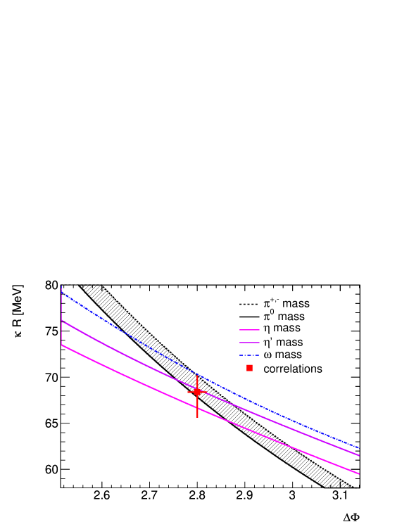
Figure 2: An overview of constraints imposed on model parameters by hadron mass spectrum [4] and by the measurement of correlations between adjacent hadrons [5]. The dashed region indicates the internal precision of model predictions.

Figure 2 shows the overview of constraints imposed on helix parameters by hadron masses [4] and by the measurement of correlations between adjacent hadrons [5] (see Appendix A for the extraction of parameters from the measurement). Please note the measured correlations cover, among other, the entire anomalous production of close like-sign pion pairs, traditionally attributed to the Bose-Einstein interference.

Figure 3: Schema of correlated(induced) string breakup across string loops. Green band indicates the color flow ordering of the gluon ladder. Excited gluon – which splits promptly into a $Q\bar{Q}$ pair – is marked in red.

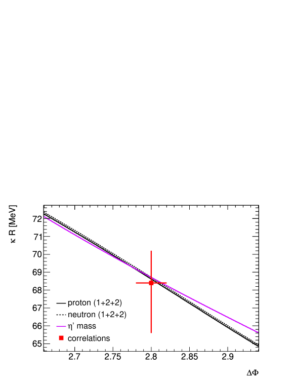
Figure 4: Top: Example of string breakup leading to creation of a nucleon (2+2+1) in forward direction. Bottom: Constraints imposed on model parameters by (2+2+1) nucleon hypothesis, compared with those stemming from $\eta^{\prime}$ mass and from the measured correlations between adjacent hadrons [5].

2 Baryon production

In the introduction, the causal connection between string breakup vertices was limited to the information transfer along the string. It is however possible that such an transfer occurs across the string loops, in particular for string configuration with dense packing (small pitch). This type of induced string breakup is shown in Fig. 3. The net result of such an interaction is a coherent production of three partons ($qQ\bar{Q}$ or $\bar{q}Q\bar{Q}$, where $q$ and $\bar{q}$ indicate the propagating parton which triggers the interaction). For the production of a pair of baryons, it is therefore sufficient to consider an initial string breakup ($g\rightarrow q\bar{q}$) followed by two induced gluon splittings across string loops. The integration over longitudinal component of the string field contributes to the separation of quark and antiquark momenta ( running forward and backward along the string), and this may facilitate creation of bound states composed of colour neutral combinations of quarks or antiquarks only, the baryons.

The lightest baryons (nucleons) have masses which slightly exceed mass of two string loops ( $4\pi\kappa R\sim$ 0.9 GeV, using the measurement [5] ). The proximity with mass of $\eta^{\prime}$ suggests that these particles are formed by 5 quanta of quantized helical string. Several possible production mechanisms are investigated below. They differ by the redistribution of initial momentum between partons. Please note that impact of quark masses on the mass of hadrons diminishes as hadrons become heavier : the mass difference between neutron and proton is only 1.3‰. If the model is capturing the dynamics of hadron formation correctly, we may also expect the precision of model predictions to improve for heavier hadrons.

2.1 Case (1+2+2)

The first example of possible string breaking scheme for a nucleon formation is $q(\bar{q})q(\bar{q})q(\bar{q})$=1(1)2(2)2(2) - this compact notation is used to describe the forward/$qqq$ and (backward/$\bar{q}\bar{q}\bar{q}$) baryon simultaneously. The break-up pattern and the mass constraints on model parameters corresponding to nucleon moving in forward direction ($qqq$, by convention) are shown in Fig. 4(string breakup is modelled via gluon splitting $g\rightarrow q\bar{q}$). The nucleon mass dependence on model parameters nearly coincides with the curve calculated for $\eta^{\prime}$ meson, which is very encouraging : the model is working equally well for baryons and mesons. It seems, nevertheless, that this solution is not quite optimal, because the forward and backward configurations are not symmetric and their masses differ by $\sim$2%.

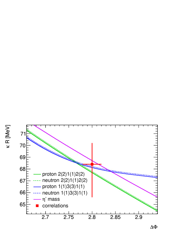
Figure 5: Top: (2+1+2) and (1+3+1) nucleon formation scenarios, symmetrized with respect to ($qqq$/$\bar{q}\bar{q}\bar{q}$) production. Bottom: Constraints imposed on model parameters by these nucleon production scenarios, compared with those stemming from $\eta^{\prime}$ mass and from the measured correlations between adjacent hadrons [5].

2.2 Symmetrization (2+1+2) & (1+3+1)

The string breaking pattern can be symmetrized with respect to $qqq$ / $\bar{q}\bar{q}\bar{q}$ production as shown in Fig. 5 for (2+1+2) and (1+3+1) nucleon production scenarios. In both cases, we obtain a baryon/antibaryon pair with parametrization matching the meson production and correlation measurements, within $\sim$1% precision tolerance.

2.3 $\Lambda$-like configurations

With a simple modification of the nucleon breaking pattern, a $\Lambda$-like baryon can be produced. An example is shown in Fig. 6 using 2(1)3(3)1(2) split pattern which produces a pair of baryons with $\Lambda$ mass. Even more intriguingly, $\Lambda$ production can be mimicked by a simple chain production of proton and pion, where the unbound state also ends up with mass of $\Lambda$. Without a detailed production mechanism for $s\bar{s}$ introduced in the model (subject of a separate publication), the discussion of $\Lambda$ production is premature, however it seems that (a) it is very likely that strangeness can be introduced in the model without a major perturbation of the string parametrization, (b) $\Lambda$ production can be to some extent mimicked by baryon production involving light(massless) quark pairs only, or even by unbound production of ($p/n+\pi$) pair with rank difference 2 (the rank of direct hadrons refers to their ordering along the fragmenting string, according to the colour flow).

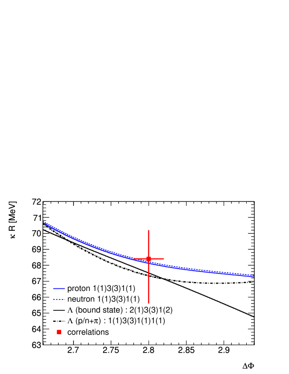
Figure 6: Top: $\Lambda\bar{\Lambda}$-like string splitting scenarios, bound (1+3+2) and unbound (1+3+1+1)=(p+$\pi$). Bottom: Constraints imposed on model parameters by requiring that these configurations acquire mass of $\Lambda$ baryon, compared with those stemming from nucleon mass and from the measured correlations between adjacent hadrons [5].

3 Discussion: mass spectra of light hadrons

With the extension of the model to the baryon production - which turns out to be simply a consistency check, since nucleons appear just where one would expect them, when interactions across string loops are admitted - the matching of light hadrons to the quantized fragmentation scheme is nearly complete. In Fig. 7, mass spectrum is plotted as function of the number of string quanta involved in hadron formation. Colors are used to distinguish set of hadrons with similar production mechanism: in red, pseudoscalar mesons ($\pi,\eta,\eta^{\prime}$) and vector meson $\omega$ for coherent string “light front” breaking. The red dashed line indicates the (non-quantized) mass dependence on the helix phase difference. Baryons produced via coherent string breaking across string loops are shown in blue. Wide resonant states ($f_{0},\rho$), in green, are presumably produced via incoherent string breaking: in such a scenario, mass of hadron is not uniquely defined by the tranverse shape of the string, it also depends on longitudinal properties of the string. Indeed, the $\rho$ mass measurements differ in $\tau$ decays and hadroproduction [4].

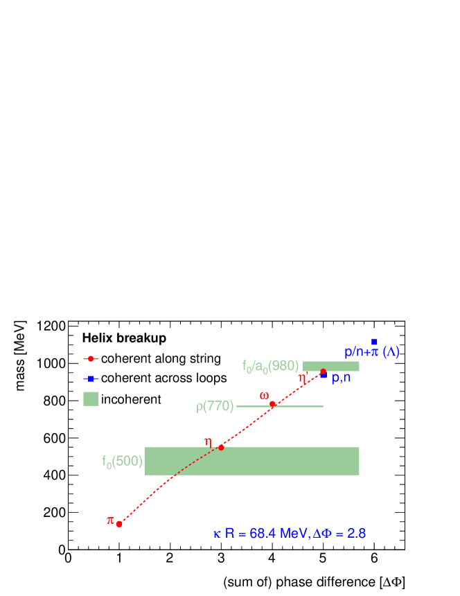
Figure 7: Light hadrons classified according to presumed production mechanism in the model of helical QCD string, plotted as function of the (quantized) helix phase difference between breakup vertices. For baryons, the phase difference is summed over three string pieces. Coherent string breakup defines the hadron mass (red dashed line) as function of transverse string parameters, wide resonant states (f₀,$\rho$) have mass influenced by the longitudinal string properties. Calculations done with string parameters ($\kappa R,\Delta\Phi$) measured via hadron correlations [5].

Having the light hadron mass spectrum and part of hadron correlations described by just two parameters with a precision of few percent is certainly an attractive feature of the model, allowing to reduce the number of parameters needed for description of data. It is also an opportunity to reconsider the approach to soft QCD, mostly because it seems difficult to reconcile the quantized fragmentation with the conventional picture of colour field consisting of ( nonperturbative ) sea of soft gluons. What would prevent any of these gluons to produce a random breakup, which would then prevail over coherent string breaking ? In fact, the arguments tend to support just the opposite - a minimalist description of string with density of gluons as low as two per $\Delta\Phi$. For the argumentation we do not need to reach further than the original helix paper [1]. One of the main arguments of the authors was the effective absence of collinear gluon emission at the end of the parton cascade. They evaluated the minimal distance between colour connected gluons to be 11/6 (1.83), which is just 8% smaller than the measured value $2\sin{(\Delta\Phi/2)}=$1.97. The space between gluons, according to the discussion in [1], is effectively occupied by the accompanying Coulomb field. For a creation of lightest hadron ($qg\bar{q}$) , at least one additional accompanying gluon is needed in each $\Delta\Phi$ interval. An effective density of 1 gluon per $\Delta\Phi/2\sim$1.4 is also roughly consistent with the non-collinear emission of gluons by quarks, where the effective depleted zone around quark is 3/2. In the original paper, authors did not deploy the causal constraint, and concentrated on the parametrization of the longitudinal separation of partons in $\Delta y$ instead. The quantized fragmentation is extending the argument to the limit of $\Delta y\rightarrow$0 by fully exploiting the azimuthal degree of freedom.

4 Further experimental evidence

In the model of quantized fragmentation of a helical QCD string, transverse momenta of hadrons (w.r.t. string axis) are constrained and predicted with a similar precision as their masses. Since the measurement of these intrinsic transverse momenta is conditioned by the precision with which the axis of the generating QCD string can be determined, the measurement is not expected to improve the precision of constraints derived from hadron mass spectrum and from measurement of correlations between hadrons as described above. Nevertheless, study of pencil-like events in LEP data or soft minimum bias events at LHC may provide an interesting cross-check of model predictions, which are gathered in Table 1. All calculations are done assuming ideal helix shape without additional complex structures (knots).

Table 1: Model prediction for intrinsic transverse momentum of direct hadrons, for measured (Appendix A) string parameters.

hadron	production mode	quantized content [$\Delta\Phi$]	$p_{T}$ [MeV]
$\pi$	induced, light-front	1	135 (+4,-6)
$\eta$	induced, light-front	3	119 (+3,-5)
$\omega$	induced, light-front	4	86 (+2,-4)
$\eta^{\prime}$	induced, light-front	5	90 (+3,-4)
p,n	induced, across loop	1+2+2	206 (+6,-9)
p,n	induced, across loop	2+1+2	135 (+4,-6)
p,n	induced, across loop	1+3+1	172 (+5,-7)
$\Lambda$	induced, across loop	1+3+2	208 (+6,-9)

5 Conclusions

The production of light baryons using the hypothesis of correlated helical string breaking with information passing across helix loops has been investigated. Nucleons (p,n) can be described by a combination of three coherently produced fragments of helical string, which jointly carry 5 string quanta. Model is using ideal helix shape and massless parton approximation. Despite the model simplicity, masses of light hadrons below 1 GeV agree with model predictions within 3% and the agreement is even better ($\sim$1%) for baryons. No addditional parameters nor readjustment of string parameterization are needed to accommodate the baryon production.

It is argued that the ideal helix approximation can be a proxy for a low density gluon chain, with approximately two gluons per $\Delta\Phi$. Such a simplified description of the confining field should be of interest for hadronization models and for calculations of parton density functions (PDF) within nucleon.

Appendix A Model parameters measured with help of hadron correlations

Correlations between pairs of hadrons(pions) with rank difference 1 and 2 have been measured [5] in hadron chains selected via mass minimization and matched with the anomalous production of like-sign (LS) pairs. Charge ordering of hadrons implies opposite-sign (OS) pairs correspond to rank difference 1, and LS pairs to rank difference 2. The measured value of momentum difference is (266${}^{+8}_{-11}$) MeV for OS pairs, and (89.7${}^{+2.5}_{-3.5}$) MeV for LS pairs.

In the limit of homogeneous string field (constant helix pitch), the momentum difference between pion pairs with rank difference $n$ can be written as [2]

$$Q(n)=2\ p_{\mathrm{T}}(n=1)\ \sin{(n\Delta\Phi/2)}\\$$ (3)

The ratio

$$\frac{Q(n=1)}{Q(n=2)}=\frac{\sin{(\Delta\Phi/2)}}{\sin{(\Delta\Phi)}}=2.96\pm 0.15$$ (4)

implies $\Delta\Phi=2.80\pm 0.02$. Taking into account Eq.1, the energy scale estimate is $\kappa R=68.4^{+1.8}_{-2.8}$ GeV .

References

- [1] B. Andersson, G. Gustafson, J. Häkkinen, M. Ringner and P. Sutton, Is there screwiness at the end of the QCD cascades?, JHEP9809(1998) 014.
- [2] Š. Todorova-Nová, Quantization of the QCD string with a helical structure, Phys.Rev.D89(2014) 015002.
- [3] B. Andersson et al., Parton Fragmentation and String Dynamics, Phys.Rept.97(1983) 31.
- [4] Particle Data Group, Review of Particle Physics, Phys.Rev.D98(2018) 030001.
- [5] ATLAS Collaboration, Study of ordered hadron chains with the ATLAS detector, Phys.Rev.D96(2017) 092008.