Red supergiants in M31 and M33 II. The Mass Loss Rate

Abstract

Mass loss is an important activity for red supergiants (RSGs) which can influence their evolution and final fate. Previous estimations of mass loss rates (MLRs) of RSGs exhibit significant dispersion due to the difference in method and the incompleteness of sample. With the improved quality and depth of the surveys including the UKIRT/WFCAM observation in near infrared, LGGS and PS1 in optical, a rather complete sample of RSGs is identified in M31 and M33 according to their brightness and colors. For about 2000 objects in either galaxy from this ever largest sample, the MLR is derived by fitting the observational optical-to-mid infrared spectral energy distribution (SED) with the DUSTY code of a 1-D dust radiative transfer model. The average MLR of RSGs is found to be around $2.0\times 10^{-5}{\text{M}_{\odot}}/\text{yr}$ with a gas-to-dust ratio of 100, which yields a total contribution to the interstellar dust by RSGs of about $1.1\times 10^{-3}{\text{M}_{\odot}}/\text{yr}$ in M31 and $6.0\times 10^{-4}{\text{M}_{\odot}}/\text{yr}$ in M33, a non-negligible source in comparison with evolved low-mass stars. The MLRs are divided into three types by the dust properties, i.e. amorphous silicate, amorphous carbon and optically thin, and the relations of MLR with stellar parameters, infrared flux and colors are discussed and compared with previous works for the silicate and carbon dust group respectively.

1 Introduction

Mass loss is a common phenomena of RSGs, evidenced by the observed infrared excess firstly in NML Cyg and VY CMa (Johnson, 1968; Hyland et al., 1969) and lately in numerous RSGs. The destiny of a RSG depends on mass loss rate in addition to initial mass and chemical composition. Some RSGs may stay in the RSG stage and eventually explode as hydrogen-rich Type II-P supernovae (SNe), while the others may evolve backwards to the blue end of the H-R diagram and spend some short time as yellow supergiant stars (YSGs), blue supergiant stars (BSGs) or Wolf-Rayet stars (WRs) before exploding as SNe (Smartt, 2009; Humphreys, 2010; Ekström et al., 2013; Meynet et al., 2015; Beasor & Davies, 2018). In either case, the strong mass loss during the RSG phase would greatly influence its ultimate fate. Moreover, the mass loss of RSGs significantly contribute to the interstellar dust content, in particular in young galaxies at high redshift where the potential dust producer — asymptotic giant branch stars (AGBs) are not yet evolved (Massey et al., 2005; Levesque, 2010).

There have been various types of methods to estimate the mass loss rate (MLR, expressed as mass loss per year ${\rm M_{\odot}/yr}$) of RSGs from their infrared emission that increases with the amount of dust. One type fits the spectral energy distribution (SED) by a dust radiative transfer model (see e.g. Gordon et al. 2018). Alternatively, spectrum analysis may be used to derive mass loss rate with the shell expansion velocities determined from the spectral line, e.g. OH double-peak maser (Goldman et al., 2017). The classical Reimers law (Reimers, 1975; Kudritzki & Reimers, 1978) was derived from high resolution spectroscopy from which stellar wind outflow velocities and circumstellar line optical depths were determined. There are some empirical relations between the mass loss rate and stellar parameters such as luminosity or effective temperature, which is usually based on the results from the SED fitting.

RSGs in the Milky Way are the nearest though suffering heavy interstellar extinction in the Galactic plane. Still, some of them are close enough to be observed in multiple bands or even spatially resolved. The calculation leads to high MLR for some famous RSGs. Gordon et al. (2018) estimated the MLR of VX Sgr, NML Cyg and S Per from infrared imaging to be $2\sim 3\times 10^{-5}{\rm M_{\odot}/yr}$ on average. Beasor & Davies (2018) studied the RSGs in the clusters NGC 7419 and $\chi$ Per yielding the MLR from $10^{-7}{\rm M_{\odot}/yr}$ to $10^{-5}{\rm M_{\odot}/yr}$ and found a steep increase of MLR with stellar luminosity. For RSGs in the Large Magellanic Cloud (LMC), van Loon et al. (2005) derived the MLR to range mostly in $10^{-4}\text{to}10^{-5}{\rm M_{\odot}/yr}$ for a sample of about 15 dust-enshrouded RSGs in the LMC by using the DUSTY code, a dust radiative transfer model (Ivezic & Elitzur, 1997). While for a large sample ($\sim$ 30,000) of AGBs and RSGs in the LMC, Riebel et al. (2012) used the GRAMS grids and obtained a dust mass loss rate mostly between $10^{-7}\text{to}10^{-11}{\rm M_{\odot}/yr}$, a much lower MLR than by van Loon et al. (2005). Gordon et al. (2016) studied the RSGs in M31 and M33 and found the massive RSGs have an average mass loss rate of $10^{-4}{\rm M_{\odot}/yr}$ to $10^{-5}{\rm M_{\odot}/yr}$. Groenewegen & Sloan (2018) estimated a mass loss rate between $10^{-4}\text{to}10^{-10}{\rm M_{\odot}/yr}$ of RSGs and AGBs in LMC, SMC and dwarf spheroidal galaxies in the Local Group.

The large range of MLR in previous studies (from about $10^{-11}{\rm M_{\odot}/yr}$ to $10^{-4}{\rm M_{\odot}/yr}$) originated from the distinction in the RSGs sample, the dust properties, the models and so on. In common, previous studies selected only a small portion of RSGs, mostly bright in optical and/or infrared, which would incline to the high MLR cases and cannot reflect the overall situation of MLR of RSGs unbiasedly. The difference in method also brings about the difficulty in comparing the results mutually. Ren et al. (2021, hereafter Paper I) constructed a sample of RSGs in M31 and M33 based mainly on the near-infrared color-color diagram and the Gaia astrometric information, which is claimed to be complete. This provides us the opportunity of investigating the MLR of all the RSGs in an individual galaxy. Besides, both M31 and M33 are spiral galaxies with similar metallicity to our Milky Way galaxy whose entire scenario cannot be viewed from internal, this would shed light on the MLR, the properties of RSGs dust and their contribution to ISM in our Galaxy. This work intends to calculate the MLR for a couple of thousands of RSGs in M31 and M33 in this newly selected sample the majority of which is identified as a RSG for the first time, and to discuss the circumstellar dust properties and the contribution to interstellar dust by RSGs.

The paper is organized as follows. Section 2 describes the sample, and Section 3 presents the dust model we use. The last section is about the result and some discussion on MLRs of RSGs.

2 Sample

2.1 Preliminary sample

The initial sample of RSGs in M31 and M33 is taken from Paper I. Massey et al. (2006, 2007) selected 437 and 749 RSG candidates in M33 and M31 respectively by optical spectrum and colors. In comparison with the number ($\sim$ 1400) of RSGs in SMC identified by Yang et al. (2018, 2019), the optically selected sample in M31 and M33 is far from complete. Paper I uses the deep UKIRT/WFCAM photometry in the $JHK$ bands and an innovative method to exclude the foreground stars, i.e. to remove the foreground dwarf stars from their obvious branch in the $J-H/H-K$ diagram due to their high surface gravity effect on the $H$ band. Afterwards, RSGs are recognized by their large brightness and low effective temperature, in practice from their location in the $J-K/K$ diagram that coincides well with the theoretical evolutionary track of a massive star. Consequently, Paper I identified 5498 and 3055 RSGs in M31 (along with M32 and M110) and M33 respectively, several times larger than the previous samples. After dropping off the sources outside the areas of M31 and M110, there are 5253 and 3001 RSGs left which forms the initial sample of this work. The details of the selection and discussion on the completeness of the sample is referred to Paper I.

2.2 Final sample: combination of catalogs in various wavebands

The initial sample is further reduced to be appropriate for estimating MLR. In complying with the traditional method, we choose to fit the SED by the dust radiative transfer model. In order to characterize the SED of a RSG, it is better to have the photometric results covering wider wavebands (in particular in the infrared) with higher accuracy. In principle, the optical bands can constrain the properties of the central star while the infrared bands demonstrate the radiation of the dust. The optical photometric data are taken from the Pan-STARRS1 large-scale survey in the $g$, $r$, $i$, $z$ and $y$ bands (Chambers et al., 2016) and the dedicated LGGS survey in the $U$, $B$, $V$, $R$, $I$ bands (Massey et al., 2006, 2007). In addition to the UKIRT/WFCAM photometry in the $J$, $H$ and $K$ bands available for all the objects, the photometry at relatively longer wavelengths is taken from the Spitzer/IRAC (IRAC1, IRAC2, IRAC3 and IRAC4) (Werner et al., 2004), Spitzer/MIPS24 (Rieke et al., 2004) and WISE (W1, W2, W3)(Wright et al., 2010) observations. The WISE/W4 photometry is not used because its flux is usually much higher than that of the Spitzer/MIPS24, which may be caused by the low resolution in this band. These data consist an SED from optical-violet (366nm) to mid-infrared (24$\mu$m) that covers the silicate feature around 9.7$\mu$m and 18$\mu$m. Though Gordon et al. (2018) reported the detection of the emission at Herschel/70$\mu$m and 160$\mu$m for a few RSGs in the Milky Way, the photometry at such long wavelength is unavailable for RSGs in M31 and M33 at a distance modulus of as large as $\sim$24.5 mag. Fortunately, the very high luminosity of RSGs ensures that the circumstellar dust to be hot or warm so that the lack of longer wavelength photometry has little influence on determining the MLR. On the photometric error, 0.1 mag is set for the PS1 force PSF magnitude, LGGS and UKIRT magnitude, while the Spitzer and WISE data are limited to be better than 3-sigma detection. Moreover, the source is required to have eligible photometry in at least three PS1 or LGGS bands, and an IRAC or a WISE band. The final sample consists of 1741 RSGs in M31 and 1983 RSGs in M33 from the initial sample that satisfy the above conditions.

The sample used to calculate the MLR is compared with the preliminary sample in the $J-K/K$ diagram in Figure 1 for M31 and in Figure 2 for M33. The histogram in $J-K$ and $K$ exhibits no apparent systematic bias from the initial sample, and the MLR derived can then be regarded as representative of the whole sample.

2.3 Interstellar extinction

The interstellar extinction is subtracted before estimating the mass loss rate. For this purpose, the SFD98 (Schlegel et al., 1998) extinction map of the M31 and M33 regions is adopted. Though there are some arguments that the SFD98 map may under-estimate or over-estimate the interstellar extinction to some sightlines, it has some advantage. As the SFD98 extinction is derived from the infrared emission that comes not only from the foreground Milky Way, but also from the M31 or M33 itself, consequently the derived extinction includes both sources. With $E(B-V)$ from SFD98, the extinction in the $U$ to $K$ band is calculated with the CCM89 law (Cardelli et al., 1989) at $R_{\rm V}=3.1$, and the extinction in the infrared bands is calculated with the law of Wang & Chen (2019) and Xue et al. (2016). These laws are representative of the average Galactic extinction, but may also be plausible for M31 and M33 (see e.g. Bianchi et al. (1996)) as they are spiral galaxy like the Milky Way, needless to say that the extinction law of M31 and M33 is not yet well determined. The distribution of the adopted $A_{V}$ for the RSGs is shown in Figure. 3. It can be seen that $A_{V}$ to the RSGs in M31 ranges from about 0.3 to 1.5 mag, while much smaller in M33, i.e. from 0.1-0.2 mag, and both are higher than the foreground Galactic extinction that is 0.17 mag and 0.11 mag for M31 and M33 respectively. In comparison, Massey & Evans (2016) adopt a constant $A_{\rm V}=1$, which overestimates the extinction on average. It can be imagined that the over-estimation of interstellar extinction would decrease the MLR. Quantitatively, we examine the influence of interstellar extinction by running the procedure at two cases with constant $A_{V}=0$ and $A_{V}=1.0$ respectively. It is found that the mean MLR would increase by 1% at $A_{V}=0$ and decrease by 5% at $A_{V}=1.0$.

2.4 Effective temperature and luminosity

The effective temperature is calculated by the following equation from Neugent et al. (2020) with the intrinsic color index $(J-K)_{0}$ :

$$T_{\text{eff}}=5643.5-1807.1(J-K)_{0}.$$ (1)

The luminosity of RSGs is then calculated from the $K$ band magnitude and its bolometric correction with the distance modulus of 24.32 for M31 and 24.50 for M33 (Paper I), where the bolometric correction is also taken from Neugent et al. (2020):

$$\text{BC}_{K}=5.567-0.7569\times{T_{\text{eff}}}/1000.$$ (2)

3 The dust radiative transfer model grids

3.1 The model

A few dust radiative transfer models have been used to calculate the mass loss rate of RSGs. For example, van Loon et al. (2005) used the DUSTY code designed by Ivezic & Elitzur (1997); Riebel et al. (2012) used the GRAMS models (Srinivasan et al., 2011), a grid of models originally calculated by the 2-DUST code (Ueta & Meixner, 2003); Groenewegen (2012) created their own dust model (MoD: More of Dust) based on DUSTY; Verhoelst et al. (2009) used the MODUST model for mixed species of dust composition; Liu & Jiang (2017) used the 2-DUST model for a 2-D dust shell.

We choose the DUSTY code for its flexibility of input parameters and its correctness has been confirmed by many applications. Because our sample of RSGs is large, we take a way similar to GRAMS that the model grids are constructed in advance, covering a wide range of dust parameters and stellar models, followed by choosing the best-match model with the observational SED. In comparison with GRAMS, our grids have higher resolution in the parameters space so that a better fitting can be obtained.

For a dust shell expanding with a constant velocity and consequently a density distribution of $\rho{\propto}{r^{-2}}$, the MLR can be calculated from the dust and stellar parameters as following (Beasor & Davies, 2018):

$$\dot{M}=\frac{16\pi}{3}\frac{a}{Q_{e}}{\rho_{d}}{\phi}vr_{0}\tau_{V}$$ (3)

where $\frac{a}{Q_{e}}$ refers to the ratio of the dust radius $a$ over its extinction efficiency $Q_{e}$, $\rho_{d}$ the dust density, $v$ the expansion velocity, $r_{0}$ the inner radius of the dust shell, and $\tau_{V}$ the optical depth of the dust shell at 550nm. The parameter $\phi$ refers to the gas-to-dust ratio.

The wind velocity of RSGs is difficult to measure. According to the study of AGBs and RSGs, Groenewegen et al. (2002); Ramstedt et al. (2006); De Beck et al. (2010); Cox et al. (2012) find an expansion velocity 4 to 19 km/s. De Beck et al. (2010) obtain a velocity of 14.5 and 15.4 $\text{km/s}$ for oxygen-rich and carbon-rich AGB stars respectively, which means little difference between them. In this work, we choose the Goldman et al. (2017) formula for all independent of the RSG dust species (silicate or carbonaceous dust). As the the metallicity in M31 and M33 is similar to the Milky Way, the solar metallicity is used to calculate the wind speed, which leads to the wind speed as following:

$$v(\text{km/s})=0.118(L/L_{\odot})^{0.4}.$$ (4)

By substituting the luminosity derived above, the resultant expansion velocities vary from 4 km/s to 15 km/s, which agree with the previous works. Since the mass loss rate is proportional to the wind speed for a static wind, it would be easy to convert for other velocity.

As the DUSTY model (Ivezic & Elitzur, 1997) generates the output SED at a given luminosity $10^{4}{L_{\odot}}$, the MLR can be scaled as $\dot{M}=KFr_{0}\tau_{V}$ where $F=(L/10^{4}L_{\odot})^{0.9}$, $K\equiv\frac{16\pi}{3}\frac{a}{Q_{e}}{\rho_{d}}{\phi}v$ is a constant for the given luminosity, dust species and size, ${\tau}_{V}$ and $r_{0}$ are the parameters to be derived from the model fitting. Finally, the MLR depends on three parameters at the given dust properties: optical depth ${\tau}_{V}$, inner radius $r_{0}$ and luminosity factor $F$.

3.2 The models library

The model grids are built in a wide range of dust and stellar parameters as following:

1. The dust species is either silicate for which the optical constants from DL84 is adopted with $\rho=3.5\text{g/cm}^{3}$ (Draine & Lee, 1984), or amorphous carbon for which the optical constant from RM91 is adopted with $\rho=2.26\text{g/cm}^{3}$ (Rouleau & Martin, 1991). RSGs are massive stars and originally oxygen-rich complying with cosmic abundance since no deep dredge-up like in AGB stars occurs. The silicate spectral features are already detected in many RSGs, e.g. RS Per (Gordon et al., 2018), and a group of RSGs by Verhoelst et al. (2009). Both amorphous and crystalline silicate features are detected (see e.g. Liu & Jiang 2017), but we only take amorphous silicate into account because there is no consensus on the composition of crystalline silicate. Moreover, the SED from multi-band photometry cannot distinguish crystalline from amorphous silicate. Though RSGs are supposed to be oxygen-rich, solid detections of carbonaceous dust are not rare. Early observation by Sylvester et al. (1998) detected the SiC spectral feature at 11.3$\mu$m from IRC+40 427. Verhoelst et al. (2009) attributed some infrared spectral features to PAHs for a few RSGs and found that amorphous carbon is needed to account for the SED of some RSGs. We take only amorphous carbon among the carbonaceous dust species into account because it is common in the circumstellar shell of C-rich AGB stars and the other species (PAH or SiC) is rarely visible in RSGs. The default optical constant of DUSTY for amorphous carbon is HN88 (Hanner, 1988), but we change to RM91 (Rouleau & Martin, 1991). This change is based on the test modeling which found that the RM91 dust can better fit the SEDs. It should be noted that the optical constants of amorphous carbon by RM91 brings about a larger $a/Q_{e}$ (=0.263) than that of HN88, illustrated in Figure 4. If the HN88 AC were adopted as defaulted in the DUSTY code with $a/Q_{e}=$ 0.084, the carbon MLR would decrease by 72%.

2. The dust size distribution follows an MRN distribution with the maximum and minimum radius being $\max{a}=1\text{$\mu$m},\min{a}=0.01\text{$\mu$m}$, and the power law index $q=3.5$. The dust size adopted in previous studies spans a wide range. van Loon et al. (2005) took one size of 0.1$\text{$\mu$m}$, and Beasor & Davies (2018) also took one size but of 0.3$\text{$\mu$m}$. More studies took an MRN size distribution, including Verhoelst et al. (2009); Ohnaka et al. (2008); Sargent et al. (2010); Liu & Jiang (2017), with a radius ranging from 0.01-1$\text{$\mu$m}$. Gordon et al. (2018) also use the MRN size distribution, but the radius ranged from 0.005-0.25$\mu$m. To the extreme case, Scicluna et al. (2015) inferred an average size of 0.5$\mu$m from their polarimetry observation of VY CMa. With only multi-band photometric data in this work, there is no possibility to discriminate these size distributions, most of them can fit the SED. Our choice of the MRN size distribution follows the classical form, and the range agrees with most of the previous studies. It should be noted that the resultant mass loss rate would depend on the size of the dust.

3. The average ratio $a/Q_{e}$ is 1.573 and 0.263 for amorphous silicate and amorphous carbon respectively calculated by the following formula:

   $$\frac{a}{Q_{e}}=\frac{\int_{a_{min}}^{a_{max}}\frac{a^{1-q}}{Q_{e}(a)}da}{\int_{a_{min}}^{a_{max}}a^{-q}da}.$$ (5)

   If a constant radius is taken as done in some previous works, this parameter would change. For a constant radius of 0.1$\mu$m, this ratio changes into 0.139 and 0.052 for amorphous silicate and amorphous carbon respectively, which means the MLR would decrease by 91% and 80%, i.e. by an order of magnitude. Definitely this size effect should be taken into account when comparing the MLR from various works. The change of this ratio is displayed in Figure 4 for the popular values.

4. The dust temperature at the inner radius has four options: 1200 K, 1050 K, 900 K and 750 K. The condensation temperature for silicate and amorphous carbon depends on the pressure and other factors and thus varies. Gail & Sedlmayr (1984, 1999) found that this temperature to be around 1200 K in the circumstellar envelop around late-type star. The dust shell may be further away from the condensation line so that lower temperature is possible. Since the far-infrared data is not available, the temperature lower than 750 K is not considered, which may under-estimate the mass loss rate, but this should not be significant for luminous RSGs.

5. The optical depth has 100 options from 0.001 to 10 with approximately equal logarithmic interval.

6. The stellar atmosphere model comes from the MARCS code (Gustafsson et al., 2008). We select the RSG models at the given mass of 15$M_{\odot}$, metallicity of [Z] = 0 [Z] $\equiv\log\rm{(Z/Z_{\odot})}$ where Z is the metallicity mass fraction) and surface gravity of $\log g=0$, which are typical for a RSG in M31 and M33. Meanwhile, the effective temperature has 10 options at 3300 K, 3400 K, 3500 K, 3600 K, 3700 K, 3800 K, 3900 K, 4000 K, 4250 K and 4500 K. The influence of metallicity and surface gravity will be discussed later. The observational SED needs some even lower effective temperature models which is not available for massive stars, so we take a 1$M_{\odot}$ red-giant-like model at 2800 K, 2900 K, 3000 K and 3200 K as the substitute. This is practically feasible because the SED resolution is too low to distinguish the RSGs and RGBs spectrum at this low temperature. Moreover, only very small portion (1%) of sources have such low temperature.

In total, we build a library of 14 (input stellar spectrum) $\times 100$ (optical depth) $\times 4$ (inner dust temperature) $\times 2$ (dust species) = 11200 model SEDs.

3.3 Fitting

The best model in the library is chosen by calculating the smallest $\chi^{2}$. After the flux is normalized to the $K$-band flux which is available for all sources and least affected by the dust shell among the infrared bands, the $\chi^{2}$ is calculated as:

$${\chi_{i}^{2}}={\sum^{N}\frac{{[f(M_{i},\lambda)-f(O,\lambda)]}^{2}}{N|f(O,\lambda)|}}\\ \mbox{ in which }f(M,\lambda)=\frac{F(M,\lambda)}{F(M,K)},\,\,f(O,\lambda)=\frac{F(O,\lambda)}{F(O,K)},$$ (6)

where $F(M,\lambda)$ and $F(M,K)$ refers to the model flux in the $\lambda$ and $K$ band respectively, while $F(O,\lambda)$ and $F(O,K)$ to the observational flux in the $\lambda$ and $K$ band respectively, and $N|f(O,\lambda)|$ is the number of observational points.

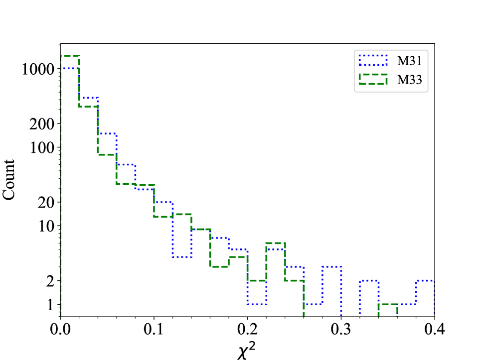
Figure 5: Distribution of $\chi^{2}$ of the model fitting for M31 (blue line) and M33 (green line).

The $\chi^{2}$ distribution is shown in Figure 5 after dropping 12 sources with $\chi^{2}>0.5$. The unsuccessful cases are mainly caused by photometric error. In addition the wrong cross-identification may be responsible for a few cases, and the light variation of RSGs may bring about the disparity between optical and infrared flux. Some RSGs have optically-thin shells with $\tau_{\mathrm{V}}<0.1$ that no discrimination can be made on dust species. For such sources, the amorphous silicate is assigned according to the cosmic abundance, and they constitute an “optically-thin” group to be treated separately. The sources with optical depth $\tau_{\mathrm{V}}\geq 0.1$ are divided into two groups by the dust species, either amorphous silicate or carbon determined by which yields the smaller $\chi^{2}$.

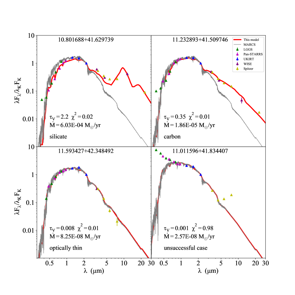
Figure 6: The examples of four typical dust model fittings (red line) to the spectral energy distributions, in a clockwise direction are the cases of amorphous silicate, amorphous carbon, optically thin and unsuccessful respectively. Also shown are the MARCS photospheric model spectrum (grey line), the photometric results from various surveys (triangles), the key model fitting parameters as well as the coordinate name of the source.

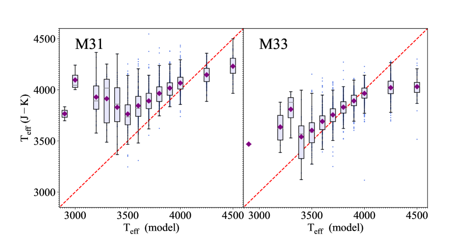
Figure 7: Comparison of the effective temperature derived from the model fitting and from the color index $J-K$.

Figure 6 displays the examples for four typical cases of circumstellar dust, i.e. amorphous silicate, amorphous carbon, optically thin, and one unsuccessful case. The parameter $T_{\rm{eff}}$ derived from the model fitting is compared with that from the color index $J-K$ (Equation 1) in Figure 7. Because the model grids provide only some discrete values, many sources have the same $T_{\rm{eff}}$, thus the mean and the standard deviation are marked. The agreement is very well at $T_{\rm{eff}}>$3400 K, while $T_{\rm{eff}}$ becomes smaller than that from $J-K$ at $T_{\rm{eff}}<$3400 K. This discrepancy may be attributed to replacing the massive star model by low-mass star model at low $T_{\rm{eff}}$, but might also be due to that Equation 1 to transform the color index to $T_{\rm{eff}}$ is not feasible at low $T_{\rm{eff}}$.

4 Result and discussion

4.1 Proportion of RSGs with silicate and carbon dust

The results of fitting are divided into three types according to the property of circumstellar dust, (1) silicate, (2) carbon and (3) optically thin with $\tau_{\mathrm{V}}<0.1$. In general, the silicate emission feature around 9.7$\mu$m leads to a relatively steep increase from the Spitzer/IRAC3 band at $\sim 5.8\mu$m to the IRAC4 band at $\sim 8.0\mu$m, while the carbonaceous dust produces a plateau-like shape from 3.5$\mu$m to 8$\mu$m. For the third type, the optical depth of the circumstellar shell is very small that the infrared SED can be almost described by the stellar model, consequently there is no significant difference in taking the amorphous silicate or carbon dust. Because RSGs are supposed to be O-rich in origin, we assign Type 3 objects to have silicate dust as Type 1.

The number of objects in each type is presented in Table 1. Among the 3712 (1733 + 1979 for M31 and M33 respectively) RSGs, 1665 (671 + 994) sources are best fitted by silicate dust, 581 sources (329 + 252) are attributed to amorphous carbon dust. This result means that 16% of RSGs have carbon-rich circumstellar dust on average, with 19% in M31 and 13% in M33. These percentages present the statistical study of the proportion of carbon-rich dust around RSGs for the first time. It may be argued that the SED of some assigned carbon-rich RSGs can also be fitted by silicate dust. This is true if the priority is not given to the smaller $\chi^{2}$ but to the silicate dust. On other hand, our fitting is neither skewed to carbon dust. The infrared spectroscopy of such as JWST would be very helpful to ascertain the chemical nature. Indeed, there have been other attempts to identify the carbon dust around RSGs from photometry. For example, Yang et al. (2018) attributed the difference in the mid-infrared colors related to the Spitzer and WISE bands to the PAH emission for the RSGs in the LMC. Basically, PAH is an indicator of carbonaceous environment. Interestingly, they found about 15% RSGs showing the evidence of PAH, this proportion coincides with the present work. Similarly, Yang et al. (2020) studied the SMC RSGs and also found the mid-infrared colors being an indicator of the PAH emission, but only 4% being so, much smaller than in the LMC.

In comparison, the ratio of carbon-rich to oxygen-rich AGB stars is found to be 0.53 by Humphreys (2010) or 0.62 in the inner 4kpc for NGC 6822 which translates into an iron abundance of [Fe/H] = $-1.29$ by Sibbons et al. (2012). It seems our derived portion of carbon-rich RSGs is not very exaggerated if compared with the AGB stars. However, the metallicity of RSGs in NGC 6822 is found to be [Z] $\sim-0.52$ by Patrick et al. (2015), which apparently differs from [Fe/H] = $-1.29$ derived from the C-/M-AGB ratio. RSGs and AGBs may be different populations due to the mass distinction. In spite that low- and intermediate-mass stars experience deep convection process that can dredge up the carbon element produced in helium burning to the surface to become carbon-rich, the mechanism for a RSG to become carbon-rich is lacking though convection exists at the surface of RSGs as well. The existence of carbon-rich RSGs is still puzzling.

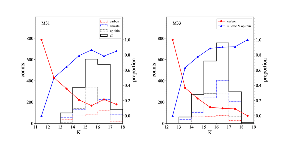
Figure 8: The change of carbon RSGs proportion with the $K$ magnitude, together with the histogram of RSGs with silicate and carbon dust respectively.

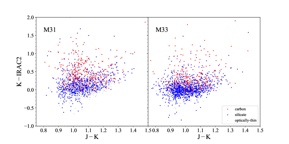
Figure 9: The $J-K/K-IRAC2$ diagram for RSGs with amorphous silicate, amorphous carbon dust as well as the optically thin sources.

The proportion of carbon dust RSG is found to increase with the brightness, as shown in Figure 8. Interestingly the brightest RSG in both M31 and M33 has a carbon dust shell. This may be accidental because the number of bright RSGs makes no statistical significance, thus the proportion for $K<13$ is unreliable. But the trend of increasing carbon dust with brightness continues for fainter RSG. In other words, the more massive RSGs may possess a carbon-rich dust shell more easily. In the color-color diagrams, Figure 9 and 10, the carbon dust is distinguishable from the silicate dust. The RSGs with carbon dust is on average redder in $K-IRAC2$. Previous works have noticed that this color index becomes negative at low temperature for RSGs (c.f. Yang et al. (2019)) which is believed due to the CO absorption in the $IRAC2$ band. The RSG with carbon dust yet has a positive value, indicating normal continuum emission of dust, which may imply that the CO band absorption can be neglected. On the contrary, the RSG with carbon dust is bluer in $K-IRAC4$. This can be understood if the carbon-rich dust brings about some PAH emission in the $IRAC4$ band, though the dust species used in the model fitting is amorphous carbon. The discrimination of carbon and silicate dust in these two color-color diagrams generally agree with our model fitting of the dust species. Nevertheless, there does exist some confusion in both diagrams, and no clear borderline can be recognized. Definitely, the SED of some RSGs cannot be explained by silicate dust and additional dust component must be supplemented, and at present carbonaceous dust seems to the only applicable. The percentage of carbon dust derived in this work still has some uncertainty, but this comes from the model fitting. In later analysis, we will divide the sample into carbon and silicate RSGs according to the model fitting results.

4.2 Mass Loss Rate

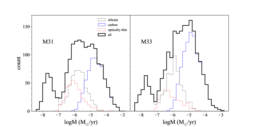
Figure 11: The distribution of mass loss rates for RSGs in M31 (left) and M33 (right).

The distribution of MLR is presented in Figure 11. The statistical properties are listed in Table 3, where all the values are calculated with a gas-to-dust ratio of 100 and the column “all” includes the optically thin sources. The MLR ranges from $10^{-9}$ to $10^{-3}{\text{M}_{\odot}}/{\rm yr}$, with a median value of $\sim 3.1\times 10^{-6}{\text{M}_{\odot}}/{\rm yr}$ that is an order-of-magnitude smaller than the mean value of ${\sim}2.0\times 10^{-5}{\text{M}_{\odot}}/{\rm yr}$, caused by numerous sources with very low MLR i.e. the optically thin sources. In general, the average MLR is about 16% higher in M33 than in M31. On the other hand, the summed MLR of the sample RSGs in M33 ($3.97\times 10^{-2}{\text{M}_{\odot}}/{\rm yr}$) is about 13% higher than in M31 ($3.51\times 10^{-2}{\text{M}_{\odot}}/{\rm yr}$). If the RSGs are divided into two groups according to the species of the circumstellar dust, some difference appears. The MLR is higher in case of silicate dust than of carbon dust on average, and the histogram shows clearly that the carbon dust sources lack very high MLR. In addition, the range of MLR in case of carbon dust is more concentrated. The reason may come from the difference in the dust property. As illustrated in Section 3.1, the parameter $\frac{a}{Q_{e}}$ is 1.573 and 0.263 for silicate and amorphous carbon respectively, to which the MLR is proportional. This implies that the MLR differs by a factor of six between silicate and carbon circumstellar shells even they have the same optical depth and inner dust radius. The density difference that $\rho_{\rm silicate}=3.5\text{g/cm}^{3}$ is 1.5 times $\rho_{\rm AC}=2.26\text{g/cm}^{3}$ yields even higher MLR in case of silicate dust. Apparently the higher-MLR RSGs with silicate dust need not be redder than those with carbon dust, which agrees with the observations.

Our results can be compared with the MLR of RSGs in previous works mentioned in Introduction. All the previous values of MLR lie apparently within the range of the present sample from $10^{-9}$ to $10^{-3}{\text{M}_{\odot}}/{\rm{yr}}$. The MLR of a few bright RSGs in the Milky Way from Gordon et al. (2018) as well as the dusty RSGs in the LMC from van Loon et al. (2005) is at the high-end of our sample, which can be understood either by their high luminosity or large optical depth. The large sample of AGB and RSG stars in the LMC from Riebel et al. (2012) exhibits a range of dust MLR between $10^{-7}$ to $10^{-11}{\text{M}_{\odot}}/{\rm yr}$, which coincides with our results as well if the gas-to-dust ratio of 400 is adopted. Generally our results support previous works with a much more complete sample that covers various cases of MLR of RSGs.

4.3 Relation of MLR with stellar luminosity

The relation of MLR with stellar parameters is widely calibrated, some of which is mentioned in Introduction. With the measured $J-K$, the effective temperature $T_{\rm{eff}}$ and the bolometric correction to the $K$ magnitude are calculated in Section 2.4. The linear relation is fitted between MLR and $\log L/{L_{\odot}}$. Excluding the optically thin RSGs, the relations are derived for silicate and amorphous carbon dust respectively:

$$\text{log}\dot{M}=0.83{\text{log}L/L_{\odot}}-8.31\text{\qquad forM31(silicate)}$$ (7)

$$\text{log}\dot{M}=0.91{\text{log}L/L_{\odot}}-10.03\text{\qquad forM31(carbon)}$$ (8)

$$\text{log}\dot{M}=0.92{\text{log}L/L_{\odot}}-8.64\text{\qquad forM33(silicate)}$$ (9)

$$\text{log}\dot{M}=1.14{\text{log}L/L_{\odot}}-11.13\text{\qquad forM33(carbon).}$$ (10)

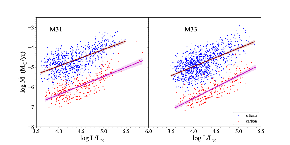
Figure 12: The relation of mass loss rate to the luminosity.

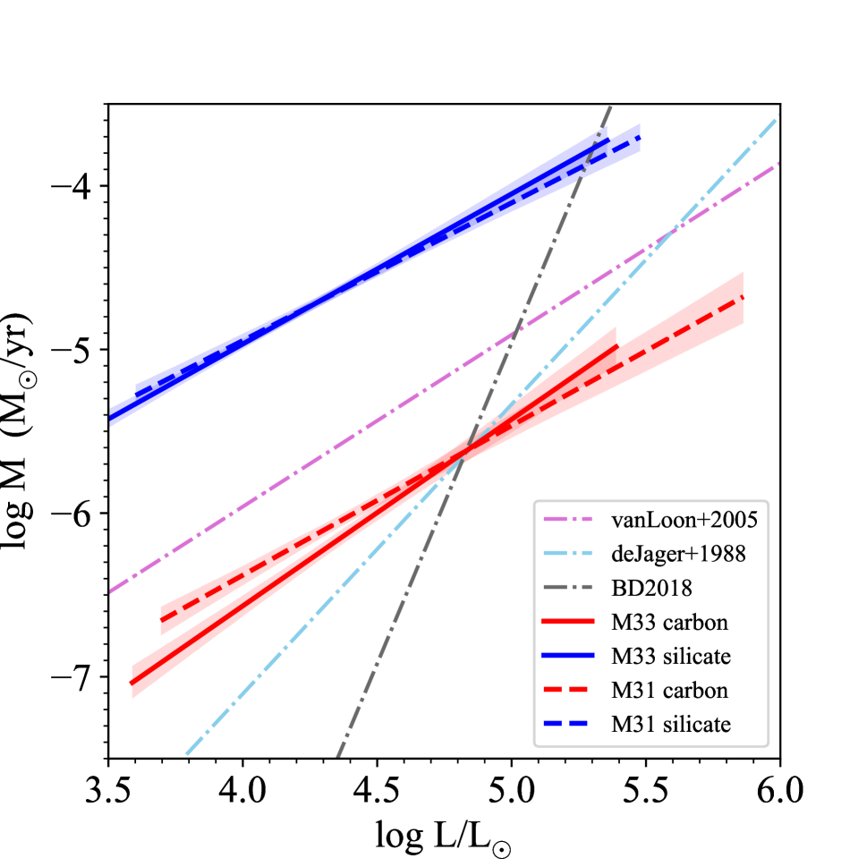
Figure 13: Comparison of the relation of mass loss rate to the luminosity with the works of de Jager et al. (1988), van Loon et al. (2005) and Beasor & Davies (2018).

Table 3 shows that the correlation is moderate. The results are displayed in Figure 12, and compared with previous results in Figure 13. The slope, i.e. the power law index $\gamma$ in the relation of $\dot{M}\propto L^{\gamma}$, is unanimous in various cases, i.e. unanimous in M31 and M33, and unanimous for silicate and carbon dust. This index also agrees with that from van Loon et al. (2005) and de Jager et al. (1988) for dusty RSGs in the LMC. It should be mentioned that, van Loon et al. (2005) and de Jager et al. (1988) actually derive the relations of MLR with not only luminosity but also effective temperature, and the $\dot{M}-L$ relation displayed in Figure 12 is calculated with a mean effective temperature of our sample at 3921K. In addition, this index is around 1.0, which means that MLR is approximately proportional to luminosity. On the other hand, the index is apparently smaller than that from Beasor & Davies (2018) for RSGs in the Galactic clusters. The discrepancy of Beasor & Davies (2018) with others may be caused by that their sample is different, and that they adopted a gas-to-dust ratio of 200.

Different from the unanimous slope, the intercept, i.e. the proportional coefficient of the $\dot{M}\propto L^{\gamma}$ relation, is not unanimous. As discussed in Section 3.1, the amount of MLR depends on multiple factors, including the dust species, the dust size, the stellar expansion velocity and luminosity. The effects of dust species and size are discussed in previous sections, which can be as large as one order of magnitude. The expansion velocity and luminosity should have less effect, probably change the MLR by a few times. Taking all the factors into account, the MLR may differ by two orders of magnitude for a given observational SED, therefore the comparison of the vertical shift is meaningful only under the same model conditions.

Taking $T_{\text{eff}}$ into account, the relationships become:

$$\text{log}\dot{M}=0.82{\text{log}L/L_{\odot}}-0.90\text{log}T_{\text{eff}}-4.95\text{\qquad forM31(silicate)}$$ (11)

$$\text{log}\dot{M}=0.89{\text{log}L/L_{\odot}}-0.68\text{log}T_{\text{eff}}-7.49\text{\qquad forM31(carbon)}$$ (12)

$$\text{log}\dot{M}=0.73{\text{log}L/L_{\odot}}-4.84\text{log}T_{\text{eff}}-9.51\text{\qquad forM33(silicate)}$$ (13)

$$\text{log}\dot{M}=1.02{\text{log}L/L_{\odot}}-3.49\text{log}T_{\text{eff}}+1.87\text{\qquad forM33(carbon).}$$ (14)

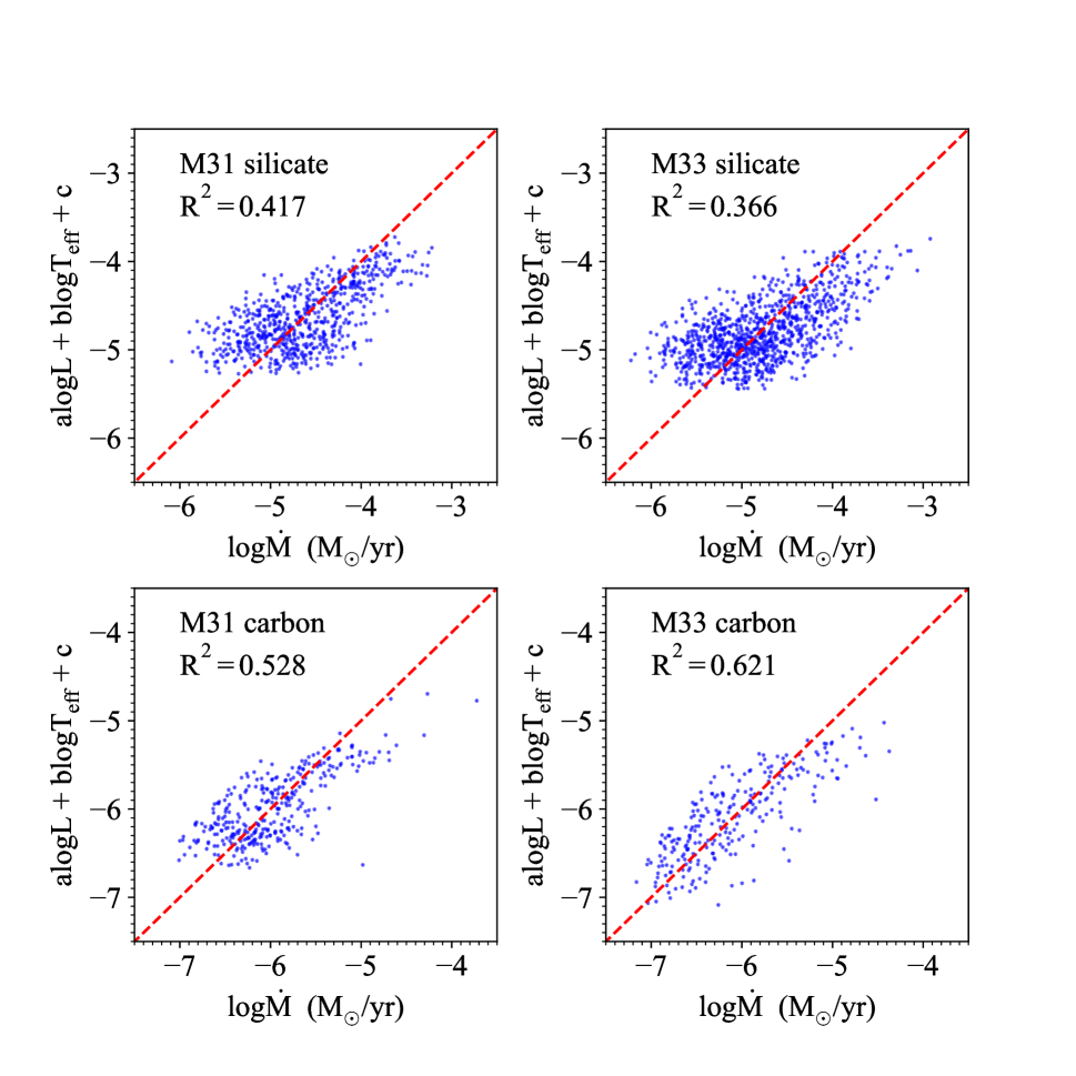
Figure 14: The relation of mass loss rate with the luminosity and the effective temperature, and the red line marks $Y=X$.

The fitting results are displayed in Figure 14 with the value of $R^{2}$ which implies an improved relation in comparison with the luminosity alone. In general, the fitting is reasonably well with the residual $|\log\dot{M}_{\rm predict}-\log\dot{M}|<1.0$, meanwhile it deviates somehow from the measurements in particular for the silicate dust. This may be understood that MLR depends on other parameters in addition to $L$ and $T_{\rm eff}$, such as stellar mass, radius or surface gravity (Reimers, 1975; Beasor et al., 2020), and pulsation period (Goldman et al., 2017). But these parameters are not conveniently available from observation.

4.4 Relation of MLR with infrared brightness

After examining the infrared-band brightness, a very good relation is found with the mid-infrared flux in the Spitzer/IRAC4 band at 8$\mu$m and the MIPS24 band at 24$\mu$m. The linear fitting yields the following relations with the absolute magnitude for which the distance modulus is 24.32 and 24.50 (Paper I) for M31 and M33 respectively.

$$\text{log}\dot{M}=-0.46{M_{\rm IRAC4}}-9.37\text{\qquad forM31(silicate)}$$ (15)

$$\text{log}\dot{M}=-0.36{M_{\rm IRAC4}}-9.57\text{\qquad forM31(carbon)}$$ (16)

$$\text{log}\dot{M}=-0.47{M_{\rm IRAC4}}-9.58\text{\qquad forM33(silicate)}$$ (17)

$$\text{log}\dot{M}=-0.42{M_{\rm IRAC4}}-10.31\text{\qquad forM33(carbon)}$$ (18)

$$\text{log}\dot{M}=-0.38{M_{\rm MIPS24}}-9.48\text{\qquad forM31(silicate)}$$ (19)

$$\text{log}\dot{M}=-0.37{M_{\rm MIPS24}}-10.48\text{\qquad forM31(carbon)}$$ (20)

$$\text{log}\dot{M}=-0.38{M_{\rm MIPS24}}-9.68\text{\qquad forM33(silicate)}$$ (21)

$$\text{log}\dot{M}=-0.43{M_{\rm MIPS24}}-11.41\text{\qquad forM33(carbon)}$$ (22)

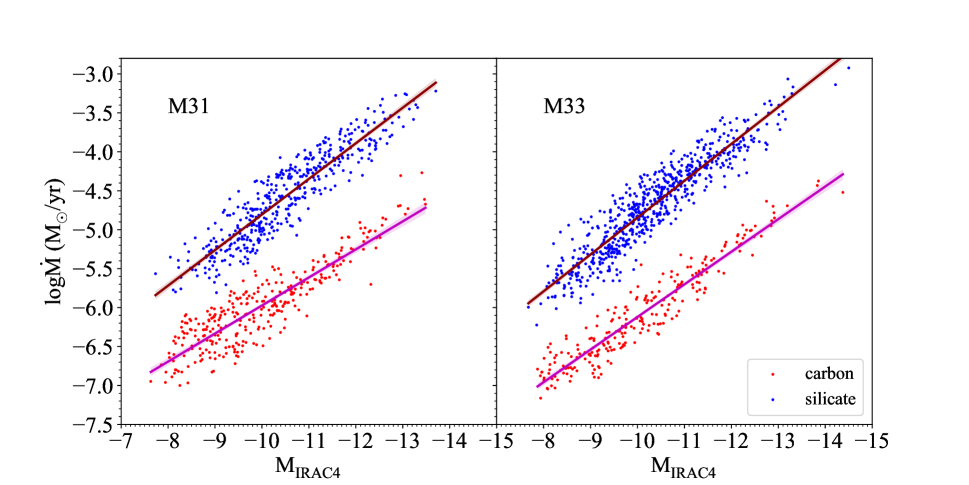
Figure 15: The relation of mass loss rate to the Spitzer/IRAC4 absolute magnitude.

The fitting lines are shown in Figure 15 and 16. The correlation coefficients are all large ($<-0.7$) listed in Table 3, which implies a tight relation of the mid-infrared flux with the MLR. This relation is expected from the warm temperature of the circumstellar dust which emits mainly in the mid-infrared. On other hand, the relation with near-infrared flux is weak and not presented.

4.5 Relation of MLR with infrared color indexes

Examining the infrared colors, it is found that the MLR is sensitive to $IRAC1-IRAC4$:

$$\text{log}\dot{M}=0.24(m_{\rm IRAC1}-m_{\rm IRAC4})-4.86\text{\qquad forM31(silicate)}$$ (23)

$$\text{log}\dot{M}=0.46(m_{\rm IRAC1}-m_{\rm IRAC4})-6.25\text{\qquad forM31(carbon)}$$ (24)

$$\text{log}\dot{M}=0.34(m_{\rm IRAC1}-m_{\rm IRAC4})-5.18\text{\qquad forM33(silicate)}$$ (25)

$$\text{log}\dot{M}=0.64(m_{\rm IRAC1}-m_{\rm IRAC4})-6.50\text{\qquad forM33(carbon)}$$ (26)

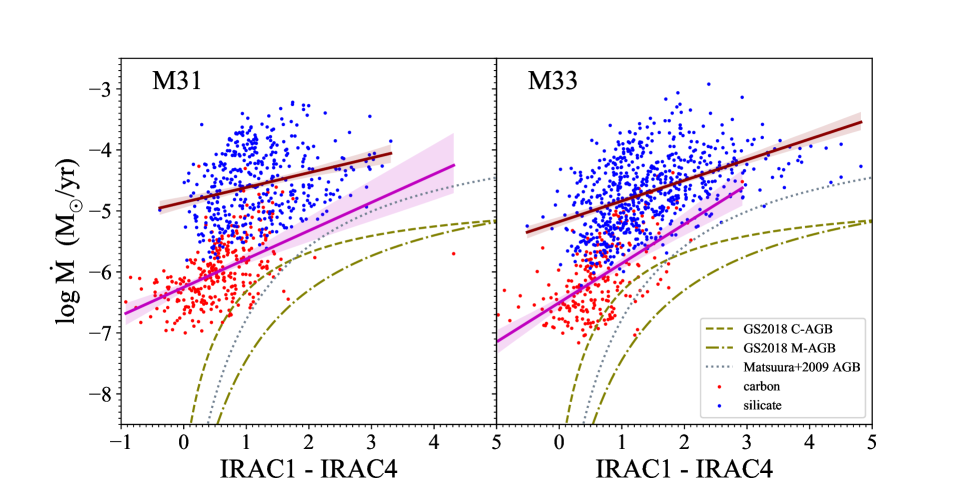
Figure 17: The relation of mass loss rate to the color index $IRAC1-IRAC4$, which is compared with that from Groenewegen & Sloan (2018) and Matsuura et al. (2009).

As seen in Figure 17, the scattering around the fitting line is significant, and the correlation of MLR with the color index is not so tight as with the mid-infrared flux. The correlation coefficients in Table 3 also manifest that the correlation is very weak for silicate dust, and moderate for carbon dust. Previously, Groenewegen & Sloan (2018) and Matsuura et al. (2009) derived the relation of MLR with $IRAC1-IRAC4$ as well for AGB stars, but they take an exponential function as illustrated in Figure 17 by the dash-dot lines which hardly delineate the tendency for the RSGs sample. It seems no good relation exists for the MLR with the infrared colors.

4.6 Total mass loss rate

The initial sample from Paper I should be complete since the lower limit of the RSG brightness in M31 and M33 is higher than the observational complete magnitude. But the sample for which we derived the MLR is incomplete after removing those without appropriate photometric SED. Nevertheless, the comparison with the initial sample shown in Figure 1 finds no bias to the $K$ magnitude or the $J-K$ colors. Thus we simply multiply the summed MLR from our sample by the ratio of the initial sample to the final sample, i.e. $5253/1733=3.03$ for M31 and $3001/1979=1.52$ for M33. As listed in Table 2, the summed mass loss rate of all the modelled sample RSGs in M31 is $\sim 0.035{\text{M}_{\odot}}/\text{yr}$, and in M33 is $\sim 0.040{\text{M}_{\odot}}/\text{yr}$. After multiplying by this ratio, the total MLR of RSG is then $0.11{\text{M}_{\odot}}/\text{yr}$ in M31 and $0.060{\text{M}_{\odot}}/\text{yr}$ in M33. Dividing by the gas-to-dust ratio, i.e. 100 in this work, the dust production rate by RSGs is $10^{-3}{\text{M}_{\odot}}/\text{yr}$ in M31 and $6\times 10^{-4}{\text{M}_{\odot}}/\text{yr}$ in M33. At present, we have no idea on the dust mass contributed by AGB stars in M31 or M33. Taking the Milky Way galaxy as a reference, the dust production rate by evolved low mass stars is a few $10^{-3}{\text{M}_{\odot}}/\text{yr}$ according to Draine (2009), or about $10^{-3}{\text{M}_{\odot}}/\text{yr}$ according to Jones (2001). Though the uncertainty of these values may be a few factors, it seems that RSGs can be a non-negligible source of interstellar dust. The precise estimation of the portion of RSGs dust can be made only after a systematic calculation of the MLR of AGB stars in M31 and M33 in our further work.

4.7 Influence of metallicity and surface gravity

Metallicity and surface gravity change the stellar spectrum as well as effective temperature, which are assumed to be constant in modelling. The metallicity of both M31 (Blair et al., 1982) and M33 (U et al., 2009) is found to exhibit some gradient with the distance from the center. Considering that RSGs are located in the spiral arm or ring area, the case of [Z] = 0.25 with the MARCS RSGs model is examined. Although (Goldman et al., 2017) derived a relation of the wind speed proportional to metallictiy, a scale of [Z] = 0.25 would yield an unreasonably high expansion velocity. Moreover, they suggest that the mass-loss rate is independent of metallicity between a half and twice solar. Thus the velocity is still calculated with [Z]=0. The resultant MLR is listed in Table 6. It can been seen that a higher metallicity will bring about a higher MLR, which is possibly caused by a lower bump in the $J,H,K$ bands.

Quantitatively, the mean MLR shows very little difference when [Z] changes from 0 to 0.25, with a number of $2.03\times 10^{-5}{\text{M}_{\odot}}/\text{yr}$ meaning an increase of 1%. For the surface gravity, the case of $\log g=-0.5$ is examined. As shown in Table 6, the mean MLR increases to $2.03\times 10^{-5}{\text{M}_{\odot}}/\text{yr}$ with $\log g=-0.5$, i.e. 1%. To sum up, the influence of stellar metallicity and surface gravity is very small, only about one percent.

Figure 1: The initial (grey dots) and final (red dots) sample of RSGs in the $J-K/K$ diagram for M31 as well as the histogram of $J-K$ and $K$. Also plotted is the density contour of RGB and AGB stars for reference.

Figure 2: The RSGs in the $J-K/K$ diagram for M33, the symbols are the same as in Figure 1.

Figure 3: The $A_{V}$ distribution of RSGs in M31 and M33.

Figure 4: The change of the extinction coefficient $Q_{e}$ (left) and the ratio $a/Q_{e}$ (right) in the $V$ band with the radius of the dust grain $a$ for three dust species, i.e. amorphous silicate from DL84, amorphous carbon from RM91 and HN88 respectively. The inset shows the value of $a/Q_{e}$ for an MRN size distribution adopted in this work, and for a unique radius of $a=0.1\mu$m and $a=0.3\mu$m used in previous works.

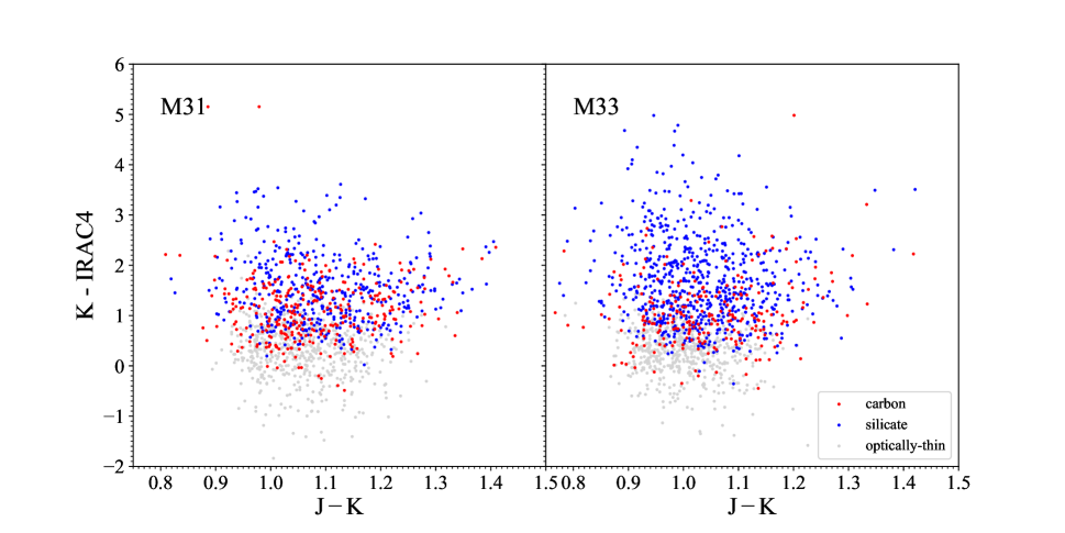
Figure 10: The $J-K/K-IRAC4$ diagram for RSGs with amorphous silicate, amorphous carbon dust as well as the optically thin sources.

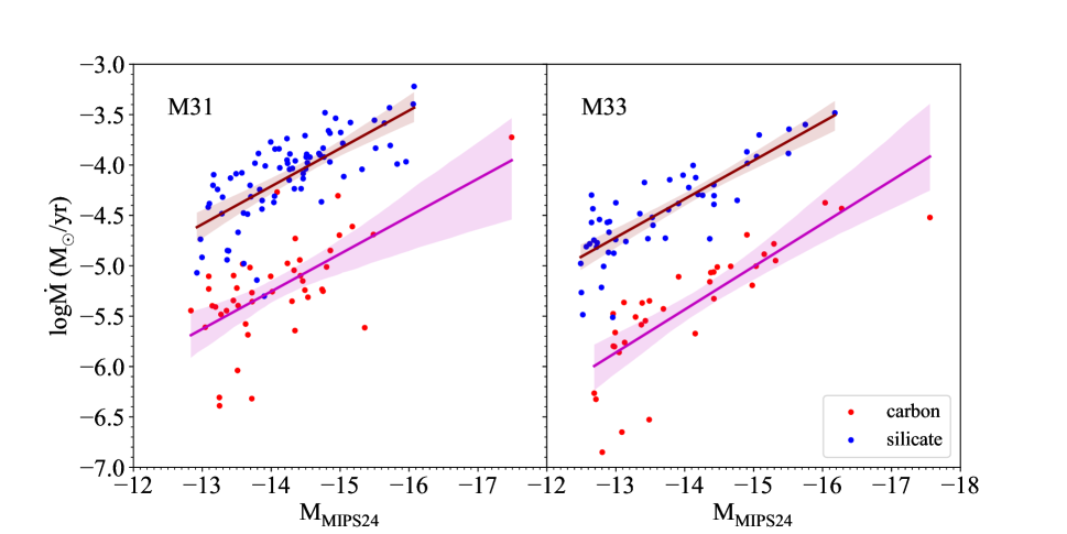
Figure 16: The relation of mass loss rate to the Spitzer/MIPS24 absolute magnitude.

Table 1: Number of RSGs in M31 and M33

	M31+M33	M31	M33
Paper I	8254	5253	3001
sample	3712	1733	1979
carbon	581	329	252
silicate	1665	671	994
op-thin	1466	733	733
Carbon%	16%	19%	13%
Op-thin%	39%	42%	37%

Table 2: Mass loss rates of RSGs in M31 and M33 (M_⊙/yr)

	M31			M33
	carbon	silicate	all	carbon	silicate	all
mean	2.92E-06	4.86E-05	2.02E-05	2.34E-06	3.82E-05	2.01E-05
median	8.92E-07	2.11E-05	2.66E-06	6.13E-07	1.49E-05	3.45E-06
min	9.80E-08	8.14E-07	4.29E-09	6.87E-08	5.97E-07	3.54E-09
max	1.88E-04	6.03E-04	6.03E-04	4.22E-05	1.20E-03	1.20E-03
sum	9.59E-04	3.26E-02	3.51E-02	5.91E-04	3.80E-02	3.97E-02

Table 3: The Spearman’s rank correlation coefficient of the logarithmic mass loss rate with stellar luminosity, infrared magnitude and colors

	M31		M33
	silicate	carbon	silicate	carbon
log$L$	0.59	0.66	0.54	0.78
$M_{\rm IRAC4}$	-0.92	-0.86	-0.93	-0.94
$M_{\rm MIPS24}$	-0.76	-0.56	-0.80	-0.90
IRAC1-IRAC4	0.29	0.57	0.50	0.56

Table 4: Catalog of the stellar and dust parameters for red supergiants in M31

index	RA	DEC	galaxy	KMag	$\rm KMag\_{Err}$	log$L/L_{\odot}$	$T_{\rm eff}$	$\dot{M}$	$T_{\rm in}$	$\tau_{V}$	$\chi^{2}$	type
	(deg)	(deg)		(mag)	(mag)		(K)	($M_{\odot}$/yr)	(K)
0	11.446398	42.345503	M31	15.689	0.010	4.312	3880	6.90E-07	1200	0.04	0.009	op-thin
1	11.469417	42.345959	M31	14.077	0.010	4.862	3564	9.02E-06	750	0.45	0.016	carbon
2	11.518298	42.411805	M31	15.118	0.010	4.506	3762	2.66E-06	900	0.05	0.007	op-thin
3	11.534664	42.378428	M31	15.780	0.010	4.227	3715	1.53E-07	1200	0.1	0.011	carbon
4	11.559090	42.317375	M31	17.179	0.028	3.780	4078	4.04E-06	750	0.3	0.015	silicate

Note. — (This table is available in its entirety in machine-readable form.)

Table 5: Catalog of the stellar and dust parameters for red supergiants in M33

index	RA	DEC	galaxy	KMag	$\rm KMag\_{Err}$	log$L/L_{\odot}$	$T_{\rm eff}$	$\dot{M}$	$T_{\rm in}$	$\tau_{V}$	$\chi^{2}$	type
	(deg)	(deg)		(mag)	(mag)		(K)	($M_{\odot}$/yr)	(K)
1733	23.222635	30.173420	M33	18.085	0.081	3.502	4144	9.18E-06	750	1.05	0.015	silicate
1734	23.202302	30.172458	M33	16.809	0.026	3.962	3976	2.64E-05	750	1.15	0.011	silicate
1735	23.643000	30.440888	M33	13.636	0.010	5.057	3405	1.04E-04	1200	1.3	0.016	silicate
1736	23.660640	30.439871	M33	17.223	0.028	3.835	4108	2.44E-05	750	1.35	0.015	silicate
1737	23.551408	30.436721	M33	16.008	0.010	4.246	3861	3.49E-07	1050	0.15	0.009	carbon

Note. — (This table is available in its entirety in machine-readable form.)

Table 6: The effect of metallicity and surface gravity on the mass loss rate

	[Z]	$\log g$	$\Sigma{\chi^{2}}$	mean $\dot{M}$	median $\dot{M}$	optically-thin sources
				(M⊙/yr)	(M⊙/yr)	Number
This Model	0	0	93.9	2.01E-5	3.08E-6	1466
$\log g$=-0.5	0	-0.5	101.4	2.03E-5	3.14E-6	1436
$[Z]=0.25$	0.25	0	102.7	2.03E-5	3.27E-6	1375

References

- Astropy Collaboration et al. (2013) Astropy Collaboration, Robitaille, T. P., Tollerud, E. J., et al. 2013, A&A, 558, A33, doi: 10.1051/0004-6361/201322068
- Beasor & Davies (2018) Beasor, E. R., & Davies, B. 2018, MNRAS, 475, 55, doi: 10.1093/mnras/stx3174
- Beasor et al. (2020) Beasor, E. R., Davies, B., Smith, N., et al. 2020, MNRAS, 492, 5994, doi: 10.1093/mnras/staa255
- Bianchi et al. (1996) Bianchi, L., Clayton, G. C., Bohlin, R. C., Hutchings, J. B., & Massey, P. 1996, ApJ, 471, 203, doi: 10.1086/177963
- Blair et al. (1982) Blair, W. P., Kirshner, R. P., & Chevalier, R. A. 1982, ApJ, 254, 50, doi: 10.1086/159703
- Cardelli et al. (1989) Cardelli, J. A., Clayton, G. C., & Mathis, J. S. 1989, ApJ, 345, 245, doi: 10.1086/167900
- Chambers et al. (2016) Chambers, K. C., Magnier, E. A., Metcalfe, N., et al. 2016, The Pan-STARRS1 Surveys. https://arxiv.org/abs/1612.05560
- Cox et al. (2012) Cox, N. L. J., Kerschbaum, F., van Marle, A. J., et al. 2012, A&A, 537, A35, doi: 10.1051/0004-6361/201117910
- De Beck et al. (2010) De Beck, E., Decin, L., de Koter, A., et al. 2010, A&A, 523, A18, doi: 10.1051/0004-6361/200913771
- de Jager et al. (1988) de Jager, C., Nieuwenhuijzen, H., & van der Hucht, K. A. 1988, A&AS, 72, 259
- Draine (2009) Draine, B. T. 2009, in Astronomical Society of the Pacific Conference Series, Vol. 414, Cosmic Dust - Near and Far, ed. T. Henning, E. Grün, & J. Steinacker, 453. https://arxiv.org/abs/0903.1658
- Draine & Lee (1984) Draine, B. T., & Lee, H. M. 1984, ApJ, 285, 89, doi: 10.1086/162480
- Ekström et al. (2013) Ekström, S., Georgy, C., Meynet, G., Groh, J., & Granada, A. 2013, in EAS Publications Series, Vol. 60, EAS Publications Series, ed. P. Kervella, T. Le Bertre, & G. Perrin, 31–41, doi: 10.1051/eas/1360003
- Gail & Sedlmayr (1984) Gail, H. P., & Sedlmayr, E. 1984, A&A, 132, 163
- Gail & Sedlmayr (1999) —. 1999, A&A, 347, 594
- Goldman et al. (2017) Goldman, S. R., van Loon, J. T., Zijlstra, A. A., et al. 2017, MNRAS, 465, 403, doi: 10.1093/mnras/stw2708
- Gordon et al. (2016) Gordon, M. S., Humphreys, R. M., & Jones, T. J. 2016, ApJ, 825, 50, doi: 10.3847/0004-637X/825/1/50
- Gordon et al. (2018) Gordon, M. S., Humphreys, R. M., Jones, T. J., et al. 2018, AJ, 155, 212, doi: 10.3847/1538-3881/aab961
- Groenewegen (2012) Groenewegen, M. A. T. 2012, A&A, 543, A36, doi: 10.1051/0004-6361/201218965
- Groenewegen et al. (2002) Groenewegen, M. A. T., Sevenster, M., Spoon, H. W. W., & Pérez, I. 2002, A&A, 390, 511, doi: 10.1051/0004-6361:20020728
- Groenewegen & Sloan (2018) Groenewegen, M. A. T., & Sloan, G. C. 2018, A&A, 609, A114, doi: 10.1051/0004-6361/201731089
- Gustafsson et al. (2008) Gustafsson, B., Edvardsson, B., Eriksson, K., et al. 2008, A&A, 486, 951, doi: 10.1051/0004-6361:200809724
- Hanner (1988) Hanner, M. 1988, Grain optical properties., Infrared Observations of Comets Halley and Wilson and Properties of the Grains
- Humphreys (2010) Humphreys, R. M. 2010, in Astronomical Society of the Pacific Conference Series, Vol. 425, Hot and Cool: Bridging Gaps in Massive Star Evolution, ed. C. Leitherer, P. D. Bennett, P. W. Morris, & J. T. Van Loon, 247
- Hyland et al. (1969) Hyland, A. R., Becklin, E. E., Neugebauer, G., & Wallerstein, G. 1969, ApJ, 158, 619, doi: 10.1086/150224
- Ivezic & Elitzur (1997) Ivezic, Z., & Elitzur, M. 1997, MNRAS, 287, 799, doi: 10.1093/mnras/287.4.799
- Johnson (1968) Johnson, H. L. 1968, ApJ, 154, L125, doi: 10.1086/180284
- Jones (2001) Jones, A. P. 2001, Philosophical Transactions of the Royal Society of London Series A, 359, 1961, doi: 10.1098/rsta.2001.0890
- Kudritzki & Reimers (1978) Kudritzki, R. P., & Reimers, D. 1978, A&A, 70, 227
- Levesque (2010) Levesque, E. M. 2010, New Astronomy Reviews, 54, 1, doi: https://doi.org/10.1016/j.newar.2009.10.002
- Liu & Jiang (2017) Liu, J., & Jiang, B. 2017, AJ, 153, 176, doi: 10.3847/1538-3881/aa6334
- Massey & Evans (2016) Massey, P., & Evans, K. A. 2016, The Astrophysical Journal, 826, 224
- Massey et al. (2007) Massey, P., Olsen, K. A. G., Hodge, P. W., et al. 2007, AJ, 133, 2393, doi: 10.1086/513319
- Massey et al. (2006) —. 2006, AJ, 131, 2478, doi: 10.1086/503256
- Massey et al. (2005) Massey, P., Plez, B., Levesque, E. M., et al. 2005, ApJ, 634, 1286, doi: 10.1086/497065
- Matsuura et al. (2009) Matsuura, M., Barlow, M. J., Zijlstra, A. A., et al. 2009, MNRAS, 396, 918, doi: 10.1111/j.1365-2966.2009.14743.x
- Meynet et al. (2015) Meynet, G., Chomienne, V., Ekström, S., et al. 2015, A&A, 575, A60, doi: 10.1051/0004-6361/201424671
- Neugent et al. (2020) Neugent, K. F., Massey, P., Georgy, C., et al. 2020, ApJ, 889, 44, doi: 10.3847/1538-4357/ab5ba0
- Ohnaka et al. (2008) Ohnaka, K., Izumiura, H., Leinert, C., et al. 2008, A&A, 490, 173, doi: 10.1051/0004-6361:200810229
- Patrick et al. (2015) Patrick, L. R., Evans, C. J., Davies, B., et al. 2015, ApJ, 803, 14, doi: 10.1088/0004-637X/803/1/14
- Ramstedt et al. (2006) Ramstedt, S., Schöier, F. L., Olofsson, H., & Lundgren, A. A. 2006, A&A, 454, L103, doi: 10.1051/0004-6361:20065285
- Reimers (1975) Reimers, D. 1975, Memoires of the Societe Royale des Sciences de Liege, 8, 369
- Ren et al. (2021) Ren, Y., Jiang, B., Yang, M., et al. 2021, The Astrophysical Journal, 907, 18, doi: 10.3847/1538-4357/abcda5
- Riebel et al. (2012) Riebel, D., Srinivasan, S., Sargent, B., & Meixner, M. 2012, ApJ, 753, 71, doi: 10.1088/0004-637X/753/1/71
- Rieke et al. (2004) Rieke, G. H., Young, E. T., Engelbracht, C. W., et al. 2004, ApJS, 154, 25, doi: 10.1086/422717
- Rouleau & Martin (1991) Rouleau, F., & Martin, P. G. 1991, ApJ, 377, 526, doi: 10.1086/170382
- Sargent et al. (2010) Sargent, B. A., Srinivasan, S., Meixner, M., et al. 2010, ApJ, 716, 878, doi: 10.1088/0004-637X/716/1/878
- Schlegel et al. (1998) Schlegel, D. J., Finkbeiner, D. P., & Davis, M. 1998, ApJ, 500, 525, doi: 10.1086/305772
- Scicluna et al. (2015) Scicluna, P., Siebenmorgen, R., Wesson, R., et al. 2015, A&A, 584, L10, doi: 10.1051/0004-6361/201527563
- Sibbons et al. (2012) Sibbons, L. F., Ryan, S. G., Cioni, M. R. L., Irwin, M., & Napiwotzki, R. 2012, A&A, 540, A135, doi: 10.1051/0004-6361/201118365
- Smartt (2009) Smartt, S. J. 2009, ARA&A, 47, 63, doi: 10.1146/annurev-astro-082708-101737
- Srinivasan et al. (2011) Srinivasan, S., Sargent, B. A., & Meixner, M. 2011, A&A, 532, A54, doi: 10.1051/0004-6361/201117033
- Sylvester et al. (1998) Sylvester, R. J., Skinner, C. J., & Barlow, M. J. 1998, MNRAS, 301, 1083, doi: 10.1046/j.1365-8711.1998.02078.x
- Taylor (2005) Taylor, M. B. 2005, in Astronomical Society of the Pacific Conference Series, Vol. 347, Astronomical Data Analysis Software and Systems XIV, ed. P. Shopbell, M. Britton, & R. Ebert, 29
- U et al. (2009) U, V., Urbaneja, M. A., Kudritzki, R.-P., et al. 2009, ApJ, 704, 1120, doi: 10.1088/0004-637X/704/2/1120
- Ueta & Meixner (2003) Ueta, T., & Meixner, M. 2003, ApJ, 586, 1338, doi: 10.1086/367818
- van Loon et al. (2005) van Loon, J. T., Cioni, M. R. L., Zijlstra, A. A., & Loup, C. 2005, A&A, 438, 273, doi: 10.1051/0004-6361:20042555
- Verhoelst et al. (2009) Verhoelst, T., van der Zypen, N., Hony, S., et al. 2009, A&A, 498, 127, doi: 10.1051/0004-6361/20079063
- Wang & Chen (2019) Wang, S., & Chen, X. 2019, ApJ, 877, 116, doi: 10.3847/1538-4357/ab1c61
- Werner et al. (2004) Werner, M. W., Roellig, T. L., Low, F. J., et al. 2004, ApJS, 154, 1, doi: 10.1086/422992
- Wright et al. (2010) Wright, E. L., Eisenhardt, P. R. M., Mainzer, A. K., et al. 2010, AJ, 140, 1868, doi: 10.1088/0004-6256/140/6/1868
- Xue et al. (2016) Xue, M., Jiang, B. W., Gao, J., et al. 2016, ApJS, 224, 23, doi: 10.3847/0067-0049/224/2/23
- Yang et al. (2018) Yang, M., Bonanos, A. Z., Jiang, B.-W., et al. 2018, A&A, 616, A175, doi: 10.1051/0004-6361/201832833
- Yang et al. (2019) —. 2019, A&A, 629, A91, doi: 10.1051/0004-6361/201935916
- Yang et al. (2020) —. 2020, A&A, 639, A116, doi: 10.1051/0004-6361/201937168