Practical Relative Order Attack in Deep Ranking

Abstract

Recent studies unveil the vulnerabilities of deep ranking models, where an imperceptible perturbation can trigger dramatic changes in the ranking result. While previous attempts focus on manipulating absolute ranks of certain candidates, the possibility of adjusting their relative order remains under-explored. In this paper, we formulate a new adversarial attack against deep ranking systems, i.e., the Order Attack, which covertly alters the relative order among a selected set of candidates according to an attacker-specified permutation, with limited interference to other unrelated candidates. Specifically, it is formulated as a triplet-style loss imposing an inequality chain reflecting the specified permutation. However, direct optimization of such white-box objective is infeasible in a real-world attack scenario due to various black-box limitations. To cope with them, we propose a Short-range Ranking Correlation metric as a surrogate objective for black-box Order Attack to approximate the white-box method. The Order Attack is evaluated on the Fashion-MNIST and Stanford-Online-Products datasets under both white-box and black-box threat models. The black-box attack is also successfully implemented on a major e-commerce platform. Comprehensive experimental evaluations demonstrate the effectiveness of the proposed methods, revealing a new type of ranking model vulnerability.

1 Introduction

Thanks to the widespread applications of deep neural networks [27, 21] in the learning-to-rank tasks [52, 42], deep ranking algorithms have witnessed significant progress, but unfortunately they have also inherited the long-standing adversarial vulnerabilities [47] of neural networks. Considering the “search by image” application for example, an imperceptible adversarial perturbation to the query image is sufficient to intentionally alter the ranking results of candidate images. Typically, such adversarial examples can be designed to cause the ranking model to “misrank” [33, 30] (i.e., rank items incorrectly), or purposefully raise or lower the ranks of selected candidates  [60].

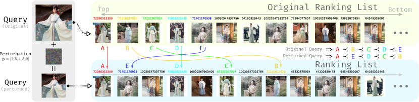
Figure 1: Showcase of a practical Order Attack (OA) against “JD SnapShop”, a major online retailing e-commerce platform. The query image is “Han Chinese clothing”. Numbers atop candidate images are Stock Keep Unit (SKU) IDs.

Since “misranking” can be interpreted as deliberately lowering the ranks of well-matching candidates, previous attacks on ranking models unanimously focus on changing the absolute ranks of a set of candidates, while neglecting the manipulation of relative order among them. However, an altered relative order can be disruptive in some applications, such as impacting sales on e-commerce platforms powered by content-based image retrieval [45], where potential customers attempt to find merchandise via image search.

As shown in Fig. 1, an attacker may want to adversarially perturb the query image and thus change the relative order among products A, B, C, D, and E into $\text{A}\prec\text{E}\prec\text{D}\prec\text{C}\prec\text{B}$ in the search-by-image result. The sales of a product closely correlates to its Click-Through Rate (CTR), while the CTR can be significantly influenced by its ranking position [10, 39] (which also decides the product pagination on the client side). Hence, subtle changes in the relative order of searches can be sufficient to alter CTR and impact the actual and relative sales among A to E.

Such vulnerability in a commercial platform may be exploited in a malfeasant business competition among the top-ranked products, e.g., via promoting fraudulent web pages containing adversarial example product images generated in advance. Specifically, the attack of changing relative order does not aim to incur significant changes in the absolute ranks of the selected candidates (e.g., moving from list bottom to top), but it intentionally changes the relative order of them subtly without introducing conspicuous abnormality. Whereas such goal cannot be implemented by absolute rank attacks such as [60], the relative order vulnerability may justify and motivate a more robust and fair ranking model.

Specifically, we propose the Order Attack (OA), a new adversarial attack problem in deep ranking. Given a query image ${\bm{q}}\in[0,1]^{D}$, a set of selected candidates ${\mathbb{C}}=\{{\bm{c}}_{1},{\bm{c}}_{2},\ldots,{\bm{c}}_{k}\}$, and a predefined permutation vector ${\mathbf{p}}=[p_{1},p_{2},\ldots,p_{k}]$, Order Attack aims to find an imperceptible perturbation ${\bm{r}}$ ($\|{\bm{r}}\|_{\infty}\leqslant\varepsilon$ and $\tilde{{\bm{q}}}={\bm{q}}+{\bm{r}}\in[0,1]^{D}$), so that $\tilde{{\bm{q}}}$ as the adversarial query can convert the relative order of the selected candidates into ${\bm{c}}_{p_{1}}\prec{\bm{c}}_{p_{2}}\prec\cdots\prec{\bm{c}}_{p_{k}}$. For example, a successful OA with ${\mathbf{p}}=[1,5,4,3,2]$ will result in ${\bm{c}}_{1}\prec{\bm{c}}_{5}\prec{\bm{c}}_{4}\prec{\bm{c}}_{3}\prec{\bm{c}}_{2}$, as shown in Fig. 1.

To implement OA, we first assume the white-box threat model (i.e., the ranking model details, incl. the gradient are accessible to the attacker). Recall that a conventional deep ranking model [52, 59, 42, 26] maps the query and candidates onto a common embedding space, and determines the ranking list according to the pairwise similarity between the query and these candidates. Thus, OA can be formulated as the optimization of a triplet-style loss function based on the inequality chain representing the desired relative order, which simultaneously adjusts the similarity scores between the query and the selected candidates. Additionally, a semantics-preserving penalty term [60] is also included to limit conspicuous changes in ranking positions. Finally, the overall loss function can be optimized with gradient methods such as PGD [34] to find the adversarial example.

However, in a real-world black-box attack scenario, practical limitations (e.g., gradient inaccessibility) invalidate the proposed method. To accommodate them and make OA practical, we propose a “Short-range Ranking Correlation” (SRC) metric to measure the alignment between a desired permutation and the actual ranking result returned to clients by counting concordant and discordant pairs, as a practical approximation of the proposed triplet-style white-box loss. Though non-differentiable, SRC can be used as a surrogate objective for black-box OA and optimized by an appropriate black-box optimizer, to achieve similar effect as the white-box OA. SRC can also be used as a performance metric for the white-box method, as it gracefully degenerates into Kendall’s ranking correlation [24] in white-box scenario.

To validate the white-box and black-box OA, we conduct comprehensive experiments on Fashion-MNIST and Stanford-Online-Product datasets. To illustrate the viability of the black-box OA in practice, we also showcase successful attacks against the “JD SnapShop” [23], a major retailing e-commerce platform based on content-based image retrieval. Extensive quantitative and qualitative evaluations illustrate the effectiveness of the proposed OA, and reveals a new type of ranking model vulnerability.

To the best of our knowledge, this is the first work that tampers the relative order in deep ranking. We believe our contributions include, (1) the formulation of Order Attack (OA), a new adversarial attack that covertly alters the relative order among selected candidates; (2) a triplet-style loss for ideal-case white-box OA; (3) a Short-range Ranking Correlation (SRC) metric as a surrogate objective approximating the triplet-style loss for practical black-box OA; (4) extensive evaluations of OA including a successful demonstration on a major online retailing e-commerce platform.

2 Related Works

Adversarial Attack. Szegedy et al. [47] find the DNN classifiers susceptible to imperceptible adversarial perturbations, which leads to misclassification. This attracted research interest among the community, as shown by subsequent works on adversarial attacks and defenses [14, 12, 49]. In particular, the attacks can be categorized into several groups: (1) White-box attack, which assumes the model details including the gradient are fully accessible [19, 28, 34, 36, 7, 2, 3, 13]. Of these methods, PGD [34] is the most popular one; (2) Transfer-based attack, which is based on the transferability of adversarial examples [15, 55, 16]. Such attack typically transfers adversarial examples found from a locally trained substitute model onto another model. (3) Score-based attack, which only depends on the soft classification labels, i.e., the logit values [22, 50, 32, 9, 1]. Notably, [22] proposes a black-box threat model for classification that is similar to our black-box ranking threat model; (4) Decision-based attack, a type of attack that requires the least amount of information from the model, i.e., the hard label (one-hot vector) [6, 8, 11, 17, 44, 29]. All these extensive adversarial attacks unanimously focus on classification, which means they are not directly suitable for ranking scenarios.

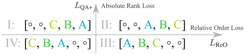
Figure 2: Relative order attack v.s. absolute rank attack.

Adversarial Ranking. In applications such as web retrieval, documents may be promoted in rankings by intentional manipulation [20]. Likewise, the existence of aforementioned works inspired attacks against deep ranking, but it is still insufficiently explored. In light of distinct purposes, ranking attacks can be divided into absolute rank attacks and relative order attacks. Most absolute rank attacks attempt to induce random “misranking” [48, 30, 33, 56, 57, 51, 58, 5, 18, 31]. Some other attacks against ranking model aim to incur purposeful changes in absolute rank, i.e., to raise or lower the ranks of specific candidates [4, 60]. On the contrary, the relative order attacks remains under-explored. And this is the first work that tampers the relative order in deep ranking.

As shown in Fig. 2, relative order is “orthogonal” to absolute rank. Let “$\circ$” denote any uninterested candidate. Suppose the selected candidates ${\mathbb{C}}$ and permutation ${\mathbf{p}}$ are [A, B, C] and $[3,2,1]$, respectively. The exemplar absolute rank loss $L_{\text{QA+}}$ [60] is ignorant to the difference in relative order comparing I and II, or IV and III. The relative order loss $L_{\text{ReO}}$ proposed in this paper is ignorant to the difference in absolute rank comparing I and IV, or II and III. Although focusing on different aspects of ranking, the two types of loss functions can be combined and jointly optimized.

3 Adversarial Order Attack

Typically, a deep ranking model is built upon deep metric learning [52, 42, 59, 26, 41]. Given a query ${\bm{q}}$ and a set of candidates ${\mathbb{C}}=\{{\bm{c}}_{1},{\bm{c}}_{2},\ldots,{\bm{c}}_{k}\}$ selected from database ${\mathbb{D}}$ (${\mathbb{C}}\subset{\mathbb{D}}$), a deep ranking model $f$ evaluates the distance between every pair of query and candidate, i.e., $f:\mathcal{I}\times\mathcal{I}\mapsto{\mathbb{R}}$ where $\mathcal{I}=[0,1]^{D}$. Thus, by comparing all the pairwise distances $\{f({\bm{q}},{\bm{c}}_{i})|i=1,2,\ldots,k\}$, the whole candidate set can be ranked with respect to the given query. For instance, the model outputs the ranking list ${\bm{c}}_{1}\prec{\bm{c}}_{2}\prec\cdots\prec{\bm{c}}_{k}$ if it determines $f({\bm{q}},{\bm{c}}_{1})<f({\bm{q}},{\bm{c}}_{2})<\cdots<f({\bm{q}},{\bm{c}}_{k})$.

Based on these, Order Attack (OA) aims to find an imperceptible perturbation ${\bm{r}}$ ($\|{\bm{r}}\|_{\infty}\leqslant\varepsilon$ and $\tilde{{\bm{q}}}={\bm{q}}+{\bm{r}}\in\mathcal{I}$), so that $\tilde{{\bm{q}}}$ as the adversarial query can convert the relative order of the selected candidates into ${\bm{c}}_{p_{1}}\prec{\bm{c}}_{p_{2}}\prec\cdots\prec{\bm{c}}_{p_{k}}$, where ${\mathbf{p}}=[p_{1},p_{2},\ldots,p_{k}]$ is a permutation vector predefined by the attacker. In particular, we assume that the attacker is inclined to select the candidate set ${\mathbb{C}}$ from the top-$N$ ranked candidates ${\mathbb{X}}$, as the ranking lists returned to the clients are usually “truncated” (i.e., only the top-ranked candidates will be shown). We call the length $N$ ($N\geqslant k$) of the “truncated” list as a “visible range”. The white-box and black-box OA will be discussed in Sec.3.1 and Sec.3.2 respectively. For sake of brevity, we let $\Omega_{\bm{q}}=\{{\bm{r}}|~{}{\bm{q}}+{\bm{r}}\in\mathcal{I},~{}\|{\bm{r}}\|_{\infty}\leqslant\varepsilon\}$.

3.1 Triplet-style Loss Function for White-Box OA

During the training process, a typical deep ranking model $f$ involves a triplet (anchor ${\bm{q}}$, positive ${\bm{c}}_{\text{p}}$, negative ${\bm{c}}_{\text{n}}$) in each iteration. In order to rank ${\bm{c}}_{\text{p}}$ ahead of ${\bm{c}}_{\text{n}}$, the model is penalized when $f({\bm{q}},{\bm{c}}_{\text{p}})+\gamma<f({\bm{q}},{\bm{c}}_{\text{n}})$ does not hold. This inequality can be reformulated exploiting the form of a hinge loss [40], resulting in the triplet ranking loss function [42] $L_{\text{triplet}}({\bm{q}},{\bm{c}}_{\text{p}},{\bm{c}}_{\text{n}})=[\gamma+f({\bm{q}},{\bm{c}}_{\text{p}})-f({\bm{q}},{\bm{c}}_{\text{n}})]^{+}$, where $[\cdot]^{+}=\max(0,\cdot)$, and $\gamma$ denotes the margin hyper-parameter.

Inspired by this, to implement the OA, we decompose the inequality chain prescribed by the predefined permutation vector ${\mathbf{p}}$, namely $f(\tilde{{\bm{q}}},{\bm{c}}_{p_{1}}){<}f(\tilde{{\bm{q}}},{\bm{c}}_{p_{2}}){<}\cdots{<}f(\tilde{{\bm{q}}},{\bm{c}}_{p_{k}})$ into $(^{k}_{2}){=}k(k{-}1)/2$ inequalities, i.e., $f(\tilde{{\bm{q}}},{\bm{c}}_{p_{i}})<f(\tilde{{\bm{q}}},{\bm{c}}_{p_{j}})$, $i,j{=}1,2,\ldots,k,~{}i{<}j$. Reformulation of these inequalities into the hinge loss form leads to the relative order loss,

$$L_{\text{ReO}}(\tilde{{\bm{q}}};{\mathbb{C}},{\mathbf{p}})=\sum_{i=1}^{k}\sum_{j=i}^{k}\big{[}f(\tilde{{\bm{q}}},{\bm{c}}_{p_{i}})-f(\tilde{{\bm{q}}},{\bm{c}}_{p_{j}})\big{]}^{+}.$$ (1)

Subsequently, given this loss function, the OA can be cast as a constrained optimization problem,

$${\bm{r}}^{\ast}=\operatorname*{arg\,min}_{{\bm{r}}\in\Omega_{\bm{q}}}L_{\text{ReO}}({\bm{q}}+{\bm{r}};{\mathbb{C}},{\mathbf{p}}),$$ (2)

which can be solved with first-order-gradient-based methods such as Projected Gradient Descent (PGD) [34], i.e.,

$${\bm{r}}_{t+1}=\text{Clip}_{\Omega_{\bm{q}}}\big{\{}{\bm{r}}_{t}-\eta\text{sign}\big{[}\nabla_{\bm{r}}L_{\text{ReO}}(\tilde{{\bm{q}}};{\mathbb{C}},{\mathbf{p}})\big{]}\big{\}},$$ (3)

where $\eta$ is the PGD step size, and ${\bm{r}}_{0}$ is initialized as a zero vector. PGD stops at a predefined maximum iteration $T$, and the final ${\bm{r}}_{T}$ is the desired adversarial perturbation.

It is worth noting that query image semantics can be drastically changed even with a very slight perturbation [60]. As a result, candidates ${\mathbb{C}}$ are prone to be excluded from the topmost part of ranking, and become invisible when the ranking result is “truncated”. To mitigate such side effect, we follow [60] and introduce a semantics-preserving term $L_{\text{QA+}}(\tilde{{\bm{q}}},{\mathbb{C}})$ to keep ${\mathbb{C}}$ within the topmost part of the ranking by raising their absolute ranks, i.e., to keep ${\bm{c}}\in{\mathbb{C}}$ ranked ahead of other candidates. Finally, the relative order loss term $L_{\text{ReO}}(\cdot)$ and the absolute rank loss term $L_{\text{QA+}}(\cdot)$ are combined to form the complete white-box OA loss $L_{\text{OA}}$,

$$L_{\text{OA}}(\tilde{{\bm{q}}};{\mathbb{C}},{\mathbf{p}})=L_{\text{ReO}}(\tilde{{\bm{q}}};{\mathbb{C}},{\mathbf{p}})+\xi L_{\text{QA+}}(\tilde{{\bm{q}}},{\mathbb{C}}),$$ (4)

where $\xi$ is a positive constant balancing factor between the relative order and absolute rank goals.

Despite the formulation of Eq. (4), an ideal $\tilde{{\bm{q}}}$ that fully satisfy the desired relative order of ${\mathbb{C}}$ does not necessarily exist. Consider a Euclidean embedding space, where candidates ${\bm{c}}_{1},{\bm{c}}_{2},{\bm{c}}_{3}$ lie consecutively on a straight line. It is impossible to find a query embedding that leads to ${\bm{c}}_{1}\prec{\bm{c}}_{3}\prec{\bm{c}}_{2}$. That indicates the compatibility between the specified relative order and the factual geometric relations of the candidate embeddings affects the performance upper-bound of OA. In cases like this, our algorithm can still find an inexact solution that satisfies as many inequalities as possible to approximate the specified relative order. In light of this, Kendall’s ranking correlation $\tau$ [24] between the specified relative order and the real ranking order appears to be a more reasonable performance metric than the success rate for OA.

3.2 Short-range Ranking Correlation

A concrete triplet-style implementation of OA is present in Sec. 3.1, but it is infeasible in a real-world attack scenario. In particular, multiple challenges are present for black-box OA, including (1) Gradient inaccessibility. The gradient of the loss w.r.t the input is inaccessible, as the network architecture and parameters are unknown; (2) Lack of similarity (or distance) scores. Exact similarity scores rarely appear in the truncated ranking results; (3) Truncated ranking results. In practice, a ranking system only presents the top-$N$ ranking results to the clients; (4) Limited query budget. Repeated, intensive queries within a short time frame may be identified as threats, e.g., Denial of Service (DoS) attack. Therefore, it is preferable to construct adversarial examples within a reasonable amount of queries. These restrictions collectively invalidate the triplet-style method.

To address these challenges, we present the “Short-range Ranking Correlation” (SRC; denoted as $\tau{S}$) metric, a practical approximation of the $L_{\text{OA}}$ (Eq. 4) as a surrogate loss function for black-box OA.

Specifically, to calculate $\tau{S}$ given ${\mathbb{C}}$, ${\mathbf{p}}$ and the top-$N$ retrieved candidates ${\mathbb{X}}$ w.r.t query $\tilde{{\bm{q}}}$, we first initialize a $(k\times k)$-shaped zero matrix ${\bm{S}}$, and permute ${\mathbb{C}}$ into ${\mathbb{C}}_{\mathbf{p}}=\{{\bm{c}}_{p_{1}},{\bm{c}}_{p_{2}},\ldots,{\bm{c}}_{p_{k}}\}$. Assuming $\forall{\bm{c}}_{i},{\bm{c}}_{j}\in{\mathbb{C}}_{\mathbf{p}}$ ($i>j,i\neq j$) exist in ${\mathbb{X}}$, we define $({\bm{c}}_{i},{\bm{c}}_{j})$ as a concordant pair as long as $\text{R}_{{\mathbb{C}}_{\mathbf{p}}}({\bm{c}}_{i})$ and $\text{R}_{{\mathbb{X}}}({\bm{c}}_{i})$ are simultaneously greater or smaller than $\text{R}_{{\mathbb{C}}_{\mathbf{p}}}({\bm{c}}_{j})$ and $\text{R}_{{\mathbb{X}}}({\bm{c}}_{j})$, respectively, where $\text{R}_{{\mathbb{X}}}({\bm{c}}_{i})$ denotes the integer rank value of ${\bm{c}}_{i}$ in ${\mathbb{X}}$, i.e., $\text{R}_{{\mathbb{X}}}({\bm{c}}_{i}):=\arg_{m}\{{\bm{c}}_{i}={\bm{x}}_{m}\}$. Otherwise, $({\bm{c}}_{i},{\bm{c}}_{j})$ is defined as a discordant pair. Namely a concordant matches a part of the specified permutation, and could result in a zero loss term in Eq. 1, while a discordant pair does not match, and could result in a positive loss term in Eq. 1. Thus, in order to approximate the relative order loss $L_{\text{ReO}}$ (Eq. 1), a concordant pair and a discordant pair will be assigned a score of $S_{i,j}=+1$ (as reward) and $S_{i,j}=-1$ (as penalty), respectively. Apart from that, when ${\bm{c}}_{i}$ or ${\bm{c}}_{j}$ does not exist in ${\mathbb{X}}$, $S_{i,j}$ will be directly assigned with an “out-of-range” penalty $-1$, which approximates the semantics-preserving term in Eq. 4. Finally, after comparing the ordinal relationships of every pair of candidates and assigning penalty values in ${\bm{S}}$, the average score of the lower triangular of ${\bm{S}}$ excluding the diagonal is the $\tau{S}$, as summarized in Algo. 1.

Input: Selected candidates ${\mathbb{C}}=\{{\bm{c}}_{1},{\bm{c}}_{2},\ldots,{\bm{c}}_{k}\}$, permutation vector ${\mathbf{p}}=[p_{1},p_{2},\ldots,p_{k}]$, top-$N$ retrieval ${\mathbb{X}}=\{{\bm{x}}_{1},{\bm{x}}_{2},\ldots,{\bm{x}}_{N}\}$ for $\tilde{{\bm{q}}}$. Note that ${\mathbb{C}}\subset{\mathbb{D}}$, ${\mathbb{X}}\subset{\mathbb{D}}$, and $N\geqslant k$.

Output: SRC coefficient $\tau{S}$.

Permute candidates as ${\mathbb{C}}_{\mathbf{p}}=\{{\bm{c}}_{p_{1}},{\bm{c}}_{p_{2}},\ldots,{\bm{c}}_{p_{k}}\}$;

Initialize score matrix ${\bm{S}}=\mathbf{0}$ of size ${k\times k}$;

for $i\leftarrow 1,2,\ldots,k$ do

      for $j\leftarrow 1,2,\ldots,i-1$ do

           if ${\bm{c}}_{i}\notin{\mathbb{X}}$   or ${\bm{c}}_{j}\notin{\mathbb{X}}$  then

                $S_{i,j}=-1$ // out-of-range

               

          else if [$\text{R}_{{\mathbb{C}}_{\mathbf{p}}}({\bm{c}}_{i}){>}\text{R}_{{\mathbb{C}}_{\mathbf{p}}}({\bm{c}}_{j})$ and $\text{R}_{{\mathbb{X}}}({\bm{c}}_{i}){>}\text{R}_{{\mathbb{X}}}({\bm{c}}_{j})$] or [$\text{R}_{{\mathbb{C}}_{\mathbf{p}}}({\bm{c}}_{i}){<}\text{R}_{{\mathbb{C}}_{\mathbf{p}}}({\bm{c}}_{j})$ and $\text{R}_{{\mathbb{X}}}({\bm{c}}_{i})<\text{R}_{{\mathbb{X}}}({\bm{c}}_{j})$]  then

                $S_{i,j}=+1$ //   concordant

               

          else if [$\text{R}_{{\mathbb{C}}_{\mathbf{p}}}({\bm{c}}_{i}){>}\text{R}_{{\mathbb{C}}_{\mathbf{p}}}({\bm{c}}_{j})$ and $\text{R}_{{\mathbb{X}}}({\bm{c}}_{i}){<}\text{R}_{{\mathbb{X}}}({\bm{c}}_{j})$] or [$\text{R}_{{\mathbb{C}}_{\mathbf{p}}}({\bm{c}}_{i}){<}\text{R}_{{\mathbb{C}}_{\mathbf{p}}}({\bm{c}}_{j})$ and $\text{R}_{{\mathbb{X}}}({\bm{c}}_{i}){>}\text{R}_{{\mathbb{X}}}({\bm{c}}_{j})$]  then

                $S_{i,j}=-1$ //   discordant

               

return $\tau{S}=\sum_{i,j}S_{i,j}/(^{k}_{2})$

Algorithm 1 Short-range Ranking Correlation $\tau{S}$.

The value of $\tau{S}$ $\in[-1,1]$ reflects the real ranking order’s alignment to the order specified by ${\mathbf{p}}$, where a semantics-preserving penalty is spontaneously incorporated. When the specified order is fully satisfied, i.e., any pair of ${\bm{c}}_{i}$ and ${\bm{c}}_{j}$ is concordant, and none of the elements in ${\mathbb{C}}$ disappear from ${\mathbb{X}}$, $\tau{S}$ will be $1$. In contrast, when every candidate pair is discordant or absent from the top-$N$ result ${\mathbb{X}}$, $\tau{S}$ will be $-1$. Overall, $(\tau{S}+1)/2$ percent of the candidate pairs are concordant, and the rest are discordant or “out-of-range”.

Maximization of $\tau{S}$ leads to the best alignment to the specified permutation, as discordant pairs will be turned into concordant pairs, while maintaining the presence of ${\mathbb{C}}$ within the top-$N$ visible range. Thus, although non-differentiable, the $\tau{S}$ metric can be used as a practical surrogate objective for black-box OA, i.e., ${\bm{r}}^{\ast}=\operatorname*{arg\,max}_{{\bm{r}}\in\Omega_{\bm{q}}}\tau{S}(\tilde{{\bm{q}}};{\mathbb{C}},{\mathbf{p}})$, which achieves a very similar effect to the white-box OA.

Particularly, when $\forall{\bm{c}}\in{\mathbb{C}}$ exists in ${\mathbb{X}}$, $\tau{S}$ degenerates into Kendall’s $\tau$ [24] between ${\mathbf{p}}$ and the permutation of ${\mathbb{C}}$ in ${\mathbb{X}}$. Namely, $\tau{S}$ also degenerates gracefully to $\tau$ in the white-box scenario because the whole ranking is visible. However, $\tau$ is inapplicable on truncated ranking results.

$\tau{S}$ does not rely on any gradient or any similarity score, and can adapt to truncated ranking results. When optimized with an efficient black-box optimizer (e.g., NES [22]), the limited query budget can also be efficiently leveraged. Since all the black-box challenges listed at the beginning of this section are handled, it is practical to perform black-box OA by optimizing $\tau{S}$ in real-world applications.

	$k=5$					$k=10$					$k=25$
$\varepsilon$	0	$\frac{2}{255}$	$\frac{4}{255}$	$\frac{8}{255}$	$\frac{16}{255}$	0	$\frac{2}{255}$	$\frac{4}{255}$	$\frac{8}{255}$	$\frac{16}{255}$	0	$\frac{2}{255}$	$\frac{4}{255}$	$\frac{8}{255}$	$\frac{16}{255}$
Fashion-MNIST   $N=\infty$
$\tau{S}$	0.000	0.286	0.412	0.548	0.599	0.000	0.184	0.282	0.362	0.399	0.000	0.063	0.108	0.136	0.149
mR	2.0	4.5	9.1	12.7	13.4	4.5	7.4	10.9	15.2	17.4	12.0	16.1	17.6	18.9	19.4
Stanford Online Products   $N=\infty$
$\tau{S}$	0.000	0.396	0.448	0.476	0.481	0.000	0.263	0.348	0.387	0.398	0.000	0.125	0.169	0.193	0.200
mR	2.0	5.6	4.9	4.2	4.1	4.5	12.4	11.2	9.9	9.6	12.0	31.2	28.2	25.5	25.4

Table 1: White-box order attack on Fashion-MNIST and SOP datasets with various settings.

$\xi$	$0$	$10^{-1}$	$10^{0}$	$10^{1}$	$10^{2}$	$10^{3}$	$10^{4}$	$10^{5}$	$10^{6}$	$10^{7}$
Fashion-MNIST   $k=5$, $N=\infty$, $\varepsilon=4/255$
$\tau{S}$	0.561	0.467	0.451	0.412	0.274	0.052	0.043	0.012	0.007	0.002
mR	27.2	22.7	18.3	9.1	4.9	3.2	2.8	2.7	2.7	2.7
Stanford Online Products   $k=5$, $N=\infty$, $\varepsilon=4/255$
$\tau{S}$	0.932	0.658	0.640	0.634	0.596	0.448	0.165	0.092	0.013	0.001
mR	973.9	89.8	48.1	22.4	7.5	4.9	2.9	2.8	2.8	2.7

Table 2: Searching for balancing factor $\xi$ on both datasets.

4 Experiments

To evaluate the white-box and black-box OA, we conduct experiments on the Fashion-MNIST [54] and the Stanford-Online-Products (SOP) [37] datasets which comprise images of retail commodity. Firstly, we train a CNN with $2$-convolution-$1$-fully-connected network on Fashion-MNIST, and a ResNet-18 [21] without the last fully-connected layer on SOP following [60] that focuses on the absolute rank attack. Then we perform OA with the corresponding test set as the candidate database ${\mathbb{D}}$. Additionally, we also qualitatively evaluate black-box OA on “JD SnapShop” [23] to further illustrate its efficacy. In our experiments, the value of rank function $\text{R}_{\mathbb{X}}(\cdot)$ starts from $0$, i.e., the $k$-th ranked candidate has the rank value of $k-1$.

Selection of ${\mathbb{C}}$ and ${\mathbf{p}}$. As discussed, we assume that the attacker is inclined to select the candidate set ${\mathbb{C}}$ from the top-$N$ ranked candidates given the visible range limit. For simplicity, we only investigate the $(k,N)$-OA, i.e., OA with the top-$k$-within-top-$N$ ($k\leq N$) candidates selected as as ${\mathbb{C}}$. It is representative because an OA problem with some candidates randomly selected from the top-$k$ results as ${\mathbb{C}}$ is a sub-problem of $(k,N)$-OA. Namely, our attack will be effective for any selection of ${\mathbb{C}}$ as long as the $(k,N)$-OA is effective. For white-box OA, we conduct experiments with $N{=}\infty$, and $k{\in}\{5,10,25\}$. For black-box attack, we conduct experiments with $N{=}\{\infty,50,k\}$, and $k{=}\{5,10,25\}$. A random permutation vector ${\mathbf{p}}$ is specified for each query.

Evaluation Metric. Since $\tau{S}$ is equivalent to $\tau$ when $N=\infty$, we use $\tau{S}$ as the performance metric for both white-box and black-box OA. Specifically, in each experiment, we conduct $\mathsfit{T}=10^{4}$ times of OA attack. In each attack, we randomly draw a sample from ${\mathbb{D}}$ as the query ${\bm{q}}$. In the end, we report the average $\tau{S}$ over the $\mathsfit{T}$ trials. Also, when $N=\infty$, we additionally calculate the mean rank of the candidate set ${\mathbb{C}}$ (demoted as “mR”, which equals $[\sum^{k}_{i}\text{R}_{{\mathbb{X}}}({\bm{c}}_{i})]/k$), and report the average mean rank over the $\mathsfit{T}$ attacks. Larger $\tau{S}$ value and smaller mR value are preferable.

Parameter Settings. We set the perturbation budget as $\varepsilon\in\{\frac{2}{255},\frac{4}{255},\frac{8}{255},\frac{16}{255}\}$ following [28] for both white-box and black-box attacks. The query budget $Q$ is set to $1.0\times 10^{3}$. For white-box OA, the PGD step size $\eta$ is set to $\frac{1}{255}$, the PGD step number to $24$. The balancing parameter $\xi$ is set as $10^{1}$ and $10^{3}$ for Fashion-MNIST and SOP respectively. The learning rates of black-box optimizer NES [22] and SPSA [50] are both set to $2/255$. See supplementary for more details of the black-box optimizers.

Search Space Dimension Reduction. As a widely adopted trick, dimension reduction of the adversarial perturbation search space has been reported effective in [14, 9, 44, 29]. Likewise, we empirically reduce the space to $(3\times 32\times 32)$ for black-box OA on Stanford-Online-Products dataset and “JD SnapShop”. In fact, a significant performance drop in $\tau{S}$ can be observed without this trick.

4.1 White-Box Order Attack Experiments

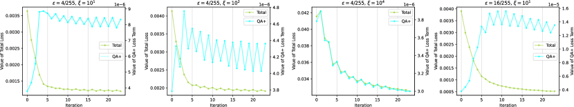
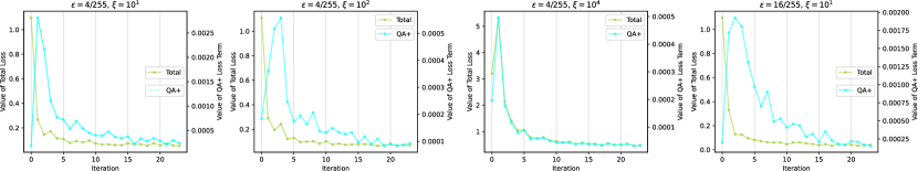
Figure 3: Curves of total loss $L_{\text{OA}}$ (left y-axis) and the $L_{\text{QA+}}$ term (right y-axis) during the optimization procedures under different $\varepsilon$ and $\xi$ settings. The first row is for Fashion-MNIST, while the second row is for SOP dataset.

The first batch of the experiments is carried out on the Fashion-MNIST dataset, as shown in the upper part of Tab. 1. With the original query image ($\varepsilon=0$), the expected $\tau{S}$ performance of $(5,\infty)$-OA is $0.000$, and the ${\mathbb{C}}$ retains their original ranks as the mR equals $2.0$. With a $\varepsilon=2/255$ adversarial perturbation budget, our OA achieves $\tau{S}=0.286$, which means on average $64.3\%$ of the inequalities reflecting the specified permutations are satisfied by the adversarial examples. Meanwhile, the mR changes from $2.0$ to $4.5$, due to adversarial perturbation can move the query embedding off its original position [60] while seeking for a higher $\tau{S}$. Nevertheless, the mR value of $4.5$ indicates that the ${\mathbb{C}}$ are still kept visible in the topmost part of the ranking result by the loss term $L_{\text{QA+}}(\cdot)$. With larger perturbation budget $\varepsilon$, the $\tau{S}$ metric increases accordingly, e.g., $\tau{S}$ reaches $0.599$ when $\varepsilon=16/255$, which means nearly $80\%$ of the inequalities are satisfied. Likewise, the experimental results on SOP are available in the lower part of Tab. 1, which also demonstrate the effectiveness of our method under different settings.

Besides, we note that different balancing parameter $\xi$ for $L_{\text{QA+}}(\cdot)$ leads to distinct results, as shown in Tab. 2. We conduct $(5,\infty)$-OA with $\varepsilon=4/255$ with different $\xi$ values ranging from $0$ to $10^{7}$ on both datasets. Evidently, a larger $\xi$ leads to a better (smaller) mR value, but meanwhile a worse $\tau{S}$ as the weighted $L_{\text{QA+}}(\cdot)$ term dominates the total loss. There is a trade-off between the $\tau{S}$ and mR, which is effectively controlled by the tunable constant parameter $\xi$. Hence, we empirically set $\xi$ as $10^{1}$ and $10^{3}$ for Fashion-MNIST and SOP respectively, in order to keep the mR of most experiments in Tab. 1 below a sensible value, i.e., $50/2$.

Additionally, Tab. 1 reveals that the mR trends w.r.t. $\varepsilon$ on the two datasets differ. To investigate this counter-intuitive phenomenon, we plot loss curves in Fig. 3. In the $\varepsilon=4/255$, $\xi=10$ case for Fashion-MNIST, the total loss decreases but the $L_{\text{QA+}}$ surges at the beginning and then plateaus. After increasing $\xi$ to $10^{2}$, the $L_{\text{QA+}}$ rises more smoothly. The curve eventually decreases at $\xi=10^{4}$, along with a small mR and a notable penalty on $\tau{S}$ as a result. Besides, the “sawtooth-shaped” $L_{\text{QA+}}$ curves also indicate that the $L_{\text{ReO}}$ term is optimized while sacrificing the mR as a side-effect at the even steps, while the optimizer turns to optimize $L_{\text{QA+}}$ at the odd steps due to the semantics-preserving penalty, causing a slight increase in $L_{\text{ReO}}$. These figures indicate that optimizing $L_{\text{ReO}}$ without sacrificing $L_{\text{QA+}}$ is difficult. Moreover, perturbation budget is irrelevant. Comparing the first and the fourth sub-figures, we find a larger budget ($\varepsilon{=}\frac{16}{255}$) unhelpful in reducing optimization difficulty as the $L_{\text{QA+}}$ curve still soars and plateaus. Based on these cues, we speculate that the different curve patterns of mR stem from the optimization difficulty due to a fixed PGD step size that cannot be smaller, and different dataset properties.

The intra-class variance of the simple Fashion-MNIST dataset is smaller than that of SOP, which means sample embeddings of the same class are densely clustered. As each update can change the ${\mathbb{X}}$ drastically, it is difficult to adjust the query embedding position in a dense area with a fixed PGD step for a higher $\tau{S}$ without significantly disorganizing the ranking list (hence a lower mR). In contrast, a larger intra-class variance of the SOP dataset makes $L_{\text{QA+}}$ easier to be maintained, as shown in the 2nd row of Fig. 3.

Algorithm	$k=5$				$k=10$				$k=25$
	$\varepsilon=\frac{2}{255}$	$\varepsilon=\frac{4}{255}$	$\varepsilon=\frac{8}{255}$	$\varepsilon=\frac{16}{255}$	$\varepsilon=\frac{2}{255}$	$\varepsilon=\frac{4}{255}$	$\varepsilon=\frac{8}{255}$	$\varepsilon=\frac{16}{255}$	$\varepsilon=\frac{2}{255}$	$\varepsilon=\frac{4}{255}$	$\varepsilon=\frac{8}{255}$	$\varepsilon=\frac{16}{255}$
None	0.0, 2.0	0.0, 2.0	0.0, 2.0	0.0, 2.0	0.0, 4.5	0.0, 4.5	0.0, 4.5	0.0, 4.5	0.0, 12.0	0.0, 12.0	0.0, 12.0	0.0, 12.0
Fasion-MNIST   $N=\infty$
Rand	0.211, 2.1	0.309, 2.3	0.425, 3.0	0.508, 7.7	0.172, 4.6	0.242, 5.0	0.322, 6.4	0.392, 12.7	0.084, 12.3	0.123, 13.1	0.173, 15.8	0.218, 25.8
Beta	0.241, 2.1	0.360, 2.6	0.478, 4.6	0.580, 19.3	0.210, 4.8	0.323, 5.7	0.430, 9.6	0.510, 30.3	0.102, 12.4	0.163, 13.8	0.237, 19.7	0.291, 42.7
PSO	0.265, 2.1	0.381, 2.3	0.477, 4.4	0.580, 21.1	0.239, 4.8	0.337, 5.7	0.424, 9.7	0.484, 34.0	0.131, 12.7	0.190, 14.6	0.248, 21.7	0.286, 54.2
NES	0.297, 2.3	0.416, 3.1	0.520, 8.7	0.630, 46.3	0.261, 5.0	0.377, 6.6	0.473, 14.3	0.518, 55.6	0.142, 13.0	0.217, 15.9	0.286, 28.3	0.312, 74.3
SPSA	0.300, 2.3	0.407, 3.2	0.465, 7.1	0.492, 16.3	0.249, 5.0	0.400, 6.6	0.507, 12.8	0.558, 27.5	0.135, 12.9	0.236, 16.3	0.319, 27.1	0.363, 46.4
Fashion-MNIST   $N=50$
Rand	0.207	0.316	0.424	0.501	0.167	0.242	0.321	0.378	0.083	0.123	0.165	0.172
Beta	0.240	0.359	0.470	0.564	0.204	0.323	0.429	0.487	0.103	0.160	0.216	0.211
PSO	0.266	0.377	0.484	0.557	0.239	0.332	0.420	0.458	0.134	0.183	0.220	0.203
NES	0.297	0.426	0.515	0.584	0.262	0.378	0.463	0.458	0.141	0.199	0.223	0.185
SPSA	0.292	0.407	0.468	0.490	0.253	0.397	0.499	0.537	0.131	0.214	0.260	0.275
Fashion-MNIST   $N=k$
Rand	0.204	0.289	0.346	0.302	0.146	0.181	0.186	0.124	0.053	0.062	0.049	0.021
Beta	0.237	0.342	0.372	0.275	0.183	0.236	0.218	0.106	0.072	0.079	0.058	0.020
PSO	0.252	0.342	0.388	0.284	0.198	0.240	0.219	0.081	0.080	0.082	0.046	0.013
NES	0.274	0.360	0.381	0.282	0.198	0.234	0.213	0.113	0.071	0.076	0.055	0.016
SPSA	0.274	0.360	0.412	0.427	0.188	0.251	0.287	0.298	0.067	0.086	0.091	0.095

Table 3: Black-box OA on Fashion-MNIST dataset. In the $N=\infty$ experiments, ($\tau{S}$, mR) are reported in each cell, while only $\tau{S}$ is reported in the cells when $N$ equals $50$ or $k$. A larger $k$ and a smaller $N$ make the attack harder.

4.2 Black-Box Order Attack Experiments

To simulate a real-world attack scenario, we convert the ranking models trained for Sec. 4.1 into black-box versions, which are subject to limitations discussed in Sec. 3.2. Black-box OA experiments are conducted on these models.

To optimize the surrogate loss $\tau{S}$, we adopt and compare several black-box optimizers: (1) Random Search (Rand), which independently samples every dimension of ${\bm{r}}$ from uniform distribution $\mathcal{U}(-\varepsilon,+\varepsilon)$, then clips it to $\Omega_{\bm{q}}$; (2) Beta-Attack (Beta), a modification of $\mathcal{N}$-Attack [32] that generates the ${\bm{r}}$ from an iteratively-updated Beta distribution (instead of Gaussian) per dimension; (3) Particle Swarm Optimization (PSO) [43], a classic meta-heuristic black-box optimizer with an extra step that clips the adversarial perturbation to $\Omega_{\bm{q}}$; (4) NES [22, 53], which performs PGD [34] using estimated gradient; (5) SPSA [50, 46], which can be interpreted as NES using a different sampling distribution.

Dataset	$k$	Rand	Beta	PSO	NES	SPSA	SRC Time
Fashion-MNIST	5	0.195	0.386	0.208	0.208	0.202	0.080
Fashion-MNIST	10	0.206	0.404	0.223	0.214	0.213	0.087
Fashion-MNIST	25	0.228	0.435	0.249	0.236	0.235	0.108
SOP	5	1.903	2.638	1.949	1.882	1.783	0.091
SOP	10	1.923	2.720	1.961	1.954	1.836	0.095
SOP	25	1.936	2.745	1.985	1.975	1.873	0.117

Table 4: Run time (second) per $(k,50)$-OA adversarial example for different black-box methods. $\varepsilon{=}\frac{4}{255}$ and $Q{=}10^{3}$.

We first investigate the black-box $(5,\infty)$-OA, as shown in the upper part ($N{=}\infty$) of Tab. 3 and Tab. 5. In these cases, $\tau{S}$ does not pose any semantics-preserving penalty since $N{=}\infty$, which is similar to white-box attack with $\xi{=}0$. With the Rand optimizer, $\tau{S}$ can be optimized to $0.309$ with $\varepsilon{=}\frac{4}{255}$ on Fashion-MNIST. As $\varepsilon$ increases, we obtain better $\tau{S}$ results, and larger mR values as an expected side-effect.

Algorithm	$k=5$				$k=10$				$k=25$
	$\varepsilon=\frac{2}{255}$	$\varepsilon=\frac{4}{255}$	$\varepsilon=\frac{8}{255}$	$\varepsilon=\frac{16}{255}$	$\varepsilon=\frac{2}{255}$	$\varepsilon=\frac{4}{255}$	$\varepsilon=\frac{8}{255}$	$\varepsilon=\frac{16}{255}$	$\varepsilon=\frac{2}{255}$	$\varepsilon=\frac{4}{255}$	$\varepsilon=\frac{8}{255}$	$\varepsilon=\frac{16}{255}$
None	0.0, 2.0	0.0, 2.0	0.0, 2.0	0.0, 2.0	0.0, 4.5	0.0, 4.5	0.0, 4.5	0.0, 4.5	0.0, 12.0	0.0, 12.0	0.0, 12.0	0.0, 12.0
Stanford Online Product   $N=\infty$
Rand	0.187, 2.6	0.229, 8.5	0.253, 85.8	0.291, 649.7	0.167, 5.6	0.197, 13.2	0.208, 92.6	0.222, 716.4	0.093, 14.1	0.110, 27.6	0.125, 146.7	0.134, 903.7
Beta	0.192, 3.3	0.239, 15.3	0.265, 176.7	0.300, 1257.7	0.158, 6.2	0.186, 19.9	0.207, 139.0	0.219, 992.5	0.099, 15.5	0.119, 37.1	0.119, 206.5	0.132, 1208.5
PSO	0.122, 2.1	0.170, 3.0	0.208, 13.3	0.259, 121.4	0.135, 4.8	0.177, 6.5	0.206, 22.8	0.222, 166.5	0.104, 12.7	0.122, 16.7	0.137, 49.5	0.140, 264.2
NES	0.254, 3.4	0.283, 15.6	0.325, 163.0	0.368, 1278.7	0.312, 7.2	0.351, 26.3	0.339, 227.1	0.332, 1486.7	0.242, 18.0	0.259, 51.5	0.250, 324.1	0.225, 1790.8
SPSA	0.237, 3.5	0.284, 11.9	0.293, 75.2	0.318, 245.1	0.241, 7.8	0.325, 22.2	0.362, 112.7	0.383, 389.0	0.155, 18.1	0.229, 41.9	0.286, 185.6	0.306, 557.8
Stanford Online Product   $N=50$
Rand	0.180	0.216	0.190	0.126	0.163	0.166	0.119	0.055	0.092	0.055	0.016	0.003
Beta	0.181	0.233	0.204	0.119	0.153	0.168	0.116	0.054	0.084	0.057	0.021	0.003
PSO	0.122	0.173	0.183	0.153	0.135	0.164	0.137	0.081	0.093	0.083	0.042	0.011
NES	0.247	0.283	0.246	0.152	0.314	0.295	0.195	0.077	0.211	0.136	0.054	0.013
SPSA	0.241	0.287	0.297	0.303	0.233	0.298	0.298	0.292	0.125	0.130	0.114	0.103
Stanford Online Product   $N=k$
Rand	0.148	0.100	0.087	0.026	0.094	0.044	0.018	0.001	0.023	0.009	0.002	0.001
Beta	0.136	0.106	0.053	0.025	0.076	0.040	0.010	0.004	0.021	0.004	0.001	0.001
PSO	0.102	0.098	0.059	0.031	0.088	0.049	0.022	0.007	0.040	0.015	0.006	0.001
NES	0.185	0.139	0.076	0.030	0.173	0.097	0.036	0.008	0.071	0.027	0.007	0.005
SPSA	0.172	0.154	0.141	0.144	0.107	0.104	0.085	0.069	0.026	0.025	0.017	0.016

Table 5: Black-box OA on Stanford Online Product dataset. In the $N=\infty$ experiments, ($\tau{S}$, mR) are reported in each cell, while only $\tau{S}$ is reported in the cells when $N$ equals $50$ or $k$. A larger $k$ and a smaller $N$ make the attack harder.

Since all the queries of Rand are independent, one intuitive way towards better performance is to leverage the historical query results and adjust the search distribution. Following this, we modify $\mathcal{N}$-Attack [32] into Beta-Attack, replacing its Gaussian distributions into Beta distributions, from which each element of ${\bm{r}}$ is independently generated. All the Beta distribution parameters are initialized as $1$, where Beta degenerates into Uniform distribution (Rand). During optimization, the probability density functions are modified according to $\tau{S}$ results, in order to increase the expectation of the next adversarial perturbation drawn from these distributions. Results in Tab. 3 suggest Beta’s advantage against Rand, but it also shows that the Beta distributions are insufficient for modeling the perturbation ${\bm{r}}$ for OA.

According to the $(k,\infty)$-OA results in Tab. 3 and Tab. 5, NES and SPSA outperform Rand, Beta and PSO. This means black-box optimizers based on estimated gradient are still the most effective and efficient for $(k,\infty)$-OA. A larger $\varepsilon$ leads to a unanimous increase in $\tau{S}$ metric, and a side effect of worse (larger) mR. Predictably, when $N{=}50$ or $k$, the algorithms may confront a great penalty due to the absence of the selected candidates from the top-$N$ visible range.

Further results of $(k,50)$-OA and $(k,k)$-OA confirm our speculation, as shown in the middle ($N{=}50$) and bottom ($N{=}k$) parts of Tab. 3 and Tab. 5. With $N{=}50$ and a fixed $\varepsilon$, algorithms that result in a small mR (especially for those with $\text{mR}{<}\frac{50}{2}$) also perform comparably as in $(k,\infty)$-OA. Conversely, algorithms that lead to a large mR in $(k,\infty)$-OA are greatly penalized in $(k,50)$-OA. The results also manifest a special characteristic of OA, that $\tau{S}$ peaks at a certain small $\varepsilon$, and does not positively correlate with $\varepsilon$. This is rather apparent in difficult settings such as $(k,k)$-OA on SOP dataset. In brief, the optimizers based on estimated gradients still perform the best in $(k,50)$-OA and $(k,k)$-OA, and an excessively large perturbation budget is not necessary.

All these experiments demonstrate the effectiveness of optimizing the surrogate objective $\tau{S}$ to conduct black-box OA. As far as we know, optimizers based on gradient estimation are the most reliable choices. Next, we adopt SPSA and perform practical OA in real-world applications.

Algorithm	$\varepsilon$	$k$	$Q$	$\mathsfit{T}$	Mean $\tau{S}$	Stdev $\tau{S}$	Max $\tau{S}$	Min $\tau{S}$	Median $\tau{S}$
SPSA	1/255	5	100	204	0.390	0.373	1.000	-0.600	0.400
SPSA	1/255	10	100	200	0.187	0.245	0.822	-0.511	0.200
SPSA	1/255	25	100	153	0.039	0.137	0.346	-0.346	0.033

Table 6: Quantitative $(k,50)$-OA Results on JD Snapshop.

Time Complexity. Although the complexity of Algo. 1 is $\mathcal{O}(k^{2})$, the actual run time of our Rust-based SRC implementation is short, as measured with Python cProfile with a Xeon 5118 CPU and a GTX1080Ti GPU. As shown in Tab. 4, SRC calculation merely consumes $0.117$ seconds on average across the five algorithms for an adversarial example on SOP with $k=25$. The overall time consumption is dominated by sorting and PyTorch [38] model inference. Predictably, in real-world attack scenarios, It is highly likely that the time consumption bottleneck stems from other factors irrelevant to our method, such as network delays and bandwidth, or the query-per-second limit set by the service provider.

4.3 Practical Black-Box Order Attack Experiments

“JD SnapShop” [23] is an e-commerce platform based on content-based image retrieval [45]. Clients can upload query merchandise images via an HTTP-protocol-based API, and then obtain the top-$50$ similar products. This exactly matches the setting of $(k,50)$-OA. As the API specifies a file size limit ($\leqslant$ 3.75MB), and a minimum image resolution ($128{\times}128$), we use the standard $(224{\times}224)$ size for the query. We merely provide limited evaluations because the API poses a hard limit of $500$ queries per day per user.

As noted in Sec. 4.2, the $\tau{S}$ peaks with a certain small $\varepsilon$. Likewise, an empirical search for $\varepsilon$ suggests that $1/255$ and $2/255$ are the most suitable choices for OA against “JD SnapShop”. Any larger $\varepsilon$ value easily leads to the disappearance of ${\mathbb{C}}$ from ${\mathbb{X}}$. This is meanwhile a preferable characteristic, as smaller perturbations are less perceptible.

As shown in Fig. 1, we select the top-$5$ candidates as ${\mathbb{C}}$, and specify ${\mathbf{p}}{=}[1,5,4,3,2]$. Namely, the expected relative order among ${\mathbb{C}}$ is ${\bm{c}}_{1}{\prec}{\bm{c}}_{5}{\prec}{\bm{c}}_{4}{\prec}{\bm{c}}_{3}{\prec}{\bm{c}}_{2}$. By maximizing the $\tau{S}$ with SPSA and $\varepsilon{=}\frac{1}{255}$, we successfully convert the relative order to the specified one using $200$ times of queries. This shows that performing OA by optimizing our proposed surrogate loss $\tau{S}$ with a black-box optimizer is practical. Some limited quantitative results are presented in Tab. 6, where $Q$ is further limited to $100$ in order to gather more data, while a random permutation and a random query image from SOP is used for each of the $\mathsfit{T}$ times of attacks.

Algorithm	$\varepsilon$	$k$	$Q$	$\mathsfit{T}$	Mean $\tau{S}$	Stdev $\tau{S}$	Max $\tau{S}$	Min $\tau{S}$	Median $\tau{S}$
SPSA	$8/255$	5	100	105	0.452	0.379	1.000	-0.400	0.600
SPSA	$8/255$	10	100	95	0.152	0.217	0.733	-0.378	0.156
SPSA	$8/255$	25	100	93	0.001	0.141	0.360	-0.406	0.010

Table 7: $(k,50)$-OA Results on Bing Visual Search API.

We also conduct OA against Bing Visual Search API [35] following the same protocol. We find this API less sensitive to weak (i.e., $\varepsilon{=}\frac{1}{255}$) perturbations unlike Snapshop, possibly due to a different data pre-processing pipeline. As shown in Tab. 7, our OA is also effective against this API.

In practice, the adversarial example may be slightly changed by transformations such as the lossy JPEG/PNG compression, and resizing (as a pre-processing step), which eventually leads to changes on the $\tau{S}$ surface. But a black-box optimizer should be robust to such influences.

5 Conclusion

Deep ranking systems inherited the adversarial vulnerabilities of deep neural networks. In this paper, the Order Attack is proposed to tamper the relative order among selected candidates. Multiple experimental evaluations of the white-box and black-box Order Attack illustrate their effectiveness, as well as the deep ranking systems’ vulnerability in practice. Ranking robustness and fairness with respect to Order Attack may be the next valuable direction to explore. Code: https://github.com/cdluminate/advorder.

Acknowledgement. This work was supported partly by National Key R&D Program of China Grant 2018AAA0101400, NSFC Grants 62088102, 61976171, and XXXXXXXX, and Young Elite Scientists Sponsorship Program by CAST Grant 2018QNRC001.

Appendix A Order Attack against “JD SnapShop” API

A.1 More Technical Details

We present additional technical details about the “JD SnapShop” API [23] and the Fig. 1:

1. Since the perturbation tensor contains negative values, it is normalized before being displayed in Fig. 1:

   $$\text{Normalize}({\bm{r}})=0.5+0.5*{\bm{r}}/\max\big{(}\text{abs}({\bm{r}})\big{)}.$$ (5)

2. Since the selected candidates ${\mathbb{C}}$ are [A, B, C, D, E], and the permutation vector is ${\mathbf{p}}=[1,5,4,3,2]$, the expected relative order among ${\mathbb{C}}$ is ${\mathbb{C}}_{p_{1}}\prec{\mathbb{C}}_{p_{2}}\prec{\mathbb{C}}_{p_{3}}\prec{\mathbb{C}}_{p_{4}}\prec{\mathbb{C}}_{p_{5}}$, i.e., A $\prec$ E $\prec$ D $\prec$ C $\prec$ B.

3. Each product corresponds to multiple images. Only the default product images specified by the service provider are displayed in the figure.

4. The API in fact provides a similarity score for every candidate, which indeed can be leveraged for, e.g., better gradient estimation. However, the other practical ranking applications may not necessarily provide these similarity scores. Hence, we simply ignore such discriminative information to deliberately increase the difficulty of attack. The concrete ways to take advantage of known similarity scores are left for future works.

5. In Fig. 1, the original similarity scores of candidates from A to E are [ $0.7132$, $0.6336$, $0.6079$, $0.5726$, $0.5700$]. With our adversarial query, the scores of A to E are changed into [ $0.6960$, $0.5724$, $0.5763$, $0.5827$, $0.5898$].

6. The API supports a “topK” argument, which enables the clients to change the visible range $N$. We leave it as the recommended default value $50$.

7. From Fig. 1, we note some visually duplicated images among the candidates. For instance, there are many other candidates similar to candidate E, due to reasons such as different sellers reusing the same product image. These images are not adjacent to each other in the ranking list, since the platform assigns them with different similarity scores. For instance, the $5$-th and $8$-th candidates in the first row of Fig. 1 are assigned with similarity scores $[0.5700,0.5521]$, while the $2$-nd, $7$-th, and $10$-th items in the second row are assigned with similarity scores $[0.5898,0.5728,0.5536]$. Whether the calculation of similarity scores involves multiple cues (e.g., by aggregating the similarity scores of multiple product images, or using information from other modalities such as text), or even engineering tricks are unknown and beyond the scope of discussion.

8. Users (with the free plan) are merely allowed to perform $500$ times of queries per day as a hard limit.

9. The API documentation can be found at
   https://aidoc.jd.com/image/snapshop.html.

10. The SKU ID atop every candidate image can be used to browse the real product webpages on the “JingDong” shopping platform. The URL format is
    https://item.jd.com/<SKU-ID>.html
    For example, the webpage for the product with SKU ID 72210617020 is located at
    https://item.jd.com/72210617020.html
    Note, due to irresistible reasons such as sellers withdrawing their product webpage and the ranking algorithm/database updates, some of the links may become invalid during the review process, and the ranking result for the same query may change.

11. It consumes 200 times of queries to find the adversarial example presented in Fig. 1. This process takes around 170 seconds, mainly due our limited network condition.

A.2 Empirical Search for $\varepsilon$ on the API

According to the white-box and black-box OA experiments in the manuscript, we learn that the perturbation budget $\varepsilon$ affects the OA performance. And it meanwhile controls the adversarial perturbation imperceptibility. Thus, we search for a proper $\varepsilon$ for OA against “JD SnapShop”. Due to the limitation that only $500$ times of queries per day are allowed for each user, we merely present some empirical and qualitative observation for different $\varepsilon$ settings.

As shown in Tab. 8, we test the “JD SnapShop” API with adversarial query images using the Rand algorithm with different $\varepsilon$ values. We conduct $50$ times of attack per value. Our qualitative observation is summarized in the table.

$\varepsilon$	Empirical Qualitative Observation
$16/255$	Almost any $\forall{\bm{c}}\in{\mathbb{C}}$ disappear from the top-$N$ candidates, resulting in $\tau{S}\approx-1$.
$8/255$	In most cases only $0\sim 1$ selected candidate remains within the top-$N$ result.
$4/255$	In most cases only $1\sim 3$ selected candidates remain within the top-$N$ result.
$2/255$	Nearly all ${\bm{c}}\in{\mathbb{C}}$ remain in top-$N$ with significant order change. (suitable for ${\mathbf{p}}$ with $p_{1}\neq 1$)
$1/255$	Top-$1$ seldom moves. The rest part is slightly changed. (suitable for ${\mathbf{p}}$ with $p_{1}=1$)

Table 8: Empirical & Qualitative Parameter Search for $\varepsilon$ on “JD SnapShop”.

From the table, we find that $\varepsilon=1/255$ and $\varepsilon=2/255$ are the most suitable choices for the $(5,50)$-OA against “JD SnapShop”. This is meanwhile very preferable since such slight perturbations are imperceptible to human. As shown in Fig. 4, the $\varepsilon=1/255,2/255,4/255$ adversarial perturbation can hardly be perceived, but the largest perturbation (i.e., $\varepsilon=16/255$) used by [28] is relatively visible.

$\varepsilon=0$

$\varepsilon=1/255$

$\varepsilon=2/255$

$\varepsilon=4/255$

$\varepsilon=8/255$

$\varepsilon=16/255$

Figure 4: Imperceptibility: Images perturbed under different perturbation budgets. A large perturbation with $\varepsilon=16/255$ is already relatively visible. However, in fact, $\varepsilon=1/255$ and $\varepsilon=2/255$ are more suitable choices for OA against “JD SnapShop”, because they are least visible, and may lead to the best $\tau{S}$.

A.3 More Showcases of OA against the API

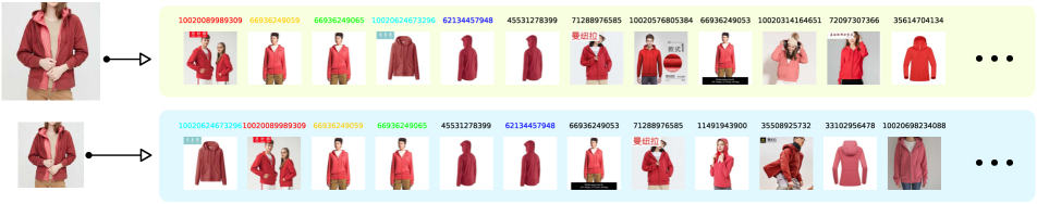
Figure 8: Showcase #2: “Red wind coat” query image with $\varepsilon=2/255$ perturbation.

• In showcase #2 (Fig.8), the original similarity scores of the top-$5$ candidates are [ $0.7551$, $0.6586$, $0.6586$, $0.6533$, $6507$]. They are changed into [ $0.6748$, $0.6723$, $0.6723$, $0.6921$, $0.6609$] with the perturbation.

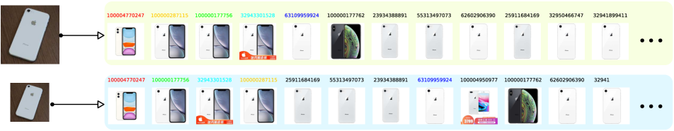
Figure 9: Showcase #3: “iPhone” query image with $\varepsilon=1/255$ perturbation.

• In showcase #3 (Fig.9), the original top-$5$ candidate similarity [ $0.8522$, $0.8333$, $0.8341$, $0.7659$, $0.7159$] is changed into [ $0.8792$, $0.7928$, $0.8470$, $0.7958$, $0.7130$].

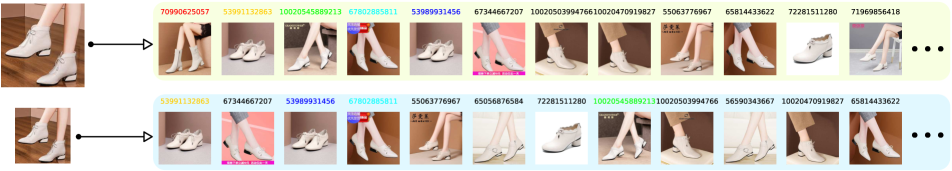
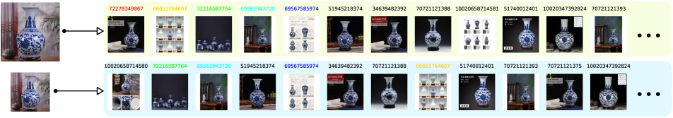
Figure 10: Two cases (“Shoe” and “Vase”) where the top-$1$ ranked candidate disappear from the top-ranked results.

• Fig. 10 shows two examples where one selected candidate disappear from top-$N$ result with our adversarial query. In the “white shoes” case, the top-$5$ candidate similarity scores are changed from [ $0.8659$, $0.8653$, $0.8648$, $0.8619$, $0.8603$] to [ N/A, $0.8689$, $0.8603$, $0.8640$, $0.8641$]. In the “vase” case, the top-$5$ candidate similarity scores are changed from [ $0.9416$, $0.9370$, $0.9360$, $0.9350$, $0.9349$] to [ N/A, $0.9338$, $0.9427$, $0.9392$, $0.9361$].

• Fig. 11 shows some long-tail queries on which our OA will not take effect, because a large portion of the top-ranked candidates have completely the same similarity scores. In the 1st row, i.e., results for a “Machine Learning” textbook query, the similarity scores of the $5$-th to $7$-th candidates are $0.9242$. The score of the $9$-th to $11$-th candidates are $0.9240$. That of the $22$-th to $50$-th are the same $0.9202525$. In the “Deep Learning” textbook case (2nd row), the similarity scores of the $27$-th to $50$-th candidates are $0.9288423$. In the “RTX 3090 GPU” case (3rd row), the similarity scores of the $7$-th to $9$-th candidate are unexceptionally $0.5581$. OA cannot change the relative order among those candidates with the same similarity scores.

Appendix B Visualizing Black-Box OA on Fashion-MNIST & Stanford Online Products

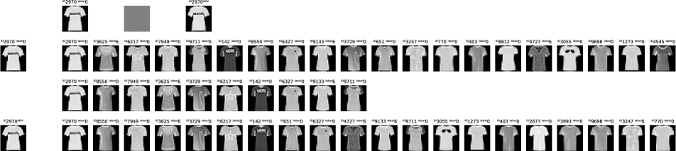
Figure 14: Fashion-MNIST Showcase #3. $k=10$, $\tau{S}=1.0$

We present some visualizations of the black-box OA on the Fashion-MNIST dataset and the SOP dataset, as shown in (Fig. 14, Fig. 14, Fig. 14) and (Fig. 17, Fig. 17, Fig. 17), respectively. All the adversarial perturbations are found under $\varepsilon=4/255$ and $N=50$.

All these figures are picture matrices of size $(4,2+2k)$. In particular, pictures at location $(1,3)$, $(1,5)$ and $(1,7)$ are the original query, the perturbation and the perturbed query image, respectively. The 2nd row in each figure is the original query and the corresponding ranking list (truncated to the top-$2k$ results). The 3rd row in each figure is the permuted top-$k$ candidates. The 4th row in each figure is the adversarial query and the corresponding ranking list (also truncated to the top-$2k$ results). Every picture is annotated with its ID in the dataset and its label for classification.

Appendix C Additional Information for White-Box OA

C.1 Example case where an ideal $\tilde{q}$ is impossible

As discussed in Sec. 3.1, an ideal adversarial example that fully satisfy the desired relative order does not always exist. As an example, let ${\bm{v}}_{q},{\bm{v}}_{1},{\bm{v}}_{2},{\bm{v}}_{3}$ be the embeddings of $\tilde{{\bm{q}}},{\bm{c}}_{1},{\bm{c}}_{2},{\bm{c}}_{3}$ mentioned in the last paragraph of Sec. 3.1, respectively. Assume the embeddings are non-zero vectors, ${\bm{v}}_{1}{=}{\bm{v}}_{2}{-}{\bm{o}}$, ${\bm{v}}_{3}{=}{\bm{v}}_{2}{+}{\bm{o}}$, where vector ${\bm{o}}{\neq}0$. Then a specified permutation ${\bm{c}}_{1}{\prec}{\bm{c}}_{3}{\prec}{\bm{c}}_{2}$, namely $f(\tilde{{\bm{q}}},{\bm{c}}_{1}){<}f(\tilde{{\bm{q}}},{\bm{c}}_{3}){<}f(\tilde{{\bm{q}}},{\bm{c}}_{2})$ requires $-({\bm{v}}_{q}^{T}{\bm{o}}-{\bm{v}}_{2}^{T}{\bm{o}})>{\bm{v}}_{q}^{T}{\bm{o}}-{\bm{v}}_{2}^{T}{\bm{o}}$ and ${\bm{v}}_{q}^{T}{\bm{o}}-{\bm{v}}_{2}^{T}{\bm{o}}>0$, which are contradictory to each other. Thus, there is no satisfactory ${\bm{v}}_{q}$.

C.2 More Results on Ablation of $L_{\text{QA+}}$

	$k=5$					$k=10$					$k=25$
$\varepsilon$	0	$\frac{2}{255}$	$\frac{4}{255}$	$\frac{8}{255}$	$\frac{16}{255}$	0	$\frac{2}{255}$	$\frac{4}{255}$	$\frac{8}{255}$	$\frac{16}{255}$	0	$\frac{2}{255}$	$\frac{4}{255}$	$\frac{8}{255}$	$\frac{16}{255}$
Fashion-MNIST   $\xi=0$
$\tau{S}$	0.000	0.336	0.561	0.777	0.892	0.000	0.203	0.325	0.438	0.507	0.000	0.077	0.131	0.170	0.189
mR	2.0	5.5	27.2	52.7	75.6	4.5	8.0	17.3	40.4	63.4	12.0	16.4	19.2	22.8	25.3
Stanford Online Products   $\xi=0$
$\tau{S}$	0.000	0.932	0.970	0.975	0.975	0.000	0.632	0.760	0.823	0.832	0.000	0.455	0.581	0.646	0.659
mR	2.0	973.9	1780.1	2325.5	2421.9	4.5	1222.7	3510.2	5518.6	6021.4	12.0	960.4	2199.2	3321.4	3446.3

Table 9: More Results of White-Box OA with $\xi=0$ (i.e., without the $L_{\text{QA+}}$ term). These results are supplementary to Tab. 2 in the manuscript.

In order to make sure the selected candidates ${\mathbb{C}}$ will not disappear from the top-$N$ results during the OA process, a semantics-preserving term $L_{\text{QA+}}$ is introduced to maintain the absolute ranks of ${\mathbb{C}}$. Tab. 2 in the manuscript presents two ablation experimental results of $L_{\text{QA+}}$ for the white-box $(5,\infty)$-OA with $\varepsilon=4/255$. In this subsection, we provide the full ablation experiments of $L_{\text{QA+}}$ in all parameter settings, as shown in Tab. 9. After removing the $L_{\text{QA+}}$ term from the loss function (i.e., setting $\xi=0$), the white-box OA can achieve a better $\tau{S}$, meanwhile a worse mR. When comparing it with Tab. 1 in the manuscript, we find that (1) the semantics-preserving term $L_{\text{QA+}}$ is effective for keeping the selected $C$ within top-$N$ results; (2) $L_{\text{QA+}}$ will increase the optimization difficulty, so there will be a trade off between $L_{\text{ReO}}$ and $L_{\text{QA+}}$. These results support our analysis and discussion in Sec. 4.1.

C.3 Transferability

Some adversarial examples targeted at ranking models have been found transferable [60]. Following [60], we train Lenet and ResNet18 models on Fashion-MNIST besides the C2F1 model used in the manuscript. Each of them is trained with two different parameter initializations (annotated with #1 and #2). Then we conduct transferability-based attack using a white-box surrogate model with $k=5$ and $\varepsilon=\frac{4}{255}$, as shown in Tab. 10.

From \ To	Lenet #1	Lenet #2	C2F1 #1	C2F1 #2	ResNet18 #1	ResNet18 #2
Lenet #1	0.377	-0.003	0.013	-0.014	0.003	0.010
C2F1 #1	0.016	0.003	0.412	0.005	0.020	0.008
ResNet18 #1	-0.001	-0.011	-0.006	0.020	0.268	0.016

Table 10: OA Example Transferability Experiment.

According to the table, OA adversarial example does not exhibit transferability over different architectures or different parameter initializations. We believe these models learned distinct embedding spaces, across which enforcing a specific fixed ordering is particularly difficult without prior knowledge of the model being attacked. As transferability is not a key point of the manuscript, we only discuss it in this appendix.

C.4 Intra-Class Variance & OA Difficulty

In the last paragraph of Sec. 4.1 (White-Box Order Attack Experiments), it is claimed that,

The intra-class variance of the relatively simple Fashion-MNIST dataset is smaller than that of SOP, which means samples of the same class are densely clustered in the embedding space. As each update could change the ${\mathbb{X}}$ more drastically, it is more difficult to adjust the query embedding position with a fixed PGD step for a higher $\tau{S}$ without sacrificing the mR value.

To better illustrate the idea, a diagram is present in Fig. 5. Given a trained model, and a fixed PGD step size as $1/255$, the query image is projected near a dense embedding cluster in case I, while near a less dense embedding cluster in case II. Then the query image is updated with a fixed step size in both case I and case II, resulting in similar position change in the embedding space. At the same time the ranking list for the updated query will change as well. However, the ranking list in case I changes much more dramatically than that in case II. As a result, there is a higher chance for the ranks of the selected ${\mathbb{C}}$ to significantly change in case I, leading to a high value of mR. Besides, $1/255$ is already the smallest appropriate choice for the PGD update step size, as in practice the adversarial examples will be quantized into the range $[0,255]$. Namely, the position of the query embedding cannot be modified in a finer granularity given such limitation. Since a dataset with small intra-class variance tend to be densely clustered in the embedding space, we speculate that optimizing $L_{\text{OA}}$ on a dataset with small intra-class variance (e.g., Fashion-MNIST) is difficult, especially in terms of maintaining a low mR.

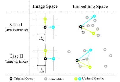
Figure 5: Intra-Class Variance & OA Difficulty. Updated queries are linked to two closest candidates with doted lines.

Algorithm	$N=\infty$    $k=5$				$N=50$    $k=5$				$N=5$    $k=5$
	$\varepsilon=\frac{2}{255}$	$\frac{4}{255}$	$\frac{8}{255}$	$\frac{16}{255}$	$\frac{2}{255}$	$\frac{4}{255}$	$\frac{8}{255}$	$\frac{16}{255}$	$\frac{2}{255}$	$\frac{4}{255}$	$\frac{8}{255}$	$\frac{16}{255}$
None	0.0, 2.0	0.0, 2.0	0.0, 2.0	0.0, 2.0	0.0	0.0	0.0	0.0	0.0	0.0	0.0	0.0
Rand (w/o DR)	0.106, 2.1	0.151, 3.1	0.190, 13.1	0.224, 117.5	0.101	0.139	0.167	0.148	0.076	0.086	0.058	0.026
Rand (w/ DR)	0.187, 2.6	0.229, 8.5	0.253, 85.8	0.291, 649.7	0.180	0.216	0.190	0.126	0.148	0.100	0.087	0.026
Beta (w/o DR)	0.120, 2.2	0.158, 3.8	0.199, 21.8	0.231, 205.7	0.115	0.164	0.173	0.141	0.097	0.096	0.060	0.035
Beta (w/ DR)	0.192, 3.3	0.239, 15.3	0.265, 176.7	0.300, 1257.7	0.181	0.233	0.204	0.119	0.136	0.106	0.053	0.025
PSO (w/o DR)	0.128, 2.1	0.174, 3.1	0.219, 13.0	0.259, 122.0	0.133	0.175	0.199	0.155	0.097	0.095	0.060	0.036
PSO (w/ DR)	0.122, 2.1	0.170, 3.0	0.208, 13.3	0.259, 121.4	0.122	0.173	0.183	0.153	0.102	0.098	0.059	0.031
NES (w/o DR)	0.139, 2.3	0.192, 4.8	0.244, 31.9	0.266, 300.0	0.128	0.192	0.208	0.166	0.108	0.102	0.079	0.039
NES (w/ DR)	0.254, 3.4	0.283, 15.6	0.325, 163.0	0.368, 1278.7	0.247	0.283	0.246	0.152	0.185	0.139	0.076	0.030
SPSA (w/o DR)	0.135, 2.4	0.171, 3.9	0.209, 15.9	0.226, 45.2	0.140	0.176	0.205	0.223	0.108	0.110	0.146	0.143
SPSA (w/ DR)	0.237, 3.5	0.284, 11.9	0.293, 75.2	0.318, 245.1	0.241	0.287	0.297	0.303	0.172	0.154	0.141	0.144

Table 11: Ablation study of the search space Dimension Reduction (DR) trick for black-box OA with SOP dataset.

Appendix D Additional Information for Black-Box OA

D.1 Average query number for successful attack

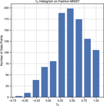
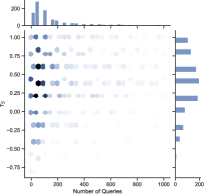
Figure 6: Histogram of $\tau{S}$ (left) and hexbin plot with marginal histogram for $\tau{S}$ and its respective query number (right) of $(5,50)$-OA on Fashion-MNIST.

As shown in Fig. 6, we plot the histogram (left) of $\tau{S}$ for $1000$ trials of $(5,50)$-OA with SPSA ($\varepsilon=4/255$, $Q=10^{3}$) on Fashion-MNIST, as well as a hexbin plot with marginal histogram for $\tau{S}$ and its respective query number (right), where $106$ trials reach $\tau{S}=1.0$ with $226.4$ queries on average.

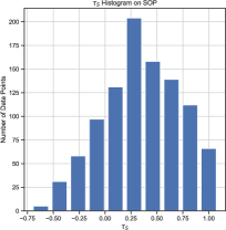
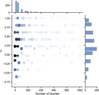
Figure 7: Histogram of $\tau{S}$ (left) and hexbin plot with marginal histogram for $\tau{S}$ and its respective query number (right) of $(5,50)$-OA on SOP.

Following the same setting, the plots with $1000$ trials of $(5,50)$-OA on SOP is also available in Fig. 7, where $66$ trials reach $\tau{S}=1.0$ with $213.6$ queries on average.

D.2 Relation between Query Budget $Q$ and $\tau{S}$

Predictably, the query budget $Q$ could significantly impact the $\tau{S}$ as it directly limits the max number of iterations for any given black-box optimizer. To study such impact, we conduct experiments on the Fashion-MNIST dataset, as shown in Tab. 12. It is clear that the performance of all black-box optimizers become better with the query budget $Q$ increasing, but will eventually plateau. Even with an extremely limited query budget $Q=10^{2}$, the methods based on estimated gradients remain to be the most effective ones.

Algorithm	Fashion-MNIST   $N=\infty$, $k=5$, $\varepsilon=\frac{4}{255}$
	$Q=10^{2}$	$5\times 10^{2}$	*$10^{3}$	$5\times 10^{3}$	$10^{4}$
Rand	0.233, 2.2	0.291, 2.2	0.309, 2.3	0.318, 2.2	0.320, 2.2
Beta	0.249, 2.2	0.313, 2.4	0.360, 2.6	0.368, 2.6	0.382, 2.4
PSO	0.280, 2.6	0.341, 2.4	0.381, 2.3	0.382, 2.4	0.385, 2.4
NES	0.309, 2.6	0.380, 2.9	0.416, 3.1	0.431, 2.9	0.438, 2.9
SPSA	0.292, 2.6	0.365, 2.8	0.407, 3.2	0.421, 2.9	0.433, 2.8

Table 12: $\tau{S}$ with different query budget $Q$.

D.3 Ablation of Search Space Dimension Reduction

In this subsection, we study the effectiveness of the dimension reduction trick, which has been widely adopted in the literature [14, 9, 44, 29]. As shown in Tab. 11, all black-box optimizers benefit from this trick except for PSO, as illustrated by the performance gains. We leave the analysis on the special characteristics of PSO for future work.

D.4 Random Initialization

Some black-box classification attacks such as [6] initializes the adversarial perturbation as a random vector. However, we note that the adversarial perturbation for OA should be always initialized as a zero vector, because random initialization is harmful.

For white-box OA, a random initial perturbation may dramatically change the query semantics and push the query embedding off its original position by a large margin [60]. Thus, the expectation of the initial mR will be higher, hence an avoidable query semantics-preserving penalty will be triggered. Then, the optimizer will have to “pull” the adversarial query back near its original location in the embedding space, during which it may even stuck at a local optimum.

For black-box OA, the random initialization could be harmful for the methods based on estimated gradient, such as NES and SPSA, because the adversarial query may directly lie on a “flat” area of the $\tau{S}$ surface, where all the selected candidates disappear from the top-$N$ and all the neighboring samples lead to $\tau{S}=-1$ as well. The estimated gradient will be invalid, hence OA will fail. In contrast, zero vector initialization could largely mitigate such difficulties.

Appendix E Defense Against OA

According to [60] which presents a defense method for deep ranking, our proposed OA also requires the query embedding to be moved to a proper position. Thus, the defense [60] that reduces the embedding move distance is expected to be resistant to our OA to some extent. To validate this, we conduct white-box attack on a defensed model as shown in Tab. 13, as well as black-box attack (with SPSA) on a defensed model as shown in Tab. 14.

$\varepsilon$	Fashion-MNIST ($N=\infty$)						Stanford Online Product ($N=\infty$)
	$k=5$		$k=10$		$k=25$		$k=5$		$k=10$		$k=25$
	$\tau{S}$	mR	$\tau{S}$	mR	$\tau{S}$	mR	$\tau{S}$	mR	$\tau{S}$	mR	$\tau{S}$	mR
2/255	0.098	2.0	0.069	4.6	0.033	12.1	0.216	2.1	0.190	4.7	0.093	12.4
4/255	0.176	2.1	0.122	4.7	0.059	12.3	0.306	2.4	0.294	5.1	0.148	13.0
8/255	0.271	2.4	0.207	4.9	0.096	12.6	0.381	2.6	0.380	5.9	0.206	13.8
16/255	0.384	3.1	0.304	5.8	0.137	13.4	0.526	3.2	0.433	6.8	0.249	14.7

Table 13: White-Box attack against a defensed model [60].

$\varepsilon$	Fashion-MNIST						Stanford Online Product
	$N=\infty$			$N=50$			$N=\infty$			$N=50$
	$k=5$	$k=10$	$k=25$	$k{=}5$	$k{=}10$	$k{=}25$	$k=5$	$k=10$	$k=25$	$k{=}5$	$k{=}10$	$k{=}25$
2/255	0.114, 2.0	0.099, 4.6	0.052, 12.1	0.113	0.099	0.050	0.057, 2.0	0.058, 4.5	0.041, 12.0	0.058	0.061	0.042
4/255	0.154, 2.1	0.156, 4.7	0.090, 12.2	0.156	0.158	0.089	0.075, 2.0	0.109, 4.6	0.086, 12.1	0.075	0.102	0.082
8/255	0.172, 2.2	0.217, 4.9	0.138, 12.8	0.178	0.216	0.131	0.082, 2.0	0.133, 4.7	0.128, 12.4	0.073	0.138	0.131
16/255	0.177, 2.3	0.259, 5.4	0.167, 13.8	0.179	0.259	0.165	0.068, 2.1	0.162, 4.9	0.158, 13.2	0.069	0.159	0.162

Table 14: Black-Box attack against a defensed model [60].

According to the tables, the defense is moderately effective against OA. Further analysis is left for future work.

Appendix F Difference from Absolute Rank Attack

The equations in Sec. 3.1 are similar to those in [60] to make the method self-contained. Although visually similar to QA+ [60], $L_{\text{ReO}}$ in Eq. 1 has a different goal:
Besides, we also contribute a surrogate objective (Short-range Ranking Correlation) in Sec. 3.2 for black-box OA.

Appendix G Application & Influence of OA

On popular online shopping platforms, sales of a product closely correlates to the click-through rate (CTR). Furthermore, the ranking position has significant impacts on its CTR, per sponsored search advertising literature [10, 39]. Specifically, “the observed CTR is geometrically decreasing as the position lowers down, exhibiting a good fit to the gamma signature.” [10]. In practice, $\text{Gamma}(1.2,0.01)$ distribution is used to model this position effect, whose value is highly sensitive to even subtle changes in ranking positions. Take the Taobao.com (mobile version) as an example, only 4 slots are typically shown in each page of retrieval with the first being paid promotion. For advertisers, the cost difference between the 1st page Ads and 2nd page Ads is dramatic, which indicates the monetary value of this attack (e.g., moving a good’s position from 4th to 3th leads to its appearance on the 1st page of retrieval results).

To help the reader better understand the motivation and potential influence of OA, we elaborate on a concrete example about how it may be used in practice.

Recall a claim in the Introduction of the manuscript: “Such vulnerability in a commercial platform may be exploited in a malfeasant business competition among the top-ranked products, e.g., via promoting fraudulent web pages containing adversarial example product images.” Assume product A is the best seller of its kind. Product B and C are A’s alternatives and business competitors, but are less prevalent. When a client searches with product image of A, product A, B, and C will be ranked near the topmost part of the list and presented to the client, while A is ranked ahead of B and C. Then, an attacker may want to to increase B’s and C’s sales leveraging A’s popularity and advertising effects. Product C may have a higher priority than B because the producer of C invested more money to the attacker.

An attacker may first setup a third-party product promotion website displaying images of product A, but these images are actually adversarially perturbed with Order Attack to make B and C ranked ahead of A, and C ahead of B without introducing obviously wrong retrieval results. Namely, this website is pretending to promote product A, but is actually promoting product C and B as their relative order has been changed into C $\prec$ B $\prec$ A. When a user clicks an adversarially perturbed product image of A, the image is used as a query, and the user will first see product C, then B, finally A. Such subtle changes in relative order can be sufficient to impact the relative sales of product A, B and C. Thus, this is an example of “malfeasant business competition” which cannot be achieved by pure absolute rank attacks. Ways to guide users to such websites, e.g., phishing or hijacking user requests, are beyond the scope of discussion.

Figure 11: Three long-tail query cases (Two “Textbooks” and “Graphics Card”) where OA will not be effective as expected.

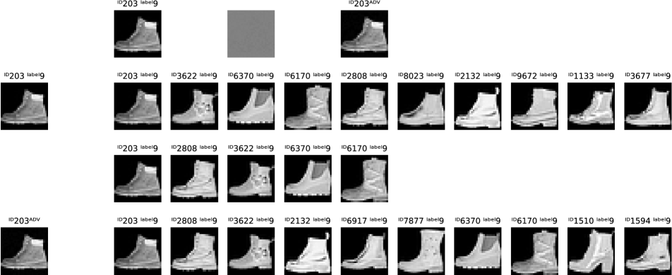
Figure 12: Fashion-MNIST Showcase #1. $k=5$, $\tau{S}=1.0$

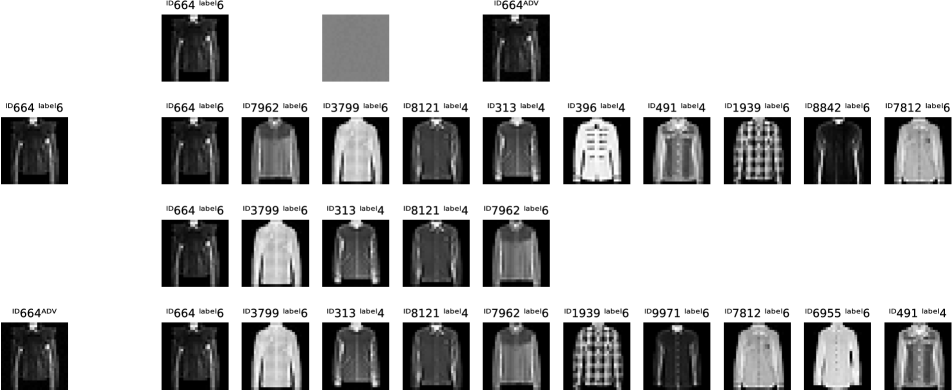
Figure 13: Fashion-MNIST Showcase #2. $k=5$, $\tau{S}=1.0$

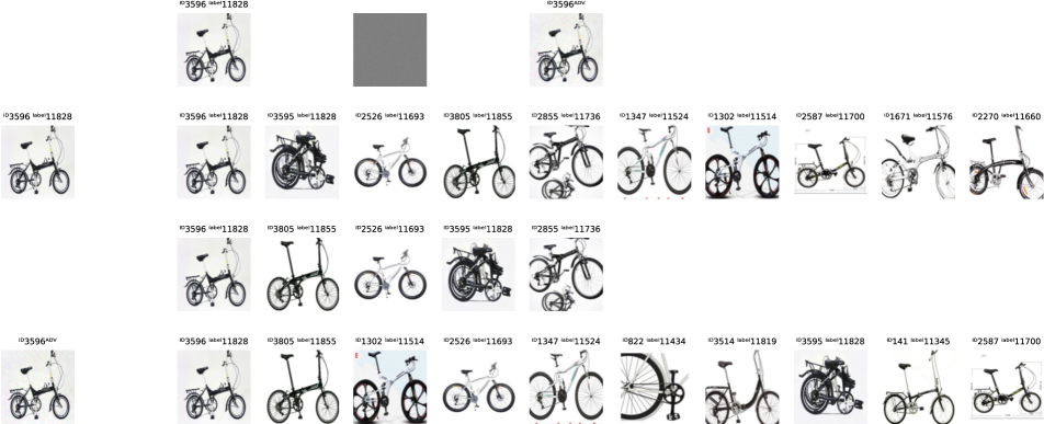
Figure 15: SOP Showcase #1. $k=5$, $\tau{S}=1.0$

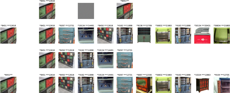
Figure 16: SOP Showcase #2. $k=5$, $\tau{S}=1.0$

Figure 17: SOP Showcase #3. $k=10$, $\tau{S}=0.96$

Appendix H Black-Box Optimizer Details

In this section, we present the black-box optimization algorithm details for (1) Random Search (Rand); (2) Beta-Attack (Beta); (3) Particle Swarm Optimization (PSO) [43]; (4) Natural Evolution Strategy (NES) [22, 53]; and (5) Simultaneous Perturbation Stochastic Approximation (SPSA) [50, 46]. Experimental results of parameter search for every optimization algorithm are also provided.

H.1 Random Search (Rand)

As a baseline algorithm for black-box optimization, Random Search assumes each element in the adversarial perturbation to be i.i.d, and samples each element from the uniform distribution within $\Omega_{\bm{q}}$, namely ${\bm{r}}=[r_{1},r_{2},\ldots,r_{D}]$ where $r_{i}\sim\mathcal{U}(-\varepsilon,+\varepsilon)$ ($i=1,2,\ldots,D$) in each iteration. The output of the algorithm is the best historical result, as summarized in Algo.2. This algorithm is free of hyper-parameters.

This algorithm will never be stuck at a local-maxima, which means it has a great ability to search for solutions from the global scope. But its drawback is meanwhile clear, as each trial of this algorithm is independent to each other. In our implementation, we conduct OA on a batch of random perturbations to accelerate the experiments, with the batch size set as $H=50$.

Input: Query Image ${\bm{q}}$, Query Budget $Q$, Selected Candidates ${\mathbb{C}}$, Permutation vector ${\mathbf{p}}$

Output: Adversarial Query $\tilde{{\bm{q}}}$

Initialize $\tilde{{\bm{q}}}\leftarrow{\bm{q}}$, and the best score $s^{\ast}\leftarrow\tau{S}(\tilde{{\bm{q}}})$;

for $i\leftarrow 1,2,\ldots,Q$ do

       Sample ${\bm{r}}\sim\mathcal{U}^{D}(-\varepsilon,+\varepsilon)$;

       if $\tau{S}\Big{(}\text{Clip}_{\Omega_{\bm{q}}}({\bm{q}}+{\bm{r}})\Big{)}>s^{\ast}$ then

             $\tilde{{\bm{q}}}\leftarrow\text{Clip}_{\Omega_{\bm{q}}}({\bm{q}}+{\bm{r}})$ ;

            $s^{\ast}\leftarrow\tau{S}\Big{(}\text{Clip}_{\Omega_{\bm{q}}}({\bm{q}}+{\bm{r}})\Big{)}$ ;

return $\tilde{{\bm{q}}}$

Algorithm 2 Rand: Naïve Random Search.

H.2 Beta-Attack (Beta)

Beta-Attack is modified from $\mathcal{N}$-Attack [32]. Although similar, a notable difference between them is that the Gaussian distributions in $\mathcal{N}$-Attack are replaced with Beta distributions. We choose Beta distribution because the shape of its probability density function is much more flexible than that of the Gaussian distribution, which may be beneficial for modeling the adversarial perturbations. Besides, according to our observation, $\mathcal{N}$-Attack is too prone to be stuck at a local maxima for OA, leading to a considerably low $\tau{S}$.

The key idea of Beta-Attack is to find the parameters for a parametric distribution $\pi({\bm{z}}|\bm{\theta})$ from which the adversarial perturbations drawn from it is likely adversarially effective. For Beta-Attack, $\pi({\bm{z}}|\bm{\theta})$ is a combination of $D$ independent Beta distributions , with parameter $\bm{\theta}=[{\bm{a}};{\bm{b}}]$ where ${\bm{a}}=[a_{1},a_{2},\ldots,a_{D}]$, ${\bm{b}}=[b_{1},b_{2},\ldots,b_{D}]$, and $z_{i}\sim\text{Beta}(a_{i},b_{i})\in[0,1],~{}(i=1,2,\ldots,D)$. Let $\mathcal{T}({\bm{z}})=\tau{S}\big{(}\text{Clip}_{\Omega_{\bm{q}}}({\bm{q}}+\varepsilon(2{\bm{z}}-1))\big{)}$, where $\varepsilon(2{\bm{z}}-1)={\bm{r}}$ is the adversarial perturbation. We hope to maximize the mathematical expectation of $\mathcal{T}({\bm{z}})$ over distribution $\pi({\bm{z}}|\bm{\theta})$:

$$\max_{\mathbf{\theta}}\mathbb{E}_{\pi({\bm{z}}|\bm{\theta})}\Big{[}\mathcal{T}({\bm{z}})\Big{]}:=\int\mathcal{T}({\bm{z}})\cdot\pi({\bm{z}}|\bm{\theta})d{\bm{z}}$$ (6)

The gradient of the expectation with respect to $\bm{\theta}$ is

$$\nabla_{\bm{\theta}}\mathbb{E}_{\pi({\bm{z}}|\bm{\theta})}\Big{[}\mathcal{T}({\bm{z}})\Big{]}$$ (7)

$$= \nabla_{\bm{\theta}}\int\mathcal{T}({\bm{z}})\cdot\pi({\bm{z}}|\bm{\theta})d{\bm{z}}$$ (8)

$$= \int\mathcal{T}({\bm{z}})\cdot\frac{\pi({\bm{z}}|\bm{\theta})}{\pi({\bm{z}}|\bm{\theta})}\nabla_{\bm{\theta}}\pi({\bm{z}}|\bm{\theta})d{\bm{z}}$$ (9)

$$= \int\pi({\bm{z}}|\bm{\theta})\cdot\mathcal{T}({\bm{z}})\cdot\nabla_{\bm{\theta}}\log\big{[}\pi({\bm{z}}|\bm{\theta})\big{]}d{\bm{z}}$$ (10)

$$= \mathbb{E}_{\pi({\bm{z}}|\bm{\theta})}\Big{[}\mathcal{T}({\bm{z}})\cdot\nabla_{\bm{\theta}}\log\big{[}\pi({\bm{z}}|\bm{\theta})\big{]}\Big{]}$$ (11)

where

$$\nabla_{\bm{\theta}}\log\big{[}\pi({\bm{z}}|\bm{\theta})\big{]} =\Big{[}\nabla_{\bm{a}}\log\big{[}\pi({\bm{z}}|\bm{\theta})\big{]};~{}\nabla_{\bm{b}}\log\big{[}\pi({\bm{z}}|\bm{\theta})\big{]}\Big{]},$$ (12)

$$\nabla_{\bm{a}}\log\big{[}\pi({\bm{z}}|\bm{\theta})\big{]} =\psi^{(0)}({\bm{a}}+{\bm{b}})-\psi^{(0)}({\bm{a}})+\log({\bm{z}}),$$ (13)

$$\nabla_{\bm{b}}\log\big{[}\pi({\bm{z}}|\bm{\theta})\big{]} =\psi^{(0)}({\bm{a}}+{\bm{b}})-\psi^{(0)}({\bm{b}})+\log(1-{\bm{z}}),$$ (14)

and $\psi^{(n)}(z)$ is the $n$-th derivative of the digamma function. The Eq. 8 to Eq. 14 means that the gradient of the expectation of $\mathcal{T}({\bm{z}})$ with respect to $\theta$ can be estimated by approximating the expectation in Eq. 11 with its mean value using a batch of random vectors, i.e.,

$$\mathbb{E}_{\pi({\bm{z}}|\bm{\theta})}\Big{[}\mathcal{T}({\bm{z}})\cdot\nabla_{\bm{\theta}}\log\big{[}\pi({\bm{z}}|\bm{\theta})\big{]}\Big{]}$$ (15)

$$\approx \frac{1}{H}\sum_{i=1}^{H}\Big{[}\mathcal{T}({\bm{z}}_{i})\cdot\nabla_{\bm{\theta}}\log\big{[}\pi({\bm{z}}_{i}|\bm{\theta})\big{]}\Big{]}$$ (16)

where $H$ denotes the batch size, and ${\bm{z}}_{i}$ is drawn from $\pi({\bm{z}}|\bm{\theta})$. Thus, the parameters $\bm{\theta}$ of the Beta distributions can be updated with Stochastic Gradient Ascent, i.e.,

$${\bm{\theta}}_{t+1}\leftarrow\bm{\theta}_{t}+\eta\nabla_{\bm{\theta}}\mathbb{E}_{\pi({\bm{z}}|\mathbf{\bm{\theta}})}\Big{[}\mathcal{T}({\bm{z}})\Big{]},$$ (17)

where $\eta$ is a constant learning rate for the parameters $\bm{\theta}$. With a set of trained parameters $\bm{\theta}$, we expect a higher $\tau{S}$ performance from a random perturbation ${\bm{z}}$ drawn from $\pi({\bm{z}}|\bm{\theta})$.

In our experiments, we initialize ${\bm{a}}{=}1$, and ${\bm{b}}{=}1$. This is due to a important property of Beta distribution that it degenerates into Uniform distribution when $a{=}1$ and $b{=}1$. Namely, our Beta-Attack is initialized as the “Rand Search” method, but it is able to update its parameters according to the historical $\tau{S}$ results, changing the shape of its probability density function in order to improve the expectation of the $\tau{S}$ of the next adversarial perturbation drawn from it. The batch size $H$ is set to $50$ for all the experiments.

As discussed in Sec. 4.2, and shown in Tab. 3 and Tab. 5, the Beta-Attack obviously outperforms the “Rand Search”, and is comparable to PSO, but is still surpassed by NES and SPSA. Such simple parametric distributions are far not enough for modeling the adversarial perturbations for the challenging OA problem. Due to its performance not outperforming PSO, NES and SPSA, the new Beta-Attack is not regarded as a contribution of our paper, but its comparison with the other methods are still very instructive.

H.2.1 Parameter Search for Beta-Attack

Learning Rate $\eta$	0.0	1.5	*3.0	4.5	6.0
SRC $\tau{S}$	0.290, 2.2	0.332, 2.4	0.360, 2.6	0.341, 2.5	0.330, 2.5

Table 15: Parameter search of learning rate $\eta$ for Beta-Attack. Fashion-MNIST dataset, $N=\infty$, $k=5$, $\varepsilon=\frac{4}{255}$.

We conduct parameter search of $\eta$ on the Fashion-MNIST, as shown in Tab. 15. From the table, we find that the $\tau{S}$ performance peaks at $\eta=3.0$, so we set this value as the default learning rate for the experiments on Fashion-MNIST. Apart from that, we empirically set $\eta=0.5$ for the experiments on SOP following a similar parameter search.

H.3 Particle Swarm Optimization (PSO)

Particle Swarm Optimization [25, 43] is a classical meta-heuristic optimization method. Let constant $H$ denote the population (swarm) size, we randomly initialize the $H$ particles (vectors) as ${\mathbb{Y}}=\{{\bm{y}}_{1},{\bm{y}}_{2},\ldots,{\bm{y}}_{H}\}$. The positions of these particles are iteratively updated according to the following velocity formula:

$${\bm{v}}_{i}\leftarrow\omega{\bm{v}}_{i}+\text{rand()}\cdot\phi_{p}({\bm{p}}_{i}-{\bm{y}}_{i})+\text{rand()}\cdot\phi_{g}({\bm{g}}-{\bm{y}}_{i})\\$$ (18)

$${\bm{y}}_{i}\leftarrow{\bm{y}}_{i}+{\bm{v}}_{i}$$ (19)

where ${\bm{y}}_{i}\in{\mathbb{Y}}$, rand() generates a random number within the interval $[0,1]$, $\omega$ denotes the inertia (momentum), ${\bm{p}}_{i}$ is the historical best position of particle $i$, ${\bm{g}}$ is the global historical best position among all particles, $\phi_{p}$ and $\phi_{g}$ are two constant parameters. As a meta-heuristic method, PSO does not guarantee that a satisfactory solution will eventually be discovered.

In the implementation, we directly represent the adversarial query $\tilde{{\bm{q}}}$ withe the particles ${\mathbb{Y}}$. And we also additionally clip the particles at the end of each PSO iteration, i.e.,

$${\bm{y}}_{i}\leftarrow\min\Big{\{}{\bm{q}}+\varepsilon,\max\big{\{}{\bm{q}}-\varepsilon,{\bm{y}}_{i}\big{\}}\Big{\}},$$ (20)

which is the only difference of our implementation compared to the standard PSO [43]. In all our experiments, the swarm size is empirically set as $H=40$.

H.3.1 Parameter Search for PSO

Inertia $\omega$	0.8	1.0	*1.1	1.2	1.4
SRC $\tau{S}$	0.321, 2.3	0.363, 2.3	0.381, 2.3	0.369, 2.4	0.349, 2.4

Table 16: Inertia $\omega$ parameter search for PSO. Fashion-MNIST dataset, $N=\infty$, $k=5$, $\varepsilon=\frac{4}{255}$.

$\phi_{p}$	0.37	0.47	*0.57	0.67	0.77
SRC $\tau{S}$	0.353, 2.3	0.375, 2.3	0.381, 2.3	0.376, 2.3	0.364, 2.3

Table 17: $\phi_{p}$ parameter search for PSO. Fashion-MNIST dataset, $N=\infty$, $k=5$, $\varepsilon=\frac{4}{255}$.

$\phi_{g}$	0.24	0.34	*0.44	0.54	0.64
SRC $\tau{S}$	0.353, 2.3	0.372, 2.3	0.381, 2.3	0.380, 2.3	0.359, 2.3

Table 18: $\phi_{g}$ parameter search for PSO. Fashion-MNIST dataset, $N=\infty$, $k=5$, $\varepsilon=\frac{4}{255}$.

We conduct parameter search of $\omega$, $\phi_{p}$ and $\phi_{g}$ for PSO on the Fashion-MNIST dataset, as shown in Tab. 16, Tab. 17 and Tab. 18.

• Inertia $\omega$: This parameter affects the convergence of the algorithm. A large $\omega$ endows PSO with better global searching ability, while a small $\omega$ allows PSO to search better in local areas. From the table, we find the PSO performance peaks at $\omega=1.1$. The performance curve of $\tau{S}$ with respect to different $\omega$ settings suggests that the global searching ability is relatively important for solving the black-box Order Attack problem.

• Constants $\phi_{p}$ and $\phi_{g}$: These parameter control the weights of a particle’s historical best position (“the particle’s own knowledge”) and the swarm’s historical global best position (“the knowledge shared among the swarm”) in the velocity formula. With a relatively small $\phi_{p}$, and a relatively large $\phi_{g}$, the swarm will converge faster towards the global best position, taking a higher risk of being stuck at a local optimum. From the tables of parameter search, we note that both constants should be kept relatively small, which means it is not preferred to converge too fast towards either the particles’ individual best positions or the global best position, for sake of better global searching ability of the algorithm.

We conclude from the parameter search that the global searching ability is important for solving the black-box OA problem, as reflected by the parameter search. Hence, we empirically set $\omega=1.1$, $\phi_{p}=0.57$, and $\phi_{g}=0.44$ for PSO in all experiments.

H.4 Natural Evolutionary Strategy (NES)

NES [22] is based on [53], which aims to find the adversarial perturbation through projected gradient method [34] with estimated gradients. Specifically, let the adversarial query $\tilde{{\bm{q}}}$ be the mean of a multivariate Gaussian distribution $\mathcal{N}({\bm{z}}|\tilde{{\bm{q}}},\bm{\Sigma})$ where the covariance matrix $\bm{\Sigma}$ is a hyper-parameter matrix, and $\mathcal{T}({\bm{z}})=\tau{S}\big{(}\text{Clip}_{\Omega_{\bm{q}}}(\tilde{{\bm{q}}}+{\bm{z}})\big{)}$, and $\tilde{{\bm{q}}}$ is initialized as ${\bm{q}}$. NES first estimates the gradient of the expectation with a batch of random points sampled near the adversarial query:

$$\nabla_{\tilde{{\bm{q}}}}\mathbb{E}_{\mathcal{N}({\bm{z}}|\tilde{{\bm{q}}},\bm{\Sigma)}}[\mathcal{T}({\bm{z}})]$$ (21)

$$=~{} \mathbb{E}_{\mathcal{N}({\bm{z}}|\tilde{{\bm{q}}},\bm{\Sigma})}\Big{\{}\mathcal{T}({\bm{z}})\nabla_{\tilde{{\bm{q}}}}[\log\mathcal{N}({\bm{z}}|\tilde{{\bm{q}}},\bm{\Sigma})]\Big{\}}$$ (22)

$$\approx~{} \frac{1}{H}\sum_{i=1}^{H}\Big{\{}\mathcal{T}({\bm{z}}_{i})\nabla_{\tilde{{\bm{q}}}}[\log\mathcal{N}({\bm{z}}_{i}|\tilde{{\bm{q}}},\bm{\Sigma})]\Big{\}}.$$ (23)

The batch of ${\bm{z}}_{i}$ are sampled from $\mathcal{N}(\tilde{{\bm{q}}},\bm{\Sigma})$. Then NES updates the adversarial example $\tilde{{\bm{q}}}$ (i.e., the mean of the multivariate Gaussian) with Projected Gradient Ascent [34]:

$$\tilde{{\bm{q}}}_{t+1}\leftarrow\text{Clip}_{\Omega_{\bm{q}}}\Big{\{}\tilde{{\bm{q}}_{t}}+\eta\cdot\text{sign}\big{(}\nabla_{\tilde{{\bm{q}}}}\mathbb{E}_{\mathcal{N}({\bm{z}}|\tilde{{\bm{q}}},\bm{\Sigma})}[\mathcal{T}({\bm{z}})]\big{)}\Big{\}},$$ (24)

where $\eta$ is a constant learning rate. Following [22], we set the covariance matrix as a scaled identity matrix, i.e., $\Sigma=\sigma I$. The batch size is set to $H=50$ for all experiments. In other words, each step of Projected Gradient Ascent will be based on the gradient estimated using a batch of $H=50$ random vectors (${\bm{z}}_{1},{\bm{z}}_{2},\ldots,{\bm{z}}_{H}$) drawn from $\mathcal{N}(\tilde{{\bm{q}}},\bm{\Sigma})$.

H.4.1 Parameter Search for NES

Learning Rate $\eta$	$\frac{1}{255}$	*$\frac{2}{255}$	$\frac{3}{255}$	$\frac{4}{255}$	$\frac{5}{255}$
SRC $\tau{S}$	0.404, 3.0	0.416, 3.1	0.394, 2.8	0.398, 2.8	0.387, 2.8

Table 19: Learning Rate $\eta$ Parameter Search for NES. Fashion-MNIST dataset, $N=\infty$, $k=5$, $\varepsilon=\frac{4}{255}$.

$\sigma$	$\varepsilon/$0.125	$\varepsilon/$0.25	*$\varepsilon/$0.5	$\varepsilon/$1.0	$\varepsilon/$2.0
SRC $\tau{S}$	0.403, 2.9	0.407, 2.9	0.416, 3.1	0.400, 2.9	0.382, 2.8

Table 20: $\sigma$ Parameter Search for NES. Fashion-MNIST dataset, $N=\infty$, $k=5$, $\varepsilon=\frac{4}{255}$.

As shown in Tab. 19 and Tab. 20, the $\tau{S}$ performance of NES peaks at $\eta=2/255$ and $\sigma=\varepsilon/0.5$. These results show that a small update step size and a relatively large variance for the randomly generated samples are beneficial. Specifically, we speculate that a relatively small update step size allows the algorithm to adjust the relative order in a fine-grained manner, while a relatively large variance is helpful for the NES algorithm to escape from a local optimum. Hence, we use this setting for all the rest experiments with NES.

H.5 Simultaneous Perturbation Stochastic Approximation (SPSA)

SPSA [50] is based on [46]. In particular, the implementation of [50] is very similar to the NES implementation discussed above. The only difference between the implementations of NES and SPSA lies in the sampling of random vectors used for gradient estimation. In [50], the random vectors are sampled from Rademacher distributions (i.e., Bernoulli $\pm 1$) instead of the Gaussian distributions: ${\bm{z}}=\delta{\bm{u}}=\delta[u_{1},u_{2},\ldots,u_{D}]$, and $\forall i\in{1,\ldots,D},~{}u_{i}\sim\text{Rademacher}()$, where $\delta$ is a tunable parameter controlling the infinite norm of random vectors. Apart from that, we also set the batch size as $H=50$ for all SPSA experiments.

Compared to the NES algorithm in the experiments, we speculate that such random vector sampling strategy endows SPSA with better ability to jump out from local optimum due to a larger norm of the random perturbations, then facilitates estimation of more effective gradients. As a result, SPSA performs better than NES in some difficult cases.

H.5.1 Parameter Search for SPSA

Learning Rate $\eta$	$\frac{1}{255}$	*$\frac{2}{255}$	$\frac{3}{255}$	$\frac{4}{255}$	$\frac{5}{255}$
SRC $\tau{S}$	0.383, 3.0	0.407, 3.2	0.374, 2.8	0.360, 2.8	0.365, 2.8

Table 21: Learning Rate $\eta$ Parameter Search for SPSA. Fashion-MNIST dataset, $N=\infty$, $k=5$, $\varepsilon=\frac{4}{255}$.

Perturbation size $\delta$	$\frac{1}{255}$	*$\frac{2}{255}$	$\frac{3}{255}$	$\frac{4}{255}$	$\frac{5}{255}$
SRC $\tau{S}$	0.322, 2.7	0.407, 3.2	0.401, 2.9	0.400, 2.9	0.397, 2.8

Table 22: Perturbation Size $\delta$ Parameter Search for SPSA. Fashion-MNIST dataset, $N=\infty$, $k=5$, $\varepsilon=\frac{4}{255}$.

According to the parameter search in Tab. 21 and Tab. 22, we set $\eta=2/255$ and $\delta=2/255$ as the default parameter in all other experiments with SPSA.

References

- [1] Maksym Andriushchenko, Francesco Croce, Nicolas Flammarion, and Matthias Hein. Square attack: a query-efficient black-box adversarial attack via random search. In ECCV, pages 484–501. Springer, 2020.
- [2] Anish Athalye, Nicholas Carlini, and David Wagner. Obfuscated gradients give a false sense of security: Circumventing defenses to adversarial examples. In International Conference on Machine Learning, pages 274–283. PMLR, 2018.
- [3] Anish Athalye, Logan Engstrom, Andrew Ilyas, and Kevin Kwok. Synthesizing robust adversarial examples. In ICML, pages 284–293. PMLR, 2018.
- [4] Song Bai, Yingwei Li, Yuyin Zhou, Qizhu Li, and Philip HS Torr. Metric attack and defense for person re-identification. arXiv preprint arXiv:1901.10650, 2019.
- [5] Quentin Bouniot, Romaric Audigier, and Angelique Loesch. Vulnerability of person re-identification models to metric adversarial attacks. In CVPR workshop, June 2020.
- [6] W. Brendel, J. Rauber, and M. Bethge. Decision-based adversarial attacks: Reliable attacks against black-box machine learning models. In ICLR, 2018.
- [7] Nicholas Carlini and David Wagner. Towards evaluating the robustness of neural networks. In 2017 IEEE Symposium on Security and Privacy (SP), pages 39–57. IEEE, 2017.
- [8] Jianbo Chen, Michael I Jordan, and Martin J Wainwright. HopSkipJumpAttack: a query-efficient decision-based adversarial attack. In 2020 IEEE Symposium on Security and Privacy (SP). IEEE, 2020.
- [9] Pin-Yu Chen, Huan Zhang, Yash Sharma, Jinfeng Yi, and Cho-Jui Hsieh. Zoo: Zeroth order optimization based black-box attacks to deep neural networks without training substitute models. In Proceedings of the 10th ACM Workshop on Artificial Intelligence and Security, pages 15–26, 2017.
- [10] Ye Chen and Tak W Yan. Position-normalized click prediction in search advertising. In SIGKDD, pages 795–803, 2012.
- [11] Minhao Cheng, Thong Le, Pin-Yu Chen, Jinfeng Yi, Huan Zhang, and Cho-Jui Hsieh. Query-efficient hard-label black-box attack: An optimization-based approach. In ICLR, 2019.
- [12] Francesco Croce and Matthias Hein. Reliable evaluation of adversarial robustness with an ensemble of diverse parameter-free attacks. In ICML, 2020.
- [13] Francesco Croce and Matthias Hein. Reliable evaluation of adversarial robustness with an ensemble of diverse parameter-free attacks. In ICML, pages 2206–2216. PMLR, 2020.
- [14] Yinpeng Dong, Qi-An Fu, Xiao Yang, Tianyu Pang, Hang Su, Zihao Xiao, and Jun Zhu. Benchmarking adversarial robustness on image classification. In CVPR, June 2020.
- [15] Yinpeng Dong, Fangzhou Liao, Tianyu Pang, Hang Su, Jun Zhu, Xiaolin Hu, and Jianguo Li. Boosting adversarial attacks with momentum. In CVPR, June 2018.
- [16] Yinpeng Dong, Tianyu Pang, Hang Su, and Jun Zhu. Evading defenses to transferable adversarial examples by translation-invariant attacks. In CVPR, pages 4312–4321, 2019.
- [17] Yinpeng Dong, Hang Su, Baoyuan Wu, Zhifeng Li, Wei Liu, Tong Zhang, and Jun Zhu. Efficient decision-based black-box adversarial attacks on face recognition. CVPR, pages 7706–7714, 2019.
- [18] Yan Feng, Bin Chen, Tao Dai, and Shu-Tao Xia. Adversarial attack on deep product quantization network for image retrieval. In AAAI, volume 34, pages 10786–10793, 2020.
- [19] Ian J Goodfellow, Jonathon Shlens, and Christian Szegedy. Explaining and harnessing adversarial examples. ICLR, 2015.
- [20] Gregory Goren, Oren Kurland, Moshe Tennenholtz, and Fiana Raiber. Ranking robustness under adversarial document manipulations. In ACM SIGIR, pages 395–404, 2018.
- [21] Kaiming He, Xiangyu Zhang, Shaoqing Ren, and Jian Sun. Deep residual learning for image recognition. In CVPR, June 2016.
- [22] Andrew Ilyas, Logan Engstrom, Anish Athalye, and Jessy Lin. Black-box adversarial attacks with limited queries and information. In ICML, pages 2137–2146. PMLR, 2018.
- [23] JingDong. Snapshop api https://neuhub.jd.com/ai/api/image/snapshop.
- [24] Maurice G Kendall. The treatment of ties in ranking problems. Biometrika, 33(3):239–251, 1945.
- [25] James Kennedy and Russell Eberhart. Particle swarm optimization. In ICNN, volume 4, pages 1942–1948. IEEE, 1995.
- [26] Sungyeon Kim, Minkyo Seo, Ivan Laptev, Minsu Cho, and Suha Kwak. Deep metric learning beyond binary supervision. In CVPR, pages 2288–2297, 2019.
- [27] Alex Krizhevsky, Ilya Sutskever, and Geoffrey E Hinton. Imagenet classification with deep convolutional neural networks. In NeurIPS, pages 1097–1105, 2012.
- [28] Alexey Kurakin, Ian Goodfellow, and Samy Bengio. Adversarial examples in the physical world. ICLR workshop, 2017.
- [29] Huichen Li, Xiaojun Xu, Xiaolu Zhang, Shuang Yang, and Bo Li. Qeba: Query-efficient boundary-based blackbox attack. In CVPR, pages 1221–1230, 2020.
- [30] Jie Li, Rongrong Ji, Hong Liu, Xiaopeng Hong, Yue Gao, and Qi Tian. Universal perturbation attack against image retrieval. In ICCV, pages 4899–4908, 2019.
- [31] Xiaodan Li, Jinfeng Li, Yuefeng Chen, Shaokai Ye, Yuan He, Shuhui Wang, Hang Su, and Hui Xue. Qair: Practical query-efficient black-box attacks for image retrieval. CVPR, 2021.
- [32] Yandong Li, Lijun Li, Liqiang Wang, Tong Zhang, and Boqing Gong. Nattack: Learning the distributions of adversarial examples for an improved black-box attack on deep neural networks. In ICML, pages 3866–3876. PMLR, 2019.
- [33] Zhuoran Liu, Zhengyu Zhao, and Martha Larson. Who’s afraid of adversarial queries?: The impact of image modifications on content-based image retrieval. In ICMR, pages 306–314. ACM, 2019.
- [34] Aleksander Madry, Aleksandar Makelov, Ludwig Schmidt, Dimitris Tsipras, and Adrian Vladu. Towards deep learning models resistant to adversarial attacks. ICLR, 2018.
- [35] Microsoft. Bing visual search api https://docs.microsoft.com/en-us/bing/search-apis/.
- [36] Seyed-Mohsen Moosavi-Dezfooli, Alhussein Fawzi, and Pascal Frossard. Deepfool: a simple and accurate method to fool deep neural networks. In CVPR, pages 2574–2582, 2016.
- [37] Hyun Oh Song, Yu Xiang, Stefanie Jegelka, and Silvio Savarese. Deep metric learning via lifted structured feature embedding. In CVPR, pages 4004–4012, 2016.
- [38] Adam Paszke, Sam Gross, Soumith Chintala, Gregory Chanan, Edward Yang, Zachary DeVito, Zeming Lin, Alban Desmaison, Luca Antiga, and Adam Lerer. Automatic differentiation in pytorch. None, 2017.
- [39] Furcy Pin and Peter Key. Stochastic variability in sponsored search auctions: observations and models. In the 12th ACM conference on Electronic commerce, pages 61–70, 2011.
- [40] Lorenzo Rosasco, Ernesto De Vito, Andrea Caponnetto, Michele Piana, and Alessandro Verri. Are loss functions all the same? Neural computation, 16(5):1063–1076, 2004.
- [41] Karsten Roth, Timo Milbich, Samarth Sinha, Prateek Gupta, Bjorn Ommer, and Joseph Paul Cohen. Revisiting training strategies and generalization performance in deep metric learning. In ICML, pages 8242–8252. PMLR, 2020.
- [42] Florian Schroff, Dmitry Kalenichenko, and James Philbin. Facenet: A unified embedding for face recognition and clustering. In CVPR, pages 815–823, 2015.
- [43] Yuhui Shi and Russell Eberhart. A modified particle swarm optimizer. In 1998 IEEE international conference on evolutionary computation proceedings. IEEE world congress on computational intelligence (Cat. No. 98TH8360), pages 69–73. IEEE, 1998.
- [44] Satya Narayan Shukla, Anit Kumar Sahu, Devin Willmott, and J Zico Kolter. Hard label black-box adversarial attacks in low query budget regimes. arXiv preprint arXiv:2007.07210, 2020.
- [45] Arnold WM Smeulders, Marcel Worring, Simone Santini, Amarnath Gupta, and Ramesh Jain. Content-based image retrieval at the end of the early years. IEEE TPAMI, 22(12):1349–1380, 2000.
- [46] James C Spall et al. Multivariate stochastic approximation using a simultaneous perturbation gradient approximation. IEEE transactions on automatic control, 37(3):332–341, 1992.
- [47] Christian Szegedy, Wojciech Zaremba, Ilya Sutskever, Joan Bruna, Dumitru Erhan, Ian Goodfellow, and Rob Fergus. Intriguing properties of neural networks. ICLR, 2014.
- [48] Giorgos Tolias, Filip Radenovic, and Ondrej Chum. Targeted mismatch adversarial attack: Query with a flower to retrieve the tower. In ICCV, pages 5037–5046, 2019.
- [49] Florian Tramer, Nicholas Carlini, Wieland Brendel, and Aleksander Madry. On adaptive attacks to adversarial example defenses. In H. Larochelle, M. Ranzato, R. Hadsell, M. F. Balcan, and H. Lin, editors, NeurIPS, volume 33, pages 1633–1645. Curran Associates, Inc., 2020.
- [50] Jonathan Uesato, Brendan O’donoghue, Pushmeet Kohli, and Aaron Oord. Adversarial risk and the dangers of evaluating against weak attacks. In ICML, pages 5025–5034. PMLR, 2018.
- [51] Hongjun Wang, Guangrun Wang, Ya Li, Dongyu Zhang, and Liang Lin. Transferable, controllable, and inconspicuous adversarial attacks on person re-identification with deep mis-ranking. In CVPR, June 2020.
- [52] Jiang Wang, Yang Song, Thomas Leung, Chuck Rosenberg, Jingbin Wang, James Philbin, Bo Chen, and Ying Wu. Learning fine-grained image similarity with deep ranking. In CVPR, pages 1386–1393, 2014.
- [53] Daan Wierstra, Tom Schaul, Jan Peters, and Juergen Schmidhuber. Natural evolution strategies. In 2008 IEEE Congress on Evolutionary Computation (IEEE World Congress on Computational Intelligence), pages 3381–3387. IEEE, 2008.
- [54] Han Xiao, Kashif Rasul, and Roland Vollgraf. Fashion-mnist: a novel image dataset for benchmarking machine learning algorithms. arXiv preprint arXiv:1708.07747, 2017.
- [55] Cihang Xie, Zhishuai Zhang, Yuyin Zhou, Song Bai, Jianyu Wang, Zhou Ren, and Alan L Yuille. Improving transferability of adversarial examples with input diversity. In CVPR, pages 2730–2739, 2019.
- [56] Erkun Yang, Tongliang Liu, Cheng Deng, and Dacheng Tao. Adversarial examples for hamming space search. IEEE transactions on cybernetics, 2018.
- [57] Guoping Zhao, Mingyu Zhang, Jiajun Liu, and Ji-Rong Wen. Unsupervised adversarial attacks on deep feature-based retrieval with gan. arXiv preprint arXiv:1907.05793, 2019.
- [58] Zhedong Zheng, Liang Zheng, Zhilan Hu, and Yi Yang. Open set adversarial examples. arXiv preprint arXiv:1809.02681, 2018.
- [59] Mo Zhou, Zhenxing Niu, Le Wang, Zhanning Gao, Qilin Zhang, and Gang Hua. Ladder loss for coherent visual-semantic embedding. In AAAI, volume 34, pages 13050–13057, 2020.
- [60] Mo Zhou, Zhenxing Niu, Le Wang, Qilin Zhang, and Gang Hua. Adversarial ranking attack and defense. In ECCV 2020, pages 781–799, 2020.