Transfer matrix study of the Anderson transition in non-Hermitian systems

Abstract

The Anderson transition driven by non-Hermitian (NH) disorder has been extensively studied in recent years. In this paper, we present in-depth transfer matrix analyses of the Anderson transition in three NH systems, NH Anderson, U(1), and Peierls models in three-dimensional systems. The first model belongs to NH class AI^†, whereas the second and the third ones to NH class A. We first argue a general validity of the transfer matrix analysis in NH systems, and clarify the symmetry properties of the Lyapunov exponents, scattering ($S$) matrix and two-terminal conductance in these NH models. The unitarity of the $S$ matrix is violated in NH systems, where the two-terminal conductance can take arbitrarily large values. Nonetheless, we show that the transposition symmetry of a Hamiltonian leads to the symmetric nature of the $S$ matrix as well as the reciprocal symmetries of the Lyapunov exponents and conductance in certain ways in these NH models. Using the transfer matrix method, we construct a phase diagram of the NH Anderson model for various complex single-particle energy $E$. At $E=0$, the phase diagram as well as critical properties become completely symmetric with respect to an exchange of real and imaginary parts of on-site NH random potentials. We show that the symmetric nature at $E=0$ is a general feature for any NH bipartite-lattice models with the on-site NH random potentials. Finite size scaling data are fitted by polynomial functions, from which we determine the critical exponent $\nu$ at different single-particle energies and system parameters of the NH models. We conclude that the critical exponents of the NH class AI^† and the NH class A are $\nu=1.19\pm 0.01$ and $\nu=1.00\pm 0.04$, respectively. In the NH models, a distribution of the two-terminal conductance is not Gaussian. Instead, it contains small fractions of huge conductance values, which come from rare-event states with huge transmissions amplified by on-site NH disorders. Nonetheless, a geometric mean of the conductance enables the finite-size scaling analysis. We show that the critical exponents obtained from the conductance analysis are consistent with those from the localization length in these three NH models.

I introduction

During the last several years, physics community witnessed tremendous revivals of research interests on non-Hermitian (NH) quantum physics. Nontrivial topological band theories have been introduced in NH systems, including the breakdown of the bulk-boundary correspondence and the emergence of new topological invariants[1, 2, 3, 4, 5, 6, 7, 8, 9, 10, 11, 12, 13, 14], enriched topological classifications according to symmetries [15, 16, 17], and NH skin effects [18, 19, 20, 21, 22, 23]. NH quantum phenomena occur not only in condensed matter systems, but also in photonic systems [24, 25, 26, 27, 28, 29, 30, 31, 32, 33, 34, 35, 36] and ultracold atoms [37, 38, 39]. Many of NH quantum systems have quenched disorders by their own generic nature. Canonical examples of this is random lasers in a region of random dissipation and amplification [40, 41, 42], nonequilibrium open systems with gain and/or loss[43, 44, 45, 46, 47], and correlated quantum many-particle systems of quasiparticles with finite life-time [48, 49]. Nonetheless, the Anderson transition [50] in the NH quantum systems has been poorly studied in higher spatial dimension [51, 52, 53, 54, 55, 56], in spite of the quarter century history since the Hatano-Nelson’s pioneering work of the one-dimensional (1D) Anderson model [57, 58]. Hatano and Nelson introduced the non-Hermiticity through asymmetric hopping terms in the 1D Anderson model. Recent works focused on the effect of on-site complex-valued random potentials in Anderson and U(1) models in the two and three dimensions [52, 53, 54, 55, 56]. A positive imaginary part of the on-site potential gives a gain of a wavefunction amplitude in time, while a negative value of the imaginary part of the potential gives a loss of the wavefunction amplitude. Such complex-valued random potentials can be experimentally implemented by random dissipation and amplification of light waves in random lasers [40, 41, 42].

There are three major shortcomings in the previous studies of the Anderson transition in the NH quantum systems. First of all, all the studies so far [54, 56] are based on eigenenergy level statistics [59, 60, 61], which suffers from an ambiguity of how to set a window for the single-particle energy. The level statistics analysis sets a finite width of the energy window over which a dimensionless quantity associated with the level statistics is averaged. Thus, when using a finite-size scaling analysis in favor for the universal critical exponent, the analysis with a nonlinear polynomial fitting assumes that any fitting parameters in a universal function for the dimensionless quantity have no variations within the energy window. Nonetheless, the parameters in the universal function include not only the universal critical exponent but also non-universal critical quantities such as critical disorder strength. These non-universal quantities are continuous functions of the energy. Thus, the energy window must be sufficiently narrow, such that all the single-particle states within the window could share the same values of these non-universal quantities. To take sufficient amount of the level statistics with such a narrow window, one needs to diagonalize single-particle Hamiltonian with many different disorder realizations. This often meets an upper limit from computational resources. Large statistical errors due to limited number of samples together with the systematic errors due to finite energy window make it hard for the precise investigation of the Anderson transition in NH quantum systems.

Eigenvalues of the NH systems are distributed in the complex Euler plane, except for a system with a special symmetry, such as ${\cal PT}$ symmetry [62]. Thereby, the complex plane can possibly host a novel phase diagram structure, which has no counterpart in the Hermitian physics. To uncover such unique NH quantum physics, one needs to clarify how critical nature of single-particle states varies as a function of their complex-valued eigenenergy. It is also unclear how the known universality classes of the Anderson transition in the Hermitian case cross over to new universality classes in the non-Hermitian case. To clarify this, one needs to study precisely how the critical properties change as a function of the system parameters.

The two-terminal conductance is one of the best physical quantities that characterize the Anderson transition in the experimental NH systems mentioned above. Nonetheless, it is unknown how the conductance as well as the localization length behave in localized, delocalized phases and at the critical point in the NH disordered systems. To know them, one needs a transfer matrix analyses of the conductance in the NH systems. In the NH systems, however, a symplectic structure of the transfer matrix is absent and so is the unitarity of a scattering matrix. Besides, the presence of the reciprocal symmetries of the conductance and Lyapunov exponents is not clear in the NH quantum systems. In fact, the reciprocal symmetry is completely absent in some NH systems such as in the 1D Hatano-Nelson model, while it exists in other NH systems in some ways.

In order to solve these shortcomings in theory of NH quantum systems, we carry out comprehensive transfer matrix analyses of localization length and conductance in the three-dimensional (3D) NH Anderson, U(1) and Peierls models. Here we list the major findings in this paper as follows,

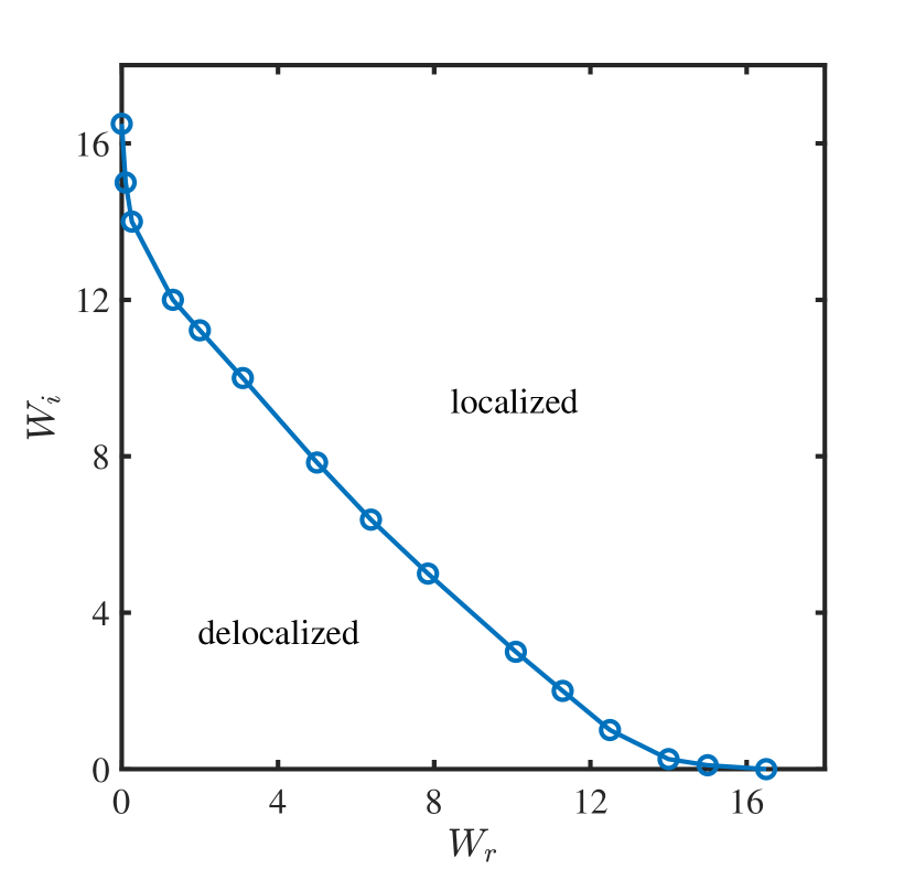
(a) Phase diagram at $E=0$

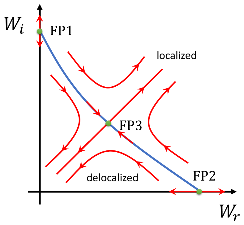
(b) RG flow at $E=0$

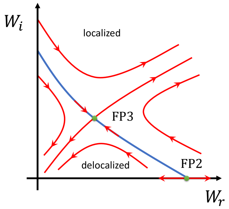
(c) RG flow at $E\neq 0$

Figure 1: (a) $E=0$ phase diagram of the NH Anderson model determined by the localization length, (b) $E=0$ and (c) $E\neq 0$ renormalization group (RG) flow diagram for the NH Anderson model, where $W_{r}$ and $W_{i}$ are the disorder strength for the real and imaginary parts of the complex-valued on-site random potentials, respectively. In (b) and (c), the red curves with arrows stand for the RG flow, the green dots for fixed points (FP) of the RG flow, and the blue line is a phase boundary between delocalized and localized phases. Note that the phase boundary and the RG flow is completely symmetric about a $W_{r}=W_{i}$ line in (a) and (b). We also note that $E\neq 0$ in (c) means that $E$ is real.

• The critical exponents of the NH Anderson, U(1) and Peierls models are accurately determined. The results unambiguously conclude that the critical exponent of the NH class-AI^† (Anderson) is $\nu=1.19\pm 0.01$ and the critical exponent of the NH class A (U(1) and Peierls) is $\nu=1.00\pm 0.04$. These high precision estimates enable us to distinguish the NH class A and NH class AI^†, which was impossible for the previous level statistics study [56]. This supports a strong relation between the universality classes of the Anderson transition and symmetry classification in the NH disordered systems. More importantly, they are distinctly different from the critical exponents in the corresponding universality classes in the Hermitian limit; $\nu=1.572\pm 0.003$ in the orthogonal class [63] (Hermitian class AI) and $\nu=1.443\pm 0.003$ in unitary class (Hermitian class A)  [64, 65].

• Critical properties at different single-particle energy $E$ and system parameters are clarified in the NH Anderson model. This gives phase diagrams in a two-dimensional plane subtended by the disorder strength of the real part of the on-site random potential ($W_{r}$) and that of the imaginary part ($W_{i}$). Especially at the zero single-particle energy ($E=0$), the phase diagram as well as the critical properties across the phase boundary becomes completely symmetric with respect to an exchange of $W_{r}$ and $W_{i}$; Fig. 1(a). The symmetric structure at $E=0$ is a generic feature in any NH bipartite-lattice models with the on-site NH random potentials. Based on the results, we propose a renormalization group (RG) flow diagram in the two-dimensional plane at $E=0$; Fig. 1(b). At $E\neq 0$, the symmetry of the phase diagram and the critical properties is absent; see the RG flow diagram in Fig. 1(c).

• The validity of the transfer matrix analyses in these 3D NH models as well as the 1D Hatano-Nelson model is clarified and demonstrated numerically. The presence or absence of the reciprocal symmetries in Lyapunov exponents and conductance are clarified in the three NH models. Based on a physically reasonable definition of the two-terminal conductance, we show numerically that a conductance distribution is not Gaussian, but it contains small numbers of extremely large conductance values due to rare events of strong amplifications by the NH disorders. We also demonstrate that the geometric mean of the conductance enables a feasible finite-size scaling (FSS) analysis and the results from the FSS analysis give the critical exponents consistent with those values by the localization length.

The organization of this paper is as follows. In the following section, we introduce the three NH models and argue the validity of the transfer matrix analyses. We show the presence or absence of the reciprocal symmetries in the Lyapunov exponents and two-terminal conductance. In Sec. III, we clarify the critical properties of the Anderson transition at different single-particle energies and system parameters in the NH Anderson models together with an accurate estimate of the critical exponent of the NH class AI^†. In Sec. IV, we clarify the critical properties of the Anderson transition in two NH class A models, i.e., U(1) and Peierls models, together with an estimate of the critical exponent of the NH class A. In Sec. V, we compare the transfer matrix analyses with the level statistics analyses[54, 56] and describe a possible reason for a discrepancy of the critical exponent of the NH class AI^† between the two analyses. The final section is devoted to summary and concluding remarks.

II numerical method

We study the following tight-binding models defined on a 3D cubic lattice,

$${\cal H}=\sum_{\bm{i}}\varepsilon_{\bm{i}}c^{\dagger}_{\bm{i}}c_{\bm{i}}+\sum_{\langle{\bm{i}},{\bm{j}}\rangle}e^{2\pi{\rm i}\theta_{{\bm{i}},{\bm{j}}}}c^{\dagger}_{\bm{i}}c_{\bm{j}}\equiv\sum_{{\bm{i}},{\bm{j}}}c^{\dagger}_{\bm{i}}(\mathbb{H})_{{\bm{i}},{\bm{j}}}c_{\bm{j}},$$ (1)

where $c^{\dagger}_{\bm{i}}$ ($c_{\bm{i}}$) is the creation (annihilation) operator. $\bm{i}$ and $\bm{j}$ specify the cubic lattice site; ${\bm{i}}=(i_{x},i_{y},i_{z})$ and $i_{\mu}=1,2,\cdots,L_{\mu}$ ($\mu=x,y,z$). The models have Hermitian hoppings between nearest neighbor sites in the cubic lattice; $\langle{\bm{i}},{\bm{j}}\rangle$ means that $\bm{i}$ and $\bm{j}$ are the nearest neighbor sites with $\theta_{{\bm{i}},{\bm{j}}}=-\theta_{{\bm{j}},{\bm{i}}}$. The model is the Anderson model for $\theta_{{\bm{i}},{\bm{j}}}$ = 0 and the U(1) model with a random number $\theta_{{\bm{i}},{\bm{j}}}$ in a range of $[0,1)$ [66, 64]. When $\theta_{{\bm{i}},{\bm{j}}}=\Phi\!\ i_{x}$ for ${\bm{j}}={\bm{i}}+{\bm{e}}_{z}$, the model is the Peierls model [67, 68], where $2\pi\Phi$ is a magnetic gauge flux that penetrates through every square plaquette in the $z$-$x$ plane of the cubic lattice. In this paper, we study the Anderson transition driven by random complex on-site potentials, $\varepsilon_{\bm{i}}=w^{r}_{\bm{i}}+{\rm i}\!\ w^{i}_{\bm{i}}$ with the imaginary unit ${\rm i}$, where $w^{r}_{\bm{i}}$ and $w^{i}_{\bm{i}}$ are independent random numbers with the uniform distribution in a range of $[-W_{r}/2,W_{r}/2]$ and $[-W_{i}/2,W_{i}/2]$, respectively. Hence ${\cal H}^{\dagger}\neq{\cal H}$, where the non-zero $w^{r}_{\bm{i}}$ and $w^{i}_{\bm{i}}$ bring about the non-Hermiticity in the system. According to the symmetry classification, the Anderson model ($\theta_{{\bm{i}},{\bm{j}}}=0$) belongs to 3D NH class AI^† and the U(1) and Peierls models ($\theta_{{\bm{i}},{\bm{j}}}\neq 0$) belong to 3D NH class A. The time reversal symmetry (TRS) is broken (${\cal H}^{*}\neq{\cal H}$) in both classes, whereas the transposition symmetry (${\cal H}^{\mathrm{T}}={\cal H}$), namely TRS^†, holds true in the class AI^†[16, 69]. We note that not only a parameter region of $W_{i}=0$ but also a parameter region of $W_{r}=0$ and $E=0$ belong to the Hermitian universality class in these three NH models (Sec. III).

Transfer matrix method are widely used both in the Hermitian [70, 71, 72, 73] and non-Hermitian [74, 75, 76, 77, 78, 79, 80, 81, 82, 83, 84] systems. In order to study the Anderson transition of eigenstates of ${\cal H}$ with a complex-valued eigenenergy $E$, the quasi-1D localization length (Lyapunov exponent) and two-terminal conductance in cubic systems are evaluated by the transfer matrix method at the energy $E$ for different system sizes. The quantities are further analyzed by the finite size scaling, which determines the critical properties of the Anderson transition in the NH systems. Although the transfer matrix method has been widely used in the non-Hermitian optical systems during last several decades, the transfer matrix analysis on the Anderson transitions in non-Hermitian systems has not been carried out prior to this work. Thus, we first clarify the nature of the Lyapunov exponent and the two-terminal conductance in the NH systems studied in this paper as well as pseudo-Hermitian systems.

II.1 transfer matrix method

In the transfer matrix method, the 3D $L_{x}\times L_{y}\times L_{z}(=N)$ cubic lattice is regarded as a multiple-layer structure of its two-dimensional (2D) slices, where the 2D slice is in the $x$-$y$ plane of the cubic lattice and the slices are stacked along $z$. An eigenvalue problem of the $N\times N$ disordered NH Hamiltonian reduces to a set of linear equations relating the wavefunction on the adjacent slices. The equation takes a form of a matrix multiplication of a transfer matrix that connects the wavefunctions on the adjacent slices[70, 71, 72, 85, 86, 73],

$$\begin{pmatrix}\psi_{i_{z}+1}\\ V_{i_{z}+1,i_{z}}\psi_{i_{z}}\end{pmatrix}=M_{i_{z}}\begin{pmatrix}\psi_{i_{z}}\\ V_{i_{z},i_{z}-1}\psi_{i_{z}-1}\end{pmatrix},$$ (2)

where $\psi_{i_{z}}$ is the wavefunction on the slice at position $i_{z}$. $M_{i_{z}}$ is the transfer matrix defined by,

$$M_{i_{z}}=\begin{pmatrix}V_{i_{z},i_{z}+1}^{-1}(E-H_{i_{z}})&-V_{i_{z},i_{z}+1}^{-1}\\ V_{i_{z}+1,i_{z}}&0\end{pmatrix},$$ (3)

$V_{i_{z}+1,i_{z}}$ is a hopping term matrix between the slice at $i_{z}+1$ and that at $i_{z}$. In Eq. (1), $V_{i_{z}+1,i_{z}}$ is a $L_{x}L_{y}$ by $L_{x}L_{y}$ diagonal matrix whose diagonal elements have the unit modulus. Note that for NH U(1) model, we use local gauge transformation to eliminate the phase of the hopping along $z$-direction. $H_{i_{z}}$ consists of a hopping term and diagonal term within the slice at $i_{z}$. In Eq. (1), the diagonal elements of $H_{i_{z}}$ are the complex-valued on-site potentials, and off-diagonal elements are the nearest neighbor hoppings within the slice. The localization length and two-terminal conductance are calculated along $z$ with either periodic boundary conditions (PBC) or open boundary conditions (OBC) in the transverse direction, $x$ and $y$.

II.1.1 localization length

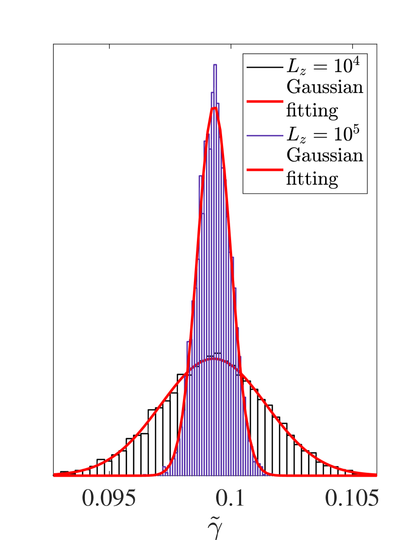
(a) Anderson model

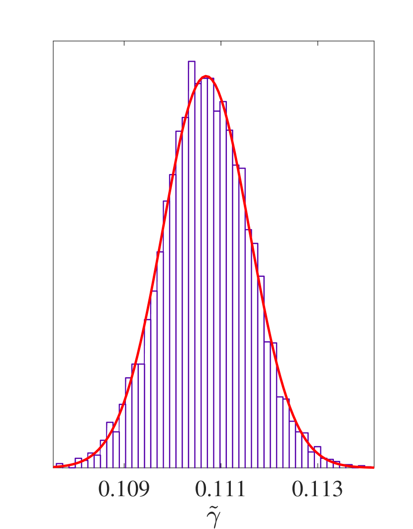
(b) U(1) model

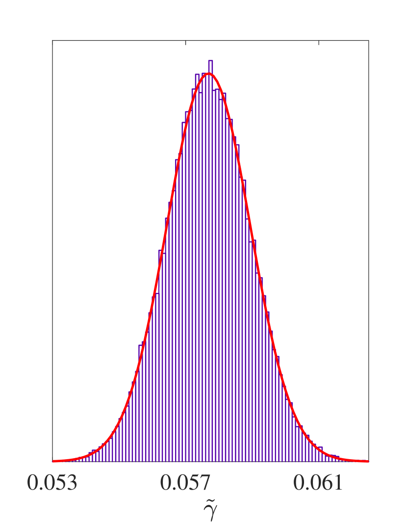
(c) Hatano-Nelson model

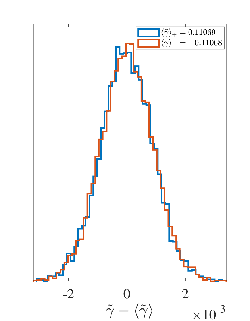
(d) U(1) model

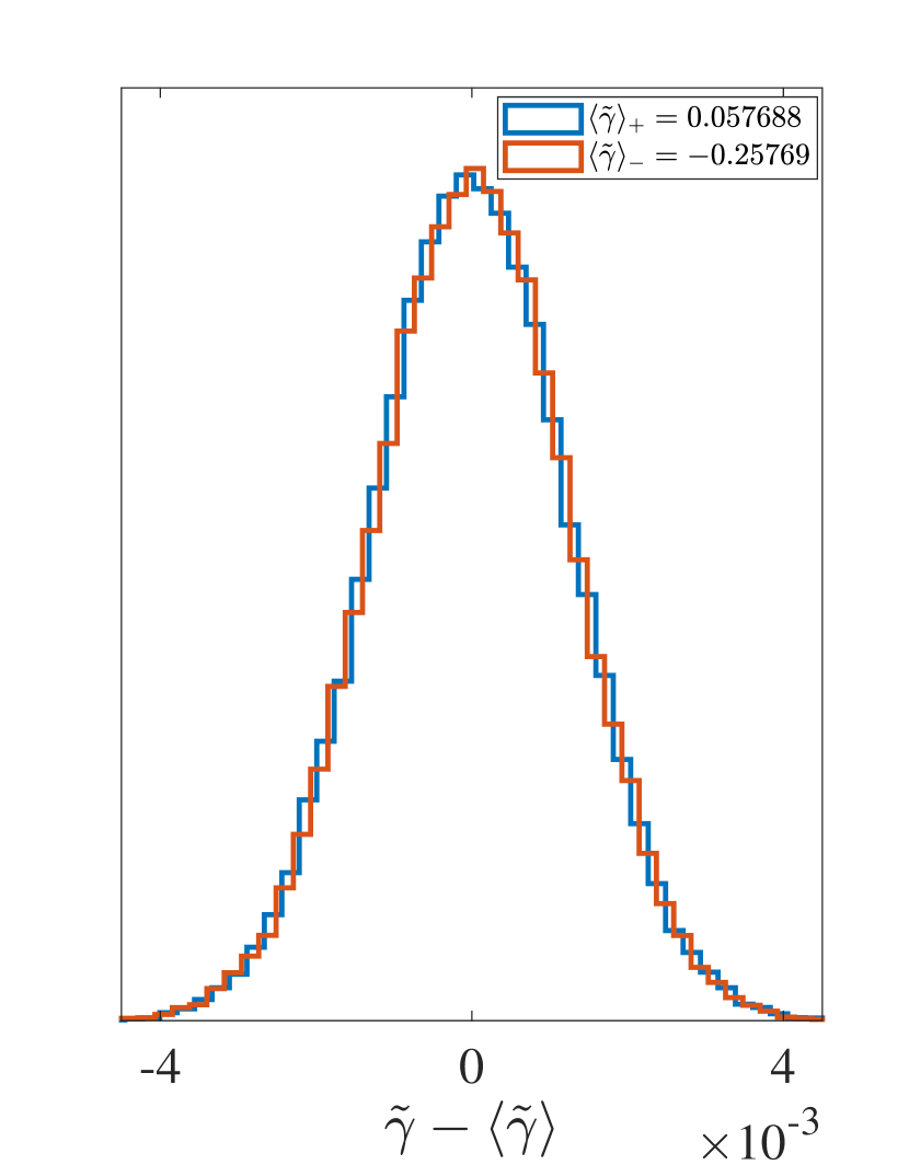
(e) Hatano-Nelson model

Figure 2: Histograms of the Lyapunov exponent $\tilde{\gamma}$ estimated from finite $L_{z}$. For (a)-(c), $\tilde{\gamma}$ stands for the the smallest positive Lyapunov exponent. For (d) and (e), $\langle\tilde{\gamma}\rangle_{+}$ is the smallest positive Lyapunov exponent and $\langle\tilde{\gamma}\rangle_{-}$ is the largest negative Lyapunov exponent. (a) NH Anderson model with $W_{r}=W_{i}=6.2$, (b) and (d) NH U(1) model with $W_{r}=W_{i}=7$. The data of (a), (b), (d) come from $6400$ realizations of disordered systems with independent random number with $L_{x}=L_{y}=L=10$ and $L_{z}=10^{5}$ (also $L_{z}=10^{4}$ in (a)) at $E=0$. (c) and (e) 1D Hatano-Nelson model with $g=0.1$ and $W=4$, $64000$ realizations of disordered systems with $L_{z}=10^{5}$ at $E=0$. The red curves in (a)-(c) are the Gaussian fittings.

We consider transmission of particles of a complex-valued energy $E$ through long disordered wire ($L_{x},L_{y}\ll L_{z}$) with a square cross-section $L_{x}=L_{y}=L$. For the long wire, the amplitude of the transmission decays exponentially with an associated decay length called the quasi-1D localization length $\lambda$. To calculate $\lambda$, we consider a product of the transfer matrix over the layer from $i_{z}=1$ to $i_{z}=L_{z}$. The product relates the wavefunctions at $i_{z}=0,1$ and those at $i_{z}=L_{z},L_{z}+1$;

$$M=\prod_{i_{z}=1}^{L_{z}}M_{i_{z}}.$$ (4)

For the product of random matrices such as $M_{i_{z}}$, some eigenvalues of the product decay exponentially in $L_{z}$, while the others grow exponentially in $L_{z}$. The simultaneous emergence of the eigenvalues with the exponential decay and growth represents a reciprocal symmetry nature of the 3D NH systems. The reciprocal symmetry in the NH Anderson model is protected by the transposition symmetry ${\cal H}^{\mathrm{T}}={\cal H}$ in each disorder realization, while it is not the case in the NH U(1) and Peierls models. Nonetheless, the reciprocal symmetry in the latter two models appears asymptotically in the thermodynamic limit $L_{z}\rightarrow\infty$, where the transposition symmetry (Hermitian symmetry) is effectively restored after an average over $i_{z}$ from $i_{z}=0$ to $i_{z}=L_{z}$; the transposition symmetry (Hermitian symmetry) exists statistically in the NH U(1) (Peierls) models.

The amplitude part of the complex-valued eigenvalue of $M$ with the slowest exponentially decay (growth) defines the quasi-1D localization length of the system with the long-wire geometry. To extract this length, it is convenient to consider a positive-semi-definite Hermitian matrix $MM^{\dagger}$, and its logarithm,

$$\Omega=\ln MM^{\dagger}.$$ (5)

When ${\cal H}$ is Hermitian, $\Omega$ satisfies the Oseledec’s theorem[87, 88]. The theorem dictates that in the limit of large $L_{z}$, eigenvalues of $\Omega/L_{z}$ obtained from the product of random matrices $M_{i_{z}}$ ($i_{z}=1,\cdots,L_{z}$) converges to non-random numbers. Any matrix product of $n\times n$ complex-valued matrices is equivalent to $2n\times 2n$ real-valued matrices, because a product of two complex numbers $z_{1}=x_{1}+{\rm i}y_{1}$ and $z_{2}=x_{2}+{\rm i}y_{2}$ can be regarded as a matrix product of two real-valued 2 by 2 matrices $x_{1}\tau_{0}+{\rm i}y_{1}\tau_{y}$ and $x_{2}\tau_{0}+{\rm i}y_{2}\tau_{y}$. Thereby, $\Omega/L_{z}$ obtained from the non-Hermitian random ${\cal H}$ also satisfies the Oseledec’s theorem [89]. According to the theorem, eigenvalues of $\Omega$ decrease (increase) linearly in the large $L_{z}$. The Lyapunov exponents $\gamma_{i}$ are defined by the eigenvalues of $\Omega$, $\nu_{i}$,

$$\gamma_{i}\equiv\frac{\nu_{i}}{2L_{z}}$$ (6)

for $i=1,2,\cdots,2L_{x}L_{y}$.

In the NH Anderson model, the positive Lyapunov exponents and negative Lyapunov exponents appear in pairs,

$$\{\cdots,\gamma_{3},\gamma_{2},\gamma_{1},-\gamma_{1},-\gamma_{2},-\gamma_{3},\cdots\},$$

with $\cdots>\gamma_{2}>\gamma_{1}>0>-\gamma_{1}>\cdots$ because of the transposition symmetry of the transfer matrix;

$$\sigma_{y}M^{\mathrm{T}}_{i_{z}}\sigma_{y}=M^{-1}_{i_{z}},$$ (7)

for any $i_{z}$. The symmetry relates a pair of the two eigenvalues $\{\nu_{i},-\nu_{i}\}$ in any finite $L_{z}$ through $\sigma_{y}(MM^{\dagger})^{\mathrm{T}}\sigma_{y}=(MM^{\dagger})^{-1}$. In the NH U(1) model, the transpositional symmetry holds between $M_{i_{z}}$ from ${\cal H}$ and $M_{i_{z}}$ from ${\cal H}^{\mathrm{T}}$;

$$\sigma_{y}M_{i_{z}}^{\mathrm{T}}({\cal H})\sigma_{y}=M_{i_{z}}^{-1}({\cal H}^{\mathrm{T}}).$$ (8)

Thus, the positive (negative) Lyapunov exponents from ${\cal H}$ and the negative (positive) Lyapunov exponents from ${\cal H}^{\mathrm{T}}$ are related to each other;

$$\{\cdots,\gamma_{3},\gamma_{2},\gamma_{1},-\gamma^{\prime}_{1},-\gamma^{\prime}_{2},-\gamma^{\prime}_{3},\cdots\}$$

from ${\cal H}$ with $\cdots>\gamma_{2}>\gamma_{1}>0>-\gamma^{\prime}_{1}>\cdots$ and

$$\{\cdots,\gamma^{\prime}_{3},\gamma^{\prime}_{2},\gamma^{\prime}_{1},-\gamma_{1},-\gamma_{2},-\gamma_{3},\cdots\}$$

from ${\cal H}^{\mathrm{T}}$ with $\cdots>\gamma^{\prime}_{2}>\gamma^{\prime}_{1}>0>-\gamma_{1}>\cdots$. Since ${\cal H}$ and ${\cal H}^{\mathrm{T}}$ appear with an equal probability in the NH U(1) model, $\gamma_{i}=\gamma^{\prime}_{i}$ holds true in the thermodynamic limit ($L_{z}\rightarrow\infty$). The same holds true in the NH Peierls model, in which ${\cal H}$ and ${\cal H}^{\dagger}$ appear with an equal probability. Finally, the reciprocal of the smallest positive Lyapunov exponent $\gamma_{1}$ is nothing but the quasi-1D localization length

$$\lambda=1/\gamma_{1}=2L_{z}/\nu_{1}.$$ (9)

To check the stability of the estimate of the Lyapunov exponents in the NH systems by the transfer matrix method, we estimate the Lyapunov exponents with finite $L_{z}$ in repeated simulations with the same parameters with an independent stream of random numbers. In practice, the Lyapunov exponents are calculated by $QR$ decomposition [73] instead of by diagonalizing the matrix $\Omega$. Fig. 2 shows distributions of the Lyapunov exponents in the NH Anderson and U(1) models as well as 1D Hatano-Nelson model [57]. The distributions are always Gaussian, indicating the stability of the evaluations of the Lyapunov exponents from the transfer matrix method. Moreover, the standard deviation of the Gaussian distribution becomes smaller with larger $L_{z}$ [Fig. 2(a)], which indicates that Lyapunov exponent will converge to a constant in the large $L_{z}$ limit. The Lyapunov exponents in the NH Anderson model come in pair protected by symmetry. In the NH U(1) and Peierls models, the smallest positive Lyapunov exponent and the largest negative Lyapunov exponent are consistent with each other in sufficiently large $L_{z}$ [Fig. 2(d)]. On the one hand, they are distinct from each other even in the large $L_{z}$ in the 1D Hatano-Nelson model [Fig. 2(e)], where both Hermitian symmetry and transposition symmetry are broken even statistically. In the 1D Hatano-Nelson model, rightward-decaying eigenfunctions and leftward-decaying eigenfunctions have different longest decay lengths due to asymmetric hopping terms; $e^{g}$ for rightward hopping term and $e^{-g}$ for leftward hopping term.

II.1.2 conductance

The two-terminal conductance can be also formulated for the NH systems in the same framework as the scattering theory in Hermitian systems [90, 91]. Thereby, the 3D $L_{x}\times L_{y}\times L_{z}$ cubic lattice is regarded as a scattering object and the two-terminal conductance is defined as a total number of particles that transmit through the scattering object within a unit time and within a unit energy window. To calculate the conductance, we consider that the disordered system with a cross-section of $L_{x}L_{y}$ and a length of $L_{z}$ is attached to two leads. Each lead comprises of $2L_{x}L_{y}$ decoupled 1D wires, half of which have right-moving current flux along $+z$ direction and the other half have left-moving current flux along $-z$. For simplicity, we regard the two leads as the Hermitian system and identify all the $L_{x}L_{y}$ 1D wires with the left(right)-moving flux as eigenstates of the following 1D tight-binding model

$${\cal H}_{\rm lead}=\sum_{i_{z}}c^{\dagger}_{(i_{x},i_{y},i_{z}+1)}c_{(i_{x},i_{y},i_{z})}+{\rm h.c.}.$$ (10)

The left (right)-moving current flux states are regarded as eigenstates at right (left) ‘Fermi’ points of the 1D tight-binding model respectively. Such states are given by $e^{-{\rm i}k_{z}i_{z}}$ and $e^{{\rm i}k_{z}i_{z}}$ with their (real-valued) eigen-energy $E=2\cos k_{z}$ and $k_{z}\in[-\pi,\pi)$.

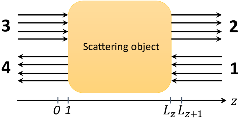
Figure 3: Two-terminal conductance geometry. 1 and 3 represent the incoming current flux; 2 and 4 represent the outgoing current flux.

The scattering object is characterized by a scattering matrix $S$ among right-moving current fluxes and left-moving fluxes in the two leads[92];

$$\left(\begin{array}[]{c}2\\ 4\\ \end{array}\right)=\left(\begin{array}[]{cc}r&t^{\prime}\\ t&r^{\prime}\\ \end{array}\right)\left(\begin{array}[]{c}1\\ 3\\ \end{array}\right)\equiv S\left(\begin{array}[]{c}1\\ 3\\ \end{array}\right).$$ (19)

Here $1$ ($2$) and $4$ ($3$) represent $L_{x}L_{y}$ vectors for the left (right)-moving fluxes in the right lead and in the left lead, respectively (Fig. 3). Four $L_{x}L_{y}\times L_{x}L_{y}$ matrices in $S$, $t$, $t^{\prime}$, $r$ and $r^{\prime}$, are the transmission matrix from right to left, the transmission matrix from left to right, the reflection matrix in the right lead, and the reflection matrix in the left lead, respectively. Due to the reciprocal symmetry, the scattering matrix is symmetric ($S^{\mathrm{T}}=S$) in the NH Anderson model, while they are not in the NH U(1) and NH Peierls models.

In the NH U(1) and Peierls models, the transposition of the Hamiltonian changes the sign of the external magnetic fluxes $\{\Phi\}$, where $\{\Phi\}$ indicates the position dependent magnetic fluxes in the U(1) model whereas it is constant in the Peierls model. Thereby, the leftward conductance and rightward conductance defined below do not coincide with each other in general for a nonzero $\{\Phi\}$.

$$g_{L} \equiv{\rm Tr}[tt^{\dagger}],$$

$$g_{R} \equiv{\rm Tr}[t^{\prime}{t^{\prime}}^{\dagger}].$$

Nonetheless, $S^{\mathrm{T}}({\cal H}_{\{\Phi\}})=S({\cal H}^{\mathrm{T}}_{\{\Phi\}})=S({\cal H}_{\{-\Phi\}})$ indicates that leftward (rightward) conductance with the magnetic fluxes ${\{\Phi\}}$ is the same as the rightward (leftward) conductance with the flux ${\{-\Phi\}}$ in the NH U(1)/Peierls models;

$$g_{R/L}({\{\Phi\}})=g_{L/R}({-\{\Phi\}}).$$ (20)

To calculate the transmission matrix $t$ by the transfer matrix method, we rewrite the scattering matrix into a matrix $T$. $T$ connects the left lead to the right lead;

$$\left(\begin{array}[]{c}1\\ 2\\ \end{array}\right)=\left(\begin{array}[]{cc}t^{-1}&-t^{-1}r^{\prime}\\ rt^{-1}&-rt^{-1}r^{\prime}+t^{\prime}\\ \end{array}\right)\left(\begin{array}[]{c}4\\ 3\\ \end{array}\right)\equiv T\left(\begin{array}[]{c}4\\ 3\\ \end{array}\right),$$ (29)

The product of the transfer matrix, $M$, relates wavefunction amplitudes of ${\cal H}$ in the left and the right leads. Thereby, by the use of $M$, the eigenstates of ${\cal H}_{{\rm lead}}$ (the left lead) with the two opposite current flux can be generalized into the eigenstates of ${\cal H}+{\cal H}_{\rm lead}$. The two eigenstates thus obtained take the following forms at the beginning of the right lead ($i_{z}=L_{z}+1,L_{z}$);

$$\left(\begin{array}[]{c}\psi_{L_{z}+1}\\ \psi_{L_{z}}\\ \end{array}\right) =M\frac{1}{\sqrt{2}}\left(\begin{array}[]{c}e^{{\rm i}k_{z}}\\ 1\\ \end{array}\right)\otimes{\bm{e}}_{i},$$ (34)

$$\left(\begin{array}[]{c}\psi_{L_{z}+1}\\ \psi_{L_{z}}\\ \end{array}\right) =M\frac{1}{\sqrt{2}}\left(\begin{array}[]{c}1\\ e^{{\rm i}k_{z}}\\ \end{array}\right)\otimes{\bm{e}}_{i},$$ (39)

with $k_{z}>0$ and $i=1,2,\cdots,n$, $n$ being $L_{x}L_{y}$. Here we note that $V_{i_{z}+1,i_{z}}$ in Eq. (2) is an $n$-dimensional unit matrix for the NH Anderson and U(1) models and ${\bm{e}}_{i}$ is an $n$-dimensional unit vector associated with $x$ and $y$ coordinates. In the following, we will omit the $x$-$y$ coordinate degree of freedom unless dictated explicitly.

The matrix $T$ is given by an inner product between the two eigenstates of ${\cal H}+{\cal H}_{\rm lead}$ and the two eigenstates of the right-lead Hamiltonian;

$$T\equiv\frac{1}{2}\left(\begin{array}[]{cc}1&e^{-{\rm i}k_{z}}\\ e^{-{\rm i}k_{z}}&1\\ \end{array}\right)\Sigma M\left(\begin{array}[]{cc}1&e^{{\rm i}k_{z}}\\ e^{{\rm i}k_{z}}&1\\ \end{array}\right).$$ (44)

The inner products are taken at $i_{z}=L_{z}+1,L_{z}$ with a matrix $\Sigma$. When all the $H_{i_{z}}$ in $M$ are set to zero, the scattering object becomes identical to the two leads. Thereby, the $T$ matrix at $E=2\cos k_{z}$ must be proportional to a diagonal matrix with diagonal elements of the unit modulus. This requirement defines the inner product with a proper normalization[90, 93];

$$T \equiv\frac{1}{2\sin k_{z}}\left(\begin{array}[]{cc}1&e^{-{\rm i}k_{z}}\\ e^{-{\rm i}k_{z}}&1\\ \end{array}\right)\sigma_{y}M\left(\begin{array}[]{cc}1&e^{{\rm i}k_{z}}\\ e^{{\rm i}k_{z}}&1\\ \end{array}\right).$$ (49)

For the Hermitian system, the symplectic nature of the transfer matrix guarantees the unitarity of the scattering matrix[92]. Namely, $\sigma_{y}M^{\dagger}\sigma_{y}=M^{-1}$ leads to $\sigma_{z}T^{\dagger}\sigma_{z}=T^{-1}$ and $S^{\dagger}=S^{-1}$.

In the NH Anderson model, the transfer matrix only has a pseudo-symplectic nature, Eq. (7). The pseudo-symplecticy of the transfer matrix imposes the pseudo-symplecticy on $T$ and the symmetric nature on the $S$ matrix respectively;

$$\sigma_{y}T^{\mathrm{T}}\sigma_{y}=T^{-1},\!\ S^{\mathrm{T}}=S.$$ (50)

The symmetric $S$ matrix leads to the reciprocal symmetry in the conductance; $g_{R}=g_{L}$. In the NH U(1) model, the pseudo-symplecticy holds true only between ${\cal H}$ and ${\cal H}^{\mathrm{T}}$. So does the symmetric nature of the $S$ matrix;

$$S^{\mathrm{T}}({\cal H})=S({\cal H}^{\mathrm{T}}).$$ (51)

Since ${\cal H}$ and ${\cal H}^{\mathrm{T}}$ appear with equal probability in the NH U(1) model, eq. (51) leads to the reciprocal symmetry in the averaged conductance in the NH U(1) model; $\langle g_{R}\rangle=\langle g_{L}\rangle$. Thereby, for the NH Anderson and U(1) models, we have only to define the two-terminal conductance by one of the two transmission matrices;

$$g\equiv\langle{\rm Tr}[tt^{\dagger}]\rangle.$$ (52)

In the NH Peierls model where the magnetic field is uniform, $g_{R}$ and $g_{L}$ are different.

Note that in the three NH models, the non-Hermiticity is introduced only by the on-site NH disorder potential, $w_{\bm{i}}^{r}$ and $w_{\bm{i}}^{i}$, which range in $[-W_{r}/2,W_{r}/2]$ and $[-W_{i}/2,W_{i}/2]$, respectively. Thereby, the Hermiticity is recovered statistically; ${\cal H}^{\dagger}$ and ${\cal H}$ realize with equal probability in an ensemble of many disorder realizations. Nonetheless, $S^{\dagger}({\cal H})=S^{-1}({\cal H}^{\dagger})$ does not guarantee the unitarity of the scattering matrix in any way, e.g. even after the disorder average,

$$\langle r^{\dagger}r\rangle+\langle t^{\dagger}t\rangle\neq{\mathbb{1}}_{L_{x}L_{y}\times L_{x}L_{y}}.$$ (53)

On the contrary, $S^{\dagger}({\cal H})=S^{-1}({\cal H}^{\dagger})$ gives

$$r^{\dagger}({\cal H})r({\cal H}^{\dagger})+t^{\dagger}({\cal H})t({\cal H}^{\dagger})={\mathbb{1}}_{L_{x}L_{y}\times L_{x}L_{y}}.$$ (54)

This suggests that the conductance $g$ in the NH systems is not bounded by the total number of the transmission channels, i.e., $n=L_{x}L_{y}$. This is in some sense physically reasonable because the transmission amplitude in the NH systems can be amplified by the on-site NH disorder potentials, when particles going through the scattering object.

II.1.3 Lyapunov exponent and scattering matrix in non-Hermitian systems with pseudo-Hermiticity

Transfer matrix method has been extensively used in ${\cal PT}$-symmetric non-Hermitian optical systems [74, 78, 79, 75, 80, 81, 82, 43, 84, 76, 94, 95, 96, 97, 77, 98] as well as pseudo-Hermitian magnon systems [51]. The ${\cal PT}$-symmetric systems can be regarded as non-Hermitian system with pseudo-Hermiticity [99, 100]. In this section, we summarize reciprocal symmetry of the Lyapunov exponents and symmetry properties of the scattering matrix in non-Hermitian disordered systems with pseudo-Hermiticity. The symmetry properties of the scattering matrix have been previously discussed in the ${\cal PT}$ symmetric optical systems in the context of perfect coherent absorber [76, 94, 95, 96, 97, 77, 98], and 1D NH class AI (Hatano-Nelson model) [101].

Hamiltonian $\mathbb{H}$ with the pseudo-Hermiticity,

$$\eta{\mathbb{H}}\eta^{-1}={\mathbb{H}}^{\dagger},$$ (55)

is introduced in an eigenvalue problem on a 3D cubic lattice,

$$\mathbb{H}\Psi=E\Psi.$$ (56)

The argument can be easily generalized into other lattices. Here $\eta$ is Hermitian and unitary matrix; $\eta^{\dagger}\eta=\eta\eta^{\dagger}=1$ and $\eta^{\dagger}=\eta$. We allow $\mathbb{H}$ to have internal degrees of freedom, such as spin, sublattice, and particle-hole degrees of freedom. For example, generalized eigenvalue problems for free quasi-particle boson systems are equivalent to diagonalizing pseudo-Hermitian Hamiltonian [102, 103, 16, 104]. Thereby, the internal degree of freedom is particle-hole degree of freedom of the boson, $\Psi$ is a Nambu vector subtended by both boson creation and annihilation operators and $\eta$ is given by a diagonal matrix that takes $+1/-1$ for the creation/annihilation operators [102, 103]. As above, 3D $L_{x}\times L_{y}\times L_{z}$ cubic lattice is regarded as the multiple layer structure of the two-dimensional (2D) slices. Without loss of generality, we can assume that $\mathbb{H}$ has hoppings only between the nearest neighboring 2D slices,

$$\mathbb{H}=\left(\begin{array}[]{cccc}\ddots&V_{i_{z}-1,i_{z}}&0&\\ V_{i_{z},i_{z}-1}&H_{i_{z}}&V_{i_{z},i_{z}+1}&0\\ 0&V_{i_{z}+1,i_{z}}&H_{i_{z}+1}&V_{i_{z}+1,i_{z}+2}\\ &0&V_{i_{z}+2,i_{z}+1}&\ddots\\ \end{array}\right).$$ (61)

$H_{i_{z}}$ includes on-site disorder potentials and hopping integrals within the 2D slice at $i_{z}$. $V_{i,j}$ are hopping integrals between 2D slice at $i$ and 2D slice at $j$, which we assume to be any invertible $L_{x}L_{y}\times L_{x}L_{y}$ matrix. In the presence of the on-site disorder in $H_{i_{z}}$, a Hermitian matrix $\eta$ that satisfies Eq. (55) must be diagonal with respect to the site index ${\bm{i}}=(i_{x},i_{y},i_{z})$. Accordingly, the transfer matrix in Eq. (3) has the following symmetry,

$$\eta\sigma_{y}M^{\dagger}_{i_{z}}(E)\sigma_{y}\eta^{-1}={M_{i_{z}}(E^{*})}^{-1}$$ (62)

with complex-valued eigen-energy $E$. This results in the reciprocal symmetry between the Lyapunov exponents at $E$ and $E^{*}$;

$$\{\cdots,\gamma_{2}(E),\gamma_{1}(E),-\gamma^{\prime}_{1}(E),-\gamma^{\prime}_{2}(E),\cdots\}$$

with $\gamma_{i}(E^{*})=\gamma^{\prime}_{i}(E)$, $\cdots>\gamma_{2}>\gamma_{1}>0>-\gamma^{\prime}_{1}>-\gamma^{\prime}_{2}>\cdots$. For real-valued $E$, $\gamma^{\prime}_{i}(E)=\gamma_{i}(E)$. Based on this reciprocal relation, Ref. [51] previously studied quantum magnon Hall plateau transition, clarifying that the universality class of the plateau transition in the pseudo-Hermitian systems belongs to the same universality class as the Hermitian quantum Hall plateau transition. Eq. (62) also dictates that the scattering matrix defined in Eqs. (19), (29), and (49) has unitarity-like relation between $E$ and $E^{*}$; $S^{\dagger}(E)\eta S(E^{*})=\eta$.

The pseudo-Hermiticity allows time-independent inner product between two wavefunctions in the Schrodinger picture; $\partial_{t}(\langle\Psi(t)|\eta|\Psi(t)\rangle)=0$ with $\mathbb{H}|\Psi(t)\rangle=i\partial_{t}|\Psi(t)\rangle$. Such an inner product represents conserved (local) physical quantities of underlying physical systems. In the example of the generalized eigenvalue problems for quasi-particle boson systems, the inner product corresponds to an energy density carried by the bosons [105, 106, 51, 104]. Thus, the transfer matrix method in such pseudo-Hermitian systems should be reformulated in such a way that the conservation rule becomes explicit in the transport properties. To this end, it is more natural to introduce the transfer matrix as [51]

$$\tilde{M}_{i_{z}}=\begin{pmatrix}\tilde{V}_{i_{z},i_{z}+1}^{-1}(E\eta-\tilde{H}_{i_{z}})&-\tilde{V}_{i_{z},i_{z}+1}^{-1}\\ \tilde{V}_{i_{z}+1,i_{z}}&0\end{pmatrix},$$ (63)

with

$$\tilde{\mathbb{H}}\equiv\eta\mathbb{H}\equiv\left(\begin{array}[]{cccc}\ddots&\tilde{V}_{i_{z}-1,i_{z}}&&\\ \tilde{V}_{i_{z},i_{z}-1}&\tilde{H}_{i_{z}}&\tilde{V}_{i_{z},i_{z}+1}&\\ &\tilde{V}_{i_{z}+1,i_{z}}&\tilde{H}_{i_{z}+1}&\tilde{V}_{i_{z}+1,i_{z}+2}\\ &&\tilde{V}_{i_{z}+2,i_{z}+1}&\ddots\\ \end{array}\right),$$ (68)

and calculate $T$-matrix and scattering matrix according to Eqs. (19,29,49) with $M$ replaced by $\tilde{M}\equiv\prod_{i_{z}}\tilde{M}_{i_{z}}$. Such scattering matrix respects the unitarity relation, $S^{\dagger}(E)S(E^{*})=\mathbb{1}$, and therefore the conductance for the real-valued $E$ is compatible with the conservation principle. In the example of the free quasi-particle boson systems, the conductance thus calculated is thermal (energy) conductance carried by the quasi-particle bosons [51]. Note also that $\tilde{M}$ gives the same sets of the Lyapunov exponents as $M$, since $\tilde{M}$ and $M$ are related to each other by a unitary transformation.

Before concluding this subsection, we like to emphasize that the models of the NH class A and NH class AI^† studied in this paper do not have ${\cal PT}$-symmetry, but they still have symmetry relations such as Eqs. (7), (8), (20), (50), (51), and (54): see a summary in Table II.

II.2 polynomial fitting

Table 1: Polynomial fitting results for normalized localization length around the Anderson transition point in the presence of the NH disorder with disorder strength $W_{r}$ and $W_{i}$. The goodness of fit (GOF), critical disorder $W_{c}$, critical exponent $\nu$, the scaling dimension of the least irrelevant scaling variable $-y$, and the critical normalized localization length $\Lambda_{c}$ are shown for various system sizes and for different orders of the Taylor expansion: $(m_{1},n_{1},m_{2},n_{2})$. The square bracket is the 95% confidence interval.

Anderson model at $E=0$
disorder	$L$	$m_{1}$	$n_{1}$	$m_{2}$	$n_{2}$	GOF	$W_{c}$	$\nu$	$y$	$\Lambda_{c}$
$W_{r}=W_{i}$	6-24	3	3	0	1	0.10	6.3868[6.3861, 6.3874]	1.190[1.187, 1.193]	2.33[2.22, 2.48]	0.8359[0.8350, 0.8369]
	8-24	3	3	0	1	0.16	6.3858[6.3851, 6.3864]	1.193[1.189, 1.197]	2.57[2.43, 2.72]	0.8375[0.8365, 0.8384]
	10-24	3	3	0	1	0.13	6.3862[6.3852, 6.3872]	1.192[1.185, 1.198]	2.67[2.44, 2.91]	0.8369[0.8353, 0.8385]
$W_{i}=5$	6-16	3	3	0	1	0.12	7.839[7.837, 7.842]	1.194[1.189, 1.199]	2.38[2.25, 2.52]	0.8368[0.8356, 0.8380]
$W_{r}=5$	6-16	3	3	0	1	0.19	7.841[7.838, 7.843]	1.190[1.185, 1.196]	2.37[2.24, 2.57]	0.8361[0.8348, 0.8376]
$W_{i}=0.1$	10-20	3	3	1	1	0.18	14.435[14.414, 14.462]	0.914[0.843, 1.026]	0.99[0.84, 1.25]	0.8442[0.8246, 0.8600]
$W_{r}=0$	4-20	2	3	0	1	0.90	16.543[16.536, 16.550]	1.574[1.567, 1.581]	2.67[2.42, 2.92]	0.5753[0.5742, 0.5763]
	4-20	3	3	0	1	0.90	16.543[16.535, 16.550]	1.569[1.558, 1.578]	2.70[2.46, 2.97]	0.5754[0.5743, 0.5764]
Anderson model at $E={\rm i}$
disorder	$L$	$m_{1}$	$n_{1}$	$m_{2}$	$n_{2}$	GOF	$W_{c}$	$\nu$	$y$	$\Lambda_{c}$
$W_{r}=W_{i}$	6-16	3	3	0	1	0.12	6.018[6.015, 6.022]	1.183[1.172, 1.192]	2.46[1.96, 3.13]	0.8311[0.8278, 0.8341]
Anderson model at $E=2$
disorder	$L$	$m_{1}$	$n_{1}$	$m_{2}$	$n_{2}$	GOF	$W_{c}$	$\nu$	$y$	$\Lambda_{c}$
$W_{r}=0$	8-20	2	3	0	1	0.15	11.107[11.099, 11.112]	1.202[1.193, 1.209]	3.39[2.14, 5.02]	0.836[0.833, 0.842]
	8-20	3	3	0	1	0.12	11.108[11.104, 11.111]	1.208[1.199, 1.215]	3.44[2.62, 4.51]	0.836[0.834, 0.838]
	10-20	3	3	0	1	0.12	11.110[11.106, 11.114]	1.205[1.191, 1.216]	2.90[2.38, 4.03]	0.834[0.832, 0.837]
U(1) model at $E=0$
disorder	$L$	$m_{1}$	$n_{1}$	$m_{2}$	$n_{2}$	GOF	$W_{c}$	$\nu$	$y$	$\Lambda_{c}$
$W_{r}=W_{i}$	8-24	1	4	0	1	0.13	7.322[7.313, 7.330]	1.050[1.010, 1.093]	0.28[0.16, 0.46]	0.434[0.313, 0.514]
	10-24	1	4	0	1	0.11	7.321[7.309, 7.331]	1.041[0.943, 1.096]	0.32[0.15, 0.67]	0.455[0.305, 0.552]
	12-24	3	3	0	1	0.12	7.299[7.297, 7.301]	1.003[0.985, 1.018]	1.59[1.36, 1.89]	0.598[0.593, 0.605]
Peierls model with $\Phi=1/4$ at $E=0$
disorder	$L$	$m_{1}$	$n_{1}$	$m_{2}$	$n_{2}$	GOF	$W_{c}$	$\nu$	$y$	$\Lambda_{c}$
$W_{r}=W_{i}$	8-20	1	4	0	1	0.11	7.077[7.066, 7.087]	1.013[0.932, 1.058]	0.33[0.19, 0.51]	0.475[0.359, 0.545]
	10-20	2	4	0	1	0.25	7.047[7.043, 7.050]	1.019[1.011, 1.027]	1.58[1.28, 1.98]	0.628[0.619, 0.637]
	10-20	3	4	0	1	0.23	7.048[7.042, 7.055]	1.020[1.011, 1.033]	1.53[1.01, 2.10]	0.627[0.604, 0.640]

Numerical simulations in the next section show that in the NH systems, the normalized localization length $\Lambda\equiv\lambda/L$ and $g$, and the level spacing ratio (calculated previously in refs.[54, 56]) exhibit scale-invariant behaviors at the same critical disorder strength. The scale invariant point is nothing but the Anderson transition point in these NH systems. Quantum criticality of the Anderson transition is universally characterized by critical exponents that depend only on the spatial dimension and the symmetry of the disordered systems. Here, the NH Anderson model belongs to the symmetry class AI^†, while the NH U(1) and NH Peierls models belong to the symmetry class A. In this subsection, we first review a finite size scaling (FSS) analysis used in this paper. In the next two sections, we present results of the FSS analyses of $\Lambda$ together with new evaluations of the critical exponents in the NH Anderson, U(1) and Peierls models. The critical exponent of the NH U(1) model and that of the Peierls model coincide with each other very well, being consistent with the symmetry of these two models. The critical exponent in the NH Anderson model turns out to be clearly distinct from the critical exponent in these two class A models.

Criticality of any second-order phase transition is determined by a scaling property around a saddle point fixed point for a certain low-energy effective theory. The saddle-point fixed point has only one relevant scaling variable, $\phi_{1}$, with positive scaling dimension, $1/\nu$. All the other scaling variables, $\phi_{2}$, $\phi_{3}$, $\cdots$, are irrelevant with negative scaling dimensions, $-y$, $-y^{\prime}$, $\cdots$. A standard scaling argument dictates that around the transition point, any dimensionless physical quantity $\Gamma$ must be given by a universal function of the scaling variables;

$$\Gamma(W,L)=F(\phi_{1},\phi_{2},\phi_{3},\cdots).$$ (69)

The quantity in the left hand side depends on the system size $L$ and a system parameter $W$. Each scaling variable in the right hand side depends on $L$ in power of its scaling dimension;

$$\phi_{1} \equiv u_{1}(w)L^{1/\nu},$$

$$\phi_{2} \equiv u_{2}(w)L^{-y},$$

$$\phi_{3} \equiv u_{3}(w)L^{-y^{\prime}},$$

$$\cdots.$$

Here $1/\nu\!\ (>0)$ is the scaling dimension of the relevant scaling variable and $-y$ is the scaling dimension of the least irrelevant scaling variable; $\cdots<-y^{\prime}<-y\!\ (<0)$. In this paper, we use the disorder strength as the system parameter $W$, and $w$ is a (normalized) distance of $W$ from a critical disorder strength $W_{c}$; $w\equiv(W-W_{c})/W_{c}$. $u_{i}(w)$ ($i=1,2,\cdots$) is a function of $W$ with $u_{1}(w=0)=0$ and $u_{i}(w=0)\neq 0$ ($i=2,3,\cdots$). When $W$ is sufficiently close to $W_{c}$, $u_{i}(w)$ can be expanded in power of small $w$[107, 73];

$$u_{i}(w)\equiv\sum^{m_{i}}_{j=0}b_{i,j}w^{j}$$ (70)

with $i=1,2,\cdots$, $b_{1,0}=0$, and $b_{i,0}\neq 0$ ($i=2,3,\cdots$). When $w$ is tiny and the system size $L$ is large enough, all the scaling variables are small. For the quantity of such small $w$ and large $L$, the universal function in the right hand side can be expanded in powers of its small arguments[108]. Empirically, we keep only the relevant scaling variable $\phi_{1}$ and the least irrelevant scaling variable $\phi_{2}$, while assuming the other irrelevant scaling variables to be zero, $\phi_{3}=\cdots=0$;

$$F=\sum^{n_{1}}_{j_{1}=0}\sum^{n_{2}}_{j_{2}=0}a_{j_{1},j_{2}}\phi^{j_{1}}_{1}\phi^{j_{2}}_{2}.$$ (71)

The assumption is a posteriori justified with non-small $|y|$ obtained from the fitting (see below). Given $(m_{1},n_{1},m_{2},n_{2})$ in Eqs. (70),(71), $F$ is a finite-order of polynomial of $w\equiv(W-W_{c})/W_{c}$. Numerical data of $\Gamma$ for different $L$ and $W$ are fitted by the polynomial with fitting parameters $W_{c}$, $\nu$, $y$, $a_{i,j}$ and $b_{i,j}$. We minimize $\chi^{2}$ in terms of the fitting parameters,

$$\chi^{2}\equiv\sum^{N_{D}}_{k=1}\frac{(\Gamma_{k}-F_{k})^{2}}{\sigma^{2}_{\Gamma_{k}}}.$$ (72)

Here $k$ counts the data points ($k=1,\cdots,N_{D}$), and each data point is specified by $L$ and $W$; $k=(L,W)$. $\Gamma_{k}$ and $\sigma_{\Gamma_{k}}$ are a mean value of $\Gamma$ and its standard deviation at $k=(L,W)$, respectively, while $F_{k}$ is fitting value from the polynomial $F$ at $k=(L,W)$. $F_{k}$ depends on the fitting parameters and $\chi^{2}$ is minimized in terms of them. The minimization is carried out for several different choices of $(m_{1},n_{1},m_{2},n_{2})$. Table 1 shows fitting results with the goodness of fit greater than 0.1. The 95$\%$ confidence intervals for the fitting results are determined by 1000 sets of $N_{D}$ synthetic data points, which are statistically generated from the fitting value $F_{k}$ with the same standard deviation of $\Gamma_{k}$ at each point $k$.

III non-Hermitian Anderson model

A phase diagram of the NH Anderson model at $E=0$ is determined in a two-dimensional plane subtended by $W_{r}$ and $W_{i}$; Fig. 1(a). The phase boundary between localized and delocalized phases is determined by the scale-invariant point of the normalized localization length $\Lambda_{z}\equiv\lambda/L$ with $L_{x}=L_{y}=L$. $\Lambda_{z}$ increases with the size $L$ in the delocalized phase, while decreases in the localized phase. The phase transition is nothing but the Anderson transition in the Hermitian limit ($W_{i}=0$), where the critical disorder is consistent with a literature value; $W_{r,c}\approx 16.5$ [63]. The phase diagram at $E=0$ is symmetric with respect to an exchange of $W_{r}$ and $W_{i}$.

There are two significant features in the phase diagram. Firstly, the phase boundary of $\{W^{2}_{r}+W^{2}_{i}\}^{1/2}$ bends in toward the smaller disorder value than the critical disorder strength in the Hermitian case. This means that states are more easily localized by the NH on-site disorder than by the Hermitian on-site disorder with the same modulus. This tendency in 3D Anderson model is consistent with the 2D Anderson model, which shows no localization-delocalization transition with the on-site NH disorder [54]. The second significant feature is that the phase boundary is symmetric along the line of $W_{r}=W_{i}$, indicating that the role of $W_{r}$ and that of $W_{i}$ are identical in the Anderson localization at $E=0$. In fact, the critical point along an axis of $W_{r}=0$ as well as along an axis of $W_{i}=0$ belongs to the 3D Hermitian orthogonal class; the critical exponent evaluated at $W_{i,c}\approx 16.5$ along the axis of $W_{r}=0$ is consistent with the critical exponent in the orthogonal class in the Hermitian case, $\nu\approx 1.57$ (TABLE 1).

The symmetric nature of the phase diagram in $W_{r}-W_{i}$-plane at $E=0$ is due to the bipartite lattice structure and the choice of the onsite potential the real and imaginary parts of which obey the same distribution. To see this, note that a diagonalization of these disordered Hamiltonians at $E=0$ is clearly inclusive of solving transfer matrices in favor for the Lyapunov exponents at $E=0$ for these models;

$$[\mathbb{H}]\Psi=E\Psi=0.$$ (73)

$[\mathbb{H}]$ is the $L_{x}L_{y}L_{z}\times L_{x}L_{y}L_{z}$ matrix that has complex-valued random numbers in its diagonal elements and Hermitian hoppings with the unit modulus in its off-diagonal elements. The cubic lattice is decomposed into A sublattice and B sublattice, where the off-diagonal elements appear only between these two sublattices. Let the $L_{x}L_{y}L_{z}$-component eigenvector $\Psi$ be transformed by a diagonal matrix $[\mathbb{B}]$ that has $-{\rm i}$ for B sublattice and $+1$ for A sublattice;

$$\Psi=[\mathbb{B}]\Phi.$$ (74)

Since $E=0$, let another diagonal matrix $[\mathbb{A}]$ apply from the left of Eq. (73). $[\mathbb{A}]$ has $+{\rm i}$ for A sublattice and $+1$ for B sublattice;

$$[\mathbb{A}\mathbb{H}\mathbb{B}]\Phi=0$$ (75)

Now that the hopping terms appear only between A and B sublattices, the off-diagonal terms in $\mathbb{H}^{\prime}\equiv\mathbb{A}\mathbb{H}\mathbb{B}$ are identical to those in $\mathbb{H}$. Meanwhile the real and imaginary parts of the diagonal elements in $\mathbb{H}^{\prime}$ are exchanged with each other, compared to those in $\mathbb{H}$;

$$\left\{\begin{array}[]{cc}\mathbb{H}^{\prime}_{({\bm{i}},{\bm{i}})}={\rm i}\mathbb{H}_{({\bm{i}},{\bm{i}})}&{\bm{i}}\in{\rm A},\\ \mathbb{H}^{\prime}_{({\bm{i}},{\bm{i}})}=-{\rm i}\mathbb{H}_{({\bm{i}},{\bm{i}})}&{\bm{i}}\in{\rm B}.\\ \end{array}\right.$$ (78)

$w_{\bm{i}}^{r}$ and $w_{\bm{i}}^{i}$ in $\mathbb{H}$ are uniformly distributed in a range of $[-W_{r}/2,W_{r}/2]$ and $[-W_{i}/2,W_{i}/2]$, respectively. Besides, on-site disorder potentials have no correlation between different lattice sites. Thus, an ensemble of different disorder realization for $\mathbb{H}$ with $(W_{r},W_{i})=(x,y)$ is the same as an ensemble of different disorder realization for $\mathbb{A}\mathbb{H}\mathbb{B}$ with $(W_{r},W_{i})=(y,x)$. Now that the zero-energy eigenfunction of $\mathbb{H}$ and that of $\mathbb{A}\mathbb{H}\mathbb{B}$ are related to each other by Eq. (74) and the transformation $\mathbb{B}$ does not change localization lengths of these two eigenfunctions, the phase diagram at $E=0$ must be symmetric with respect to an change between $W_{i}$ and $W_{r}$.

One could also repeat the same argument in the framework of the transfer matrix method. Thereby, one can introduce a product of another transfer matrix

$$M^{\prime}_{i_{z}} \equiv\mathbb{A}_{i_{z}}M_{i_{z}}\mathbb{B}_{i_{z}}\equiv\left(\begin{array}[]{cc}\mathbb{a}_{i_{z}}&0\\ 0&\mathbb{a}_{i_{z}-1}\\ \end{array}\right)M_{i_{z}}\left(\begin{array}[]{cc}\mathbb{b}_{i_{z}}&0\\ 0&\mathbb{b}_{i_{z}-1}\\ \end{array}\right),$$ (83)

$$M^{\prime} \equiv\prod^{L_{z}}_{i_{z}=1}M^{\prime}_{i_{z}}=\mathbb{A}_{L_{z}}M\mathbb{B}_{1}.$$ (84)

Here $\mathbb{a}_{i_{z}}$ ($\mathbb{b}_{i_{z}}$) is a $L_{x}L_{y}\times L_{x}L_{y}$ diagonal matrix whose $(i_{x},i_{y})$ diagonal element takes $+{\rm i}$ ($-{\rm i}$) for $(i_{x},i_{y},i_{z})\in$ A (B) sublattice and takes $+1$ for $(i_{x},i_{y},i_{z})\in$ B (A) sublattice. Here we used $\mathbb{B}_{i_{z}}\mathbb{A}_{i_{z}-1}={\mathbb{1}}$. Eq. (84) dictates that the Lyapunov exponents of $M$ are identical to those of $M^{\prime}$. Note the hoppings terms in $M^{\prime}_{i_{z}}$ are the same as those in ${M}_{i_{z}}$, and the real and imaginary parts of the on-site NH disorder potentials in $M^{\prime}_{i_{z}}$ are exchanged with each other, compared to those in $M_{i_{z}}$; Eq. (78). We therefore obtain the same results at $E=0$ for $W_{r}=0$ and for $W_{i}=0$.

When $E\neq 0$, the phase diagram of the three NH models becomes asymmetric with respect to the exchange of $W_{r}$ and $W_{i}$. Besides, the critical point along an axis of $W_{r}=0$ at $E\neq 0$ belongs not to the 3D Hermitian orthogonal/unitary class, but to the new universality classes AI^†/A of the NH systems. In the following three subsections, we first clarify critical behaviors of the Anderson transition in the NH Anderson model.

III.1 critical behaviors of the Anderson transition in the complex energy plane (NH Anderson model)

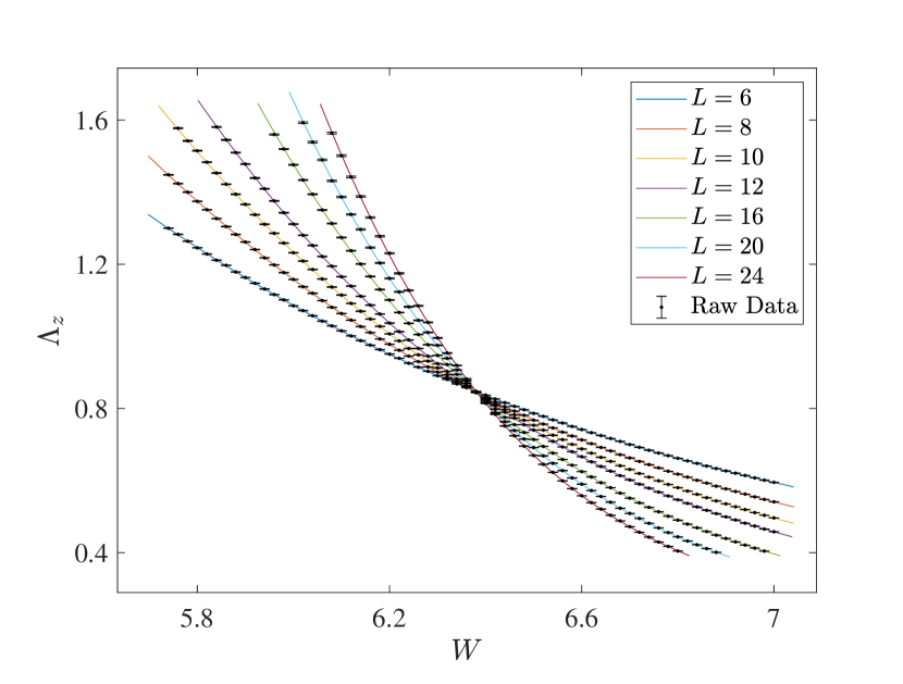
(a) $E=0$

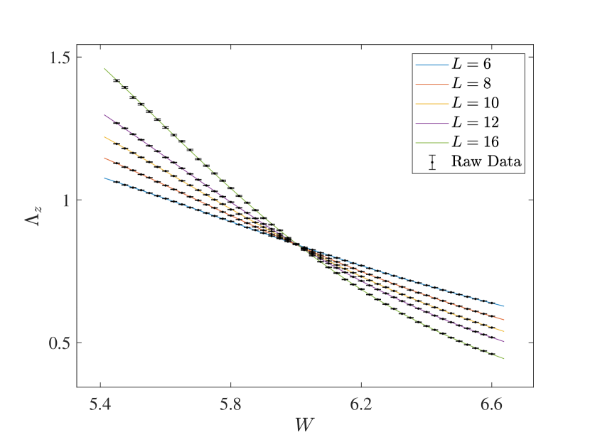
(b) $E={\rm i}$

Figure 4: Polynomial fitting of $\Lambda_{z}$ at (a) $E=0$ and (b) $E={\rm i}$ with $W_{r}=W_{i}=W$ for Anderson model. The black points with error bar are the raw data of $\Lambda_{z}$ and lines with different colors are the polynomial fitting results with expansion order ($m_{1}$, $n_{1}$, $m_{2}$, $n_{2}$)=(3,3,0,1).

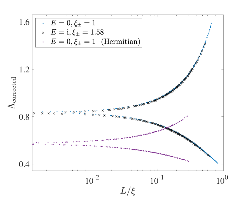
Figure 5: The data in Fig. 4 after subtraction of correction [see Eq. (85)] collapse into one curve according to scaling function Eq. (86). Here we set $\xi_{\pm}=1$ for $E=0$ and $\xi_{\pm}=1.58$ for $E={\rm i}$. The data of the Hermitian case at $E=0$ are also shown for the comparison.

In this subsection, we first compare critical properties of the Anderson transition at different energies in the complex plane. Eigenvalues of the NH systems are generally complex numbers and the eigenvalues of the NH Anderson model are distributed around $E=0$ in the Euler plane. In the Hermitian Anderson model, the Anderson transition for different energies appears at different critical disorder strength with the same critical exponent. A natural question arises in the NH Anderson model, asking whether the critical behaviors of the Anderson transition at different $E$ in the complex plane are the same or not. To answer this question, we calculate the localization length at $E=0$ and $E={\rm i}$, while changing the disorder strength $W$ along the symmetric line in the $W_{i}$-$W_{r}$ plane; $W_{r}=W_{i}=W$.

The localization length is calculated at $E=0$ with $L_{z}=10^{7}$ for $L=6,8,10,12,16$, $L_{z}=6\times 10^{6}$ for $L=20,24$; Fig. 4(a), and at $E={\rm i}$ with $L_{z}=10^{7}$ for $L=6,8,10,12$, $L_{z}=2\times 10^{6}$ for $L=16$; Fig. 4(b). Since there are no eigenstates at $E={\rm i}$ at $W=0$, the system at $E={\rm i}$ first undergoes a localization-delocalization transition at smaller critical disorder strength and then undergoes another delocalization-localization transition at larger critical disorder strength ($W_{c}\approx 6.02$). The two-steps transition at $E={\rm i}$ is similar to a reentrant phenomenon observed in Hermitian Anderson model near band edges[109, 85]. The density of states at $E={\rm i}$ is always finite around these two transition points. It is also finite at the Anderson transition at $E=0$ ($W_{c}\approx 6.39$). Let us compare the critical behaviors of $E=0$ at $W_{c}\approx 6.39$ with those of $E={\rm i}$ at $W_{c}\approx 6.02$.

The polynomial fitting method is used for the purpose of extracting critical quantities; Table 1. The critical disorder strength at $E=0$ is larger than those at $E={\rm i}$; delocalized states at the center of the complex plane is more robust than the states otherwise. The critical exponent $\nu\approx 1.19$, critical normalized localization length $\Lambda_{c}\approx 0.83$, and the least irrelevant scaling variable $y\approx 2.5$ are all consistent with each other between these two transition points. The coincidence suggests that the Anderson transition at different energies in the complex energy plane shares the same critical behaviors. $\nu$ and $\Lambda_{c}$ at these two points are distinct from those values of the 3D orthogonal class in the Hermitian case; $\nu\approx 1.57$ and $\Lambda_{c}\approx 0.58$ [73].

In order to determine a universal scaling function form of $\Lambda$ at the NH Anderson transition point, we subtract $\Lambda$ by the finite-size correction due to the irrelevant scaling variable,

$$\Lambda_{\rm corrected}\equiv\Lambda-\big{[}F(\phi_{1},\phi_{2})-F(\phi_{1},0)\big{]}.$$ (85)

According to Sec. II.2, the corrected $\Lambda$ must be given by a universal single-parameter scaling function near the transition point,

$$\Lambda_{\rm corrected}=f_{\pm}\Big{(}\frac{L}{\xi}\Big{)},$$ (86)

where $\xi\equiv\xi_{\pm}|u_{1}(\omega)|^{-\nu}$. Here $\xi_{\pm}$ depends on non-universal quantities in the polynomial fitting analysis, such as $a_{1,1}$, and they generally take different values at different single-particle energies and system parameters. However, $\xi_{+}/\xi_{-}$ would take a universal value [110]. Fig. 5 shows that with a proper choice of $\xi_{\pm}$, all the data points for $E=0$ and those for $E={\rm i}$ near the respective transition points fall into a single curve, demonstrating the validity of the universal single-parameter scaling function form for the corrected $\Lambda$. The single-parameter scaling function around the NH Anderson transition point is clearly distinct from that around the Hermitian Anderson transition point (Fig. 5). This unambiguously shows that the Anderson transition in the NH system belongs to a new universality class [56].

III.2 critical behaviors of the Anderson transition in the phase diagram at $E=0$ (NH Anderson model)

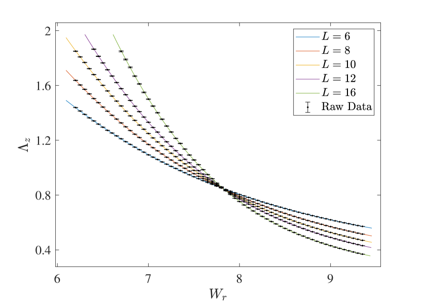
(a) $W_{i}=5$, (3,3,0,1)

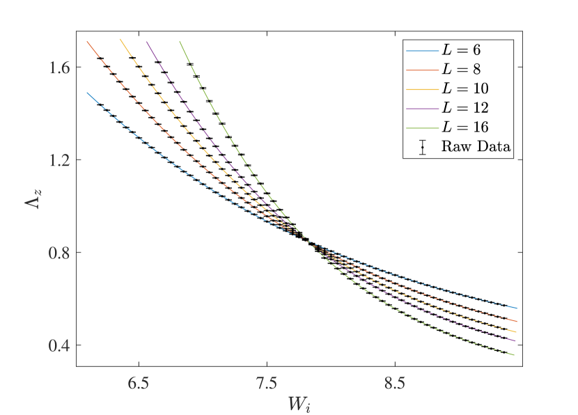
(b) $W_{r}=5$, (3,3,0,1)

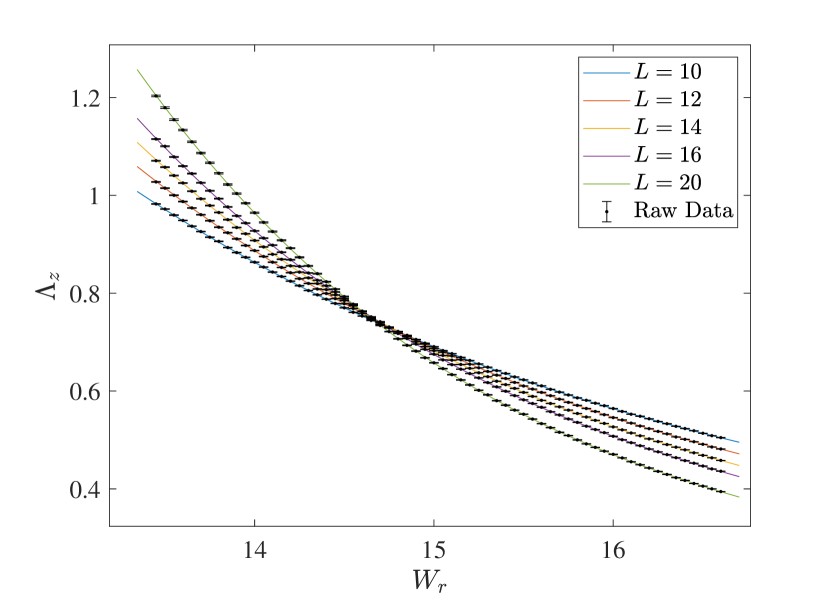
(c) $W_{i}=0.1$, (3,3,1,1)

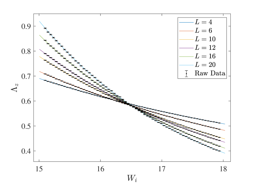
(d) $W_{r}=0$, (2,3,0,1)

Figure 6: Polynomial fitting for $\Lambda_{z}$ at $E=0$ with fixed $W_{r}$ or $W_{i}$ for the NH Anderson model. The black points with error bar are the raw data of $\Lambda_{z}$ and lines with different colors are the polynomial fitting results with expansion order ($m_{1}$, $n_{1}$, $m_{2}$, $n_{2}$). The expansion order ($m_{1}$, $n_{1}$, $m_{2}$, $n_{2}$) are shown in the brackets for each figure.

In this subsection, we compare critical properties of the Anderson transition at different system parameters of the same energy $E=0$. The localization length is calculated as a function of $W_{r}$ for fixed $W_{i}=5$; Fig. 6(a) or as a function of $W_{i}$ for fixed $W_{r}=5$; Fig. 6(b), where $L_{z}=10^{7}$ for $L=6,8,10,12$ and $L_{z}=3\times 10^{6}$ for $L=16$. The polynomial fitting results are summarized in the Table 1. In the Table, the critical exponent $\nu\approx 1.19$, the critical length $\Lambda_{c}\approx 0.83$, the least irrelevant scaling dimension and the critical disorder are consistent with each other for the fixed $W_{i}=5$ case and for the fixed $W_{r}=5$ case. Besides, the critical exponent and the critical length for these two transition points are consistent with those transition points at $E=0$ and $E={\rm i}$ along $W_{r}=W_{i}=W$. These comprehensive analyses conclude that the critical exponent for the Anderson transition in the NH Anderson model is

$$\nu=1.192[1.185,1.198].$$ (87)

The localization length at $E=0$ is also calculated as a function of $W_{i}$ for the fixed $W_{r}=0$ with $L_{z}=10^{7}$ for $L=4,6,10,12,16$, and $L_{z}=5\times 10^{6}$ for $L=20$; Fig. 6(d). Polynomial fitting results are shown in Table 1. As expected from the symmetry argument above, the critical exponent $\nu\approx 1.57$, the critical length $\Lambda_{c}\approx 0.58$ and and the critical disorder $W_{c}\approx 16.5$ coincide with those values in the Hermitian limit ($W_{i}=0$).

III.3 critical behaviors of the Anderson transition at $W_{r}=0$ and $E\neq 0$ (NH Anderson model)

The symmetric nature of the phase diagram and critical properties with respect to the exchange of $W_{r}$ and $W_{i}$ is absent at $E\neq 0$. Thereby, the critical point along the axis of $W_{r}=0$ must belong to the same universality class as the NH Anderson model. To confirm this, we calculate the localization length at $W_{r}=0$ and $E=2$ with $L_{z}=10^{7}$ for $L=8,10,12,16$ and with $L_{z}=6\times 10^{6}$ for $L=20$; Fig. 7. Polynomial fitting results are summarized in the Table 1. The critical disorder strength ($W_{c}\approx 11.1$) is clearly different from the value in the Hermitian limit ($W_{c}\approx 16.5$), demonstrating the asymmetry of the phase diagram at $E=2$. Both the critical exponent $\nu\approx 1.20$ and the critical length $\Lambda_{c}\approx 0.83$ are consistent with those values from $E=0$ and $E={\rm i}$ along $W_{r}=W_{i}=W$ and from $E=0$ along $W_{r(i)}=5$. The result reinforces the conclusion of Eq. (87).

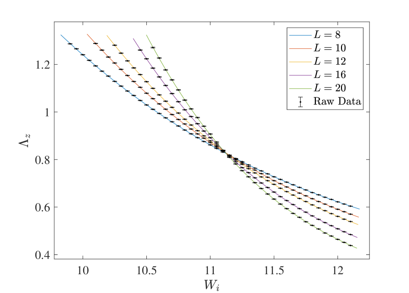
Figure 7: Polynomial fitting of $\Lambda_{z}$ at $E=2$ and $W_{r}=0$ for the NH Anderson model. The black points with error bar are the raw data of $\Lambda_{z}$ and lines with different colors are the polynomial fitting results with expansion order ($m_{1},n_{1},m_{2},n_{2}$)=(2,3,0,1).

III.4 RG flows at $E=0$ and at $E\neq 0$ and NH-H crossover phenomena (NH Anderson model)

In this subsection, we postulate an RG flow diagram in the $W_{r}$-$W_{i}$ plane at $E=0$ and at $E\neq 0$, based on the critical properties summarized in Sec. III.2 and Sec. III.3; Fig. 1(b, c). The RG flow diagram at $E=0$ has a saddle-point fixed point (FP3) with only one relevant scaling variable and two unstable fixed points (FP1 and FP2) with two relevant scaling variables. The FP3 determines the critical properties of delocalization–localization transition in the NH systems. When a simulated lattice model goes across the phase transition line, any dimensionless physical quantity is given by the universal function of the relevant scaling variable around FP3 and other irrelevant scaling variables. One of the irrelevant scaling variables is shown explicitly in the RG flow diagram in the $W_{r}$-$W_{i}$ plane.

The FP1 (FP2) controls the criticality in the Hermitian limit. When the lattice model crosses the transition line with either $W_{r}=0$ or $W_{i}=0$ at $E=0$, one of the two relevant scaling variables around FP1 (FP2) can be always set to zero. This is because the renormalization must respect the symmetry of the system and therefore it does not change a Hermitian system into a NH system. As a result, the quantity can be given by the universal function of only the other of the two relevant variables around FP1 (FP2); the Hermitian criticality. In the RG flow diagram at $E\neq 0$, FP1 disappears in the $W_{r}$-$W_{i}$ plane and all the critical properties except for those along the axis of $W_{i}=0$ are controlled by FP3; Fig. 1(c).

When the model undergoes the transition near FP2, the critical properties might exhibit a crossover phenomenon from the Hermitian case to the NH case. To study this crossover phenomenon, we calculate the localization length at $E=0$ for fixed $W_{i}=0.1$ with $L_{z}=10^{7}$ for $L=10,12,14,16$ and $L_{z}=6\times 10^{6}$ for $L=20$; Fig. 6(c). The fitting results are summarized in Table 1. According to the fitting results, the scaling dimension of the least irrelevant scaling variable is quite small, indicating the importance of the irrelevant scaling variables. In fact, the large correction by the irrelevant scaling variables results in a bad intersection of $\Lambda_{z}$ in the data. The critical exponent in the fitting results is consistent neither with that for the Hermitian case nor with that for the NH case. To capture the correct critical properties in this crossover regime, we believe it necessary either to include the non-linear $\phi_{2}$-dependence of $F$ ($n_{2}>1$) together with the non-linear $w$-dependence of $u_{2}(w)$ ($m_{2}>1$) or to fit only the larger system size data.

III.5 conductance (NH Anderson model)

As in the Hermitian case [91, 111], the conductance is a convenient physical quantity that can characterize the critical property of the Anderson transition in the NH systems. As shown in the previous section, the conductance in the NH systems is not bounded by the total number of the transmission channels in the two-terminal geometry. The transmission amplitude can be arbitrarily amplified by the on-site NH disorder potentials in the NH systems.

Fig. 8 shows distributions of the conductance in the NH Anderson models, where the conductance is calculated in terms of Eqs. (52), (29), and (49) with the cubic geometry $L_{x}=L_{y}=L_{z}=L$ for $10^{6}$ samples of different disorder realizations. We have changed the frequency of the $QR$ decomposition in the transfer matrix calculation, and checked the results in Fig. 8 are robust against the change. The three figures in Fig. 8 show that the distribution of the conductance is not Gaussian irrespective of whether the system is in the delocalized phase or in the localized phase or at the critical point. The conductance distribution always contains small fractions of huge conductance values. The very large conductance values come from ‘rare-event’ states, in which the transmission is strongly amplified by the NH disorders. To carry out the FSS analysis for such conductance data, we take a geometric mean of the conductance; $\langle\ln g\rangle$. The plot of the geometric average of the conductance and its fit to polynomial functions are shown in Appendix.

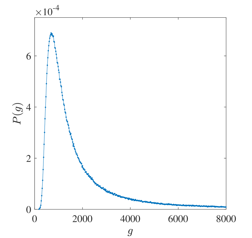
(a) $W=1$, metal phase

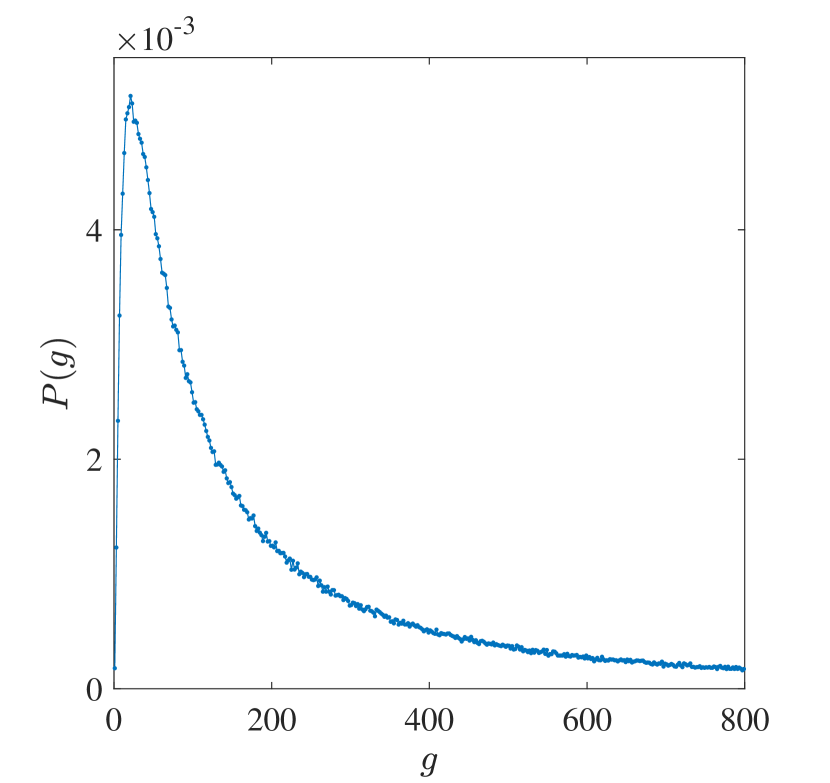
(b) $W=6.386$, near critical point

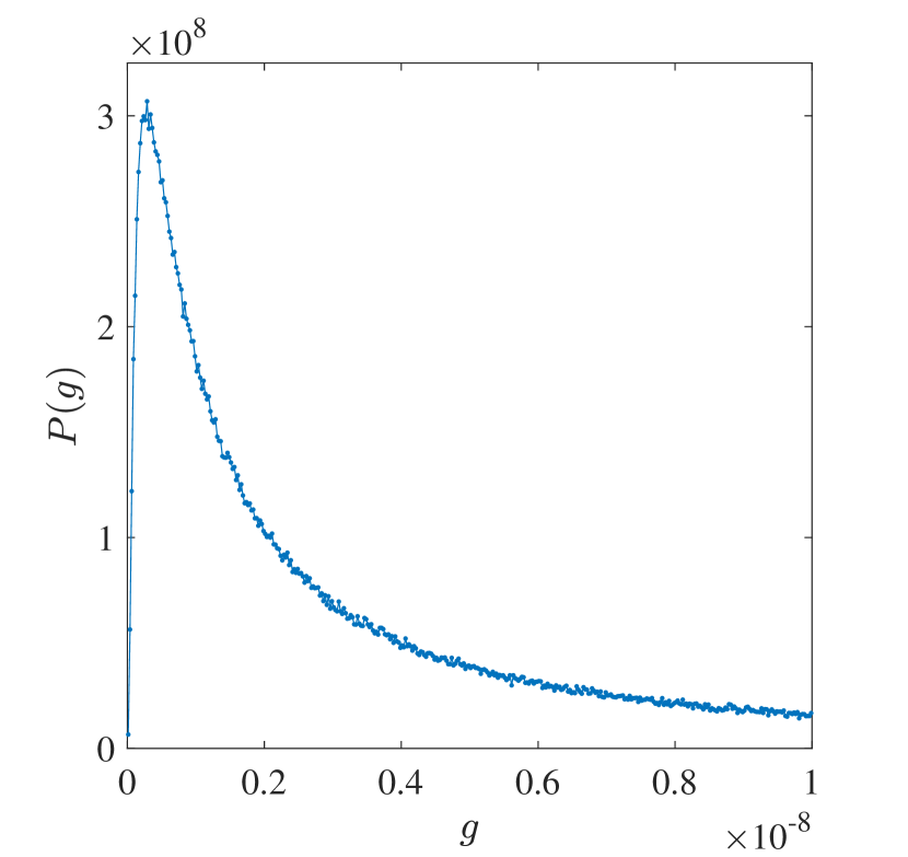
(c) $W=14$, insulator phase

Figure 8: Conductance distribution $P(g)$ of the Anderson model with non-Hermitian disorder. $10^{6}$ samples are calculated for $L=12$ at $E=0$ and $W_{r}=W_{i}=W$. (a) $W=1$: metallic phase, (b) $W=6.386$: critical point, and (c) $W=14$: localized phase. The distribution has a long tail in a region of very large conductance value. The horizontal axis is an arbitrary unit. Only $93\%,83\%,68\%$ of the whole data points are shown in (a,b,c), respectively.

IV non-Hermitian class A models

In this section, we give an accurate characterization of the critical properties of the Anderson transition in the two NH class A models; NH U(1) and Peierls models. From the symmetry argument above, the $E=0$ phase diagrams of these two models must also be symmetric with respect to the exchange of $W_{r}$ and $W_{i}$. At $E=0$, both the axis of $W_{r}=0$ and the axis of $W_{i}=0$ belong to the Hermitian class A. We expect that an effect of the irrelevant scaling variable can be minimized along the symmetry line of $W_{r}=W_{i}$. Based on this anticipation, we focus our study on the Anderson transition in the two NH class A models along the axis of $W_{r}=W_{i}=W$, setting $E=0$.

IV.1 NH U(1) model at $E=0$

In this subsection, we first clarify the critical property of the Anderson transition in the NH U(1) model. The localization length has been calculated with $L_{z}=10^{7}$ for $L=8,10,12,16$, and with $L_{z}=6\times 10^{6}$ for $L=20,24$. For the purpose of the transfer matrix calculations, it is convenient to perform a gauge transformation of the original Hamiltonian so as to eliminate all the random U(1) phase factors appearing in hopping elements in the $z$-direction. Obviously, the transformation does not affect the values of the Lyapunov exponents [65]. The normalized localization length near its scale invariant point is shown in Fig. 9. The polynomial fitting result is summarized in Table 1. The critical exponent is evaluated from the fitting as

$$\nu=1.003[0.985,1.018],$$ (88)

together with $\Lambda_{c}\approx 0.598$. These two universal quantities are clearly distinct from $\nu\approx 1.44$ and $\Lambda_{c}\approx 0.55$ for the Hermitian U(1) model [65]. They are also different from the $\nu\approx 1.19$ and $\Lambda_{c}\approx 0.83$ for the NH Anderson model (NH class AI^†). As was pointed out in Ref. 56, $W_{c}\approx 7.3$ for the NH U(1) model is significantly larger than $W_{c}$ for the NH Anderson model ($W_{c}\approx 6.4$), in spite of the fact that the NH U(1) model has more random variables in its off-diagonal matrix elements than the NH Anderson model. This means that the delocalization-localization transition in the NH system is also of the quantum interference origin.

The two-terminal conductance $g$ is also calculated in the NH U(1) model along the axis of $W_{r}=W_{i}=W$ at $E=0$. A plot of the geometric average of the conductance and the details of the polynomial fitting are given in the Appendix.

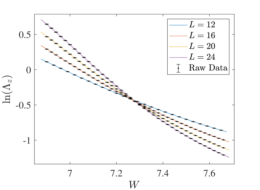
Figure 9: Polynomial fitting of $\ln(\Lambda_{z})$ at $E=0$ with $W_{r}=W_{i}=W$ for the NH U(1) model. The black points with error bar are the raw data of $\ln(\Lambda_{z})$ and lines with different colors are the polynomial fitting results with expansion order ($m_{1}$, $n_{1}$, $m_{2}$, $n_{2}$)=(3,3,0,1).

IV.2 NH Peierls model at $E=0$

In this subsection, we clarify the critical property of the Anderson transition in the NH Peierls model with the magnetic flux $2\pi\Phi=\pi/2$. The localization length is calculated with $L_{z}=10^{7}$ for $L=8,10,12,16,20$. The normalized localization length near its scaling invariant point is shown in Fig. 10. The polynomial fitting results are summarized in Table 1. For our choice of the data range, we need to take $n_{1}=4$ to obtain a sufficiently large goodness of fit in the polynomial fitting. The large $n_{1}$ represents a non-linear $\phi_{1}$-dependence of $F$ around the critical point ($\phi_{1}=0$). The fittings with the system size $L=10\sim 20$ and the expansion order ($m_{1}$, $n_{1}$, $m_{2}$, $n_{2}$)=(2,4,0,1) or (3,4,0,1) give stable fitting results with the critical exponent $\nu=1.02\pm 0.01$. This value is quite close to the critical exponent in the NH U(1) model, supporting Eq. (88) as the critical exponent in the 3D NH class A systems. Note that the uniform magnetic flux $\Phi$ introduces a geometric anisotropy in the Peierls model. As a result, the critical normalized length $\Lambda_{c}$ in the NH Peierls model is different from that in the NH U(1) model (Table 1), although the nearest-neighbor hopping amplitudes in these two cubic-lattice models are all same in the three directions.

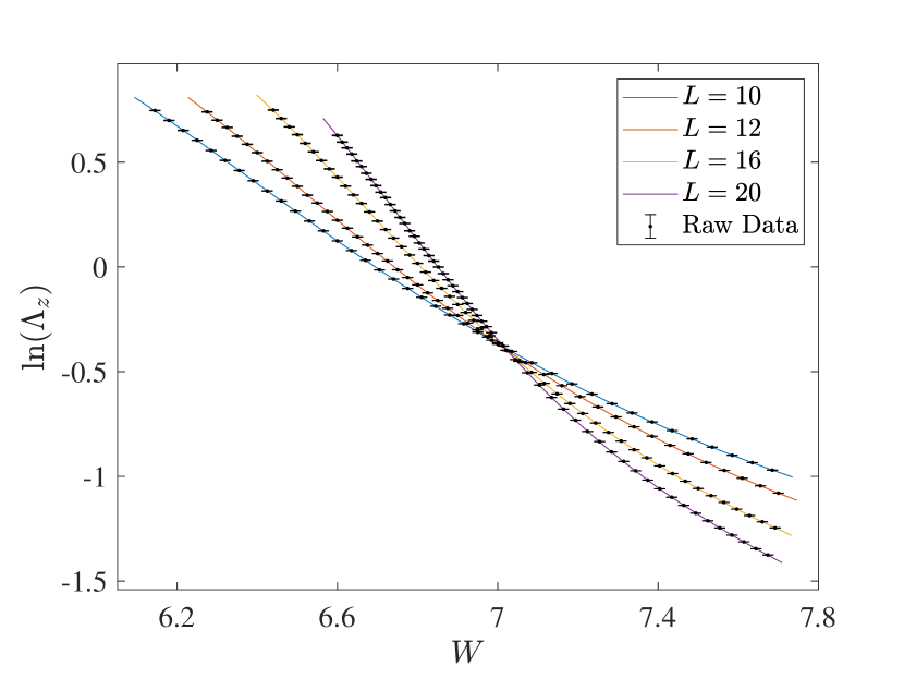
Figure 10: Polynomial fitting of $\ln(\Lambda_{z})$ at $E=0$ and $W_{r}=W_{i}=W$ for the NH Peierls model with the magnetic flux $\Phi=1/4$. The black points with error bar are the raw data of $\ln(\Lambda_{z})$ and lines with different colors are the polynomial fitting results with expansion order ($m_{1},n_{1},m_{2},n_{2}$)=(3,4,0,1).

V revisiting the level statistics analysis

In this section, we compare the critical exponents evaluated by the localization length with the previous evaluation by the level statistics in the NH Anderson and U(1) models [56]. The level statistics analysis [59, 60, 61] introduces a finite energy window over which the dimensionless quantity $\Gamma$ is averaged. When applying a linear fitting with respect to $w\equiv(W-W_{c})/W_{c}$, $\Gamma(W,L)=\Gamma_{c}+awL^{1/\nu}$ with $(m_{1},n_{1},m_{2},n_{2})=(1,1,0,0)$ in Eq. (69), the finite width of the energy window does not cause any influence on the estimate of the critical exponent $\nu$; $a$ and $W_{c}$ are averaged over the energy window, while $\Gamma_{c}$ and $\nu$ take the same universal values for any states within the window. When applying a non-linear fitting of $\Gamma$ with resepct to $w$, the analysis needs to assume that all the fitting parameters in the universal function $F$ in Eq. (69) have no variations within the energy window. As explained in Sec. II.2, however, these fitting parameters include not only the universal critical exponent but also non-universal critical quantities, such as critical disorder strength $W_{c}$, and the scaling dimensions of the irrelevant scaling variables $y$. Generally, two cases with different energies do not share the same non-universal critical quantities. They are continuous functions of the energy. Thus, the energy window for the level statistics must be narrow enough so that all the states inside the window share almost the same values of these fitting parameters. Otherwise, the variations of the non-universal fitting parameters cause additional systematic errors in the estimate of the universal critical exponent.

With the above consideration in mind, we first discuss the critical exponent of the 3D class A models. The value obtained in this paper is consistent with the critical exponent of the NH U(1) model obtained by the level statistics analysis [56]; $\nu\approx 1.09$ by the level statistics for 10% eigenvalues around $E=0$, and $\nu\approx 1.01$ for 5% eigenvalues around $E=0$. Namely, the critical exponent of the 3D class A models in this paper is closer to the value for the 5% energy window than to the value for the 10% energy window. This tendency suggests that the level statistics analysis for the narrower energy window are relatively free from the effects of finite variations of the non-universal critical quantities.

On the one hand, the critical exponent of the 3D NH Anderson model (NH class AI^†) obtained in this paper is at variance with the critical exponent obtained by the level statistics analysis in Ref. 56; $\nu\approx 0.99$ by the level statistics for 10% eigenvalues around $E=0$, and $\nu\approx 0.95$ for 5% eigenvalues around $E=0$. We regard that the discrepancy comes from an interplay between the finite-energy window issue and a strong asymmetry in a universal function for a level spacing ratio [112, 54, 113] around the Anderson transition point. The level spacing ratio $r$ exhibits limiting values [56, 113] as a function of the disorder strength in the NH Anderson model; $\langle r\rangle_{\rm loc}=2/3$ in the localized phase and $\langle r\rangle_{\rm deloc}\approx 0.72$ in the delocalized phase. It turns out that an intersection of curves of $\langle r\rangle$ for different system sizes, $\langle r\rangle_{\rm critical}=0.716$, is very close to one of the two limiting values, $\langle r\rangle_{\rm deloc}\approx 0.72$. This indicates that the universal function for the level spacing ratio happens to be quite asymmetric around the transition point in the NH Anderson model. When fitting such an asymmetric function by the polynomial in $w$, the polynomial function must have a strong nonlinear $w$-dependence. Thus, the finite-energy window issue together with this intrinsic strong non-linearity in the universal function for the level spacing ratio causes large systematic errors in the NH Anderson model. In other words, a valid data range of polynomial fitting analysis with the smaller $n_{1}$ and $m_{1}$ becomes very small in the side of the delocalized phase and the choice of the data points in the previous study is not narrow enough in the NH Anderson model.

In summary, the argument so far concludes the critical exponent $\nu=1.19\pm 0.01$ in the Anderson transition in the NH symmetry class AI^†, and $\nu=1.00\pm 0.04$ in the Anderson transition in the NH symmetry class A. In spite of the correction of the critical exponent in the NH class AI^†, our previous conclusion in the level statistics analysis remains unchanged. Namely, 3D NH Anderson transition in classes AI^† and in class A show critical behaviors different from their Hermitian counterparts, hence belong to new universality classes.

VI Summary

Model	class	$H$	$M$	Lyapunov	$S$	unitarity	$g$
H AM	AI	$H=H^{\mathrm{T}}=H^{*}$	$\sigma_{y}M^{\mathrm{T}}\sigma_{y}=M^{-1}$	$\gamma_{i}=\gamma_{i}^{\prime}$	$S=S^{\mathrm{T}}$	$S^{\dagger}S=I$	$g_{L}=g_{R}$
H U	A	$H=H^{\dagger}$	$\sigma_{y}M^{\dagger}\sigma_{y}=M^{-1}$	$\gamma_{i}=\gamma_{i}^{\prime}$	–	$S^{\dagger}S=I$	$g_{L}(\pm\{\phi\})=g_{R}(\pm\{\phi\})$
NH AM	NH AI†	$H=H^{\mathrm{T}}$	$\sigma_{y}M^{\mathrm{T}}\sigma_{y}=M^{-1}$	$\gamma_{i}=\gamma_{i}^{\prime}$	$S=S^{\mathrm{T}}$	$S^{\dagger}(H)S(H^{\dagger})=I$	$g_{L}=g_{R}$
NH U	NH A	–	–	$\langle\gamma_{i}\rangle=\langle\gamma_{i}^{\prime}\rangle$	–	$S^{\dagger}(H)S(H^{\dagger})=I$	$g_{L}(\{\phi\})=g_{R}(-\{\phi\})$
p-H		$\eta H\eta^{-1}=H^{\dagger}$	$\eta\sigma_{y}M^{\mathrm{\dagger}}(E)\sigma_{y}\eta^{-1}=M^{-1}(E^{*})$	$\gamma_{i}(E)=\gamma_{i}^{\prime}(E^{*})$		$S^{\dagger}(E)\eta S(E^{*})=\eta$	$g_{L}=g_{R}$

Table 2: Summary of symmetry relations of Lyapunov exponents (‘Lyapunov’), the $S$ matrix ($S$) and two-terminal conductances ($g$) in Sec. II. The columns of $H$ and $M$ specify the symmetries of Hamiltonian and transfer matrix in the Hermitian Anderson model (H AM), non-Hermitian Anderson model (NH AM), Hermitian U(1)/Peierls model (H U) and non-Hermitian U(1)/Peierls model (NH U). ‘$\gamma_{i}=\gamma^{\prime}_{i}$’ in the column of ‘Lyapunov’ stands for a $\pm$ symmetry of the Lyapunov exponents: the Lyapunov exponents are ordered such that $\gamma_{n}>\cdots\gamma_{2}>\gamma_{1}>0>-\gamma_{1}^{\prime}>-\gamma_{2}^{\prime}\cdots>-\gamma_{n}^{\prime}$, $2n=2L_{x}L_{y}$ being the dimensions of the transfer matrix. In the non-Hermitian case, a Hermitian conjugate of a $S$ matrix for $H$ is an inverse of a $S$ matrix of $H^{\dagger}$; $S^{\dagger}(H)=S^{-1}(H^{\dagger})$. For the NH U(1)/Peierls models, the leftward conductance with a position dependent magnetic flux $\{\phi\}$ is identical to the rightward conductance with $-\{\phi\}$; $g_{L}(\{\phi\})=g_{R}(-\{\phi\})$. For the Hermitian U(1)/Peierls models, the unitarity of the scattering matrix gives an equivalence between the leftward conductance and rightward conductance; $g_{L}(\{\phi\})=g_{R}(\{\phi\})=g_{L}(-\{\phi\})=g_{R}(-\{\phi\})$. ‘p-H’ indicates non-Hermitian systems with the pseudo-Hermiticity in Sec. II.1.3. $\eta$ is a Hermitian and unitary matrix.

In this paper, we presented transfer matrix analyses of the Anderson transition in the three NH systems with on-site complex-valued random potentials that belong to the class-AI^† (NH Anderson model) and class-A (NH U(1) and NH Peierls models), respectively. We first provided an argument with solid numerical evidence that supports the validity of the transfer matrix analyses of the localization length and two-terminal conductance in NH systems. We then clarified the presence or absence of the reciprocal symmetries of the Lyapunov exponent and the conductance in the three NH models. The relations are summarized in Table 2. We note that other relations in non-reciprocal non-Hermitian systems are found in [114].

On the basis of the above knowledge, we evaluated the critical exponents at different single-particle energies and different system parameters of the NH Anderson model as well as of the NH U(1) and NH Peierls models. The results conclude that the critical exponent of the NH class-AI^† is $\nu=1.19\pm 0.01$ and the critical exponent of the NH class-A is $\nu=1.00\pm 0.04$, indicating a strong linkage between the universality class of the Anderson transition and symmetry classification in the NH systems. From the critical properties at different system parameters of the NH Anderson model, we draw a phase diagram in a two-dimensional plane subtended by the disorder strength of the real part of the on-site random potential ($W_{r}$) and that of the imaginary part ($W_{i}$). We showed that at the zero single-particle energy ($E=0$), the phase diagram as well as the critical properties become completely symmetric with respect to an exchange between $W_{r}$ and $W_{i}$. We further proved that the symmetric structure at the zero single-particle energy is a generic feature in any NH bipartite-lattice models with the on-site NH random potentials. We also demonstrated numerically that a distribution of the two-terminal conductance is not Gaussian and the distribution contains small numbers of huge conductance, which come from rare events of strong amplifications of the transmission by the NH disorders. By analyzing the geometric mean of the conductance, we show that the critical properties of the conductance in the NH Anderson and NH U(1) models also give critical exponents, which are consistent with those critical exponents obtained by the localization length. We note that Wegner’s relation[115], which relates the conductivity critical exponent $s$ and the localization critical exponent $\nu$ as $s=(d-2)\nu=\nu$, remains to be checked in NH systems.

In conclusion, an experimental verification of the new universality classes in the NH systems may be possible in disordered optical systems [116, 117, 118, 119, 120] and acoustic systems [121, 122, 123], which usually fall into the 3D NH class AI^†. The energy loss and gain in the optical systems make it difficult to verify the Anderson transition in the Hermitian systems. On the other hand, disordered media with gain and loss are ideal platforms for an experimental verification of the Anderson transition in NH systems [52, 124]. An experimental realization of the NH class A model in the disordered optical systems seems to be non-trivial, and we leave it for an important future problem.

*

Appendix A Two-terminal conductance and its finite-size scaling analysis

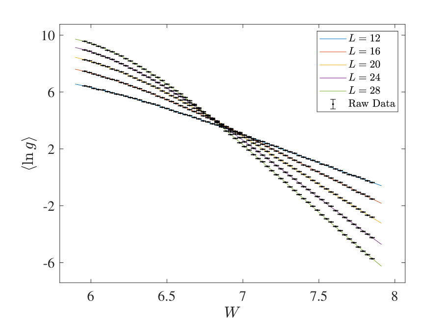
Figure 11: Polynomial fitting for $\langle\ln g\rangle$ at $E=0$ with $W_{r}=W_{i}=W$ for the NH Anderson model with periodic boundary condition in the $x$ and $y$ directions. The black points with error bar are the raw data of $\langle\ln g\rangle$ and lines with different colors are the polynomial fitting results with the expansion order $(m_{1},n_{1},m_{2},n_{2})=(2,3,0,1)$. $\langle\ln g\rangle$ are averaged over $10^{4}$ samples. Note also that the reciprocal relation of the conductance is verified numerically in each sample.

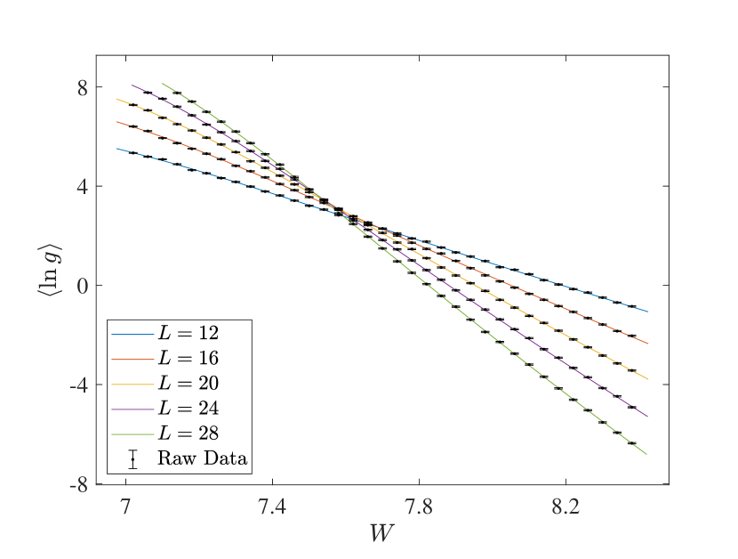
(a) PBC, (3,3,0,1)

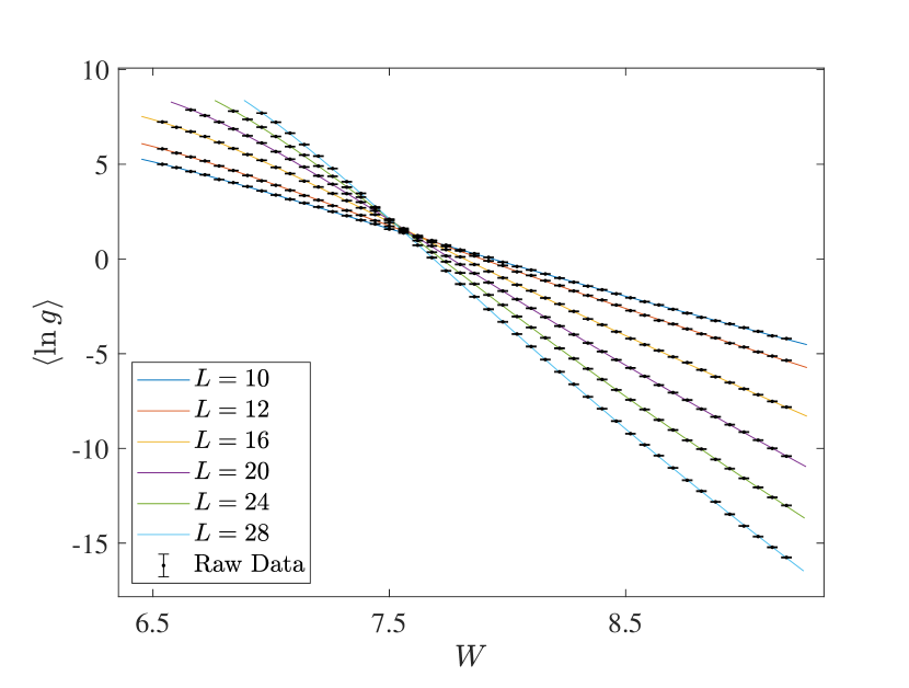
(b) OBC, (3,3,0,1)

Figure 12: Polynomial fitting for $\langle\ln g\rangle$ at $E=0$ with $W_{r}=W_{i}=W$ for the NH U(1) model with the (a) periodic boundary condition (PBC) and (b) open boundary condition (OBC). The black points with error bar are the raw data of $\langle\ln g\rangle$ and lines with different colors are the polynomial fitting results with expansion order $(m_{1},n_{1},m_{2},n_{2})$. The expansion order ($m_{1}$, $n_{1}$, $m_{2}$, $n_{2}$) are shown in the brackets for each figure. $\langle\ln g\rangle$ are averaged over $10^{4}$ samples.

Table 3: Polynomial fitting results for the logarithm of the conductance $\langle\ln g\rangle$ around the Anderson transition points in the NH Anderson and U(1) models at $W_{r}=W_{i}=W$ and $E=0$. The goodness of fit (GOF), critical disorder $W_{c}$, critical exponent $\nu$, the scaling dimension of the least irrelevant scaling variable $-y$ are shown for various system sizes and for different expansion orders of the polynomial: $(m_{1},n_{1},m_{2},n_{2})$. The square bracket stands for the 95% confidence interval.

NH Anderson model, with the PBC
$L$	$m_{1}$	$n_{1}$	$m_{2}$	$n_{2}$	GOF	$W_{c}$	$\nu$	$y$
12-28	2	3	0	1	0.20	6.415[6.387, 6.523]	1.276[0.998, 1.454]	0.06[0.03, 0.32]
12-28	3	3	0	1	0.23	6.415[6.385, 6.513]	1.288[1.006, 1.524]	0.06[0.03, 0.30]
16-28	2	3	0	1	0.20	6.415[6.387, 6.520]	1.276[1.002, 1.457]	0.06[0.03, 0.31]
16-28	3	3	0	1	0.23	6.415[6.385, 6.522]	1.288[1.006, 1.520]	0.06[0.03, 0.31]
NH U(1) model, with the PBC
$L$	$m_{1}$	$n_{1}$	$m_{2}$	$n_{2}$	GOF	$W_{c}$	$\nu$	$y$
12-28	3	3	0	1	0.10	7.338[7.323, 7.435]	1.142[0.861, 1.349]	0.044[0.024, 0.639]
16-28	3	3	0	1	0.10	7.329[7.295, 7.362]	1.150[0.859, 1.479]	0.046[0.039, 0.091]
NH U(1) model, with the OBC
$L$	$m_{1}$	$n_{1}$	$m_{2}$	$n_{2}$	GOF	$W_{c}$	$\nu$	$y$
10-28	3	3	0	1	0.24	7.391[7.379, 7.444]	1.069[0.961, 1.130]	0.12[0.07, 0.55]
12-28	3	3	0	1	0.12	7.397[7.381, 7.454]	1.075[0.950, 1.162]	0.15[0.08, 0.70]

In this appendix, we describe behaviours of the two-terminal conductance as a function of disorder strength and the FSS analyses of the conductance for the NH Anderson and U(1) models.

Fig. 11 shows the logarithm of the conductance $g$ as a function of $W$ in the NH Anderson model at $W_{r}=W_{i}=W$ and $E=0$. Thereby, the conductance $g$ is calculated in terms of Eqs. (52,29,49) with the cubic geometry $L_{x}=L_{y}=L_{z}=L$ and periodic boundary condition (PBC) along the $x$ and $y$ direction. The logarithm of $g$ is averaged over $10^{4}$ samples of different disorder realizations. $\langle\ln g\rangle$ for different system size $L$ show an intersection near the critical disorder strength determined by the Lyapunov exponent analysis. Nonetheless, the intersection point of $\langle\ln g\rangle$ for different system sizes is not as obvious as in the Lyapunov exponent, even for larger system size ($L=16,20,24,28$); $\langle\ln g\rangle$ among larger system sizes tends to intersect at a smaller disorder strength.

The critical exponent is obtained from the polynomial fitting analysis (Table 3). The critical exponent evaluated from $\langle\ln g\rangle$ is slightly larger than the critical exponent determined by the Lyapunov exponent, while they are consistent with each other within the 95% confidence intervals. Note that the scaling dimension of the least irrelevant scaling variable is quite small in the polynomial fitting analysis of $\langle\ln g\rangle$, which results in a large error bar for $\nu$. The poor estimation of the critical property comes from the poor intersection of $\langle\ln g\rangle$. Two reasons could be responsible for the poor intersection; (i) a non-optimal choice of the contact between the Hermitian leads and the NH system and (ii) intrinsically large values of the conductance due to the non-Hermiticity.

Fig. 12 shows plots of the logarithm of the conductance as a function of $W$ in the NH U(1) model at $W_{r}=W_{i}=W$ and $E=0$ with the same conditions as above, except for the boundary condition along the $x$ and $y$ direction. The plot with the PBC is in Fig. 12(a) and the plot with the open boundary condition (OBC) is in Fig. 12(b). The polynomial fitting result is summarized in Table 3. As in the NH Anderson model, the critical disorder strength from the fitting is slightly larger than the critical disorder strength determined by the Lyapunov exponent and the intersection point shifts to a smaller value for larger system sizes. Nonetheless, the critical exponent is consistent with the critical exponent determined by the Lyapunov exponent within the 95% confidence interval. Note that the smaller value of $y$ from the fitting analysis indicates a strong finite-size correction, which leads to a large error bar of the critical exponent and the poor intersection. Note also that the intersection of the conductance with the OBC is better than that with the PBC. This phenomenon doesn’t occur for the NH Anderson model.

References

- Esaki et al. [2011] K. Esaki, M. Sato, K. Hasebe, and M. Kohmoto, Edge states and topological phases in non-hermitian systems, Phys. Rev. B 84, 205128 (2011).
- Lee [2016] T. E. Lee, Anomalous edge state in a non-hermitian lattice, Phys. Rev. Lett. 116, 133903 (2016).
- Leykam et al. [2017] D. Leykam, K. Y. Bliokh, C. Huang, Y. D. Chong, and F. Nori, Edge modes, degeneracies, and topological numbers in non-hermitian systems, Phys. Rev. Lett. 118, 040401 (2017).
- Kunst et al. [2018] F. K. Kunst, E. Edvardsson, J. C. Budich, and E. J. Bergholtz, Biorthogonal bulk-boundary correspondence in non-hermitian systems, Phys. Rev. Lett. 121, 026808 (2018).
- Martinez Alvarez et al. [2018] V. M. Martinez Alvarez, J. E. Barrios Vargas, and L. E. F. Foa Torres, Non-hermitian robust edge states in one dimension: Anomalous localization and eigenspace condensation at exceptional points, Phys. Rev. B 97, 121401 (2018).
- Yao and Wang [2018] S. Yao and Z. Wang, Edge states and topological invariants of non-hermitian systems, Phys. Rev. Lett. 121, 086803 (2018).
- Yao et al. [2018] S. Yao, F. Song, and Z. Wang, Non-hermitian chern bands, Phys. Rev. Lett. 121, 136802 (2018).
- Gong et al. [2018] Z. Gong, Y. Ashida, K. Kawabata, K. Takasan, S. Higashikawa, and M. Ueda, Topological phases of non-hermitian systems, Phys. Rev. X 8, 031079 (2018).
- Lieu [2018] S. Lieu, Topological phases in the non-hermitian su-schrieffer-heeger model, Phys. Rev. B 97, 045106 (2018).
- Yin et al. [2018] C. Yin, H. Jiang, L. Li, R. Lü, and S. Chen, Geometrical meaning of winding number and its characterization of topological phases in one-dimensional chiral non-hermitian systems, Phys. Rev. A 97, 052115 (2018).
- Yokomizo and Murakami [2019] K. Yokomizo and S. Murakami, Non-bloch band theory of non-hermitian systems, Phys. Rev. Lett. 123, 066404 (2019).
- Deng and Yi [2019] T.-S. Deng and W. Yi, Non-bloch topological invariants in a non-hermitian domain wall system, Phys. Rev. B 100, 035102 (2019).
- Song et al. [2019a] F. Song, S. Yao, and Z. Wang, Non-hermitian topological invariants in real space, Phys. Rev. Lett. 123, 246801 (2019a).
- Liu et al. [2019] T. Liu, Y.-R. Zhang, Q. Ai, Z. Gong, K. Kawabata, M. Ueda, and F. Nori, Second-order topological phases in non-hermitian systems, Phys. Rev. Lett. 122, 076801 (2019).
- Zhou and Lee [2019] H. Zhou and J. Y. Lee, Periodic table for topological bands with non-hermitian symmetries, Phys. Rev. B 99, 235112 (2019).
- Kawabata et al. [2019a] K. Kawabata, K. Shiozaki, M. Ueda, and M. Sato, Symmetry and topology in non-hermitian physics, Phys. Rev. X 9, 041015 (2019a).
- Kawabata et al. [2019b] K. Kawabata, S. Higashikawa, Z. Gong, Y. Ashida, and M. Ueda, Topological unification of time-reversal and particle-hole symmetries in non-hermitian physics, Nature Communications 10, 297 (2019b).
- Song et al. [2019b] F. Song, S. Yao, and Z. Wang, Non-hermitian skin effect and chiral damping in open quantum systems, Phys. Rev. Lett. 123, 170401 (2019b).
- Okuma and Sato [2019] N. Okuma and M. Sato, Topological phase transition driven by infinitesimal instability: Majorana fermions in non-hermitian spintronics, Phys. Rev. Lett. 123, 097701 (2019).
- Lee et al. [2019] C. H. Lee, L. Li, and J. Gong, Hybrid higher-order skin-topological modes in nonreciprocal systems, Phys. Rev. Lett. 123, 016805 (2019).
- Jiang et al. [2019] H. Jiang, L.-J. Lang, C. Yang, S.-L. Zhu, and S. Chen, Interplay of non-hermitian skin effects and anderson localization in nonreciprocal quasiperiodic lattices, Phys. Rev. B 100, 054301 (2019).
- Ezawa [2019] M. Ezawa, Braiding of majorana-like corner states in electric circuits and its non-hermitian generalization, Phys. Rev. B 100, 045407 (2019).
- Okuma et al. [2020] N. Okuma, K. Kawabata, K. Shiozaki, and M. Sato, Topological origin of non-hermitian skin effects, Phys. Rev. Lett. 124, 086801 (2020).
- Guo et al. [2009] A. Guo, G. J. Salamo, D. Duchesne, R. Morandotti, M. Volatier-Ravat, V. Aimez, G. A. Siviloglou, and D. N. Christodoulides, Observation of -symmetry breaking in complex optical potentials, Phys. Rev. Lett. 103, 093902 (2009).
- Rüter et al. [2010] C. E. Rüter, K. G. Makris, R. El-Ganainy, D. N. Christodoulides, M. Segev, and D. Kip, Observation of parityâtime symmetry in optics, Nature Physics 6, 192 (2010).
- Feng et al. [2011] L. Feng, M. Ayache, J. Huang, Y.-L. Xu, M.-H. Lu, Y.-F. Chen, Y. Fainman, and A. Scherer, Nonreciprocal light propagation in a silicon photonic circuit, Science 333, 729 (2011).
- Regensburger et al. [2012] A. Regensburger, C. Bersch, M.-A. Miri, G. Onishchukov, D. N. Christodoulides, and U. Peschel, Parity–time synthetic photonic lattices, Nature 488, 167 (2012).
- Zeuner et al. [2015] J. M. Zeuner, M. C. Rechtsman, Y. Plotnik, Y. Lumer, S. Nolte, M. S. Rudner, M. Segev, and A. Szameit, Observation of a topological transition in the bulk of a non-hermitian system, Phys. Rev. Lett. 115, 040402 (2015).
- Malzard et al. [2015] S. Malzard, C. Poli, and H. Schomerus, Topologically protected defect states in open photonic systems with non-hermitian charge-conjugation and parity-time symmetry, Phys. Rev. Lett. 115, 200402 (2015).
- Zhen et al. [2015] B. Zhen, C. W. Hsu, Y. Igarashi, L. Lu, I. Kaminer, A. Pick, S.-L. Chua, J. D. Joannopoulos, and M. Soljačić, Spawning rings of exceptional points out of dirac cones, Nature 525, 354 (2015).
- Weimann et al. [2017] S. Weimann, M. Kremer, Y. Plotnik, Y. Lumer, S. Nolte, K. G. Makris, M. Segev, M. C. Rechtsman, and A. Szameit, Topologically protected bound states in photonic parity-time-symmetric crystals, Nature Materials 16, 433 (2017).
- Xiao et al. [2017] L. Xiao, X. Zhan, Z. H. Bian, K. K. Wang, X. Zhang, X. P. Wang, J. Li, K. Mochizuki, D. Kim, N. Kawakami, W. Yi, H. Obuse, B. C. Sanders, and P. Xue, Observation of topological edge states in parityâtime-symmetric quantum walks, Nature Physics 13, 1117 (2017).
- Bahari et al. [2017] B. Bahari, A. Ndao, F. Vallini, A. El Amili, Y. Fainman, and B. Kanté, Nonreciprocal lasing in topological cavities of arbitrary geometries, Science 358, 636 (2017).
- Zhou et al. [2018] H. Zhou, C. Peng, Y. Yoon, C. W. Hsu, K. A. Nelson, L. Fu, J. D. Joannopoulos, M. Soljačić, and B. Zhen, Observation of bulk fermi arc and polarization half charge from paired exceptional points, Science 359, 1009 (2018).
- Bandres et al. [2018] M. A. Bandres, S. Wittek, G. Harari, M. Parto, J. Ren, M. Segev, D. N. Christodoulides, and M. Khajavikhan, Topological insulator laser: Experiments, Science 359, 10.1126/science.aar4005 (2018).
- Harari et al. [2018] G. Harari, M. A. Bandres, Y. Lumer, M. C. Rechtsman, Y. D. Chong, M. Khajavikhan, D. N. Christodoulides, and M. Segev, Topological insulator laser: Theory, Science 359, 10.1126/science.aar4003 (2018).
- Xu et al. [2017] Y. Xu, S.-T. Wang, and L.-M. Duan, Weyl exceptional rings in a three-dimensional dissipative cold atomic gas, Phys. Rev. Lett. 118, 045701 (2017).
- Nakagawa et al. [2018] M. Nakagawa, N. Kawakami, and M. Ueda, Non-hermitian kondo effect in ultracold alkaline-earth atoms, Phys. Rev. Lett. 121, 203001 (2018).
- Li et al. [2019] J. Li, A. K. Harter, J. Liu, L. de Melo, Y. N. Joglekar, and L. Luo, Observation of parity-time symmetry breaking transitions in a dissipative floquet system of ultracold atoms, Nature Communications 10, 855 (2019).
- Cao et al. [1999] H. Cao, Y. G. Zhao, S. T. Ho, E. W. Seelig, Q. H. Wang, and R. P. H. Chang, Random laser action in semiconductor powder, Phys. Rev. Lett. 82, 2278 (1999).
- Wiersma [2008] D. S. Wiersma, The physics and applications of random lasers, Nature Physics 4, 359 (2008).
- Wiersma [2013] D. S. Wiersma, Disordered photonics, Nature Photonics 7, 188 (2013).
- Konotop et al. [2016] V. V. Konotop, J. Yang, and D. A. Zezyulin, Nonlinear waves in -symmetric systems, Rev. Mod. Phys. 88, 035002 (2016).
- Feng et al. [2017] L. Feng, R. El-Ganainy, and L. Ge, Non-hermitian photonics based on parity-time symmetry, Nature Photonics 11, 752 (2017).
- El-Ganainy et al. [2018] R. El-Ganainy, K. G. Makris, M. Khajavikhan, Z. H. Musslimani, S. Rotter, and D. N. Christodoulides, Non-hermitian physics and symmetry, Nature Physics 14, 11 (2018).
- Ozdemir et al. [2019] S. K. Ozdemir, S. Rotter, F. Nori, and L. Yang, Parity-time symmetry and exceptional points in photonics, Nat Mater 18, 783 (2019).
- Miri and Alù [2019] M.-A. Miri and A. Alù, Exceptional points in optics and photonics, Science 363, 10.1126/science.aar7709 (2019).
- Shen and Fu [2018] H. Shen and L. Fu, Quantum oscillation from in-gap states and a non-hermitian landau level problem, Phys. Rev. Lett. 121, 026403 (2018).
- Papaj et al. [2019] M. Papaj, H. Isobe, and L. Fu, Nodal arc of disordered dirac fermions and non-hermitian band theory, Phys. Rev. B 99, 201107 (2019).
- Anderson [1958] P. W. Anderson, Absence of diffusion in certain random lattices, Phys. Rev. 109, 1492 (1958).
- Xu et al. [2016] B. Xu, T. Ohtsuki, and R. Shindou, Integer quantum magnon hall plateau-plateau transition in a spin-ice model, Phys. Rev. B 94, 220403 (2016).
- Tzortzakakis et al. [2020] A. F. Tzortzakakis, K. G. Makris, and E. N. Economou, Non-hermitian disorder in two-dimensional optical lattices, Phys. Rev. B 101, 014202 (2020).
- Wang and Wang [2020] C. Wang and X. R. Wang, Level statistics of extended states in random non-hermitian hamiltonians, Phys. Rev. B 101, 165114 (2020).
- Huang and Shklovskii [2020a] Y. Huang and B. I. Shklovskii, Anderson transition in three-dimensional systems with non-hermitian disorder, Phys. Rev. B 101, 014204 (2020a).
- Huang and Shklovskii [2020b] Y. Huang and B. I. Shklovskii, Spectral rigidity of non-hermitian symmetric random matrices near the anderson transition, Phys. Rev. B 102, 064212 (2020b).
- Luo et al. [2021] X. Luo, T. Ohtsuki, and R. Shindou, Universality classes of the anderson transitions driven by non-hermitian disorder, Phys. Rev. Lett. 126, 090402 (2021).
- Hatano and Nelson [1996] N. Hatano and D. R. Nelson, Localization transitions in non-hermitian quantum mechanics, Phys. Rev. Lett. 77, 570 (1996).
- Kawabata and Ryu [2021] K. Kawabata and S. Ryu, Nonunitary scaling theory of non-hermitian localization, Phys. Rev. Lett. 126, 166801 (2021).
- Wigner [1951] E. P. Wigner, On the statistical distribution of the widths and spacings of nuclear resonance levels, Mathematical Proceedings of the Cambridge Philosophical Society 47, 790â798 (1951).
- Dyson [1962a] F. J. Dyson, Statistical thory of the energy levels of complex systems. i, Journal of Mathematical Physics 3, 140 (1962a).
- Dyson [1962b] F. J. Dyson, Threefold way - algebraic structure of symmetry groups and ensembles in quantum mechanics, Journal of Mathematical Physics 3, 1199 (1962b).
- Bender and Boettcher [1998] C. M. Bender and S. Boettcher, Real spectra in non-hermitian hamiltonians having pt symmetry, Phys. Rev. Lett. 80, 5243 (1998).
- Slevin and Ohtsuki [2018] K. Slevin and T. Ohtsuki, Critical exponent of the anderson transition using massively parallel supercomputing, Journal of the Physical Society of Japan 87, 094703 (2018), https://doi.org/10.7566/JPSJ.87.094703 .
- Kawarabayashi et al. [1998] T. Kawarabayashi, B. Kramer, and T. Ohtsuki, Anderson transitions in three-dimensional disordered systems with randomly varying magnetic flux, Phys. Rev. B 57, 11842 (1998).
- Slevin and Ohtsuki [2016] K. Slevin and T. Ohtsuki, Estimate of the critical exponent of the anderson transition in the three and four-dimensional unitary universality classes, Journal of the Physical Society of Japan 85, 104712 (2016).
- Ohtsuki et al. [1994] T. Ohtsuki, Y. Ono, and B. Kramer, Metal-insulator transition in three-dimensional systems with random phase hopping, Journal of the Physical Society of Japan 63, 685 (1994), https://doi.org/10.1143/JPSJ.63.685 .
- Peierls [1933] R. Peierls, Zur theorie des diamagnetismus von leitungselektronen, Zeitschrift für Physik 80, 763 (1933).
- Luttinger [1951] J. M. Luttinger, The effect of a magnetic field on electrons in a periodic potential, Phys. Rev. 84, 814 (1951).
- Hamazaki et al. [2020] R. Hamazaki, K. Kawabata, N. Kura, and M. Ueda, Universality classes of non-hermitian random matrices, Phys. Rev. Research 2, 023286 (2020).
- MacKinnon and Kramer [1981] A. MacKinnon and B. Kramer, One-parameter scaling of localization length and conductance in disordered systems, Phys. Rev. Lett. 47, 1546 (1981).
- Pichard and Sarma [1981] J. L. Pichard and G. Sarma, Finite size scaling approach to anderson localisation, Journal of Physics C: Solid State Physics 14, L127 (1981).
- MacKinnon and Kramer [1983] A. MacKinnon and B. Kramer, The scaling theory of electrons in disordered solids: Additional numerical results, Zeitschrift für Physik B Condensed Matter 53, 1 (1983).
- Slevin and Ohtsuki [2014] K. Slevin and T. Ohtsuki, Critical exponent for the anderson transition in the three-dimensional orthogonal universality class, New Journal of Physics 16, 015012 (2014).
- Artoni et al. [2005] M. Artoni, G. La Rocca, and F. Bassani, Resonantly absorbing one-dimensional photonic crystals, Phys. Rev. E 72, 046604 (2005).
- Mostafazadeh [2009] A. Mostafazadeh, Spectral singularities of complex scattering potentials and infinite reflection and transmission coefficients at real energies, Phys. Rev. Lett. 102, 220402 (2009).
- Longhi [2010] S. Longhi, -symmetric laser absorber, Phys. Rev. A 82, 031801 (2010).
- Ge et al. [2012] L. Ge, Y. D. Chong, and A. D. Stone, Conservation relations and anisotropic transmission resonances in one-dimensional -symmetric photonic heterostructures, Phys. Rev. A 85, 023802 (2012).
- Reddy and Gupta [2013] K. N. Reddy and S. D. Gupta, Light-controlled perfect absorption of light, Opt. Lett. 38, 5252 (2013).
- Ramezani et al. [2014] H. Ramezani, H.-K. Li, Y. Wang, and X. Zhang, Unidirectional spectral singularities, Phys. Rev. Lett. 113, 263905 (2014).
- Basiri et al. [2015] A. Basiri, I. Vitebskiy, and T. Kottos, Light scattering in pseudopassive media with uniformly balanced gain and loss, Phys. Rev. A 91, 063843 (2015).
- Loran and Mostafazadeh [2016] F. Loran and A. Mostafazadeh, Transfer matrix formulation of scattering theory in two and three dimensions, Phys. Rev. A 93, 042707 (2016).
- Müllers et al. [2018] A. Müllers, B. Santra, C. Baals, J. Jiang, J. Benary, R. Labouvie, D. A. Zezyulin, V. V. Konotop, and H. Ott, Coherent perfect absorption of nonlinear matter waves, Science Advances 4, eaat6539 (2018).
- Konotop and Zezyulin [2019] V. V. Konotop and D. A. Zezyulin, Spectral singularities of odd--symmetric potentials, Phys. Rev. A 99, 013823 (2019).
- Simón et al. [2019] M. A. Simón, A. Buendía, A. Kiely, A. Mostafazadeh, and J. G. Muga, -matrix pole symmetries for non-hermitian scattering hamiltonians, Phys. Rev. A 99, 052110 (2019).
- Kramer and MacKinnon [1993] B. Kramer and A. MacKinnon, Localization: theory and experiment, Reports on Progress in Physics 56, 1469 (1993).
- MacKinnon [1994] A. MacKinnon, Critical exponents for the metal-insulator transition, Journal of Physics: Condensed Matter 6, 2511 (1994).
- Furstenberg and Kesten [1960] H. Furstenberg and H. Kesten, Products of Random Matrices, The Annals of Mathematical Statistics 31, 457 (1960).
- Oseledec [1968] V. I. Oseledec, A multiplicative ergodic theorem. characteristic ljapunov, exponents of dynamical systems, Trans. Moscow Math. Soc. 19, 197 (1968).
- Ruelle [1979] D. Ruelle, Ergodic theory of differentiable dynamical systems, Publications Mathématiques de l’IHÉS 50, 27 (1979).
- Pendry et al. [1992] J. B. Pendry, A. MacKinnon, and P. J. Roberts, Universality classes and fluctuations in disordered systems, Proceedings of the Royal Society of London. Series A: Mathematical and Physical Sciences 437, 67 (1992).
- Slevin et al. [2001] K. Slevin, P. Markoš, and T. Ohtsuki, Reconciling conductance fluctuations and the scaling theory of localization, Phys. Rev. Lett. 86, 3594 (2001).
- Datta [1997] S. Datta, Electronic Transport in Mesoscopic Systems (Cambridge University Press, 1997).
- Ando [1991] T. Ando, Quantum point contacts in magnetic fields, Phys. Rev. B 44, 8017 (1991).
- Schomerus [2010] H. Schomerus, Quantum noise and self-sustained radiation of -symmetric systems, Phys. Rev. Lett. 104, 233601 (2010).
- Chong et al. [2011] Y. D. Chong, L. Ge, and A. D. Stone, -symmetry breaking and laser-absorber modes in optical scattering systems, Phys. Rev. Lett. 106, 093902 (2011).
- Schomerus [2011] H. Schomerus, Universal routes to spontaneous -symmetry breaking in non-hermitian quantum systems, Phys. Rev. A 83, 030101 (2011).
- Yoo et al. [2011] G. Yoo, H.-S. Sim, and H. Schomerus, Quantum noise and mode nonorthogonality in non-hermitian -symmetric optical resonators, Phys. Rev. A 84, 063833 (2011).
- Schomerus [2013] H. Schomerus, From scattering theory to complex wave dynamics in non-hermitian -symmetric resonators, Philosophical Transactions of the Royal Society A: Mathematical, Physical and Engineering Sciences 371, 20120194 (2013).
- Mostafazadeh [2002a] A. Mostafazadeh, Pseudo-hermiticity versus pt symmetry: The necessary condition for the reality of the spectrum of a non-hermitian hamiltonian, Journal of Mathematical Physics 43, 205 (2002a), https://doi.org/10.1063/1.1418246 .
- Mostafazadeh [2002b] A. Mostafazadeh, Pseudo-hermiticity versus pt-symmetry. ii. a complete characterization of non-hermitian hamiltonians with a real spectrum, Journal of Mathematical Physics 43, 2814 (2002b), https://aip.scitation.org/doi/pdf/10.1063/1.1461427 .
- Longhi et al. [2015] S. Longhi, D. Gatti, and G. Della Valle, Non-hermitian transparency and one-way transport in low-dimensional lattices by an imaginary gauge field, Phys. Rev. B 92, 094204 (2015).
- Shindou et al. [2013a] R. Shindou, R. Matsumoto, S. Murakami, and J.-i. Ohe, Topological chiral magnonic edge mode in a magnonic crystal, Phys. Rev. B 87, 174427 (2013a).
- Shindou et al. [2013b] R. Shindou, J.-i. Ohe, R. Matsumoto, S. Murakami, and E. Saitoh, Chiral spin-wave edge modes in dipolar magnetic thin films, Phys. Rev. B 87, 174402 (2013b).
- Okamoto et al. [2020] A. Okamoto, R. Shindou, and S. Murakami, Berry curvature for coupled waves of magnons and electromagnetic waves, Phys. Rev. B 102, 064419 (2020).
- Haldane and Raghu [2008] F. D. M. Haldane and S. Raghu, Possible realization of directional optical waveguides in photonic crystals with broken time-reversal symmetry, Phys. Rev. Lett. 100, 013904 (2008).
- Raghu and Haldane [2008] S. Raghu and F. D. M. Haldane, Analogs of quantum-hall-effect edge states in photonic crystals, Phys. Rev. A 78, 033834 (2008).
- Slevin and Ohtsuki [1999] K. Slevin and T. Ohtsuki, Corrections to scaling at the anderson transition, Phys. Rev. Lett. 82, 382 (1999).
- Binder [1981] K. Binder, Critical properties from monte carlo coarse graining and renormalization, Phys. Rev. Lett. 47, 693 (1981).
- Bulka et al. [1987] B. Bulka, M. Schreiber, and B. Kramer, Localization, quantum interference, and the metal-insulator transition, Zeitschrift für Physik B Condensed Matter 66, 21 (1987).
- Privman et al. [1997] V. Privman, P. Hohenberg, and A. Aharony, Universal Critical-Point Amplitude Relations, Vol. Phase transition and critical phenomena, vol. 14 (Academic Press, 1997).
- Slevin et al. [2003] K. Slevin, P. Markoš, and T. Ohtsuki, Scaling of the conductance distribution near the anderson transition, Phys. Rev. B 67, 155106 (2003).
- Oganesyan and Huse [2007] V. Oganesyan and D. A. Huse, Localization of interacting fermions at high temperature, Phys. Rev. B 75, 155111 (2007).
- Sá et al. [2020] L. Sá, P. Ribeiro, and T. c. v. Prosen, Complex spacing ratios: A signature of dissipative quantum chaos, Phys. Rev. X 10, 021019 (2020).
- Ghaemi-Dizicheh and Schomerus [2021] H. Ghaemi-Dizicheh and H. Schomerus, Compatibility of transport effects in non-hermitian nonreciprocal systems (2021), arXiv:2104.02905 .
- Wegner [1976] F. J. Wegner, Electrons in disordered systems. scaling near the mobility edge, Zeitschrift fur Physik B 25, 327 (1976).
- John [1987] S. John, Strong localization of photons in certain disordered dielectric superlattices, Phys. Rev. Lett. 58, 2486 (1987).
- Wiersma et al. [1997] D. S. Wiersma, P. Bartolini, A. Lagendijk, and R. Righini, Localization of light in a disordered medium, Nature 390, 671 (1997).
- Schwartz et al. [2007] T. Schwartz, G. Bartal, S. Fishman, and M. Segev, Transport and anderson localization in disordered two-dimensional photonic lattices, Nature 446, 52 (2007).
- Skipetrov and Sokolov [2015] S. E. Skipetrov and I. M. Sokolov, Magnetic-field-driven localization of light in a cold-atom gas, Phys. Rev. Lett. 114, 053902 (2015).
- Skipetrov [2018] S. E. Skipetrov, Localization transition for light scattering by cold atoms in an external magnetic field, Phys. Rev. Lett. 121, 093601 (2018).
- Kirkpatrick [1985] T. R. Kirkpatrick, Localization of acoustic waves, Phys. Rev. B 31, 5746 (1985).
- Weaver [1990] R. Weaver, Anderson localization of ultrasound, Wave Motion 12, 129 (1990).
- Hu et al. [2008] H. Hu, A. Strybulevych, J. H. Page, S. E. Skipetrov, and B. A. van Tiggelen, Localization of ultrasound in a three-dimensional elastic network, Nature Physics 4, 945 (2008).
- Tzortzakakis et al. [2021] A. F. Tzortzakakis, K. G. Makris, A. Szameit, and E. N. Economou, Transport and spectral features in non-hermitian open systems, Phys. Rev. Research 3, 013208 (2021).